NASA NASA-TP-2346 19840026127

TechnicalPaper2346

September 1984

Validation of aFault,Tolerant ClockSynchronization System

Ricky W. Butlerand Sally C. Johnson

fUIA

https://ntrs.nasa.gov/search.jsp?R=19840026127 2018-07-16T05:24:39+00:00Z

NASATechnicalPaper2346

1984Validation of aFault-Tolerant Clock

Synchronization System

Ricky W. Butlerand Sally C. JohnsonLangley Research CenterHampton, Virginia

RII ANational Aeronauticsand Space Administration

Scientific and TechnicalInformation Branch

Use of trademarks or names of manufacturers in this publication does notconstitute endorsement, either expressed or implied, by the National Aeronauticsand Space Administration.

Summary P1sends data at time T (preagreed)

high reliability requirement of flight-crucial sys- ]]The

terns demands the use of a rigorous methodology for val- _ _ _idation. In the 10-9 probability-of-failure regime, every iIpotential area of failure must be considered. Traditionalvalidation methods are inadequate, because they either P2 vends after t_m_ T + B + 6

require exorbitant lengths of time for testing or assume Figure 1. Interprocess communication.failure independency.

This paper presents a validation methodology for mented Fault Tolerance (SIFT) computer system, ana fault-tolerant clock synchronization system utilizing experimental fault-tolerant computer system designedformal design verification and experimental testing, for flight-crucial applications, is discussed in this report.The validation method relies on the formal proof pro- The weaknesses of classical validation methods are dis-

tess to uncover design and coding errors, and utilizes cussed, and a new method of validation that relies onexperimentation to validate the assumptions of the de- a combination of formal design proof and experimentalsign proof. The experimental method is presented and testing is introduced.described in detail. To demonstrate the feasibility of We are grateful to Larry Lee for many helpful discus-the method, the clock synchronization algorithm for the sions on statistical theory and for his recommendationSoftware Implemented Fault Tolerance (SIFT) system of the Weissman estimation method.was implemented and validated in the Langley Avionics

Integration Research Laboratory (AIRLAB). SymbolsThe design proof of the SIFT clock synchroniza-

tion algorithm defines the maximum skew between any Aqp actual skew between clock q and clock p

two clocks in the system in terms of theoretical up- B maximum broadcast timeper bounds on certain system parameters. These upperbounds are estimated as extremely large quantiles, so C(t) clock value at real time tlarge that the probability of exceeding them is less than

C (i) function defining clock during ith synchro-10-9. The quantile to which each parameter must benization interval

estimated is determined by a combinatorial analysis of

the system reliability. The parameters are measured by E( statistical expectation of a random variabledirect and indirect means, and upper bounds are esti-mated. A nonparametric method based on an asymp- eqp difference between actual value of clock q andtotic property of the tail of a distribution is used to es- value read by processor p (i.e., read error)

timate the upper bound of a critical system parameter. G8 Gini statisticFinally_ trade-offs between performance and reliabilityare discussed, k number of largest observations used in Weiss-

man's statistical method

Introduction m maximum number of faulty processors

Clock synchronization is an essential function in accommodatedfault-tolerant multicomputer systems. Most fault-

N number of processors in systemtolerant flight-control systems utilize exact-match vot-ing algorithms that depend critically upon the syn- Ph probability of one or more hardware faults onchronization of the redundant computing elements. In a specific processor during a missionfact, in many systems the entire communication mech-anism depends fundamentally on maintaining adequate psy_ probability of system failure during a mission

synchronization between the replicated system clocks, p_ probability of obtaining a read error >Typically, a maximum clock skew is assumed and uti- during a single clock readlized as shown in figure 1. If the clock synchroniza-tion scheme fails, then _system failure quickly follows. Pl probability of estimate of maximum drift rateClearly a fault-tolerant system is only as reliable as its being too smallsynchronization subsystem. Therefore, any validationeffort must include a careful analysis of the synchroniza- p2 probability of one or more read errors >occurring on a specific processor during ation subsystem of a fault-tolerant computer system, mission

The problem of validating the fault-tolerant clock

synchronization algorithm used in the Software Imple- R synchronization period

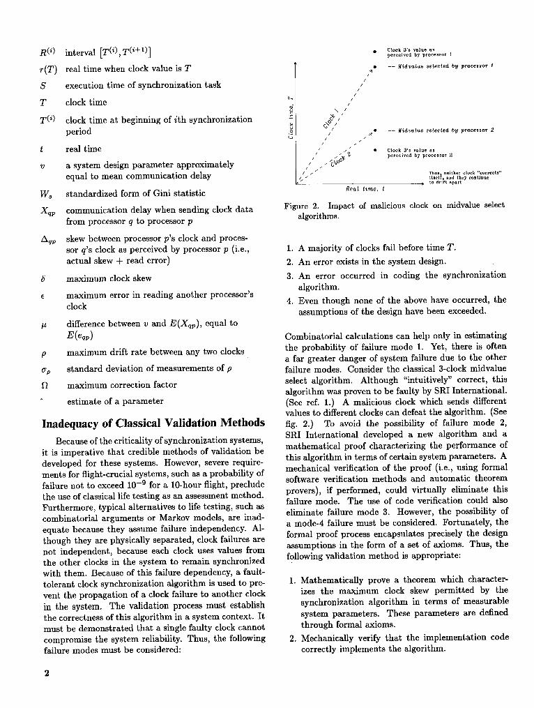
R (_) interval IT (i), T (i+1)] • C,ock3'_,a,...., perceived by processor !

-- fgidvalue selected by processor 1

r(T) real time when clock value is T 4 •/

S execution time of synchronization task/

T clock time _ ,'

T (i) clock time at beginning of ith synchronization = o_ ,• -- Midvalue selecCed by processor 2

period _ ,' _// /

t real time , _ • C_oek3'_,,,....

/ _\0_ _ _ perceived by processor 2v a system design parameter approximately ," __ __/ / _ Thus neither clock "corrects"

equal to mean communication delay _ - .0o,_,.0dt_o_oootl_ot* to drift apart

W_ standardized form of Gini statistic R_t ti_e, t

Xqp communication delay when sending clock data Figure 2. Impact of malicious clock on midvalue selectfrom processor q to processor p algorithms.

Aqp skew between processor p's clock and proces-sor q's clock as perceived by processor p (i.e., 1. A majority of clocks fail before time T.actual skew -4-read error) 2. An error exists in the system design.

5 maximum clock skew 3. An error occurred in coding the synchronizationalgorithm.

E maximum error in reading another processor's4. Even though none of the above have occurred, the

clock assumptions of the design have been exceeded._t difference between v and E(Xqp), equal to

E(%p) Combinatorial calculations can help only in estimating

p maximum drift rate between any two clocks the probability of failure mode 1. Yet, there is oftena far greater danger of system failure due to the other

ap standard deviation of measurements of p failure modes. Consider the classical 3-clock midvalue

12 maximum correction factor select algorithm. Although "intuitively" correct, thisalgorithm was proven to be faulty by SRI International.

estimate of a parameter (See ref. 1.) A malicious clock which sends differentvalues to different clocks can defeat the algorithm. (See

Inadequacyof Classical ValidationMethods fig. 2.) To avoid the possibility of failure mode 2,SRI International developed a new algorithm and a

Because of the criticality of synchronization systems,it is imperative that credible methods of validation be mathematical proof characterizing the performance ofdeveloped for these systems. However, severe require- this algorithm in terms of certain system parameters. Aments for flight-crucial systems, such as a probability of mechanical verification of the proof (i.e., using formalfailure not to exceed 10-9 for a 10-hour flight, preclude software verification methods and automatic theoremthe use of classical life testing as an assessment method, provers), if performed, could virtually eliminate thisfailure mode. The use of code verification could alsoFurthermore, typical alternatives to life testing, such ascombinatorial arguments or Markov models, are inad- eliminate failure mode 3. However, the possibility ofequate because they assume failure independency. A1- a mode-4 failure must be considered. Fortunately, thethough they are physically separated, clock failures are formal proof process encapsulates precisely the designnot independent, because each clock uses values from assumptions in the form of a set of axioms. Thus, thethe other clocks in the system to remain synchronized following validation method is appropriate:with them. Because of this failure dependency, a fault-tolerant clock synchronization algorithm is used to pre- 1. Mathematically prove a theorem which character-vent the propagation of a clock failure to another clock izes the maximum clock skew permitted by thein the system. The validation process must establish synchronization algorithm in terms of measurablethe correctness of this algorithm in a system context. It system parameters. These parameters are definedmust be demonstrated that a single faulty clock cannot through formal axioms.compromise the system reliability. Thus, the following 2. Mechanically verify that the implementation codefailure modes must be considered: correctly implements the algorithm.

2

3. Experimentally verify the axioms required in thedesign proof above. ( 1 + p//2) T

Although the SIFT synchronization code has not yet r (-[)

been mechanically checked, a mathematical design _ _(1-pl//

proof has been performed on the algorithm. Themechanical proof will be performed by SRI Interna-

tional under NASA contract NAS1-17067 during 1984 2)T

and 1985. In the following section, this algorithm and -_its proof are discussed, a:: " _ Good-clock

regionSRI Clock Synchronization Algorithm, )

To discuss the SRI clock synchronization algorithmproperly, it is necessary to introduce a few definitions Clock lime, Tand some notation. The theory in this section was

developed by SRI under the SIFT development contract Figure 3. Definition of a good clock.NAS1-15428 (see ref. 1).

It is convenient to define a clock as a function from T (i) = T (°) + iR, and R (i) = [T(i),T(i+l)]. For eachreal time t to clock time T: C(t) = T. Real time such interval there is a new clock definition as follows:is distinguished from clock time by the use of small

letters for the former and capital letters for the latter. C(i+l)(t) --C(i)(t). A (i)It is sometimes useful to use the inverse clock function

r(T) -- C-I(T) -- t. Using this inverse function, the where A (i) is the ith clock correction.concept of synchronization can be defined as follows: The clock synchronization algorithm requires that

each processor exchange clock values with every otherDefinition: Two clocks rp and rq are synchronized to processor during the subintervalwithin 5 of each other at time T if

S (') = [T ('+1) - S, T(_+I)]Irp(T) - rq(T)l < 5

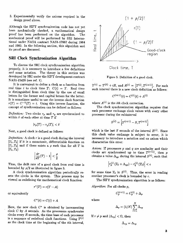
Next, a good clock is defined as follows: which is the last S seconds of the interval R(i). Sincethis clock value exchange is subject to error, it is

Definition: A clock r is a good clock during the interval necessary to introduce a notation and an axiom whichiT1, T2] if it is a monotonic, differentiable function on characterize this error:[211,T21 and if there exists a p such that for all T iniT1, T2]: Axiom: If processors p and q are nonfaulty and their

clocks are synchronized up to time T(i+l), then p

rd_T(T) _ 1 < -p obtains a value Aqp during the interval S(i), such that2

Thus, the drift rate of a good clock from real time is r(i) (To + Aqp) - r_i) (To) < €bounded.by p/2 as illustrated in figure 3.

A clock synchronization algorithm periodically re- for some time To in S (i). Thus, the error in readingsets the clocks in the system. This process may be another processor's clock is bounded by €.viewed as redefining the mathematical clock function: The SIFT synchronization algorithm is as follows:

r*(T) = r(T - A) Algorithm: For all clocks p,

or equivalently C (i+D = C (i) + Ap

C* (t) = C(t) + A whereN

Here, the new clock C* is obtained by incrementing Ap = (l/N)E/_rpclock C by A seconds. As the processors synchronize r=l

clocks every R seconds, the time base of each processor If r _ p and IArpl < 12, thenis a sequence of redefined clock functions. Using T(i)

as the clock time at the beginning of the ith interval, /_rp = Arp

3

else be established by experimentation. The following is a

/_rp _-- 0 list of the system behavior axioms which are assumedin the SRI design proof:

where

_2_-._i . _ 1. The maximum drift rate between any two working

The following theore.m was proved by Leslie Lam- clocks is < p.port and Michael Melliar-Smith of SRI International: 2. If two processors are nonfaulty, then one processor

can read another processor's clock to within an errorTheorem: If of €.

3m < N, 3. The clocks of the system are initially synchronizedto within _io.

_ > N { 2E. p [R . 2 ( NNm ) S] } , 4. ThesystemexecutesthealgorithmeveryRseconds- N - 3m and provides enough CPU time for the algorithm to> _o + pR, complete.

_<<R,Each of these assumptions must be established to a

and confidence level consistent with the reliability require-

(_<< €/p merits. Thus, although life _testing of the system as a

and if no more than m processes are faulty up to time whole can be avoided, life testing must effectively beperformed on certain system parameters. However, the

T (i+1), then for all clocks p and q: behavior of these low-level components of the system

1. If processes p and q are nonfaulty up to time T (i+1), are typically far less complex than the system as athen for all values of T in R (1): whole, and the components are thus easier to validate.

Furthermore, the formal proof provides a precise state-r(i)(T) - r(i)(T) < 5 merit of exactly which properties of the system must be

measured.2. If process p is nonfaulty up to time T (i+1), then

r (i+1) (T) - r (i) (T) < l] Measurement of System ParametersThe mathematical theorem defines the worst-case

where clock skew in terms of certain system parameters. TheseE maximum error in reading another processor's parameters are specific to each implementation of the

clock algorithm. The SIFT system was originally imple-

p maximum drift rate between any two clocks merited on seven Bendix BDX-930 processors. How-ever, extracting synchronization data from that system

m maximum mimber of faulty clocks accommo- is currently difficult. To investigate methods of vali-dated dation, the SIFT synchronization algorithm was imple-

N number of clocks in system mented on four VAX-ll/750 computers in AIRLAB.Some of the system parameters are directly measurable

R synchronization period on the VAX system. Others, such as the maximumS execution time of synchronization task read error _ must be indirectly measured. The results

of these measurements are analyzed in a subsequent sec-Aqp skew between processor p's clock and proces- tion, after the explanation of the theoretical method.

sor q's clock as perceived by processor p (i.e., The first parameter to be discussed is E, because it isactual skew -}- read error) the most difficult to measure and plays a significant role

Assumptions of Design Proof in the system performance. As defined previously, E isan upper bound on [eqpI over all processor pairs and over

The design proof effectively establishes the correct- all time, where eqp -- r (i) (To . Aqp) -- r(i) (To). Unfor-hess of the algorithm, assuming a set of axioms is cor- tunately, Capis defined in terms of real time rather thanrect. Many of these axioms are well-established mathe- observable clock time. In the appendix, the following

matical theorems. Other axioms define the behavior of formula defining Cap in terms of observable clock timesthe computer system on which the algorithm executes, is shown to be a highly accurate approximation of the

For example, the SRI design proof assumes that every theoretical eqp:processor can read another processor's clock to withinan error of _. The correctness of such assumptions must Aqp . eqp : Aqp

and Read clock

leqp[<E IQ(tl))Processor q

where Aqp is the difference between clocks p and q at s_d_-_real time t (i.e., actual skew at t):

I _ Read clock

Aqp(t) = Cp(t) - Cq(t)Processor p . ,_ _,

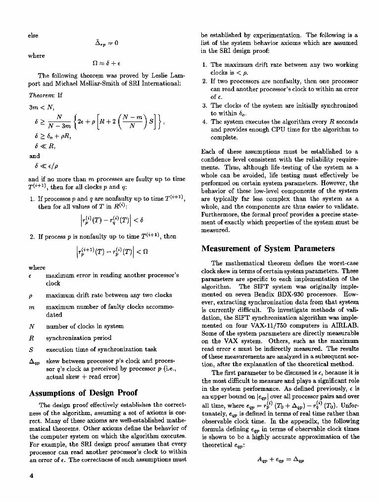
It is still necessary to characterize eqp in a system , R_i,_context. In the system, a processor p reads a processor '4 _

q's clock by the following method: At a prespecified t_ t2time, processor q reads its clock and transmits the value

Cq(Q) to processor p. Upon receiving the message,

processor p immediately reads its clock to obtain Cp(t2). Xqp=cp(t2) - cp(tl)As shown in figure 4, if the exact communication delay Aqp=c/tfl - Cq(_l)=cp_2) - cq_1) - xq_Xap were known, then the exact skew Aqp could be

calculated by Figure 4. Calculation of actual skew Aqp.

Aqp = Cp(t2) - Cq(tl) - Xqpcommunication delay plus the pulse delay were mea-

Thus, the designer of the synchronization system sured. Subtracting an estimate of the mean pulse delaychooses a value v approximately equal to E(Xqp) to from this value provides an accurate measurement of

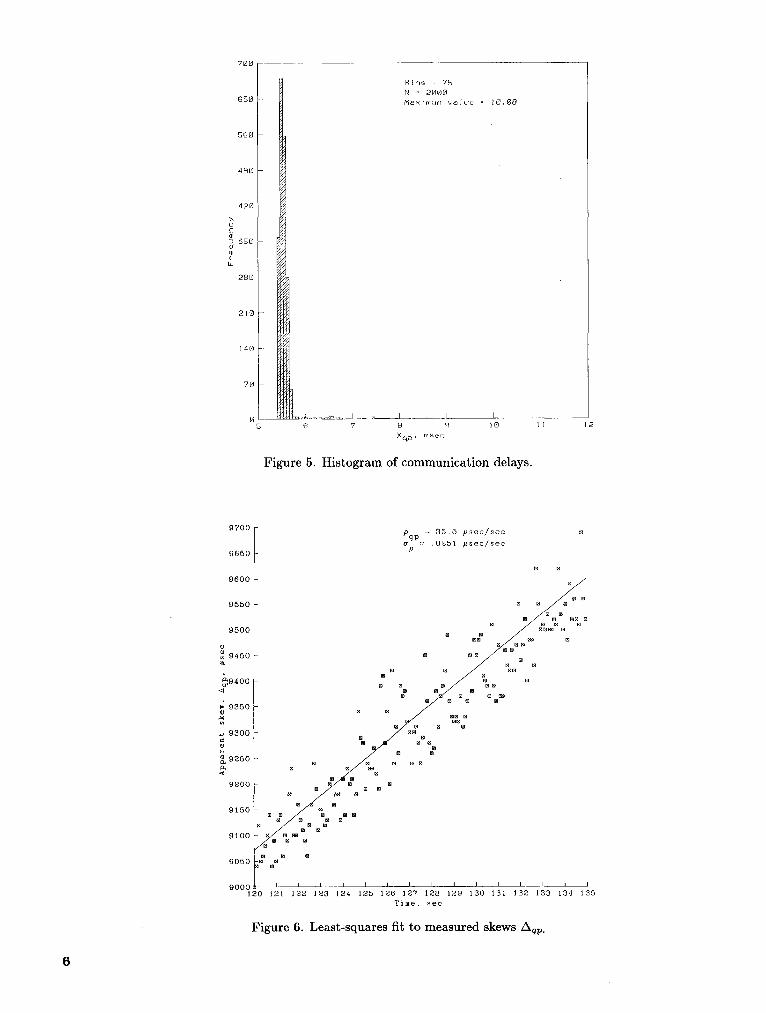
be used by the system to compute an apparent skew the communication delay. Figure 5 is a histogram ofAqp by the following formula: 2000 such estimates of Xqp.

Next, a method is discussed that provides a means ofAqp = Cp(t2) - Cq(tl) - v estimating both Eand p using the internal state informa-

tion of the synchronization system. Thus, the methodBecause the communication delay is variable, each cal-

culation of Aqp is subject to an error of Xqp - v. There requires no special external measuring hardware. Theare two components to this error, and they are shown physics of crystal clocks dictates that the drift rate pqpin the following equation: between any two clocks q and p is constant over time.

Thus, if the system is run without synchronization, the

eqp = Xqp - v = [Xqp - E (Xqp)] +/_ model

where Aqp(T) = 6qp(0) + pqpT + eqp(T)

I_ = S(Xqp)- v describes the system, where 6qp(O) is the initial skewbetween clocks q and p at time 0, and pqp is the drift

The first component [Xqp - E(Xqp)] is the variation rate between clocks q and p. The values of Aqp(T) aredue to the random nature of the communication. The directly observable from the various processors memo-second component _ is a constant offset due to the ries. Since the Aqp's are computed every R seconds,

system designer's error in choosing v. Also, it follows the data consist of Aqp(T(i)), where T(i) = T(0) + iRfrom the above formula that E(eqp) = _. and i = 1, n. Thus, a linear least-squares analysis can

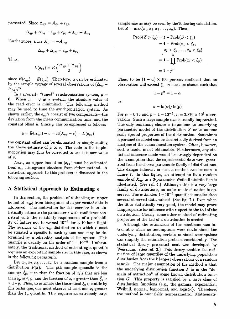
The distribution of eqp may be obtained from mea- be used to estimate the parameters 6qp(0) and pqp. (Seesurements of the one-way communication delays. How- fig. 6.) The residuals from the regression can be repre-ever, this requires some form of special hardware. In sented by €, and the equation can be written as:the AIRLAB VAX system, a special Pulse Network was

used to measure this delay. The delay for sending a Aqp(T) = & +/_T + €pulse is considerably less variable than the communica-

tion delay for sending a message. Thus, reasonably ac- If the eqp'S are distributed with mean zero, then f_curate measurements of the communication delay were is an estimate of PqT, and the residuals have approxi-made by the following method: One processor's clock mately the same distribution as the eqp'S. However, thiswas read, and the value was sent to a second proces- may not be the case. Suppose that E(eqp) = _ _ O.sor. When the second processor received the message, Then, a = 6qp(0) + _u, and the residuals have approxi-a pulse was immediately sent over the Pulse Network mately the same distribution as eqp - _. Thus, a his-to the first processor. When the first processor received togram of eqp's can be obtained by adding _ to thethe pulse, its clock was read again. By subtracting residuals.

the first clock value from the second clock value, the Next, a simple independent method to estimate _ is

7_

Bins _ 7S

N = 2000

650 H_ximum value - I_,08

$60

49_3

42"D

K¢b 5S00_

28D

219 1

140 tL

7_

_,_L.,_x_._L [ ! I. I6 ? 8 9 !13 11 12

Xqp, msec

Figure 5. Histogram of communication delays.

9700= 35.5 #sec/sec

Pqp=

ap .0251 #sec/sec9650

96009550 _ []

9500 _ [] [] _m _[] []

o

e_ 9450 [] o _ _ []

_9400 _ _e [] _ a % _ []

_ 9850

9aoo

_ 9260 ® e _ mD e _ e e

9200 [] _ _ [] _

9150 _ _ _ _ _ []

9100 _ _ m

9050 _ _ ®

9000 I I I I I I I I I I I I I I I120 121 122 123 124 125 126 127 128 129 130 131 132 133 134 135

Time, see

Figure 6. Least-squares fit to measured skews Z_qp.

6

presented. Since Aqp = Aqp -b eqp, sample size as may be seen by the'following calculation.

Let Z = max(x1, x2, x3,..., xn). Then,/kqp --{-Apq = eqp --{-epq -_- Aqp + Apq

Prob(Z > _p) = 1 - Prob(Z < _p)

Furthermore, since Aqp = -Apq, = 1 -Prob(Xl < _p,

Aqp + Apq = eqp + epq x2 < _p, . . . , xn < _p)

Thus, = 1 - H Prob(xi < _v)

E(eqp) = E ( Aqp + Apq ) i2 = 1-p n

since E(eqp) = E(epq). Therefore, /_ can be estimated Thus, to be (1 - _) × 100 percent confident that anby the sample average of several observations of (Aqp + observation will exceed _p, n must be chosen such thatApq)/2.

1-pn = l-olIn a properly "tuned" synchronization system, /_ --0. When /_ -- 0 in a system, the absolute value of orthe read error is minimized. The following methodmay be used to tune the synchronization system. As n--ln(a)/ln(p)

shown earlier, the eqp'S consist of two components--the For a = 0.75 and p = 1 - 10-9, n = 2.876 × l0 s obser-deviation from the mean communication time, and the vations. Such a large sample size is usually impractical.constant offset/z. Since/_ can be expressed as follows: The only remaining choice is to assume an underlying

parametric model of the distribution X or to assume= E(Xqp) - v = E(Xqp - v) = E(eqp) some special properties of the distribution. Sometimes

a parametric model can be theoretically derived from anthe constant offset can be eliminated by simply adding analysis of the communication system. Often, however,the above estimate of/_ to v. The code in the imple- such a model is not obtainable. Furthermore, any sta-mentation may thus be corrected to use this new value tistical inference made would be strongly dependent onof v. the assumption that the experimental data were gener-

Next, an upper bound on [eqp[ must be estimated ated from the chosen parametric family of distributions.from eqp histograms obtained from either method. A The danger inherent in such a method can be seen instatistical approach to this problem is discussed in the figure 7. In this figure, an attempt to fit a random

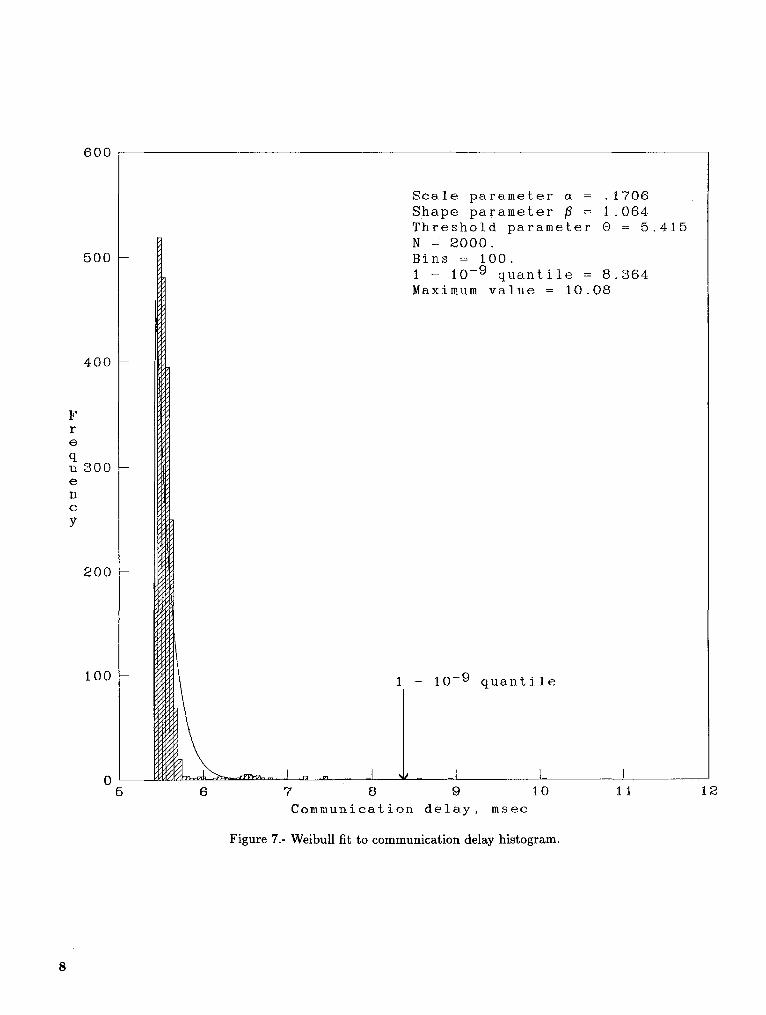
following section, sample of Xqp to a 3-parameter Weibull distribution isillustrated. (See ref. 4.) Although this is a very large

A Statistical Approach to Estimating € family of distributions, an unfortunate situation is ob-served. The estimated 1 - 10-9 quantile is smaller than

In this section, the problem of estimating an upper several observed data values[ (See fig. 7.) Even whenbound of leqpl from histograms of experimental data is the fit is statistically very good, the model may proveaddressed. The motivation for this exercise is to sta- inappropriate for inference with respect to the tail of thetistically estimate the parameter Ewith confidence con- distribution. Clearly, some other method of estimatingsistent with the reliability requirement of a probabil- properties of the tail of a distribution is needed.ity of failure not to exceed 10-9 for a 10-hour flight. Although the estimation of the maximum was in-The quantile of the eqp distribution to which _ must tractable when no assumptions were made about the

be equated is specific to each system and may be de- underlying distribution, certain minimal assumptionstermined by a reliability analysis of the system. This can simplify the estimation problem considerably. Thequantile is usually on the order of 1 - 10-9. Unfortu- statistical theory presented next was developed bynately, the traditional method of estimating a quantile Weissman. (See ref. 2.) This theory enables the esti-requires an exorbitant sample size in this case, as shown mation of large quantiles of the underlying populationin the following paragraph, distribution from the k largest observations of a random

Let xl, x2, x3,..., x,_ be a random sample from a sample. The major assumption of the method is thatdistribution^ F(x). The pth sample quantile is the the underlying distribution function F is in the "do-number _p, such that the fraction of xi's that are less main of attraction" of some known distribution func-

than _p is < p, and the fraction of xi's greater than _p is tion G. This property is satisfied by a large class of_<1-p. Thus, to estimate the theoretical _p quantile by distribution functions (e.g., the gamma, exponential,this technique, one must observe at least one xi greater Weibull, normal, lognormal, and logistic). Therefore,than the _p quantile. This requires an extremely large the method is essentially nonparametric. Mathemati-

7

6OO

Scale parameter a = .1706Shape parameter _ = 1.064Threshold parameter 0 = 5.415N = 2000.

500 - Bins = 100.

1 - 10 -9 quantile = 8.364Maximum value = 10.08

400 -

Fr

e

qn 300 -e

I1o

y

200 -

100 - i - 10 -9 quantile

0 I I I5 6 7 8 9 10 11 3

Communicalion delay, msee

Figure7.- Weibullfittocommunicationdel_ histogram.

8

cally this assumption is as follows: If xl, x2, x3,.. •, xn where

isarandomsamplefromadistributionF(x) andZnis [ki_=lthe l_rgest observed z, then the distribution function an = (Xin)/k -Xknfor Zn is Fn(x). If there exist sequences an > 0 and bnfor all n and a distribution function G such that

andF _(anx+bn)-_a(x) as n-_¢¢

bn = an ln(k) + Xknfor all values of x where G is continuous, then G(x) isan extremal distribution function and F(x) lies in its"domain of attraction." (See ref. 3.) This distribution CASE 2 (G -- PHI):function G must be from one of the following familiesof distributions: 1 - c/n quantile = (k/c)1/azkn

1. LAMBDA(x) = exp(-e -_) (-c_ < x < c_) where2. PHIa(x) = exp(-x -a) (x > 0, a :> 0)

3. PSIa(x) = exp(-(-x) a) (x _ O,a :> O) [ ki_=l ]The theory developed by Weissman makes possible 1/a = ln(Xi,_)/k - ln(Xkn)the estimation of large quantiles of the underlying dis-tribution. His method is based on the result that the k

largest order statistics, when normalized by constants CASE 3 (G = PSI):an and bn, converge in distribution to a k-dimensional

extremal variate (a vector of variables distributed as Since case 3 applies only to negative x, it isthe ordered times at which events occur in a nonhomo- not appropriate for this application and is notgeneous Poisson process). The normalizing constants discussed in detail here.are treated as unknown parameters indexing the lim-iting distribution and are estimated by the method of The remaining problem is the determination of themaximum likelihood. That is, the estimation problem limiting distribution G. It is possible to test the hypoth-

is solved by basing the estimates on the limiting dis- esis that G --- LAMBDA by testing whether the set of

tribution rather than on the underlying distribution of normalized spacings Din, 2D2n,..., (k - 1)D(k-1)n arethe eqp. As indicated subsequently, the quantiles of the independent, identically distributed exponential ran-

underlying distribution may be represented in terms of dom variables, with Din = Zin - Z(i+l)n. Similarly,the parameters an and bn, thereby obtaining maximum the hypothesis G -- PHI can be tested by determin-

likelihood estimates of the quantiles of the underlying ing whether the normalized spacings of In(Xin) are in-distribution, dependent, identically distributed exponential random

For example, by choosing € to be the 1 - 10-9 quan- variables. The Gini statistic can be used for these tests.

tile, the probability of the system exceeding the design (See ref. 4.) The Gini statistic G8 is calculated asassumption is 10-v. The method provides a simple follows:method of calculating the large quantiles, once the lim-

iting distribution family has been determined (i.e., one G8 = lYi - Yj[/2s(s - 1)_of the three listed previously in this section). Fortu- i=1 j=lnately, simple statistical tests are available for making

this determination. These are discussed subsequently, where Yl, Y2,..., Ys is the random sample being testedThe Weissman technique only uses the largest k values for exponentiality. The statistic G8 necessarily liesof the random sample. The choice of the k is arbitrary, between 0 and 1, with values near 0 or 1 indicatingalthough it should be small in comparison with the sam- nonexponentiality. For values of s larger than 20, theple size (e.g., k = 10 and n = 1000). The value of k is standardized form of the Ginl statistic,chosen prior to the examination of the data.

Once-k is chosen and the limiting distribution is de- W_ = [12(s - 1)]1/2(G_ - 0.5)

termined, one of the following calculations is performed _ the Standard Normal, N(0, 1)depending on the limiting distribution. In each case be-

low Xln >_X2n >_ ... >_ Xkn _ ... >_ Xnn represents may be used to determine the significance level. Thus,the order statistics of the random sample, for example, a W8 value of 2.96 indicates an observed

CASE 1 (G -- LAMBDA): significance level of 1 percents and permits the rejectionof the hypothesis that the distribution is exponential

1 - c/n quantile -- an [-ln(c)] + bn with 99-percent confidence.

9

A Statistical Approach to Estimating p The values of ui are easily obtained by using thefollowing formula:

In this section, a method is presented for estimating

p, the maximum drift rate between any two clocks in ui = Pi + t(v, 0)5_the system, such that if pqp represents the drift ratebetween clocks q and p, then where

V =ns --2

PqP < P n8 = number of data points used in regressionanalysis to obtain _ and bifor all clocks q and p. This is precisely design assump-

tion 1 discussed previously. To determine the probabil- 0 = "_i-- (_)ity that this design assumption is violated, it is neces- t(v, 0) = 0 percentage point of student's t distribu-

tion with v degrees of freedomsary to calculate the probability that one or more Pap

exceed the estimated upper bound _, or For n8 > 100, t(v, 0) may be replaced by a percentagepoint of the standard normal distribution. The follow-

Prob(pqp > _) for some q and p ing approximation formula for the normal distribution

F(z) (see ref. 5) is useful for small values of _ (i.e., largeIf there are n processors in the system being vali- z):

dated, then there are nc = (2) drift rates between pro-1 exp(_0.hz2 )

cessor pairs. For simplicity, these are referred to as Pi, 1 - o_= F(z) = 1 zv_where i = 1 to no.

Using the linear regression analysis on the Aap (T (i))

data described previously, a set of estimates Validation of the AIRLAB ExperimentalSystem

{(pi,_2) li= 1, nc}In this section, the methods developed in the pre-

can be obtained, and Pi is an estimate of the drift' rate vious sections are combined into a complete validation

between processor pair i and 5_ is an estimate of the method. This validation method is illustrated by ap-variance of Pi. plication to measurements made on the AIRLAB ex-

From the experimental data, an estimate of the perimental synchronization system. As described previ-upper bound of the drift rates _ must be determined ously, this system consists of four communicating VAX-

such that Prob(max(pi) > _) = _ is sufficiently small. 11/750 computers. These processors exchange clockThe maximum drift rate p may be estimated as values and synchronize themselves usingthe SIFT fault-

follows: tolerant clock synchronization algorithm. As discussedpreviously, the four major design assumptions which

= max(ui) must be validated are as follows:

where ui is defined by: 1. The maximum drift rate between any two workingclocks is < p.

Prob(pi > ui) = "_x/7- a 2. If two processors are nonfaulty then one processorcan read another processor's clock to within an error

The following theorem shows that this estimate is of €.

adequate: 3. The clocks of the system are initially synchronized

Theorem: Prob(max(pi) < _) > 1 - a. to within 50.4. The system executes the algorithm every R seconds

Proof: and provides enough CPU time for the algorithm to

Prob(max(p_) < _) complete.

= Prob(max(pi)< max(ui)) Design assumption 3 corresponds to a process that

= Prob(pl < max(u_),p2 < max(ui),..., would occur at system initialization. Since this pro-cess occurs before system operation, while the aircraft

p,_ < max(ui)) is on the ground, it need not be fault tolerant. If the ini-> Prob(pl < Ul, p2 < u2,..., Pn < Un) tialization process fails, it can be restarted. Detection

,_o of such a failure is not difficult. Design assumption 4 is

= H n_v_-- a intimately connected with the performance character-istics of the test-specimen operating-system scheduler.

-- 1 - _ Analysis of the operating-system scheduler is strongly

10

dependent on the scheduling method employed in the small by improving the measurement technique (i.e.,system. Therefore, it is not possible to present a generic reducing 5p).

method for validation of this assumption. Hence, only A regression analysis of the Aqp(T (i)) experimentalthe first two design assumptions are analyzed in detail, data produced the following table:

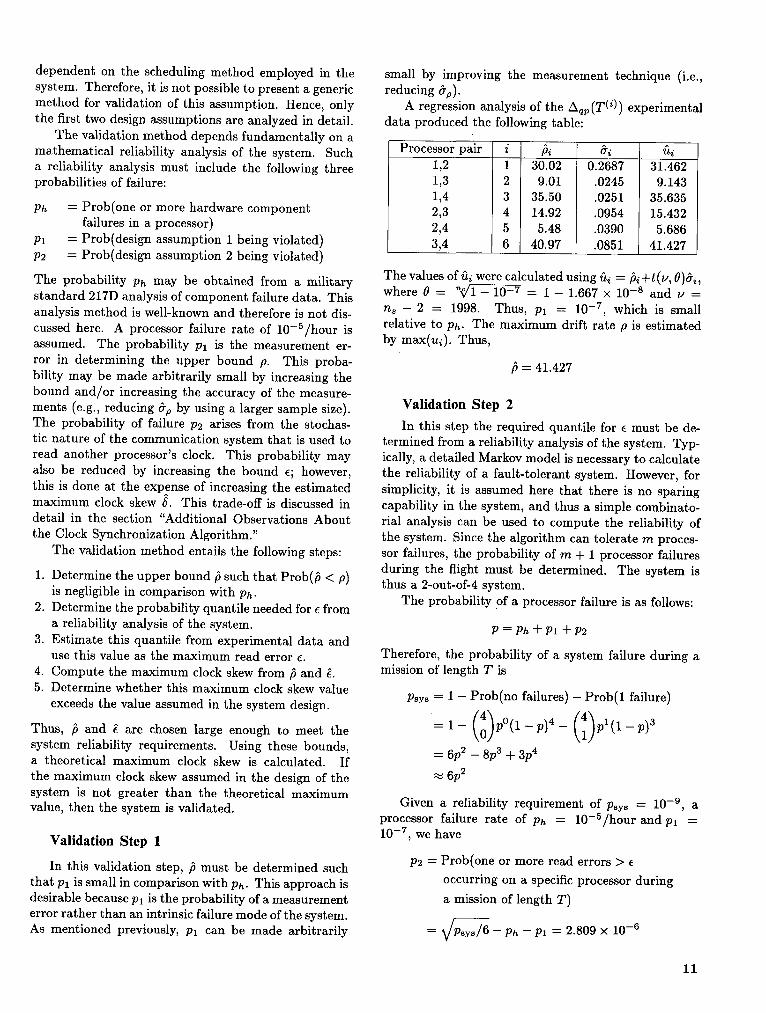
The validation method depends fundamentally on amathematical reliability analysis of the system. Such Processor pair i Pi 5i uia reliability analysis must include the following three 1,2 1 30.02 0.2687 31.462probabilities of failure: 1,3 2 9.01 .0245 9.143

1,4 3 35.50 .0251 35.635Ph ----Prob(one or more hardware component 2,3 4 14.92 .0954 15.432

failures in a processor) 2,4 5 5.48 .0390 5.686Pl -- Prob(design assumption 1 being violated) 3,4 6 40.97 .0851 41.427P2 = Prob(design assumption 2 being violated)

The probability Ph may be obtained from a military The values of ui were calculated using ui = _i+t(u, 0)5_,standard 217D analysis of component failure data. This where _ = "_x/T- 10-7 = 1 - 1.667 × 10-s and _, =analysis method is well-known and therefore is not dis- n8 - 2 = 1998. Thus, Pl = 10-7, which is small

cussed here. A processor failure rate of 10-5/hour is relative to Ph. The maximum drift rate p is estimatedassumed. The probability Pl is the measurement er- by max(ui). Thus,

ror in determining the upper bound p. This proba- _ = 41.427bility may be made arbitrarily small by increasing thebound and/or increasing the accuracy of the measure-

ments (e.g., reducing 5p by using a larger sample size). Validation Step 2The probability of failure P2 arises from the stochas- In this step the required quantile for _ must be de-

tic nature of the communication system that is used to termined from a reliability analysis of the system. Typ-read another processor's clock. This probability may ically, a detailed Markov model is necessary to calculate

also be reduced by increasing the bound €; however, the reliability of a fault-tolerant system. However, forthis is done at the expense of increasing the estimated simplicity, it is assumed here that there is no sparingmaximum clock skew 5. This trade-off is discussed in capability in the system, and thus a simple combinato-

detail in the section "Additional Observations About rial analysis can be used to compute the reliability ofthe Clock Synchronization Algorithm." the system. Since the algorithm can tolerate m proces-

The validation method entails the following steps: sor failures, the probability of m + 1 processor failuresduring the flight must be determined. The system is

1. Determine the upper bound/_ such that Prob(f_ < p) thus a 2-out-of-4 system.is negligible in comparison with Ph. The probability of a processor failure is as follows:2. Determine the probability quantile needed for € from

a reliability analysis of the system. P -- Ph . Pl . P23. Estimate this quantile from experimental data and

use this value as the maximum read error €. Therefore, the probability of a system failure during a

4. Compute the maximum clock skew from f_and _. mission of length T is5. Determine whether this maximum clock skew value

exceeds the value assumed in the system design. Psys -- 1 - Prob(no failures) - Prob(1 failure)/_\ /A\

Thus, _ and _ are chosen large enough to meet the =I-_o)P°(1-p)4-_I)Pl(1-P)3system reliability requirements. Using these bounds,a theoretical maximum clock skew is calculated. If --6p2-8p3. 3p4

the maximum clock skew assumed in the design of the _ 6P2system is not greater than the theoretical maximumvalue, then the system is validated. Given a reliability requirement of Psys = 10-9, a

processor failure rate of Ph = 10-5/hour and pl --

Validation Step 1 10-7, we have

In this validation step, f_ must be determined such P2 -- Prob(one or more read errors > €that Pl is small in comparison with Ph. This approach is occurring on a specific processor during

desirable because Pl is the probability of a measurement a mission of length T)error rather than an intrinsic failure mode of the system.

As mentioned previously, Pl can be made arbitrarily -- _ys/6 - Ph -- Pl ----2.809 × 10 -6

11

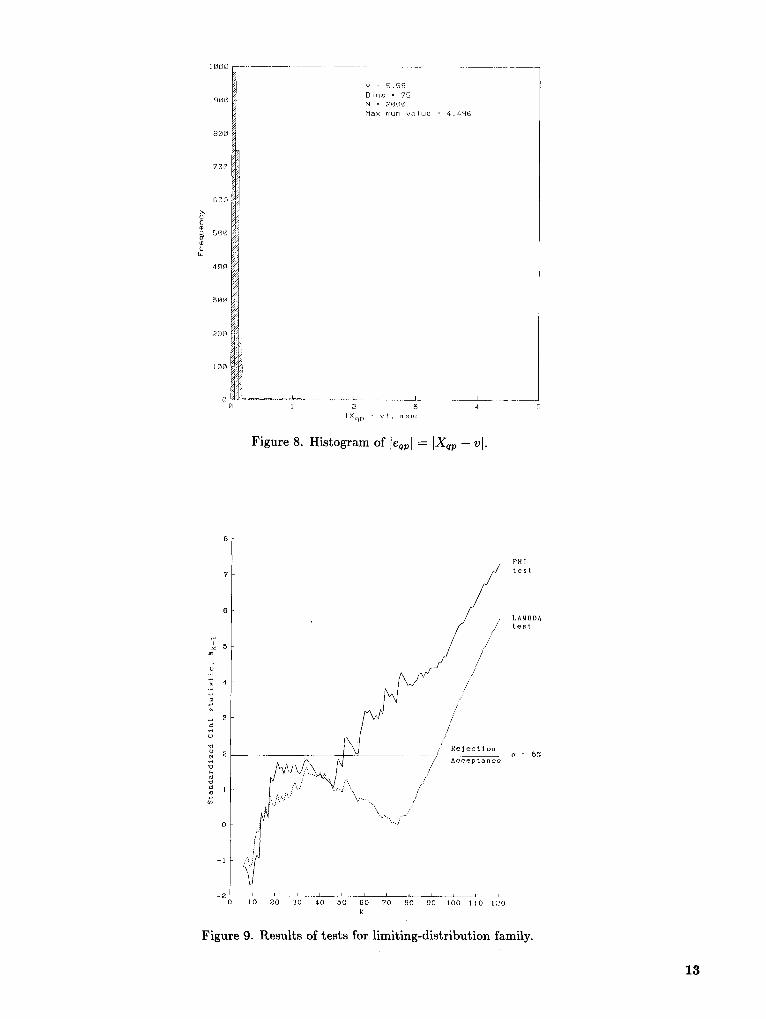
Since the bound _ refers to a single clock read, the examination of the data, k was chosen to be 20 (i.e.,number of clock reads during a mission of length T must 1 percent of the sample), as recommended by Weiss-be determined in order to calculate the quantile needed man. The experimental data best support LAMBDAfor E. as the limiting distribution; however, there was no clear

Defining p_ as rejection of either of the limiting distributions. Thestandardized form of the Gini statistic Wk-1 applied to

p_ = Prob(obtaining a read error > _ the k - 1 normalized spacings of the k largest observa-during a single clock read) tions from the sample, and the corresponding observed

significance levels for the tests were as follows:the probability P2 is then easily expressed in terms ofp_ as follows:

(0) ObservedP2 = 1 - P°( 1 - P_)'_ Limiting significance level,distribution W19 percent

where LAMBDA 0.5262 59.2PHI 1.449 14.7

n = (N - 1)T/R (i.e., the number of clock reads a

specific processor makes during a missionThe inability to choose the limiting distribution with

of length T) precision is of some concern here. Examining theand test results for various values of k provides additional

insight into discerning the limiting-distribution family.T mission time In figure 9, the standardized Gini statistics for the

R synchronization period LAMBDA and PHI tests using various values of kN number of processors in system are plotted. The tests show a consistent tendency

Using the Poisson approximation to the binomial, toward selection of the LAMBDA distribution. In fact,for some values of k there is strong rejection of the

P2 = 1- exp(-np_) PHI and strong acceptance of the LAMBDA. As k

becomes larger, both models are eventually rejected,Furthermore, by a Taylor series approximation (valid because Weissman's theory applies only to the tail ofbecause np_ << 1), a distribution. Although the additional information

obtained by varying k intuitively leads to a choice ofP2 = np_ = (N - 1)(T/R)p_ the LAMBDA distribution, how to use such information

Using N = 4, R = 30 sec, and T = 10 hours, the has not been formalized statistically.

probability p, is determined as follows: An alternate solution to the problem of discerning

p, = 7.805 x 10-l° the limiting-distribution family is to calculate the 1-p_quantile from both family models and to use the most

This analysis assumes independence of clock read- conservative value. However, sometimes the poorly fit-error failures. The design proof has thus reduced the ting model gives astronomical values--leading to unac-strong assumption of independent clock failure to inde- ceptable answers. An alternative approach is to pursue

additional statistical methods to determine the limiting-pendent communication. This analysis makes a strongdistribution family. Such methods are not presentedcase for avoiding contention-based communication pro-

tocols in a fault-tolerant architecture, here.The remaining calculations are performed with the

Validation Step 3 assumption that LAMBDA is the correct limiting dis-tribution. Using the LAMBDA case analysis, the 1-p_

The third step in validating the system under in- quantile was estimated to be 15.383 msec. The combi-

vestigation is to estimate the 1 - p, quantile of the natorial analysis has shown that _ must be at least theread-error distribution. Two methods were developed 1 -p_ quantile to meet the system reliability require-in the preceding sections to obtain a histogram of the

ments. Using this quantile to estimate the upper boundclock read errors eap. Figure 8 is a histogram of

E,leqpl = IXqp - v I obtained from direct measurementsof the one-way communication times. These data are _ = 15.383 msecused to illustrate the determination of _.

As discussed in a preceding section, the upper bound The conservative nature of this estimate can be seen by€ is determined using Weissman's technique. Prior to comparison with the maximum observation, 4.49 msec.

12

]00@ ............

v = 5.G8Bins = 75

qN@N 2_00Maximum value = 4.4£6

800

70_

8@@

5@@

¢C

L

46@

2@@

@ ....... _J_ ...... J L1 2 5 4

IXqp - vl , nlSeC

Figure 8. Histogram of leqpl= IXqp- vl.

8

PHI

7 test

6LAMBDA

/' test

//

//

o /,

_4 ,"

I Rejection_ 2 F a = 5%

._ _ Acceptance

_ /If J "

_ 1 ,:,,,&i",i .,,/"",, /"'\ ,,,v'--,.., ,I"

", ,,,, ,.J

-1

1_ i 210 310 41_ i 61O 710 1_ L a_-2 10 50 80 90 100 llO 120k

Figure 9. Results of tests for limiting-distribution family.

13

Validation Step 4 These validation steps can be reversed to compute

The estimated values of p and E must be inserted system reliability, given a specific design value for theinto the theoretical expression for maximum clock skew maximum clock skew 6. Essentially, p is estimatedfrom the design-proof theorem: as described previously such that pl = 10-7. Then

E is computed from the formula of the theorem using

N { [ ( N ) ]} these values of p and 6. Next, the probability that _ is6 > N - 3------_2€ + p R + 2 N m S , exceeded, P2 can be computed, and hencei Psys can be

6 > 6o + pR, determined. Thus, the system reliability is determined,- given a specific design choice for the maximum clock

5 << R, skew.

andAdditional Observations About the Clock

<< Synchronization Algorithm

The directly measured and indirectly estimated val- The synchronization algorithm is executed periodi-ues of the system parameters are as follows: cally and utilizes CPU time during each execution. The

major component of the execution time is the time re-N = 4 quired to read the clock of every other processor in them = 1 system. In SIFT, each processor's clock value is broad-

R = 30 sec cast during a window of time allocated to it. Thereare N such windows, one for each processor in the sys-

S = 615.334 msec tem. All other processors wait during this window to= 15.383 msec receive the broadcast clock value. To accommodate the

p = 41.42657 ttsec/sec worst-case situation, each window must be at least B+5seconds long, where B is the maximum broadcast time

Using these values, the maximum clock skew 6 can be (i.e., v + €) and 6 is the maximum clock skew. Hence,computed as follows: the execution time for the clock synchronization algo-

5 = [N/(N - 3m)]{2€ + p[R + 2(N - m)S/N]} rithm can be represented as

= 123.061 + 1.65706 × 10-4(30000 + 3(615.334)/2) S = N(5 + B) + K= 123.061 + 5.124

where K is the time needed to compute the correction= 128.185 msec factor and to correct the clock. The execution time of

Thus, the clocks remain synchronized to within the synchronization task S contributes to the inability128.185 msec with probability not less than 1 - 10-9 to synchronize perfectly, because the clocks continue toif the synchronization period is 30 seconds. The contri- drift apart while the synchronization task is executing.bution of the second term is small relative to the first. Thus, the equations defining 6 and S are coupled as

This reveals that, in this implementation, the clocks are follows:much more accurate than the interprocess communica- S = S(N, 5, B, K)tion subsystem. 6 = (N, m, E, p, R, S)

Validation Step 5 Also, € is dependent oir the system reliability require-ment Psys and the synchronization period R. Therefore,

As discussed previously, the communication subsys-

tem of a real-time system depends critically on syn- E---_(psys,R)chronization being maintained within a certain bound.If the calculated skew is less than the bound used in Although an algebraic solution is tedious, 6 can eas-the design of the communication subsystem, then the ily be numerically determined as a function of the syn-synchronization system has been validated. Otherwise, chronization period R or the fraction of time spent syn-

the real-time system must be redesigned if the relia- chronizing S/R. It is more informative, however, tobility requirements are to be met. This may be accom- relate the experimental results to the performance of aplished by either slowing down the communications sys- hypothetical real-time communication system. A real-tem (i.e., waiting longer for interprocess data) or mak- time communication system relies on the synchroniza-ing improvements to reduce p and/or E. The trade-off tion task, as shown in figure 1. The minimum commu-between performance and reliability is explored in detail nication time is B + 6, since the system must wait atin the next section, least this long to insure that the data value has arrived

14

before accessing it. Since B = v + _, the minimum com- explored in detail in this paper. Although the valida-

munication time can be expressed as iv + € + 6). This tion theory is not directly applied to the data obtainedminimum communication time represents the impact of from the SIFT hardware, the validation theory is ap-the synchronization system on the performance of the plied to data obtained from an experimental system inreal-time system. Thus, the performance of the real- the Langley Avionics Integration Research Laboratory

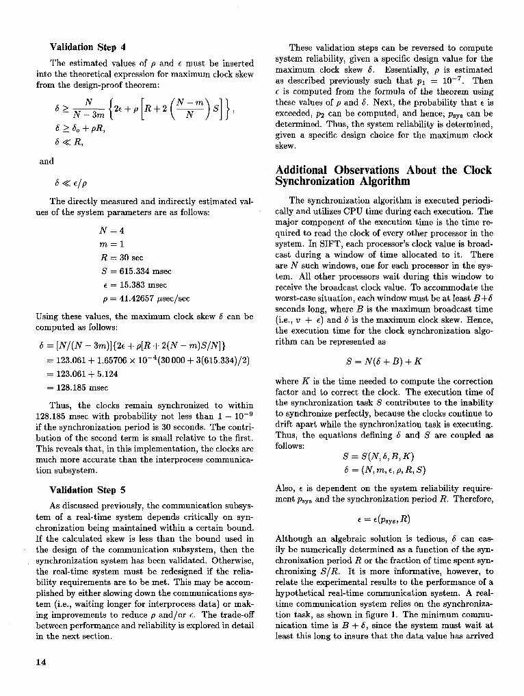
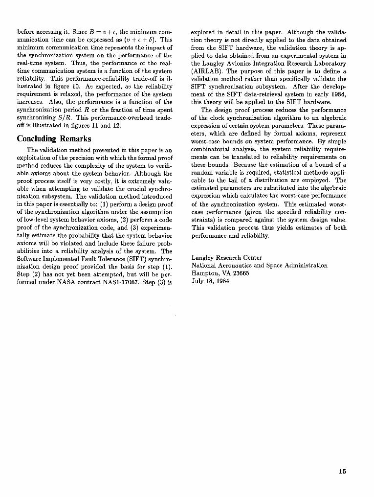
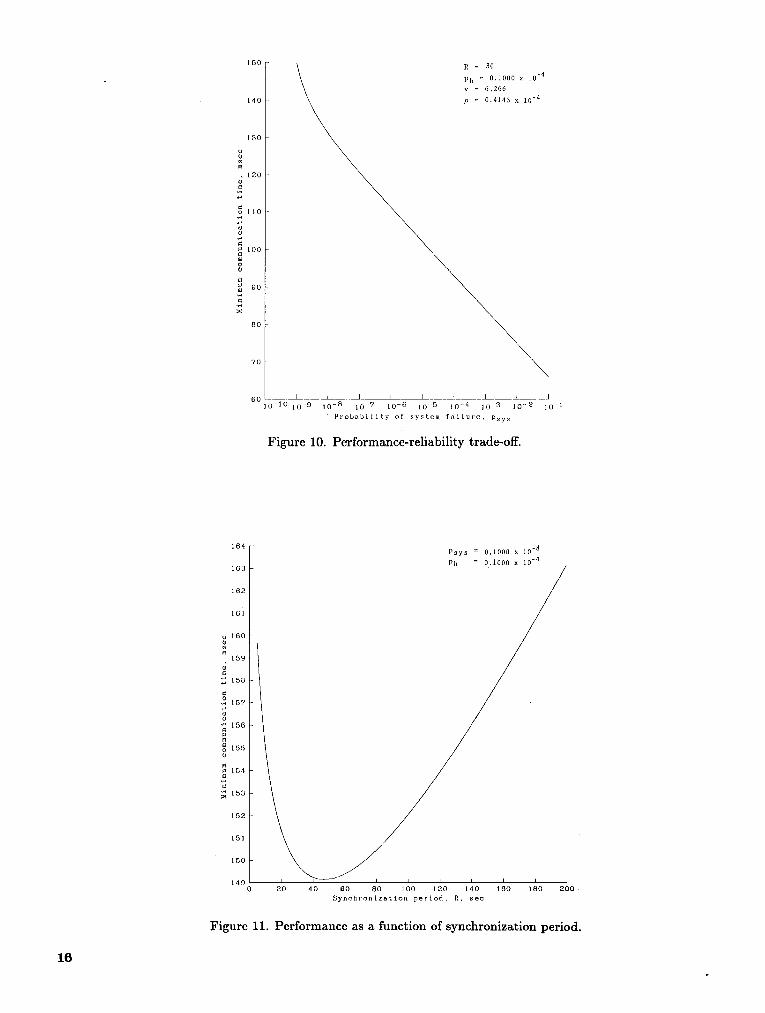
time communication system is a function of the system (AIRLAB). The purpose of this paper is to define areliability. This performance-reliability trade-off is il- validation method rather than specifically validate thelustrated in figure 10. As expected, as the reliability SIFT synchronization subsystem. After the develop-requirement is relaxed, the performance of the system ment of the SIFT data-retrieval system in early 1984,increases. Also, the performance is a function of the this theory will be applied to the SIFT hardware.synchronization period R or the fraction of time spent The design proof process reduces the performancesynchronizing S/R. This performance-overhead trade- of the clock synchronization algorithm to an algebraicoff is illustrated in figures 11 and 12. expression of certain system parameters. These param-

eters, which are defined by formal axioms, representConcluding Remarks worst-case bounds on system performance. By simple

The validation method presented in this paper is an combinatorial analysis, the system reliability require-exploitation of the precision with which the formal proof ments can be translated to reliability requirements onmethod reduces the complexity of the system to verifi- these bounds. Because the estimation of a bound of aable axioms about the system behavior. Although the random variable is required, statistical methods appli-proof process itself is very costly, it is extremely valu- cable to the tail of a distribution are employed. Theable when attempting to validate the crucial synchro- estimated parameters are substituted into the algebraicnization subsystem. The validation method introduced expression which calculates the worst-case performancein this paper is essentially to: (1) perform a design proof of the synchronization system. This estimated worst-of the synchronization algorithm under the assumption case performance (given the specified reliability con-of low-level system behavior axioms, (2) perform a code straints) is compared against the system design value.

proof of the synchronization code, and (3) experimen- This validation process thus yields estimates of bothtally estimate the probability that the system behavior performance and reliability.axioms will be violated and include these failure prob-abilities into a reliability analysis of the system. The

Software Implemented Fault Tolerance (SIFT) synchro- Langley Research Centernization design proof provided the basis for step (1). National Aeronautics and Space AdministrationStep (2) has not yet been attempted, but will be per- Hampton, VA 23665

formed under NASA contract NAS1-17067. Step (3) is July 18, 1984

15

160 R = 30

Ph = 0.1000 x 10 -4

v = 6.266

140 p = 0,4143 x 10 -4

130

• 120

,o

_ 11o

o

100

o

_ 9o

80

7O

60 ______i .... __ .... A_ t I .... _...... L.__.i ......... JlO -10 1o -9 10 -8 10 -7 lO -6 1o -5 10 -4 1o 3 10-2 10-1

Probability of system failure, Psys

Figure 10. Performance-reliability trade-off.

164Psys = 0.1000 x 10 -8

Ph = o. Jo00 X 10 -4160

162

16i

160

159

d158

._ 16"7

'_ 156

155o

154m

153

152

15!

150

I I I I I I1490 20 40 60 80 100 120 140 160 180 200

SynchronizaLlon period, R, sec

Figure 11. Performance as a function of synchronization period.

16

164 - -8Psys = 0.1000 x 10 -4Ph = 0.1000 x 10

163

162

161

o 1600

i59o

"_ i58

0._ i57

0"_ i56

o 1550

154

*r-'l

"_ 153

152

151

150

149 I 1 I I I I I I I tO. .01 .02 .03 .04 .05 .06 .07 .08 .09 .10 .11 .12 .13 .14

Fraction of time synchronizing, S/R

Figurel2. Per_rmance-overheadtrade-off.

17

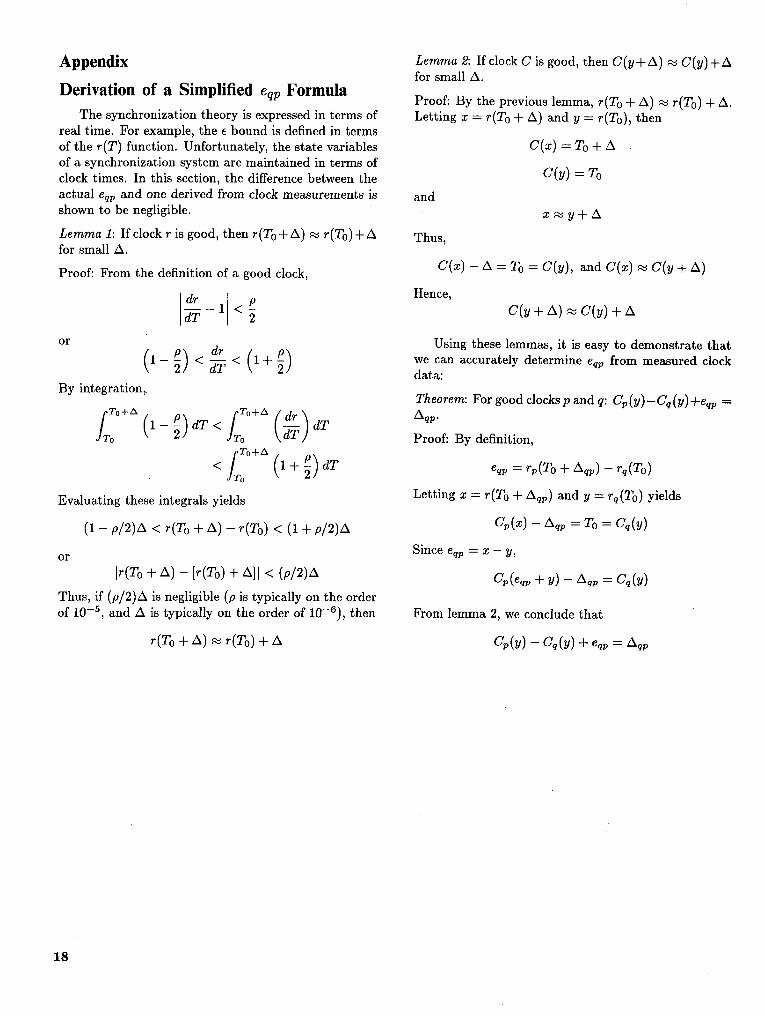
Appendix Lemma 2: If clock C is good, then C(y.A) _ C(y)+Afor small A.

Derivation of a Simplified eqp FormulaProof: By the previous lemma, r(To . A) _ r(To) . A.

The synchronization theory is expressed in terms of Letting x = r(To . A) and y = r(To), thenreal time. For example, the E bound is defined in termsof the r(T) function. Unfortunately, the state variables C(x) = To . Aof a synchronization system are maintained in terms ofclock times. In this section, the difference between the C(y) = To

actual eqp and one derived from clock measurements is and

shown to be negligible, x _ y . A

Lemma 1: If clock r is good, then r(To+A) _ r(To)+A Thus,for small A.

Proof: From the definition of a good clock, C(x) - A -- To = C(y), and C(x) _ C(y + A)

dr p Hence,- 1 < _ c(y + A)_ c(y)+ A

or Using these lemmas, it is easy to demonstrate that

(P)I- _ < _dr(p)< 1 + _ data:Wecan accurately determine eqp from measured clock

By integration, Theorem: For good clocks p and q: Cp(y)-Cq(y).eqp =

fTo+h (l_P) dT< _ dTJ To Proof: By definition,

< 1+ _ aT eq,= rp(To+ Aqp)- r_(To)

Evaluating these integrals yields Letting x = r(To + Aqp) and y = rq(To) yields

(1- p/2)A< r(To+A)- r(To)< (1+ p/2)A C_(x)- Aq,= To= Cq(y)Since eqp = x - y,or

It(To + A) - [r(T0) + All < (p/2)A Op(eq, + y) - Aqp -- Cq(y)

Thus, if (p/2)A is negligible (p is typically on the order

of 10-5, and A is typically on the order of 10-6), then From lemma 2, we conclude that

r(To+ A)_ r(To)+ A Cp(y)- C_(y)+eqp=Aqp

18

References1. Goldberg, Jack; Kautz, William H.; Melliar-Smith, 3. Pickands, James, III: Statistical Inference Using Extreme

P. Michael; Green, Milton W.; Levitt, Karl N.; Schwartz, Order Statistics. Ann. Stat., vol. 3, no. 1, Jan. 1975, pp. 119-Richard L.; and Weinstock, Charles B.: Development andAnal- 131.

ysis of the Software Implemented Fault- Tolerance (SIFT) Computer. 4. Lawless, J. F.: Statistical Models and Methods for Lifetime Data.NASA CR-172146, 1984. John Wiley _z Sons, Inc., c.1982.

2. Weissman, Ishay: Estimation of Parameters and Large Quan- 5. Feller, William: An Introduction to Probability Theory and Its

tiles Based on the k Largest Observations. J. American Star. Applications--Volume I, Third ed. John Wiley & Sons, Inc.,Assoc., vol. 73, no. 364, Dec. 1978, pp. 812-815. 1968, pp. 174-179.

19

1. ReportNo. 2. GovernmentAccessionNo. 3. Recipient'sCatalogNo.NASA TP-2346

-4. Title and Subtitle 5. Report Date

September 1984VALIDATION OF A FAULT-TOLERANT CLOCK SYNCHRONIZATIONSYSTEM 6. PerformingOrganizationCOde

505-34-13-31

7. Author(s) 8. Performing Organization Report No.

Ricky W. Butler and Sally C. Johnson L-15799i0. Work Unit No.

9. Performing Organization Name and Address

NASA Langley Research Center "11.Contractor GrantNo.Hampton, VA 23665

13. Type of Report and Period Covered

12. Sponsoring Agency Name and Address Technical Paper

National Aeronautics and Space Administration '14, Sponsoring AgencyCodeWashington, DC 20546

'15. Supplementary Notes

16. Abstract

This paper presents a new validation method for the synchronization susbystem of a fault-tolerant computer system.The method combines formal design verification with experimental testing. The design proof reduces the correctnessof the clock synchronization system to the correctness of a set of axioms which are experimentally validated. Sincethe reliability requirements are often extreme, requiring the estimation of extremely large quantiles, an asymptoticapproach to estimation in the tail of a distribution is employed.

i .

17. Key-Words (Suggested by Authoris)) 18. Distribution Statement

Validation Unclassified--UnlimitedFault tolerance

Clock synchronizationVerification

Reliability analysis Subject Category 62

19. Security Classif. (of this report) 20. Security Classif. (of this page) 21. No. of Pages 22. Price

Unclassified Unclassified 21 A02

Forsale bythe NationalTechnicalInformationService,Springfield,Virginia 22161 NASA-Langley,]984

National Aeronautics and THIRD-CLASS BULK RATE Postageand Fees PaidNational Aeronautics and

Space Administration Space AdministrationNASA-451

Washington, D.C.20546

Official Business

Penalty for Private Use, $300

N_l_ A POSTMASTER: If Undeliverable (Section 158Postal Manual)Do Not Return