Geophysics 223 January 2009

1

223 B5 Two-dimensional 2-D resistivity model B5.1 Pseudosection display for a Wenner array

• Depth sounding can determine the depth variation of resistivity at a point. • Profiling with an array of fixed a-spacing can determine horizontal variations in

resistivity along a profile.

• To image realistic 2-D resistivity structures, profiling and depth sounding must be combined. This is implemented by using an array of electrodes in a technique that is often call electrical resistivity tomography (ERT)

• The figure on page 2 shows an array of 10 electrodes that is placed in the ground

at the start of the survey. Using an automated cable, each electrode can be activated as a current (red) or potential (green) electrode.

• The first row shows a traverse with a Wenner array that consists of 4 adjacent

electrodes. This is labeled as n=1 spacing to indicate that the array consists of adjacent electrodes. This gives information about resistivity variations close to the surface.

The apparent resistivity value is measured and plotted on the pseudosection with (a) Horizontal position at the centre of the 4-electrode array, (b) Depth that corresponds to the electrode spacing (the large black dot). This is

based on the observation in 223B2 that electric currents go to a depth approximately equal to the a-spacing of the array.

• The second row on page 2 shows a traverse with n = 2, giving information about

resistivity at greater depth. The larger size of the n = 2 array restricts the number of horizontal data points, hence the triangular shape of the pseudosection.

• One reason that the pseudosection is “pseudo”, is that it does not give a true

measure of depth. The depth of exploration increases with n. However there is no simple equation to relate n to the depth of investigation.

• The true depth must be determined by subsequent data analysis.

• However, as we will see below, the pseudosection can give a general impression

of how resistivity varies beneath the electrode array.

Geophysics 223 January 2009

2

Geophysics 223 January 2009

3

B5.2 Wenner pseudosections for 2-D resistivity models

• The following figures were generated using the RES2DMOD software package developed by Dr. M.H. Loke. (http://www.geoelectrical.com/download.html)

• Note that the pseudosection (top) and model (bottom) use different colour scales.

• In these figures pseudo-depth (Psz) is plotted on the vertical axis (not n).

Electrode spacing is L = 1 m and 48 electrodes are used. PsZ = nL/2

• Upper panel shows the pseudo-sections with pseudo depth values on vertical axis. Each point is measured in turn as described on page 2. The apparent resistivity values are then contoured for display.

Example 1

• This model has a 100 Ωm surface layer that overlies a 1 Ωm halfspace. • Lower model has a 3 m thick layer. The lower layer becomes obvious in the

pseudosection at approximately PsZ = 2 m (n = 4)

Geophysics 223 January 2009

4

• In the upper model the surface layer is just 1 m thick, and the lower layer can be detected at PsZ = 1 m (n = 2)

• In this case the pseudosection looks similar to the true resistivity model. This is

not always the case.

• Because the true resistivity of the Earth is 1-D, the apparent resistivity does not vary with horizontal position. Thus the pseudosection is a set of horizontal stripes.

• This is an example of a forward problem in geophysics. A model of the Earth is

used to predict what would be measured in a geophysical survey. Example 2

• This example shows a dipping interface. The upper layer is resistive (100 Ωm) and the lower layer has a lower resistivity (1 Ωm)

• Apparent resistivity decreases as PsZ increases.

• On the left side of the model, apparent resistivity decreases at PsZ = 1m

• On the right side of the model the low resistivity layer is deeper and a PsZ value

of 2 is needed to “see” the low resistivity layer.

• Again, the pseudosection gives a good impression of the true resistivity.

Geophysics 223 January 2009

5

Example 3

• This model shows a 3-layer resistivity model. • The predicted apparent resistivity values in the pseudo-section could be verified

using the MATLAB code described in B3.

• Apparent resistivity in the pseudosection decreases from PsZ = 0.5 to 2 m as the second layer is sampled by the electric currents (n = 1 to 4)

• Apparent resistivity in the pseudosection increases from PsZ = 2-8 m as the third

layer is sampled (n = 4 to 16)

• The array is not large enough to sample the true resistivity of the lowest layer (1000 Ωm)

Geophysics 223 January 2009

6

Example 4

• A conductive 1 Ωm prism is embedded in a 100 Ωm halfspace. • The pseudosection correctly identifies the location of the top of the conductor.

• The pseudosection also shows the correct horizontal extent of the prism.

• Note that the shape is distorted with a wedge shaped region of low resistivity on

each side of the prism.

• This illustrates another aspect of pseudosections which is the fact that the shape can be distorted.

Geophysics 223 January 2009

7

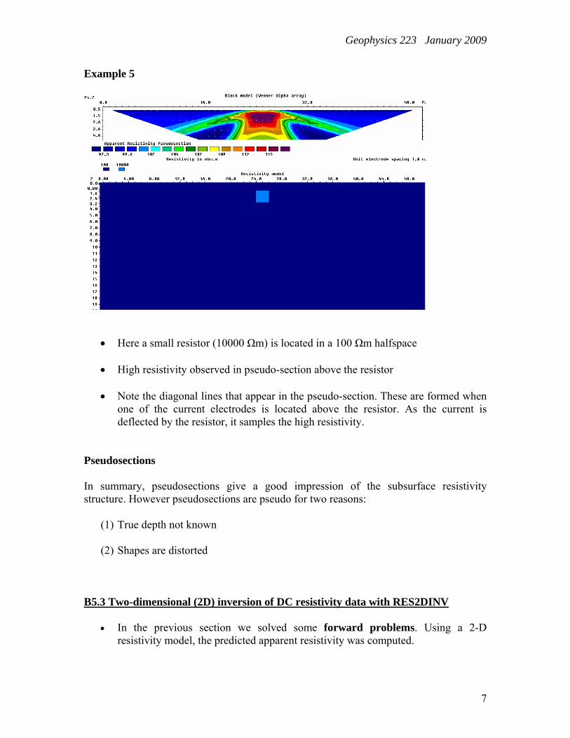
Example 5

• Here a small resistor (10000 Ωm) is located in a 100 Ωm halfspace • High resistivity observed in pseudo-section above the resistor

• Note the diagonal lines that appear in the pseudo-section. These are formed when

one of the current electrodes is located above the resistor. As the current is deflected by the resistor, it samples the high resistivity.

Pseudosections In summary, pseudosections give a good impression of the subsurface resistivity structure. However pseudosections are pseudo for two reasons:

(1) True depth not known (2) Shapes are distorted

B5.3 Two-dimensional (2D) inversion of DC resistivity data with RES2DINV

• In the previous section we solved some forward problems. Using a 2-D resistivity model, the predicted apparent resistivity was computed.

Geophysics 223 January 2009

8

• Most often in exploration geophysics we wish to go in the opposite direction. Data is collected in a survey and we would like to know what resistivity model is present. This is the inverse problem.

• The inverse problem can be solved using a trial-and-error approach. The model is

systematically changed until the predicted data gives a good match to the measured survey. This was the approach we used for 1-D Wenner array data in 223B3. It works in 2-D but can be tedious as there are many parameters to be varied.

• A quicker (and more popular approach) is to solve the inverse problem with an

automated inversion program. RES2DINV is a widely used software package.

B5.3.1 Synthetic 2-D inversions with RES2DINV • When using an inversion program such as RES2DINV, it is very useful to do

some synthetic inversions before inverting real field data. Synthetic inversions use data that was computed for a known resistivity model. This allows the final model to be compared with the true model.

Synthetic inversion - Example 5 from B5.2

• Upper panel shows the “measured data” obtained from RES2DMOD in B5.2.

• The inversion computes a resistivity model (lower panel) and shows the data

calculated (predicted) for this resistivity model (middle panel).

• If the “measured data” and “calculated data” agree well, the inversion stops.

Geophysics 223 January 2009

9

• If the agreement is not adequate, another iteration is performed and the measured data and predicted data are compared (and so on).

• The free version of RES2DINV only does 3 iterations. This is not usually

enough, and it is a good idea to buy a license to permit 10-20 iterations.

• Inversion must account for the fact that the inverse problem is non-unique. This means that many models can be found that fit the measured data. To overcome this problem, a common approach is to choose the smoothest model. This

Synthetic inversion example from Loke (2000)

• The following examples of using RES2DINV are taken from Loke (2000) • The black lines in (b) and (c) show the features present in the resistivity model

used to generate the “measured data”.

Geophysics 223 January 2009

10

B5.3.2 Examples of RES2DINV applied to real data Example from agriculture (Denmark)

Example from mineral exploration showing a dike (Sweden)

Geophysics 223 January 2009

11

B5.4 Pseudosection for a dipole-dipole array

• An alternative electrode configuration can used in array studies as shown below. It can be shown that this can be more sensitive to certain geometries in the subsurface. However, large currents are needed to make reliable measurements, since most current is localized between the two current electrodes (red).

• The dipole-dipole method can also be used for deep DC resistivity exploration.

This is because cables are not needed to connect the current electrodes (a transmitter) and the potential electrodes (a receiver). However, a large power source such as a generator is needed to get data with offsets of several kilometers.

Geophysics 223 January 2009

12

References

M.H. Loke, Electrical imaging surveys for environmental and engineering studies: A practical

guide to 2-D and 3-D surveys, 2000. This can be downloaded at: www.geoelectrical.com in the section “Free software and notes”.