22 Use of mathematical modelling to study biofilm

[ 1 ]

22

Use of mathematical modelling to study biofilm development and morphology

C. Picioreanu and M.C.M. van Loosdrecht

22.1 MATHEMATICAL MODELLING AND BIOFILMS

22.1.1 Why make mathematical models Although the word "modelling" is used for different purposes, the final result is invariably the same: models are no more than a simplified representation of reality based on hypotheses and equations used to rationalize observations. By providing a rational environment, models can lead to deeper and more general understanding. Ultimately, understanding the underlying principles becomes refined to such a state that it is possible to make accurate predictions.

In general, a quantitative representation of the studied system is superior to a merely qualitative picture. What better way is then to describe quantitatively any

2 Biofilms in Medicine, Industry and Environmental Biotechnology

system than by encoding the information in sets of numerical relations? This is exactly the goal of hypotheses expressed in mathematical form, called mathematical models. Mathematical models consist of sets of equations containing in an abstract body the information needed to simulate a system.

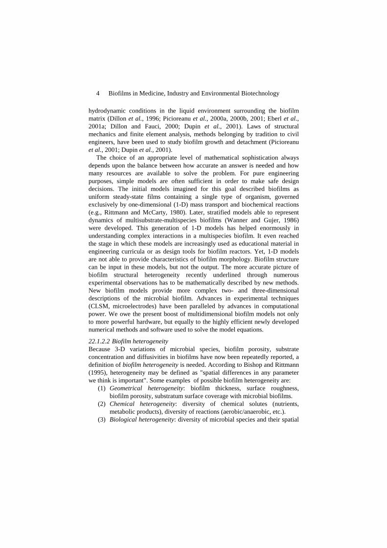
Bailey (1998) gave reasons for justifying the use of modelling in biochemical engineering. These reasons are rephrased below in terms of biofilm modelling: (1). To organize disparate information into a coherent whole. Plenty of data on biofilm structure are now available from computerized experimental techniques. The general view on biofilm structure was dramatically changed by the use of Confocal Scanning Laser Microscopy (CSLM) and computerised image analysis tools, which revealed a more complex picture of biofilm morphology (Lawrence et al., 1991; Caldwell et al., 1993, Costerton et al., 1994). Cell clusters may be separated by interstitial voids and channels, which create a characteristic porous structure. In some particular cases, biofilms grow in the form of microbial clusters taking a "mushroom" shape. However, biofilms may be regularly with homogeneous compact layers of microorganisms in a slime matrix. Mathematical models can answer what all these structures have in common and what leads to differences. It cannot be anymore a reason in itself acquiring impressive 3-D images of biofilm structure. Constructing a mathematical model that explains the formation of biofilm morphology should complement interpretation of 3-D images of biofilm structure. (2). To think about and calculate logically what components and interactions are important in a complex system. It is a common situation to have sets of experimental data from different laboratories, which lead to often opposing qualitative interpretations. When hypotheses can be expressed as mathematical models, the task of testing the theories becomes easier because experimental data from various sources can be directly and quantitatively compared. For example, formation of finger-like biofilms has been attributed to the control of the genome of microorganisms involved (e.g., Davies et al., 1998). The hypothesis of cell-to-cell signalling was initially suggested as a result of the difficulty in explaining by other physical mechanisms the pore formation in biofilms. However, using only laws of physics that are generally valid, regardless of the particular biological system studied, the formation of a variety of heterogeneous biofilm structures can be logically explained (Picioreanu et al., 1998b; Picioreanu, 1999). (3). To make important corrections in the conventional wisdom. An illustrative example is the belief that convective transport of nutrients through biofilm channels significantly contributes to the increased mass transfer from bulk liquid into the biofilm. Numerical simulations of flow and mass transfer with the 2-D and 3-D biofilm models by Picioreanu et al. (2001) and Eberl et al. (2001a) clearly show that for the usual hydrodynamic regimes, diffusion and not

Mathematical Modelling of Biofilm Morphology 3

convection is the dominating mass transport mechanism in biofilms. Although there is flow inside the channels, the flux of nutrient transported is minimum, and the channels cannot be seen as nutrient suppliers to deep layers of bacteria. (4). To understand the essential qualitative features of a complex system. Again, the example of finger-like biofilms is suggestive. As the following sections of this review will make clear only three processes - diffusion, reaction and microbial growth - are essential to explain, at least qualitatively, formation of heterogeneous biofilms. (5). To discover new strategies. Different types of biofilm structure are needed for different engineering applications like wastewater treatment. Whereas smooth and compact biofilms are desired for settleability in particle biofilm reactors, fluffy biofilms can be advantageous in bio-filtration units by better catching the solid impurities. Engineering biofilm structure based on model predictions could eventually lead to the formation of the desired biofilm type in a particular reactor system.

22.1.2 How to make mathematical models 22.1.2.1 Models based on first-principles Mathematical models can be derived in two ways, somehow opposing, but nevertheless complementary. The first approach, which is often the expedient choice, is to build empirical relationships from analysis of observations. These black-box correlations are strictly restricted to the conditions in which the experimental data were obtained, and extrapolation is hazardous. The second line, which we shall approach in this review, is to represent reality based on fundamental laws of physics, chemistry and biology. These general laws are also called first principles. The development of models based on first principles of science leads invariably to strengthening the intuitive process and to developing orderly and rational methods for approaching a problem. As an example, biofilm models based on reaction/transport principles (e.g., Wanner and Gujer, 1986) have proved useful not only to test soundness of different scientific concepts, but also to establish rational strategies for many design problems involving biofilms. Models based on first principles promote lateral transfer of insight between various scientific domains. Diffusion/reaction models routinely used in chemical engineering are now widely used to simulate biofilm systems (Wanner and Gujer, 1986; Wanner and Reichert, 1996). Stochastic models for crystal growth based on diffusion-limited aggregation can also explain formation of bacterial colonies (e.g., Matsushita and Fujikawa, 1990; Ben-Jacob et al. 1994). Fluid mechanics methods have been applied to study biofilm rheology (Dockery and Klapper, 2001; Stoodley et al., 1999) and


hydrodynamic conditions in the liquid environment surrounding the biofilm matrix (Dillon et al., 1996; Picioreanu et al., 2000a, 2000b, 2001; Eberl et al., 2001a; Dillon and Fauci, 2000; Dupin et al., 2001). Laws of structural mechanics and finite element analysis, methods belonging by tradition to civil engineers, have been used to study biofilm growth and detachment (Picioreanu et al., 2001; Dupin et al., 2001).

The choice of an appropriate level of mathematical sophistication always depends upon the balance between how accurate an answer is needed and how many resources are available to solve the problem. For pure engineering purposes, simple models are often sufficient in order to make safe design decisions. The initial models imagined for this goal described biofilms as uniform steady-state films containing a single type of organism, governed exclusively by one-dimensional (1-D) mass transport and biochemical reactions (e.g., Rittmann and McCarty, 1980). Later, stratified models able to represent dynamics of multisubstrate-multispecies biofilms (Wanner and Gujer, 1986) were developed. This generation of 1-D models has helped enormously in understanding complex interactions in a multispecies biofilm. It even reached the stage in which these models are increasingly used as educational material in engineering curricula or as design tools for biofilm reactors. Yet, 1-D models are not able to provide characteristics of biofilm morphology. Biofilm structure can be input in these models, but not the output. The more accurate picture of biofilm structural heterogeneity recently underlined through numerous experimental observations has to be mathematically described by new methods. New biofilm models provide more complex two- and three-dimensional descriptions of the microbial biofilm. Advances in experimental techniques (CLSM, microelectrodes) have been paralleled by advances in computational power. We owe the present boost of multidimensional biofilm models not only to more powerful hardware, but equally to the highly efficient newly developed numerical methods and software used to solve the model equations.

22.1.2.2 Biofilm heterogeneity Because 3-D variations of microbial species, biofilm porosity, substrate concentration and diffusivities in biofilms have now been repeatedly reported, a definition of biofilm heterogeneity is needed. According to Bishop and Rittmann (1995), heterogeneity may be defined as "spatial differences in any parameter we think is important". Some examples of possible biofilm heterogeneity are:

(1) Geometrical heterogeneity: biofilm thickness, surface roughness, biofilm porosity, substratum surface coverage with microbial biofilms.

(2) Chemical heterogeneity: diversity of chemical solutes (nutrients, metabolic products), diversity of reactions (aerobic/anaerobic, etc.).

(3) Biological heterogeneity: diversity of microbial species and their spatial


distribution, differences in activity (growing, EPS producing, dead cells) (4) Physical heterogeneity: biofilm density, permeability, visco-elasticity,

mechanical strength, solute diffusivity, presence of abiotic solids, etc. It can be stated that geometrical heterogeneity causes in a great measure the

other kinds of heterogeneity. A proper description of biofilm geometrical morphology is probably the basis for a good description of the other types of heterogeneity. Biofilms are multiphase systems, comprising solid particles, a liquid phase and, in some cases, a gas phase. From the modelling point of view, we understand the “biofilm” as being only the solid phase, which includes the extracellular polymeric gel, microbial cells and other entrapped particles of biotic or abiotic origin. The geometrical structure of a biofilm is the spatial arrangement of particulate biofilm components. Therefore, the dynamics of solid matter (gel, cells, other solids) produces the biofilm geometrical heterogeneity.

22.1.2.3 Essential processes in biofilm models During biofilm development, a large number of phenomena occur over a wide range of length and time scales. It is necessary first to assemble knowledge about the various processes occurring in the biofilm system. Modelling the structural development of a biofilm is challenging just because of this complex interaction between many processes. The biofilm development is determined on one hand by “positive” or “gain” processes, like cell attachment, cell growth and division, and polymer production, which lead to biofilm volume expansion. On the other hand, “negative” or “loss” processes, like cell detachment and cell death, may contribute to biofilm shrinking. By changing the balance between these two types of processes, biofilms with different structural properties, like porosity, compactness or surface roughness, can be formed. The main biofilm expansion is due to bacterial growth and to extracellular polymers produced. The nutrients necessary for bacterial growth are dissolved in the liquid flow and, to reach the cells, they pass first through the concentration boundary layer (external mass transfer) and then through the biofilm matrix (internal mass transfer). The external mass transfer resistance is given by the thickness of the concentration boundary layer (CBL), which is directly correlated to the hydrodynamic boundary layer (HBL) resulting from the flow pattern over the biofilm surface. Therefore, on one hand, the fluid flow drives the biofilm growth by regulating the concentration of substrates and products at the liquid-solid interface. On the other hand, the flow shears the biofilm surface, eroding the protuberances. While the flow changes the biofilm surface, the interaction is reciprocal because a new biofilm shape leads to a different boundary condition and thus different flow and concentration fields.


To summarize, when building a mathematical model with the aim of describing biofilm geometrical structure, a number of basic sub-models should be defined:

(1) a model for biomass growth and decay based on nutrient consumption. This is built on mass balances applied to the bacterial mass, supplemented with adequate rate equations.

(2) a model for biomass division and spreading to describe the increase of volume due to increased number of bacteria. Possibly, also extracellular polymer production and spreading could be considered here.

(3) a model for substrate transport and reactions (kinetic or equilibrium reactions) built on mass balances for all relevant chemical species.

(4) a model for biomass detachment based on structural mechanics. (5) a model for liquid flow past the biofilm based on liquid momentum

balance and liquid mass continuity equations. (6) a model for biomass attachment, as it determines the colonisation of

substratum and also because new species from the liquid phase can be introduced in the already existent biofilm structure.

We will review here only the current modelling approaches to the main processes that change the biofilm shape: biomass growth, spreading and detachment. Writing and solving solute mass balances and hydrodynamic models (at least for laminar flow) are at present well documented and they will only be mentioned briefly. Incorporation of all these processes in a comprehensive model has been reviewed in Picioreanu et al. (2000c). 22.1.2.4 Time scales One major problem is how to accommodate in the same biofilm model all the fast and slow physical, chemical and biological processes. The solution comes from a time-scale analysis. It was shown in Picioreanu et al. (1999, 2000b) that processes changing the biofilm volume (biomass growth, decay and detachment) are all much slower than processes involved in substrate mass balance (diffusion, convection and reaction). In addition, momentum transport (by convection or viscous dissipation) is much faster than the slowest step (i.e., diffusion) of substrate mass transfer. Hence, it is justified to work at three time scales: (1) biomass growth, in the order of hours or days, (2) mass transport of solutes, in the order of minutes, and (3) hydrodynamic processes, in the order of seconds. In other words, while solving the mass balance equation, the flow pattern can be considered at pseudo-equilibrium for a given biofilm shape, and at the same time the biomass growth, decay and detachment are in frozen state. By exploiting the natural time-scale separation in biofilms, the step by which the whole algorithm advances in time is the one necessary for the slowest process, here biomass growth.


22.2 ELEMENTS OF BIOFILM MODELS

22.2.1 Biomass representation An essential aspect that must be considered when building any biofilm model is the foreseen spatial scale (spatial resolution). For each spatial scale, some approaches can be more suitable than the others. Current models for biofilm structure deal in two different ways with bacteria, depending mostly on the biofilm scale targeted. The first approach, individual-based modelling (IbM), makes an attempt to model the biofilm community by describing the actions and properties of individual bacteria. IbM allows individual variability and treats bacterial cells as the fundamental entities. Essential state variables are, for example, the cell mass m, cell volume V, etc. The second line of models treats biofilms as multiphase systems and uses volume averaging to develop macroscopic equations for biomass evolution. Such models that use mass of cells per unit volume (density or concentration, CX) as state variable will be called biomass-based models (BbM) in this review (Kreft et al., 2001). Analysis of conditions under which biomass averaging is a valid computational tool is comprehensively made in Wood and Whitaker (1998, 1999). The representative element of volume (REV) over which the average is made should be much larger than the size of a bacterium, but also larger than the typical distance between bacteria. However, REV size must be small compared to the characteristic length scale over which biomass significantly changes, in order to have a good spatial resolution of the biomass distribution in the biofilm. Typical REV sizes are in the order of tens of microns. The biomass-based models can be further divided in two classes, according to the mechanism used for biomass spreading. A first type is constituted of discrete biofilm models (usually cellular automata, CA) where biomass can expand only along a finite number of directions according to a set of discrete rules. The second class of models treats biomass as a continuum, and its spreading is generally achieved by applying differential equations widely used in mechanics and transport phenomena.

22.2.2 Biomass growth Biomass growth kinetics is dependent on substrate concentrations. It is assumed that a bacterium increases its mass by absorbing nutrient (substrates) and then when its mass reaches a critical value, it splits into two bacteria. The general rate equation governing the change in mass m of a bacterium i situated at a moment in time t at position x=[x y z] can be written as:


( )d( ), ( , ),...

di

Xi i Sm

r m t tt

= C x (22.1)

where CS is an array containing all substrate and product concentrations that might influence the bacterial growth. For example, simple equations like Monod kinetics are in many cases acceptable. In other cases, complications like: substrate/product inhibition, maintenance requirements and biomass decay can be introduced in the model rate rX. The mass of each bacterium is usually tracked only in individual-based models. For large-scale models, the space is discretised in a grid of elementary volumes (often squares in 2-D or cubes in 3-D) and only the average biomass concentration CX,i of a microbial species i is taken as state variable. Equation (22.1) becomes then:

( )d( , ), ( , ),...

dXi

Xi Xi SC

r C t tt

= x C x (22.2)

The result of the microbial growth process, together with production of exopolymeric substances, is an increase in the biofilm volume, called here “biomass spreading”. Model implementation of this biofilm expansion in all space directions raises quite difficult problems, therefore some of the current modelling approaches will be discussed below.

22.2.3 Biomass spreading Several general requirements can be postulated for models of biomass spreading in order to reflect the experimental observations:

(1) isotropic biomass spreading (i.e., generation of round colonies when there are no growth or space limitations)

(2) generation of a sharp biofilm-liquid interface (3) existence of a threshold for biomass density in the biofilm (4) very limited biomass mixing in biofilm clusters (5) possibility to include the extracellular polymeric material (6) possibility to deal with multiple microbial species (7) be quantitative, based on real and measurable parameters.

22.2.3.1 Discrete biomass-based models (DbM) Perhaps the easiest way to achieve some of the modelling goals for biofilm spreading listed above is by implementing a discrete dynamical model, often called cellular automaton (CA). Discrete means here that space, time, and properties of the system can have only a finite number of states. The space occupied by biomass is first discretised into boxes (grid elements). Each grid element has four first-order neighbours and another four second-order neighbours in the 2-D rectangular space discretisation (in 3-D one can consider


6, 14 or 26 neighbours). The ensemble of individual grid elements forms a lattice. Typical for cellular automata models is that biomass can move only along the finite number of lattice directions.

The simplest models for spreading of the newly formed amount of biomass restricted bacterial activity to the biofilm surface, being similar to crystal growth. An external mass transfer process, in which the dissolved matter has to diffuse through boundary layers in order to reach a “reactive” interface, is coupled to a surface reaction where the soluble matter (here nutrients) is transformed to solid phase (here biomass). In the pioneering structure-oriented biofilm model of Wimpenny and Colasanti (1997), growth occurred only if there is free space available in the neighbourhood of a cell that can divide. This mechanism generates growth only in the outermost cell layer, just like in crystal formation. Because these spreading rules do not obey the conservation laws of the amount of substrate converted into biomass, the model cannot be quantitative. In reality, the biofilm accumulation process is unlike the crystal growth. The major difference is that the expansion of the solid-liquid biofilm interface is caused by internal pressure generated by growing biomass. The nutrients diffuse not only across an external layer of liquid, but also into the biofilm, leading to the appearance of a reaction zone in the bulk biofilm (thus, biofilms grow in volume and not only at the surface). The current difficulty in modelling the spreading of microbial colonies is that a mechanism to release the pressure generated by the growing bacteria must be implemented. Different solutions have been proposed so far, all of them still needing much improvement in order to generate a realistic picture of biomass spreading.

In order to model internal biomass spreading Hermanowicz (1998, 2001) proposed a mechanism in which the cell resulting from division pushes a whole line of cells in the direction of the nearest biofilm surface, to make place for itself. However, it can be shown that without a permanent weighting of the four or eight possible pushing directions, the colonies resulting from one inoculum cell always get either a rectangular or pyramidal shape. A similar rule for biomass propagation was proposed by Takács and Fleit (1995) for biomass growth in an activated-sludge floc.

The mechanism proposed independently by Picioreanu (1996) and Picioreanu et al. (1998a, 1998b) generates round cell clusters, while keeping the important feature of growth in the bulk biofilm. Once the density in one of the grid boxes becomes greater than a maximum value at the end of a time step, half of the biomass overflows into a chosen adjacent box (empty if possible, already occupied otherwise). When an occupied adjacent box is displaced, then, in its turn it has to displace another neighbour, and so on until an empty place is found either inside the biofilm or until the periphery of the aggregate is reached.


It must be noted that usually the grid size (elementary box size, say 5 ~ 20 µm) is chosen to be larger than the bacterial cell size (~1 µm). Therefore each box contains a sufficient number of bacteria to allow a reasonable averaging for the biomass. One drawback of this mechanism is that the random displacement of neighbouring biomass volumes would produce too much mixing in a multispecies biofilm (Kreft et al., 2001). A newly proposed mechanism minimizes biomass mixing by allowing each displaced cell to move preferentially in the direction of the nearest biofilm surface. An example of two-species nitrifying biofilm, simulated with the new mechanism, is presented in Figure 22.1 along with the spatial distribution of three chemical species: ammonia, nitrite, and nitrate.

Noguera et al. (1999) allows the excess biomass formed in a time step to be distributed also in volume elements non-adjacent to the source element. The newly formed cell performs a random walk starting in the “mother’s” neighbourhood and stopping when a free place is found. This biomass spreading feature makes the model non-suitable for multispecies since excess cells belonging to one species can "jump" over a few neighbouring elements containing other species. The result is a more pronounced mixing of species in the biofilm clusters than is required by the necessary condition of keeping the cells of one type (as much as possible) together. In a newer version of cellular automaton model, Pizarro et al. (2001) use "microbial particles" of certain mass. An exclusion rule forbids the existence of two microbial particles in the same lattice cell (box), which is fulfilled by redistributing particles to obtain a uniformly dense biofilm.

All these different discrete rules are easy to implement but qualitatively different and rather arbitrary. They might easily mislead the researcher to aesthetically driven rather than physically motivated model formulation. Eberl et al. (2001b) pointed to a series of physical drawbacks that discrete/stochastic mathematical models for biofilm spreading inherently possess:

(1) they are strongly lattice-dependent. Due to the small set of possible

directions for movement (e.g., 4 or 8 in 2-D and 6, 14 or 24 directions in 3-D Cartesian system), they are not invariant to changes of the coordinate system.

(2) local symmetry cannot always be obtained under symmetric environmental conditions.

(3) when at the same time step more grid cells try to shift biomass into a shared neighbour cell, then an order of cells must be established.

(4) many possibilities exist to formulate local biomass redistribution rules.


Nitrite oxidizers

Ammonium oxidizers oxidizers

0

100

200

300

400

500

600

700

800

900

1000

Y

0 200 400 600 800 1000

Z

0

100

200

300

400

500

X

Ammonium

0

100

200

300

400

500

600

700

800

900

1000Y

0 200 400 600 800 1000

Z

0

100

200

300

400

500

X

Nitrite

0

100

200

300

400

500

600

700

800

900

1000

Y

0 200 400 600 800 1000

Z

0

100

200

300

400

500

X

Nitrate

2 days

10 days

20 days

Figure 22.1. Simulation of a two-species nitrifying biofilm. Bacteria distribution at three moments (left) is visualized by light grey balls (ammonia oxidisers) and dark grey balls (nitrite oxidisers). The substrate concentration contour plots (right) correspond to day 10 and the grey scale is proportional to concentration - white is the maximum concentration and black the minimum.


22.2.3.2 Individual-based biofilm models (IbM) Many of the drawbacks encountered in biofilm spreading models with discrete distribution directions and discrete displacement distances, can be surmounted by allowing cells movement on a continuous set of directions and distances.

A realistic model of this kind was proposed by Kreft et al. (1998) for bacterial colony growth, and it has been recently applied for simulation of a multispecies biofilm (Kreft et al., 2001). Bacterial cells are represented as hard spheres, each cell having besides variable volume and mass also a set of variable growth parameters. By consuming nutrients, each cell grows and divides when a certain volume is reached. The spreading of cells occurs only when they get too close to each other. In this model, the pressure build-up due to biomass increase is therefore relaxed by minimising the overlap of cells. For each cell, the position is shifted by the vectorial sum of all overlap radii. Because the cells are assumed spherical and the finite volumes are cubical, when this mechanism is applied together with a finite difference scheme for solution of substrate field, averaging of bacterial growth rates of cells occupying a certain grid element must be done prior to solution of substrate mass balances.

The value of the IbM approach is strengthened by the relative easiness with which a mechanism for production and spreading of extracellular polymeric substances (EPS) can be implemented. In an extension of the above model, Kreft and Wimpenny (2001) demonstrate how biofilm structure can be influenced by EPS production (Figure 22.2). The produced EPS volume was either kept in a spherical capsule surrounding the producing cell or excreted in cell-sized blobs into the environment. Unlike bacterial cells, these EPS spheres

200 µm 0 µm

Nitrite oxidizers

Ammonia oxidizers

EPS

Figure 22.2. An individual-based model simulation of the nitrification system with ammonia oxidizers (grey dots) and nitrite oxidizers (black dots) produces more round and compact bacterial colonies than the discrete biomass-based model. EPS (light grey) is here produced only by one of the two species. Iso-concentration lines of oxygen (mg/L) show its limitation in the biofilm depth. The IbM model is described in detail by Kreft et al. (2001) and the EPS model in Kreft and Wimpenny (2001).


Floc-formers

Filaments

1 day

3 days 10 days

Figure 22.3. An individual-based model simulation of activated-sludge floc formation (Picioreanu, in preparation). The floc-formers (white balls, maximum diameter 3 µm) can grow in all directions, whereas filaments (black strings, diameter 1 µm) grow only in a preset direction. Besides bacterial growth and division, attachment and detachment were also considered in this simulation. The size of the final floc is ~ 400 µm.

were, of course, considered inert but the effect of cell-cell, cell-EPS and EPS-EPS interactions by different types of attractive forces were also studied. This is a micro-scale and currently a rather ad-hoc way of introducing some kind of elasticity of the biofilm matrix.

In the IbM's referred to above, microbial division and biofilm spreading can be considered to happen with the same probability in any direction. The normal consequence is that, if no substrate limitations occur and if attachment/ detachment processes are insignificant, a perfectly spherical aggregate should and will develop from one inoculum cell. However, one of the most important practical aspects in activated sludge wastewater treatment plants is the development of filamentous bacteria. An IbM approach can be useful to study conditions in which growth of filaments becomes favourable, and the activated sludge floc settleability deteriorates. An approach to model filament propagation can, for example, assume that the filamentous bacteria "remember" the first randomly preset growth direction, thus each new cell added to a filament will be aligned with the older cells. The simulation shown in Figure 22.3 (Picioreanu, in preparation) also considered periodical attachment and detachment of both floc-formers and filament-forming bacteria along with bacterial growth and division.


To summarise IbM's advantages, it seems to be very appealing to microbiologists because it allows individual variability and treats bacterial cells as the fundamental units, it can explain formation of complex macroscopic structures (e.g., biofilm, activated sludge aggregates) by describing actions and properties of individuals, it can incorporate rare species or rare events, it can make a distinction between spreading mechanisms adopted by different bacteria, and it operates at the highest spatial resolution relevant in a biofilm. However, the very detailed level of biofilm description can be also a disadvantage as long as one might want to model systems presenting large-scale heterogeneity. It is evident that computer resources needed to model systems at high resolution must be higher than those used in biomass-based models (for the same spatial scale, of course). There is currently also a lack of information on the individual heterogeneity of growth parameters, on the volume fraction occupied by cells in colonies, and on actual biomass spreading mechanism adopted by different types of microorganisms. 22.2.3.3 Continuum biomass-based models (CbM) In order to avoid the rather empirical discrete schemes for biomass spreading, recently proposed approaches look for a fully continuum biofilm description (Eberl et al., 2001b; Dockery and Klapper, 2001; Dupin et al., 2001). The central idea in formulation of a continuum biofilm model is that by growth bacteria generate a pressure field within the biofilm. The pressure exerted by the growing biomass (Eberl et al., 2001b, call it simply "biomass pressure") is the driving force for a very slow and viscous biofilm flow. As a result, a velocity field is created inside the biofilm. Therefore, a key notion within a model describing a sharp and moving biofilm front (biofilm/liquid interface) is the definition of convective biomass transport. An early definition of convective (also called "advective") velocity of biomass transport was suggested in the one-dimensional model by Wanner and Gujer (1986). As pointed out more generally by Wood and Whitaker (1999), average biomass velocities are determined by the laws of mechanics, more precisely by the Euler equations of fluid dynamics. In the paper of Wood and Whitaker, the model was closed only for the one-dimensional case and no model for biomass pressure in the multi-dimensional case could be given. An important advance in this problem was made by the approaches of Dockery and Klapper (2001) and Eberl et al. (2001b).

Dockery and Klapper (2001) model the biofilm as a homogeneous, viscous, and incompressible fluid of constant density. When viewed together with the aqueous environment, the whole system is similar to a very slow two-phase flow with quasi-stationary aqueous phase and mobile biofilm phase. The biofilm fluid contains a field of sources and sinks, which represent the biomass growth and decay processes having the rate rX. The state variable in the biofilm phase is


pressure p, which in quasi-steady state obeys the continuity equation:

( )2 0X Sp r Cλ∇ + = (22.3)

Equation (22.3) represents the conservation of biofilm mass at constant biofilm density (density is here included in the constant λ). Microbial growth (rX>0) simply increases this pressure, whereas decay processes (rX<0) decrease the pressure. Any change of biofilm volume can then be represented by the normal velocity of the biofilm interface. The biofilm interface evolves quasi-statically and its velocity is proportional with the gradient of pressure at the interface. After setting a constant pressure in any static internal and boundary point, the pressure equation can be solved in the biofilm region. Simultaneously the nutrient diffusion-reaction mass balance must be also solved, which provides the field of concentration CS needed in (22.3). Model simulations show that most growth occurs in the tips of the emerging fingers (Figure 22.4). Formation of a mushroom-like aspect is enhanced by the negative growth rate which shrinks the biofilm base exposed to decay due to the lack of nutrients. It is worth noting here that biofilm contraction due to biomass decay is a computational convenience, in order that the biofilm interface remains within the computational domain. Biomass growth is certainly not a reversible process, since it is most likely that cells do not completely vanish when decaying but remain as inert solids.

An alternative to a convective spreading mechanism is the biomass re-distribution by a diffusion flux proposed by Eberl et al. (2001b). It is evident from the differential biomass balance equation (22.2) that biomass concentration increases in any point in space where the growth rate rX is positive. However, if a constant biomass density in time is required, a new "diffusion" term can be introduced to obtain:

( )( ) ( )d, ,...

dXi

Xi Xi Xi Xi Xi SC

D C C r Ct

= ∇ ⋅ ∇ + C (22.4)

If the biomass "diffusion" coefficient was taken constant, it would not be possible to guarantee neither (1) the existence of a "sharp front" of biomass CX at the transition fluid/biofilm, nor (2) biomass spreading only for CX approaching a maximum density CX,max, nor (3) the threshold CX<CX,max. Hence, the diffusion coefficient must be dependent on the local biomass density at a moment in time, that is DX(CX(x,t)). The function:

,( )

1

n

X XX max X

D CC C

ε= − (22.5)

proposed by Eberl et al. (2001b) fulfils conveniently the three above


requirements when the power n ≈ 4 and ε ≈ 10-4 ~ 10-5. As in the case of all the other models discussed here, equation (22.4) is solved together with the substrate diffusion-reaction mass balance (equation (22.6) without the convection term). Characteristic for the continuum biomass models is that no probabilistic elements are introduced in the biofilm evolution model. As a consequence, the outer surface of the finger- and mushroom-like biofilm clusters resulted from solving this model is smooth and regularly rounded (Figure 22.4).

Another deterministic approach was derived by Dupin et al. (2001) from material mechanics. Biofilm is modelled as a continuous, uniform, isotropic and hyper-elastic material, whose expansion and deformation are governed by material stress-strain relations. In an iterative scheme, cell growth temporarily results in an increase in biomass density without expansion. Then, the biofilm matrix is deformed to bring the density back to the required density. The biofilm deformation to a new mechanical equilibrium minimises the total potential energy of the whole biofilm aggregate. In other words, when cells divide to increase the biofilm volume, the pressure they create has to meet the resistance of the whole EPS matrix surrounding the cells. This approach is common in finite element treatment of pseudo-incompressible materials exposed to thermal stress. However, the price to be paid for rigor is a computationally intensive model. Nevertheless, more complex material rheology could be integrated in the model, such as the viscoelastic biofilm proposed by Stoodley et al. (1999) based on experimental data.

In conclusion, the continuum biofilm models have the advantages of being more rigorous, based on well-recognised laws of physics, deterministic, showing less grid-specific problems, capable of description of larger spatial domains, and being treatable within the frame of the well-developed and powerful differential calculus. Some present disadvantages are related to their more computationally intensive nature, necessary knowledge about more physical properties (e.g., mechanical material properties), introduction of multiple microbial species is less straightforward than in IbM, and that the continuum medium hypothesis is no longer valid when the representative volume element size approaches that of a cell (naturally, cells and EPS have different properties).

Figure 22.4. Formation of finger-like biofilms is the common prediction of all models based on diffusion and reaction of substrate even if biomass spreading is differently represented. (a) 3-D continuum biofilm model by Eberl et al. (2001b). (b) 2-D continuumbiofilm model by Dockery and Klapper (2001); contour plot shows high biomass pressure (white) at the expanding biofilm tip and low pressure (dark grey) at the contracting base, together with the vector field of biofilm advective velocity. (c) 3-D and (d) 2-D discretebiofilm models by Picioreanu et al. (1998b); contour plot shows the lines of equal substrate concentration and the vector field of substrate flux much higher at the biofilm tips. (e) 3-D (Picioreanu, in preparation) and (f) 2-D individual biofilm models based on Kreft et al. (2001); the lines of substrate iso-concentration show formation of finger-like structures in case of severe substrate limitation in deep biofilm layers.


0.01

0.025

0.05

0.1

0.2

0.3

0.4

0.5

0.6

0.7

0.8

0.9

1

(a) (b)

(c) (d)

(e) (f)


22.2.4 Biomass detachment Detachment is essential for development of biofilm structure, because it is the main process of biomass loss. Despite its importance, biomass detachment is still scarcely included in structure-oriented biofilm models. In accordance with the biomass representations defined above, only three mechanisms for detachment have been recently proposed: discrete (Hermanowicz, 1998, 2001), individual (Dillon and Fauci, 2000) and continuum (Picioreanu et al., 2001). 22.2.4.1 Discrete biofilm detachment models The qualitative model by Hermanowicz (1998, 2001) detaches randomly cells with a probability increasing proportional with biofilm thickness and the ratio between the abstract variables "strength of biofilm" and "shear stress". This mimics the observation that the biofilm region most exposed to liquid shear (i.e., outer biofilm layers) would have a larger contribution to the total amount of detached biofilm than parts sheltered from shear forces. The greatest drawback of this model is the lack of any quantitative connection with the real physical parameters characterizing the biofilm.

22.2.4.2 Individual-based biofilm detachment models Although not considering at all cell growth and division, the model reported by Dillon et al. (1995), Dillon et al. (1996), Dillon and Fauci (2000) is another fine example of individual-based biofilm modelling. Microbial cell-cell and cell-substratum adhesive interactions are represented by the creation of "elastic springs" between the interacting entities. Following this idea, attachment occurs when the distance between two cells is less than a prescribed cohesion distance. Conversely, detachment of cells is modelled by allowing the links to break when they are stretched beyond a certain length.

22.2.4.3 Continuum-biofilm detachment models A quantitative approach to biofilm detachment was developed in Picioreanu et al. (2001), based on laws of mechanics. It is founded on the hypothesis that biofilm breaks at points where the mechanical stress exceeds the biofilm mechanical strength. The mechanical stress in the biofilm builds up due to forces acting on the biofilm surface as a result of liquid flow. This model requires knowledge of mechanical properties of biofilms only scarcely measured until now, such as tensile strength (Ohashi and Harada, 1994, 1996; Ohashi et al., 1999) and elasticity modulus (Stoodley et al., 1999). The two known biofilm detachment mechanisms, erosion (loss of small biofilm parts - eventually only cells - mainly from the biofilm surface) and sloughing (loss of massive biofilm chunks, often broken from the substratum surface), can be modelled by


considering a single breakage criterion. In compact biofilm clusters, the highest stress develops near the biofilm

surface leading to erosion. In finger-like clusters, the stress builds up near the biofilm-carrier interface, due to a high bending momentum. Cracks formed in the narrowest part of the biofilm filaments lead to sloughing of a whole biofilm patch. An avalanche effect was observed in biomass loss (Picioreanu et al., 2001). Breakage of some biofilm structures left other colonies highly exposed to strong liquid shear leading to massive sloughing in a short period (Figure 22.5, between days 55-60).

The flow regime has a double influence on biofilm formation. As expected, at higher flow velocities the substrate flux towards the biofilm is increased because of the diminished external resistance in the boundary layer. This intensifies the biofilm growth rate. On the other hand, high flow velocity means a high shear stress at the biofilm surface, which generates a greater detachment rate. Continuous erosion at high flow velocities shapes a more compact and thus, mechanically more stable biofilm. The biofilm grown at lower liquid velocity is more heterogeneous and mechanically weaker, thus it is more susceptible to massive biomass loss (e.g., by sloughing). Hence, the causes for sloughing must be sought not only in the biofilm strength, but also in its shape.

6 days

43 days

55 days

86 days

42 days

mushroom-like colony

flow direction

Net biomass accumulation

Produced biomass

Detached biomass

I II III IV

Figure 22.5. Simulation of biofilm evolution with a 2-D model including computation of flow pattern, substrate diffusion, convection and reaction, biomass growth, spreading and detachment. Model description and parameters are in Picioreanu et al. (2001). Net biomass accumulation (right graph) is the difference between produced and detached biomass. Biofilm evolution phases are I – exponential, II – linear, III – decay, IV –sloughing. Thick contour lines indicate the biofilm-liquid interface (left pictures). Substrate concentration field is shown both with iso-concentration lines and with patches on a grey scale. White means maximum concentration in bulk liquid. All graphs have thesame scale of 1000 × 150 µm.


These results again show that the experimental observations can be directly reproduced in simulation models without a need for suggesting specific microbial interactions (e.g. chemical signalling) or other extra processes than general structural strength principles.

22.2.5 Substrate transport and conversion 22.2.5.1 Material balances The transport of chemical compounds to the cells within the biofilm is important because the concentrations of nutrients and products determine the rates of microbial reactions. Major processes that contribute to biofilm volume increase, like microbial growth and EPS production, are driven by nutrient availability. Decay processes are also affected by the concentration level of certain compounds. Unlike with methods suggested for biofilm growth and spreading, where different solutions have been proposed because the exact mechanisms are still not fully known, the equations for substrate transport and reaction are well-established physical laws. The only difficulty we may have is to solve the, sometimes complex, system of material (moles or mass) balance equations.

Dissolved chemical species (solutes) can be transported by several mechanisms: molecular diffusion and convection (sometimes called also advection) are the most common. Diffusion is determined by a concentration gradient (i.e., a difference in solute concentration between two points in space). According to Fick’s law, the diffusive flux of mass is proportional with the concentration gradient, and the proportionality constant is the diffusion coefficient Di (m2/s). These gradients of concentration occur because of substrates consumption or products generation in the biofilm. The convective flux of solute in any point in space, is proportional with the liquid velocity, u (m2/s), and with the concentration, CSi, of transported compound i.

To find the spatial distribution (called also "field") of concentration of each relevant chemical species, a system of dynamic material balances must be written and then solved. That is, the rate of accumulation of an aqueous species i in an element of volume must be balanced by the rates of transport (diffusion and convection) across the volume's boundaries and the net rate of transformation (chemical reaction, Ri) in the volume. In mathematical terms, written for a small biofilm volume element the material balance for a chemical species i is:

( )2 ,Sii Si Si i S X

CD C C R

t

∂ = ∇ − ⋅ ∇ +∂

u C C (22.6)

which must be solved together with adequate initial and boundary conditions. A complication can arise when charged solutes (ions) are transported at


different rates (e.g., different diffusion coefficients). Because of the necessity to maintain electroneutrality in each point in space, a potential function φ must be additionally introduced. A new contribution to the overall transport rate, called migration, is proportional with the gradient of electrical potential φ∇ , with the diffusion coefficient and the charge of ion, zi (Nernst-Plank equation). This complication usually appears when pH gradients need to be calculated at low ionic strength of solution. Examples of how to deal with this situation can be found in a dental biofilm model by Dibdin (1992) or, more recently, in the biocorrosion model by Picioreanu and Van Loosdrecht (2002).

Equations (22.6) can be simplified in different conditions. First, the convective term can be dropped if the material balance is written for the biofilm matrix or in a static liquid environment, where fluid velocities are near zero. This assumption can greatly shorten the calculations because the fluid velocity field u usually requires the solution of fluid dynamics equations. Secondly, in (quasi-) steady state conditions (assumption explained in paragraph Time scales) the accumulation is zero, which again simplifies significantly the computations.

22.2.5.2 Effect of substrate gradients on biofilm morphology The question to be addressed here is whether heterogeneous biofilm structures can occur naturally influenced by substrate gradients, but without any supposition on a deliberate influence of the bacteria directly.

In general, the slower the substrate transport processes relative to the growth process the stronger the substrate gradient will be. Simulations by Picioreanu et al. (1998b, 2000b) show that when the diffusion of substrate is relatively slow, strongly porous or even filamentous biofilms can be formed (Figure 22.6). Initially, the colonies of bacteria tend to grow in all directions, filling the space between them. As the biofilm thickness grows, some colonies get the chance to be closer to the substrate source than others. The tips of the biofilm will get substrate at a faster rate then the valleys, as it is shown in Figure 22.4d by the arrows representing the flux of substrate. This leads to locally higher growth rates. The process is self-enhancing: if bacteria have already the capacity for a fast growth, the tips grow out faster, and continue to grow ever faster than the bacteria in the valleys. The voids between the colonies cannot be filled with new biomass any longer. The obvious consequence is that a rough, “finger-like” biofilm will develop on the top of a compact base layer. Conversely, compact and dense biofilms resulted at higher substrate transfer rates, when the biofilm development was limited only by the microbial metabolism. This effect is also observed in simulations including convective substrate transport (Picioreanu et al., 2000b) and is independent of the biomass spreading mechanism chosen (Eberl et al., 2001b; Kreft et al., 2001; Dockery and Klapper, 2001; Figure


22.4). Besides substrate transfer limitation, also the initial degree of substratum surface coverage with attached bacteria influences biofilm geometrical heterogeneity. A smaller fraction of the substratum surface colonised leads to a porous and more irregular biofilm. In conclusion, these model results show that no specific microbial mechanism is needed in order to explain the incidence of biofilm structures with large geometrical differences.

22.2.5.3 Effect of biofilm channels to overall substrate conversion By simulating the substrate conversion process at different flow rates and biofilm geometries, the contribution of pores and channels to the transport to the bacterial cells can be evaluated. This requires knowledge of liquid flow pattern past the biofilm, which affects the flux of substrate transport by convection. Due to the inherent computational complexity, accurate hydrodynamics has rarely been considered in biofilm modelling (e.g., Dillon et al., 1996, Dillon and Fauci, 2000, Picioreanu et al., 1999, 2000a, 2000b, 2001 and Eberl et al., 2001a). The effect of flow velocity on the relative contribution of convective and diffusive transport mechanisms to the overall substrate transport to the same biofilm is shown in Figure 22.7 (Picioreanu et al., 2000a). It is clear that only at very high flow rates, convection will dominate the substrate transport. At such high flow

Length, X (um)

Dep

th, Y

(um

)

0 200 400 600 800 1000 1200 1400 1600 1800 20000

100

200

300

400

500

Length, X (um)

Dep

th, Y

(um

)

0 200 400 600 800 1000 1200 1400 1600 1800 20000

100

200

300

400

500

Length, X (um)

Dep

th, Y

(um

)

0 200 400 600 800 1000 1200 1400 1600 1800 20000

100

200

300

400

500

Length, X (um)

Dep

th, Y

(um

)

0 200 400 600 800 1000 1200 1400 1600 1800 20000

100

200

300

400

500

Length, X (um)

Dep

th, Y

(um

)

0 200 400 600 800 1000 1200 1400 1600 1800 20000

100

200

300

400

500

Length, X (um)D

epth

, Y (

um)

0 200 400 600 800 1000 1200 1400 1600 1800 20000

100

200

300

400

500

Length, X (um)

Dep

th, Y

(um

)

0 200 400 600 800 1000 1200 1400 1600 1800 20000

100

200

300

400

500

Length, X (um)

Dep

th, Y

(um

)

0 200 400 600 800 1000 1200 1400 1600 1800 20000

100

200

300

400

500

Low velocity. Low diffusion. High colonization High velocity. Low diffusion. High colonization

Low velocity. Med diffusion. High colonization High velocity. Med diffusion. High colonization

Low velocity. High diffusion. High colonization High velocity. High diffusion. High colonization

Low velocity. Low diffusion. Low colonization High velocity. High diffusion. Low colonization

Figure 22.6. Simulations of biofilm development including computation of flow, substrate convection, diffusion and reaction, and biomass growth but no detachment. The thick continuous lines indicate the biofilm surface. Iso-concentration lines show the decrease of substrate concentration from the maximum value in the bulk liquid (white areas) to zero in the biofilm (dark-grey areas). The thick dashed contour lines indicate the limit of the concentration boundary layer (98% from the bulk concentration). Model description and parameters can be found in Picioreanu et al. (2000b).


rates, however, also large shear forces exist and the biofilm will adapt by becoming less porous and smoother, decreasing the pore-based convective transport. The biofilm structure adapts to the flow regime in a way that buffers mass transfer. This implies that convective transport inside a biofilm might not be very important in general, unless e.g. large changes in flow rates occur in a biofilm system or the biofilm structure contains large moving parts (Stoodley et al., 1998).

It can be argued whether the above simulations by a 2-D model are representative for a 3-D structure where flow can by-pass biofilm structures. Simulations by Eberl et al. (2001a) show that when the same biofilm is modelled in two or three dimensions, the overall mass transfer is equivalent (Figure 22.8). This indicates that for many studies a 2-D simulation is sufficient. The effect of 3-D geometry and porosity has been further evaluated by simulating a mushroom-like biofilm. Again, it becomes apparent that in the pore region, at relatively high liquid velocities, the mass transfer is dominated by convection. That is what one would observe also by microelectrode

Length, X (um)

Dep

th, Y

(um

)

0 200 400 600 800 1000 1200 1400 16000

100

200

Length, X (um)

Dep

th, Y

(um

)

0 200 400 600 800 1000 1200 1400 16000

100

200

Length, X (um)

Dep

th, Y

(um

)

0 200 400 600 800 1000 1200 1400 16000

100

200

0

5

10

15

Loca

l S

h n

umbe

r

100 300 500 700 900 1100 1300 1500

Length, x (um)

Re=32.6

Re=4.1

Re=0.25

flat biofilm

rough biofilm (11)

Length, X (um)

Dep

th, Y

(um

)

0 200 400 600 800 1000 1200 1400 16000

100

200

300

400

Length, X (um)

Dep

th, Y

(um

)

0 200 400 600 800 1000 1200 1400 16000

100

200

300

400

Length, X (um)

Dep

th, Y

(um

)

0 200 400 600 800 1000 1200 1400 16000

100

200

300

400

Re=0.2

Re=4

Re=32

Re=0.2

Re=4

Re=32

Re=0.2

Re=4

Re=32

Figure 22.7. Effect of flow velocity on the relative contribution of convective and diffusive mass transport. Left: Contour lines of substrate concentration at different fluid velocities (different Re numbers) for a rough surface biofilm. Contour lines and grey shades have the same meaning like in Figure 22.6. Right: Convection dominates mass transfer in black areas. Inside the biofilm structure lines of equal reaction rate are drawn. The graph shows the local flux of substrate through the biofilm surface. Model description and parameters are in Picioreanu et al. (2000a).


measurements. However, the exchange of liquid between the pore region and the bulk liquid is marginal. Therefore, if the overall mass transfer from the bulk liquid to the biofilm is evaluated, the diffusive transport is dominating the convective transport even at high liquid velocities. Though, if biofilms consist of isolated colonies, the convective transport will largely contribute to the mass transfer. In conclusion, these observations show that pores probably do not contribute much to the overall conversion process (where the interest is usually from an engineering perspective) but they might have large local influences on microbial competition and selection processes (where the interest of microbiologists often is).

22.3 CONCLUSIONS

Despite recent successes, construction and use of mathematical models for development of biofilm structure are constrained to multiple limitations:

(1) Difficulty to express physical phenomena in mathematical form. For instance, CA and IbM for biofilm spreading were proposed because a rigorous mechanical representation for biomass was difficult to achieve.

(2) System parameters unknown. Many times the governing equations are known but an estimation of values of characteristic parameters is missing, e.g., mechanical properties of biofilms are still poorly known despite the recent efforts and the progress made.

Figure 22.8. Effect of biofilm heterogeneity, expressed as area enlargement (biofilm surface area divided by substratum surface area), on mass transfer expressed as Sherwood number (total external mass transfer divided by diffusive transfer). Comparison between 2-D and 3-D simulations at low (Re=4) and high (Re=32) flow velocity (data from Eberl et al., 2001a). 0

2

4

6

8

10

12

1 1.5 2 2.5

Area enlargement Ae

Ave

rag

e S

h

Re = 4

Re = 32 3-D 2-D


(3) Equations too difficult to solve. There are many cases when the model equations can be easily deduced and we have also the parameters, but very costly or demanding numerical solutions are encountered. Flow and mass transfer in 3-D, turbulent flow, systems of differential mass balances coupled with equilibrium equations, especially in complex geometries, like heterogeneous biofilms.

(4) Use of a model is restricted to certain ranges of validity. Also experiments are performed in particular conditions and extrapolation of results from one experiment to different systems must be done very carefully. Avoid designing too artificial experimental programs only with the goal to validate a certain model. Because also complex models make assumptions, our intuition can be improved only to a certain point.

In conclusion, the most important result of a modelling study on biofilm structure is often not the specific numerical result or a nice graph, but rather the level of understanding reached. Mathematical models can only transform information from one form to another, hence, they help in interpretation and testing of experimental data, but they cannot create new data. The contribution of microbiologists, or experimentalists in general, is therefore essential in obtaining data needed to validate biofilm models. Anyway, one of the most important functions of mathematical models remains that of a basic "communication tool" between scientists in the most diverse fields of research.

22.4 REFERENCES Ben-Jacob, E., Schochet, O., Tenenbaum, A., Cohen, I., Czirók, A. and Vicsek, T. (1994)

Generic modelling of cooperative growth patterns in bacterial colonies. Nature 368, 46-49.

Bailey, J.E. (1998) Mathematical modeling and analysis in biochemical engineering: Past accomplishments and future opportunities. Biotechnol. Progr. 14, 8-20.

Bishop, P.L. and Rittmann, B.E. (1995) Modelling heterogeneity in biofilms: Report of the discussion session. Water Sci. Technol. 32, 263-265.

Caldwell, D.E., Korber, J.R. and Lawrence, D.R. (1993) Analysis of biofilm formation using 2D vs 3D digital imaging. J. Appl. Bacteriol. 74, S52-S66.

Costerton, J.W., Lewandowski, Z., De Beer, D., Caldwell, D., Korber, D. and James, G. (1994) Minireview: biofilms, the customized microniche. J. Bacteriol. 176, 2137-2142.

Davies, D.G., Parsek, M.R., Pearson, J.P., Iglewski, B.H., Costerton, J.W., Greenberg, E.P. (1998) The involvement of cell-to-cell signals in the development of a bacterial biofilm. Science 280, 295-298.

Dibdin, G. (1992) A finite-difference computer model of solute diffusion in bacterial films with simultaneous metabolism and chemical reaction. CABIOS 8, 489-500.

Dillon, R., Fauci, L. and Gaver, D. (1995) A microscale model of bacterial swimming, chemotaxis and substrate transport. J. Theoret. Biol. 177, 325-340.


Dillon, R., Fauci, L., Fogelson, A. and Gaver, D. (1996) Modeling biofilm processes using the immersed boundary method. J. Comput. Phys. 129, 57-73.

Dillon, R. and Fauci, L. (2000) A microscale model of bacterial and biofilm dynamics in porous media. Biotechnol. Bioeng. 68, 536-547.

Dockery, J. and Klapper, I. (2001) Finger formation in biofilm layers. SIAM J. Appl. Math. 62, 853-869.

Dupin, H.J., Kitanidis, P.K. and McCarty, P.L. (2001) Pore-scale modeling of biological clogging due to aggregate expansion: A material mechanics approach. Water Res. Research 37, 2965-2979.

Eberl, H.J., Picioreanu, C., Heijnen, J.J. and van Loosdrecht, M.C.M. (2001a). A three-dimensional numerical study on the correlation of spatial structure, hydrodynamic conditions, and mass transfer and conversion in biofilms. Chem. Eng. Sci. 55, 6209-6222.

Eberl, H.J., Parker D.F. and van Loosdrecht, M.C.M. (2001b) A new deterministic spatio-temporal continuum model for biofilm development. J. Theor. Med. 3, 161-175.

Hermanowicz, S.W. (1998) A model of two-dimensional biofilm morphology. Water Sci. Technol. 37, 219-222.

Hermanowicz, S.W. (2001) A simple 2D biofilm model yields a variety of morphological features. Math. Biosci. 169, 1-14.

Kreft, J.-U., Booth, G. and Wimpenny, J.W.T. (1998) BacSim, a simulator for individual-based modelling of bacterial colony growth. Microbiology 144, 3275-3287.

Kreft, J.-U., Picioreanu, C., Wimpenny, J.W.T. and van Loosdrecht, M.C.M. (2001) Individual-based modelling of biofilms. Microbiology 147, 2897-2912.

Kreft, J.-U. and Wimpenny, J.W.T. (2001) Effect of EPS on biofilm structure and function as revealed by an individual-based model of biofilm growth. Water Sci. Technol. 43, 135-141.

Lawrence, J.R., Korber, D.R., Hoyle, B.D., Costerton, J.W. and Caldwell, D.E. (1991) Optical sectioning of microbial biofilms. J. Bacteriol. 173, 6558-6567.

Matsushita, M. and Fujikawa, H. (1990) Diffusion-limited growth in bacterial colony formation. Physica A 168, 498-506.

Noguera, D.R., Pizarro, G., Stahl, D.A. and Rittmann, B.E. (1999) Simulation of multispecies biofilm development in three dimensions. Water Sci. Technol. 39, 123-130.

Ohashi, A. and Harada, H. (1994) Adhesion strength of biofilm developed in an attached growth reactor. Water Sci. Technol. 29, 281-288.

Ohashi, A. and Harada, H. (1996). A novel concept for evaluation of biofilm adhesion strength by applying tensile force and shear force. Water Sci. Technol. 34, 201-211.

Ohashi, A., Koyama, T., Syutsubo, K. and Harada, H. (1999) A novel method for evaluation of biofilm tensile strength resisting to erosion. Water Sci. Technol. 39, 261-268.

Picioreanu, C. (1996) Modelling Biofilms with Cellular Automata. Final report to European Environmental Research Organisation, Wageningen, The Netherlands.

Picioreanu, C. (1999) Multidimensional modeling of biofilm structure. Ph.D. thesis, Dept. Bioprocess Technology, Delft Univ. of Technology, Delft, The Netherlands.

Picioreanu, C. and van Loosdrecht, M.C.M. (2002) A mathematical model for initiation of microbiologically influenced corrosion by differential aeration. J. Electrochem. Soc. 149, B211-B223.


Picioreanu, C., van Loosdrecht, M.C.M. and Heijnen, J.J. (1998a) A new combined differential-discrete cellular automaton approach for biofilm modeling: Application for growth in gel beads. Biotechnol. Bioeng. 57, 718-731.

Picioreanu, C., van Loosdrecht, M.C.M. and Heijnen, J.J. (1998b) Mathematical modeling of biofilm structure with a hybrid differential-discrete cellular automaton approach. Biotechnol. Bioeng. 58, 101-116.

Picioreanu, C., van Loosdrecht, M.C.M. and Heijnen, J.J. (1999) Discrete - differential modelling of biofilm structure. Water Sci. Technol. 39, 115-122.

Picioreanu, C., van Loosdrecht, M.C.M. and Heijnen J.J. (2000a) A theoretical study on the effect of surface roughness on mass transport and transformation in biofilms. Biotechnol. Bioeng. 68, 354-369.

Picioreanu, C., van Loosdrecht M.C.M. and Heijnen J.J. (2000b) Effect of diffusive and convective substrate transport on biofilm structure formation: a two-dimensional modeling study. Biotechnol. Bioeng. 69, 504-515.

Picioreanu, C., van Loosdrecht, M.C.M. and Heijnen, J.J. (2000c) Modelling and predicting biofilm structure. In Community Structure and Co-operation in Biofilms (ed. D.G. Allison, P. Gilbert, H.M. Lappin-Scott and M. Wilson), pp. 129-166, Cambridge University Press, Cambridge, UK.

Picioreanu, C., van Loosdrecht M.C.M. and Heijnen J.J. (2001) Two-dimensional model of biofilm detachment caused by internal stress from liquid flow. Biotechnol. Bioeng. 72, 205-218.

Pizarro, G., Griffeath, D., and Noguera D.R. (2001) Quantitative cellular automaton model for biofilms. J. Environ. Eng. 127, 782-789.

Rittmann, B.E. and McCarty, P.L. (1980) Model of steady-state-biofilm kinetics. Biotechnol. Bioeng. 22, 2343-2357.

Stoodley P, Lewandowski Z, Boyle JD, Lappin-Scott HM. (1998) Oscillation characteristics of biofilm streamers in turbulent flowing water as related to drag and pressure drop. Biotechnol. Bioeng. 57, 536-544.

Stoodley, P., Lewandowski, Z., Boyle, J.D. and Lappin-Scott, H.M. (1999) Structural deformation of bacterial biofilms caused by short-term fluctuations in fluid shear: an in situ investigation of biofilm rheology. Biotechnol. Bioeng. 65, 83-92.

Takács, I. and Fleit, E. (1995) Modelling of the micromorphology of the activated sludge floc: low DO, low F/M bulking. Water Sci. Technol. 31, 235-243.

Wanner, O. and Gujer, W. (1986) A multispecies biofilm model. Biotechnol. Bioeng. 28, 314-328.

Wanner, O. and Reichert, P. (1996) Mathematical modeling of mixed-culture biofilms. Biotechnol. Bioeng. 49, 172-184.

Wimpenny, J.W.T. and Colasanti, R. (1997) A unifying hypothesis for the structure of microbial biofilms based on cellular automaton models. FEMS Microb. Ecol. 22, 1-16.

Wood, B.D. and Whitaker, S. (1998) Diffusion and reaction in biofilms. Chem. Eng. Sci. 53, 397-425.

Wood, B.D. and Whitaker, S. (1999) Cellular growth in biofilms. Biotechnol. Bioeng. 64, 656-670.

Documents

22 Use of mathematical modelling to study biofilm