Embed Size (px)
Citation preview
50 CHAPTER 2. FIRST ORDER DIFFERENTIAL EQUATIONS
This equation can be rewritten as
2v
v2 − 1dv =
dx
x
which has solution ln |v2 − 1| = ln |x| + c. Applying the exponential function, we have
v2 − 1 = C|x|. Rewriting back in terms of y, we have c|x|3 = (y2 − x2).
(c)
–2
–1
0
1
2
y(x)
1 1.2 1.4 1.6 1.8 2 2.2 2.4x
2.2 Modeling with First Order Equations
1. Let Q(t) be the quantity of dye in the tank. We know that
dQ
dt= rate in − rate out.
Here, fresh water is flowing in. Therefore, no dye is coming in. The dye is flowing out at the
rate of (Q/200) grams/liters · 2 liters/minute = Q/100 liters/minute. Therefore,
dQ
dt= − Q
100.
The solution of this equation is Q(t) = Ce−t/100. Since Q(0) = 200 grams, C = 200. We
need to find the time T when the amount of dye present is 1% of what it is initially. That
is, we need to find the time T when Q(T ) = 2 grams. Solving the equation 2 = 200e−T/100,
we conclude that T = 100 ln(100) ≈ 460.5 minutes.
2. Let Q(t) be the quantity of salt in the tank. We know that
dQ
dt= rate in − rate out.
Here, water containing γ grams/liter of salt is flowing in at a rate of 2 liters/minute. The
salt is flowing out at the rate of (Q/120) grams/liter · 2 liters/minute = Q/60 liters/minute.
Therefore,
dQ
dt= 2γ − Q
60.
2.2. MODELING WITH FIRST ORDER EQUATIONS 51
The solution of this equation is Q(t) = 120γ + Ce−t/60. Since Q(0) = 0 grams, C = −120γ.
Therefore, Q(t) = 120γ[1− e−t/60]. As t → ∞, Q(t) → 120γ.
3. Let Q(t) be the quantity of salt in the tank. We know that
dQ
dt= rate in − rate out.
Here, water containing 1/2 lb/gallon of salt is flowing in at a rate of 2 gallons/minute. The
salt is flowing out at the rate of (Q/100) lb/gallon·2 gallons/minute = Q/50 gallons/minute.
Therefore,
dQ
dt= 1− Q
50.
The solution of this equation is Q(t) = 50 + Ce−t/50. Since Q(0) = 0 grams, C = −50.
Therefore, Q(t) = 50[1 − e−t/50] for 0 ≤ t ≤ 10 minutes. After 10 minutes, the amount of
salt in the tank is Q(10) = 50[1− e−1/5] ≈ 9.06 lbs. Starting at that time (and resetting the
time variable), the new equation for dQ/dt is given by
dQ
dt= −Q
50,
since fresh water is being added. The solution of this equation is Q(t) = Ce−t/50. Since we
are now starting with 9.06 lbs of salt, Q(0) = 9.06 = c. Therefore, Q(t) = 9.06e−t/50. After
10 minutes, Q(10) = 9.06e−1/5 ∼= 7.42 lbs.
4. Let Q(t) be the quantity of salt in the tank. We know that
dQ
dt= rate in − rate out.
Here, water containing 1 lb/gallon of salt is flowing in at a rate of 3 gallons/minute. The
salt is flowing out at the rate of (Q/(200 + t)) lb/gallon · 2 gallons/minute = 2Q/(200 + t)lb/minute. Therefore,
dQ
dt= 3− 2Q
200 + t.
This is a linear equation with integrating factor µ(t) = (200 + t)2. The solution of this
equation is Q(t) = 200 + t + C(200 + t)−2. Since Q(0) = 100 lbs, C = −4, 000, 000.
Therefore, Q(t) = 200+ t− [100(200)2/(200 + t)2]. Since the tank has a net gain of 1 gallon
of water every minute, the tank will reach its capacity after 300 minutes. When t = 300, we
see that Q(300) = 484 lbs. Therefore, the concentration of salt when it is on the point of
overflowing is 121/125 lbs/gallon. The concentration of salt is given by Q(t)/(200+ t) (sincet gallons of water are added every t minutes). Using the equation for Q above, we see that
if the tank had infinite capacity, the concentration would approach 1 lb/gal as t → ∞.
5.
(a) Let Q(t) be the quantity of salt in the tank. We know that
dQ
dt= rate in − rate out.
52 CHAPTER 2. FIRST ORDER DIFFERENTIAL EQUATIONS
Here, water containing1
4
�1 +
1
2sin t
�oz/gallon of salt is flowing in at a rate of 2
gal/minute. The salt is flowing out at the rate of Q/100 oz/gallon · 2 gallons/minute =
Q/50 oz/minute. Therefore,
dQ
dt=
1
2+
1
4sin t− Q
50.
This is a linear equation with integrating factor µ(t) = et/50. The solution of this equation
is Q(t) = (12.5 sin t− 625 cos t+63150e−t/50)/2501+ c. The initial condition, Q(0) = 50
oz implies C = 25. Therefore, Q(t) = 25 + (12.5 sin t− 625 cos t+ 63150e−t/50)/2501 oz.
(b)
0
10
20
30
40
50
Q
20 40 60 80 100 120 140t
(c) The amount of salt approaches a steady state, which is an oscillation of amplitude 1/4about a level of 25 oz.
6.
(a) Using the Principle of Conservation of Energy, we know that the kinetic energy of a
particle after it has fallen from a height h is equal to its potential energy at a height t.Therefore, mv2/2 = mgh. Solving this equation for v, we have v =
√2gh.
(b) The volumetric outflow rate is (outflow cross-sectional area)× (outflow velocity): αa√2gh.
The volume of water in the tank at any instant is:
V (h) =
� h
0
A(u) du
where A(u) is the cross-sectional area of the tank at height u. By the chain rule,
dV
dt=
dV
dh· dhdt
= A(h)dh
dt.
Therefore,
dV
dt= A(h)
dh
dt= −αa
�2gh.
2.2. MODELING WITH FIRST ORDER EQUATIONS 53
(c) The cross-sectional area of the cylinder is A(h) = π(1)2 = π. The outflow cross-sectional
area is a = π(.1)2 = 0.01π. From part (a), we take α = 0.6 for water. Then by part (b),
we have
πdh
dt= −0.006π
�2gh.
This is a separable equation with solution h(t) = 0.000018gt2 − 0.006�2gh(0)t + h(0).
Setting h(0) = 3 and g = 9.8, we have h(t) = 0.0001764t2 − 0.046t + 3. Then h(t) = 0
implies t ≈ 130.4 seconds.
7.
(a) The equation for S is
dS
dt= rS
with an initial condition S(0) = S0. The solution of the equation is S(t) = S0ert. We
want to find the time T such that S(T ) = 2S0. Our equation becomes 2S0 = S0erT .Dividing by S0 and applying the logarithmic function to our equation, we have rT =
ln(2). That is, T = ln(2)/r.
(b) If r = .07, then T = ln(2)/.07 ∼= 9.90 years.
(c) By part (a), we also know that r = ln(2)T where T is the doubling time. If we want the
investment to double in T = 8 years, then we need r = ln(2)/8 ∼= 8.66%.
8.
(a) The equation for S is given by
dS
dt= rS + k.
This is a linear equation with solution S(t) =k
r[ert − 1].
(b) Using the function in part (a), we need to find k so that S(40) = 1, 000, 000 assuming
r = .075. That is, we need to solve
1, 000, 000 =k
.075[e.075·40 − 1].
The solution of this equation is k ∼= 3, 930.
(c) Now we assume that k = 2000 and want to find r. Our equation becomes
1, 000, 000 =2000
r[e40r − 1].
The solution of this equation is approximately 9.77%.
9.
58 CHAPTER 2. FIRST ORDER DIFFERENTIAL EQUATIONS
16. Let T (t) be the temperature of the coffee at time t. The governing equation is given by
dT
dt= −k(T − 70).
This is a linear equation with solution T (t) = 70 + ce−kt. The initial condition T (0) = 200implies c = 130. Therefore, T (t) = 70 + 130e−kt. Using the fact that T (1) = 190, we seethat 190 = 70 + 130e−k which implies k = − ln(12/13) ∼= .08 per minute. To find when thetemperature reaches 150 degrees, we just need to solve T (t) = 70 + 130e−0.08t = 150. Thesolution of this equation is t = − ln(80/130)/.08 ∼= 6.07 minutes.
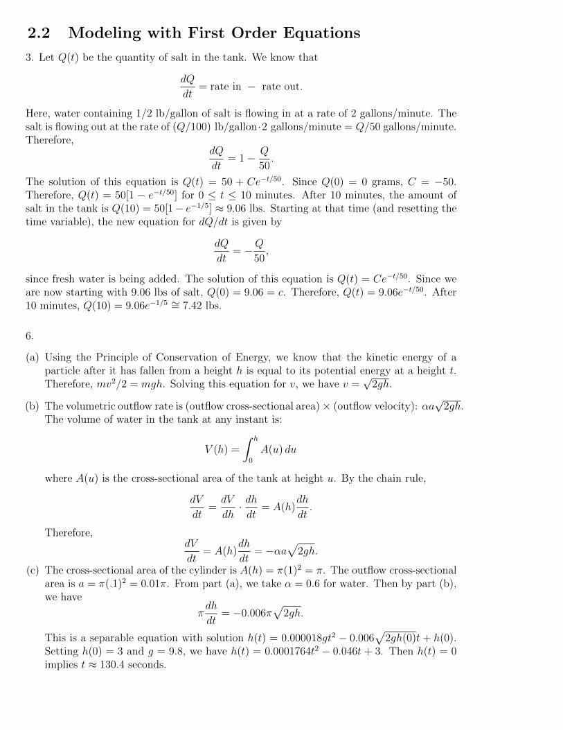
17.
(a) The solution of this separable equation is given by
u3 =u30
3αu30t+ 1
.
Since u0 = 2000, the specific solution is
u(t) =2000
(6t/125 + 1)1/3.
(b)
1000
1200
1400
1600
1800
2000
0 20 40 60 80 100 120 140 160 180 200t
(c) We look for τ so that u(τ) = 600. The solution of this equation is t ≈ 750.77 seconds.
18.
(a) The differential equation for Q is
dQ
dt= kr + P − Q(t)
Vr.
Therefore,
Vdc
dt= kr + P − c(t)r.
The solution of this equation is c(t) = k + P/r + (c0 − k − P/r)e−rt/V . Thereforelimt→∞ c(t) = k + P/r.
2.2. MODELING WITH FIRST ORDER EQUATIONS 63
The units on the left must match the units on the right. Since the units for tmg/v0 =
(s ·m/s2)/(m/s), the units cancel. As a result, we can conclude that kv0/mg is dimen-
sionless.
25.
(a) The equation of motion is given by mdv/dt = −kv −mg. The solution of this equation
is given by v(t) = −mg/k + (v0 +mg/k)e−kt/m.
(b) Applying L’Hospital’s rule, as k → 0, we have
limk→0
−mg/k + (v0 +mg/k)e−kt/m= v0 − gt.
(c)
limm→0
−mg/k + (v0 +mg/k)e−kt/m= 0.
26.
(a) The equation of motion is given by
mdv
dt= −6πµav + ρ�
4
3πa3g − ρ
4
3πa3g.
We can rewrite this equation as
v� +6πµa
mv =
4
3
πa3g
m(ρ� − ρ).
Multiplying by the integrating factor e6πµat/m, we have
(e6πµat/mv)� =4
3
πa3g
m(ρ� − ρ)e6πµat/m.
Integrating this equation, we have
v = e−6πµat/m
�2a2g(ρ� − ρ)
9µe6πµat/m + C
�
=2a2g(ρ� − ρ)
9µ+ Ce−6πµat/m.
Therefore, we conclude that the limiting velocity is vL = (2a2g(ρ� − ρ))/9µ.
(b) By the equation above, we see that the force exerted on the droplet of oil is given by
Ee = −6πµav + ρ�4
3πa3g − ρ
4
3πa3g.
If v = 0, then solving the above equation for e, we have
e =4πa3g(ρ� − ρ)
3E.
68 CHAPTER 2. FIRST ORDER DIFFERENTIAL EQUATIONS
by y(T ) = −160T + 267 + 125u sin(A) − (800 + 5u sin(A))[(u cos(A) − 70)/u cos(A)].Therefore, u and A must satisfy the inequality
800 ln
�u cos(A)− 70
u cos(A)
�+ 267 + 125u sin(A)− (800 + 5u sin(A))
�u cos(A)− 70
u cos(A)
�≥ 10.
31.
(a) Solving equation (i), we have y�(x) = [(k2−y)/y]1/2. The positive answer is chosen sincey is an increasing function of x.
(b) y = k2 sin2 t =⇒ dy/dt = 2k2 sin t cos t. Substituting this into the equation in part (a),we have
2k2 sin t cos tdt
dx=
cos t
sin t.
Therefore, 2k2 sin2 tdt = dx.
(c) Letting θ = 2t, we have k2 sin2(θ/2)dθ = dx. Integrating both sides, we have x(θ) =k2(θ − sin θ)/2. Further, using the fact that y = k2 sin2 t, we conclude that y(θ) =k2 sin2(θ/2) = k2(1− cos(θ))/2.
(d) From part (c), we see that y/x = (1− cos θ)/(θ− sin θ). If x = 1 and y = 2, the solutionof the equation is θ ≈ 1.401. Substituting that value of θ into either of the equations inpart (c), we conclude that k ≈ 2.193.
2.3 Differences between Linear and Nonlinear Equa-tions
1. Rewriting the equation as
y� +ln t
t− 3y =
2t
t− 3
and using Theorem 2.3.1, we conclude that a solution is guaranteed to exist in the interval0 < t < 3.
2. Rewriting the equation as
y� +1
t(t− 4)y = 0
and using Theorem 2.3.1, we conclude that a solution is guaranteed to exist in the interval0 < t < 4.
3. By Theorem 2.3.1, we conclude that a solution is guaranteed to exist in the intervalπ/2 < t < 3π/2.
4. Rewriting the equation as
y� +2t
4− t2y =
3t2
4− t2
2.3. DIFFERENCES BETWEEN LINEAR AND NONLINEAR EQUATIONS 69
and using Theorem 2.3.1, we conclude that a solution is guaranteed to exist in the interval−∞ < t < −2.
5. Rewriting the equation as
y� +2t
4− t2y =
3t2
4− t2
and using Theorem 2.3.1, we conclude that a solution is guaranteed to exist in the interval−2 < t < 2.
6. Rewriting the equation as
y� +1
ln ty =
cot t
ln tand using Theorem 2.3.1, we conclude that a solution is guaranteed to exist in the interval1 < t < π.
7. Using the fact that
f =t− y
2t+ 5y=⇒ fy = − 7t
(2t+ 5y)2,
we see that the hypothesis of Theorem 2.3.2 are satisfied as long as 2t+ 5y �= 0.
8. Using the fact that
f = (1− t2 − y2)1/2 =⇒ fy = − y
(1− t2 − y2)1/2,
we see that the hypothesis of Theorem 2.3.2 are satisfied as long as t2 + y2 < 1.
9. Using the fact that
f =ln |ty|
1− t2 + y2=⇒ fy =
1− t2 + y2 − 2y2 ln |ty|y(1− t2 + y2)2
,
we see that the hypothesis of Theorem 2.3.2 are satisfied as long as y, t �= 0 and 1−t2+y2 �= 0.
10. Using the fact that
f = (t2 + y2)3/2 =⇒ fy = 3y(t2 + y2)1/2,
we see that the hypothesis of Theorem 2.3.2 are satisfied for all t ∈ R.11. Using the fact that
f =1 + t2
3y − y2=⇒ fy = −(1 + t2)(3− 2y)
(3y − y2)2,
we see that the hypothesis of Theorem 2.3.2 are satisfied as long as y �= 0, 3.
12. Using the fact that
f =(cot t)y
1 + y=⇒ fy =
1
(1 + y)2,
we see that the hypothesis of Theorem 2.3.2 are satisfied as long as y �= −1, t �= nπ forn = 0, 1, 2 . . ..
74 CHAPTER 2. FIRST ORDER DIFFERENTIAL EQUATIONS
which can be written as (ertv)� = kert. The solution of this equation is given by v =
(k + cre−rt)/r. Then, using the fact that y = 1/v, we conclude that y = r/(k + cre−rt
).
30. Here n = 3. Therefore, v satisfies
v� + 2�v = 2σ.
This equation is linear with integrating factor e2�t. Its solution is given by v = (σ+c�e−2�t)/�.
Then, using the fact that y2 = 1/v, we see that y = ±√�/√σ + c�e−2�t.
31. Here n = 3. Therefore, v satisfies
v� + 2(Γ cos t+ T )v = 2.
This equation is linear with integrating factor e2(Γ sin t+Tt). Therefore,
�e2(Γ sin t+Tt)v
��= 2e2(à sin t+Tt)
which implies
v = 2e−2(Γ sin t+Tt)
� t
t0
exp(2(Γ sin s+ Ts)) ds+ ce−2(Γ sin t+Tt).
Then v = y−2implies y = ±
�1/v.
32. The solution of the initial value problem y� + 2y = 1 is y = 1/2 + ce−2t. For y(0) = 0,
we see that c = −1/2. Therefore, y(t) = 12(1− e−2t
) for 0 ≤ t ≤ 1. Then y(1) = 12(1− e−2
).
Next, the solution of y�+2y = 0 is given by y = ce−2t. The initial condition y(1) = 1
2(1−e−2)
implies ce−2=
12(1−e−2
). Therefore, c = 12(e
2−1) and we conclude that y(t) = 12(e
2−1)e−2t
for t > 1.
33. The solution of y� + 2y = 0 with y(0) = 1 is given by y(t) = e−2tfor 0 ≤ t ≤ 1. Then
y(1) = e−2. Then, for t > 1, the solution of the equation y� + y = 0 is y = ce−t
. Since we
want y(1) = e−2, we need ce−1
= e−2. Therefore, c = e−1
. Therefore, y(t) = e−1e−t= e−1−t
for t > 1.
34.
(a) Multiplying the equation by e� tt0
p(s) ds, we have
�e� tt0
p(s) dsy��
= e� tt0
p(s) dsg(t).
Integrating we have
e� tt0
p(s) dsy(t) = y0 +
� t
t0
e� st0
p(r) drg(s) ds,
which implies
y(t) = y0e−
� tt0
p(s) ds+
� t
t0
e−� ts p(r) drg(s) ds.
2.4. AUTONOMOUS EQUATIONS AND POPULATION DYNAMICS 75
(b) Assume p(t) ≥ p0 > 0 for all t ≥ t0 and |g(t)| ≤ M for all t ≥ t0. Therefore,
� t
t0
p(s) ds ≥� t
t0
p0 ds = p0(t− t0)
which implies
e−� tt0
p(s) ds ≤ e−� tt0
p0 ds = e−p0(t−t0) ≤ 1 for t ≥ t0.
Also,
� t
t0
e−� ts p(r) drg(s) ds ≤
� t
t0
e−� ts p(r) dr|g(s)| ds
≤� t
t0
e−p0(t−s)M ds
≤ Me−p0(t−s)
p0
����t
t0
= M
�1
p0− e−p0(t−t0)
p0
�
≤ M
p0
(c) Let p(t) = 2t+ 1 ≥ 1 for all t ≥ 0 and let g(t) = e−t2 . Therefore, |g(t)| ≤ 1 for all t ≥ 0.By the answer to part (a),
y(t) = e−� t0 (2s+1) ds +
� t
0
e−� ts (2r+1) dre−s2 ds
= e−(t2+t) + e−t2−t
� t
0
es ds
= e−t2 .
We see that y satisfies the property that y is bounded for all time t ≥ 0.
2.4 Autonomous Equations and Population Dynamics
1.
2.4. AUTONOMOUS EQUATIONS AND POPULATION DYNAMICS 77
0
-a/b
–3
–2
–1
0
1
2
3
y(t)
–2 –1 1 2t
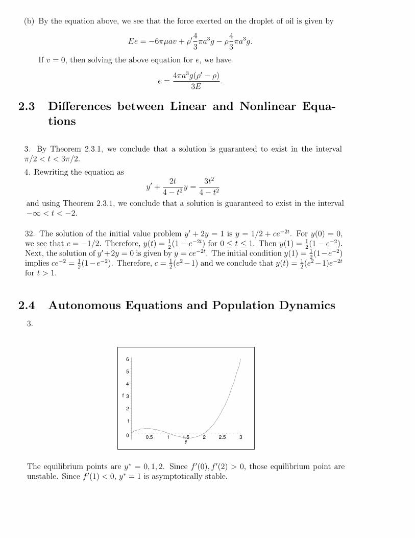
3.
0
1
2
3
4
5
6
f
0.5 1 1.5 2 2.5 3y
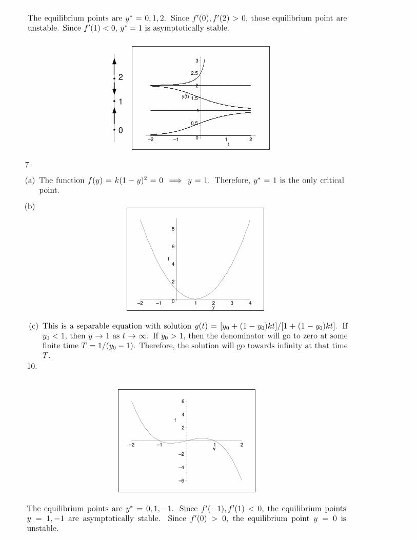
The equilibrium points are y∗ = 0, 1, 2. Since f �(0), f �(2) > 0, those equilibrium point areunstable. Since f �(1) < 0, y∗ = 1 is asymptotically stable.
1
0
2
0
0.5
1
1.5
2
2.5
3
y(t)
–2 –1 1 2t
4.
2.4. AUTONOMOUS EQUATIONS AND POPULATION DYNAMICS 77
0
-a/b
–3
–2
–1
0
1
2
3
y(t)
–2 –1 1 2t
3.
0
1
2
3
4
5
6
f
0.5 1 1.5 2 2.5 3y
The equilibrium points are y∗ = 0, 1, 2. Since f �(0), f �(2) > 0, those equilibrium point areunstable. Since f �(1) < 0, y∗ = 1 is asymptotically stable.
1
0
2
0
0.5
1
1.5
2
2.5
3
y(t)
–2 –1 1 2t
4.
2.4. AUTONOMOUS EQUATIONS AND POPULATION DYNAMICS 79
0
–3
–2
–1
0
1
2
3
y(t)
–2 –1 1 2t
6.
–0.8
–0.6
–0.4
–0.2
0
0.2
0.4
0.6
0.8
f
–4 –2 2 4y
The only equilibrium point is y∗ = 0. Since f �(0) < 0, the equilibrium point is asymptoticallystable.
0
–3
–2
–1
0
1
2
3
y(t)
–2 –1 1 2t
7.
(a) The function f(y) = k(1 − y)2 = 0 =⇒ y = 1. Therefore, y∗ = 1 is the only criticalpoint.
(b)
80 CHAPTER 2. FIRST ORDER DIFFERENTIAL EQUATIONS
0
2
4
6
8
f
–2 –1 1 2 3 4y
(c) This is a separable equation with solution y(t) = [y0 + (1 − y0)kt]/[1 + (1 − y0)kt]. Ify0 < 1, then y → 1 as t → ∞. If y0 > 1, then the denominator will go to zero at somefinite time T = 1/(y0 − 1). Therefore, the solution will go towards infinity at that timeT .
8.
–8
–6
–4
–2
f
–2 –1 1 2 3 4y
The only equilibrium point is y∗ = 1. Since f �(1) < 0. The equilibrium point is semistable.
1
–3
–2
–1
0
1
2
3
y(t)
–2 –1 1 2t
9.
2.4. AUTONOMOUS EQUATIONS AND POPULATION DYNAMICS 81
0
2
4
6
8
10
12
f
–2 –1 1 2y
The equilibrium points are y∗ = 0, 1,−1. Since f �(−1) < 0, y = −1 is asymptotically stable.Since f �(1) > 0, y = 1 is unstable. The equilibrium point y = 0 is semistable.
0
-1
1
–2
–1
0
1
2
3
y(t)
–2 –1 1 2t
10.
–6
–4
–2
2
4
6
f
–2 –1 1 2y
The equilibrium points are y∗ = 0, 1,−1. Since f �(−1), f �(1) < 0, the equilibrium pointsy = 1,−1 are asymptotically stable. Since f �(0) > 0, the equilibrium point y = 0 isunstable.
82 CHAPTER 2. FIRST ORDER DIFFERENTIAL EQUATIONS
0
-1
1
–2
–1
0
1
2
3
y(t)
–2 –1 1 2t
11.
–0.2
0
0.2
0.4
0.6
f
0.2 0.4 0.6 0.8 1 1.2 1.4 1.6 1.8 2y
The equilibrium points are y∗ = 0, b2/a2. Since f �(0) < 0, the equilibrium point y = 0 isasymptotically stable. Since f �(b2/a2) > 0, the equilibrium point y = b2/a2 is unstable.
0
b /a2 2
0
0.5
1
1.5
2
2.5
3
y(t)
–2 –1 1 2t
12.
2.4. AUTONOMOUS EQUATIONS AND POPULATION DYNAMICS 83
–14
–12
–10
–8
–6
–4
–2
0
2
4
f
–2 –1 1 2y
The equilibrium points are y∗ = 0, 2,−2. The equilibrium point y = 0 is semistable. Sincef �(−2) > 0, the equilibrium point y = −2 is unstable. Since f �(2) < 0, the equilibrium pointy = 2 is asymptotically stable.
0
-2
2
–3
–2
–1
0
1
2
3
y(t)
–2 –1 1 2t
13.
1
2
3
4
f
–1 –0.5 0.5 1 1.5 2y
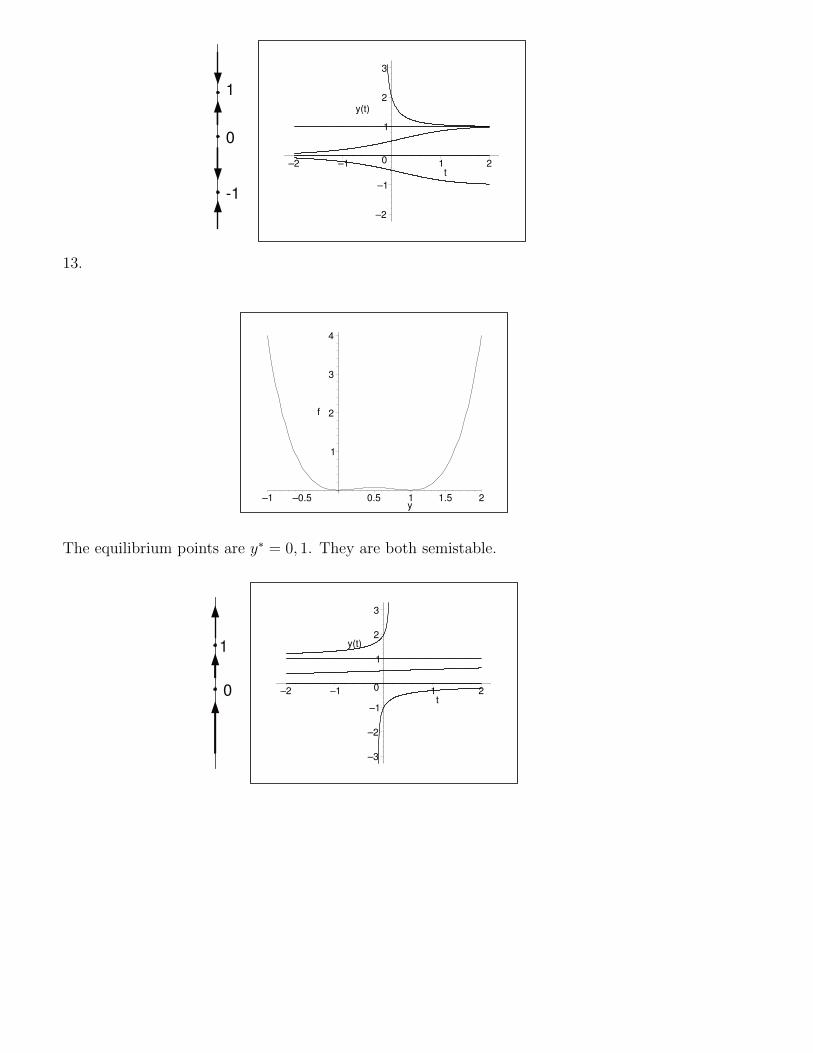
The equilibrium points are y∗ = 0, 1. They are both semistable.84 CHAPTER 2. FIRST ORDER DIFFERENTIAL EQUATIONS
0
1
–3
–2
–1
0
1
2
3
y(t)
–2 –1 1 2t
14.
(a) The equation is separable. Using partial fractions, it can be written as
�1
y+
1/K
1− y/K
�dy = rdt.
Integrating both sides and using the initial condition y0 = K/3, we know the solution ysatisfies
ln
����y
1− y/K
���� = rt+ ln
����K
2
���� .
To find the time τ such that y = 2y0 = 2K/3, we substitute y = 2K/3 and t = τ intothe equation above. Using the properties of logarithmic functions, we conclude thatτ = (ln 4)/r. If r = 0.025, then τ ≈ 55.452 years.
(b) Using the analysis from part (a), we know the general solution satisfies
ln
����y
1− y/K
���� = rt+ c.
The initial condition y0 = αK implies c = ln |αK/(1− α)|. Therefore,
ln
����y
1− y/K
���� = rt+ ln
����αK
1− α
���� .
In order to find the time T at which y(T ) = βK, we use the equation above. We concludethat
T = (1/r) ln |β(1− α)/α(1− β)|.
When α = 0.1, β = 0.9, r = 0.025, τ ≈ 175.78 years.
15.
(a) Below we sketch the graph of f for r = 1 = K.
2.4. AUTONOMOUS EQUATIONS AND POPULATION DYNAMICS 87
(d) Consider the equationy(1− (y/4))1/3
(y − 1)4/3= Ce−0.25t
found in part (c). If y0 = 2, then C = 22/3. Letting y(t) = 3.95 and solving for t, we seethat t ≈ 7.97. Similarly, if y0 = 6, we see that y ≤ 4.05 for t ≈ 7.97. For all initial data2 < y0 < 6, the conclusion also holds.
18.
(a) The surface area of the cone is given by
S = πa√h2 + a2 + πa2 = πa2(
�(h/a)2 + 1 + 1)
=πa2h
3· 3h
��(h/a)2 + 1 + 1
�
= cπ
�πa2h
3
�2/3
·�3a
πh
�2/3
= cπ
�3a
πh
�2/3
V 2/3.
Therefore, if the rate of evaporation is proportional to the surface area, then rate out =απ(3a/πh)2/3V 2/3. Therefore,
dV
dt= rate in− rate out
= k − απ
�3a
πh
�2/3 �π3a2h
�2/3
= k − απ
�3a
πh
�2/3
V 2/3.
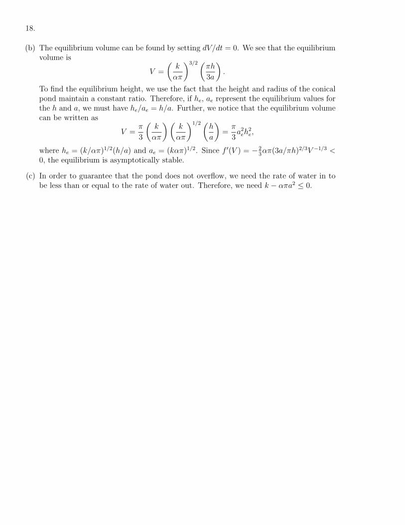
(b) The equilibrium volume can be found by setting dV/dt = 0. We see that the equilibriumvolume is
V =
�k
απ
�3/2 �πh
3a
�.
To find the equilibrium height, we use the fact that the height and radius of the conicalpond maintain a constant ratio. Therefore, if he, ae represent the equilibrium values forthe h and a, we must have he/ae = h/a. Further, we notice that the equilibrium volumecan be written as
V =π
3
�k
απ
��k
απ
�1/2 �h
a
�=
π
3a2eh
2e,
where he = (k/απ)1/2(h/a) and ae = (kαπ)1/2. Since f �(V ) = −23απ(3a/πh)
2/3V −1/3 <0, the equilibrium is asymptotically stable.
(c) In order to guarantee that the pond does not overflow, we need the rate of water in tobe less than or equal to the rate of water out. Therefore, we need k − απa2 ≤ 0.
2.4. AUTONOMOUS EQUATIONS AND POPULATION DYNAMICS 87
(d) Consider the equationy(1− (y/4))1/3
(y − 1)4/3= Ce−0.25t
found in part (c). If y0 = 2, then C = 22/3. Letting y(t) = 3.95 and solving for t, we seethat t ≈ 7.97. Similarly, if y0 = 6, we see that y ≤ 4.05 for t ≈ 7.97. For all initial data2 < y0 < 6, the conclusion also holds.
18.
(a) The surface area of the cone is given by
S = πa√h2 + a2 + πa2 = πa2(
�(h/a)2 + 1 + 1)
=πa2h
3· 3h
��(h/a)2 + 1 + 1
�
= cπ
�πa2h
3
�2/3
·�3a
πh
�2/3
= cπ
�3a
πh
�2/3
V 2/3.
Therefore, if the rate of evaporation is proportional to the surface area, then rate out =απ(3a/πh)2/3V 2/3. Therefore,
dV
dt= rate in− rate out
= k − απ
�3a
πh
�2/3 �π3a2h
�2/3
= k − απ
�3a
πh
�2/3
V 2/3.
(b) The equilibrium volume can be found by setting dV/dt = 0. We see that the equilibriumvolume is
V =
�k
απ
�3/2 �πh
3a
�.
To find the equilibrium height, we use the fact that the height and radius of the conicalpond maintain a constant ratio. Therefore, if he, ae represent the equilibrium values forthe h and a, we must have he/ae = h/a. Further, we notice that the equilibrium volumecan be written as
V =π
3
�k
απ
��k
απ
�1/2 �h
a
�=
π
3a2eh
2e,
where he = (k/απ)1/2(h/a) and ae = (kαπ)1/2. Since f �(V ) = −23απ(3a/πh)
2/3V −1/3 <0, the equilibrium is asymptotically stable.
(c) In order to guarantee that the pond does not overflow, we need the rate of water in tobe less than or equal to the rate of water out. Therefore, we need k − απa2 ≤ 0.