2156-5

Summer School in Cosmology

John Andrew PEACOCK

19 - 30 July 2010

University of Edinburgh Institute for Astronomy Royal Observatory

Blackford Hill, Edinburgh EH9 3HJ U.K.

Introduction to Cosmology

Introduction to Cosmology

ICTP Cosmology School; Trieste, July 2010

J.A. Peacock

Institute for Astronomy, University of Edinburgh

jap@roe.ac.uk http://www.roe.ac.uk/japwww

Outline

(1) Spacetime in an expanding universe FRW spacetime; Dynamics; Horizons; Observables

(2) Structure formation Inhomogeneities and Spherical model; Lagrangian approach; N-body simulations; Dark-matter haloes &mass function

(3) The hot big bang Thermal history; Freezeout; Relics; Nucleosynthesis; Recombination and last scattering

(4) Frontiers Initial condition problems; Vacuum energy; anthropics and the multiverse

1

Useful textbooks:

Dodelson: Modern Cosmology (Wiley)Kolb & Turner: The Early Universe (addison-Wesley)Lyth & Liddle: The Primordial Density Perturbation (CUP) Mukhanov: Physical Foundations of Cosmology (CUP)Peacock: Cosmological Physics (CUP)Peebles: Principles of Physical Cosmology (Princeton)Weinberg: Gravitation & Cosmology (Wiley)Weinberg: Cosmology (Oxford)

A very impressive web tutorial by Ned Wright may be helpful:http://www.astro.ucla.edu/~wright/cosmolog.htm

2

1 Spacetime in an expanding universe

These lectures concern the modern view of the overall properties of the universe. The heart of this view is that the universe is a dynamicalentity that has existed for only a finite period, and which reached its present state by evolution from initial conditions that are violentalmost beyond belief. Speculation about the nature of creation is older than history, of course, but the present view was arrived at onlyrather recently. A skeptic might therefore say that our current ideas may only be passing fashions. However, we are bold enough to saythat something is now really understood of the true nature of space and time on the largest scales. This is not to claim that we are anybrighter than those who went before; merely that we are fortunate enough to live when technology has finally revealed sufficient details ofthe universe for us to make a constrained theory. The resulting theory is strange, but it has been forced on us by observational facts thatwill not change.

The first key observation of the modern era was the discovery of the expanding universe. This is popularly credited to Edwin Hubblein 1929, but the honour arguably lies with Vesto Slipher, more than 10 years earlier. Slipher was measuring spectra of nebulae, and atthat time there was a big debate about what they were. Some thought that these extended blobs of light were clouds of gas, some thoughtthey were systems of stars at great distance. We now know that there are some of each, but stellar systems are in the majority away fromthe plane of the Milky Way. This was finally settled only in 1924, when Hubble discovered Cepheid variable stars in M31, establishingits distance of roughly 1 Mpc. More than a decade earlier, in 1913, Slipher had measured the spectrum of M31, and found that it wasapproaching the Earth at over 200 km s−1. Strangely, Slipher had the field to himself for another decade, by which time he had measuredDoppler shifts for dozens of galaxies: with only a few exceptions, these were redshifted. Furthermore, there was a tendency for the redshiftto be larger for the fainter galaxies. By the time Hubble came on the scene, the basics of relativistic cosmology were worked out andpredictions existed that redshift should increase with distance. It is hard to know how much these influenced Hubble, but by 1929 he hadobtained Cepheid distances for 24 galaxies with redshifts and claimed that these displayed a linear relationship:

v = Hd, (1)

citing theoretical predictions as a possible explanation. At the time, Hubble estimatedH � 500 km s−1Mpc−1, in part because his calibrationof Cepheid luminosities was in error. The best modern value is close to 70 km s−1Mpc−1.

3

1.1 The scale factor

A very simple model that yields Hubble’s law is what might be called the grenade universe: at time t = 0, set off a grenade in a bigempty space. Different bits of debris fly off at different speeds, and at time t will have reached a distance d = vt. This is Hubble’s law,with H = 1/t. We may therefore suspect that there was a violent event at a time about 1/H ago. This event is basically what we meanby the big bang: an origin of the expansion at a finite time in the past. The characteristic time of the expansion is called the Hubbletime, and takes the value

tH ≡ 9.78Gyr × (H/100 km s−1Mpc−1)−1. (2)

As we shall see, this is not the actual age of the universe, since gravity stops the expansion proceeding at uniform speed.

The grenade universe is a neat idea, but it can leave you with a seriously flawed view of the universe. First, the model has a centre,where we are presumed to live; second, the model has an edge – and the expansion proceeds to fill empty space. The real situation seemsto be that we do not live in a special place, nor is there an edge to the galaxy distribution.

It is easy enough to think of an alternative model, in which the Earth need not be at the centre of the universe. Consider a distributionof galaxies that is made to expand uniformly, in the same way as if a picture of the pattern was undergoing continuous magnification.Mathematically, this means that all position vectors at time t are just scaled versions of their values at a reference time t0:

x(t) = R(t)x(t0). (3)

Differentiating this with respect to t gives

x(t) = R(t)x(t0) = [R(t)/R(t)]x(t), (4)

or a velocity proportional to distance, as required. Writing this relation for two points 1 & 2 and subtracting shows that this expansionappears the same for any choice of origin: everyone is the centre of the universe:

[x2(t)− x1(t)] = H(t) [x2(t)− x1(t)]; H(t) = R(t)/R(t). (5)

This shows that Hubble’s constant can be identified with R(t)/R(t), and that in general it is not a constant, but something that can changewith time.

4

1.2 Cosmological spacetime

One of the fundamentals of a cosmologist’s toolkit is to be able to assign coordinates to events in the universe. We need a large-scale notionof space and time that allows us to relate observations we make here and now to physical conditions at some location that is distant in timeand space. The starting point is the relativistic idea that spacetime must have a metric: the equivalence principle says that conditionsaround our distant object will be as in special relativity (if it is freely falling), so there will be the usual idea of the interval or propertime between events, which we want to rewrite in terms of our coordinates:

−ds2 = c2dτ2 = c2dt′2 − dx′2 − dy′2 − dz′2 = gμνdxμdxν . (6)

Here, dashed coordinates are local to the object, undashed are the global coordinates we use. As usual, the Greek indices run from 0 to3. Note the ambiguity in defining the sign of the squared interval. The matrix gμν is the metric tensor, which is found in principle bysolving Einstein’s gravitational field equations. A simpler alternative, which fortunately matches the observed universe pretty well, is toconsider the most symmetric possibilities for the metric.

de sitter space Again according to Einstein, any spacetime with non-zero matter content must have some spacetime curvature, i.e.the metric cannot have the special relativity form diag(+1,−1,−1,−1). This curvature is something intrinsic to the spacetime, and doesnot need to be associated with extra spatial dimensions; these are nevertheless a useful intuitive way of understanding curved spaces suchas the 2D surface of a 3D sphere. To motivate what is to come, consider the higher-dimensional analogue of this surface: something thatis almost a 4D (hyper)sphere in Euclidean 5D space:

x2 + y2 + z2 + w2 − v2 = A2 (7)

where the metric is

ds2 = dx2 + dy2 + dz2 + dw2 − dv2. (8)

Effectively, we have made one coordinate imaginary because we know we want to end up with the 4D spacetime signature.

5

This maximally symmetric spacetime is known as de Sitter space. It looks like a static spacetime, but relativity can be deceptive,as the interpretation depends on the coordinates you choose. Suppose we re-express things using the analogues of polar coordinates:

v = A sinhα

w = A coshα cosβ

z = A coshα sinβ cos γ

y = A coshα sinβ sin γ cos δ

x = A coshα sinβ sin γ sin δ.

(9)

This has the advantage that it is an orthogonal coordinate system: a vector such as eα = ∂(x, y, z, w, v)/∂α is orthogonal to all the otherei (most simply seen by considering eδ and imagining continuing the process to still more dimensions). The squared length of the vectoris just the sum of |eαi

|2 dα2i , which makes the metric into

ds2 = −A2dα2 +A2 cosh2 α(dβ2 + sin2(β)[dγ2 + sin2 γdδ2]

), (10)

which by an obvious change of notation becomes

c2dτ2 = c2dt2 −A2 cosh2(t/A)(dr2 + sin2(r)[dθ2 + sin2 θdφ2]

). (11)

Now we have a completely different interpretation of the metric:

(interval)2= (time interval)

2 − (scale factor)2(comoving interval)

2. (12)

There is a universal cosmological time, which is the ticking of clocks at constant comoving radius r and constant angle on thesky. The spatial part of the metric expands with time, so that particles at constant r recede from the origin, and must thus suffer aDoppler redshift. This of course presumes that constant r corresponds to the actual trajectory of a free particle, which we have not proved– although it is true.

6

Historically, de Sitter space was extremely important in cosmology, although it was not immediately clear that the model is non-static.The metric was first derived by de Sitter in the following form:

c2dτ2 = (1− r′2/R2) c2dt′2 − (1− r′2/R2)−1dr′2 − r′2 dψ2, (13)

where now r is a proper radius, and R is a curvature radius. To show that this is the same metric, a fair bit of tedious algebra is required.The starting point is to identify the transverse parts involving dψ2, so that r′ = A cosh(t/A) sin r, which can be differentiated to yielddr′ = sinh(t/A) sin r dt + A cosh(t/A) cos r dr. Squaring this yields terms that include an undesired cross term involving dr dt. This canbe eliminated by writing dt′ = a dt + b dr, where a & b are two spacetime functions. With the right choice of a & b, we get the static deSitter metric, with R = cA.

It is not at all obvious that there is anything expanding about the second form, and historically this remained obscure for some time.Although it was eventually concluded (in 1923, by Weyl) that one would expect a redshift that increased linearly with distance in de Sitter’smodel, this was interpreted as measuring the constant radius of curvature of spacetime, R. By this time, Slipher had already establishedthat most galaxies were redshifted. Hubble’s 1929 ‘discovery’ of the expanding universe was explicitly motivated by the possibility of findingthe ‘de Sitter effect’ (although we now know that his sample was too shallow to be able to detect it reliably).

In short, it takes more than just the appearance of R(t) in a metric to prove that something is expanding. That this is the correctway to think about things only becomes apparent when we take a local (and thus Newtonian, thanks to the equivalence principle) look atparticle dynamics. Then it becomes clear that a static distribution of test particles is impossible in general, so that it makes more sense touse an expanding coordinate system defined by the locations of such a set of particles.

1.3 The Robertson-Walker metric

The de Sitter model is only one example of an isotropically expanding spacetime, and we need to make the idea general, which involvesweakening the symmetry – but only slightly.

fundamental observers As with de Sitter space, we assume a cosmological time t, which is the time measured by the clocks ofthese observers – i.e. t is the proper time measured by an observer at rest with respect to the local matter distribution (these characters are

7

usually termed fundamental observers). We can envisage them as each sitting on a different galaxy, and so receding from each otherwith the general expansion. Actually this is not quite right, since each galaxy has a peculiar velocity with respect to its neighbours ofa few hundred km s−1. We really need to deal with an idealized universe where the matter density is uniform.

The fundamental observers give us a way of defining a universal time coordinate, even though relativity tells us that such a thing isimpossible in general. It makes sense that such a universal time exists if we accept that we are looking for models that are homogeneous,so that there are no preferred locations. This is obvious in de Sitter space: because it derives from a 4-sphere, all spacetime points aremanifestly equivalent: the spacetime curvature and hence the matter density must be a constant. The next step is to to weaken this so thatconditions can change with time, but are uniform at a given time. A cosmological time coordinate can then be defined and synchronizedby setting clocks to a reference value at some standard density.

isotropy and homogeneity So far, cosmological time is not very useful, since it is not so easy to arrange to sychronize all theclocks of the different observers. The way this problem is solved is because we will consider mass distributions with special symmetries.The Hubble expansion that we see is isotropic – the same in all directions. Also, all large-scale properties of the universe such as thedistribution of faint galaxies on the sky seem to be accurately isotropic. If this is true for us, we can make a plausible guess, calledthe cosmological principle: that conditions will be seen as isotropic around each observer. If this holds (and it can be checkedobservationally, so it’s not just an article of religious faith), then we can prove that the mass distribution must be homogeneous – i.e.

the same density everywhere at a given time. The proof is very easy: just draw a pair of intersecting spheres about two observers. Thedensity on each sphere is a constant by isotropy, and it must be the same constant since they intersect.

Homogeneity is what allows cosmological time to be useful globally rather than locally: because the clocks can be synchronized ifobservers set their clocks to a standard time when the universal homogeneous density reaches some given value.

metrics on spheres We now need a way of describing the global structure of space and time in such a homogeneous space. Locally,we have said that things look like special relativity to a fundamental observer on the spot: for them, the proper time interval between twoevents is c2dτ2 = c2dt2− dx2− dy2− dz2. Since we use the same time coordinate as they do, our only difficulty is in the spatial part of themetric: relating their dx etc. to spatial coordinates centred on us.

8

E

A

B

C

D

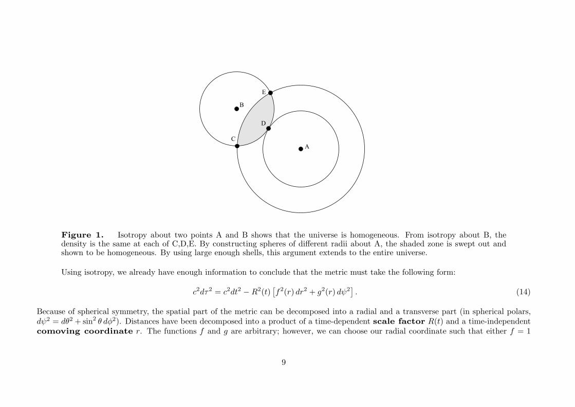
Figure 1. Isotropy about two points A and B shows that the universe is homogeneous. From isotropy about B, thedensity is the same at each of C,D,E. By constructing spheres of different radii about A, the shaded zone is swept out andshown to be homogeneous. By using large enough shells, this argument extends to the entire universe.

Using isotropy, we already have enough information to conclude that the metric must take the following form:

c2dτ2 = c2dt2 −R2(t)[f2(r) dr2 + g2(r) dψ2

]. (14)

Because of spherical symmetry, the spatial part of the metric can be decomposed into a radial and a transverse part (in spherical polars,dψ2 = dθ2 + sin2 θ dφ2). Distances have been decomposed into a product of a time-dependent scale factor R(t) and a time-independentcomoving coordinate r. The functions f and g are arbitrary; however, we can choose our radial coordinate such that either f = 1

9

or g = r2, to make things look as much like Euclidean space as possible. The problem is solved if we can only determine the form of theremaining function.

To get some feeling for the general answer, it should help to think first about a simpler case: the metric on the surface of a sphere.A balloon being inflated is a common popular analogy for the expanding universe, and it will serve as a two-dimensional example of a spaceof constant curvature. If we call the polar angle in spherical polars r instead of the more usual θ, then the element of length dσ on thesurface of a sphere of radius R is

dσ2 = R2(dr2 + sin2 r dφ2

). (15)

It is possible to convert this to the metric for a 2-space of constant negative curvature by the device of considering an imaginaryradius of curvature, R→ iR. If we simultaneously let r → ir, we obtain

dσ2 = R2(dr2 + sinh2 r dφ2

). (16)

These two forms can be combined by defining a new radial coordinate that makes the transverse part of the metric look Euclidean:

dσ2 = R2

(dr2

1− kr2 + r2 dφ2

), (17)

where k = +1 for positive curvature and k = −1 for negative curvature.An isotropic universe has the same form for the comoving spatial part of its metric as the surface of a sphere. This is no accident,

since it it possible to define the equivalent of a sphere in higher numbers of dimensions, and the form of the metric is always the same.Let’s start with the case of the surface of a sphere, supposing that we were ants, with no concept of the third dimension away from thesurface of the sphere. A higher-dimensional generalization of the circle, x2 + y2 = R2, would be Pythagoras with one extra coordinate:

x2 + y2 + z2 = R2. (18)

10

We can always satisfy this by defining some angles:

z = R cos θ

y = R sin θ sinφ

x = R sin θ cosφ.

(19)

3D beings recognize these as the usual polar angles, but we don’t need this insight – other angles could have been defined that would workjust as well. An element of length in this Euclidean space will be

dσ2 = dx2 + dy2 + dz2, (20)

and we can express this in terms of the angles using

dx = R(cos θ cosφdθ − sin θ sinφdφ)

dy = R(cos θ sinφdθ + sin θ cosφdφ)

dz = R(− sin θ dθ).(21)

Multiplying everything out, we get dσ2 = R2(dθ2+sin2 θ dφ2). This is the expected result, but no geometrical insight was required beyondthe element of length in Euclidean space.

Moving up one dimension, a 3-sphere embedded in four-dimensional Euclidean space would be defined as the coordinate relationx2 + y2 + z2 + w2 = R2. Now define the equivalent of spherical polars and write w = R cosα, z = R sinα cosβ, y = R sinα sinβ cos γ,x = R sinα sinβ sin γ, where α, β and γ are three arbitrary angles. Differentiating with respect to the angles gives a four-dimensional vector(dx, dy, dz, dw), and we need the modulus of this vector. We could work this out by brute force as before, by evaluating dx2+dy2+dz2+dw2;a slightly easier route is to consider the vectors generated by increments in dα etc.:

eα = dαR ( cosα sinβ sin γ, cosα sinβ cos γ, cosα cosβ, − sinα )eβ = dβ R ( sinα cosβ sin γ, sinα cosβ cos γ, − sinα sinβ, 0 )eγ = dγ R ( sinα sinβ cos γ, − sinα sinβ sin γ, 0, 0 ).

(22)

11

These are easily checked to be orthogonal, so the squared length of the vector is just |eα|2 + |eβ |2 + |eγ |2, which gives

|(dx, dy, dz, dw)|2 = R2[dα2 + sin2 α (dβ2 + sin2 β dγ2)

]. (23)

This is the metric for the case of positive spatial curvature, if we relabel α → r and (β, γ) → (θ, φ) – the usual polar angles. We couldwrite the angular part just in terms of the angle dψ that separates two points on the sky, dψ2 = dθ2 + sin2 θ dφ2, in which case the metricis the same form as for the surface of a sphere. This was inevitable: the hypersurface x2 + y2 + z2 + w2 = R2 always allows two points tobe chosen to have w = 0 (the first by choice of origin; the second via rotation), so that their separation is that of two points on the surfaceof a sphere.

It is possible to deal with the 3-sphere without introducing angles via the following trick: write x2+y2+z2+w2 = R2 as r2+w2 = R2,so that w dw = −r dr, implying dw2 = r2dr2/(R2 − r2). The spatial part of the metric is therefore just

dσ2 = dx2 + dy2 + dz2 + r2dr2/(R2 − r2). (24)

Introducing 3D polar coordinates, we have

dx2 + dy2 + dz2 = dr2 + r2(dθ2 + sin2 θ dφ2

), (25)

so that we get the spatial part of the RW metric in its second form:

dσ2 =dr2

1− r2/R2+ r2

(dθ2 + sin2 θ dφ2

). (26)

To convert to the form we had previously, we should replace r here by R sin r. In making this argument, remember the subtlety that (x, y, z)are coordinates in the embedding space, which differ from the coordinates that a 3D observer would erect in their vicinity; to clarify things,imagine how the same arguments work for a sphere, where the two points of interest can always be chosen to lie along a great circle.

This k = +1 metric describes a closed universe, in which a traveller who sets off along a trajectory of fixed β and γ will eventuallyreturn to their starting point (when α = 2π). In this respect, the positively curved 3D universe is identical to the case of the surface of asphere: it is finite, but unbounded. By contrast, if we define a space of negative curvature via R → iR and α → iα, then sinα → i sinhα

12

and cosα→ coshα (so that x, y, z stay real, as they must). The new angle α can increase without limit, and (x, y, z) never return to theirstarting values. The k = −1 metric thus describes an open universe of infinite extent.

summary of the rw metric We can now sum up the overall metric, where the time part just comes from cosmological time:c2dτ2 = c2dt2 − dσ2. The result is the Robertson–Walker metric (RW metric), which may be written in a number of different ways.The most compact forms are those where the comoving coordinates are dimensionless. Define the very useful function

Sk(r) =

⎧⎨⎩sin r (k = 1)sinh r (k = −1)r (k = 0).

(27)

The metric can now be written in the preferred form that we shall use throughout:

c2dτ2 = c2dt2 −R2(t)[dr2 + S2

k(r) dψ2]. (28)

The most common alternative is to use a different definition of comoving distance, Sk(r)→ r, so that the metric becomes

c2dτ2 = c2dt2 −R2(t)

(dr2

1− kr2 + r2dψ2

). (29)

There should of course be two different symbols for the different comoving radii, but each is often called r in the literature. We will normallystick with the first form. Alternatively, one can make the scale factor dimensionless, defining

a(t) ≡ R(t)

R0, (30)

so that a = 1 at the present.

Lastly, note that, although comoving distance is dimensionless in the above conventions, it is normal in the cosmological literatureto discuss comoving distances with units of length (e.g. Mpc). This is because one normally considers the combination R0r or R0Sk(r) –i.e. these are the proper lengths that correspond to the given comoving separation at the current time.

13

1.4 Light propagation and redshift

Light follows trajectories with zero proper time (null geodesics). The radial equation of motion therefore integrates to

r =

∫c dt/R(t). (31)

The comoving distance is constant, whereas the domain of integration in time extends from temit to tobs; these are the times of emissionand reception of a photon. Thus dtemit/dtobs = R(temit)/R(tobs), which means that events on distant galaxies time-dilate. This dilationalso applies to frequency, so

νemit

νobs≡ 1 + z =

R(tobs)

R(temit). (32)

In terms of the normalized scale factor a(t) we have simply a(t) = (1+ z)−1. So just by observing shifts in spectral lines, we can learn howbig the universe was at the time the light was emitted. This is the key to performing observational cosmology.

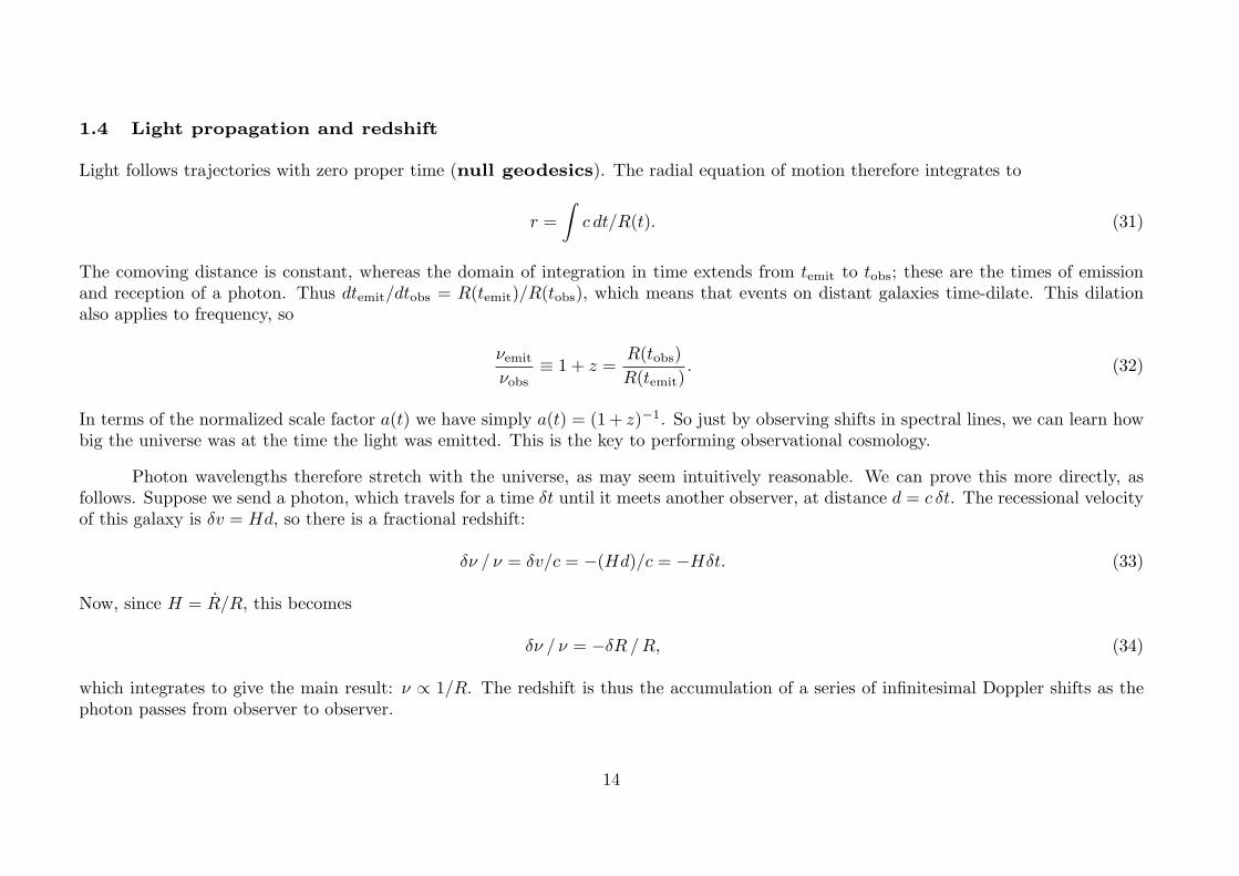
Photon wavelengths therefore stretch with the universe, as may seem intuitively reasonable. We can prove this more directly, asfollows. Suppose we send a photon, which travels for a time δt until it meets another observer, at distance d = c δt. The recessional velocityof this galaxy is δv = Hd, so there is a fractional redshift:

δν / ν = δv/c = −(Hd)/c = −Hδt. (33)

Now, since H = R/R, this becomes

δν / ν = −δR /R, (34)

which integrates to give the main result: ν ∝ 1/R. The redshift is thus the accumulation of a series of infinitesimal Doppler shifts as thephoton passes from observer to observer.

14

However, this is not the same as saying that the redshift tells us how fast the observed galaxy is receding. A common but incorrectapproach is to use the special-relativistic Doppler formula and write

1 + z =

√1 + v/c

1− v/c . (35)

Indeed, it is all too common to read of the latest high-redshift quasar as “receding at 95% of the speed of light”. The reason the redshiftcannot be interpreted in this way is because a non-zero mass density must cause gravitational redshifts. If we want to think of the redshiftglobally, it is better to stick with the ratio of scale factors. However, one can get somewhere by considering the distance-redshift relationto quadratic order. At this level, spacetime curvature is unimportant: r and Sk(r) differ only at order r

3, so we are spared the difficultquestion as to which is the better definition of distance. Now consider a photon that we receive from distance d: drawing a sphere aroundus, it is clear that this photon falls towards us through a gravitational potential GM/d, which is proportional to d2. Thus there is agravitational blueshift contribution to z that is quadratic in distance.

Finally, note that the law that frequency of photons scales as 1/R actually applies to the momentum of all particles – relativistic ornot: we just need to consider applying a small boost to the 4-momentum Pμ and remember that P/E is the particle velocity. Thinkingof quantum mechanics, the de Broglie wavelength is λ = 2πh/p, so this scales with the side of the universe, as if the waves were standingwaves trapped in a box (see figure 2).

1.5 Cosmological dynamics

Thus almost everything in cosmology reduces to knowing R(t). The equation of motion for the scale factor is something that can nearly beunderstood by a Newtonian approach, and this is the approach we shall try to adopt, but it is worth outlining the steps needed in a morerigorous approach.

What we need to do is insert the RW metric, gμν into Einstein’s field equations:

Gμν ≡ Rμν −Rgμν/2 = −(8πG/c4)Tμν , (36)

15

Figure 2. Suppose we trap some radiation inside a box with silvered sides, that expands with the universe. At least foran isotropic radiation field, the photons trapped in the box are statistically equivalent to any that would pass into this spacefrom outside. Since the walls expand at v � c for a small box, it is easily shown that the Doppler shift maintains an adiabaticinvariant, which is the ratio of wavelength to box side, and so radiation wavelengths increase as the universe expands. Thisargument also applies to quantum-mechanical standing waves: momentum declines as a(t)−1.

where the Ricci tensor and scalar derive from the Riemann tensor

Rμαβγ =

∂Γμαγ

∂xβ− ∂Γμ

αβ

∂xγ+ Γμ

σβΓσγα − Γμ

σγΓσβα. (37)

via

Rαβ = Rμαβμ

R = Rμμ = gμνRμν

(38)

(other conventions are possible). The components of the connection are

Γαλμ =

12g

αν

(∂gμν

∂xλ+∂gλν

∂xμ− ∂gμλ

∂xν

). (39)

16

So in principle we just have to perform the necessary differentiations, remembering clearly that the coordinates being used are not Cartesian:

xμ = (ct, r, θ, φ). (40)

But what is the energy-momentum tensor, Tμν? For an isotropic fluid, it must be Tμν = (ρ + p)UμUν − pgμν . Since three ofour coordinates are unchanging comoving coordinates, Uμ ∝ (1, 0, 0, 0). Things can be made simpler if we lower one index, so thatTμ

ν = diag(ρc2,−p,−p,−p), as in special relativity, because gμν = diag(1, 1, 1, 1), independent of whether the metric is curved. The two

independent Einstein equations are

G00 = 3(R2 + k)/R2 = 8πGρ

G11 = (2RR+ R2 + k)/R2 = 8πGp,

(41)

which are two forms of the Friedmann equation.

the friedmann equation The equation of motion for the scale factor resembles Newtonian conservation of energy for a particle atthe edge of a uniform sphere of radius R:

R2 − 8πG

3ρR2 = −kc2. (42)

This is almost obviously true, since the Newtonian result that the gravitational field inside a uniform shell is zero does still hold in generalrelativity, and is known as Birkhoff’s theorem. But there are some surprises hidden here. This energy-like equation can be turnedinto a force-like equation by differentiating with respect to time:

R = −4πGR(ρ+ 3p/c2)/3. (43)

To deduce this, we need to know ρ, which comes from conservation of energy:

d[ρc2R3] = −pd[R3]. (44)

17

The surprising factor here is the occurrence of the active mass density ρ+3p/c2. This is here because the weak-field form of Einstein’sgravitational field equations is

∇2Φ = 4πG(ρ+ 3p/c2). (45)

The extra term from the pressure is important. As an example, consider a radiation-dominated fluid – i.e. one whose equation ofstate is the same as that of pure radiation: p = u/3, where u is the energy density. For such a fluid, ρ+ 3p/c2 = 2ρ, so its gravity is twiceas strong as we might have expected.

But the greatest astonishment in the Friedmann equation is the term on the rhs. This is related to the curvature of spacetime, andk = 0,±1 is the same integer that is found in the RW metric. This cannot be completely justified without the Field Equations, but theflat k = 0 case is readily understood. Write the energy-conservation equation with an arbitrary rhs, but divide through by R2:

H2 − 8πG

3ρ =

const

R2. (46)

Now imagine holding the observables H and ρ constant, but let R → ∞; this has the effect of making the rhs of the Friedmann equationindistinguishable from zero. Looking at the metric with k = 0, R→∞ with Rr fixed implies r → 0, so the difference between Sk(r) and rbecomes negligible and we have in effect the k = 0 case.

There is thus a critical density that will yield a flat universe,

ρc =3H2

8πG. (47)

It is common to define a dimensionless density parameter as the ratio of density to critical density:

Ω ≡ ρ

ρc=8πGρ

3H2. (48)

18

The current value of such parameters should be distinguished by a zero subscript. In these terms, the Friedmann equation gives the presentvalue of the scale factor:

R0 =c

H0[(Ω0 − 1)/k]−1/2, (49)

which diverges as the universe approaches the flat state with Ω = 1. In practice, Ω0 is such a common symbol in cosmological formulae,that it is normal to omit the zero subscript. We can also define a dimensionless (current) Hubble parameter as

h ≡ H0

100 km s−1Mpc−1, (50)

in terms of which the current density of the universe is

ρ0 = 1.878× 10−26 Ωh2 kgm−3

= 2.775× 1011 Ωh2 M�Mpc−3.

(51)

1.6 Vacuum energy in cosmology

The discussion so far is general, and independent of the detailed constituents of the universe. But before proceeding, it is worth an aside onwhat is in many ways the key factor in determining the expansion: the energy density of empty space. This is an idea that was introducedby Einstein, soon after he arrived at the theory of general relativity. However, the main argument has a much older motivation, as follows.

einstein’s static universe The expanding universe is the solution to a problem that goes back to Newton. After expounding theidea of universal gravitation, he was asked what would happen to mass in an infinite space. If all particles with mass attracted each other,how could the heavens be stable (as they apparently were, give or take the motions of planets)? In 1917, Einstein was still facing the sameproblem, but he thought of an ingenious solution. Gravitation can be reduced to the potential that solved Poisson’s equation: ∇2Φ = 4πGρ.

19

Einstein argued by symmetry that, in a universe where the density ρ is constant, the potential Φ must be also (so that the accelerationa = −∇∇∇∇∇∇∇∇∇∇∇∇∇Φ vanishes everywhere). Since this doesn’t solve Poisson’s equation, he proposed that it should be replaced:

∇2Φ+ λΦ = 4πGρ, (52)

where λ is a new constant of nature, called the cosmological constant in its relativistic incarnation. This clearly lets us have a staticmodel, with Φ = 4πGρ/λ.

The modern way of writing this is to take the new term onto the other side, defining ρrep = λΦ/4πG:

∇2Φ = 4πG(ρ− ρrep), (53)

i.e. to interpret it as a constant repulsive density, with antigravity properties. By this definition, ρ = ρrep, so the rhs vanishes, and therepulsive density cancels the effect of normal matter. This repulsion would have to be an intrinsic property of the vacuum, since it has tobe present when all matter is absent. This may sound like a really stupid idea, but in fact it is the basis of much of modern cosmology.

Interestingly, Einstein’s neat argument is not really consistent with the relativistic generalization, and he might equally well havewritten ∇2Φ + λ = 4πGρ; this still allows a constant-potential solution, although the absolute value of potential cannot be found. Thisdoes not matter, since only gradients will cause forces.

When looked at as a vacuum repulsion, we can see that Einstein’s idea couldn’t work. Suppose we increase the matter densityin some part of space a little: the mutual attraction of normal matter goes up, but the vacuum repulsion stays constant and doesn’tcompensate. In short, Einstein’s static universe is unstable, and must either expand or contract. We can stretch this only a little to saythat the expanding universe could have been predicted by Newton.

energy density of the vacuum Nevertheless, vacuum energy is central to modern cosmology. How can a vacuum have a non-zeroenergy density? Surely this is zero by definition in a vacuum? It turns out that this need not be true. What we can say is that, if thevacuum has a non-zero energy density, it must also have a non-zero pressure, with a negative-pressure equation of state:

pvac = −ρvac c2. (54)

20

In this case, ρc2 + 3p is indeed negative: a positive vacuum density will act to cause a large-scale repulsion.

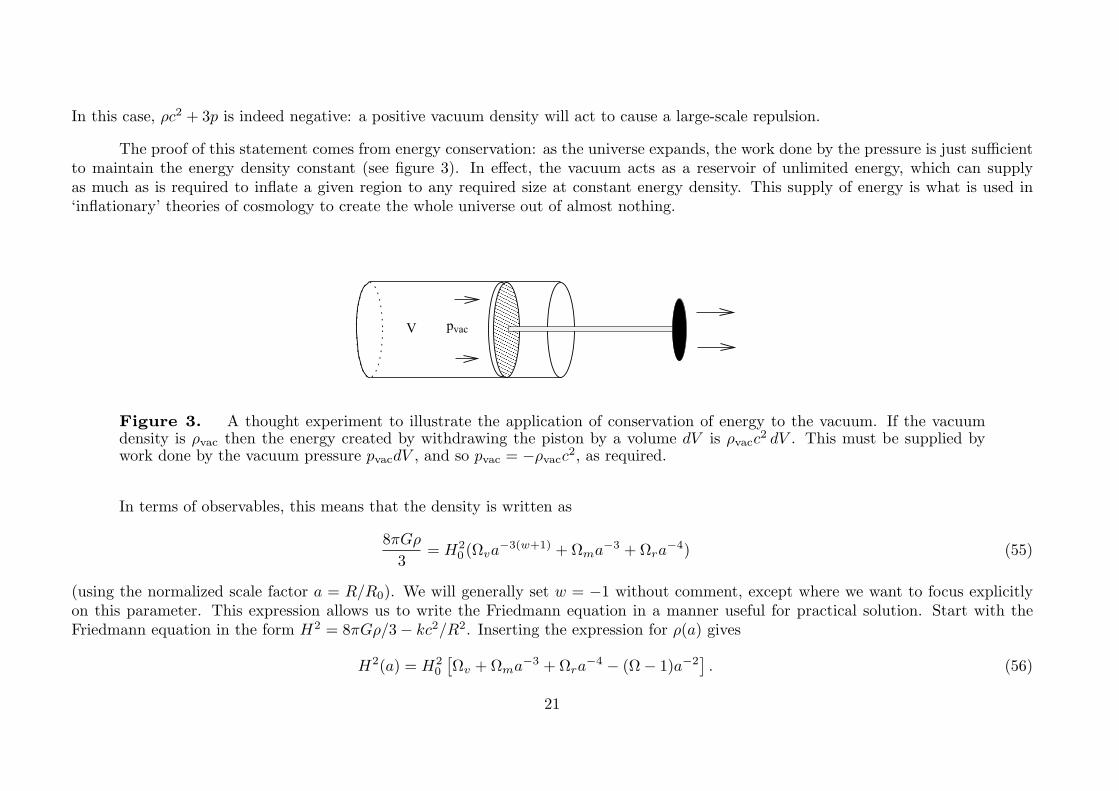
The proof of this statement comes from energy conservation: as the universe expands, the work done by the pressure is just sufficientto maintain the energy density constant (see figure 3). In effect, the vacuum acts as a reservoir of unlimited energy, which can supplyas much as is required to inflate a given region to any required size at constant energy density. This supply of energy is what is used in‘inflationary’ theories of cosmology to create the whole universe out of almost nothing.

������������������������������

������������������������������

V vacp

Figure 3. A thought experiment to illustrate the application of conservation of energy to the vacuum. If the vacuumdensity is ρvac then the energy created by withdrawing the piston by a volume dV is ρvacc

2 dV . This must be supplied bywork done by the vacuum pressure pvacdV , and so pvac = −ρvacc

2, as required.

In terms of observables, this means that the density is written as

8πGρ

3= H2

0 (Ωva−3(w+1) +Ωma

−3 +Ωra−4) (55)

(using the normalized scale factor a = R/R0). We will generally set w = −1 without comment, except where we want to focus explicitlyon this parameter. This expression allows us to write the Friedmann equation in a manner useful for practical solution. Start with theFriedmann equation in the form H2 = 8πGρ/3− kc2/R2. Inserting the expression for ρ(a) gives

H2(a) = H20

[Ωv +Ωma

−3 +Ωra−4 − (Ω− 1)a−2

]. (56)

21

This equation is in a form that can be integrated immediately to get t(a). This is not possible analytically in all cases, nor can we alwaysinvert to get a(t), but there are some useful special cases worth knowing. Mostly these refer to the flat universe with total Ω = 1.Curvature can always be neglected at sufficiently early times, as can vacuum density (except that the theory of inflation postulates thatthe vacuum density was very much higher in the very distant past). The solutions look simplest if we appreciate that normalization to thecurrent era is arbitrary, so we can choose a = 1 to be at a convenient point where the densities of two main components cross over. Also,the Hubble parameter at that point (H∗) sets a characteristic time, from which we can make a dimensionless version τ ≡ tH∗.

1.7 Solving the Friedmann equation

models with general equations of state To solve the Friedmann equation, we need to specify the matter content of theuniverse, and there are two obvious candidates: pressureless nonrelativistic matter, and radiation-dominated matter. These have densitiesthat scale respectively as a−3 and a−4. The first two relations just say that the number density of particles is diluted by the expansion,with photons also having their energy reduced by the redshift. We can be more general, and wonder if the universe might contain anotherform of matter that we have not yet considered. How this varies with redshift depends on its equation of state. If we define the parameter

w ≡ p/ρc2, (57)

then conservation of energy says

d(ρc2V ) = −p dV ⇒ d(ρc2V ) = −wρc2 dV ⇒ d ln ρ/d ln a = −3(w + 1), (58)

so

ρ ∝ a−3(w+1) (59)

if w is constant. Pressureless nonrelativistic matter has w = 0, radiation has w = 1/3, and vacuum energy has w = −1.

22

matter and radiation Using dashes to denote d/d(t/τ), we have a′2= (a−2 + a−1)/2, which is simply integrated to yield

τ =2√2

3

(2 + (a− 2)

√1 + a

). (60)

This can be inverted to yield a(τ), but the full expression is too ugly to be much use. It will suffice to note the limits:

τ � 1 : a = (√2τ)1/2.

τ � 1 : a = (3τ/2√2)2/3,

(61)

so the universe expands as t1/2 in the radiation era, which becomes t2/3 once matter dominates. Both these powers are shallower than t,reflecting the decelerating nature of the expansion.

radiation and vacuum Now we have a′2= (a−2 + a2)/2, which is easily solved in the form (a2)′/

√2 =

√1 + (a2)2, and simply

inverted:

a =(sinh(

√2τ)

)1/2

. (62)

Here, we move from a ∝ t1/2 at early times to an exponential behaviour characteristic of vacuum-dominated de Sitter space. Thiswould be an appropriate model for the onset of a phase of inflation following a big-bang singularity. What about the case of negativevacuum density? It is easy to repeat the above exercise defining the critical era as one where ρr equals |ρv|, in which case the solution isthe same, except with sinh→ sin. A negative vacuum density always leads to eventual recollapse into a big crunch.

matter and vacuum Here, a′2= (a−1 + a2)/2, which can be tackled via the substitution y = a3/2, to yield

a =(sinh(3τ/2

√2))2/3

. (63)

23

This transition from the flat matter-dominated a ∝ t2/3 to de Sitter space seems to be the one that describes our actual universe (apartfrom the radiation era at z >∼ 104). It is therefore worth being explicit about how to translate units to the usual normalization at a = 1today. We have to multiply the above expression by a∗, which is the usual scale factor at matter-vacuum equality, and we have to relatethe Hubble parameter H∗ to the usual H0. This is easily done using the Friedmann equation:

a∗ = (Ωm/Ωv)1/3

H∗ = H0

√2Ωv.

(64)

curved models We will not be very strongly concerned with highly curved models here, but it is worth knowing some basic facts,as shown in figure 4 (neglecting radiation). On a plot of the Ωm − Ωv plane, the diagonal line Ωm + Ωv = 1 always separates open andclosed models. If Ωv < 0, recollapse always occurs – whereas a positive vacuum density does not always guarantee expansion to infinity,especially when the matter density is high. For closed models with sufficiently high vacuum density, there was no big bang in the past, andthe universe must have emerged from a ‘bounce’ at some finite minimum radius. All these statements can be deduced quite simply fromthe Friedmann equation.

1.8 The meaning of an expanding universe

Before going on, it is worth looking in a little more detail at the basic idea of an expanding universe. The RW metric written in comovingcoordinates emphasizes that one can think of any given fundamental observer as fixed at the centre of their local coordinate system. Acommon interpretation of this algebra is to say that the galaxies separate “because the space between them expands”, or some such phrase.

But even if ‘expanding space’ is a correct global description of spacetime, does the concept have a meaningful local counterpart? Isthe space in my bedroom expanding, and what would this mean? Do we expect the Earth to recede from the Sun as the space betweenthem expands? The very idea suggests some completely new physical effect that is not covered by Newtonian concepts. However, onscales much smaller than the current horizon, we should be able to ignore curvature and treat galaxy dynamics as occurring in Minkowskispacetime; this approach works in deriving the Friedmann equation. How do we relate this to ‘expanding space’? It should be clear that

24

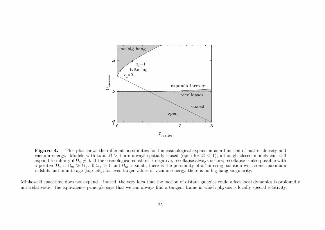
Figure 4. This plot shows the different possibilities for the cosmological expansion as a function of matter density andvacuum energy. Models with total Ω > 1 are always spatially closed (open for Ω < 1), although closed models can stillexpand to infinity if Ωv = 0. If the cosmological constant is negative, recollapse always occurs; recollapse is also possible witha positive Ωv if Ωm � Ωv. If Ωv > 1 and Ωm is small, there is the possibility of a ‘loitering’ solution with some maximumredshift and infinite age (top left); for even larger values of vacuum energy, there is no big bang singularity.

Minkowski spacetime does not expand – indeed, the very idea that the motion of distant galaxies could affect local dynamics is profoundlyanti-relativistic: the equivalence principle says that we can always find a tangent frame in which physics is locally special relativity.

25

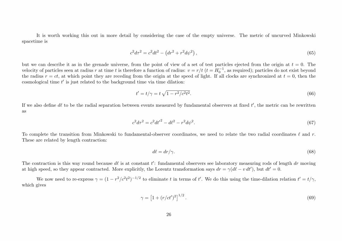
It is worth working this out in more detail by considering the case of the empty universe. The metric of uncurved Minkowskispacetime is

c2dτ2 = c2dt2 − (dr2 + r2dψ2

), (65)

but we can describe it as in the grenade universe, from the point of view of a set of test particles ejected from the origin at t = 0. Thevelocity of particles seen at radius r at time t is therefore a function of radius: v = r/t (t = H−1

0 , as required); particles do not exist beyondthe radius r = ct, at which point they are receding from the origin at the speed of light. If all clocks are synchronized at t = 0, then thecosmological time t′ is just related to the background time via time dilation:

t′ = t/γ = t√1− r2/c2t2. (66)

If we also define d� to be the radial separation between events measured by fundamental observers at fixed t′, the metric can be rewrittenas

c2dτ2 = c2dt′2 − d�2 − r2dψ2. (67)

To complete the transition from Minkowski to fundamental-observer coordinates, we need to relate the two radial coordinates � and r.These are related by length contraction:

d� = dr/γ. (68)

The contraction is this way round because d� is at constant t′: fundamental observers see laboratory measuring rods of length dr movingat high speed, so they appear contracted. More explicitly, the Lorentz transformation says dr = γ(d�− v dt′), but dt′ = 0.

We now need to re-express γ = (1− r2/c2t2)−1/2 to eliminate t in terms of t′. We do this using the time-dilation relation t′ = t/γ,which gives

γ =[1 + (r/ct′)2

]1/2. (69)

26

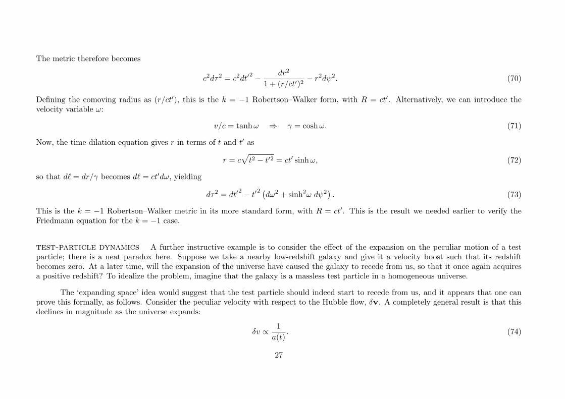
The metric therefore becomes

c2dτ2 = c2dt′2 − dr2

1 + (r/ct′)2− r2dψ2. (70)

Defining the comoving radius as (r/ct′), this is the k = −1 Robertson–Walker form, with R = ct′. Alternatively, we can introduce thevelocity variable ω:

v/c = tanhω ⇒ γ = coshω. (71)

Now, the time-dilation equation gives r in terms of t and t′ as

r = c√t2 − t′2 = ct′ sinhω, (72)

so that d� = dr/γ becomes d� = ct′dω, yielding

dτ2 = dt′2 − t′2 (dω2 + sinh2ω dψ2

). (73)

This is the k = −1 Robertson–Walker metric in its more standard form, with R = ct′. This is the result we needed earlier to verify theFriedmann equation for the k = −1 case.

test-particle dynamics A further instructive example is to consider the effect of the expansion on the peculiar motion of a testparticle; there is a neat paradox here. Suppose we take a nearby low-redshift galaxy and give it a velocity boost such that its redshiftbecomes zero. At a later time, will the expansion of the universe have caused the galaxy to recede from us, so that it once again acquiresa positive redshift? To idealize the problem, imagine that the galaxy is a massless test particle in a homogeneous universe.

The ‘expanding space’ idea would suggest that the test particle should indeed start to recede from us, and it appears that one canprove this formally, as follows. Consider the peculiar velocity with respect to the Hubble flow, δv. A completely general result is that thisdeclines in magnitude as the universe expands:

δv ∝ 1

a(t). (74)

27

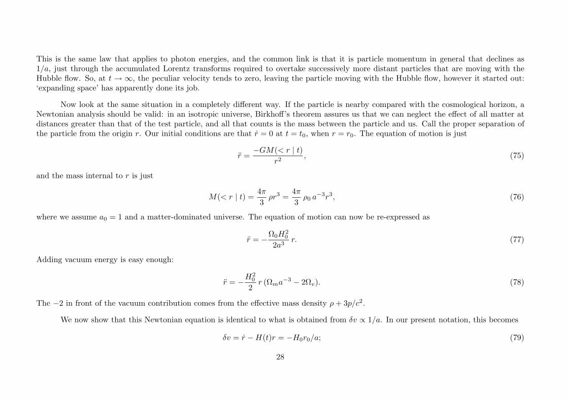
This is the same law that applies to photon energies, and the common link is that it is particle momentum in general that declines as1/a, just through the accumulated Lorentz transforms required to overtake successively more distant particles that are moving with theHubble flow. So, at t → ∞, the peculiar velocity tends to zero, leaving the particle moving with the Hubble flow, however it started out:‘expanding space’ has apparently done its job.

Now look at the same situation in a completely different way. If the particle is nearby compared with the cosmological horizon, aNewtonian analysis should be valid: in an isotropic universe, Birkhoff’s theorem assures us that we can neglect the effect of all matter atdistances greater than that of the test particle, and all that counts is the mass between the particle and us. Call the proper separation ofthe particle from the origin r. Our initial conditions are that r = 0 at t = t0, when r = r0. The equation of motion is just

r =−GM(< r | t)

r2, (75)

and the mass internal to r is just

M(< r | t) = 4π

3ρr3 =

4π

3ρ0 a

−3r3, (76)

where we assume a0 = 1 and a matter-dominated universe. The equation of motion can now be re-expressed as

r = −Ω0H20

2a3r. (77)

Adding vacuum energy is easy enough:

r = −H20

2r (Ωma

−3 − 2Ωv). (78)

The −2 in front of the vacuum contribution comes from the effective mass density ρ+ 3p/c2.

We now show that this Newtonian equation is identical to what is obtained from δv ∝ 1/a. In our present notation, this becomes

δv = r −H(t)r = −H0r0/a; (79)

28

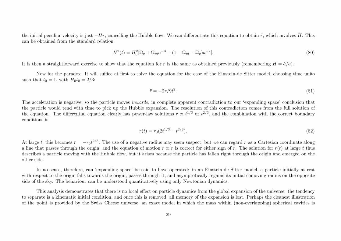
the initial peculiar velocity is just −Hr, cancelling the Hubble flow. We can differentiate this equation to obtain r, which involves H. Thiscan be obtained from the standard relation

H2(t) = H20 [Ωv +Ωma

−3 + (1− Ωm − Ωv)a−2]. (80)

It is then a straightforward exercise to show that the equation for r is the same as obtained previously (remembering H = a/a).

Now for the paradox. It will suffice at first to solve the equation for the case of the Einstein-de Sitter model, choosing time unitssuch that t0 = 1, with H0t0 = 2/3:

r = −2r/9t2. (81)

The acceleration is negative, so the particle moves inwards, in complete apparent contradiction to our ‘expanding space’ conclusion thatthe particle would tend with time to pick up the Hubble expansion. The resolution of this contradiction comes from the full solution ofthe equation. The differential equation clearly has power-law solutions r ∝ t1/3 or t2/3, and the combination with the correct boundaryconditions is

r(t) = r0(2t1/3 − t2/3). (82)

At large t, this becomes r = −r0t2/3. The use of a negative radius may seem suspect, but we can regard r as a Cartesian coordinate alonga line that passes through the origin, and the equation of motion r ∝ r is correct for either sign of r. The solution for r(t) at large t thusdescribes a particle moving with the Hubble flow, but it arises because the particle has fallen right through the origin and emerged on theother side.

In no sense, therefore, can ‘expanding space’ be said to have operated: in an Einstein-de Sitter model, a particle initially at restwith respect to the origin falls towards the origin, passes through it, and asymptotically regains its initial comoving radius on the oppositeside of the sky. The behaviour can be understood quantitatively using only Newtonian dynamics.

This analysis demonstrates that there is no local effect on particle dynamics from the global expansion of the universe: the tendencyto separate is a kinematic initial condition, and once this is removed, all memory of the expansion is lost. Perhaps the cleanest illustrationof the point is provided by the Swiss Cheese universe, an exact model in which the mass within (non-overlapping) spherical cavities is

29

compressed to a black hole. Within the cavity, the metric is exactly Schwarzschild, and the behaviour of the rest of the universe is irrelevant.This avoids the small complication that arises when considering test particles in a homogeneous universe, where we still have to considerthe gravitational effects of the matter between the particles. It should now be clear how to deal with the question, “does the expansion ofthe universe cause the Earth and Moon to separate?”, and that the answer is not the commonly-encountered “it would do, if they weren’theld together by gravity”.

Two further cases are worth considering. In an empty universe, the equation of motion is r = 0, so the particle remains at r = r0,while the universe expands linearly with a ∝ t. In this case, H = 1/t, so that δv = −Hr0, which declines as 1/a, as required. Finally,models with vacuum energy are of more interest. Provided Ωv > Ωm/2, r is initially positive, and the particle does move away from theorigin. This is the criterion for q0 < 0 and an accelerating expansion. In this case, there is a tendency for the particle to expand away fromthe origin, and this is caused by the repulsive effects of vacuum energy. In the limiting case of pure de Sitter space (Ωm = 0, Ωv = 1), theparticle’s trajectory is

r = r0 coshH0(t− t0), (83)

which asymptotically approaches half the r = r0 expH0(t− t0) that would have applied if we had never perturbed the particle in the firstplace. In the case of vacuum-dominated models, then, the repulsive effects of vacuum energy cause all pairs of particles to separate at largetimes, whatever their initial kinematics; this behaviour could perhaps legitimately be called ‘expanding space’. Nevertheless, the effectstems from the clear physical cause of vacuum repulsion, and there is no new physical influence that arises purely from the fact that theuniverse expands. The earlier examples have proved that ‘expanding space’ is in general a dangerously flawed way of thinking about anexpanding universe.

1.9 Observational cosmology

age of the universe Since 1 + z = R0/R(z), we have

dz

dt= −R0

R2

dR

dt= −(1 + z)H(z), (84)

30

so t =∫H(z)−1 dz/(1 + z), where

H2(a) = H20

[Ωv +Ωma

−3 +Ωra−4 − (Ω− 1)a−2

]. (85)

This can’t be done analytically in general, but the following simple approximate formula is accurate to a few % for cases of practical interest:

H0t0 � 2

3(0.7Ωm − 0.3Ωv + 0.3)−0.3. (86)

For a flat universe, the age is H0t0 � (2/3)Ω−0.3m . For many years, estimates of this product were around unity, which is hard to understand

without vacuum energy, unless the density is very low (H0t0 is exactly 1 in the limit of an empty universe). This was one of the firstastronomical motivations for a vacuum-dominated universe.

distance-redshift relation The equation of motion for a photon is Rdr = c dt, so R0dr/dz = (1 + z)c dt/dz, or

R0r =

∫c

H(z)dz. (87)

Remember that non-flat models need the combination R0Sk(r), so one has to divide the above integral by R0 = (c/H0)|Ω− 1|−1/2, applythe Sk function, and then multiply by R0 again. Once more, this process is not analytic in general.

particle horizon If the integral for comoving radius is taken from z = 0 to ∞, we get the full distance a particle can have travelledsince the big bang – the horizon distance. For flat matter-dominated models,

R0rH � 2c

H0Ω−0.4

m . (88)

At high redshift, where H increases, this tends to zero. The onset of radiation domination does not change this: even though the presentlyvisible universe was once very small, it expanded so quickly that causal contact was not easy. The observed large-scale near-homogeneityis therefore something of a puzzle.

31

angular diameters Recall the RW metric:

c2dτ2 = c2dt2 −R2(t)[dr2 + S2

k(r) dψ2]. (89)

The spatial parts of the metric give the proper transverse size of an object seen by us as its comoving size dψ Sk(r) times the scale factorat the time of emission:

d�⊥ = dψ R(z)Sk(r) = dψ R0Sk(r)/(1 + z). (90)

If we know r, we can therefore convert the angle subtended by an object into its physical extent perpendicular to the line of sight.

luminosity and flux density Imagine a source at the centre of a sphere, on which we sit. The photons from the source pass thougha proper surface area 4π[R0Sk(r)]

2. But redshift still affects the flux density in four further ways: (1) photon energies are redshifted, reducingthe flux density by a factor 1+ z; (2) photon arrival rates are time dilated, reducing the flux density by a further factor 1+ z; (3) opposingthis, the bandwidth dν is reduced by a factor 1+z, which increases the energy flux per unit bandwidth by one power of 1+z; (4) finally, theobserved photons at frequency ν0 were emitted at frequency [1 + z]× ν0. Overall, the flux density is the luminosity at frequency [1 + z]ν0,divided by the total area, divided by 1 + z:

Sν(ν0) =Lν([1 + z]ν0)

4πR20S

2k(r)(1 + z)

=Lν(ν0)

4πR20S

2k(r)(1 + z)1+α

, (91)

where the second expression assumes a power-law spectrum L ∝ ν−α.

surface brightness The flux density is the product of the specific intensity Iν and the solid angle subtended by the source:Sν = Iν dΩ. Combining the angular size and flux-density relations gives a relation that is independent of cosmology:

Iν(ν0) =Bν([1 + z]ν0)

(1 + z)3, (92)

32

where Bν is surface brightness (luminosity emitted into unit solid angle per unit area of source). This (1+ z)3 dimming makes it hardto detect extended objects at very high redshift. The factor becomes (1 + z)4 if we integrate over frequency to get a bolometric quantity.

effective distances The angle and flux relations can be made to look Euclidean:

angular− diameter distance : DA = (1 + z)−1R0Sk(r)

luminosity distance : DL = (1 + z) R0Sk(r).(93)

Some example distance-redshift relations are shown in figure 5. Notice how a high matter density tends to make high-redshift objectsbrighter: stronger deceleration means they are closer for a given redshift.

Recall that the comoving distance approaches that of the particle horizon as z →∞. Here, there is a substantial dependence on thematter density, but in a way that differs depending on whether or not there is vacuum energy:

R0Sk(r) = (2c/H0)Ω−1m (open); (or) (2c/H0)Ω

−0.4m (flat). (94)

The first relation is exact; the second is an accurate approximation.

1.10 Absolute magnitude and K-correction

Absolute magnitude is defined as the apparent magnitude that would be observed if the source lay at a distance of 10 pc; it is just a measureof luminosity. Absolute magnitudes in cosmology are affected by a shift of the spectrum in frequency; the K-correction accounts for thiseffect, giving the difference between the observed dimming with redshift for a fixed observing waveband, and that expected on bolometricgrounds:

m =M + 5 log10

(DL

10 pc

)+K(z), (95)

33

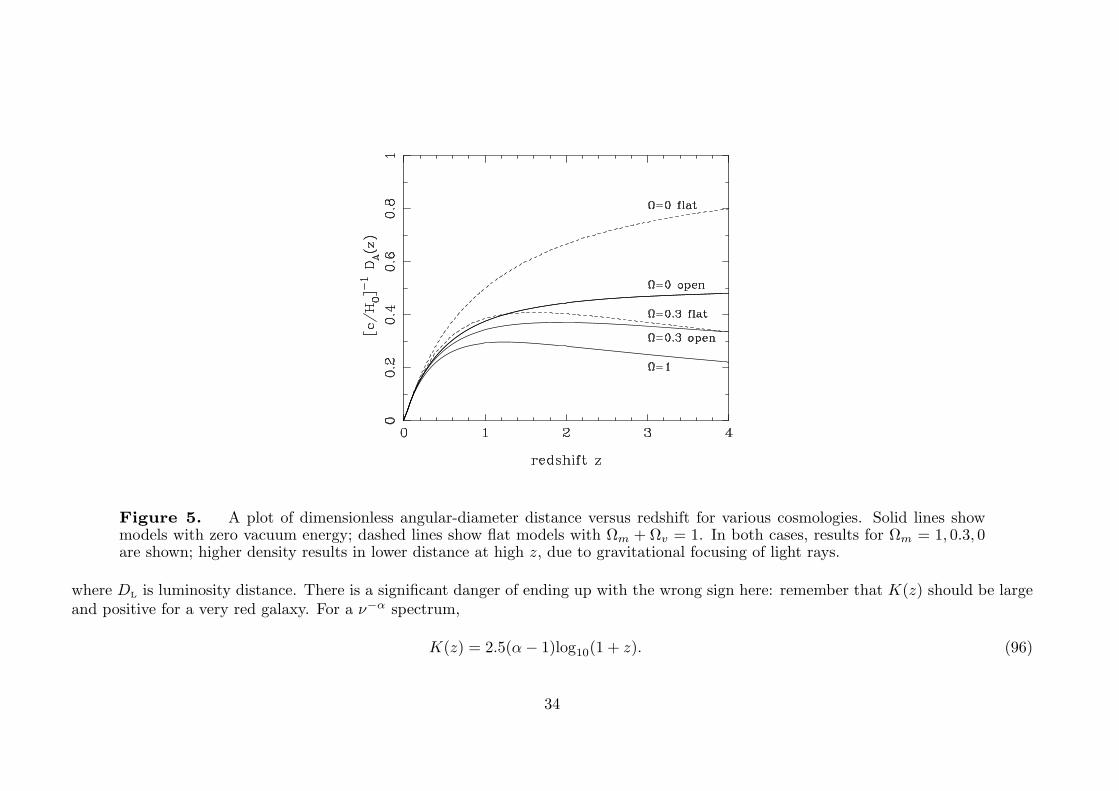
Figure 5. A plot of dimensionless angular-diameter distance versus redshift for various cosmologies. Solid lines showmodels with zero vacuum energy; dashed lines show flat models with Ωm + Ωv = 1. In both cases, results for Ωm = 1, 0.3, 0are shown; higher density results in lower distance at high z, due to gravitational focusing of light rays.

where DL is luminosity distance. There is a significant danger of ending up with the wrong sign here: remember that K(z) should be largeand positive for a very red galaxy. For a ν−α spectrum,

K(z) = 2.5(α− 1)log10(1 + z). (96)

34

1.11 Counts and luminosity functions

We now have all the tools needed to understand how astronomical observations sample the population of objects in the universe. Historically,this began with almost no information on redshifts (which are still hard to obtain for the faintest objects). Nevertheless, there is usefulinformation just in the number counts.

euclidean counts The number–flux relation assumes an important form if space is Euclidean. Consider first a universe populatedwith sources that all have the same luminosity, with number density n. The flux density is now just the normal inverse-square lawS = L/(4πD2), so the distance to a given object is proportional to (L/S)1/2. The number of objects brighter than S is just n times thevolume of space within which they can be seen:

N(> S) = nV (S) = n(A/3)(L/4πS)3/2 ∝ S−3/2, (97)

where A is the solid angle of the survey. This Euclidean source count is the baseline for all realistic surveys, and shows us that faintsources are likely to heavily outnumber bright ones. It obviously remains true if we now add in a more realistic population of sources witha wide range of luminosities. The relation is one form of Olbers’ paradox: integration over S implies a divergent sky brightness:

I =

∫S dN(S)/A. (98)

Since the universe does not contain an infinite energy density, it is clear that relativistic effects in the distance–redshift and volume–redshiftrelations must cause the true counts to lie below the Euclidean prediction.

luminosity functions The evolution of the properties of a population of cosmological sources can be described via the luminosityfunction φ(L), which is the comoving number density of objects in some range of luminosity. Generally, the simplest results arise if we takeφ to be the comoving density per interval of lnL:

dN = φ(L, z) d lnL dV (z). (99)

35

It is often convenient to describe the results analytically e.g. via a Schechter function fit at each redshift

dφ = φ∗(L/L∗)α exp(−L/L∗) dL/L∗. (100)

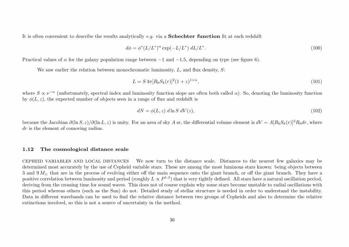
Practical values of α for the galaxy population range between −1 and −1.5, depending on type (see figure 6).We saw earlier the relation between monochromatic luminosity, L, and flux density, S:

L = S 4π[R0Sk(r)]2(1 + z)1+α, (101)

where S ∝ ν−α (unfortunately, spectral index and luminosity function slope are often both called α). So, denoting the luminosity functionby φ(L, z), the expected number of objects seen in a range of flux and redshift is

dN = φ(L, z) d lnS dV (z), (102)

because the Jacobian ∂(lnS, z)/∂(lnL, z) is unity. For an area of sky A sr, the differential volume element is dV = A[R0Sk(r)]2R0dr, where

dr is the element of comoving radius.

1.12 The cosmological distance scale

cepheid variables and local distances We now turn to the distance scale. Distances to the nearest few galaxies may bedetermined most accurately by the use of Cepheid variable stars. These are among the most luminous stars known: being objects between3 and 9M� that are in the process of evolving either off the main sequence onto the giant branch, or off the giant branch. They have apositive correlation between luminosity and period (roughly L ∝ P 1.3) that is very tightly defined. All stars have a natural oscillation period,deriving from the crossing time for sound waves. This does not of course explain why some stars become unstable to radial oscillations withthis period whereas others (such as the Sun) do not. Detailed study of stellar structure is needed in order to understand the instability.Data in different wavebands can be used to find the relative distance between two groups of Cepheids and also to determine the relativeextinctions involved, so this is not a source of uncertainty in the method.

36

Figure 6. The galaxy luminosity function, with the population dissected into different types. At the top, we gave galaxieswith old stellar populations (ellipticals); at the bottom, we move to galaxies dominated by younger stars (extreme spiral andirregular galaxies). The latter are systematically less luminous than the former (and less massive). In all cases, a Schechterfunction (power-law times exponential cutoff) gives a good fit.

37

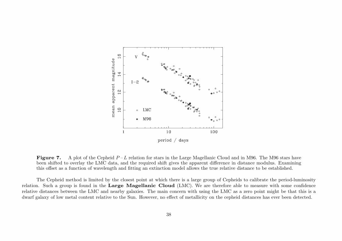
Figure 7. A plot of the Cepheid P –L relation for stars in the Large Magellanic Cloud and in M96. The M96 stars havebeen shifted to overlay the LMC data, and the required shift gives the apparent difference in distance modulus. Examiningthis offset as a function of wavelength and fitting an extinction model allows the true relative distance to be established.

The Cepheid method is limited by the closest point at which there is a large group of Cepheids to calibrate the period-luminosityrelation. Such a group is found in the Large Magellanic Cloud (LMC). We are therefore able to measure with some confidencerelative distances between the LMC and nearby galaxies. The main concern with using the LMC as a zero point might be that this is adwarf galaxy of low metal content relative to the Sun. However, no effect of metallicity on the cepheid distances has ever been detected.

38

This leaves the absolute distance to the LMC as one of the key numbers in cosmology, and we have a reasonably good idea what itis:

DLMC = 51 kpc ± 6%. (103)

This number has been established over the years by a number of methods. The simplest is to calibrate the luminosities of a few morenearby cepheids. This is done via main-sequence fitting (finding the offset in apparent magnitude at a given colour) of the HR diagramsof the star clusters that host Cepheids. For the most nearby star clusters, distances can be obtained via trigonometric parallax or relatedmethods (the astrometric HIPPARCOS satellite has had a big impact here). A much more direct alternative came from observationsof SN1987A: a supernova that took place in the LMC itself. This was observed to produce a ring of emission that was elliptical tohigh precision – and therefore almost certainly a circular ring seen inclined. Different parts of the ring were observed being illuminated atdifferent times owing to finite light travel-time effects. Knowing the inclination, plus the observed angular size of the ring, the distance tothe supernova follows. It agrees very well with the traditional figure.

1.13 Larger distances: the supernova Hubble diagram

Cepheid distances can thus be found for the more nearby galaxies. The Hubble Space Telescope has allowed this to be done for afew dozen galaxies out to distances of 10 to 20 Mpc. Unfortunately, this is not really far enough. At 10 Mpc, the recessional velocity is1000h km s−1, but peculiar velocities can reach 600 km s−1. In order to determine H0 accurately, we need to attain recessional velocities of> 10, 000 km s−1.

This requires brighter objects than Cepheids, and traditional work concentrated on whole-galaxy luminosity indicators. These arevariants of the Tully-Fisher relation, which says that the luminosity of a spiral galaxy scales with its rotational velocity roughly asL ∝ V 3. This is reminiscent of V 2 = GM/r, but obviously raises questions about M/L ratios and sizes of galaxies. In any case, suchmethods are of limited accuracy, predicting L to about 40%, and hence giving relative distances to about 20% precision. The great discoveryof the 1990s was that supernovae make much more accurate standard candles.

39

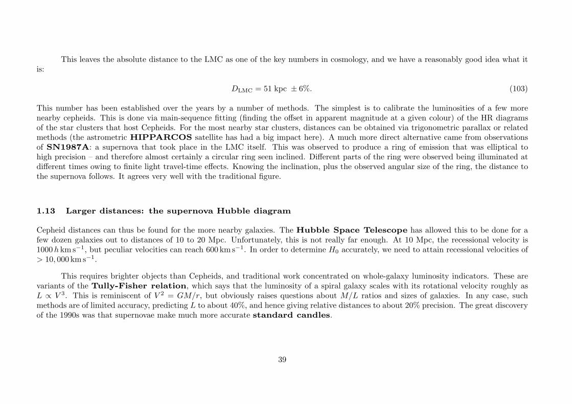
Figure 8. The type Ia supernova Hubble diagram. Using a measure of characteristic time as well as peak luminosityfor the light curve, relative distances to individual SNe can be measured to 6% rms. Setting the absolute distance scale (DL

is luminosity distance) using local SNe in galaxies with Cepheid distances shows that the large-scale Hubble flow is indeedlinear and uniform, and gives an estimate of H0 = 72± 8 km s−1Mpc−1.

Supernovae come in two-and-a-bit varieties, SNe Ia, Ib and II, distinguished according to whether or not they display absorptionand emission lines of hydrogen. The SNe II do show hydrogen; they are associated with massive stars at the endpoint of their evolution,and are rather heterogeneous in their behaviour. The former, especially SNe Ia, are much more homogeneous in their properties, and canbe used as standard candles. There is a characteristic rise to maximum, followed by a symmetric fall over roughly 30 days, after which thelight decay becomes less rapid. Type Ib SNe are a complication to the scheme; they do not have the characteristic light curve, and alsolack hydrogen lines.

40

The simplest use of these supernovae was to note that they empirically have a very small dispersion in luminosity at maximum light(<∼ 0.3 magnitudes). However, one might legitimately ask why SNe Ia should be standard candles. After all, presumably the progenitorstars vary in mass, and this should affect the energy output. A more satisfactory treatment of the supernovae distance scale takes thispossibility into account by measuring both the height of the light curve (apparent luminosity at maximum light) and the width (timetaken to reach maximum light, or other equivalent measures). For SNe where relative distances are known by some other method, theseparameters are seen to correlate: the maximum output of SNe scales as roughly the 1.7 power of the characteristic timescale. The physicalinterpretation of this relation is that both the measured parameters depend on mass: a more massive star has more fuel and so generatesa more energetic explosion, but the resulting fireball has to expand for longer in order for its optical depth to reach unity, allowing thephotons to escape.

It is therefore possible to turn SNe Ia into genuine standard candles, and the accuracy is astonishingly good: a corrected dispersion of0.12 magnitudes, implying that relative distances to a single SN can be measured to 6% precision. The SN Hubble diagram is impressivelylinear (figure 8), and allows a very precise estimate of H0, based on the HST Cepheid distances:

H0 = 72± 8 km s−1Mpc−1. (104)

The uncertainty on this now comes largely from how accurately we know the distance to the LMC.

Values for t0 in the range 12 – 16 Gyr are a reasonable summary of the present estimates from stellar evolution. If the globular-clusterages are not trusted, however, nuclear decay ages do not compel us to believe that the universe is any older than 9 Gyr. If we take aconservative range from above of 0.6 < h < 0.84, that allows an extreme range of

0.55 < H0t0 � 23

(0.7Ωm + 0.3− 0.3Ωv

)−0.3< 1.37, (105)

with a best guess of H0t0 � 0.96, for h = 0.72 and t0 = 13 Gyr. If Ωm > 0.1 is accepted as a hard lower bound, then vacuum energy isrequired on the basis of this formula if H0t0 > 0.90. The Einstein–de Sitter model requires H0t0 = 2/3, and is very hard to reconcile withthe data. The high apparent value of H0t0 was historically one of the first indication that vacuum energy might be required in cosmology.

41

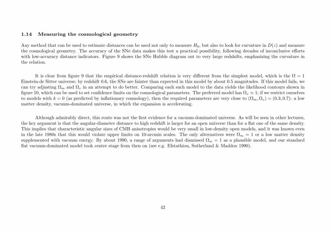
1.14 Measuring the cosmological geometry

Any method that can be used to estimate distances can be used not only to measure H0, but also to look for curvature in D(z) and measurethe cosmological geometry. The accuracy of the SNe data makes this test a practical possibility, following decades of inconclusive effortswith low-accuracy distance indicators. Figure 9 shows the SNe Hubble diagram out to very large redshifts, emphasizing the curvature inthe relation.

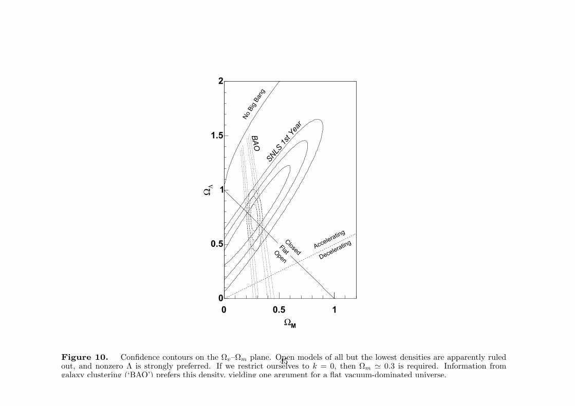
It is clear from figure 9 that the empirical distance-redshift relation is very different from the simplest model, which is the Ω = 1Einstein-de Sitter universe; by redshift 0.6, the SNe are fainter than expected in this model by about 0.5 magnitudes. If this model fails, wecan try adjusting Ωm and Ωv in an attempt to do better. Comparing each such model to the data yields the likelihood contours shown infigure 10, which can be used to set confidence limits on the cosmological parameters. The preferred model has Ωv � 1; if we restrict ourselvesto models with k = 0 (as predicted by inflationary cosmology), then the required parameters are very close to (Ωm,Ωv) = (0.3, 0.7): a lowmatter density, vacuum-dominated universe, in which the expansion is accelerating.

Although admirably direct, this route was not the first evidence for a vacuum-dominated universe. As will be seen in other lectures,the key argument is that the angular-diameter distance to high redshift is larger for an open universe than for a flat one of the same density.This implies that characteristic angular sizes of CMB anisotropies would be very small in low-density open models, and it was known evenin the late 1980s that this would violate upper limits on 10-arcmin scales. The only alternatives were Ωm = 1 or a low matter densitysupplemented with vacuum energy. By about 1990, a range of arguments had dismissed Ωm = 1 as a plausible model, and our standardflat vacuum-dominated model took centre stage from then on (see e.g. Efstathiou, Sutherland & Maddox 1990).

42

SN Redshift0.2 0.4 0.6 0.8 1

Bμ

34

36

38

40

42

44

)=(0.26,0.74)ΛΩ,mΩ(

)=(1.00,0.00)ΛΩ,mΩ(

SNLS 1st Year

SN Redshift0.2 0.4 0.6 0.8 1

) 0 H

-1 c L

( d

10 -

5 lo

gBμ

-1

-0.5

0

0.5

1

Figure 9. The Hubble diagram. The lower panel shows the data divided by a default model (flat Ωm = 0.26). The resultslie clearly match this model, very precisely. The lowest line is the Einstein-de Sitter model, which is in gross disagreementwith observation. 43

2 The perturbed universe

All discussion so far has applied to homogeneous models, but of course the real universe contains structure. The study of this structure viagalaxy clustering and the CMB is the subject of separate courses here, but it may help to summarise some aspects of this in a way thatshould be complementary and fill in relevant background.

quantifying inhomogeneity The first issue we have to deal with is how to quantify departures from uniform density. Frequently,an intuitive Newtonian approach can be used, and we will adopt this wherever possible. But we should begin with a quick overview of therelativistic approach to this problem, to emphasise some of the big issues that are ignored in the Newtonian method.

Because relativistic physics equations are written in a covariant form in which all quantities are independent of coordinates, relativitydoes not distinguish between active changes of coordinate (e.g. a Lorentz boost) or passive changes (a mathematical change of variable,normally termed a gauge transformation). This generality is a problem, as we can see by asking how some scalar quantity S (which mightbe density, temperature etc.) changes under a gauge transformation xμ → x′μ = xμ+εμ. A gauge transformation induces the usual Lorentztransformation coefficients dx′μ/dxν (which have no effect on a scalar), but also involves a translation that relabels spacetime points. Wetherefore have S′(xμ + εμ) = S(xμ), or

S′(xμ) = S(xμ)− εα∂S/∂xα. (106)

Consider applying this to the case of a uniform universe; here ρ only depends on time, so that

ρ′ = ρ− ε0ρ. (107)

An effective density perturbation is thus produced by a local alteration in the time coordinate: when we look at a universe with a fluctuatingdensity, should we really think of a uniform model in which time is wrinkled? This ambiguity may seem absurd, and in the laboratoryit could be resolved empirically by constructing the coordinate system directly – in principle by using light signals. This shows thatthe cosmological horizon plays an important role in this topic: perturbations with wavelength λ <

∼ ct inhabit a regime in which gauge

44

MΩ0 0.5 1

ΛΩ

0

0.5

1

1.5

2

SNLS 1s

t Yea

r

BAO

ClosedFlatOpen

Accelerating

DeceleratingNo

Big

Bang

Figure 10. Confidence contours on the Ωv–Ωm plane. Open models of all but the lowest densities are apparently ruledout, and nonzero Λ is strongly preferred. If we restrict ourselves to k = 0, then Ωm � 0.3 is required. Information fromgalaxy clustering (‘BAO’) prefers this density, yielding one argument for a flat vacuum-dominated universe.

45

ambiguities can be resolved directly via common sense. The real difficulties lie in the super-horizon modes with λ >∼ ct. Within inflationarymodels, however, these difficulties can be overcome, since the true horizon is � ct.

The most direct general way of solving these difficulties is to construct perturbation variables that are explicitly independent ofgauge. A comprehensive technical discussion of this method is given in chapter 7 of Mukhanov’s book, and we summarize the essentialelements here, largely without proof. First, we need to devise a notation that will classify the possible perturbations. Since the metricis symmetric, there are 10 independent degrees of freedom in gμν ; a convenient scheme that captures these possibilities is to write thecosmological metric as

dτ2 = a2(η){(1 + 2φ)dη2 + 2widη dx

i − [(1− 2ψ)γij + 2hij ] dxi dxj

}. (108)

In this equation, η is conformal time,

dη = dt/a(t), (109)

and γij is the comoving spatial part of the Robertson-Walker metric.

The total number of degrees of freedom here is apparently 2 (scalar fields φ and ψ) + 3 (3-vector field w) + 6 (symmetric 3-tensorhij) = 11. To get the right number, the tensor hij is required to be traceless: γ

ijhij = 0. The perturbations can be split into three classes:scalar perturbations, which are described by scalar functions of spacetime coordinate, and which correspond to growing densityperturbations; vector perturbations, which correspond to vorticity perturbations, and tensor perturbations, which correspondto gravitational waves. Here, we shall concentrate mainly on scalar perturbations.

Since vectors and tensors can be generated from derivatives of a scalar function, the most general scalar perturbation actually makescontributions to all the gμν components in the above expansion:

δgμν = a2

(2φ −B,i

−B,i 2[ψδij − E,ij ]

), (110)

46

where four scalar functions φ, ψ, E and B are involved. It turns out that this situation can be simplified by defining variables that areunchanged by a gauge transformation:

Φ ≡ φ+1

a[(B − E′)a]′

Ψ ≡ ψ − a′

a(B − E′),

(111)

where primes denote derivatives with respect to conformal time.

These gauge-invariant ‘potentials’ have a fairly direct physical interpretation, since they are closely related to the Newtonian potential.The easiest way to evaluate the gauge-invariant fields is to make a specific gauge choice and work with the longitudinal gauge in whichE and B vanish, so that Φ = φ and Ψ = ψ. A second key result is that inserting the longitudinal metric into the Einstein equations showsthat φ and ψ are identical in the case of fluid-like perturbations where off-diagonal elements of the energy–momentum tensor vanish. Inthis case, the longitudinal gauge becomes identical to the Newtonian gauge, in which perturbations are described by a single scalarfield, which is the gravitational potential. The conclusion is thus that the gravitational potential can for many purposes give an effectivelygauge-invariant measure of cosmological perturbations, and this provides a sounder justification for the Newtonian approach that we nowadopt. The Newtonian-gauge metric therefore looks like this:

dτ2 = (1 + 2Φ)dt2 − (1− 2Φ)γij dxi dxj , (112)

and this should be quite familiar. If we consider small scales, so that the spatial metric γij becomes that of flat space, then this formmatches, for example, the Schwarzschild metric with Φ = −GM/r, in the limit Φ/c2 � 1.

Informally, the potential Φ is a measure of space-time curvature which solves the gauge issue and has meaning on super-horizonscales. A key property, which is perhaps intuitively reasonable, is that Φ is constant in time for perturbations with wavelengths much largerthan the horizon. Conversely, interesting effects can happen inside the horizon, which imprints characteristic scale-dependent features on thecosmological inhomogeneities. A full justification of the constancy of Φ using a complete relativistic treatment would take too much space,and we will generally discuss perturbations using a Newtonian approach. This does yield the correct conclusion regarding the constancy ofΦ, but we should be clear that this is at best a consistency check, since we will use a treatment of gravity that is restricted to static fields.

47

fluctuation power spectra From the Newtonian point of view, potential fluctuations are directly related to those in density viaPoisson’s equation:

∇2Φ/a2 = 4πG(1 + 3w) ρ δ, (113)

where we have defined a dimensionless fluctuation amplitude

δ ≡ ρ− ρρ

. (114)

the factor of a2 is there so we can use comoving length units in ∇2 and the factor (1 + 3w) accounts for the relativistic active mass densityρ+ 3p.

We are very often interested in asking how these fluctuations depend on scale, which amounts to making a Fourier expansion:

δ(x) =∑

δke−ik·x, (115)

where k is the comoving wavevector. What are the allowed modes? If the field were periodic within some box of side L, we would have theusual harmonic boundary conditions

kx = n2π

L, n = 1, 2 · · · , (116)

and the inverse Fourier relation would be

δk(k) =

(1

L

)3 ∫δ(x) exp

(ik · x)

d3x. (117)

Working in Fourier space in this way is powerful because it immediately gives a way of solving Poisson’s equation and relating fluctuationsin density and potential. For a single mode, ∇2 → −k2, and so

Φk = −4πG(1 + 3w)a2 ρ δk/k2. (118)

48

The fluctuating density field can be described by its statistical properties. The mean is zero by construction; the variance is obtainedby taking the volume average of δ2:

〈δ2〉 =∑

|δk|2. (119)

To see this result, write the lhs instead as 〈δδ∗〉 (makes no difference for a real field), and appreciate that all cross terms integrate to zerovia the boundary conditions. For obvious reasons, the quantity

P (k) ≡ |δk|2 (120)

is called the power spectrum. Note that, in an isotropic universe, we assume that P will be independent of direction of the wavevectorin the limit of a large box: the fluctuating density field is statistically isotropic. In applying this apparatus, we would not want the(arbitrary) box size to appear. This happens naturally: as the box becomes big, the modes are finely spaced and a sum over modes isreplaced by an integral over k space times the usual density of states, (L/2π)3:

〈δ2〉 =∑

|δk|2 → L3

(2π)3

∫P (k) d3k =

∫Δ2(k) d ln k. (121)

In the last step, we have defined the combination

Δ2(k) ≡ L3

(2π)34πk3 P (k), (122)

which absorbs the box size into the definition of a dimensionless power spectrum, which gives the contribution to the variance from eachlogarithmic range of wavenumber (or wavelength).

49

2.1 Growth of linear perturbations

We have decided that perturbations will in most cases effectively be described by the Newtonian potential, Φ. Now we need to developan equation of motion for Φ, or equivalently for the density fluctuation ρ ≡ (1 + δ)ρ. In the Newtonian approach, we treat dynamics ofcosmological matter exactly as we would in the laboratory, by finding the equations of motion induced by either pressure or gravity. Webegin by casting the problem in comoving units:

x(t) = a(t)r(t)

δv(t) = a(t)u(t),(123)

so that x has units of proper length, i.e. it is an Eulerian coordinate. First note that the comoving peculiar velocity u is just thetime derivative of the comoving coordinate r:

x = ar+ ar = Hx+ ar, (124)

where the rhs must be equal to the Hubble flow Hx, plus the peculiar velocity δv = au.

The equation of motion follows from writing the Eulerian equation of motion as x = g0 + g, where g = −∇∇∇∇∇∇∇∇∇∇∇∇∇Φ/a is the peculiaracceleration, and g0 is the acceleration that acts on a particle in a homogeneous universe (neglecting pressure forces to start with, forsimplicity). Differentiating x = ar twice gives

x = au+ 2au+a

ax = g0 + g. (125)

The unperturbed equation corresponds to zero peculiar velocity and zero peculiar acceleration: (a/a)x = g0; subtracting this gives theperturbed equation of motion

u+ 2(a/a)u = g/a. (126)

This equation of motion for the peculiar velocity shows that u is affected by gravitational acceleration and by the Hubble drag term,2(a/a)u. This arises because the peculiar velocity falls with time as a particle attempts to catch up with successively more distant (and

50

therefore more rapidly receding) neighbours. In the absence of gravity, we get δv ∝ 1/a: momentum redshifts away, just as with photonenergy.

The peculiar velocity is directly related to the evolution of the density field, through conservation of mass. This is expressed via thecontinuity equation, which takes the form

d

dtρ0(1 + δ) = −ρ0(1 + δ)∇∇∇∇∇∇∇∇∇∇∇∇∇ · u. (127)

As usual, spatial derivatives are with respect to comoving coordinates:

∇∇∇∇∇∇∇∇∇∇∇∇∇ ≡ a∇∇∇∇∇∇∇∇∇∇∇∇∇proper, (128)

and the time derivative is a convective one:

d

dt=

∂

∂t+ u · ∇∇∇∇∇∇∇∇∇∇∇∇∇, (129)

i.e. the time derivative measured by an observer who follows a particle’s trajectory. Finally, when using a comoving frame, the backgrounddensity ρ0 is unaffected by d/dt, and so the full continuity equation can be written as

d

dtδ = −(1 + δ)∇∇∇∇∇∇∇∇∇∇∇∇∇ · u. (130)

linear approximation The equation for δ is not linear in the perturbations δ and u. To cure this, we restrict ourselves to the caseδ � 1 and linearize the equation, neglecting second-order terms like δ × u, which removes the distinction between convective and partialtime derivatives. The linearized equations for conservation of momentum and matter as experienced by fundamental observers moving withthe Hubble flow are then:

u+ 2a

au =

g

a

δ = −∇∇∇∇∇∇∇∇∇∇∇∇∇ · u,(131)

51

where the peculiar gravitational acceleration −∇∇∇∇∇∇∇∇∇∇∇∇∇Φ/a is denoted by g.

The solutions of these equations can be decomposed into modes either parallel to g or independent of g (these are the homogeneousand inhomogeneous solutions to the equation of motion). The homogeneous case corresponds to no peculiar gravity – i.e. zero densityperturbation. This is consistent with the linearized continuity equation, ∇∇∇∇∇∇∇∇∇∇∇∇∇ · u = −δ, which says that it is possible to have vorticitymodes with ∇∇∇∇∇∇∇∇∇∇∇∇∇ · u = 0 for which δ vanishes, so there is no growth of structure in this case. The proper velocities of these vorticity modesdecay as v = au ∝ a−1, as with the kinematic analysis for a single particle.

growing mode For the growing mode, it is most convenient to eliminate u by taking the divergence of the equation of motion for u,and the time derivative of the continuity equation. This requires a knowledge of∇∇∇∇∇∇∇∇∇∇∇∇∇·g, which comes via Poisson’s equation: ∇∇∇∇∇∇∇∇∇∇∇∇∇ · g = 4πGaρ0δ.The resulting 2nd-order equation for δ is

δ + 2a

aδ = 4πGρ0 δ. (132)

This is easily solved for the Ωm = 1 case, where 4πGρ0 = 3H2/2 = 2/3t2, and a power-law solution works:

δ(t) ∝ t2/3 or t−1. (133)

The first solution, with δ(t) ∝ a(t) is the growing mode, corresponding to the gravitational instability of density perturbations. Given somesmall initial seed fluctuations, this is the simplest way of creating a universe with any desired degree of inhomogeneity.

One further way of stating this result is that gravitational potential perturbations are independent of time (at least while Ω = 1).Poisson’s equation tells us that −k2Φ/a2 ∝ ρ δ; since ρ ∝ a−3 for matter domination or a−4 for radiation, that gives Φ ∝ δ/a or δ/a2

respectively, so that Φ is independent of a in either case. In other words, the metric fluctuations resulting from potential perturbations arefrozen, at least for perturbations with wavelengths greater than the horizon size.

meszaros effect What about the case of collisionless matter in a radiation background? The fluid treatment is not appropriatehere, since the two species of particles can interpenetrate. A particularly interesting limit is for perturbations well inside the horizon: the

52

radiation can then be treated as a smooth, unclustered background that affects only the overall expansion rate. This is analogous to theeffect of Λ, but an analytical solution does exist in this case. The perturbation equation is as before

δ + 2a

aδ = 4πGρmδ, (134)

but now H2 = 8πG(ρm + ρr)/3. If we change variable to y ≡ ρm/ρr = a/aeq, and use the Friedmann equation, then the growth equationbecomes

δ′′ +2 + 3y

2y(1 + y)δ′ − 3

2y(1 + y)δ = 0 (135)

(for zero curvature, as appropriate for early times). It may be seen by inspection that a growing solution exists with δ′′ = 0:

δ ∝ y + 2/3. (136)

It is also possible to derive the decaying mode. This is simple in the radiation-dominated case (y � 1): δ ∝ − ln y is easily seen to be anapproximate solution in this limit.

What this says is that, at early times, the dominant energy of radiation drives the universe to expand so fast that the matter hasno time to respond, and δ is frozen at a constant value. At late times, the radiation becomes negligible, and the growth increases smoothlyto the Einstein–de Sitter δ ∝ a behaviour (Meszaros 1974). The overall behaviour is therefore reminiscent to the effects of pressure on acoupled fluid, where growth is suppressed below the Jeans scale. However, the two phenomena are really quite different. In the fluid case,the radiation pressure prevents the perturbations from collapsing further; in the collisionless case, the photons have free-streamed away, andthe matter perturbation fails to collapse only because radiation domination ensures that the universe expands too quickly for the matterto have time to self-gravitate.

This effect is critical in shaping the late-time power spectrum. For scales greater than the horizon, perturbations in matter andradiation can grow together, so fluctuations at early times grow at the same rate, independent of wavenumber. But this growth ceasesonce the perturbations ‘enter the horizon’ – i.e. when the horizon grows sufficiently to exceed the perturbation wavelength. At this point,growth ceases, so the universe preserves a ‘snapshot’ of the amplitude of the mode at horizon crossing. For a scale-invariant spectrum, thisimplies a dimensionless power δ2(k) � δ2

Hon small scales, breaking to the initial δ2(k) ∝ k4 on large scales. Observing this break and using

it to measure the density of the universe has been one of the great success stories in recent cosmological research.

53

2.2 Nonlinear structure formation

The equations of motion are nonlinear, and we have only solved them in the limit of linear perturbations. We now discuss evolution beyondthe linear regime, first considering the full numerical solution of the equations of motion, and then a key analytic approximation by whichthe ‘exact’ results can be understood.

n-body models The exact evolution of the density field is usually performed by means of an N-body simulation, in which thedensity field is represented by the sum of a set of fictitious discrete particles. We need to solve the equations of motion for each particle, asit moves in the gravitational field due to all the other particles. Using comoving units for length and velocity (v = au), we have previouslyseen the equation of motion

d

dtu = −2 a

au− 1

a2∇∇∇∇∇∇∇∇∇∇∇∇∇Φ, (137)

where Φ is the Newtonian gravitational potential due to density perturbations. The time derivative is already in the required form of theconvective time derivative observed by a particle, rather than the partial ∂/∂t.

In outline, this is straightforward to solve, given some initial positions and velocities. Defining some timestep dt, particles are movedaccording to dx = u dt, and their velocities updated according to du = u dt, with u given by the equation of motion (in practice, moresophisticated time integration schemes are used). The hard part is finding the gravitational force, since this involves summation over (N−1)other particles each time we need a force for one particle. All the craft in the field involves finding clever ways in which all the forces can beevaluated in less than the raw O(N2) computations per timestep. We will have to omit the details of this, unfortunately, but one obviousway of proceeding is to solve Poisson’s equation on a mesh using a Fast Fourier Transform. This can convert the O(N2) time scaling toO(N lnN), which is a qualitative difference given that N can be as large as 1010.

Computing lives by the ‘garbage in, garbage out’ rule, so how are the initial conditions in the simulation set? This can be understoodby thinking of density fluctuations in Lagrangian terms (also known as the Zeldovich approximation). The proper coordinate ofa given particle can be written as

x(t) = a(t) (q+ f (q, t)) , (138)

54

where q is the usual comoving position, and the displacement field f (q, t) tends to zero at t = 0. The comoving peculiar velocity isjust the time derivative of this displacement:

u =∂f

∂t(139)

(partial time derivative because each particle is labelled by an unchanging value of q – this is what is meant by a Lagrangian coordinate).

By conservation of particles, the density at a given time is just the Jacobian determinant between q and x:

ρ / ρ =

∣∣∣∣ ∂q

∂x/a

∣∣∣∣ . (140)

When the displacement is small, this is just

ρ / ρ = 1−∇∇∇∇∇∇∇∇∇∇∇∇∇ · f (q, t), (141)

so the linear density perturbation δ is just (minus) the divergence of the displacement field. All this can be handled quite simply if wedefine a displacement potential:

f = −∇∇∇∇∇∇∇∇∇∇∇∇∇ψ(q), (142)

from which we have δ = ∇2ψ in the linear regime. The displacement potential ψ is therefore proportional to the gravitational potential, Φ.These equations are easily manipulated in Fourier space: given the amplitudes of the Fourier modes, δk, we can obtain the potential

ψk = −δk/k2, (143)

and hence the displacement and velocity

fk = ikψk

uk = ik ψk.(144)

55

Thus, given the density power spectrum to specify |δk| and the assumption of random phases, we can set up a field of consistent smalldisplacements and consistent velocities. These are applied to a uniform particle ‘load’, and then integrated forward into the nonlinearregime.

the spherical model N -body models can yield evolved density fields that are nearly exact solutions to the equations of motion,but working out what the results mean is then more a question of data analysis than of deep insight. Where possible, it is important tohave analytic models that guide the interpretation of the numerical results. The most important model of this sort is the spherical densityperturbation, which can be analysed immediately using the tools developed for the Friedmann models, since Birkhoff’s theorem tells usthat such a perturbation behaves in exactly the same way as part of a closed universe. The equations of motion are the same as for thescale factor, and we can therefore write down the cycloid solution immediately. For a matter-dominated universe, the relation betweenthe proper radius of the sphere and time is

r = A(1− cos θ)

t = B(θ − sin θ).(145)

It is easy to eliminate θ to obtain r = −GM/r2, and the relation A3 = GMB2 (use e.g. r = (dr/dθ)/((dt/dθ), which givesr = [A/B] sin θ/[1− cos θ]). Expanding these relations up to order θ5 gives r(t) for small t:

r � A

2

(6t

B

)2/3[1− 1

20

(6t

B

)2/3], (146)

and we can identify the density perturbation within the sphere:

δ � 3

20

(6t

B

)2/3

. (147)

This all agrees with what we knew already: at early times the sphere expands with the a ∝ t2/3 Hubble flow and density perturbationsgrow proportional to a.

56

We can now see how linear theory breaks down as the perturbation evolves. There are three interesting epochs in the final stages ofits development, which we can read directly from the above solutions. Here, to keep things simple, we compare only with linear theory foran Ω = 1 background.

(1) Turnround. The sphere breaks away from the general expansion and reaches a maximum radius at θ = π, t = πB. At this point,the true density enhancement with respect to the background is just [A(6t/B)2/3/2]3/r3 = 9π2/16 � 5.55.

(2) Collapse. If only gravity operates, then the sphere will collapse to a singularity at θ = 2π.

(3) Virialization. Clearly, collapse to a point is highly idealized. Consider the time at which the sphere has collapsed by a factor 2from maximum expansion (θ = 3π/2). At this point, it has kinetic energy K related to potential energy V by V = −2K. This isthe condition for equilibrium, according to the virial theorem. Conventionally, it is assumed that this stable virialized radius iseventually achieved only at the collapse time, at which point the density contrast is ρ/ρ = (6π)2/2 � 178 and δlin � 1.686.

These calculations are the basis for a common ‘rule of thumb’, whereby one assumes that linear theory applies until δlin is equal to some δca little greater than unity, at which point virialization is deemed to have occurred. Although the above only applies for Ω = 1, analogousresults can be worked out from the full δlin(z,Ω) and t(z,Ω) relations. These indicate that δlin � 1 is a good criterion for collapse for anyvalue of Ω likely to be of practical relevance. The density contrast at virialization tends to be higher in low-density universes, where thefaster expansion means that, by the time a perturbation has turned round and collapsed to its final radius, a larger density contrast hasbeen produced. For real non-spherical systems, it is not clear that this effect is meaningful, and in practice a fixed density contrast ofaround 200 is used to define the virial radius that marks the boundary of an object.

press–schechter and the halo mass function What relevance does the spherical model have to the real world? Despite thelack of spherical symmetry, we can still use the model to argue that nonlinear collapse will occur whenever we have a region within whichthe mean linear-theory density contrast is of order unity. This has an interesting consequence in the context of the CDM model, wherethere is power on all scales: the sequence of structure formation must be hierarchical. This means that we expect the universe tofragment into low-mass clumps at high redshift, following which a number of clumps merge into larger units at later times. This processis controlled by the density variance as a function of smoothing scale, σ2(R). In a hierarchical model, this increases without limit as R→ 0,

57

so there is always a critical scale at which σ � 1. As the density fluctuations grow, this critical scale grows also. These collapsed systemsare known as dark-matter haloes; a name that dates back to the 1970s, when the existence of extended dark matter around galaxieswas first firmly established. The largest such haloes, forming today, are the rich clusters of galaxies. Galaxy-scale haloes formed earlier,and this process effectively dictates the era of galaxy formation.

We can improve on this outline, and calculate the distribution of halo masses that exist at any one time, using a method pioneeredby Press & Schechter (1974). If the density field is Gaussian, the probability that a given point lies in a region with δ > δc (the criticaloverdensity for collapse) is

p(δ > δc | R) = 1√2π σ(R)

∫ ∞

δc

exp(−δ2/2σ2(R)

)dδ, (148)

where σ(R) is the linear rms in the filtered version of δ. The PS argument now takes this probability to be proportional to the probabilitythat a given point has ever been part of a collapsed object of scale > R. This is really assuming that the only objects that exist at a givenepoch are those that have only just reached the δ = δc collapse threshold; if a point has δ > δc for a given R, then it will have δ = δc whenfiltered on some larger scale and will be counted as an object of the larger scale. The problem with this argument is that half the massremains unaccounted for: PS therefore simply multiplying the probability by a factor 2. This fudge can be given some justification, but wejust accept it for now. The fraction of the universe condensed into objects with mass > M can then be written in the universal form

F (> M) =

√2

π

∫ ∞

ν

exp(−ν2/2) dν, (149)

where ν = δc/σ(M) is the threshold in units of the rms density fluctuation.

Here, we have converted from spherical radius R to mass M , using just

M =4π

3ρ R3. (150)

58

In other words, M is the mass contained in a sphere of comoving radius R in a homogeneous universe. This is the linear-theory view, beforethe object has collapsed; its final virialized radius will be R/2001/3. The integral collapse probability is related to the mass function f(M)(defined such that f(M) dM is the comoving number density of objects in the range dM) via

Mf(M)/ρ0 = |dF/dM |, (151)

where ρ0 is the total comoving density. Thus,

M2f(M)

ρ0=

dF

d lnM=

∣∣∣∣ d lnσd lnM

∣∣∣∣√2

πν exp

(−ν

2

2

). (152)

We have expressed the result in terms of the multiplicity function, M2f(M)/ρ0, which is the fraction of the mass carried by objectsin a unit range of lnM .

Remarkably, given the dubious assumptions, this expression matches very well to what is found in direct N-body calculations, whenthese are analysed in order to pick out candidate haloes: connected groups of particles with density about 200 times the mean. The PSform is imperfect in detail, but the idea of a mass function that is universal in terms of ν seems to hold, and a good approximation is

F (> ν) = (1 + a νb)−1 exp(−c ν2), (153)

where (a, b, c) = (1.529, 0.704, 0.412). Empirically, one can use δc = 1.686 independent of the density parameter. A plot of the mass functionaccording to this prescription is given in figure 11, assuming what we believe to be the best values for the cosmological parameters. Thisshows that the Press-Schechter formula captures the main features of the evolution, even though it is inaccurate in detail. We see that therichest clusters of galaxies, with M � 1015 h−1M�, are just coming into existence now, whereas at z = 5 even a halo with the mass of theMilky Way, M � 1012 h−1M� was similarly rare. It can be seen that the abundance of low-mass haloes declines with redshift, reflectingtheir destruction in the merging processes that build up the large haloes.

59

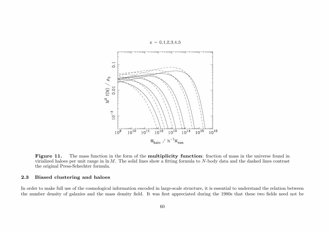
Figure 11. The mass function in the form of the multiplicity function: fraction of mass in the universe found invirialized haloes per unit range in lnM . The solid lines show a fitting formula to N -body data and the dashed lines contrastthe original Press-Schechter formula.

2.3 Biased clustering and haloes

In order to make full use of the cosmological information encoded in large-scale structure, it is essential to understand the relation betweenthe number density of galaxies and the mass density field. It was first appreciated during the 1980s that these two fields need not be

60

strictly proportional, starting with attempts to reconcile the Ωm = 1 Einstein–de Sitter model with observations. Although M/L ratios inrich clusters argued for dark matter, as first shown by Zwicky (1933), typical blue values of M/L � 300h implied only Ωm � 0.2 if theywere taken to be universal. Those who argued that the value Ωm = 1 was more natural (a greatly increased camp after the advent ofinflation) were therefore forced to postulate that the efficiency of galaxy formation was enhanced in dense environments: biased galaxyformation.

An argument for bias at the opposite extreme of density arose through the discovery of large voids in the galaxy distribution(Kirshner et al. 1981). There was a reluctance to believe that such vast regions could be truly devoid of matter – although this was at atime before the discovery of large-scale velocity fields.

What seemed to be required was a galaxy correlation function that was an amplified version of that for mass. This was exactly thephenomenon analysed for Abell clusters by Kaiser (1984), and thus was born the idea of high-peak bias: bright galaxies form only at thesites of high peaks in the initial density field. This was developed in some analytical detail by Bardeen et al. (1986), and was implementedin the simulations of Davis et al. (1985).

As shown below, the high-peak model produces a linear amplification of large-wavelength modes. This is likely to be a generalfeature of other models for bias, so it is useful to introduce the linear bias parameter:(

δρ

ρ

)galaxies

= b

(δρ

ρ

)mass

. (154)

This seems a reasonable assumption when δρ/ρ� 1, although it leaves open the question of how the effective value of b would be expectedto change on nonlinear scales. Galaxy clustering on large scales therefore allows us to determine mass fluctuations only if we know thevalue of b. When we observe large-scale galaxy clustering, we are only measuring b2ξmass(r) or b

2Δ2mass(k).

the peak-background split We now consider the central mechanism of biased clustering, in which a rare high density fluctuation,corresponding to a massive object, collapses sooner if it lies in a region of large-scale overdensity. This ‘helping hand’ from the long-wavelength modes means that overdense regions contain an enhanced abundance of massive objects with respect to the mean, so that thesesystems display enhanced clustering. The basic mechanism can be immediately understood via the diagram in figure 12; it was first clearlyanalysed by Kaiser (1984) in the context of rich clusters of galaxies. What Kaiser did not do was consider the degree of bias that applies

61

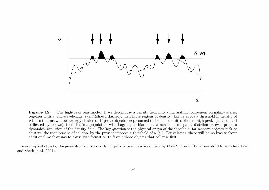
δ=νσ

δ

x

Figure 12. The high-peak bias model. If we decompose a density field into a fluctuating component on galaxy scales,together with a long-wavelength ‘swell’ (shown dashed), then those regions of density that lie above a threshold in density ofν times the rms will be strongly clustered. If proto-objects are presumed to form at the sites of these high peaks (shaded, andindicated by arrows), then this is a population with Lagrangian bias – i.e. a non-uniform spatial distribution even prior todynamical evolution of the density field. The key question is the physical origin of the threshold; for massive objects such asclusters, the requirement of collapse by the present imposes a threshold of ν >∼ 2. For galaxies, there will be no bias withoutadditional mechanisms to cause star formation to favour those objects that collapse first.

to more typical objects; the generalization to consider objects of any mass was made by Cole & Kaiser (1989; see also Mo & White 1996and Sheth et al. 2001).

62

The key ingredient of this analysis is the mass function of dark-matter haloes. The universe fragments into virialized systems suchthat f(M) dM is the number density of haloes in the mass range dM ; conservation of mass requires that

∫M f(M) dM = ρ0. A convenient

related dimensionless quantity is therefore the multiplicity function, M2f(M)/ρ0, which gives the fraction of the mass of the universecontained in haloes of a unit range in lnM . The simplest analyses of the mass function rest on the concept of a density threshold: collapseto a virialized object is deemed to have occurred where linear-theory δ averaged over a box containing mass M reaches some critical valueδc. Generally, we shall assume the value δc = 1.686 appropriate for spherical collapse in an Einstein–de Sitter universe. Now imagine thatthis situation is perturbed, by adding some constant shift ε to the density perturbations over some large region. The effect of this is toperturb the threshold: fluctuations now only need to reach δ = δc − ε in order to achieve collapse.

This change of threshold will increase the total collapse fraction on a given mass scale:

F → F − (dF/dδc) ε. (155)

Since ν = δc/σ(M), d/dδc = (1/σ)(d/dν) = (ν/δc)(d/dν), this is

F → F − (dF/d ln ν) ε/δc. (156)

To find the impact on the clustering of objects at a given mass scale, differentiate again with respect to ln ν and use the relation to themultiplicity function

M2f(M)/ρ0 = (d ln ν/d lnM) |dF/d ln ν|. (157)

So the mass function is proportional to the positive quantity G ≡ −dF/d ln ν, which is perturbed as follows:

G→ G− (dG/d ln ν) ε/δc. (158)

This gives a bias in the number density of haloes in Lagrangian space: δG/G = bLε, where the Lagrangian bias is

bL = −d lnGd ln ν

/δc. (159)

63

In addition to this modulation of the halo properties, the large-scale disturbance will move haloes closer together where ε is large,giving a density contrast of 1 + ε. If ε � 1, the overall fractional density contrast of haloes is therefore the sum of the dynamical andstatistical effects: δhalo = ε+ bLε. The overall bias in Eulerian space (b = δhalo/ε) is therefore

b = 1− d lnG

d ln ν/δc. (160)

Of course, the field ε can hardly be imposed by hand; instead, we make the peak-background split, in which δ is mentally decomposedinto a small-scale and a large-scale component – which we identify with ε. The scale above which the large-scale component is defined doesnot matter so long as it lies between the sizes of collapsed systems and the scales at which we wish to measure correlations.

From this point of view, it is clear that the mean bias should come out as unity when we average over all haloes: in this limit, werecover the full fluctuating mass density field. Thus we wish to find 〈b〉 = ∫

b(M)M f(M) dM/ρ0, weighting each halo by mass. From thedefinition of the mass function, this is

〈b〉 =∫b(M) dF = 1 +

∫(d lnG/d ln ν)Gd ln ν / δc. (161)

The latter integral is proportional to the difference in G between infinite mass and zero mass, which vanishes if the mass function vanishesin these limits.

To apply this apparatus, we need an explicit expression for the mass function. The simplest alternative is the original expression ofPress & Schechter (1974), which can be written in terms of the parameter ν = δc/σ(M):

G(ν) =

√2

πν exp

(−ν

2

2

). (162)

We now use d/dδc = σ(M)−1(d/dν) = (ν/δc)(d/dν), since M is not affected by the threshold change, which yields

b(ν) = 1 +ν2 − 1

δc. (163)

64

This says that M∗ haloes are unbiased, low-mass haloes are antibiased and high-mass haloes are positively biased, eventually reaching theb = ν/σ value expected for high peaks. The corresponding expression can readily be deduced for more accurate fitting formulae for themass function, such as that of Sheth & Tormen (1999):

G(ν) = 0.21617[1 + (√2/ν2)0.3] ν exp[−ν2/(2

√2)]. (164)

As stated earlier, an even better approximation is

F (> ν) = (1 + a νb)−1 exp(−c ν2), (165)

where (a, b, c) = (1.529, 0.704, 0.412)

We can now understand the observation that Abell clusters are much more strongly clustered than galaxies in general: regionsof large-scale overdensity contain systematically more high-mass haloes than expected if the haloes traced the mass. This phenomenonwas dubbed natural bias by White et al. (1987). However, applying the idea to galaxies is not straightforward: we have shown thatenhanced clustering is only expected for massive fluctuations with σ <

∼ 1, but galaxies at z = 0 fail this criterion. The high-peak ideaapplies will at high redshift, where massive galaxies are still assembling, but today there has been time for galaxy-scale haloes to collapsein all environments. The large bias that should exist at high redshifts is erased as the mass fluctuations grow: if the Lagrangian componentto the biased density field is kept unaltered, then the present-day bias will tend to unity as

b(ν) = 1 +ν2 − 1

(1 + zf )δc. (166)

(Fry 1986; Tegmark & Peebles 1998). Strong galaxy bias at z = 0 therefore requires some form of selection that locates present-day galaxiespreferentially in the rarer haloes with M > M∗ (Kauffmann, Nusser & Steinmetz 1997).

This dilemma forced the introduction of the idea of high-peak bias: bright galaxies form only at the sites of high peaks in theinitial density field (Bardeen et al. 1986; Davis et al. 1985). This idea is commonly, but incorrectly, attributed to Kaiser (1984), but itneeds an extra ingredient, namely a non-gravitational threshold. Attempts were therefore made to argue that the first generation of objectscould propagate disruptive signals, causing neighbours in low-density regions to be ‘still-born’. It is then possible to construct models (e.g.Bower et al. 1993) in which the large-scale modulation of the galaxy density is entirely non-gravitational in nature. However, it turned out

65

to be hard to make such mechanisms operate: the energetics and required scale of the phenomenon are very large (Rees 1985; Dekel & Rees1987). These difficulties were only removed when the standard model became a low-density universe, in which the dynamical argument forhigh galaxy bias no longer applied.

66

3 The hot big bang

3.1 Thermal history

Although the timescale for expansion of the early universe is very short, the density is also very high, so it is normally sensible to assumethat conditions are close to thermal equilibrium. Also the fluids of interest are simple enough that we can treat them as perfect gases. Thethermodynamics of such a gas is derived staring with a box of volume V = L3, and expanding the fields inside into periodic waves withharmonic boundary conditions. The density of states in k space is

dN = gV

(2π)3d3k (167)

(where g is a degeneracy factor for spin etc.). The equilibrium occupation number for a quantum state of energy ε is given generallyby

〈f〉 =[e(ε−μ)/kT ± 1

]−1

(168)

(+ for fermions, − for bosons). Now, for a thermal radiation background, the chemical potential, μ is always zero. The reason forthis is quite simple: μ appears in the first law of thermodynamics as the change in energy associated with a change in particle number,dE = TdS − PdV + μdN . So, as N adjusts to its equilibrium value, we expect that the system will be stationary with respect to smallchanges in N . The thermal equilibrium background number density of particles is

n =1

V

∫f dN = g

1

(2πh)3

∫ ∞

0

4π p2dp

eε(p)/kT ± 1, (169)

where we have changed to momentum space; ε =√m2c4 + p2c2 and g is the degeneracy factor. There are two interesting limits of this

expression.

67

(1) Ultrarelativistic limit. For kT � mc2 the particles behave as if they were massless, and we get

n =

(kT

c

)34πg

(2πh)3

∫ ∞

0

y2dy

ey ± 1. (170)

(2) Non-relativistic limit. Here we can neglect the ±1 in the occupation number, in which case the number is suppressed by a dominantexp(−mc2/kT ) factor:

n

nultrarel= (mc2/kT )3/2 exp(−mc2/kT )× [0.695 (F) 0.521 (B)]. (171)

This shows us that the background ‘switches on’ at about kT ∼ mc2; at this energy, known as a threshold, photons and otherspecies in equilibrium will have sufficient energy to create particle-antiparticle pairs.

The above thermodynamics also gives the energy density of the background, since it is only necessary to multiply the integrand bya factor ε(p) for the energy in each mode:

u = ρ c2 = g1

(2πh)3

∫ ∞

0

4π p2 dp

eε(p)/kT ± 1ε(p). (172)

In the ultrarelativistic limit, ε(p) = pc, this becomes

u =π2

30(hc)3g (kT )4 (bosons), (173)

and 7/8 of this for fermions.

68

If we are studying an adiabatic expansion, it will also be useful to know the entropy of the background. This is not too hardto work out, because energy and entropy are extensive quantities for a thermal background. Thus, writing the first law for μ = 0 and using∂S/∂V = S/V etc. for extensive quantities,

dE = TdS − PdV ⇒(E

VdV +

∂E

∂TdT

)=

(TS

VdV + T

∂S

∂TdT

)− PdV. (174)

Equating the dV and dT parts gives the familiar ∂E/∂T = T ∂S/∂T and

S =E + PV

T(175)

These results take an interesting and simple form in the ultrarelativistic limit. The energy density, u, obeys the usual black-bodyscaling u ∝ T 4. In the ultrarelativistic limit, we also know that the pressure is P = u/3, so that the entropy density is

s = (4/3)u/T =2π2k

45(hc)3g (kT )3 (bosons), (176)

and 7/8 of this for fermions. Now, we saw earlier that the number density of an ultrarelativistic background also scales as T 3 – thereforewe have the simple result that entropy just counts the number of particles. This justifies a common piece of terminology, in which the ratioof the number density of photons in the universe to the number density of baryons (protons plus neutrons) is called the entropy perbaryon. As we will see later, this ratio is about 109. The fact that this ratio is so large justifies the adiabatic assumption: pretty well allthe entropy is in the photons.

degrees of freedom Overall, the equilibrium relativistic density is

ρc2 =π2

30(hc)3geff (kT )

4; geff ≡∑

bosons

gi +7

8

∑fermions

gj , (177)

69

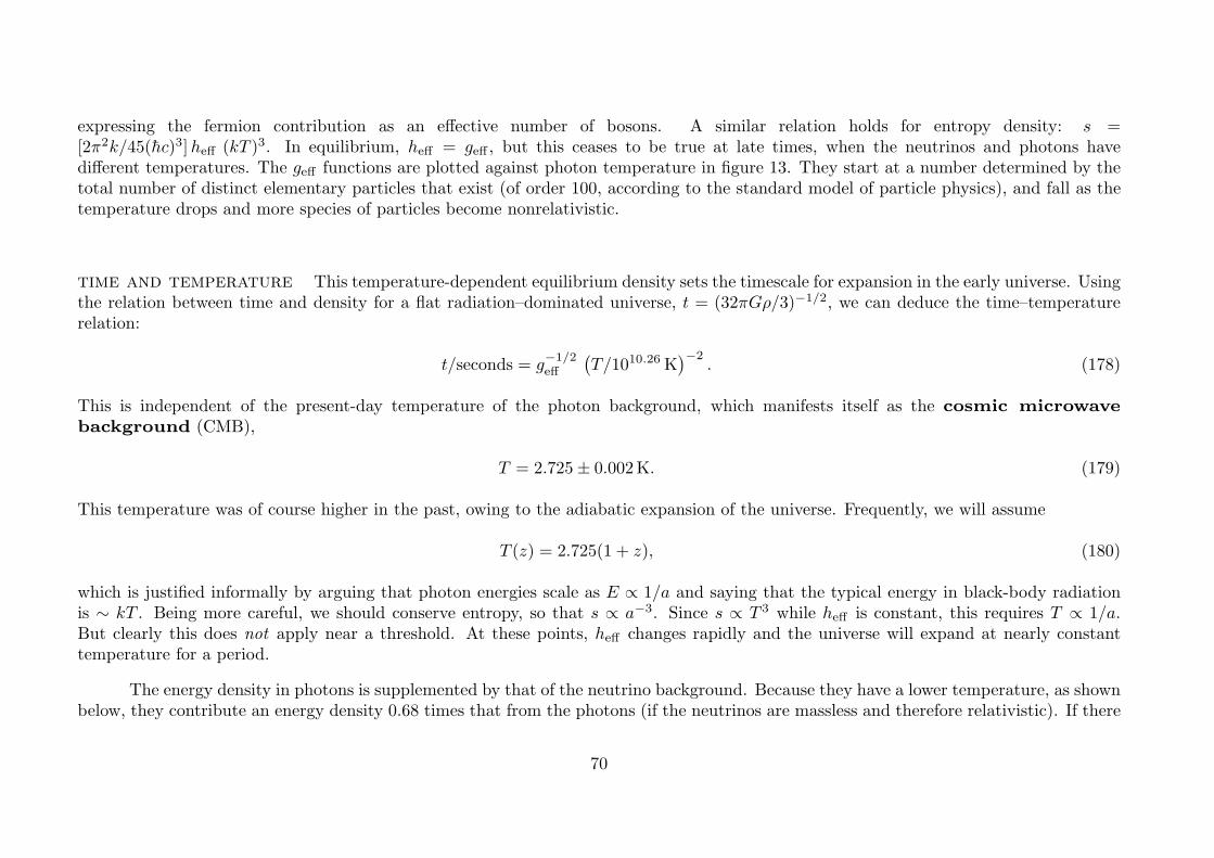
expressing the fermion contribution as an effective number of bosons. A similar relation holds for entropy density: s =[2π2k/45(hc)3]heff (kT )3. In equilibrium, heff = geff , but this ceases to be true at late times, when the neutrinos and photons havedifferent temperatures. The geff functions are plotted against photon temperature in figure 13. They start at a number determined by thetotal number of distinct elementary particles that exist (of order 100, according to the standard model of particle physics), and fall as thetemperature drops and more species of particles become nonrelativistic.

time and temperature This temperature-dependent equilibrium density sets the timescale for expansion in the early universe. Usingthe relation between time and density for a flat radiation–dominated universe, t = (32πGρ/3)−1/2, we can deduce the time–temperaturerelation:

t/seconds = g−1/2eff

(T/1010.26K

)−2. (178)

This is independent of the present-day temperature of the photon background, which manifests itself as the cosmic microwavebackground (CMB),

T = 2.725± 0.002K. (179)

This temperature was of course higher in the past, owing to the adiabatic expansion of the universe. Frequently, we will assume

T (z) = 2.725(1 + z), (180)

which is justified informally by arguing that photon energies scale as E ∝ 1/a and saying that the typical energy in black-body radiationis ∼ kT . Being more careful, we should conserve entropy, so that s ∝ a−3. Since s ∝ T 3 while heff is constant, this requires T ∝ 1/a.But clearly this does not apply near a threshold. At these points, heff changes rapidly and the universe will expand at nearly constanttemperature for a period.

The energy density in photons is supplemented by that of the neutrino background. Because they have a lower temperature, as shownbelow, they contribute an energy density 0.68 times that from the photons (if the neutrinos are massless and therefore relativistic). If there

70

Figure 13. The number of relativistic degrees of freedom as a function of photon temperature. geff measures the energydensity; heff the entropy (dashed line). The two depart significantly at low temperatures, when the neutrinos are coolerthan the photons. For a universe consisting only of photons, we would expect g = 2. The main features visible are (1) Theelectroweak phase transition at 100 Gev; (2) The QCD phase transition at 200 MeV; (3) the e± annihilation at 0.3 MeV.

are no other contributions to the energy density from relativistic particles, then the total effective radiation density is Ωrh2 � 4.2 × 10−5

and the redshift of matter–radiation equality is

1 + zeq = 24 074Ωh2 (T/2.725K)−4. (181)

71

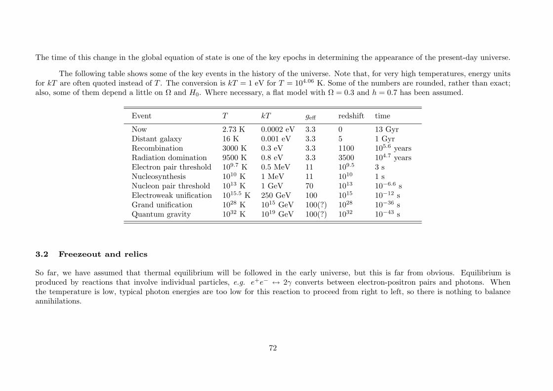
The time of this change in the global equation of state is one of the key epochs in determining the appearance of the present-day universe.

The following table shows some of the key events in the history of the universe. Note that, for very high temperatures, energy unitsfor kT are often quoted instead of T . The conversion is kT = 1 eV for T = 104.06 K. Some of the numbers are rounded, rather than exact;also, some of them depend a little on Ω and H0. Where necessary, a flat model with Ω = 0.3 and h = 0.7 has been assumed.

Event T kT geff redshift time

Now 2.73 K 0.0002 eV 3.3 0 13 GyrDistant galaxy 16 K 0.001 eV 3.3 5 1 GyrRecombination 3000 K 0.3 eV 3.3 1100 105.6 yearsRadiation domination 9500 K 0.8 eV 3.3 3500 104.7 yearsElectron pair threshold 109.7 K 0.5 MeV 11 109.5 3 sNucleosynthesis 1010 K 1 MeV 11 1010 1 sNucleon pair threshold 1013 K 1 GeV 70 1013 10−6.6 sElectroweak unification 1015.5 K 250 GeV 100 1015 10−12 sGrand unification 1028 K 1015 GeV 100(?) 1028 10−36 sQuantum gravity 1032 K 1019 GeV 100(?) 1032 10−43 s

3.2 Freezeout and relics

So far, we have assumed that thermal equilibrium will be followed in the early universe, but this is far from obvious. Equilibrium isproduced by reactions that involve individual particles, e.g. e+e− ↔ 2γ converts between electron-positron pairs and photons. Whenthe temperature is low, typical photon energies are too low for this reaction to proceed from right to left, so there is nothing to balanceannihilations.

72

Nevertheless, the annihilations only proceed at a finite rate: each member of the pair has to find a partner to interact with. We canexpress this by writing a simple differential equation for the electron density, called the Boltzmann equation:

n+ 3Hn = −〈σv〉n2 + S, (182)

where σ is the reaction cross-section, v is the particle velocity, and S is a source term that represents thermal particle production. The3Hn term just represents dilution by the expansion of the universe. Leaving aside the source term for the moment, we see that the changein n involves two timescales:

expansion timescale = H(z)−1

interaction timescale = (〈σv〉n)−1(183)

Both these times increase as the universe expands, but the interaction time usually changes fastest. Two-body reaction rates scaleproportional to density, times a cross-section that is often a declining function of energy, so that the interaction time changes at least asfast as R3. In contrast, the Hubble time changes no faster than R2 (in the radiation era), so that there is inevitably a crossover.

The situation therefore changes from one of thermal equilibrium at early times to a state of freezeout or decoupling at latetimes. Once the interaction timescale becomes much longer than the age of the universe, the particle has effectively ceased to interact. Itthus preserves a ‘snapshot’ of the properties of the universe at the time the particle was last in thermal equilibrium. This phenomenonof freezeout is essential to the understanding of the present-day nature of the universe. It allows for a whole set of relics to exist fromdifferent stages of the hot big bang. The photons of the microwave background are one such relic, generated at redshift z � 1100. A moreexotic example is the case of neutrinos.

To complete the Boltzmann equation, we need the source term S. This term can be fixed by a thermodynamic equilibrium argument:for a non-expanding universe, n will be constant at the equilibrium value for that temperature, nT , showing that

S = 〈σv〉n2T. (184)

73

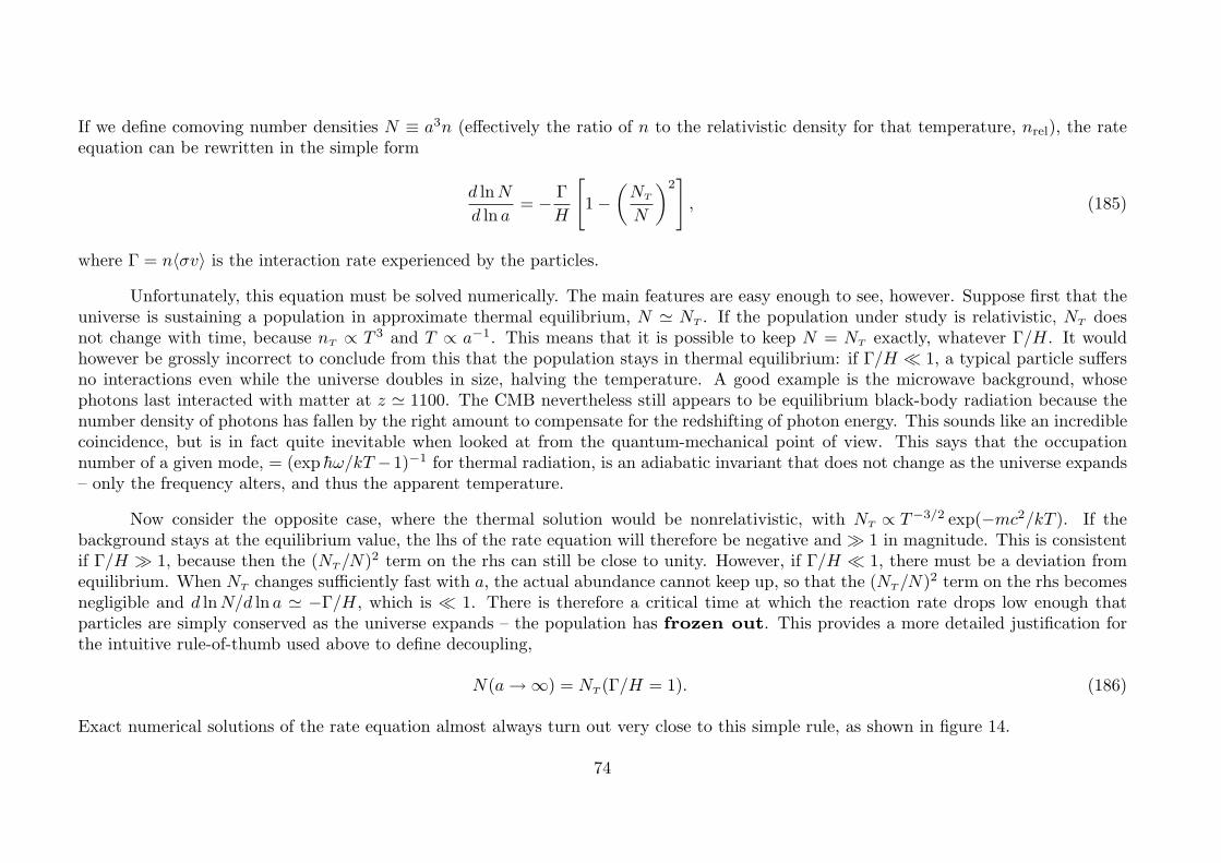
If we define comoving number densities N ≡ a3n (effectively the ratio of n to the relativistic density for that temperature, nrel), the rateequation can be rewritten in the simple form

d lnN

d ln a= − Γ

H

[1−

(NT

N

)2], (185)

where Γ = n〈σv〉 is the interaction rate experienced by the particles.Unfortunately, this equation must be solved numerically. The main features are easy enough to see, however. Suppose first that the

universe is sustaining a population in approximate thermal equilibrium, N � NT . If the population under study is relativistic, NT doesnot change with time, because nT ∝ T 3 and T ∝ a−1. This means that it is possible to keep N = NT exactly, whatever Γ/H. It wouldhowever be grossly incorrect to conclude from this that the population stays in thermal equilibrium: if Γ/H � 1, a typical particle suffersno interactions even while the universe doubles in size, halving the temperature. A good example is the microwave background, whosephotons last interacted with matter at z � 1100. The CMB nevertheless still appears to be equilibrium black-body radiation because thenumber density of photons has fallen by the right amount to compensate for the redshifting of photon energy. This sounds like an incrediblecoincidence, but is in fact quite inevitable when looked at from the quantum-mechanical point of view. This says that the occupationnumber of a given mode, = (exp hω/kT −1)−1 for thermal radiation, is an adiabatic invariant that does not change as the universe expands– only the frequency alters, and thus the apparent temperature.

Now consider the opposite case, where the thermal solution would be nonrelativistic, with NT ∝ T−3/2 exp(−mc2/kT ). If thebackground stays at the equilibrium value, the lhs of the rate equation will therefore be negative and � 1 in magnitude. This is consistentif Γ/H � 1, because then the (NT/N)

2 term on the rhs can still be close to unity. However, if Γ/H � 1, there must be a deviation fromequilibrium. When NT changes sufficiently fast with a, the actual abundance cannot keep up, so that the (NT/N)

2 term on the rhs becomesnegligible and d lnN/d ln a � −Γ/H, which is � 1. There is therefore a critical time at which the reaction rate drops low enough thatparticles are simply conserved as the universe expands – the population has frozen out. This provides a more detailed justification forthe intuitive rule-of-thumb used above to define decoupling,

N(a→∞) = NT (Γ/H = 1). (186)

Exact numerical solutions of the rate equation almost always turn out very close to this simple rule, as shown in figure 14.

74

Figure 14. Solution of the Boltzmann equation for freezeout of a single massive fermion. We set Γ/H = ε(kT/mc2)N/Nrel,as appropriate for a radiation-dominated universe in which 〈σv〉 is assumed to be independent of temperature. The solid linesshow the case ε = 1 and increasing by powers of 2. A high value of ε leads to freezeout at increasingly low abundances. Thedashed lines show the abundance predicted by the simple recipe of the thermal density for which Γ/H = 1.

the relic density The above freezeout criterion can be used to deduce a simple and very important expression for the present-daydensity of a non-relativistic relic:

Ωrelich2 � 10−41.5 (σ/m2)−1, (187)

75

so that only a small range of annihilation cross-sections will be of observational interest. The steps needed to get this formula are as follows.(1) From Γ/H = 1, the number density of relics at freezeout is nf = Hf/〈σv〉; (2) H = (8πGρ/3)1/2, where ρc2 = (π2/30h3c3)geff(kT )

4; (3)Ωrelic = 8πGmn0/3H

20 . The only missing ingredient here is how to relate the present number density n0 to the density nf at temperature

Tf . Since the relics are conserved, the number density must have fallen by the same factor as the entropy density:

nf/n0 = (hfeffT

3f )/(h

0effT

30 ). (188)

Today, h0eff = 43/11, and hf

eff = geff at high redshift. This allows us to deduce the relic density, given the mass, cross-section and temperatureof freezeout:

Ωrelich2 � 10−33.0 m2

〈σv〉(mc2

kTf

)g−1/2eff . (189)

We see from figure 14 that mc2/kTf ∼ 10 with only a logarithmic dependence on reaction rate, which roughly cancels the last factor onthe rhs. Finally, since particles are nearly relativistic at freezeout, we set 〈σv〉 = σc to get our final estimate of the typical cross-sectionfor an interesting relic abundance. The eventual conclusion makes sense: the higher the cross-section, the longer the particle can stay inequilibrium, and the more effective annihilations can be in suppressing the number density. Note that, in detail, we need to worry aboutwhether the particle is a Majorana particle (i.e. its own antiparticle) or a Dirac particle where particles and antiparticles aredistinct.

neutrino decoupling The best case for application of this freezeout apparatus is to relic neutrinos. At the later stages of the bigbang, energies are such that only light particles survive in equilibrium: photons (γ), neutrinos (ν) and e+e− pairs. As the temperature fallsbelow Te = 109.7 K), the pairs will annihilate. Electrons can interact via either the electromagnetic or the weak interaction, so in principlethe annihilations might yield pairs of photons or neutrinos. However, in practice the weak reactions freeze out earlier, at T � 1010 K.

The effect of the electron-positron annihilation is therefore to enhance the numbers of photons relative to neutrinos. Strictly, whatis conserved in this process is the entropy . The entropy of an e± + γ gas is easily found by remembering that it is proportional to thenumber density, and that all three particle species have g = 2 (polarization or spin). The total is then

s(γ + e+ + e−) =11

4s(γ). (190)

76

Equating this to photon entropy at a new temperature gives the factor by which the photon temperature is enhanced with respect tothat of the neutrinos. Equivalently, given the observed photon temperature today, we infer the existence of a neutrino background with atemperature

Tν =

(4

11

)1/3

Tγ = 1.945K, (191)

for Tγ = 2.725 K. Although it is hard to see how such low energy neutrinos could ever be detected directly, their gravitation is certainlynot negligible: they contribute an energy density that is a factor (7/8)× (4/11)4/3 times that of the photons. For three neutrino species,this enhances the energy density in relativistic particles by a factor 1.68 (there are three different kinds of neutrinos, just as there are threeleptons: the μ and τ particles are heavy analogues of the electron).

massive neutrinos Although for many years the conventional wisdom was that neutrinos were massless, this assumption began tobe increasingly challenged around the end of the 1970s. Theoretical progress in understanding the origin of masses in particle physicsmeant that it was no longer natural for the neutrino to be completely devoid of mass. Also, there is now some experimental evidence thatneutrinos have a small non-zero mass. The consequences of this for cosmology could be quite profound, as relic neutrinos are expected tobe very abundant. The above section showed that n(ν + ν) = (3/4)n(γ; T = 1.95K). That yields a total of 113 relic neutrinos in everycm3 for each species. The density contributed by these particles is easily worked out provided the mass is small enough. If this is thecase, then the neutrinos were ultrarelativistic at decoupling and their statistics were those of massless particles. As the universe expands tokT < mνc

2, the total number of neutrinos is preserved. We therefore obtain the present-day mass density in neutrinos just by multiplyingthe zero-mass number density by mν , and the consequence for the cosmological density in light neutrinos is easily worked out to be

Ωνh2 =

∑mi

94.1 eV. (192)

The more complicated case of neutrinos that decouple when they are already nonrelativistic is studied below.

77

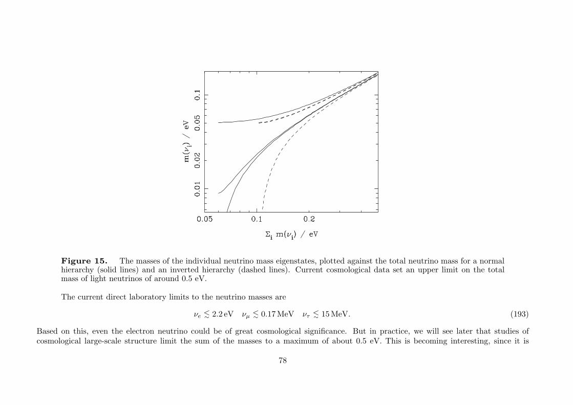
Figure 15. The masses of the individual neutrino mass eigenstates, plotted against the total neutrino mass for a normalhierarchy (solid lines) and an inverted hierarchy (dashed lines). Current cosmological data set an upper limit on the totalmass of light neutrinos of around 0.5 eV.

The current direct laboratory limits to the neutrino masses are

νe<∼ 2.2 eV νμ

<∼ 0.17MeV ντ

<∼ 15MeV. (193)

Based on this, even the electron neutrino could be of great cosmological significance. But in practice, we will see later that studies ofcosmological large-scale structure limit the sum of the masses to a maximum of about 0.5 eV. This is becoming interesting, since it is

78

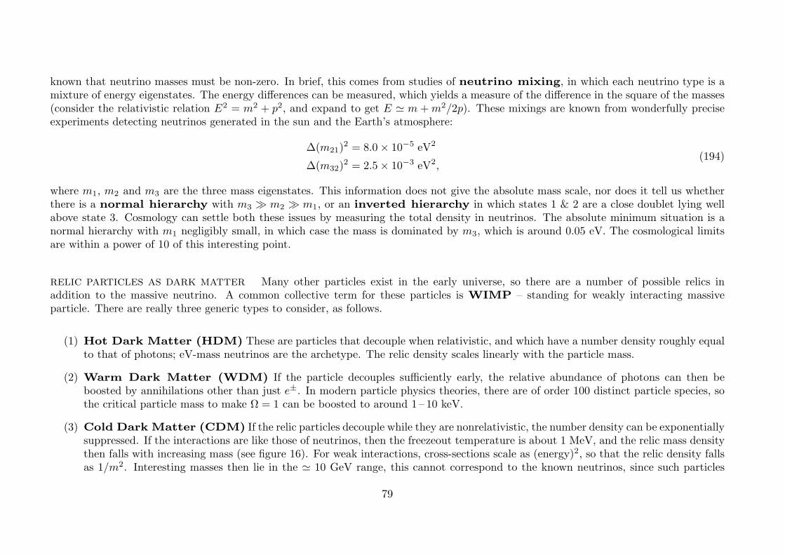
known that neutrino masses must be non-zero. In brief, this comes from studies of neutrino mixing, in which each neutrino type is amixture of energy eigenstates. The energy differences can be measured, which yields a measure of the difference in the square of the masses(consider the relativistic relation E2 = m2 + p2, and expand to get E � m +m2/2p). These mixings are known from wonderfully preciseexperiments detecting neutrinos generated in the sun and the Earth’s atmosphere:

Δ(m21)2 = 8.0× 10−5 eV2

Δ(m32)2 = 2.5× 10−3 eV2,

(194)

where m1, m2 and m3 are the three mass eigenstates. This information does not give the absolute mass scale, nor does it tell us whetherthere is a normal hierarchy with m3 � m2 � m1, or an inverted hierarchy in which states 1 & 2 are a close doublet lying wellabove state 3. Cosmology can settle both these issues by measuring the total density in neutrinos. The absolute minimum situation is anormal hierarchy with m1 negligibly small, in which case the mass is dominated by m3, which is around 0.05 eV. The cosmological limitsare within a power of 10 of this interesting point.

relic particles as dark matter Many other particles exist in the early universe, so there are a number of possible relics inaddition to the massive neutrino. A common collective term for these particles is WIMP – standing for weakly interacting massiveparticle. There are really three generic types to consider, as follows.

(1) Hot Dark Matter (HDM) These are particles that decouple when relativistic, and which have a number density roughly equalto that of photons; eV-mass neutrinos are the archetype. The relic density scales linearly with the particle mass.

(2) Warm Dark Matter (WDM) If the particle decouples sufficiently early, the relative abundance of photons can then beboosted by annihilations other than just e±. In modern particle physics theories, there are of order 100 distinct particle species, sothe critical particle mass to make Ω = 1 can be boosted to around 1 – 10 keV.

(3) Cold Dark Matter (CDM) If the relic particles decouple while they are nonrelativistic, the number density can be exponentiallysuppressed. If the interactions are like those of neutrinos, then the freezeout temperature is about 1 MeV, and the relic mass densitythen falls with increasing mass (see figure 16). For weak interactions, cross-sections scale as (energy)2, so that the relic density fallsas 1/m2. Interesting masses then lie in the � 10 GeV range, this cannot correspond to the known neutrinos, since such particles

79

Figure 16. The contribution to the density parameter produced by relic neutrinos (or neutrino-like particles) as afunction of their rest mass. The shaded band shows a factor of 2 either side of the observed CDM density. At low masses,the neutrinos are highly relativistic when they decouple: their abundance takes the zero-mass value, and the density is justproportional to the mass. Above about 1 MeV, the neutrinos are non-relativistic at decoupling, and their relic density isreduced by annihilation. Above the mass of the Z boson, the cross-section falls, so that annihilation is less effective and therelic density rises again.

would have been seen in accelerators. But beyond about 90 GeV (the mass of the Z boson), the strength of the weak interactionis reduced, with cross-section going as (energy)−2. The relic density now rises as m2, so that the observed dark matter density is

80

attained at m � 1 TeV. Plausible candidates of this sort are found among so-called supersymmetric theories, which predictmany new weakly-interacting particles. The favoured particle for a CDM relic is called the neutralino.

Since these particles exist to explain galaxy rotation curves, they must be passing through us right now. There is therefore a hugeeffort in the direct laboratory detection of dark matter, mainly via cryogenic detectors that look for the recoil of a single nucleon whenhit by a DM particle (in deep mines, to shield from cosmic rays). So far, there are no detections, but well-constructed experiments withlow backgrounds are starting to set interesting limits, as shown in figure 17. There is no unique target to aim for, since even the simplestexamples of supersymmetric models contain a variety of free parameters. These allow models that are optimistically close to current limits,but also some that will be hard to verify. The public-domain package DarkSUSY is available at www.physto.se/~edsjo/darksusy tomake these detailed abundance calculations.

What is particularly exciting is that the properties of these relic particles can also be observed via new examples manufactured inparticle accelerators. The most wonderful outcome would be for the same particle to be found in these two different ways. The chancesof success in this enterprise are hard to estimate, and some models exist in which detection would be impossible for many decades. Butit would be a tremendous scientific achievement if dark matter particles were to be detected in this way, and a good part of the plausibleparameter space will be covered over the next decade.

baryogenesis It should be emphasised that these freezeout calculations predict equal numbers of particles and antiparticles. Thismakes a critical contrast with the case of normal or baryonic material. The number density of baryons is low (roughly 10−9 that ofthe CMB photons), so one’s first thought might be that baryons are another frozen-out relic. But as far as is known, there is a negligiblecosmic density of antibaryons; even if antimatter existed, freezeout applied to protons-antiproton pairs predicts a density far below whatis observed. The inevitable conclusion is that the universe began with a very slight asymmetry between matter and antimatter: at hightemperatures there were 1 + O(10−9) protons for every antiproton. If baryon number is conserved, this imbalance cannot be altered onceit is set in the initial conditions; but what generates it? This is clearly one of the big challenges in cosmology, but our ideas are less wellformed here than in many other areas.

81

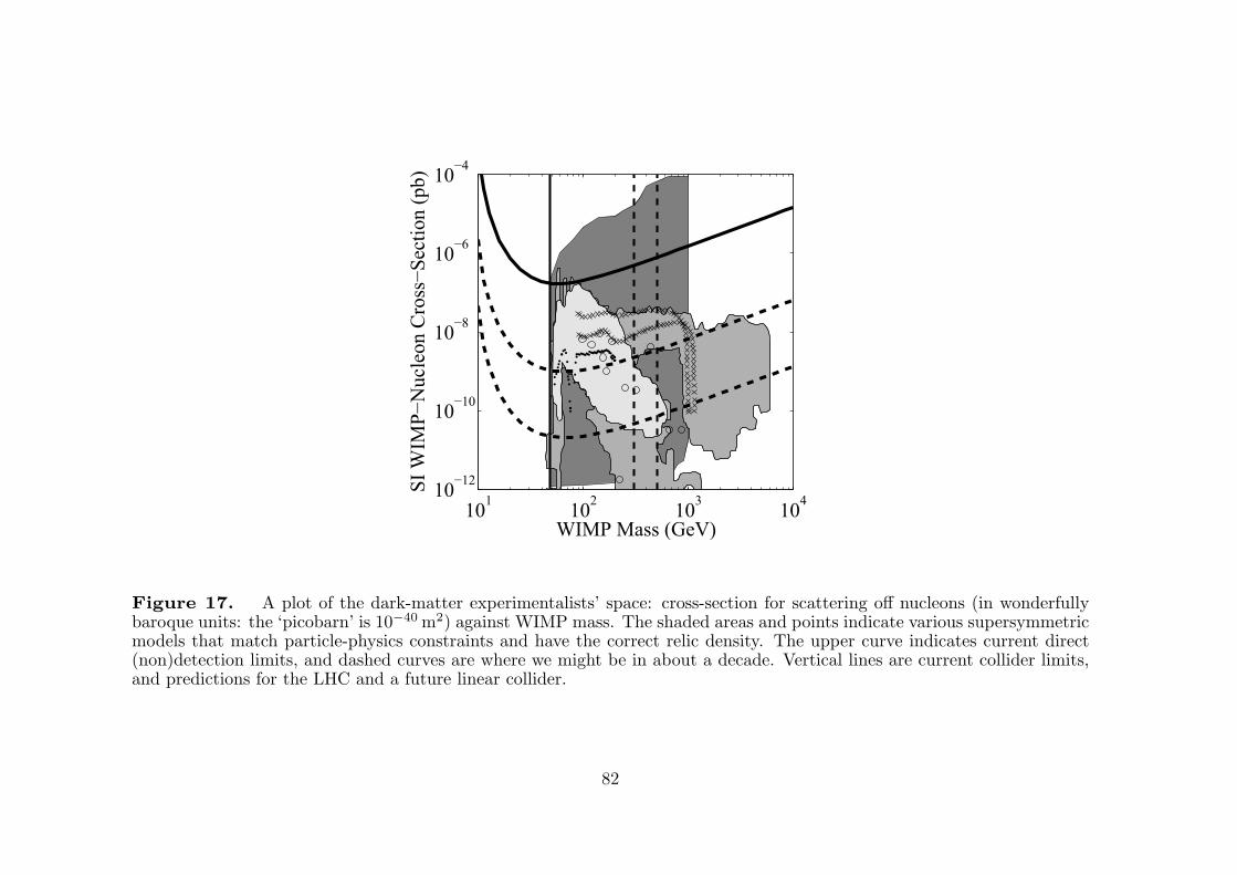
WIMP Mass (GeV)

SI W

IMP−

Nuc

leon

Cro

ss−S

ectio

n (p

b)

101 102 103 10410−12

10−10

10−8

10−6

10−4

Figure 17. A plot of the dark-matter experimentalists’ space: cross-section for scattering off nucleons (in wonderfullybaroque units: the ‘picobarn’ is 10−40m2) against WIMP mass. The shaded areas and points indicate various supersymmetricmodels that match particle-physics constraints and have the correct relic density. The upper curve indicates current direct(non)detection limits, and dashed curves are where we might be in about a decade. Vertical lines are current collider limits,and predictions for the LHC and a future linear collider.

82

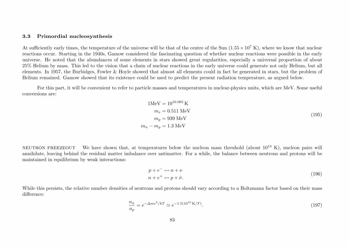
3.3 Primordial nucleosynthesis

At sufficiently early times, the temperature of the universe will be that of the centre of the Sun (1.55× 107 K), where we know that nuclearreactions occur. Starting in the 1940s, Gamow considered the fascinating question of whether nuclear reactions were possible in the earlyuniverse. He noted that the abundances of some elements in stars showed great regularities, especially a universal proportion of about25% Helium by mass. This led to the vision that a chain of nuclear reactions in the early universe could generate not only Helium, but allelements. In 1957, the Burbidges, Fowler & Hoyle showed that almost all elements could in fact be generated in stars, but the problem ofHelium remained. Gamow showed that its existence could be used to predict the present radiation temperature, as argued below.

For this part, it will be convenient to refer to particle masses and temperatures in nuclear-physics units, which are MeV. Some usefulconversions are:

1MeV = 1010.065K

me = 0.511 MeV

mp = 939 MeV

mn −mp = 1.3 MeV

(195)

neutron freezeout We have shown that, at temperatures below the nucleon mass threshold (about 1013 K), nucleon pairs willannihilate, leaving behind the residual matter imbalance over antimatter. For a while, the balance between neutrons and protons will bemaintained in equilibrium by weak interactions:

p+ e− ↔ n+ ν

n+ e+ ↔ p+ ν.(196)

While this persists, the relative number densities of neutrons and protons should vary according to a Boltzmann factor based on their massdifference:

nn

np= e−Δmc2/kT � e−1.5(1010 K/T ). (197)

83

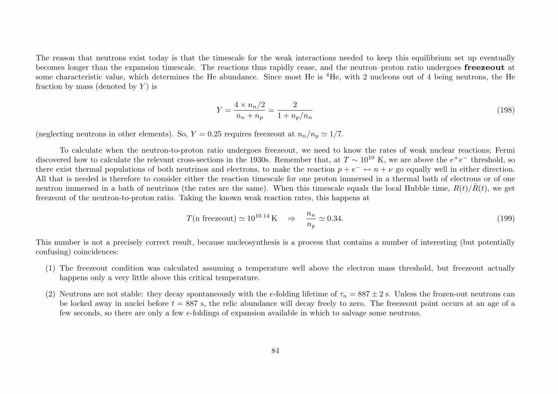
The reason that neutrons exist today is that the timescale for the weak interactions needed to keep this equilibrium set up eventuallybecomes longer than the expansion timescale. The reactions thus rapidly cease, and the neutron–proton ratio undergoes freezeout atsome characteristic value, which determines the He abundance. Since most He is 4He, with 2 nucleons out of 4 being neutrons, the Hefraction by mass (denoted by Y ) is

Y =4× nn/2

nn + np=

2

1 + np/nn(198)

(neglecting neutrons in other elements). So, Y = 0.25 requires freezeout at nn/np � 1/7.

To calculate when the neutron-to-proton ratio undergoes freezeout, we need to know the rates of weak nuclear reactions; Fermidiscovered how to calculate the relevant cross-sections in the 1930s. Remember that, at T ∼ 1010 K, we are above the e+e− threshold, sothere exist thermal populations of both neutrinos and electrons, to make the reaction p + e− ↔ n + ν go equally well in either direction.All that is needed is therefore to consider either the reaction timescale for one proton immersed in a thermal bath of electrons or of oneneutron immersed in a bath of neutrinos (the rates are the same). When this timescale equals the local Hubble time, R(t)/R(t), we getfreezeout of the neutron-to-proton ratio. Taking the known weak reaction rates, this happens at

T (n freezeout) � 1010.14K ⇒ nn

np� 0.34. (199)

This number is not a precisely correct result, because nucleosynthesis is a process that contains a number of interesting (but potentiallyconfusing) coincidences:

(1) The freezeout condition was calculated assuming a temperature well above the electron mass threshold, but freezeout actuallyhappens only a very little above this critical temperature.

(2) Neutrons are not stable: they decay spontaneously with the e-folding lifetime of τn = 887± 2 s. Unless the frozen-out neutrons canbe locked away in nuclei before t = 887 s, the relic abundance will decay freely to zero. The freezeout point occurs at an age of afew seconds, so there are only a few e-foldings of expansion available in which to salvage some neutrons.

84

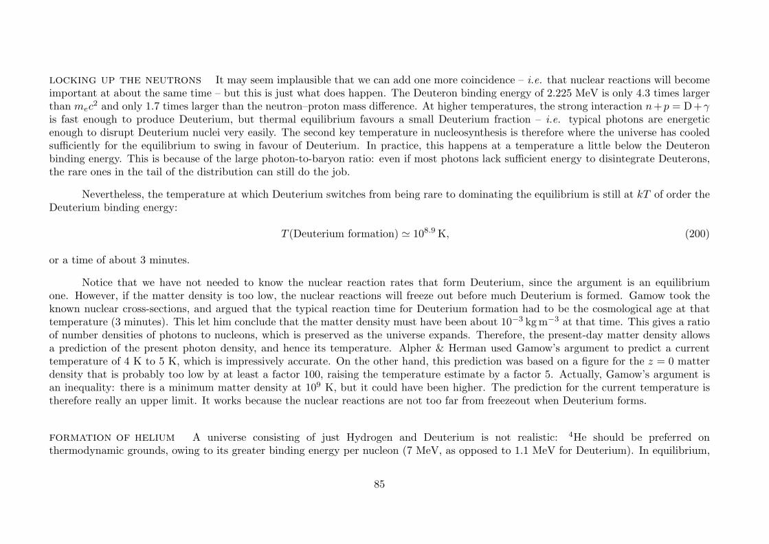
locking up the neutrons It may seem implausible that we can add one more coincidence – i.e. that nuclear reactions will becomeimportant at about the same time – but this is just what does happen. The Deuteron binding energy of 2.225 MeV is only 4.3 times largerthan mec

2 and only 1.7 times larger than the neutron–proton mass difference. At higher temperatures, the strong interaction n+p = D+γis fast enough to produce Deuterium, but thermal equilibrium favours a small Deuterium fraction – i.e. typical photons are energeticenough to disrupt Deuterium nuclei very easily. The second key temperature in nucleosynthesis is therefore where the universe has cooledsufficiently for the equilibrium to swing in favour of Deuterium. In practice, this happens at a temperature a little below the Deuteronbinding energy. This is because of the large photon-to-baryon ratio: even if most photons lack sufficient energy to disintegrate Deuterons,the rare ones in the tail of the distribution can still do the job.

Nevertheless, the temperature at which Deuterium switches from being rare to dominating the equilibrium is still at kT of order theDeuterium binding energy:

T (Deuterium formation) � 108.9K, (200)

or a time of about 3 minutes.

Notice that we have not needed to know the nuclear reaction rates that form Deuterium, since the argument is an equilibriumone. However, if the matter density is too low, the nuclear reactions will freeze out before much Deuterium is formed. Gamow took theknown nuclear cross-sections, and argued that the typical reaction time for Deuterium formation had to be the cosmological age at thattemperature (3 minutes). This let him conclude that the matter density must have been about 10−3 kgm−3 at that time. This gives a ratioof number densities of photons to nucleons, which is preserved as the universe expands. Therefore, the present-day matter density allowsa prediction of the present photon density, and hence its temperature. Alpher & Herman used Gamow’s argument to predict a currenttemperature of 4 K to 5 K, which is impressively accurate. On the other hand, this prediction was based on a figure for the z = 0 matterdensity that is probably too low by at least a factor 100, raising the temperature estimate by a factor 5. Actually, Gamow’s argument isan inequality: there is a minimum matter density at 109 K, but it could have been higher. The prediction for the current temperature istherefore really an upper limit. It works because the nuclear reactions are not too far from freezeout when Deuterium forms.

formation of helium A universe consisting of just Hydrogen and Deuterium is not realistic: 4He should be preferred onthermodynamic grounds, owing to its greater binding energy per nucleon (7 MeV, as opposed to 1.1 MeV for Deuterium). In equilibrium,

85

the abundance of 4He relative to protons should reach unity at an energy of about 0.3 MeV, at which point the relative abundance ofDeuterium should be only ∼ 10−12.

Since the simplest way to synthesize Helium is by fusing Deuterium, the production of Helium must in practice await the synthesisof significant quantities of Deuterium. Nevertheless, the Deuterium will be rapidly converted to Helium once significant nucleosynthesisbegins. This argument is what allows us to expect that the Helium abundance can be calculated from the final n/p ratio. The processstarts by fusing Deuterium to make either Tritium and 3He, following which there are four main ways of reaching 4He (leaving aside rarerreactions involving residual free neutrons):

D + D = 3He + n

D+D = T+ p

D+D = 4He

T + p = 4He

D + 3He = 4He + p

T+D = 4He + n.

(201)

A universe that stayed in nuclear equilibrium as it cooled would eventually consist entirely of Iron, since this has the highest bindingenergy per nucleon. However, by the time Helium synthesis is accomplished, the density and temperature are too low for significant synthesisof heavier nuclei to proceed. Apart from Helium, the main nuclear residue of the big bang is therefore those Deuterium nuclei that escapebeing mopped up into Helium, plus a trace of 3He. The other intermediate product, Tritium, is not so strongly bound and thus leaves nosignificant relic. There also exist extremely small fractions of other elements: 7Li (∼ 10−9 by mass) and 7Be (∼ 10−11).

In summary, nucleosynthesis starts at about 1010 K, when the universe was about 1 s old, and effectively ends when it has cooledby a factor of 10, and is about 100 times older.

86

the number of particle generations An accurate fit for the final neutron-to-proton ratio is

nn

np� 0.163 (ΩBh

2)0.04 (Nν/3)0.2. (202)

The signs of the dependences on the baryon density and on the number of neutrino species are easily understood. A high baryon densityincreases the temperature at which nuclei form and gives a higher neutron abundance because fewer of them have decayed. This is a weakeffect, because the neutron fraction is largely set by weak-interaction freeze-out, which is independent of the baryon density. The effect ofextra neutrino species is to boost the total relativistic density. This increase the overall rate of expansion, so that weak-interaction freezeouthappens earlier and thus at higher T , again raising the neutron abundance.

It is therefore clear that strong limits can be set on the number of unobserved neutrino species, and thus on the number of possibleadditional families in particle physics. For many years, these nucleosynthesis limits were stronger than those that existed from particlephysics experiments. This changed in 1990, with a critical series of experiments carried out in the LEP (large electron-positron) colliderat CERN, which was the first experiment to produce Z0 particles in large numbers. The Z0 can decay to pairs of neutrinos so long as theirrest mass sums to less than 91.2 GeV; more species increase the decay rate, and decrease the Z0 lifetime. Since 1990, these argumentshave required N to be very close to 3; it is a matter of detailed argument over the Helium data as to whether N = 4 was ruled out fromcosmology prior to this.

weighing the baryons Unlike Helium, the relic abundances of the other light elements are rather sensitive to density. We haveseen that Helium formation occurs at very nearly a fixed temperature, depending only weakly on density or neutrino species. The residualDeuterium will therefore freeze out at about this temperature, leaving a number density fixed at whatever sets the reaction rate low enoughto survive for a Hubble time. Since this density is a fixed quantity, the proportion of the baryonic density that survives as Deuterium (or3He) should thus decline roughly as 1/(density).

This provides a relatively sensitive means of weighing the baryonic content of the universe. A key event in the development ofcosmology was thus the determination of the D/H ratio in the interstellar medium, carried out in the early 1970s. This gave D/H � 2×10−5,providing the first evidence for a low baryonic density, as follows. Figure 18 shows how the abundances of light elements vary with the

87

cosmological density, according to detailed calculations. The baryonic density in these calculations is traditionally quoted in the field asthe reciprocal of the entropy per baryon:

η ≡ (np + nn)/nγ = 2.74× 10−8(T/2.73K)−3ΩBh2. (203)

Figure 18 shows that this Deuterium abundance favours a low density:

ΩBh2 � 0.02± 0.002. (204)

(although lower values are favoured if a higher weight is given to the Helium abundance). Baryons therefore cannot close the universe. IfΩ = 1, the dark matter must be non-baryonic.

3.4 Recombination

Moving closer to the present, and passing through matter-radiation equality at z ∼ 104, the next critical epoch in the evolution of theuniverse is reached when the temperature drops to the point (T ∼ 1000 K) where it is thermodynamically favourable for the ionized plasmato form neutral atoms. This process is known as recombination: a complete misnomer, as the plasma has always been completelyionized up to this time.

the rate equation A natural first thought is that the ionization of the plasma may be treated by a thermal-equilibrium approach,using the Saha equation, which applies in stellar atmospheres. In fact, such an approach is almost always invalid. This is not becauseelectromagnetic interactions are too slow to maintain equilibrium: rather, they are too fast. Consider a single recombination; if this were tooccur directly to the ground state, a photon with hω > χ would be produced. Such photons are almost immediately destroyed by ionizinganother neutral atom. Similarly, reaching the ground state requires the production of photons at least as energetic as the 2P → 1S spacing(Lyman α, with λ = 1216A), and these also are re-absorbed very efficiently. This is a common phenomenon in astrophysics: the Lyman αphotons undergo resonant scattering and are very hard to get rid of (unlike a finite HII region, where the Lyα photons can escape).

88

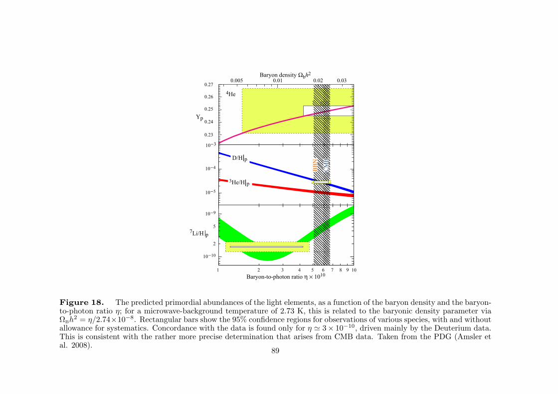
3He/H p

4He

2 3 4 5 6 7 8 9 101

0.01 0.02 0.030.005

CM

B

BB

N

Baryon-to-photon ratio η × 1010

Baryon density Ωbh2

D___H

0.24

0.23

0.25

0.26

0.27

10−4

10−3

10−5

10−9

10−10

2

57Li/H p

Yp

D/H p

Figure 18. The predicted primordial abundances of the light elements, as a function of the baryon density and the baryon-to-photon ratio η; for a microwave-background temperature of 2.73 K, this is related to the baryonic density parameter viaΩBh

2 = η/2.74×10−8. Rectangular bars show the 95% confidence regions for observations of various species, with and withoutallowance for systematics. Concordance with the data is found only for η � 3× 10−10, driven mainly by the Deuterium data.This is consistent with the rather more precise determination that arises from CMB data. Taken from the PDG (Amsler etal. 2008).

89

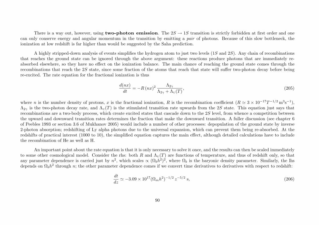
There is a way out, however, using two-photon emission. The 2S → 1S transition is strictly forbidden at first order and onecan only conserve energy and angular momentum in the transition by emitting a pair of photons. Because of this slow bottleneck, theionization at low redshift is far higher than would be suggested by the Saha prediction.

A highly stripped-down analysis of events simplifies the hydrogen atom to just two levels (1S and 2S). Any chain of recombinationsthat reaches the ground state can be ignored through the above argument: these reactions produce photons that are immediately re-absorbed elsewhere, so they have no effect on the ionization balance. The main chance of reaching the ground state comes through therecombinations that reach the 2S state, since some fraction of the atoms that reach that state will suffer two-photon decay before beingre-excited. The rate equation for the fractional ionization is thus

d(nx)

dt= −R (nx)2 Λ2γ

Λ2γ + ΛU(T ), (205)

where n is the number density of protons, x is the fractional ionization, R is the recombination coefficient (R � 3 × 10−17T−1/2m3s−1),Λ2γ is the two-photon decay rate, and ΛU(T ) is the stimulated transition rate upwards from the 2S state. This equation just says thatrecombinations are a two-body process, which create excited states that cascade down to the 2S level, from whence a competition betweenthe upward and downward transition rates determines the fraction that make the downward transition. A fuller discussion (see chapter 6of Peebles 1993 or section 3.6 of Mukhanov 2005) would include a number of other processes: depopulation of the ground state by inverse2-photon absorption; redshifting of Ly alpha photons due to the universal expansion, which can prevent them being re-absorbed. At theredshifts of practical interest (1000 to 10), the simplified equation captures the main effect, although detailed calculations have to includethe recombination of He as well as H.

An important point about the rate equation is that it is only necessary to solve it once, and the results can then be scaled immediatelyto some other cosmological model. Consider the rhs: both R and ΛU(T ) are functions of temperature, and thus of redshift only, so thatany parameter dependence is carried just by n2, which scales ∝ (Ωbh

2)2, where Ωb is the baryonic density parameter. Similarly, the lhsdepends on Ωbh

2 through n; the other parameter dependence comes if we convert time derivatives to derivatives with respect to redshift:

dt

dz� −3.09× 1017(Ωmh

2)−1/2 z−5/2 s, (206)

90

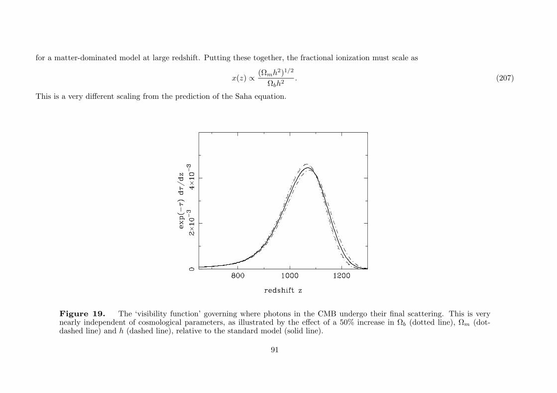
for a matter-dominated model at large redshift. Putting these together, the fractional ionization must scale as

x(z) ∝ (Ωmh2)1/2

Ωbh2. (207)

This is a very different scaling from the prediction of the Saha equation.

Figure 19. The ‘visibility function’ governing where photons in the CMB undergo their final scattering. This is verynearly independent of cosmological parameters, as illustrated by the effect of a 50% increase in Ωb (dotted line), Ωm (dot-dashed line) and h (dashed line), relative to the standard model (solid line).

91

last scattering Recombination is important observationally because it marks the first time that photons can travel freely. Whenthe ionization is high, Thomson scattering causes them to proceed in a random walk, so the early universe is opaque. The interesting thingfrom our point of view is to work out the maximum redshift from which we can receive a photon without it suffering scattering. To do this,we work out the optical depth to Thomson scattering,

τ =

∫nexσTd�proper; d�proper = R(z) dr = R0 dr/(1 + z). (208)

For a fully ionized plasma with 25% He by mass, the electron number density is

ne(z) = 9.83Ωbh2 (1 + z)3 m−3. (209)

Also, d�proper = c dt, which brings in a factor of (Ωmh2)−1/2. These two density terms automatically cancel the principal dependence of

x(z), so we predict that the optical depth should be very largely a function of redshift only. For standard parameters, a good approximationaround τ = 1 is

τ(z) �(1 + z

1080

)13

(210)

(cf. Jones & Wyse 1985).

This approximation is not perfect, however, and very accurate work needs detailed numerical solution of the evolution equations,including the omitted processes. See Seager, Sasselov & Scott (2000; ApJS, 128, 407). Because τ changes rapidly with redshift, thevisibility function for the redshift at which photons were last scattered, e−τdτ/dz, is sharply peaked, and is well fitted by a Gaussianof mean redshift 1070 and standard deviation in redshift 80. As illustrated in figure 19, these properties are in practice insensitive tothe cosmological parameters. Thus, when we look at the sky, we can expect to see in all directions photons that originate from a last-scattering surface at z � 1100. It is worth noting that this redshift is very much lower than we would expect just from setting

k × 2.725 K× (1 + z) = χ, (211)

which gives z � 104.8. The difference is partly because the ionization falls slower than Saha, but also because even a tiny ionization easilycauses scattering. The fact that the properties of the last-scattering surface are almost independent of all the unknowns in cosmology isimmensely satisfying, and gives us at least one relatively solid piece of ground to act as a base in exploring the trackless swamp of cosmology.

92

4 Frontiers

In the remaining time, we survey some of the big questions raised by the standard model of cosmology, in the hope that subsequent lecturerswill be able to answer them satisfactorily.

4.1 Initial condition problems

The expanding universe of the big-bang model is surprising in many ways: (1) What caused the expansion? (2) Why is the expansion soclose to flat – i.e. Ω ∼ 1 today? (3) Why is the universe close to isotropic (the same in all directions)? (4) Why does it contain structure?Some of these problems may seem larger than others, but when examined in detail all point to something missing in our description ofthe early stages of cosmological history. It is normally assumed that the solution to this will be some piece of additional physics that isimportant at high energies. Before discussing possibilities, there are a few important general ideas that will be needed.

quantum gravity limit In principle, T → ∞ as R → 0, but there comes a point at which this extrapolation of classical physicsbreaks down. This is where the thermal energy of typical particles is such that their de Broglie wavelength is smaller than their Schwarzschildradius: quantum black holes clearly cause difficulties with the usual concept of background spacetime. Equating 2πh/(mc) to 2Gm/c2

yields a characteristic mass for quantum gravity known as the Planck mass. This mass, and the corresponding length h/(mPc) and time�P/c form the system of Planck units:

mP ≡√hc

G� 1019GeV

�P ≡√hG

c3� 10−35m

tP ≡√hG

c5� 10−43s.

(212)

93

The Planck time therefore sets the origin of time for the classical phase of the big bang. It is incorrect to extend the classical solution toR = 0 and conclude that the universe began in a singularity of infinite density. A common question about the big bang is ‘what happenedat t < 0?’, but in fact it is not even possible to get to zero time without adding new physical laws.

natural units To simplify the appearance of equations, it is common practice in high-energy physics to adopt natural units, wherewe take

k = h = c = μ0 = ε0 = 1. (213)

This convention makes the meaning of equations clearer by reducing the algebraic clutter, and is also useful in the construction of intuitivearguments for the order of magnitude of quantities of interest. In the professional world of cosmology, natural units are frequently adoptedwithout comment, so this is something to watch out for. Hereafter, natural units will frequently be adopted, although it will occasionallybe convenient to re-insert explicit powers of h etc.

The adoption of natural units corresponds to fixing the units of charge, mass, length and time relative to each other. This leavesone free unit, usually taken to be energy. Natural units are thus one step short of the Planck system, in which G = 1 also, so that all unitsare fixed and all physical quantities are dimensionless. In natural units, the following dimensional equalities hold:

[E] = [T ] = [m]

[L] = [m]−1(214)

Hence, the dimensions of energy density are

[u] = [m]4, (215)

with units often quoted in GeV4. It is however often of interest to express things in Planck units: energy as a multiple of mP, energydensity as a multiple of m4

Petc. The gravitational constant itself is then

G = m−2P. (216)

94

flatness problem Now to quantify the first of the many puzzles concerning initial conditions. From the Friedmann equation, we canwrite the density parameter as a function of era:

Ω(a) =8πGρ(a)

H2(a)=

Ωv +Ωma−3 +Ωra

−4

Ωv +Ωma−3 +Ωra−4 − (Ω− 1)a−2(217)

(and corresponding expressions for the Ω(a) corresponding to any one component just by picking the appropriate term on the top line).This tells us that, if the total Ω is unity today, it was always unity (a geometrical statement: if k = 0, it can’t make a continuous transitionto k = ±1). But if Ω = 1, how does Ω(a) evolve? It should be clear that Ω(a)→ 1 at very large and very small a, provided Ωv is nonzero inthe former case, and provided Ωm or Ωr is nonzero in the latter case (without vacuum energy, Ω = 1 is unstable). In short, the Ω = 1 stateis an attractor, looking in either direction in time. It has long been clear that this presents a puzzle with regard to the initial conditions.These will be radiation dominated, so we have

Ω(ainit) � 1 +(Ω− 1)

Ωra2init. (218)

If we are willing to consider a Planck-scale origin with ainit ∼ 10−32, then clearly conditions at that time must be flat to perhaps 60 powersof 10. A more democratic initial condition might be thought to have Ω − 1 of order unity, so some mechanism to make it very small (orzero) is clearly required. This ‘how could the universe have known?’ argument is a general basis for a prejudice that Ω = 1 holds exactlytoday: it would seem contrived for the expansion to have proceeded for so many powers of 10 with Ω � 1, only to depart just as we observeit.

horizon problem We have already mentioned the puzzle that it has apparently been impossible to establish causal contact throughoutthe present observable universe. Consider the integral for the horizon length:

rH =

∫c dt

R(t). (219)

The standard radiation-dominated R ∝ t1/2 law makes this integral converge near t = 0. To solve the horizon problem and allow causalcontact over the whole of the region observed at last scattering requires a universe that expands ‘faster than light’ near t = 0: R ∝ tα, with

95

α > 1. It is tempting to assert that the observed homogeneity proves that such causal contact must once have occurred, but this meansthat the equation of state at early times must have been different. Indeed, if we look at Friedmann’s equation in its second form,

R = −4πGR(ρ+ 3p/c2)/3, (220)

and realize that R ∝ tα, with α > 1 implies an accelerating expansion, we see that what is needed is negative pressure:

ρc2 + 3p < 0. (221)

de sitter space The familiar example of negative pressure is vacuum energy, and this is therefore a hint that the universe may havebeen vacuum-dominated at early times. The Friedmann equation in the k = 0 vacuum-dominated case has the de Sitter solution:

R ∝ expHt, (222)

where H =√8πGρvac/3. This is the basic idea of the inflationary universe: vacuum repulsion can cause the universe to expand at an

ever-increasing rate. This launches the Hubble expansion, and solves the horizon problem by stretching a small causally-connected patch toa size large enough to cover the whole presently-observable universe. This is illustrated by in figure 20, where we assume that the universecan be made to change its equation of state abruptly from vacuum dominated to radiation dominated at some time tc. Before tc, we haveR ∝ expHt; after tc, R ∝ t1/2. We have to match R and R at the join (otherwise the acceleration form of Friedmann’s equation wouldbe singular); it is then easy to show that tc = 1/2H. When we observe the universe at t > tc, we predict that there was a singularity att = 0, but the real universe existed far earlier than this. In principle, the question ‘what happened before the big bang?’ is now answered:there was no big bang. There might have still been a singularity at large negative time, but one could imagine the de Sitter phase beingof indefinite duration, so that the true origin of everything can be pushed back to t = −∞. In a sense, then, an inflationary start to theexpansion would in reality be a very slow one – as compared to the common popular description of ‘an extraordinarily rapid phase ofexpansion’.

96

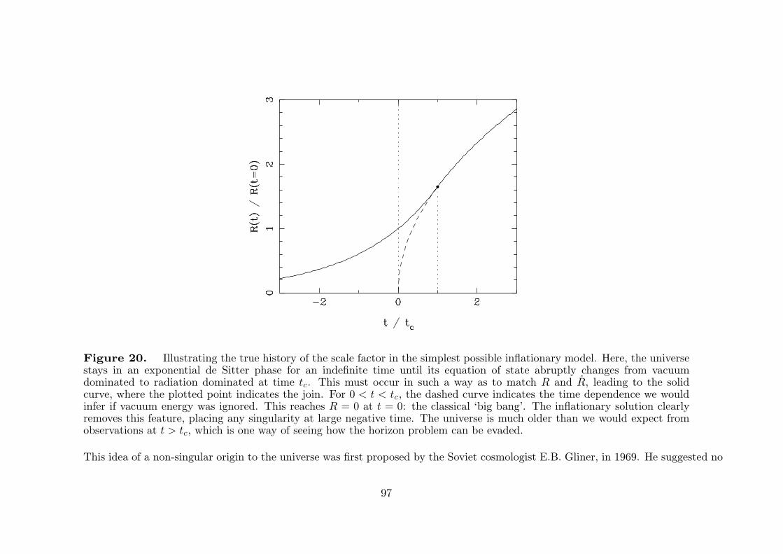
Figure 20. Illustrating the true history of the scale factor in the simplest possible inflationary model. Here, the universestays in an exponential de Sitter phase for an indefinite time until its equation of state abruptly changes from vacuumdominated to radiation dominated at time tc. This must occur in such a way as to match R and R, leading to the solidcurve, where the plotted point indicates the join. For 0 < t < tc, the dashed curve indicates the time dependence we wouldinfer if vacuum energy was ignored. This reaches R = 0 at t = 0: the classical ‘big bang’. The inflationary solution clearlyremoves this feature, placing any singularity at large negative time. The universe is much older than we would expect fromobservations at t > tc, which is one way of seeing how the horizon problem can be evaded.

This idea of a non-singular origin to the universe was first proposed by the Soviet cosmologist E.B. Gliner, in 1969. He suggested no

97

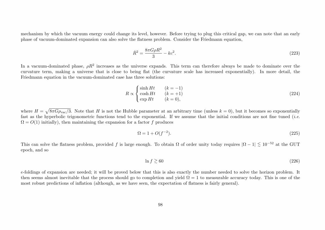
mechanism by which the vacuum energy could change its level, however. Before trying to plug this critical gap, we can note that an earlyphase of vacuum-dominated expansion can also solve the flatness problem. Consider the Friedmann equation,

R2 =8πGρR2

3− kc2. (223)

In a vacuum-dominated phase, ρR2 increases as the universe expands. This term can therefore always be made to dominate over thecurvature term, making a universe that is close to being flat (the curvature scale has increased exponentially). In more detail, theFriedmann equation in the vacuum-dominated case has three solutions:

R ∝⎧⎨⎩sinhHt (k = −1)coshHt (k = +1)expHt (k = 0),

(224)

where H =√8πGρvac/3. Note that H is not the Hubble parameter at an arbitrary time (unless k = 0), but it becomes so exponentially

fast as the hyperbolic trigonometric functions tend to the exponential. If we assume that the initial conditions are not fine tuned (i.e.Ω = O(1) initially), then maintaining the expansion for a factor f produces

Ω = 1 +O(f−2). (225)

This can solve the flatness problem, provided f is large enough. To obtain Ω of order unity today requires |Ω − 1| <∼ 10−52 at the GUTepoch, and so

ln f >∼ 60 (226)

e-foldings of expansion are needed; it will be proved below that this is also exactly the number needed to solve the horizon problem. Itthen seems almost inevitable that the process should go to completion and yield Ω = 1 to measurable accuracy today. This is one of themost robust predictions of inflation (although, as we have seen, the expectation of flatness is fairly general).

98

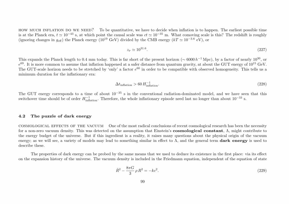
how much inflation do we need? To be quantitative, we have to decide when inflation is to happen. The earliest possible timeis at the Planck era, t � 10−43 s, at which point the causal scale was ct � 10−35 m. What comoving scale is this? The redshift is roughly(ignoring changes in geff) the Planck energy (10

19 GeV) divided by the CMB energy (kT � 10−3.6 eV), or

zP � 1031.6. (227)

This expands the Planck length to 0.4 mm today. This is far short of the present horizon (∼ 6000h−1Mpc), by a factor of nearly 1030, ore69. It is more common to assume that inflation happened at a safer distance from quantum gravity, at about the GUT energy of 1015 GeV.The GUT-scale horizon needs to be stretched by ‘only’ a factor e60 in order to be compatible with observed homogeneity. This tells us aminimum duration for the inflationary era:

Δtinflation > 60H−1inflation. (228)

The GUT energy corresponds to a time of about 10−35 s in the conventional radiation-dominated model, and we have seen that thisswitchover time should be of order H−1

inflation. Therefore, the whole inflationary episode need last no longer than about 10−33 s.

4.2 The puzzle of dark energy

cosmological effects of the vacuum One of the most radical conclusions of recent cosmological research has been the necessityfor a non-zero vacuum density. This was detected on the assumption that Einstein’s cosmological constant, Λ, might contribute tothe energy budget of the universe. But if this ingredient is a reality, it raises many questions about the physical origin of the vacuumenergy; as we will see, a variety of models may lead to something similar in effect to Λ, and the general term dark energy is used todescribe these.

The properties of dark energy can be probed by the same means that we used to deduce its existence in the first place: via its effecton the expansion history of the universe. The vacuum density is included in the Friedmann equation, independent of the equation of state

R2 − 8πG

3ρR2 = −kc2. (229)

99

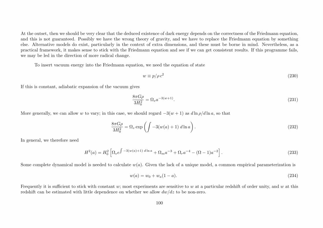
At the outset, then we should be very clear that the deduced existence of dark energy depends on the correctness of the Friedmann equation,and this is not guaranteed. Possibly we have the wrong theory of gravity, and we have to replace the Friedmann equation by somethingelse. Alternative models do exist, particularly in the context of extra dimensions, and these must be borne in mind. Nevertheless, as apractical framework, it makes sense to stick with the Friedmann equation and see if we can get consistent results. If this programme fails,we may be led in the direction of more radical change.

To insert vacuum energy into the Friedmann equation, we need the equation of state

w ≡ p/ρ c2 (230)

If this is constant, adiabatic expansion of the vacuum gives

8πGρ

3H20

= Ωva−3(w+1). (231)

More generally, we can allow w to vary; in this case, we should regard −3(w + 1) as d ln ρ/d ln a, so that

8πGρ

3H20

= Ωv exp

(∫−3(w(a) + 1) d ln a

). (232)

In general, we therefore need

H2(a) = H20

[Ωve

∫−3(w(a)+1) d ln a +Ωma

−3 +Ωra−4 − (Ω− 1)a−2

]. (233)

Some complete dynamical model is needed to calculate w(a). Given the lack of a unique model, a common empirical parameterization is

w(a) = w0 + wa(1− a). (234)

Frequently it is sufficient to stick with constant w; most experiments are sensitive to w at a particular redshift of order unity, and w at thisredshift can be estimated with little dependence on whether we allow dw/dz to be non-zero.

100

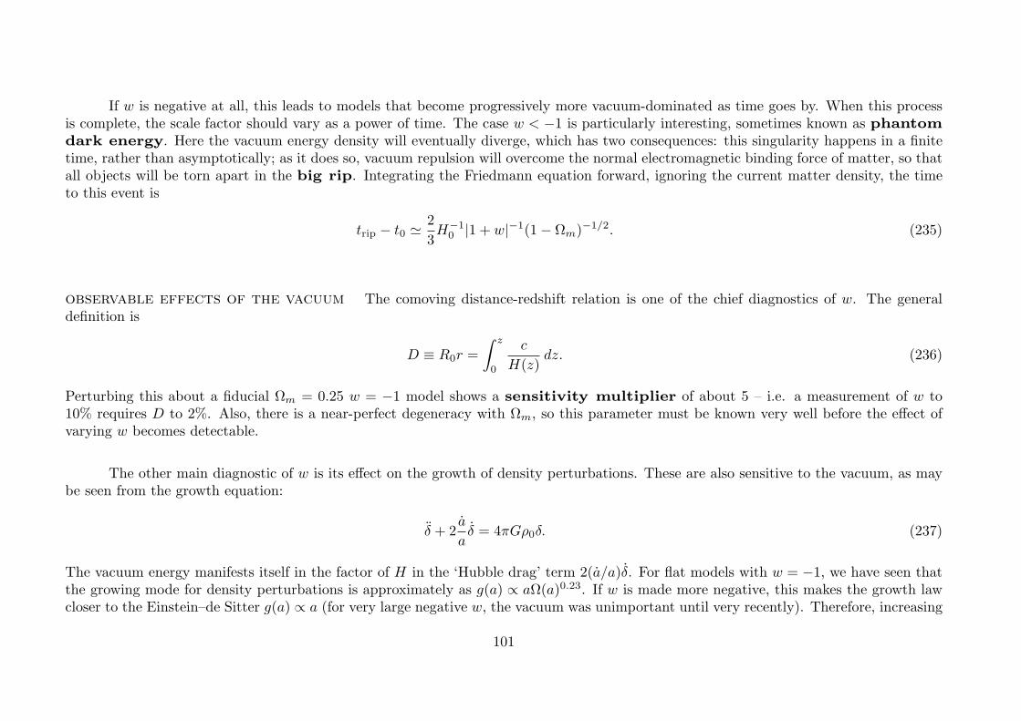
If w is negative at all, this leads to models that become progressively more vacuum-dominated as time goes by. When this processis complete, the scale factor should vary as a power of time. The case w < −1 is particularly interesting, sometimes known as phantomdark energy. Here the vacuum energy density will eventually diverge, which has two consequences: this singularity happens in a finitetime, rather than asymptotically; as it does so, vacuum repulsion will overcome the normal electromagnetic binding force of matter, so thatall objects will be torn apart in the big rip. Integrating the Friedmann equation forward, ignoring the current matter density, the timeto this event is

trip − t0 � 2

3H−1

0 |1 + w|−1(1− Ωm)−1/2. (235)

observable effects of the vacuum The comoving distance-redshift relation is one of the chief diagnostics of w. The generaldefinition is

D ≡ R0r =

∫ z

0

c

H(z)dz. (236)

Perturbing this about a fiducial Ωm = 0.25 w = −1 model shows a sensitivity multiplier of about 5 – i.e. a measurement of w to10% requires D to 2%. Also, there is a near-perfect degeneracy with Ωm, so this parameter must be known very well before the effect ofvarying w becomes detectable.

The other main diagnostic of w is its effect on the growth of density perturbations. These are also sensitive to the vacuum, as maybe seen from the growth equation:

δ + 2a

aδ = 4πGρ0δ. (237)

The vacuum energy manifests itself in the factor of H in the ‘Hubble drag’ term 2(a/a)δ. For flat models with w = −1, we have seen thatthe growing mode for density perturbations is approximately as g(a) ∝ aΩ(a)0.23. If w is made more negative, this makes the growth lawcloser to the Einstein–de Sitter g(a) ∝ a (for very large negative w, the vacuum was unimportant until very recently). Therefore, increasing

101

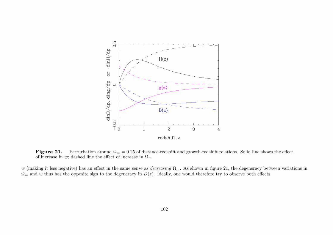
Figure 21. Perturbation around Ωm = 0.25 of distance-redshift and growth-redshift relations. Solid line shows the effectof increase in w; dashed line the effect of increase in Ωm

w (making it less negative) has an effect in the same sense as decreasing Ωm. As shown in figure 21, the degeneracy between variations inΩm and w thus has the opposite sign to the degeneracy in D(z). Ideally, one would therefore try to observe both effects.

102

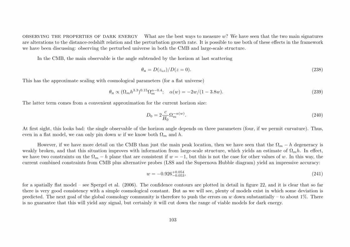
observing the properties of dark energy What are the best ways to measure w? We have seen that the two main signaturesare alterations to the distance-redshift relation and the perturbation growth rate. It is possible to use both of these effects in the frameworkwe have been discussing: observing the perturbed universe in both the CMB and large-scale structure.

In the CMB, the main observable is the angle subtended by the horizon at last scattering

θH = D(zLS)/D(z = 0). (238)

This has the approximate scaling with cosmological parameters (for a flat universe)

θH ∝ (Ωmh3.3)0.15Ωα−0.4

m ; α(w) = −2w/(1− 3.8w). (239)

The latter term comes from a convenient approximation for the current horizon size:

D0 = 2c

H0Ω−α(w)

m . (240)

At first sight, this looks bad: the single observable of the horizon angle depends on three parameters (four, if we permit curvature). Thus,even in a flat model, we can only pin down w if we know both Ωm and h.

However, if we have more detail on the CMB than just the main peak location, then we have seen that the Ωm − h degeneracy isweakly broken, and that this situation improves with information from large-scale structure, which yields an estimate of Ωmh. In effect,we have two constraints on the Ωm − h plane that are consistent if w = −1, but this is not the case for other values of w. In this way, thecurrent combined constraints from CMB plus alternative probes (LSS and the Supernova Hubble diagram) yield an impressive accuracy:

w = −0.926+0.054−0.053, (241)

for a spatially flat model – see Spergel et al. (2006). The confidence contours are plotted in detail in figure 22, and it is clear that so farthere is very good consistency with a simple cosmological constant. But as we will see, plenty of models exist in which some deviation ispredicted. The next goal of the global cosmology community is therefore to push the errors on w down substantially – to about 1%. Thereis no guarantee that this will yield any signal, but certainly it will cut down the range of viable models for dark energy.

103

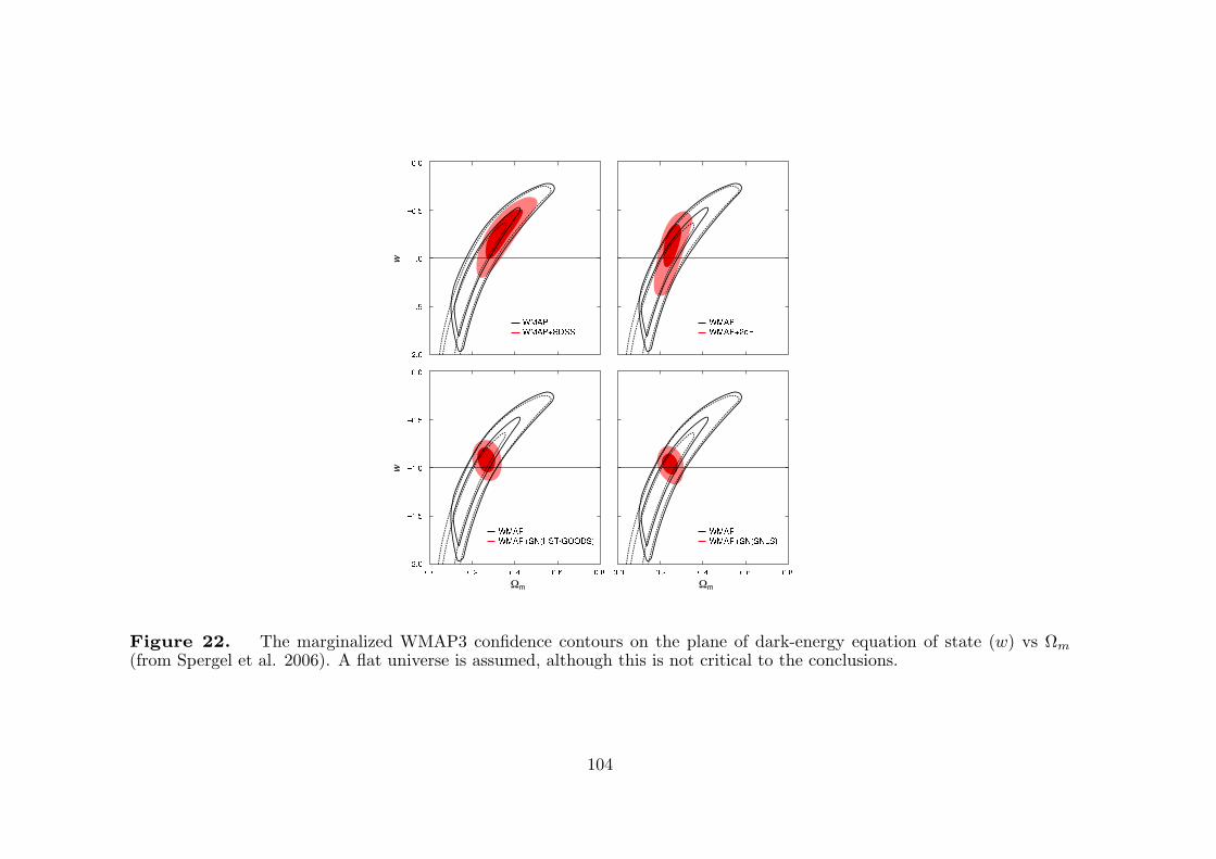
Figure 22. The marginalized WMAP3 confidence contours on the plane of dark-energy equation of state (w) vs Ωm

(from Spergel et al. 2006). A flat universe is assumed, although this is not critical to the conclusions.

104

4.3 The anthropic approach

Whether or not one finds the ‘essence’ approach compelling, there remains one big problem. All the models are constructed using Lagrangianswith a particular zero level. All quintessence potentials tend to zero for large fields, and k-essence models lack a potential altogether. Theyare therefore subject to the classical dilemma of the cosmological constant: adding a pure constant to the Lagrangian has no affect on fielddynamics, but mimics a cosmological constant. With so many possible contributions to this vacuum energy from the zero-point energies ofdifferent fields (if nothing else), it seems contrived to force V (φ) to asymptote to zero without a reason.

This leads us in the direction of anthropic arguments, which are able to limit Λ to some extent: if the universe had become vacuum-dominated at z > 1000, gravitational instability would have been impossible – so that galaxies, stars and observers would not have beenpossible (Weinberg 1989). Indeed, Weinberg made the astonishingly prescient prediction on this basis that a non-zero vacuum densitywould be detected at Ωv of order unity, since there was no reason for it to be much smaller.

many universes At first sight, this argument seems quite appealing, but it rapidly leads us into deep waters. How can we talk aboutchanging Λ? It has the value that it has. We are implicitly invoking an ensemble picture in which there are many universes withdiffering properties. This is a big step (although exciting, if this turns out to be the only way to explain the vacuum level we see). Infact, the idea of an ensemble emerges inevitably from the framework of inflationary cosmology, since the fluctuations in the scalar field canaffect the progress of inflation itself. We have used this idea to look at the changes in when inflation ends – but fluctuations can affectthe field at all stages of its evolution. They can be thought of as adding a random-walk element to the classical rolling of the scalar fielddown the trough defined by V (φ). In cases where φ is too close to the origin for inflation to persist for sufficiently long, it is possible forthe quantum fluctuations to push φ further out – creating further inflation in a self-sustaining process. This is the concept of stochasticeternal inflation due to Linde. Sufficiently far from the origin, the random walk effect of fluctuations becomes more marked and canoverwhelm the classical downhill rolling. This means that some regions of space can inflate for an indefinite time, and a single inflatinguniverse automatically breaks up into different bubbles with their own histories. Some random subset of these eventually random-walkclose enough to the origin that the classical end of inflation can occur, thus creating a set of ‘universes’ each of which can potentially hostobservers.

With this as a starting point, the question now becomes whether we can arrange for the different members of this ensemble tohave different values of Λ. This is easily achieved. Let there be some quintessence field with a very flat potential, so that it is capable of

105

simulating Λ effectively. Quantum fluctuations during inflation can also displace this field, so that each member of the multiverse wouldhave a different Λ.

the distribution of Λ We are now almost in a position to calculate a probability distribution for Λ. First, we have to set someground rules: what will vary and what will be held fixed? We should try to change as little as possible, so we assume that all universeshave the same values for

(1) The Baryon fraction fb = ρb/ρm.

(2) The entropy per particle S = (T/2.73)3/Ωmh2

(3) The horizon-scale inhomogeneity δH � 10−5.

It is far from clear that these minimal assumptions are correct. For example, string theorists have evolved the notion of thelandscape, in which there is no unique form for low-energy particle physics, but instead a large number of possibilities in which numberssuch as the fine-structure constant, neutrino masses etc. are different. From the point of view of understanding Λ, we need there to be atleast 10100 possible states so that at least some have Λ smaller than the natural m4

pdensity by a sufficient factor. The landscape hypothesis

really took off in 2001, when this number was first shown to be about 10500. But to start with, the simplest approach makes sense: if thesimplest forms of anthropic variation can be ruled out, this might be taken as evidence in favour of the landscape picture.

We then take a Bayesian viewpoint to the distribution of Λ given the existence of observers:

P (Λ | Observer) ∝ Pprior(Λ)P (Observer | Λ), (242)

where we need both the prior distribution of Λ between different members of the ensemble and how the chance of getting an observer ismodified by Λ. The latter factor should be proportional to the number of stars, which is generally take to be proportional to the fraction ofthe baryons that are incorporated into nonlinear structures. We can estimate this using the Press-Schechter apparatus to get the collapsefraction into systems of a galaxy-scale mass. The exact definition of this is not very important, since the CDM power spectrum is very flaton small scales: any mass at all close to 1012M� gives similar answers.

106

The more difficult part is the prior distribution of Λ, and a common argument is to say that it has a uniform distribution – whichseems reasonable enough if we are to allow it to have either sign, but know that we will be interested in a very small range near zero. Thisis the startling proposition of the anthropic model: the vacuum density takes large ranges, and in almost all realizations, the values arecomparable in magnitude to the natural scale m4

P; such models are stupendously inimical to life.

We therefore have the simple model

dP (ρv) ∝ fc dρv, (243)

where fc is the collapse fraction into galaxy-scale objects. For large values of Λ, growth ceases at high redshift, and fc is exponentiallysuppressed. But things are less clear-cut if Λ < 0. Here the universe eventually recollapses, and the high density means that the collapsefraction always tends to unity. So why do we not observe Λ < 0? The answer is that we have to cut off the calculation at late stages ofrecollapse: once the universe becomes too hot, star-formation may be affected and in any case there is little time for life to form.

With this proviso, figure 23 shows the posterior distribution of Λ conditional on the existence of observers in the multiverse. Weexpress things in natural units: if we adopt the values Ωv = 0.75 and h = 0.73 for the key cosmological parameters, then

ρv = 7.51× 10−27 kgm−3 =h

c

(Ev

hc

)4

, (244)

where Ev = 2.39 meV is known to a tolerance of about 1 %. Provided we consider recollapse only to a maximum temperature of about 10K, the observed figure is matched well by the anthropic prediction: with this cutoff, most observers will see a positive Λ, and something oforder 10% of observers will see Λ as big as we do, or smaller.

So is the anthropic explanation the correct one? Many people find the hypothesis too radical: why postulate an infinity of universesin order to explain a detail of one of them? Certainly, if an alternative explanation for the ‘why now’ problem existed in the form of e.g. anaturally successful quintessence model, one might tend to prefer that. But so far, there is no such alternative. The longer this situationpersists, the more we will be forced to accept that the universe we see can only be understood by making proper allowance for our role asobservers.

107

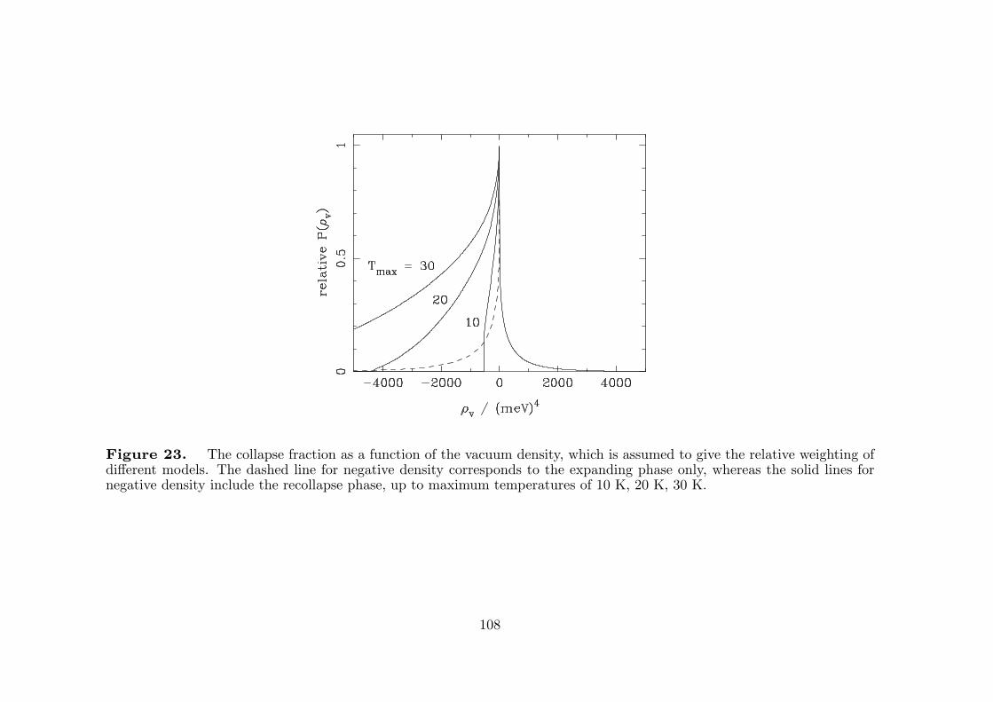
Figure 23. The collapse fraction as a function of the vacuum density, which is assumed to give the relative weighting ofdifferent models. The dashed line for negative density corresponds to the expanding phase only, whereas the solid lines fornegative density include the recollapse phase, up to maximum temperatures of 10 K, 20 K, 30 K.

108

Bibliography

With apologies, these notes do not include a consistent bibliography. The papers referred to above can be located efficiently bysearching on ADS: adswww.harvard.edu/ads abstracts.html

Exercises

Here are some problems that may be useful in testing comprehension of the material in these lectures.

Problem (1)

(a) Starting from the Friedmann equation, show that the Hubble parameter as a function of epoch can be written as

H2(a) = H20

(Ωma

−3 +Ωra−4 +Ωv +Ωka

−2), (245)

defining carefully all terms that appear. Explain why the Ωk term does not represent a contribution to the matter density. How does theequation chance if the vacuum energy is given a constant equation of state w = −1? Show that, provided w < −1/3, the universe willbecome vacuum dominated in the far future.

(b) If w < −1, show from the Friedmann equation that the scale factor diverges at a finite time in the future. If the current matterdensity is neglected in comparison with the vacuum density, show that the time to this event is approximately

t− t0 � 2

3H−1

0 |1 + w|−1Ω−1/2v . (246)

(c) If the vacuum density is negative, prove that the expansion of the universe will always result in a maximum for the scale factor,followed by collapse to a big crunch, provided w < −1/3. For the case of a flat universe containing only matter and vacuum with w = −1,show that the Friedmann equation may be written as a2 = −a2 +1/a with a suitable choice of time unit. Thus derive the exact expressionfor a(t) and hence the time of maximum expansion and the time of the big crunch. The substitution y = a3/2 should be useful.

(d) Write down the integral for the relation between comoving distance and redshift. Discuss the use of this relation at the timeof maximum expansion in the above recollapsing universe, and show that the leading dependence of redshift on distance is quadratic indistance.

109

Problem (2)

(a) Write down the integrals for the relation between cosmological time and redshift, and for the relation between the particle horizonand redshift. Show that the proper size of the particle horizon during the early radiation-dominated era is 2ct, and explain how this distancecan be larger than ct.

(b) Write down the integral for the relation between comoving distance and redshift, and explain the meaning of the terms ‘particlehorizon’ and ‘event horizon’. Give the relation between the current distance to an object at redshift z, the current particle horizon, andthe particle horizon at the time when the light we now receive was emitted.

(c) The North and South Hubble Deep Fields are two small patches that lie in opposite directions on the sky, and which containstatistically identical galaxy populations. Show that, according to the above model for H(a), there are critical redshifts beyond whichpoints in the two Hubble Deep Fields have not established causal contact (a) by the present day; (b) by the time at which the light we nowsee was emitted. Considering the following table of comoving distances for a flat Ωm = 0.25 model, estimate these redshifts.

z D(z)/ h−1Mpc

0.5 13451 23851.5 31782 37953 46905 577510 7051∞ 10666

110

Problem (3)

The equation describing the growth of density fluctuations in a matter-dominated expanding universe is

δ + 2a

aδ = δ

(4πGρm − c2sk2/a2

), (247)

where δ is the fractional density fluctuation, ρ = ρm(1 + δ), ρm is the mean matter density, cs is the speed of sound, and k is comovingwavenumber.

(a) Show that, for a static model, density fluctuations grow exponentially as long as the wavelength is sufficiently large, and explainphysically why this is so.

(b) Derive the solutions to the perturbation equation for a universe of critical density, in the limit of infinitely long wavelength.

(c) At time t = tc, a homogeneous critical-density universe is given a velocity perturbation, such that δ = A. Evaluate the densityperturbation as a function of time following this event.

(d) If the universe contains a homogeneous component in addition to matter that can clump, the perturbation equation still applies– but ρm does not include the homogeneous component. Consider a flat universe that contains a mixture of hot and cold dark matter: forsufficiently small wavelengths, the hot component can be assumed to be uniform, with density parameter Ωh. Show that fluctuations inthe cold component grow as δ ∝ tα, where α = (

√25− 24Ωh − 1)/6.

111