214 Pseudo-Noise and Regenerative Ranging

810-005, Rev. E

DSMS Telecommunications LinkDesign Handbook

1 of 1

214Pseudo-Noise and Regenerative Ranging

NoticeThis module discusses capabilities that have not yet been implemented bythe DSN but have adequate maturity to be considered for spacecraft missionand equipment design. Telecommunications engineers are advised that anycapabilities discussed in this module cannot be committed to except bynegotiation with the Interplanetary Network Directorate (IPN) Plans andCommitments Program Office. < http://deepspace.jpl.nasa.gov/advmiss/>

This page intentionally left blank.

810-005, Rev. E

DSMS Telecommunications Link Design Handbook

1 of 35

214 Pseudo-Noise and Regenerative Ranging

Change 1, Released March 31, 2004

Document Owner: Signature on file at DSMS Library

Approved by: Signature on file at DSMS Library

C. J. Ruggier Date Tracking System Engineer

J. B. Berner Date Telecommunication Service System Development Engineer

Author Signature on file at DSMS Library

Released by: Signature on file at DSMS Library

3/31/04

P. W. Kinman Date

IPN Document Release Date

810-005, Rev. E 214

2

Change Log

Rev Issue Date Affected

Paragraphs Change Summary

– 10/7/2003 All Initial Release

Chg 1 3/31/2004 2.8 Deleted paragraph – duplicate of 2.7

Note to Readers

There are two sets of document histories in the 810-005 document that are reflected in the header at the top of the page. First, the entire document is periodically released as a revision when major changes affect a majority of the modules. For example, this module is part of 810-005, Revision E. Second, the individual modules also change, starting as an initial issue that has no revision letter. When a module is changed, a change letter is appended to the module number on the second line of the header and a summary of the changes is entered in the module’s change log.

810-005, Rev. E 214

3

Contents

Paragraph Page

1. Introduction ....................................................................................................................... 5

1.1 Purpose ..................................................................................................................... 5 1.2 Scope ........................................................................................................................ 5

2. General Information .......................................................................................................... 5

2.1 System Description ................................................................................................. 6 2.2 Parameters Specified for Ranging Operations ......................................................... 7

2.2.1 Range Clock................................................................................................ 8 2.2.2 Pseudo-Noise Signal Structure ................................................................... 8 2.2.3 Integration Time ......................................................................................... 11 2.2.4 Uplink Ranging Modulation Index ............................................................. 12 2.2.5 Tolerance .................................................................................................... 12

2.3 Allocation of Link Power......................................................................................... 12 2.3.1 Uplink ......................................................................................................... 13 2.3.2 Downlink .................................................................................................... 13

2.4 Uplink Spectrum ...................................................................................................... 16 2.5 Range Measurement Performance............................................................................ 19

2.5.1 Coherent Operation..................................................................................... 24 2.5.2 Noncoherent Operation............................................................................... 25

2.6 Range Corrections .................................................................................................... 30 2.6.1 DSS Delay................................................................................................... 31 2.6.2 Z-Correction................................................................................................ 32 2.6.3 Antenna Correction..................................................................................... 32

2.7 Ground Instrumentation Error Contribution ............................................................ 32

References .................................................................................................................................. 35

810-005, Rev. E 214

4

Illustrations

Figure Page

1. The DSN Ranging System Architecture ........................................................................ 7

2. Pseudo-Noise Ranging Signal for Example Composite Code ....................................... 12

3. Uplink Spectrum for the Ranging Signal of Paragraph 2.2.2.1...................................... 18

4. Uplink Ranging Modulation Filter Frequency Response............................................... 20

5. Range Measurement Error for the Composite Code of Paragraph 2.2.2.1..................... 25

6. Probability of Acquisition for the Composite Code of Paragraph 2.2.2.1 ..................... 26

7. Range Measurement Error for the Composite Code of Paragraph 2.2.2.2..................... 27

8. Probability of Acquisition for the Composite Code of Paragraph 2.2.2.2 ..................... 28

9. DSN Range Measurement .............................................................................................. 31

10. Typical DSS Delay Calibration...................................................................................... 33

Tables

Tables Page

1. Component PN Codes Regenerative Ranging Example ................................................ 9

2. Component PN Codes Turn-around Ranging Example ................................................. 10

3. Definition of a(.) and b(.) ............................................................................................. 13

4. Cross-Correlation Factors, Composite Code of Paragraph 2.2.2.1 ................................ 21

5. Cross-Correlation Factors, Composite Code of Paragraph 2.2.2.2 ................................ 21

6. Required ��( )� ◊ � ◊ ��

(in decibels) for Given ln and Pn ............................ 24

7. Ground Instrumentation Range Error for NSP Era Ranging System............................. 34

810-005, Rev. E 214

5

1. Introduction

1.1 Purpose

This module describes the capabilities and expected performance of the DSN when supporting pseudo-noise ranging. These capabilities are being implemented within the 70-m, the 34-m High Efficiency (HEF), and the 34-m Beam Waveguide (BWG) subnets. Performance depends on whether the spacecraft transponder uses a turn-around (non-regenerative) ranging channel or a regenerative ranging channel. Performance parameters are provided for both cases.

1.2 Scope

The material contained in this module covers the pseudo-noise ranging system that may be utilized by both near-Earth and deep space missions. This document describes those parameters and operational considerations that are independent of the particular antenna being used to provide the telecommunications link. For antenna-dependent parameters, refer to the appropriate telecommunications interface module, modules 101, 102, 103, and 104 of this handbook. Other ranging schemes employed by the DSN include sequential ranging, described in module 203, and the tone ranging system, described in module 204.

An overview of the ranging system is given in Paragraph 2.1. The parameters to be specified for ranging operations are explained in Paragraph 2.2. The distribution of link power is characterized in Paragraph 2.3. The spectrum of an uplink carrier modulated by a pseudo-noise ranging signal is discussed in Paragraph 2.4. The performance of non-regenerative and regenerative ranging is summarized in Paragraph 2.5. The case of noncoherent ranging is also discussed there. Paragraph 2.6 provides the corrections required to determine the actual range to a spacecraft. Error contributions of the ground instrumentation are discussed in Paragraph 2.7.

2. General Information

The DSN ranging system provides a ranging signal for measuring the round-trip light time (RTLT) between a Deep Space Station (DSS) and a spacecraft. The ranging signal of interest in this module is a logical combination of a range clock and several pseudo-random noise (PN) codes. The DSS transmits an uplink carrier that has been phase modulated by this ranging signal. The modulated uplink carrier is received and processed by the spacecraft transponder. The ranging channel of the transponder may be either a relatively simple turn-around (non-regenerative) channel or a regenerative channel. In either case, the downlink carrier is phase modulated by a close likeness of the uplink ranging signal. Back at the DSS, the downlink carrier is demodulated. The received ranging signal is correlated with a local model of the range clock and each of the individual PN codes that is a component of the signal. The ranging process can resolve range to a value that is modulo the period of the ranging code. This modulo value is referred to at the range code ambiguity.

810-005, Rev. E 214

6

For coherent operation, the downlink range clock is coherently related to the downlink carrier. The proper frequency to use in generating a local model of the ranging signal is calculated from the measured downlink carrier frequency. Non-coherent operation is discussed in paragraph 2.5.2.

2.1 System Description

The architecture for the DSN ranging system is shown in Figure 1. It consists of a front end portion, an uplink portion, and a downlink portion. The front-end portion consists of the microwave components, including a low-noise amplifier (LNA) and the antenna. The uplink portion includes the Uplink Ranging Assembly (URA), an exciter, the transmitter, and the controller, referred to as the Uplink Processor Assembly (UPA). The downlink portion includes the RF-to-IF Downconverter (RID), the IF-to-Digital Converter (IDC), the Receiver and Ranging Processor (RRP) and the Downlink Channel Controller (DCC). The Downlink Telemetry and Tracking Subsystem (DTT) and the Uplink Subsystem (UPL) provide the essential functional capability for DSN ranging.

The URA uplink ranging function is controlled by the UPL. The RRP downlink ranging function is controlled by the DTT. Each subsystem measures the range phase and sends the measurements to the Tracking Data Delivery Subsystem (TDDS) via the Reliable Network Service (RNS). The URA generates the uplink ranging signal and measures its phase before the signal passes to the exciter modulator. The range signal is phase modulated onto the carrier and transmitted to the spacecraft. The spacecraft turns around the signal, sending it back to the DSN receiver.

The amplified downlink signal from the antenna is downconverted by the RID (located on the antenna) and fed to an intermediate frequency (IF) distribution assembly in the control room. The IF is fed to one or more Downlink Channel Processing Cabinets (DCPC) as required. Each DCPC is equipped with a single channel, which includes a single IDC and RRP. For spacecraft with multiple channels (for example, S-band and X-band), or for multiple spacecraft within a single antenna beamwidth, multiple DCPCs will be assigned to that antenna.

After processing, the downlink range phase data are delivered to the TDDS by the Downlink Channel Controller (DCC), via the station RNS and a similar function at JPL. The TDDS combines the uplink and downlink phase information to produce range data, formats the ranging data and passes it along with the uplink and downlink phase information to the Navigation subsystem (NAV). Subsequently, the NAV provides the ranging data to projects.

Range data are delivered to users in the form of Range Units (RU). Range units are defined, for historical reasons related to hardware design, as two cycles of the S-band uplink frequency (the only frequency band that was in use when the definition was established). As 2 cycles of a 2 GHz frequency occur in a nanosecond, RUs are often described as being approximately 1 ns. They are, in fact, dimensionless but can be converted to physical units of seconds by the following equation.

810-005, Rev. E 214

7

Figure 1. The DSN Ranging System Architecture

��

�� =

�¥ ��

��

��

◊ �¥ ��

��

Ï

Ì Ô Ô

Ó Ô Ô

(1)

where RU is the reported number of range units and ƒS is the frequency of the S-band uplink carrier or ƒX is the frequency of the X-band uplink carrier in MHz. The DSN does not presently support ranging using a Ka-band uplink carrier.

For example, if an X-Band uplink of 7,160 MHz is being used and suppose the measurement obtained is 6,500,000 RU, then the equivalent RTLT delay is 6,153,467 ns, and the one-way distance (multiplying by c/2) is about 922,381.50 m.

2.2 Parameters Specified for Ranging Operations

The following paragraphs present the parameters that are required in ranging operations.

810-005, Rev. E 214

8

2.2.1 Range Clock

The range clock is a periodic signal, usually a sinewave. It represents the most visible component of the ranging signal for pseudo-noise ranging operation. The range clock on the uplink is coherently related to the uplink carrier. The frequency ƒRC of this range clock is related to that of the uplink carrier by

��

�� =

�

�� ◊ ��¥ ��

��

¥ �

�� ◊ ��¥ ��

Ï

Ì Ô Ô

Ó Ô Ô

(2)

where ƒS is the frequency of an S-band uplink carrier and ƒX is the frequency of an X-band uplink carrier. The integer k is limited to 1��k �� !�"#�$�!!��" ��%�� $��$��frequency is near 1 MHz, corresponding to k = 4. The exact value of fRC depends on the channel assignment and on whether there is Doppler compensation on the uplink. A k of 5 results in a range clock frequency of about 500 kHz, a k of 6 results in a range clock frequency of about 250 kHz, etc.

In the interest of uplink spectrum conservation, all range clocks corresponding to k ��&��% �"�� ' "��(�� ' %��%�� $��$�"�$�%% "��#��k )��!�� squarewaves. The range measurement error due to thermal noise is smaller for higher range clock frequencies (i.e., lower component numbers), so it is expected that most missions will use sinewave range clocks.

2.2.2 Pseudo-Noise Signal Structure

The pseudo-noise ranging signal is based on a composite code. The composite code, in turn, is built out of component PN codes. These codes are generated in software (References 1 and 2), and there is a great deal of flexibility in the design of these codes. Two example composite codes are described below. The first is suitable for regenerative ranging, and the second is a better choice for turn-around (non-regenerative) ranging.

2.2.2.1 Example Composite Code, Regenerative Ranging

The idea of building a composite code out of component PN codes is illustrated here with an example. This example design is built from 6 component PN codes and is suitable for regenerative ranging (References 3 and 4). The length of the nth component code is ln, for 1��n ��&�� # "��% *�l1 = 2, l2 = 7, l3 = 11, l4 = 15, l5 = 19, and l6 = 23. The first PN code is a trivial 2-chip sequence representing the range clock. The nth component code is denoted Cn(i), where i represents a discrete-time index, 0 ��i < ln. The 6 component codes are given in Table 1. The proper order of each of these component codes is determined by reading the chips in each row from left to right. (So, for example, the first three chips of C3 are all 1’s and the final chip is a 0.)

810-005, Rev. E 214

9

Table 1. Component PN Codes Regenerative Ranging Example

Code Bit Sequence

C1 1, 0

C2 1, 1, 1, 0, 0, 1, 0

C3 1, 1, 1, 0, 0, 0, 1, 0, 1, 1, 0

C4 1, 1, 1, 1, 0, 0, 0, 1, 0, 0, 1, 1, 0, 1, 0

C5 1, 1, 1, 1, 0, 1, 0, 1, 0, 0, 0, 0, 1, 1, 0, 1, 1, 0, 0

C6 1, 1, 1, 1, 1, 0, 1, 0, 1, 1, 0, 0, 1, 1, 0, 0, 1, 0, 1, 0, 0, 0, 0

For each code Cn(i), a periodic code C¢n(i) of period ln is formed by endless repetition. That is,

¢ �� ( )= � �!�� l�( ) (3)

The composite code is

�� + �( )= ¢ �� ( )» ¢ �� ( )« ¢ �� ( )« ¢ �� ( )« ¢ �� ( )« ¢ �� ( )[ ] (4)

where » and « are the logical OR and logical AND operators, respectively. Since the component PN code lengths are relatively prime, the period (in chips) L of the composite code is the product of the component PN code lengths. That is,

Seq(i + L) = Seq(i) (5)

where

�� = l� =��$ ��"

�=�

&

’ (6)

Using relatively prime numbers (that is, integers that share no common divisors except 1) gives a large L for relatively small component PN code lengths. This is important because a large L is necessary for resolution of the range ambiguity, yet small ln are needed for a practical implementation of the correlators at the receiver. The ambiguity of this code when using a range clock of approximately 1 MHz is

�� = $ ◊

� �� ª ��,�&&��!� (7)

810-005, Rev. E 214

10

An important property of the composite code is that it approximates a sequence of period 2 chips. As seen in Equation (4), the composite code equals C¢n(i), the first component with a period of 2 chips, most of the time. The effect of the other 5 component PN codes is to invert a small fraction (1/32) of the logical 0’s in C¢n(i). The resulting pseudo-noise ranging signal approximates a range clock with a frequency equal to one-half the chip rate, and most of this signal’s power is at the range clock frequency. This is desirable, since the precision of the range measurement is set by a correlation against a local model of the range clock. The occasional chip inversion is necessary to resolve the range ambiguity, but for this purpose the inversions need not be frequent.

2.2.2.2 Example Composite Code, Turn-around Ranging

This example design is built from 5 component PN codes and is a good choice for turn-around ranging (Reference 5). The length of the nth component code is ��l�

, for 1��n ��,�� lengths are: ��l� = �� l� = �� l� =�� l� =�,� �� l� =�� The numbers ��l�

(1��n ��,-��% �relatively prime. The nth component code is denoted Cn(i), 0��i <��l�

. The 5 component codes are given in Table 2. (These five component codes are the same as the first five codes of Table 1.) The proper order of each of these component codes is determined by reading the chips in each row from left to right. (So, for example, the first three chips of C3 are all 1’s and the final chip is a 0.)

Table 2. Component PN Codes Turn-around Ranging Example

Code Bit Sequence

C1 1, 0

C2 1, 1, 1, 0, 0, 1, 0

C3 1, 1, 1, 0, 0, 0, 1, 0, 1, 1, 0

C4 1, 1, 1, 1, 0, 0, 0, 1, 0, 0, 1, 1, 0, 1, 0

C5 1, 1, 1, 1, 0, 1, 0, 1, 0, 0, 0, 0, 1, 1, 0, 1, 1, 0, 0

For each code Cn(i), a periodic code C ¢n(i) of period ��l� is formed by endless

repetition. That is,

C ¢n(i) = Cn(i mod ��l�) (8)

810-005, Rev. E 214

11

Each chip in the composite code is determined as a majority vote of the component codes,

�� + �( )=

�� ¢ �� ( )+ ¢ �� ( )+ ¢ �� ( )+ ¢ �� ( )+ ¢ �� ( )≥ .�� # %��"

Ï Ì Ô

Ó Ô (9)

Since the component PN code lengths are relatively prime, the period (in chips) L of the composite code is the product of the component PN code lengths. That is,

Seq(i + L) = Seq(i) (10)

where

�� = l� = �.��$ ��"

�=�

,

’ (11)

The ambiguity of this code when using a range clock of approximately 1 MHz is

�� = $ ◊

� �� ª �.��!� (12)

2.2.2.3 General Limits on Code Design

The composite codes of Paragraphs 2.2.2.1 and 2.2.2.2 are but examples. There are a large number of composite codes that would work well for range measurement. There are, however, some general limits on code design placed by the current DSN implementation. There can be, at most, 6 component codes. The length of any component code may not exceed 64 chips and the overall PN pattern cannot exceed 8,333,608 chips. The chip rate equals twice the range clock frequency, so the limits on range clock frequency given in Paragraph 2.2.1 must be considered.

2.2.2.4 Conversion of Composite Code to Pseudo-Noise Ranging Signal

The pseudo-noise ranging signal is created from the composite code by translating each logical 1 of the composite code into a positive half-cycle of a sinewave and each logical 0 into a negative half-cycle of a sinewave. (However, when the range clock frequency is 125 kHz or less, the half-cycles may be from a squarewave, rather than a sinewave.)

For example, the ranging signal created from the composite code of Paragraph 2.2.2.1 would look as shown in Figure 2. The parameter T represents the chip period, so only the first 8 chips are represented in Figure 2. The range clock frequency equals

�� ( ).

2.2.3 Integration Time

The integration time T should be large enough that the probability of range measurement acquisition is close to 1.0 and the range error due to downlink thermal noise is small (see Paragraph 2.5). With noncoherent ranging, the presence of a frequency mismatch between the received ranging signal and the local model means that there is also reason to keep T relatively small, so that an optimum T should be carefully chosen for noncoherent ranging.

810-005, Rev. E 214

12

Figure 2. Pseudo-Noise Ranging Signal for Example Composite Code

2.2.4 Uplink Ranging Modulation Index

The uplink ranging modulation index is chosen to get a suitable distribution of power among the ranging and command sidebands and the residual carrier on the uplink (see Paragraph 2.3). With turn-around (non-regenerative) ranging, the uplink ranging modulation index also affects the distribution of power on the downlink carrier.

2.2.5 Tolerance

Tolerance is used to set the acceptable limit of the figure of merit (FOM) which is an estimate of the goodness of an acquisition based on the downlink PR/N0 measurement (see Paragraph 2.5).

Tolerance may be selected over the range of 0.0% to 100.0%. As an example, if the tolerance is set to 0.0%, all range acquisitions will be declared valid. Alternately, if the tolerance is set to 100.0%, all range acquisitions will be declared invalid. A typical value set for tolerance is 99.9%. This value will flag acquisitions that have a 99.9% or better chance of being good as valid, and the rest as invalid.

An acquisition is declared valid or invalid depending upon the following criteria:

FOM ) Tolerance results in Acquisition declared valid

FOM < Tolerance results in Acquisition declared invalid.

2.3 Allocation of Link Power

The equations governing the allocation of power on uplink and downlink depend on whether the range clock is sinewave or squarewave. Most often, the range clock will be sinewave; but for the sake of completeness, both cases are considered here. In order to achieve economy of expression, it is advantageous to introduce the functional definitions of Table 3.

Bessel functions of the first kind of order 0 and 1 are denoted J0(.). and J1(.).

810-005, Rev. E 214

13

Table 3. Definition of a(.) and b(.)

Range Clock Command a y( ) b y( )

sinewave sinewave subcarrier ��

/� �y( ) �� /� �y( )

squarewave squarewave subcarrier or

direct modulation ��$�" y( )

��"�� y( )

2.3.1 Uplink

The equations of this paragraph apply to simultaneous ranging and command using a pseudo-noise ranging signal (with sinewave or squarewave range clock) and either a command subcarrier (sinewave or squarewave) or direct command to the uplink carrier. The carrier suppression is

��

� ��

= a � f�( )◊a � f�( ) (13)

The ratio of available ranging signal power to total power is

��

��

= b � f�( )◊a � f�( ) (14)

The ratio of available command (data) signal power to total power is

��

��

= b� f�( )◊a � f�( ) (15)

In these equations, fr is the uplink ranging modulation index in radians rms and fc is the

command modulation index in radians rms. If no command is present, fc = 0, ��a f�( )=�, and the

factor representing command modulation in Equations (13) and (14) is simply ignored. Equation (15) does not apply as

��f�� b f�( )�� =�.

2.3.2 Downlink

The equations for power allocation on the downlink depend on whether the spacecraft transponder has a turn-around (non-regenerative) ranging channel or a regenerative ranging channel.

810-005, Rev. E 214

14

2.3.2.1 Turn-Around (Non-Regenerative) Ranging

A turn-around ranging channel demodulates the uplink carrier, filters and amplifies the baseband signal using automatic gain control, and then remodulates this signal unto the downlink carrier. The automatic gain control serves the important purpose of ensuring that the downlink carrier suppression is approximately constant, independent of received uplink signal level. A typical bandwidth for this turn-around channel is 1.5 MHz – wide enough to pass a 1 MHz ranging clock. Unfortunately, substantial thermal noise from the uplink also passes through this channel. In many deep space scenarios, the thermal noise dominates over the ranging signal in this turn-around channel. Moreover, command signal from the uplink may pass through the channel. In general, then, noise and command signal as well as the desired ranging signal are modulated on the downlink whenever the ranging channel is active. A proper analysis must account for all significant contributors (Reference 6).

The carrier suppression is

��

��

= a � q�( )◊a � q�( )◊ �-q��

◊ $�"� q�( ) (16)


��

��

= b � q�( )◊a � q�( )◊ �-q��

◊ $�"� q�( ) (17)

The ratio of available telemetry (data) signal power to total power is

��

��

= a � q�( )◊a � q�( )◊ �-q��

◊ "�� q�( ) (18)

In these equations, qr is the effective downlink ranging signal modulation index in radians rms,

qc is the effective downlink feedthrough command signal modulation index in radians rms, qn is

the effective noise modulation index in radians rms, and qt is the telemetry modulation index. If command is absent (or if, as often happens in deep space, the feedthrough command signal is

small enough to be safely ignored), qc = 0 and ��a � q

�( )=�, so the factor representing command

modulation in Equations (16), (17) and (18) is simply ignored.

In these equations, it has been assumed that the telemetry signal is binary valued (unshaped bits with squarewave subcarrier or unshaped bits directed modulating the carrier). If the telemetry subcarrier is sinewave, on the other hand, then the factor cos2(qt) of Equations (16)

and (17) must be replaced by ��/�

��q

�( ) and the factor sin2(qt) of Equation (18) must be

replaced by ��/�

��q

�( ), where qt is the telemetry modulation index in radians rms.

810-005, Rev. E 214

15

It is important to understand that the modulation indices qr, qc, and qn are effective

modulation indices. In general, none of them equal the design value qd of the downlink ranging modulation index (also with units radians rms). In fact, the automatic gain control circuit in the turn-around ranging channel enforces the following constraint.

��q�� + q�

� + q�� = q�

� (19)

In other words, the total power in the turn-around ranging channel, which equals the ranging signal power plus the feedthrough command signal power plus the noise power in the channel bandwidth, equals a constant value. The effective downlink modulation indices are given by

��q� = q� ◊ L ◊b f�( )◊a f�( ) (20)

��q� = q� ◊ L ◊a f�( )◊ b f�( ) (21)

��q� = q� ◊ L ◊s� (22)

where, as before, fr is the uplink ranging modulation index in radians rms and fc is the uplink

command modulation index in radians rms. The square of su is given by

��

s�� = �� ◊

��

Ê

Ë Á Á

ˆ

¯ ˜ ˜

-�

(23)

where BR is the turn-around ranging channel (noise-equivalent) bandwidth and ��

is the

uplink total signal power to noise spectral density ratio. The normalization factor L is given by

��

L = �

b � f�( )a � f

�( )+ b � f�( )a � f

�( )+ s�

�

(24)

2.3.2.2 Regenerative Ranging

A regenerative ranging channel demodulates the uplink carrier, tracks the ranging clock, detects the ranging data, and modulates a ranging signal on the downlink that can be assumed to be free of thermal noise and command feedthrough. For the purpose of calculating the distribution of power in the downlink in the case of regenerative ranging, the following equations, based on this assumption, may be used. There will, in general, be phase jitter on the downlink ranging signal that is caused by uplink thermal noise and this jitter is an error source for the two-way range measurement. This error is considered in Paragraph 2.5.

The carrier suppression is

��

� ��

= a � q�( )◊ $�"� q�( ) (25)

810-005, Rev. E 214

16


��

��

= b � q�( )◊ $�"� q�( ) (26)

The ratio of available telemetry (data) signal power to total power is

��

��

= a � q�( )◊ "�� q�( ) (27)

In these equations, qd is the design value of the downlink ranging modulation index in radians

rms, and qt is the telemetry modulation index.

In Equations (25), (26), and (27), it has been assumed that the telemetry signal is binary valued (unshaped bits with squarewave subcarrier or unshaped bits directed modulating the carrier). If the telemetry subcarrier is sinewave, on the other hand, then the factor ( )2cos tq

of Equations (25) and (26) must be replaced by ��/�

��q

�( ) and the factor sin2(qt) of Equation

(27) must be replaced by ��/�

��q

�( ), where qt is the telemetry modulation index in radians rms.

2.4 Uplink Spectrum

The spectrum of the uplink carrier is of some concern because of the very large transmitter powers used on the uplink for deep space missions. A mathematical model for this spectrum is given here for the case of a sinewave range clock and no command.

A pseudo-noise ranging signal is periodic, so its spectrum consists of discrete spectral lines. The spectrum of an uplink carrier that has been phase modulated by only a pseudo-noise ranging signal also consists of discrete spectral lines.

The composite code is Boolean, but the ranging signal is bipolar. A bipolar version of the composite code is needed for an analysis of the spectrum.

�� ( )= -�+ � ◊ �� ( ) (28)

where Seq(i) is the Boolean composite code and i = 0, 1, 2, º is a discrete-time index. In this way, a logical 1 is translated into +1 and a logical 0 is translated into –1. A bipolar version of the range clock is

�� ( )= -�+ � ◊ ¢ �� ( ) (29)

where ��

¢ �� ( )is the Boolean range clock. It should be noted that b1(i) = ±1. Most of the time, the

composite code matches the range clock. A discrepancy signal is defined by

�� ( )= �� ( )◊ � �( ) (30)

810-005, Rev. E 214

17

d(i) equals +1 when the range clock and the composite code agree, which is most of the time. When the range clock and the composite code disagree, d(i) equals –1. The pseudo-noise ranging signal may be mathematically modeled as d(i) sin(pt/T) for the time interval iT ��t < (i + 1)T where T is the chip period. In words, the pseudo-noise ranging signal is a sinewave (range clock) of frequency 1/(2T) except that there is an occasional inversion of a half-cycle. When this signal phase modulates the uplink carrier with modulation index fr (radians rms), the fractional power in each discrete spectral line is given by

��

��

= ��

=0%�$#��%��#�#�� %��#

��"$% # �"� $#%�� # �0% +� �$

�� + ��

Ï

Ì

Ô Ô

Ó

Ô Ô

(31)

where PT is the total uplink power, fc is the uplink carrier frequency, L is the period in chips of the composite code, k is an integer harmonic number, and Xk is given by

�� = �

/� �f�� ( )( )"��$ �

�- �

Ê

Ë Á

ˆ

¯ ˜ 1� �p � + �

�

Ê

Ë Á

ˆ

¯ ˜ � - ��

Ê

Ë Á

ˆ

¯ ˜

È

Î Í

˘

˚ ˙

�=-•

•

Â�=�

-�

Â (32)

where Jm(.) is the Bessel function of the first kind of order m, and

��"��$ �( )=

"�� p�( )p�

(33)

Equation (32) may be evaluated numerically. The values of the Bessel functions decrease very rapidly with increasing

�� , so in practice it is possible to get good accuracy while including only

a few terms from the sum over the integer m. In evaluating Equation (32), the following identity is useful.

��

/-� �( )=/� �( )� �� ' �-/� �( )� ��

Ï Ì Ô

Ó Ô �� (34)

There is a symmetrical power distribution about the carrier. So for every discrete

spectral line at�� + �

�, whose power is given by Equation (31), there is also a discrete spectral

line at �� - �

� with the same power.

Figure 3 illustrates the uplink spectrum for a sinewave range clock with the example composite code of Paragraph 2.2.2.1 and a modulation index fr = 0.2 rad rms. The tallest spectral line is the residual carrier with a carrier suppression of –0.2 dB. The next tallest

810-005, Rev. E 214

18

Figure 3. Uplink Spectrum for the Ranging Signal of Paragraph 2.2.2.1

810-005, Rev. E 214

19

spectral lines are located at fC – fRC and fC + fRC, where fRC is the range clock frequency; these spectral lines each have a power of –17.5 dB relative to PT, which was found by using k = L/2 in Equation (31). At each of the frequencies fC – 2fRC and fC + 2fRC there is a power of –39.7 dB relative to PT (found with k = L). The smaller spectral lines that lie between fC – 2fRC and fC + 2fRC are due to the occasional inversions of half-cycles as represented by d(i).

The representation of the uplink spectrum in the above analysis is approximate. If more accurate results are required, it is necessary to take into account the presence of the uplink ranging filter that filters the ranging signal going to the modulator. The main purpose of this filter is to attenuate a 16 MHz spurious signal that arises from the processing rate used to generate the ranging signal. The filter has the frequency response shown in Figure 4 and is inserted between the URA and the exciter. This figure cannot be used directly to estimate the attenuation of ranging harmonics due to the non-linear transfer functions of the modulation process and fluctuations in the amplitude response within the filter passband.

If the insertion loss were perfectly constant over the passband of the uplink ranging signal, the analysis of the uplink spectrum presented above would stand without correction. However, there is, in general, some small variation of the insertion loss within the passband of the desired ranging signal. A more accurate determination of the uplink spectrum, one that takes the variation in the filter insertion loss and variations of the exciter phase modulator transfer function into account, would probably have to be performed by simulation.

2.5 Range Measurement Performance

Thermal noise introduces an error to range measurement and also occasionally causes a range measurement to fail altogether. The error enters when the received ranging signal is correlated against a local model of the range clock. The failure to acquire a range measurement has its roots in the correlations of the received ranging signal against local models of all other PN codes (i.e., all PN codes except the one corresponding to the range clock) that make up the composite code. The probability that a range measurement does not fail is called the probability of acquisition. Both the error due to thermal noise in the range clock correlation and the probability of acquisition, which is less than 1.0 due to thermal noise in the other correlations, are characterized here.

Before characterizing the range measurement performance, it is first necessary to define the following terms. The composite code, treated as a bipolar signal, is

�� ( )= -�+ � ◊ � + �( ) (35)

where Seq(i) is the Boolean composite code and i = 0,1,2º is a discrete-time index. The PN codes that make up the composite code, treated as bipolar signals, are

�� ( )= -�+ � ◊ ¢ �� ( ) (36)

810-005, Rev. E 214

20

Figure 4. Uplink Ranging Modulation Filter Frequency Response

810-005, Rev. E 214

21

where the C¢n(i) are the Boolean PN codes. It should be noted that s(i) = ±1 and bn(i) = ±1. The cross-correlation (with zero delay) factors Rn are defined by

�� = �

� �( )�� ( )

�=�

-�

Â (37)

where L is the period (in chips) of the composite code. For the example composite code of Paragraph 2.2.2.1, the cross-correlation factors are given in Table 4. For the example composite code of Paragraph 2.2.2.2, the cross-correlation factors are given in Table 5.

Table 4. Cross-Correlation Factors, Composite Code of Paragraph 2.2.2.1

n ln Rn

1 2 0.9544

2 7 0.0456

3 11 0.0456

4 15 0.0456

5 19 0.0456

6 23 0.0456

Table 5. Cross-Correlation Factors, Composite Code of Paragraph 2.2.2.2

n ln Rn

1 2 0.3695

2 7 0.3845

3 11 0.3814

4 15 0.3790

5 19 0.3774

The standard deviation of range measurement error s, in meters rms (one way), due to downlink thermal noise is given by

810-005, Rev. E 214

22

��

s =

$

¶� ◊ �� ◊ �� ◊ .�p � ◊� ◊ ��

Ê Ë Á ˆ

¯ ˜ � "�� ' �%�� $��$�

$

¶� ◊ �� ◊ �� ◊ �,& ◊ � ◊ ��

Ê Ë Á ˆ

¯ ˜ � "+��% ��' �%�� $��$�

Ï

Ì

Ô Ô Ô

Ó

Ô Ô Ô

meters rms (38)

where

c = speed of electromagnetic waves in vacuum

Ac = fractional loss of correlation amplitude due to frequency mismatch (Ac ��-��see paragraphs 2.5.1 and 2.5.2

R1 = cross-correlation factor for the correlation against the range clock, see Tables 4 and 5

T = range measurement integration time

¶RC = frequency of the range clock

�� is given by

��

��

= ��

◊ ��

(39)

where

��

��

is the downlink total signal to noise spectral density ratio

and where �� is the ratio of downlink ranging signal power to total power as given by Equation (17) for turn-around (non-regenerative) ranging or as given by Equation (26) for regenerative ranging. In the case of turn-around ranging, uplink thermal noise has an effect on measurement error through its effect on PR/PT.

In the case of regenerative ranging, uplink thermal noise leads to phase jitter on the regenerated ranging signal. This phase jitter arises in the tracking loop that is part of the regeneration signal processing (Reference 3). This tracking jitter is a potential error source for the two-way range measurement. The standard deviation ��s� of range measurement error

(meters rms, one way) for this error source is given by

��

s� � = ��

��

� �

(40)

810-005, Rev. E 214

23

where BRC is the bandwidth of the loop that tracks the uplink ranging signal and ��

is

the uplink signal power to noise spectral density ratio. This error only applies in the case of regenerative ranging.

The probability of acquisition is, for the case of N components, given by

��$+ = ��

�=�

�

’ (41)

where Pn is the probability of acquiring the nth code component (2 ��n ��N),

��

�� = �

p�-��

�+ %0 � + �� ◊ �� ( )( )�

Ê

Ë

Á Á Á

ˆ

¯

˜ ˜ ˜

l�-�

��-•

•

Ú (42)

where ln and Rn are the code length (in chips) and cross-correlation factor for the nth component

and where erf(.) is the error function

%02 � - = �

p�-�

�

��

�

Ú (43)

Equations (38) and (42) are based on the assumption that the local model of the range clock has a wave shape that matches that of the received range clock. In other words, when the downlink range clock is sinewave, the local model of the range clock used in the correlation is assumed likewise to be sinewave; and when the downlink range clock is squarewave, the local model of the range clock used in the correlation is assumed likewise to be squarewave.

Table 6 lists required values for ��( )� ◊ � ◊ ��

(in decibels) as a function

of ln (the code length) and Pn (the probability of acquiring the nth code component). This table is based on Equation (42). Results are listed in this table for the most common component code lengths. Here is an example of how this table can be used. Suppose the desired Pn for a component code of length 19 is 0.95. Then, log (0.95) = –0.022. From Table 6, the decibel values 7.9 dB and 8.5 dB are found for log(Pn) = –0.030 and log(Pn) = –0.020, respectively. An

interpolation suggests that ��( )� ◊ � ◊ ��

must be about 8.4 dB. Of course, it is

important to recall that Pn = 0.95 is not the probability of acquisition of the composite code. There are several component codes that must be acquired before acquisition of the composite code is complete. Pacq is given by Equation (41), and it will be less than the value of any individual Pn.

810-005, Rev. E 214

24

Table 6. Required ��( )� ◊ � ◊ ��

(in decibels) for Given ln and Pn

log(Pn) ln = 3 ln = 7 ln = 11 ln = 15 ln = 19 ln = 23 ln = 31

–0.050 3.7 5.7 6.5 6.9 7.1 7.4 7.7

–0.040 4.3 6.2 6.9 7.2 7.5 7.7 8.0

–0.030 5.0 6.7 7.3 7.7 7.9 8.1 8.4

–0.020 5.9 7.4 7.9 8.3 8.5 8.7 8.9

–0.010 7.0 8.3 8.8 9.1 9.3 9.4 9.7

–0.009 7.2 8.4 8.9 9.2 9.4 9.5 9.8

–0.008 7.4 8.6 9.0 9.3 9.5 9.7 9.9

–0.007 7.5 8.7 9.2 9.4 9.6 9.8 10.0

–0.006 7.8 8.9 9.3 9.6 9.8 9.9 10.1

–0.005 8.0 9.1 9.5 9.8 9.9 10.1 10.3

–0.004 8.3 9.3 9.7 10.0 10.1 10.3 10.5

–0.003 8.6 9.6 10.0 10.2 10.4 10.5 10.7

–0.002 9.0 9.9 10.3 10.5 10.7 10.8 11.0

–0.001 9.6 10.5 10.8 11.0 11.1 11.3 11.4

The Figure of Merit (FOM) is calculated using the measured ��

FOM = 100 ¥ Pacq , percent (44)

The FOM is a valid estimate only if conditions do not change. It provides a reference by which a user may judge the validity of the range measurement.

2.5.1 Coherent Operation

For coherent operation, the standard deviation s of range measurement error due to thermal noise is given by Equation (38) with Ac = 1. (There is no frequency mismatch and no corresponding amplitude loss.) The probability of acquisition is given by Equations (41) and (42) with Ac = 1.

810-005, Rev. E 214

25

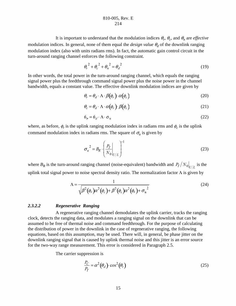
For the example composite code of Paragraph 2.2.2.1, the s of Equation (38) is plotted in Figure 5 and the Pacq of Equation (41) is plotted in Figure 6. For Figure 5, the range

clock is a 1 MHz sinewave. The abscissa for both figures is the product �� ◊ ��

, expressed

in decibels: �� ◊ ��

� �

Ê Ë Á ˆ

¯ ˜ . Comparing Figures 5 and 6, it becomes clear that this

example composite code was designed to give a range measurement error (due to thermal noise) of about 0.1 to 0.2 meter when

�� ◊ ��

is just large enough to assure a high probability of

acquisition.

For the example composite code of Paragraph 2.2.2.2, the s of Equation (38) is plotted in Figure 7 and the Pacq of Equation (41) is plotted in Figure 8. For Figure 7, the range

clock is a 1 MHz sinewave. The abscissa for both figures is the product �� ◊ ��

, expressed

in decibels: �� ◊ ��

� �

Ê Ë Á ˆ

¯ ˜ . Comparing Figures 7 and 8, it becomes clear that this

example composite code was designed to give a range measurement error (due to thermal noise) of about 5.0 to 6.0 meters when

�� ◊ ��

is just large enough to assure a high probability of

acquisition.

In comparing the two example composite codes, some important observations can be made. The composite code of Paragraph 2.2.2.1 requires a much larger value for

�� ◊ ��

in order to assure acquisition, but the range measurement error (due to thermal

noise) is quite small, in the neighborhood of 0.1 to 0.2 meter. That composite code is suitable for regenerative ranging. The composite code of Paragraph 2.2.2.2, on the other hand, may be acquired with a much smaller value for

�� ◊ ��

; so this second composite code is a better

choice for turn-around ranging. Of course, with the smaller �� ◊ ��

, the range

measurement error will necessarily be larger.

2.5.2 Noncoherent Operation

A noncoherent ranging technique has been described in Reference 7. For the sake of economy, this technique employs a transceiver, rather than a transponder, at the spacecraft. With such a technique, the downlink carrier is not coherent with the uplink carrier, and the downlink range clock is not coherent with the downlink carrier. This means that there will ordinarily be a frequency mismatch between the received downlink range clock and its local model. This mismatch is to be minimized by Doppler compensation of the uplink carrier, but it will not be possible, in general, to eliminate completely the frequency mismatch. With this noncoherent technique, range measurement performance will not be as good as that which can be achieved with coherent operation using a transponder. Nonetheless, noncoherent range measurement performance is expected to be adequate for some mission scenarios.

810-005, Rev. E 214

26

Figure 5. Range Measurement Error for the Composite Code of Paragraph 2.2.2.1

810-005, Rev. E 214

27

Figure 6. Probability of Acquisition for the Composite Code of Paragraph 2.2.2.1

810-005, Rev. E 214

28

Figure 7. Range Measurement Error for the Composite Code of Paragraph 2.2.2.2

810-005, Rev. E 214

29

Figure 8. Probability of Acquisition for the Composite Code of Paragraph 2.2.2.2

810-005, Rev. E 214

30

The frequency mismatch inherent in noncoherent ranging has two effects on performance. One is a loss Ac of correlation amplitude, which increases the thermal noise contribution to measurement error. The other is a direct contribution to range measurement error. This direct contribution is much the more important of these two effects.

The loss of correlation amplitude is represented by the term Ac, where 0 < Ac < 1. The standard deviation s of range measurement error due to thermal noise is given by Equation (38), and the probability of acquisition (considering the effect of thermal noise) is given by Equations (41) and (42). The amplitude loss factor Ac is, for noncoherent operation, given by (see Reference 7)

��

= "��$ �D��( ) (45)

where DfRC is the frequency mismatch between the received range clock and its local model and

T is the measurement integration time. The function sinc(.) is defined by Equation (33). (With coherent operation, DfRC = 0 and Ac = 1.)

The direct contribution of frequency mismatch to range measurement error is given by (see Reference 7)

%�� %%�%�� #��D �� = ��◊ D ��

�� ◊ � (46)

It is worth noting that this measurement error is directly proportional to both the fractional frequency mismatch ��D �� and the measurement integration time T. The fractional frequency error will, in general, comprise two terms: a fractional frequency error due to uncertainty in the spacecraft oscillator frequency and a fractional frequency error due to imperfect uplink Doppler predicts.

Noncoherent ranging measurements should be done with regenerative ranging using pseudo-noise signals. The reason for this follows. The direct error contribution due to frequency mismatch is directly proportional to the measurement integration time, as can be seen in Equation (46). So, for noncoherent operation, it is important to make T as small as possible. This is achieved with regenerative ranging, and regenerative ranging is only available with a pseudo-noise ranging signal.

With noncoherent operation, the range error due to frequency mismatch increases with T and the range error due to thermal noise decreases with T. Therefore, it is important to seek an optimal value for T, in order to get the best possible performance. Reference 7 offers guidance in this matter.

2.6 Range Corrections

The DTT range measurements include delays of equipment within the DSS as well as those of the spacecraft. These delays must be removed in order to determine the actual range referenced to some designated location at the antenna. Figure 9 illustrates the end-to-end

810-005, Rev. E 214

31

Figure 9. DSN Range Measurement

range measurement and identifies the delays that must be removed before an accurate topocentric range can be established. The DSN is responsible for providing three measurements to the project. They are the DSS delay, the Z-correction, and the antenna correction.

2.6.1 DSS Delay

The DSS delay is station and configuration dependent. It should be measured for every ranging pass. This measurement is called precal for pre-track calibration and postcal for post-track calibration. The former is done at the beginning of a ranging pass; the latter is only needed when there is a change in equipment configuration during the track or precal was not performed due to a lack of time.

810-005, Rev. E 214

32

The delay is measured by a test configuration, which approximates the actual ranging configuration. The signal is transmitted to the sky; however, before reaching the feedhorn, a sample is diverted to a test translator through a range calibration coupler. The test translator shifts the signal to the downlink frequency, which is fed into a coupler ahead of the LNA. The signal flows through the LNA to the DTT for calibration.

Figure 10 shows the signal path for a typical calibration of DSS delay when the uplink and downlink are in the same frequency band. The heavy lines identify the calibration path. When the uplink and downlink are in different bands, the downlink signal from the test translator is coupled into the receive path ahead of the LNA and as close to the feed as practical.

2.6.2 Z-Correction

The delay in the microwave components between the range calibration coupler or couplers and the airpath (the distance from the horn aperture plane to the subreflector, to the antenna aperture plane, and finally to the antenna reference location) must be included in the calibration. Also, the translator delay must be removed. A Z-correction takes care of these items. This Z-correction is given by the difference of two quantities: the translator delay and the microwave plus air path delay. The microwave and air path delays are determined from a combination of laboratory and physical measurements.

The test translator delay is measured by connecting a zero delay device (ZDD) to the couplers that are normally connected to the test translator. Since the ZDD and its interconnecting cable delays are measured in the laboratory, the signal delay contributed by the test translator can be calculated to a known precision. This measurement is made approximately once each year or when there are hardware changes in the signal path.

2.6.3 Antenna Correction

An antenna correction is required when the primary and secondary antenna axes do not intersect with the result being that the antenna reference location is not at a fixed location with respect to the Earth. The only DSN antenna where an antenna correction is necessary is the 34-m High-speed Beam Waveguide antenna, DSS 27. The antenna correction for DSS 27 can be calculated from the following expression

��Dr� =��$�"q , m (47)

where q is the antenna elevation angle.

2.7 Ground Instrumentation Error Contribution

The ground system, the media, and the spacecraft contribute errors to range measurements. The error contributions of the media and spacecraft are outside the scope of this document and have not been included. The error due to thermal noise is discussed in Paragraph 2.5. This paragraph estimates the error contribution from ground instrumentation, excepting thermal noise.

810-005, Rev. E 214

33

Figure 10. Typical DSS Delay Calibration

The round-trip one-sigma delay error of the DSN ranging system over a ranging pass has been estimated for the X-band system as 6.3 nanoseconds (about 0.95 meter one-way). The S-band one-sigma delay error has been estimated as 12.5 nanoseconds (about 1.9 meters one-way).

Table 7 provides a breakdown of long-term error contributions due to calibration and errors inherent within the equipment of the various subsystems that constitute the total DSS ground ranging system. The line item Reserve accounts for the measurement error uncertainties.

Change 1: March 31, 2004

810-005, Rev. E 214

34

Table 7. Ground Instrumentation Range Error for NSP Era Ranging System

X-band S-band

Subsystem Round-trip

Delay (ns)

One-way

Distance (m)

Round-trip Delay

(ns)

One-way

Distance (m)

FTS 1.00 0.15 1.00 0.15

Receiver 2.00 0.30 2.00 0.30

Exciter and Transmitter 1.33 0.20 5.33 0.80

Microwave and Antenna 2.33 0.35 2.33 0.35

Uplink Ranging Board 2.00 0.30 2.00 0.30

Downlink Ranging Board 2.00 0.30 2.00 0.30

Cables 1.33 0.20 1.33 0.20

Calibration 2.66 0.40 2.66 0.40

Reserve 3.33 0.50 10.0 1.50

Root Sum Square 6.33 0.95 12.47 1.87

Change 1: March 31, 2004

810-005, Rev. E 214

35

References

1. S. Bryant, “Using Digital Signal Processor Technology to Simplify Deep Space Ranging,” 2001 IEEE Aerospace Conference, March 10-17, 2001, Big Sky, MT.

2. J. B. Berner and S. H. Bryant, “New Tracking Implementation in the Deep Space Network,” 2nd ESA Workshop on Tracking, Telemetry and Command Systems for Space Applications, October 29-31, 2001, Noordwijk, The Netherlands.

3. J. B. Berner, J. M. Layland, P. W. Kinman, and J. R. Smith, “Regenerative Pseudo-Noise Ranging for Deep-Space Applications,” TMO Progress Report 42-137, Jet Propulsion Laboratory, Pasadena, CA, May 15, 1999.

4. J. B. Berner, P. W. Kinman, and J. M. Layland, “Regenerative Pseudo-Noise Ranging for Deep Space Applications,” 2nd ESA Workshop on Tracking, Telemetry and Command Systems for Space Applications, October 29-31, 2001, Noordwijk, The Netherlands.

5. J. B. Berner and S. H. Bryant, “Operations Comparison of Deep Space Ranging Types: Sequential Tone vs. Pseudo-Noise,” 2002 IEEE Aerospace Conference, March 9-16, 2002, Big Sky, MT.

6. P. W. Kinman and J. B. Berner, “Two-Way Ranging During Early Mission Phase,” 2003 IEEE Aerospace Conference, March 8-15, 2003, Big Sky, MT.

7. M. K. Reynolds, M. J. Reinhart, R. S. Bokulic, “A Two-Way Noncoherent Ranging Technique for Deep Space Missions,” 2002 IEEE Aerospace Conference, March 9-16, 2002, Big Sky, MT.

Documents

214 Pseudo-Noise and Regenerative Ranging