212 Unstructured Grid Generation - CCG · Unstructured Grid Generation in 2-D and 3-D S. Fatemeh Razavi, Jeff Boisvert, Juliana Leung Numerical modeling is used to predict flow behavior

Paper 212, CCG Annual Report 13, 2011 (© 2011)

212-1

Unstructured Grid Generation in 2-D and 3-D

S. Fatemeh Razavi, Jeff Boisvert, Juliana Leung

Numerical modeling is used to predict flow behavior and simulate transport phenomena. One of the origins of

complexity in a geological media is the existence of a large number of fractures. An efficient discritization of the

fracture media is required. This Discritization or mesh generation requires significant preprocessing effort. The

objective of this paper is meshing these complex fracture structures in 2D and 3D essential for future simulation

purposes. A program was developed to generate unstructured triangular mesh for a randomly generated discrete

fracture network in 2-D and TetGen program was used to generate mesh for a 3-D discrete fracture network. On 3-

D grids, geostatistical modeling is done to populate the grids with permeability values.

1. Introduction

There are two approaches to model flow and mass transport in fractured porous media, dual continuum model

proposed by warren & Root in 1963 and discrete fracture model (DFM). DFM is a reasonable method to model

laboratory scale fractured porous media (Ito, 2003).

Considering reservoir heterogeneities mainly included discrete fracture networks is the main focus of this

research. The goal is simulation on the unstructured grids, which has been populated with permeability and

porosity values by Geostatistical methods, to obtain effective permeability tensor that can be used for flow

simulations at a coarse scale. This is important because current computational capabilities do not permit flow

simulation on a field-scale DFM model containing hundreds or thousands of fractures. Flow is considered along the

fractures and that’s why creating grids aligned fractures is of importance.

Unstructured grids are suitable choice to grid design that have the required flexibility to handle domains

with complicated geometries and boundaries. One of the remarkable advantages of unstructured grids is

possibility of controlling the grid resolution through refinement. Taking into account, the geometrical simplicity

and the accessible procedures for the numerical simulation of physical problems (Liseikin, 2010), unstructured

grids are generally composed of triangles in two dimensions and tetrahedrons in three dimensions. Basically, three

methods exist to construct unstructured grids including Octree methods, Delaunay procedures and Advancing

Front techniques (Liseikin, 2010).

Delaunay tessellation is a more common geometric decomposition tool to generate triangular and

tetrahederal grids that has found wide use in engineering applications. Two and three-dimensional Delaunay

tessellations are used for the analysis of porous media, and the modeling of flow in porous media (Thompson,

2002). Liseikin’s book is a good reference to get information about the two other methods for unstructured mesh

generation.

The present work is chiefly included obtaining a reasonable Delaunay mesh for a flexible discrete fracture

network in 2D and 3D. There are different open access programs to mesh complex geological media. Some of them

are listed and explained in brief in the following.

DistMesh is a simple MATLAB code for generation of unstructured triangular and tetrahedral meshes uses

Delaunay triangulation and tetrahedralization. It was developed by the Department of Mathematics at MIT. A

detailed description of the program is provided in Per-Olof Persson and Gilbert Strang, 2004 (DistMesh weblog).

This code could be modified based on needs.

G23FM is another grid generator for 2D and 3D fractured media which generates unstructured grids

automatically. It was introduced as a flexible tool including different options like adding points, controlling

triangles sizes, refinement and scaling (Mustapha, 2010) and developed by a computer science specialist at McGill

University.

FracMesh is a 2-D and 3-D structured mesh generator developed by Earth Sciences Division at Berkley.

The most complicated part of fracture network gridding is creating the connectivity list. FracMesh produces the

connectivity lists necessary for the input file of the multiphase flow numerical simulator TOUGH2 (Ito, 2003).

TetGen and Triangle are two well-tested mesh generators for 3D tetrahedral and 2D triangular meshing.

TetGen was developed by Numerical Mathematics and Scientific Computing group at WIAS which could generate

conforming Delaunay tetrahedra and apply volume control. Triangle was developed by Computer Science Division

at Berkley (Triangle weblog: http://www.cs.cmu.edu/~quake/triangle.html).


212-2

MeshPy combines TetGen with Triangle into one package, which is very practical and was developed at

the Institute of Mathematical Sciences at New York University (http://mathema.tician.de/software/meshpy).

Because of no availability of G23FM software when requested, considering this point that FractMesh is for

structured grid generation while we are interested in unstructured mesh generation and mainly TetGen good

quality manual, we selected TetGen for mesh generation in 3-D.

This paper is organized as follows; in the second part, Delaunay criterion will be explained. In the third

part, unstructured mesh generation for 2D DFM will be described in detail. In fourth part, mesh generation for a

3D DFM is discussed and in the fifth part, 3-D grids are populated with permeability.

2. Delaunay Triangulation and Tetrahedralization

Based on Delaunay triangulation, neighboring points are connected to form triangular or tetrahederal cells in such

a way that the circumcircle through the three vertices of a triangular cell in two-dimension and the circumsphere

through the four vertices of a tetrahedral cell in three-dimension do not contain any other point. This condition is

called Delaunay criterion (see Figure 1). In fact by applying Delaunay criterion in 2D, the minimum angle of all the

angles of the triangles in the triangulation will be maximized and the maximum circumradius will be minimized

thus they tend to avoid skinny triangles which will result in optimal triangulation in 2D and more refinement will be

unnecessary (Liseikin, 2010). Note that, the Delaunay Triangulation is not unique. Optimal properties of Delaunay

triangulation are not true in 3D, since a measurement for optimality in 3D is not agreed on. Slivers are special type

of badly-shaped tetrahedrons which are flat and nearly degenerate and they will cause instability and

inconsistency. In 3D, slivers could survive even after Delaunay refinement. To measure quality of tetrahedrons in

3D, two criterion is considered: 1) aspect ratio of an element which should be as small as possible and defined as

ratio of the maximum side length to the minimum altitude, 2) radius edge ratio, which is the ratio of the radius of

the circumsphere of the tetrahedron to the length of the shortest edge. This value should be small for a well-

shaped tetrahederon.

3. Unstructured Mesh Generation in 2-D

In the first part, two cases are considered, including fracture with thickness and fracture without thickness.

Subsequently, the focus of the second part is on the generation of a flexible fractured model in 2D by finding

suitable points distribution on fractures to populate them as straight lines and moreover finding suitable

background point distribution to show the matrix. Then, the resulted points distribution follows by automatic

Delaunay triangulation done by Matlab DelaunayTri uses CGAL, the Computational Geometry Algorithms Library.

To display the triangles defined by DelaunayTri, Matlab triplot function is used

3.1. Part I: Considering a Single Fracture

Fractures are lines including two endpoints in 2D and planes including four endpoints in 3D. Investigations started

in two-dimension. Points were distributed uniformly in two steps, in background and on fractures for two different

cases: 1) Fractures with thickness and 2) Fractures without thickness.

The following considerations play significant roles in accurate point distribution:

1) Removing background points close to the distributed points on fractures is essential.

2) In case of fracture with thickness, one should consider three parallel lines to represent the fracture and its

thickness.

3) Boundary treatment is inevitable to calculate the accurate starting points for point distributions started

from boundaries.

3.1.1. Boundary Treatment

Goal is obtaining equilateral triangles around fracture. For starting a correct distribution of points from boundaries,

a geometric problem have to be solved. Consider left side of three parallel lines representative of one fracture with

thickness (see Figure 2). Firstly, points on the middle line is to be distributed (points a, d …) and based on the

resulted distribution, the exact place of starting point on upper and lower lines (around middle line) is calculated.

X1 and X2 are target unknowns in Figure 2.

in ∆ abc: ab = X1 , ab = ac * cos(<cao + <dak)

< dak = arctan(fracture slope)


212-3

in ∆ aco : ac = sqrt(ht ^ 2 + ao ^ 2) = sqrt(ht ^ 2 + (spacing / 2) ^ 2)

<cao = arctan(ht / ao)

in ∆ anm: nm = X3, nm = am * cos(<dak - <oam) = ac * cos(<dak - <cao)

X3 – X2 = em * cos(<dak) = ao * cos(<dak)

In Figure 2, ht is equal to half of the fracture thickness and “cm” is the perpendicular bisector of “ad”. By

calculating the angles <dak, <cao and the length ac, X1 and X2 is obtained which are starting points on upper line

and lower line respectively.

After applying uniform point distribution, boundary treatment and removing close background points

around fracture. Mesh is generated and visualized by using Matlab “DelaunayTri” and “triplot” commands

respectively (see Figure 3). It is important to note that figure 3 can be easily representative of fracture without

thickness if background mesh and fracture thickness mesh have relatively close size. While for fractures with

thickness, there is a transition (buffer) zone around fracture with medium grid size showing the transition of fine

grid size around fractures to background coarse mesh size. To represent the transition zone, around three main

lines (in the middle) two more lines were populated by points considering suitable point distances q times bigger

than the half of the main fracture thickness (ht in Figure 2). “q” is named scaling factor (see Figure 4).

Generally, considering fracture thickness at point distribution stage is not necessary because fracture

grids can be added based on the technique proposed by Karimi Fard (SPE 79699) to consider flow along the

fractures so we are ignoring the thickness in the next section.

3.2.Part II: 2D Discrete Fractured Network Modeling

Main goal in this section is to generate a flexible discrete fracture network without considering the fractures

thickness and more importantly populating them with suitable point distribution to have acceptable mesh. Most of

the required programs for this part had been written in part I and just some generalizations were necessary.

The same as previous part, distribution of background points and fractures population should be done

separately (each of them in a separate function). Before fractures population, considering several fractures in

fractured model, the intersections of n fractures are calculated by using the endpoints of fractures (see Figure 5 as

a sample) slope and interception for each fracture. Subsequently, points are distributed on each fracture between

endpoints and intersections and based on a feasible distance entered by user as “d” (see Figure 6). “d” which is the

distance between distributed points have to be corrected on each segment of a fracture, for instance, fracture in

Figure 5, includes 5 segments). This correction is done by defining a correction factor. In Figure 7, “L” is the length

of each segment on one fracture. The endpoints of the solid line in Figure 7 are the endpoints of on fracture. The

middle white point is an intersection and red point is the first distributed point on the RHS segment. Consider that

this fracture has two segments.

Correction Factor (CF) = L / (d * round (L / d))

Note that “d” is the same for all fractures and the projection of d multiplied by CF on X axis should be

used for point distribution. Figure 8 is shown both point distribution and mesh results before and after applying

this correction. When one intersection coincided with an endpoint (Figure 9), fracture population stops. This

problem is solved by using a separate function applied to the matrix which lists all points on the related fracture. In

fact, in the point lists matrix including the endpoints, intersections and distributed points, repeated points are

removed.

By applying all the mentioned modifications, the following fractured model was created as a sample

(Figure 10). Fractures are generated stochastically and randomly. Point distribution on a fracture, which is

orthogonal to x axis, needs different attention and it is done in a separate function.

In the next step, the close background points should be removed. This is done by a flexible criterion which

has dependency on “d”. Background points after removing the close ones is shown in Figure 11.

Figure 13 is showing mesh result for combination of fractures and background points (shown in Figure 12)

generated by Delaunay tessellation. Mesh is generated by Matlab DelaunayTri and visualized by Matlab “triplot”.

As a quick note, the input data for running the program are the number of fractures, endpoints of

fractures (planes could be generated randomly as well), feasible distance between distributed points on fractures


212-4

(d), Length of the square area and the number of background points in x and y directions (nx and ny), which are

regularly the same. Finding a general relation between nx (ny) and d and additionally a relation between the

criterion for removing the BG points and d is recommended as future work to improve the results.

4. Unstructured Mesh Generation in 3-D

4.1. Developing Codes

In 3D, the same procedure could be applied to generate random 3D fracture planes, populating them with suitable

uniform point distribution, distribute points on 3D background and removing the BG points close to the fracture

planes based on a suitable criterion. A single randomly generated fracture plane populated uniformly with points,

a sample generated random DFM with 30 fractures and distributed points on 3D background can be seen in

Figures 14, 15 and 16. For now, TetGen will be used to generate mesh for a 3D DFM.

4.2. Unstructured 3D Mesh Generation by TetGen

TetGen produces tetrahedral meshes suitable for numerical simulation which are using finite volume or finite

element methods. Terahedralization is done based on Delaunay criterion. In TetGen, constrained Delaunay

Triangulation could be applied which decomposes a 3D domain into a tetrahedral mesh, such that the boundary is

presented in the faces of the mesh.

The quality of tetrahedrons is measured by two criteria, aspect ratio of the element and radius edge ratio.

It is important to note that while some of the degenerated tetrahedra, slivers, can be removed by TetGen using

local flip technique; still slivers could survive even after Delaunay refinement. In the following, you will see some

quick notes for using TetGen: As an input, TetGen uses a general input called piecewise linear complex (PLC). A PLC

is including a set of vertices, a set of segments and facets. See Figure 18. The pink area shows a facet which is non-

convex, has a hole, segments and vertices in it, (Si, 2006). Then by using the suitable command executable in

Cygwin, mesh will be generated. A simple TetGen command is as follows:

Program Switch/Switches Input

./tetgen.exe –p *.poly

Both input file and output files could be visualized. To visualize the input and output of TetGen, TetView

program is normally used. Input file is a “*.poly” file including the information of the facets, segments and points

of the PLC. A typical output will include a list of mesh nodes (*.node), a list of tetrahedral (*.ele) and a list of

boundary faces/convex hull faces (*.face). It is important to note that convex hull is represented by a list of

triangles as well. To generate mesh for our case which is a DFM, fracture planes should be created randomly in the

first step and then intersections of the fracture planes have to be found.

4.2.1. Generating Fracture Planes

To define a DFM in TetGen, each fracture plane is defined as a facet. The vertices used to define a facet of a PLC

have to be precisely coplanar, but it is hard to achieve (Si, 2006). So, TetGen accepts the endpoints of a plane

which are approximately coplanar and this approximation is defined by a tolerance. The suitable endpoints of a

fracture plane can be achieved based on the following criterion for coplanar test:

V / L3 < Tolerance

Where V is the Volume of the tetrahedron abcd created by four endpoints a, b, c and d and L is the

average edge length of tetrahedron abcd. Default tolerance value in TetGen is 1e-8. One can set a tolerance for

coplanar test by “-T” switch. It is appealing that by applying “-M” switch, TetGen does not merge coplanar fracture

planes (facets).

4.2.2. Detecting the Intersections Between Fracture Planes

There is a very useful possibility in TetGen which helps to detect intersections of the PLC facets. For a DFM

including numerous fracture planes, we need to know the intersection of each two fracture planes to add that

intersection segment as a polygon when defining each fracture plane for TetGen. Finding the intersections is done


212-5

by creating a “*.node” file including the endpoints of the generated DFM and running TetGen program with “-d”

switch on the “*.node” file as an input.

Program Switch Input

./tetgen.exe –d *.node

4.2.3. Creating TetGen Input File

After generating the fracture planes and finding the intersections, “*.poly” file should be created. It is including

four parts and the information of all the nodes, segments and facets. The intersection nodes will be added to the

first part of the file which is node list and the intersecting segments will be added in the second part which is a list

of facets. Facet list should be created very carefully. See two invalid facets in the Figure 17. The facets are invalid

because one segment (which is intersecting line) including two intersection points is missing in both planes. Each

of the planes should be defined as two polygons not a single polygon. The first polygon is including the four

endpoints and the 2nd

one is the segment including two intersecting points.

A typical input file for a sample DFM with 7 fractures can be seen in Figure 19. Hole list and region list

which are parts 3 and 4 of the input file, are empty for this example. TetGen visualized input file created by

Tetview is shown in Figure 20. The right hand side image is a typical input DFM of FracMesh. The curved-shaped

fracture plane (the green one in the RHS image) was created by combination of small pieces of rectangular fracture

planes with different normal vectors and corner points (Si, 2006).

4.2.4. Getting Output and Visualization

In the following, is a sample command executed in Cygwin to generate tetrahedral mesh.

Program Switch/Switches Input

./tetgen.exe –pq1.414a0.5f *.poly

It is really important to note that to have a list of all facies “-f” switch should be used. By “-p” command

mesh is generated and “-q” imposes the quality constraint and adds more points rather than using “-p” only.

Radius edge ratio should be written after “-q” switch and default value for this ratio is considered 2 by TetGen.

Maximum volume constraint is applied by entering a number after “-a” switch. In the above command, by applying

a0.5, we constrain the maximum volume of the tetrahedrons to be less than 0.5 cubic meters. It is possible to

reconstruct and refine previously generated mesh by “-r” and adding a list of additional points by applying “-i”

switch. To visualize the input and output files, the following sample commands could be used:

Program Input

Input visualization: ./tetview-win *.poly

Output visualization: ./tetview-win *.1

*.1 is including all output information (nodes, edges, faces) for “*.poly” input file. TetView-win is a version

of TetView compatible with windows operation system. TetGen typical outputs including a list of nodes, faces and

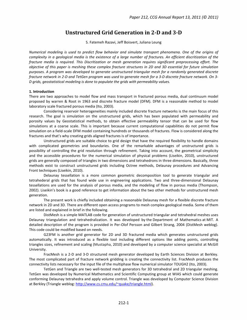
tetrahedrons are shown in Figure 21. A sample visualized output for a DFM including 7 fractures can be seen in

Figure 22. Fracture planes are recognizable by marking them using boundary marker option (Si, 2006). It is possible

to visualize the output of TetGen in Medit or Gid as well. To see TetGen results under Medit “-g” and to see the

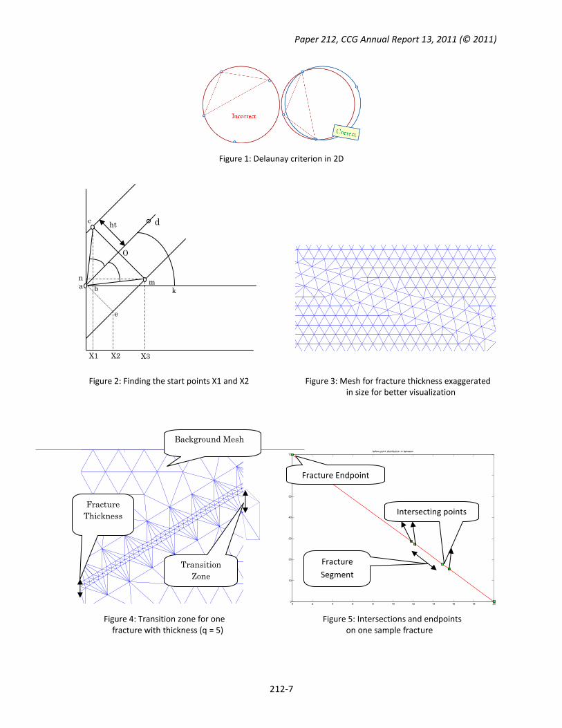
results under Gid, “-G” switches should be used. Quality report of generated mesh is obtainable by “-V” switch or

using the following command. A sample mesh quality statistics can be seen in Figure 23.

Program Switches

. / tetgen.exe –rNEFV


212-6

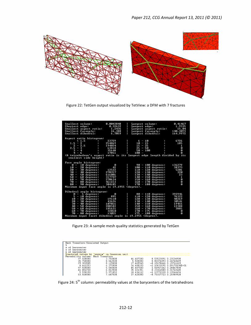
5. Permeability Distribution of Elements

Geostatistical modeling of petrophysical properties is done by using a GSLib program named “psgsim” (Manchuk,

2010). PSGSIM is to perform sequential Gaussian simulation of continuous variables and sequential indicator

simulation of categorical properties on irregular sets of points. These sets of points are the location of the

unknowns which are petrophysical properties. These locations in the triangular/tetrahedral control volumes in

2D/3D could be:

A) At the center of the unique circumcircle/circumsphere of each triangle/tetrahedron or,

B) At the centroid, named also geometric center, center of mass, center of gravity or barycenter of each

triangle/tetrahedron.

For our case, grids’ barycenter have been calculated and then populated with permeability values (See

Figure 24).

6. Conclusions

Unstructured meshing was done for randomly generated 2D DFM. Codes are flexible and details have been

presented in the first part of the paper. By comparison with similar works done previously using G23FM

(Mustapha, 2010) and DistMesh (Bajaj, 2009), our results are remarkably practical while still some modifications

could be done to improve the results. Unstructured mesh generation for a 3D DFM is done by applying TetGen

program. A sample DFM model with seven fractures meshed by TetGen and resulted tetrahedral grids were

populated with permeability values using geostatistical modeling.

References

Bajaj, R., 2009, “An Unstructured Finite Volume Simulator For Multiphase Flow Through Fractured-Porous Media”,

MSc Thesis, MIT University,

Ito K. and Seol Y., 2003, “A 3-Dimensional Discrete Fracture Network Generator to Examine Fracture-Matrix

Interaction Using TOUGH2”, Berkeley, California,

Liseikin, V.D., 2010, “Grid Generation Methods”, Book, Springer, Second Edition,

Manchuk, J., 2010, “Geostatistical Modeling of Unstructured Grids for Flow Simulation”, PhD thesis, University of

Alberta,

Mustapha, H., 2010, “G23FM: a tool for meshing complex geological media”, Springer,

Persson P. and Strang G., 2004, “A Simple Mesh Generator in Matlab”, http://persson.berkeley.edu/distmesh/,

Si, H., 2006, “A Quality Tetrahedral Mesh Generator and Three-Dimensional Delaunay Triangulator”,

http://tetgen.berlios.de/,

Thompson, K.E., 2002, “Fast and robust Delaunay tessellation in periodic domains”, Wiley Publication.


212-7

Figure 1: Delaunay criterion in 2D

Figure 2: Finding the start points X1 and X2 Figure 3: Mesh for fracture thickness exaggerated

in size for better visualization

Figure 4: Transition zone for one Figure 5: Intersections and endpoints

fracture with thickness (q = 5) on one sample fracture

k

X1 X3

ht

O

m n a

c

e

b

X2

d

0 2 4 6 8 10 12 14 16 18 200

10

20

30

40

50

60

70before point distribution in between

Fracture

Segment

Intersecting points

Fracture Endpoint

Transition

Zone

Fracture

Thickness

Background Mesh


212-8

Figure 6: Population of fracture in figure 4 Figure 7

a) Before applying CF b) After applying CF

a) Before applying CF b) After applying CF

Figure 8: Removing degenerated triangles by applying correction factor

0 2 4 6 8 10 12 14 16 18 200

10

20

30

40

50

60

70after point distribution in between

d L


212-9

Figure 9 Figure 10: a sample DFM in two-dimension

including horizontal and vertical fractures

Figure 11: BG points after removing points Figure 12: Both fractures and BG points

close to the fracture points

Figure 13: Delaunay mesh results

(Area Length = 100, nx = ny = 50, d = 1.5, criteria < 0.5d)

Intersection endpoint

0 10 20 30 40 50 60 70 80 90 1000

10

20

30

40

50

60

70

80

90

100

0 10 20 30 40 50 60 70 80 90 1000

10

20

30

40

50

60

70

80

90

100BG Points after Removing Close Points

0 10 20 30 40 50 60 70 80 90 1000

10

20

30

40

50

60

70

80

90

100All Points (Faults & BG) after Removing Close BG Points

0 10 20 30 40 50 60 70 80 90 1000

10

20

30

40

50

60

70

80

90

100


212-10

Figure 14: A sample randomly generated fracture plane Figure 15: 3D background point distribution

where points distributed on it uniformly

Figure 16: A randomly generated DFM with 30 fractures

(The green color is because of point distribution on the planes)

Figure 17: Two invalid facets (fracture planes) Figure 18: A sample PLC: TetGen input (Si, 2006)

as TetGen input


212-11

Figure 19: TetGen typical input file (*.poly)

Figure 20: An example of input 3D DFM in a) TetGen and b) FracMesh (Ito, 2003)

Figure 21: TetGen typical output including nodes, faces and tetraheda lists


212-12

Figure 22: TetGen output visualized by TetView: a DFM with 7 fractures

Figure 23: A sample mesh quality statistics generated by TetGen

Figure 24: 5th

column: permeability values at the barycenters of the tetrahedrons

Documents

212 Unstructured Grid Generation - CCG · Unstructured Grid Generation in 2-D and 3-D S. Fatemeh Razavi, Jeff Boisvert, Juliana Leung Numerical modeling is used to predict flow behavior