Embed Size (px)
Citation preview

21 Aug 2007
KKKQ 3013KKKQ 3013PENGIRAAN BERANGKAPENGIRAAN BERANGKA
Week 7 ndash Interpolation amp Curve Fitting21 August 2007
800 am ndash 900 am
21 Aug 2007 Week 7 Page 2
Topics
1048713 Introduction1048713 Newton Interpolation Finite Divided Difference1048713 Lagrange Interpolation1048713 Spline Interpolation1048713 Polynomial Regression1048713 Multivariable Interpolation
21 Aug 2007 Week 7 Page 3
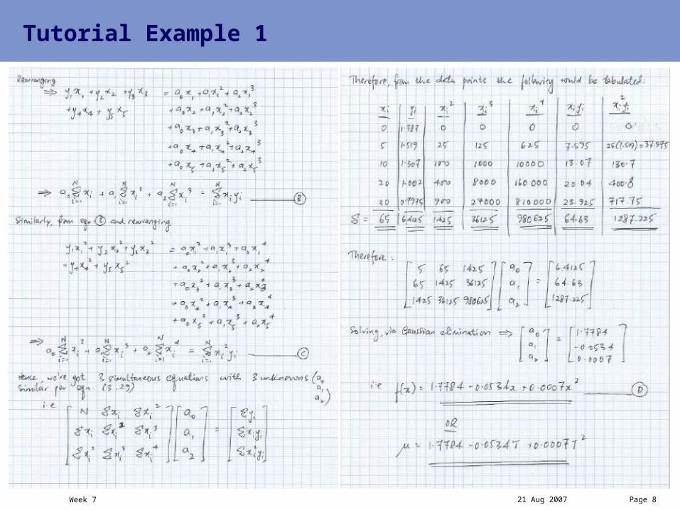
Tutorial Example 1 (adapted courtesy of ref [1])
Dynamic viscosity of water (10-3 Nsm2) is related to temperature T(oC) in the following manner
[1] Chapra SC amp Canale RP Numerical Methods for Engineers McGraw-Hill 5th ed (2006)
a) Estimate at T = 75oC using cubic spline interpolation
b) Use polynomial regression to determine a best fit parabola of the above data In addition determine the corresponding standard deviation
Based on this parabola what is at T = 75oC
21 Aug 2007 Week 7 Page 4
Tutorial Example 1
21 Aug 2007 Week 7 Page 5
Tutorial Example 1
21 Aug 2007 Week 7 Page 6
Tutorial Example 1
21 Aug 2007 Week 7 Page 7
Tutorial Example 1
21 Aug 2007 Week 7 Page 8
Tutorial Example 1
21 Aug 2007 Week 7 Page 9
Tutorial Example 1
21 Aug 2007 Week 7 Page 10
Tutorial Example 1 (using MATLAB)
gtgt x=[0 5 10 20 30]
x =
0 5 10 20 30
gtgt y=[1787 1519 1307 1002 07975]
y =
17870 15190 13070 10020 07975
gtgt a=interp1(xy75spline)
a =
14069
gtgt p=polyfit(xy2)
p =
00007 -00534 17784
gtgt b=polyval(p75)
b =
14172
Prediction using cubic spline interpolation
Coefficient for best fit quadratic equation ie a2 a1 and a0 in descending powers of x

21 Aug 2007 Week 7 Page 2
Topics
1048713 Introduction1048713 Newton Interpolation Finite Divided Difference1048713 Lagrange Interpolation1048713 Spline Interpolation1048713 Polynomial Regression1048713 Multivariable Interpolation
21 Aug 2007 Week 7 Page 3
Tutorial Example 1 (adapted courtesy of ref [1])
Dynamic viscosity of water (10-3 Nsm2) is related to temperature T(oC) in the following manner
[1] Chapra SC amp Canale RP Numerical Methods for Engineers McGraw-Hill 5th ed (2006)
a) Estimate at T = 75oC using cubic spline interpolation
b) Use polynomial regression to determine a best fit parabola of the above data In addition determine the corresponding standard deviation
Based on this parabola what is at T = 75oC
21 Aug 2007 Week 7 Page 4
Tutorial Example 1
21 Aug 2007 Week 7 Page 5
Tutorial Example 1
21 Aug 2007 Week 7 Page 6
Tutorial Example 1
21 Aug 2007 Week 7 Page 7
Tutorial Example 1
21 Aug 2007 Week 7 Page 8
Tutorial Example 1
21 Aug 2007 Week 7 Page 9
Tutorial Example 1
21 Aug 2007 Week 7 Page 10
Tutorial Example 1 (using MATLAB)
gtgt x=[0 5 10 20 30]
x =
0 5 10 20 30
gtgt y=[1787 1519 1307 1002 07975]
y =
17870 15190 13070 10020 07975
gtgt a=interp1(xy75spline)
a =
14069
gtgt p=polyfit(xy2)
p =
00007 -00534 17784
gtgt b=polyval(p75)
b =
14172
Prediction using cubic spline interpolation
Coefficient for best fit quadratic equation ie a2 a1 and a0 in descending powers of x