Embed Size (px)
Citation preview
202: Dynamic MacroeconomicsDynamic Ineffi ciency & Technical Progress in Solow Model
Mausumi Das
Delhi School of Economics
January 21-22, 2015
Das (Delhi School of Economics) Dynamic Macro January 21-22, 2015 1 / 34
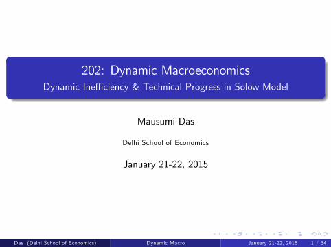
Solow Model: Growth Implications
In the long run (at steady state),
per capita income of the economy does not grow;aggregate income grows at a constant rate - given by the exogenousrate of growth of population (n);government policies to increase the savings ratio has no long rungrowth affect.
In the short run (during transition),
per capita income of the economy grows due to capital accumulation -but the growth rate keeps declining;aggregate income grows due to both capital accumulation andpopulation growth;the further away the economy is from its steady state, the higher is itsgrowth rate;government policies to increase the savings ratio temporarily increasesthe growth rate, since it raises the steady state value of k as well asthe transitional growth rate.
Das (Delhi School of Economics) Dynamic Macro January 21-22, 2015 2 / 34
Critique of Solow Model: does it explain ‘growth’?
The fundamental critisism of the Solow ‘growth’model is that it failsto explain long run growth:
The per capita income does not grow at all in the long run;The aggregate income grows at an exogenously given rate n, which themodel does not attempt to explain.
The short run growth of per capita income is explained by capitalaccumulation.But capital accumulation happens in the Solow model because, byassumption, households perpetually save a fixed proportion oftheir income - irrespective of the rate of return.It is not clear why households will keep accumulating capital - in theface of a falling rate of return!! (Recall that as k increases r ≡ f ′(k)keeps declining.)This seems irrational. Surely there is some cost to savings! If nothingelse, the households might be better off consuming the extra outputrather than saving it - especially if the rate of return of capital is toolow!
Das (Delhi School of Economics) Dynamic Macro January 21-22, 2015 3 / 34
Critique of Solow Model (Contd.):
In fact the assumed constancy of the savings ratio in the Solow modelgenerates another problem - that of dynamic ineffi ciency.What is dynamic effi cinecy/ineffi ciency?
It is a conecpt similar to Pareto effi ciency/ineffi ciency - but used in anintertemporal sense.
An economic situation is ‘dynamically ineffi cient’if we can improvethe welfare of the agents in all future dates, without reducing theircurrent welfare. The economy is ‘dynamically effi cient’otherwise.(Remember agents are identical here; so improving welfare of oneimples improving welfare of all.)
Das (Delhi School of Economics) Dynamic Macro January 21-22, 2015 4 / 34
Solow Model: Golden Rule & Dynamic Ineffi ciency
To understand concept of dynamic effi ciency in the Solow model, letus now got back to long run steady state of Solow.Recall that for given values of δ and n, the savings rate in theeconomy uniquely pins down the corresponding steady statecapital-labour ratio:
k∗(s) :f (k∗)k∗
=n+ δ
s.
We have already seen that a higher value of s is associated with ahigher k∗, and therefore, a higher level of steady state per capitaincome (f (k∗)).How about the corresponding level of consumption?Notice that in this model, per capita consumption is defined as:
CtNt
≡ Yt − StNt
⇒ ct = f (kt )− sf (kt )Das (Delhi School of Economics) Dynamic Macro January 21-22, 2015 5 / 34
Golden Rule & Dynamic Ineffi ciency in Solow Model(Contd.)
Accordingly, for given values of δ and n, steady state level of percapita consumption is related to the savings ratio of the economy inthe following way:
c∗(s) = f (k∗(s))− sf (k∗(s))= f (k∗(s))− (n+ δ) k∗(s). [Using the definition of k∗]
We have already noted that if the government tries to manipulate thesavings ratio (by imposing an appropriate tax onconsumption/savings), then such a policy has no long run growtheffect.Can such a policy still generate a higher level of steady state percapita consumption at least?If yes, then such a policy would still be desirable, even if it does notimpact on growth.
Das (Delhi School of Economics) Dynamic Macro January 21-22, 2015 6 / 34
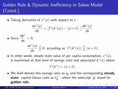
Golden Rule & Dynamic Ineffi ciency in Solow Model(Contd.)
Taking derivative of c∗(s) with respect to s :
dc∗(s)ds
=[f ′(k∗(s))− (n+ δ)
] dk∗(s)ds
.
Sincedk∗
ds> 0,
dc∗(s)ds
T 0 according as f ′(k∗(s)) T (n+ δ).
In other words, steady state value of per capita consumption, c∗(s),is maximised at that level of savings ratio and associated k∗(s) where
f ′(k∗) = (n+ δ).
We shall denote this savings ratio as sg and the corresponding steadystate capital-labour ratio as k∗g - where the subscript ‘g’stand forgolden rule.
Das (Delhi School of Economics) Dynamic Macro January 21-22, 2015 7 / 34
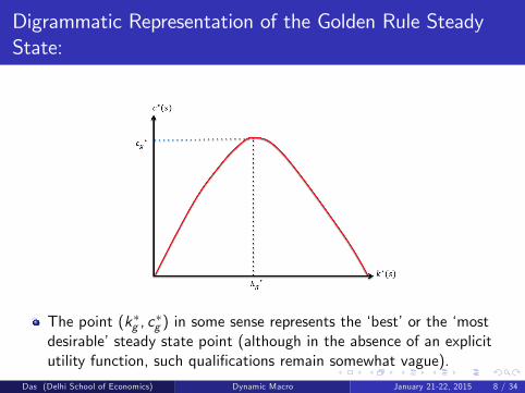
Digrammatic Representation of the Golden Rule SteadyState:
The point (k∗g , c∗g ) in some sense represents the ‘best’or the ‘most
desirable’steady state point (although in the absence of an explicitutility function, such qualifications remain somewhat vague).
Das (Delhi School of Economics) Dynamic Macro January 21-22, 2015 8 / 34
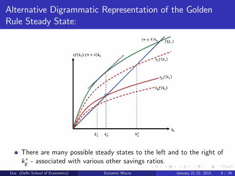
Alternative Digrammatic Representation of the GoldenRule Steady State:
There are many possible steady states to the left and to the right ofk∗g - associated with various other savings ratios.
Das (Delhi School of Economics) Dynamic Macro January 21-22, 2015 9 / 34
Golden Rule & the Concept of ‘Dynamic Ineffi ciency’
Importantly, all the steady states to the right of k∗g are called‘dynamically ineffi cient’steady states.From any such point one can ‘costlessly’move to the left - to alower steady state point - and in the process enjoy a higher level ofcurrent consumption as well as higher levels of future consumption atall subsequent dates. (How?)Notice however that the steady states to the left of k∗g are not‘dynamically ineffi cient’. (Why not?)
Das (Delhi School of Economics) Dynamic Macro January 21-22, 2015 10 / 34
Cause of ‘Dynamic Ineffi ciency’in Solow Model
Notice that dynamic ineffi ciency occurs because people oversave.
This possibility arises in the Solow model because the savings ratio isexogenously given - it is not chosen through households’optimizationprocess.
If the steady state of an economy indeed happens to be dynamicallyineffi cient, then it justifies an active, interventionist role of thegovernment in the Solow model - even though government cannotaffect the long run rate of growth of the economy.
Das (Delhi School of Economics) Dynamic Macro January 21-22, 2015 11 / 34
Limitations of the Solow Growth Model:
Even though the Solow model is supposed to be a growth model - itcannot really explain long run growth:
The per capita income does not grow at all in the long run;The aggregate income grows at an exogenously given rate n, which themodel does not attempt to explain.
The steady state in the Solow model might be dynamically ineffi cient.It is not clear why households will not correct this ineffi cinency bychoosing their savings ratio optimally. But this latter possibility issimply not allowed in the Solow model.
Das (Delhi School of Economics) Dynamic Macro January 21-22, 2015 12 / 34
Extensions of Solow Growth Model:
The basic Solow growth model has subsequently been extended tocounter some of these critisisms.
The primary challenge is to retain the basic result of the Solow model(namely, existence of a unique and globally stable steady state) whilerelaxing various restrictive assumptions.
We shall look at two such extensions:1 Solow Model with Technological Progress: This extension allows theper capita income to grow in the long run; developed by Solow himself(Solow (1957)).
2 Neoclassical Growth Model with Optimizing Households: Thisextension allows the households to choose their consumption/savingsbehaviour optimally over infinite horizon; developed independently byCass (1965) & Koopmans (1965).
Das (Delhi School of Economics) Dynamic Macro January 21-22, 2015 13 / 34
Solow Model with Exogenous Technological Progress:
Let us now introduce a productivity-specific parameter into ourSolovian firm-specific production function:
Yit = F (Kit ,Nit ,At );FA > 0,
where F satisfies all the standard Neoclassical properties specifiedearlier.The term At captures the state of the technology at time t. Since allfirms have access to identical technology, this technology-specificparameter is the same for all firms (hence no i-subscript here).The assumption of identical firms and CRS implies that the aggregateproduction function will also take similar form:
Yt = F (Kt ,Nt ,At );FA > 0.
Technological progress implies that the productivity-specific term, At ,increases in value over time. Thus with the same amount of labourand capital, the economy can now produce greater amount of output.
Das (Delhi School of Economics) Dynamic Macro January 21-22, 2015 14 / 34

Different Types of Technological Progress:
Technological progress can be of three types:1 Labour Augmenting or Harrod-Neutral: Technical improvementenhances the productivity of labour alone:
Yt = F (Kt ,AtNt ).
2 Capital Augmenting or Solow-Neutral: Technical improvementenhances the productivity of capital alone:
Yt = F (AtKt ,Nt ).
3 Capital & Labour Augmenting or Hicks-Neutral: Technicalimprovement enhances the productivity of both capital and labour inequal proportion and thus augments total factor productivity:
Yt = F (AtKt ,AtNt ) = AtF (Kt ,Nt ).
Notice that with Cobb-Douglas Production Function, all the threenotions of technical progress are equivalent. (Prove this.)
Das (Delhi School of Economics) Dynamic Macro January 21-22, 2015 15 / 34
Technological Progress and Balanced Growth:
Modern Growth Theory often focuses on Balanced Growth Path: ascenario when every variable in the economy grows at some constantrate (not necessarily equal for all variables).
Recall that steady state is also a special case of balanced growth(when the growth rate is constant at 0).
It can be shown that unless the production function is Cobb-Douglas,only Harrod-neutral technological progress is consistent with abalanced growth path. (Proof follows a few slides later.)Henceforth, we shall therefore restrict our analysis only toHarrod-neutral technological progress.
Das (Delhi School of Economics) Dynamic Macro January 21-22, 2015 16 / 34
Solow Model with Harrod-Neutral Technological Progress:
Suppose all assumptions of the original Solow model remainunchanged, except that we now have a firm-specific productiontechnology, given by:
Yit = F (Kit ,AtNit ).
The corresponding aggregate production technology is given by
Yt = F (Kt ,AtNt ) ≡ F (Kt , Nt ),where we denote the productivity-augmented labour term: AtNt ≡ Nt(effective labour).Labour productivity increases automatically over time (like ‘mannafrom heaven’) at an exogenous rate m:
1At
dAdt= m.
Each firm now equates the marginal product of ‘effective labour’withthe wage rate per unit of ‘effective labour’(w) and the marginalproduct of capital with the rental rate of capital (r).
Das (Delhi School of Economics) Dynamic Macro January 21-22, 2015 17 / 34
Solow Model with Harrod-Neutral Technological Progress(Contd.):
CRS and identical firms implies that the firm-specific marginalproduct and the (social) marginal product for the aggregate economyare the same.Thus we get the aggregate demand functions for ‘effective labour’and capital as:
FN (Kit , Nit ) = FN (Kt , Nt ) = wt ;
FK (Kit , Nit ) = FK (Kt , Nt ) = rt .
At the beginning of any time period t, the economy starts with agiven stock of population (Nt), a given stock of capital (Kt) and agiven level of labour productivity (At).The wage rate per unit of effective labour and rental rate adjust sothat that there is full employment of the given endowment of effectivelabour and capital stock at every point of time t.
Das (Delhi School of Economics) Dynamic Macro January 21-22, 2015 18 / 34
Capital- Effective Labour Ratio & Output per unit ofEffective Labour:
Using the CRS property, we can write:
yt ≡YtNt=F (Kt ,AtNt )
AtNt= F
(KtAtNt
, 1)≡ f (kt ),
where yt represents output per unit of effective labour, and ktrepresents the capital-effective labour ratio in the economy at time t.
Using the relationship that F (Kt , Nt ) = Nt f (kt ), we can easily showthat:
FN (Nt ,Kt ) = f (kt )− kt f ′(kt ) = wt ;FK (Nt ,Kt ) = f ′(kt ) = rt .
[Derive these two expressions yourselves].
Das (Delhi School of Economics) Dynamic Macro January 21-22, 2015 19 / 34
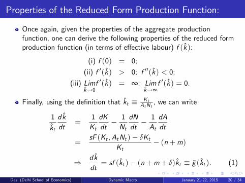
Properties of the Reduced Form Production Function:
Once again, given the properties of the aggregate productionfunction, one can derive the following properties of the reduced formproduction function (in terms of effective labour) f (k):
(i) f (0) = 0;
(ii) f ′(k) > 0; f ′′(k) < 0;
(iii) Limk→0
f ′(k) = ∞; Limk→∞
f ′(k) = 0.
Finally, using the definition that kt ≡ KtAtNt
, we can write
1
kt
dkdt
=1Kt
dKdt− 1Nt
dNdt− 1At
dAdt
=sF (Kt ,AtNt )− δKt
Kt− (n+m)
⇒ dkdt= sf (kt )− (n+m+ δ)kt ≡ g(kt ). (1)
Das (Delhi School of Economics) Dynamic Macro January 21-22, 2015 20 / 34
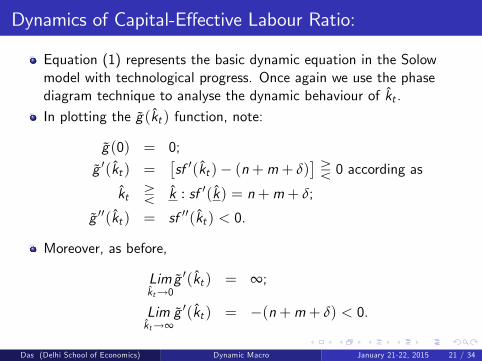
Dynamics of Capital-Effective Labour Ratio:
Equation (1) represents the basic dynamic equation in the Solowmodel with technological progress. Once again we use the phasediagram technique to analyse the dynamic behaviour of kt .
In plotting the g(kt ) function, note:
g(0) = 0;
g ′(kt ) =[sf ′(kt )− (n+m+ δ)
]R 0 according as
kt R k : sf ′(k) = n+m+ δ;
g ′′(kt ) = sf ′′(kt ) < 0.
Moreover, as before,
Limkt→0
g ′(kt ) = ∞;
Limkt→∞
g ′(kt ) = −(n+m+ δ) < 0.
Das (Delhi School of Economics) Dynamic Macro January 21-22, 2015 21 / 34
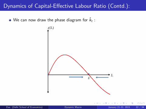
Dynamics of Capital-Effective Labour Ratio (Contd.):
We can now draw the phase diagram for kt :
Das (Delhi School of Economics) Dynamic Macro January 21-22, 2015 22 / 34
Dynamics of Capital-Effective Labour Ratio (Contd.):
From the phase diagram we can identify two possible steady states:
(i) k = 0 (Trivial Steady State);
(ii) k = k∗ > 0 (Non-trivial Steady State).
As before, ignoring the non-trivial steady state, we get a uniquenon-trivial steady state, k∗, which is globally asymptotically stable:starting from any initial capital-effective labour ratio k0 > 0, theeconomy would always move to k∗ in the long run.
Implication:
In the long run, output per unit of effective labour: yt ≡ f (kt ) will beconstant at f (k∗).
Das (Delhi School of Economics) Dynamic Macro January 21-22, 2015 23 / 34
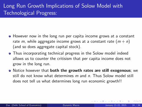
Long Run Growth Implications of Solow Model withTechnological Progress:
However now in the long run per capita income grows at a constantrate m, while aggregate income grows at a constant rate (m+ n)(and so does aggregate capital stock).
Thus incorporating technical progress in the Solow model indeedallows us to counter the critisism that per capita income does notgrow in the long run.
Notice however that both the growth rates are still exogenous; westill do not know what determines m and n. Thus Solow model stilldoes not tell us what determines long run economic growth!!
Das (Delhi School of Economics) Dynamic Macro January 21-22, 2015 24 / 34
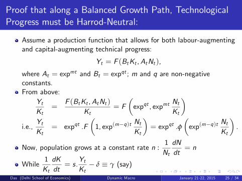
Proof that along a Balanced Growth Path, TechnologicalProgress must be Harrod-Neutral:
Assume a production function that allows for both labour-augmentingand capital-augmenting technical progress:
Yt = F (BtKt ,AtNt ),
where At = expmt and Bt = expqt ; m and q are non-negativeconstants.From above:
YtKt
=F (BtKt ,AtNt )
Kt= F
(expqt , expmt
NtKt
)i.e.,
YtKt
= expqt .F(1, exp(m−q)t
NtKt
)= expqt .φ
(exp(m−q)t
NtKt
).
Now, population grows at a constant rate n :1Nt
dNdt= n
While1Kt
dKdt= s.
YtKt− δ ≡ γ (say)
Das (Delhi School of Economics) Dynamic Macro January 21-22, 2015 25 / 34
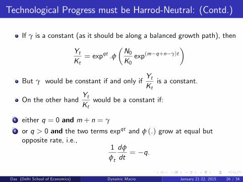
Technological Progress must be Harrod-Neutral: (Contd.)
If γ is a constant (as it should be along a balanced growth path), then
YtKt= expqt .φ
(N0K0exp(m−q+n−γ)t
)
But γ would be constant if and only ifYtKt
is a constant.
On the other handYtKt
would be a constant if:
1 either q = 0 and m+ n = γ
2 or q > 0 and the two terms expqt and φ (.) grow at equal butopposite rate, i.e.,
1φt
dφ
dt= −q.
Das (Delhi School of Economics) Dynamic Macro January 21-22, 2015 26 / 34
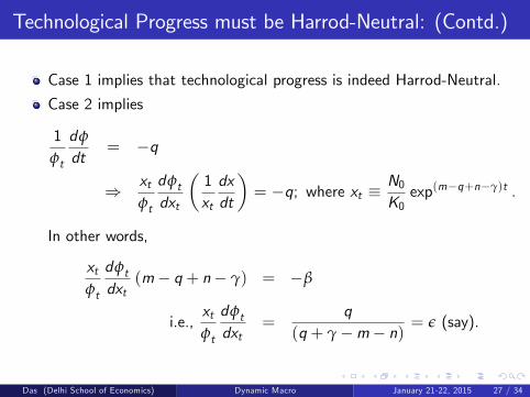
Technological Progress must be Harrod-Neutral: (Contd.)
Case 1 implies that technological progress is indeed Harrod-Neutral.
Case 2 implies
1φt
dφ
dt= −q
⇒ xtφt
dφtdxt
(1xt
dxdt
)= −q; where xt ≡
N0K0exp(m−q+n−γ)t .
In other words,
xtφt
dφtdxt
(m− q + n− γ) = −β
i.e.,xtφt
dφtdxt
=q
(q + γ−m− n) = ε (say).
Das (Delhi School of Economics) Dynamic Macro January 21-22, 2015 27 / 34
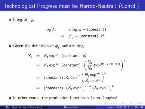
Technological Progress must be Harrod-Neutral: (Contd.)
Integrating,
log φt = ε log xt + (constant)
⇒ φt = (constant) .xεt
Given the definition of φt , substituting,
Yt = Kt expqt . (constant) .xεt
= Kt expqt . (constant) .(N0K0exp(m−q+n−γ)t
)ε
= (constant) .Kt expqt(Nt expmt
Kt expqt
)ε
= (constant) .(Kt expqt
)1−ε (Nt expmt)ε
In other words, the production function is Cobb-Douglas!
Das (Delhi School of Economics) Dynamic Macro January 21-22, 2015 28 / 34
Long Run Growth of Per Capita Income withoutTechnological Progress?
Exogenous technological progress is not a very satisfactory way togenerate long run growth of per capita income in the Solow model.
Without a proper theory to explain this phenomenon, it remains amere technical exercise.
Moreover the fact that only Harrod-neutral technical progress isconsistent with the Solow-type long run steady state also seems tolimit the applicability of the model.
Can we have long run growth of per capita income in the Solowmodel - even without exogenous technical progress?
The answer is: yes, but only if you allow some of the Neoclassicalproperties of the production function to be relaxed.
Das (Delhi School of Economics) Dynamic Macro January 21-22, 2015 29 / 34
Growth of Per Capita Income without Technical Progress:(Contd.)
Recall that the long run constancy of the per capita income in theSolow model arises due to the strong uniqueness and stability propertyof the steady state - which in turn depends on two key assumptions:the property of diminishing returns and the Inada Conditions.We can have long run growth of per capita income in the Solowmodel even without technological progress only if we are willing torelax at least one of these two key assumptions.
Das (Delhi School of Economics) Dynamic Macro January 21-22, 2015 30 / 34
Growth of Per Capita Income without Technical Progress:(Contd.)
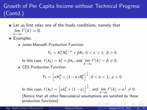
Let us first relax one of the Inada conditions, namely thatlimk→∞
f ′(k) = 0.
Examples:Jones-Manuelli Production Function:
Yt = K αt N
1−αt + βKt ; 0 < α < 1; β > 0.
In this case, f (kt ) = kαt + βkt ; and lim
k→∞f ′(k) = β 6= 0.
CES Production Function:
Yt =[αK ρ
t + (1− α)Nρt
] 1ρ; 0 < α < 1; ρ > 0.
In this case, f (kt ) =[αkρt + (1− α)
] 1ρ; and lim
k→∞f ′(k) = α
1ρ 6= 0.
(Notice that all other Neocalssical assumptions are satisfied by theseproduction functions)
Das (Delhi School of Economics) Dynamic Macro January 21-22, 2015 31 / 34

Growth of Per Capita Income without Technical Progress(Contd.):
While there is no natural justification for the Inada conditions, (andmost well-known production functions, except the Cobb-Douglas,typically violate one of these), relaxing only the Inada conditions maynot generate a balanced growth path. (Recall our obsession withbalanced growth!!)Another way to generate long run growth of per capita income in theSolow model without technological progress is to do away with theassumption of diminishing returns altogether (i.e., f ′′(k) ≮ 0).An example of non-dinimishing returns but CRS production functionis the linear technology case:
Yt = AKt + BNt ; A,B > 0.
A special case of linear technology - AK production function:
Yt = AKt ; A > 0.
Das (Delhi School of Economics) Dynamic Macro January 21-22, 2015 32 / 34
Growth of Per Capita Income without Technical Progress(Contd.):
Replacing the Neoclassical production function in the Solow model bythe AK production technology indeed generates a balanced growthpath.
Rate of growth of per capita output in this case (in long as well asshort run) is:
sA− (n+ δ)
Notice that now the government can directly affect the growth rate ofthe economy by influencing the savings ratio!
There are several interesting economic justifications for this kind ofAK production technology.
We shall examine some of these justifications later in the course.
Das (Delhi School of Economics) Dynamic Macro January 21-22, 2015 33 / 34
Solow Model with Exogenous Technical Progress & AKTechnology : Reference
Robert Barro & Xavier Sala-i-Martin: Economic Growth, 2004 (2ndEdition), The MIT Press, Chapter 1.
Das (Delhi School of Economics) Dynamic Macro January 21-22, 2015 34 / 34