Embed Size (px)
Citation preview

© 2019 - Shivang
BRUSHLESS DOUBLY-FED RELUCTANCE MACHINE DRIVE FORTURBO-ELECTRIC DISTRIBUTED PROPULSION SYSTEMS
BY
- SHIVANG
THESIS
Submitted in partial fulfillment of the requirementsfor the degree of Master of Science in Electrical and Computer Engineering
in the Graduate College of theUniversity of Illinois at Urbana-Champaign, 2019
Urbana, Illinois
Adviser:
Assistant Professor Arijit Banerjee
ABSTRACT
Turbo-electric distributed propulsion systems are considered to be a crit-
ical enabler for low-carbon emission in the aircraft industry. A brushless
doubly-fed reluctance machine (BDFRM) is an attractive option to drive the
distributed propeller fans for these megawatt-scale turbo-electric propulsion
systems due to use of a partially-rated power converter, reduced maintenance,
and absence of permanent magnets. This thesis investigates the torque pro-
duction in BDFRM, discusses machine modeling and drive control architec-
ture, and reports on an initial sizing of a 1.5 MW motor. However, the
BDFRM has inherently poor torque density because of machine saturation,
even at low current-density, that offsets all the benefits. This thesis proposes
an approach to maximize the torque density by finding appropriate electri-
cal excitations on the two stator windings for a given machine dimension
while remaining within flux- and current-density limits. A single-objective
optimization problem is formulated. The obtained results prove that while
designs with equal electrical loadings on both stators, and an initial current
phase offset of π/2 between the two stators, may seem a good design ap-
proach, they are far from optimal. Our optimized solution establishes that
the phase offset of 2π/3 provides maximum torque capability for an identical
dimension. This procedure is validated using FEA simulations. Operating
with this design also leads to higher machine efficiency and better power fac-
tor on the secondary stator, thus reducing the converter rating. Finally, the
thesis concludes with a summary of findings and suggestions for future work
in this field.
ii

To my family, for their constant support.
And to the many friends, new and old, I have made along the way.
iii

ACKNOWLEDGMENTS
First and foremost, I would like to acknowledge my family who always have
been there, continuously supporting my education. Being so far away from
them has not always been easy but they have continued to have their faith
in me, motivate me for further success and always believe in me.
I would like to express my sincere gratitude to my supervisor Prof. Arijit
Banerjee for his patience, motivation and immense knowledge. The support,
guidance and academic freedom he provided allowed me to develop skills that
will surely help me become a successful engineer, leader, and mentor. His
careful and precious guidance was extremely valuable for my study. I was
also lucky to be a Teaching Assistant with him in ECE 464. Watching him
teach in the class so passionately helped me enhance my teaching skills.
I want to express my gratitude to Raymond Beach at NASA Glenn Re-
search Center for giving me the opportunity to work on such a cool project
in my first year of MS. The Grainger Center for Electric Machinery and Elec-
tromechanics has always been there for us to provide the financial support
we needed.
To the awesome power group, thank you for being great co-workers and
friends. The power group here at Illinois is something very unique and will
always hold a special place in my heart. You guys made sure that I stick
around for a couple of more years and do my PhD here at Illinois.
I perceive the opportunity to do my MS at UIUC as a big milestone in
my career development. I will strive to use skills and knowledge gained here
in the best possible way, and I will continue to work on improving them, in
order to attain my desired career objectives.
iv
TABLE OF CONTENTS
CHAPTER 1 INTRODUCTION . . . . . . . . . . . . . . . . . . . . 1
CHAPTER 2 STEADY-STATE ANALYSIS . . . . . . . . . . . . . . 62.1 Air-gap flux density distribution with different rotor structures 72.2 Machine inductances . . . . . . . . . . . . . . . . . . . . . . . 10
CHAPTER 3 DYNAMIC MODEL . . . . . . . . . . . . . . . . . . . 123.1 Model in ABC framework . . . . . . . . . . . . . . . . . . . . 133.2 α - β transformation . . . . . . . . . . . . . . . . . . . . . . . 153.3 d-q model . . . . . . . . . . . . . . . . . . . . . . . . . . . . . 183.4 Torque computation . . . . . . . . . . . . . . . . . . . . . . . 193.5 Speed computation . . . . . . . . . . . . . . . . . . . . . . . . 21
CHAPTER 4 DRIVE CONTROL ARCHITECTURE . . . . . . . . . 224.1 Stator flux estimation . . . . . . . . . . . . . . . . . . . . . . . 224.2 Current controllers design . . . . . . . . . . . . . . . . . . . . 234.3 Speed controller . . . . . . . . . . . . . . . . . . . . . . . . . . 264.4 Reactive power controller . . . . . . . . . . . . . . . . . . . . . 26
CHAPTER 5 ELECTROMAGNETIC DESIGN METHODOLOGY . 285.1 D2l sizing derivation . . . . . . . . . . . . . . . . . . . . . . . 285.2 Dl sizing derivation . . . . . . . . . . . . . . . . . . . . . . . . 325.3 Example design of a 1.5 MW BDFRM . . . . . . . . . . . . . 33
CHAPTER 6 TORQUE DENSITY IMPROVEMENT . . . . . . . . 366.1 Optimization problem formulation . . . . . . . . . . . . . . . . 386.2 Impact of optimization on torque density . . . . . . . . . . . . 396.3 Impact of optimization on power converter size . . . . . . . . . 426.4 Impact of optimization on grid and converter power factor . . 46
CHAPTER 7 FINITE ELEMENT ANALYSIS AND RESULTS . . . 50
CHAPTER 8 CONCLUSIONS . . . . . . . . . . . . . . . . . . . . . 558.1 Summary and design insights . . . . . . . . . . . . . . . . . . 558.2 Future work . . . . . . . . . . . . . . . . . . . . . . . . . . . . 56
v

APPENDIX A ELECTROMAGNETIC TORQUE PRODUCEDBY BDFRM . . . . . . . . . . . . . . . . . . . . . . . . . . . . . . . 57
APPENDIX B DETERMINATION OF KP AND KI BASED ONFIRST-ORDER SYSTEM . . . . . . . . . . . . . . . . . . . . . . . 60
REFERENCES . . . . . . . . . . . . . . . . . . . . . . . . . . . . . . . 61
vi
CHAPTER 1
INTRODUCTION
The U.S. aviation industry produces 11% of total transportation-related
emissions domestically, and about 3% of the global CO2 emissions annu-
ally are produced by planes. Substantial improvements in air transportation
technologies continue to increase the efficiency of air transportation by mov-
ing passengers and cargo over the same distance with less fuel consumed and,
hence, fewer carbon emissions. The International Civil Aviation Organiza-
tion anticipates a 3x increase in the global international aviation emissions
by 2050 [1]. This exponential increase in the air travel has prompted a signif-
icant effort to mitigate the impact of commercial aviation on climate change.
At the request of the National Aeronautics and Space Administration
(NASA), the National Academies of Sciences, Engineering, and Medicine
convened a committee to develop a national research agenda for reducing
CO2 emissions from commercial aviation, focusing on single-aisle and twin-
aisle large commercial aircraft. They proposed four high-priority approaches
that could reduce CO2 emissions and could be implemented during the next
10 to 30 years [2]:
� Advances in aircraft–propulsion integration,
� Improvements in gas turbine engines,
� Development of turbo-electric distributed propulsion (TeDP) systems,
and
� Advances in sustainable alternative jet fuels.
This thesis focuses on the development of turbo-electric propulsion systems.
These propulsion systems employ gas turbines to drive electric generators,
which deliver power to several motors driving a set of distributed propeller
fans. The propeller thrust is regulated by controlling the individual motor
1
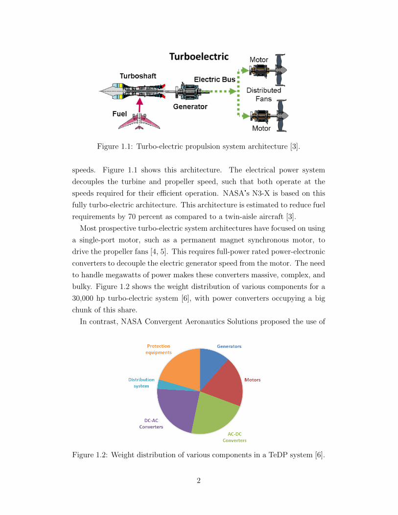
Figure 1.1: Turbo-electric propulsion system architecture [3].
speeds. Figure 1.1 shows this architecture. The electrical power system
decouples the turbine and propeller speed, such that both operate at the
speeds required for their efficient operation. NASA's N3-X is based on this
fully turbo-electric architecture. This architecture is estimated to reduce fuel
requirements by 70 percent as compared to a twin-aisle aircraft [3].
Most prospective turbo-electric system architectures have focused on using
a single-port motor, such as a permanent magnet synchronous motor, to
drive the propeller fans [4, 5]. This requires full-power rated power-electronic
converters to decouple the electric generator speed from the motor. The need
to handle megawatts of power makes these converters massive, complex, and
bulky. Figure 1.2 shows the weight distribution of various components for a
30,000 hp turbo-electric system [6], with power converters occupying a big
chunk of this share.
In contrast, NASA Convergent Aeronautics Solutions proposed the use of
Figure 1.2: Weight distribution of various components in a TeDP system [6].
2
a doubly-fed machine (DFM), both as a generator and a motor, by adopting
a high-voltage, wide-range variable frequency ac power distribution architec-
ture [7]. This architecture reduces the power-electronic converter requirement
by 85% as compared to the one with single-port machines — an advantage
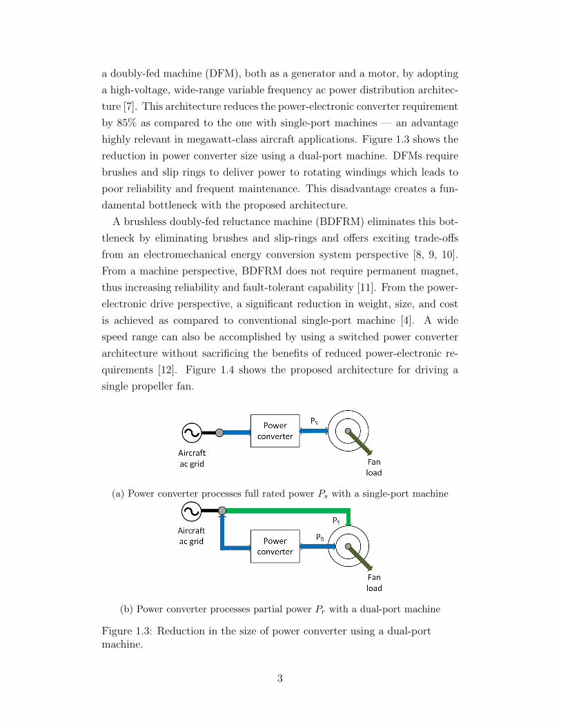
highly relevant in megawatt-class aircraft applications. Figure 1.3 shows the
reduction in power converter size using a dual-port machine. DFMs require
brushes and slip rings to deliver power to rotating windings which leads to
poor reliability and frequent maintenance. This disadvantage creates a fun-
damental bottleneck with the proposed architecture.
A brushless doubly-fed reluctance machine (BDFRM) eliminates this bot-
tleneck by eliminating brushes and slip-rings and offers exciting trade-offs
from an electromechanical energy conversion system perspective [8, 9, 10].
From a machine perspective, BDFRM does not require permanent magnet,
thus increasing reliability and fault-tolerant capability [11]. From the power-
electronic drive perspective, a significant reduction in weight, size, and cost
is achieved as compared to conventional single-port machine [4]. A wide
speed range can also be accomplished by using a switched power converter
architecture without sacrificing the benefits of reduced power-electronic re-
quirements [12]. Figure 1.4 shows the proposed architecture for driving a
single propeller fan.
(a) Power converter processes full rated power Ps with a single-port machine
(b) Power converter processes partial power Pr with a dual-port machine
Figure 1.3: Reduction in the size of power converter using a dual-portmachine.
3
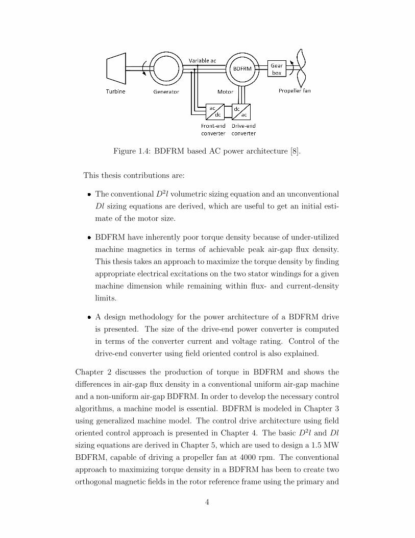
Figure 1.4: BDFRM based AC power architecture [8].
This thesis contributions are:
� The conventional D2l volumetric sizing equation and an unconventional
Dl sizing equations are derived, which are useful to get an initial esti-
mate of the motor size.
� BDFRM have inherently poor torque density because of under-utilized
machine magnetics in terms of achievable peak air-gap flux density.
This thesis takes an approach to maximize the torque density by finding
appropriate electrical excitations on the two stator windings for a given
machine dimension while remaining within flux- and current-density
limits.
� A design methodology for the power architecture of a BDFRM drive
is presented. The size of the drive-end power converter is computed
in terms of the converter current and voltage rating. Control of the
drive-end converter using field oriented control is also explained.
Chapter 2 discusses the production of torque in BDFRM and shows the
differences in air-gap flux density in a conventional uniform air-gap machine
and a non-uniform air-gap BDFRM. In order to develop the necessary control
algorithms, a machine model is essential. BDFRM is modeled in Chapter 3
using generalized machine model. The control drive architecture using field
oriented control approach is presented in Chapter 4. The basic D2l and Dl
sizing equations are derived in Chapter 5, which are used to design a 1.5 MW
BDFRM, capable of driving a propeller fan at 4000 rpm. The conventional
approach to maximizing torque density in a BDFRM has been to create two
orthogonal magnetic fields in the rotor reference frame using the primary and
4

secondary stator windings, similar to a uniform air gap sinusoidal machine
[8, 13]. In this design approach, the allowable current density is implicitly
restricted by the flux density limit rather than independent thermal design
considerations. Fundamentally, this unconventional limit on the allowable
current density is due to the non-sinusoidal air-gap flux density distribution
in a BDFRM, which comprises several spatial harmonics.
Chapter 6 opens up the design space by allowing the angle between the
two magnetic fields to be varied to increase the current density towards the
thermal-consideration-driven constraint. Intuitively, this angle is similar to
the definition of torque angle in a synchronous machine. An optimization
problem is formulated to maximize the output torque while choosing the
electrical loadings on both stators as design variables. Operating flux density,
current density, grid voltage, and machine dimensions are used to set the
design constraints. The machine torque capability is enhanced by 75% for an
identical machine dimension [14] while simultaneously improving the power
factor of the secondary stator, and hence reducing the power converter size.
The overall efficiency also increases with the proposed design. The simulation
results as carried out using ANSYS Maxwell are presented in Chapter 7 and
decisively prove the benefits proposed in theory. The conclusions and future
work are provided in Chapter 8.
5
CHAPTER 2
STEADY-STATE ANALYSIS
A brushless doubly-fed machine (BDFM) works on the principle of air-gap
flux modulation. The machine has two stator windings, commonly known
as primary or grid winding and secondary or control winding, with different
pole numbers. An induction-based or a reluctance-based rotor modulates
the air-gap field to couple the two stator windings [15]. These two classes
of machines have been denoted as brushless doubly-fed induction machine
(BDFIM) and brushless doubly-fed reluctance machine (BDFRM). The lat-
ter, with a radially laminated reluctance rotor with flux guides, will be con-
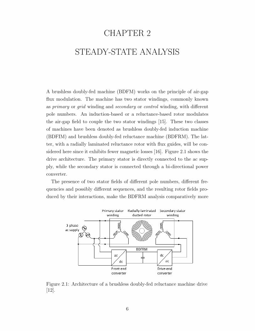
sidered here since it exhibits fewer magnetic losses [16]. Figure 2.1 shows the
drive architecture. The primary stator is directly connected to the ac sup-
ply, while the secondary stator is connected through a bi-directional power
converter.
The presence of two stator fields of different pole numbers, different fre-
quencies and possibly different sequences, and the resulting rotor fields pro-
duced by their interactions, make the BDFRM analysis comparatively more
Figure 2.1: Architecture of a brushless doubly-fed reluctance machine drive[12].
6
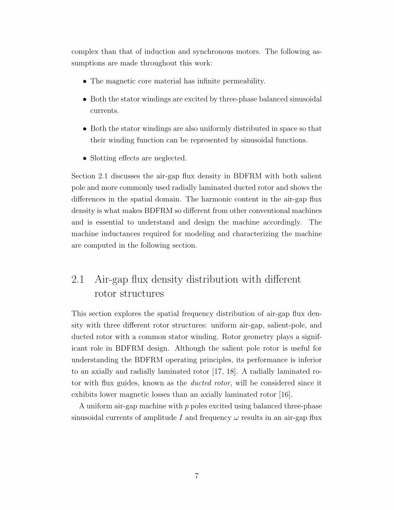
complex than that of induction and synchronous motors. The following as-
sumptions are made throughout this work:
� The magnetic core material has infinite permeability.
� Both the stator windings are excited by three-phase balanced sinusoidal
currents.
� Both the stator windings are also uniformly distributed in space so that
their winding function can be represented by sinusoidal functions.
� Slotting effects are neglected.
Section 2.1 discusses the air-gap flux density in BDFRM with both salient
pole and more commonly used radially laminated ducted rotor and shows the
differences in the spatial domain. The harmonic content in the air-gap flux
density is what makes BDFRM so different from other conventional machines
and is essential to understand and design the machine accordingly. The
machine inductances required for modeling and characterizing the machine
are computed in the following section.
2.1 Air-gap flux density distribution with different
rotor structures
This section explores the spatial frequency distribution of air-gap flux den-
sity with three different rotor structures: uniform air-gap, salient-pole, and
ducted rotor with a common stator winding. Rotor geometry plays a signif-
icant role in BDFRM design. Although the salient pole rotor is useful for
understanding the BDFRM operating principles, its performance is inferior
to an axially and radially laminated rotor [17, 18]. A radially laminated ro-
tor with flux guides, known as the ducted rotor, will be considered since it
exhibits lower magnetic losses than an axially laminated rotor [16].
A uniform air-gap machine with p poles excited using balanced three-phase
sinusoidal currents of amplitude I and frequency ω results in an air-gap flux
7
density given by
Buniform(t, φ) = Bmaxcos(ωt− p
2φ), where (2.1)
Bmax =µ0
gMmax =
3
2
µ0
g(4
π
kwN
p)I (2.2)
where g is the uniform air gap, kw denotes the winding factor and N repre-
sents the total number of series turns per phase. The flux density contains
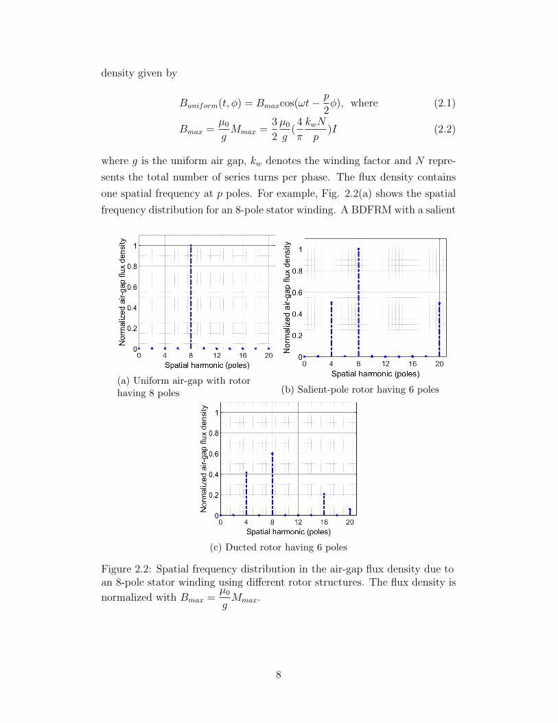
one spatial frequency at p poles. For example, Fig. 2.2(a) shows the spatial
frequency distribution for an 8-pole stator winding. A BDFRM with a salient
(a) Uniform air-gap with rotorhaving 8 poles (b) Salient-pole rotor having 6 poles
(c) Ducted rotor having 6 poles
Figure 2.2: Spatial frequency distribution in the air-gap flux density due toan 8-pole stator winding using different rotor structures. The flux density is
normalized with Bmax =µ0
gMmax.
8
pole rotor of pr pole introduces a non-uniform air gap g, modeled as
g−1(φ, t) =1
G(1 + cospr(φ− wrmt)) (2.3)
where φ is the mechanical air-gap angle, wrm is the rotor mechanical speed
and G is the mean air gap. The rotor modulation creates two side-bands in
the air-gap flux density along with the fundamental component by exciting
the primary stator having pp poles [19]. The air-gap flux density distribution
is given by
Bsalient = Bmaxcos(ωpt−pp2φ)
+Bmax
2cos[(ωp − prωrm)t− (
pp2− pr)φ)]
+Bmax
2cos[(ωp + prωrm)t− (
pp2
+ pr)φ)]
(2.4)
The secondary stator is constructed either with pr −pp2
pole-pair or pr +pp2
pole-pair to couple with the primary stator. For example, Fig 2.2(b)
shows the spatial frequency distribution for an 8-pole primary stator and
6-pole salient rotor. The secondary stator must be either 4 or 20 to produce
steady torque. The uncoupled side-band contributes only to the leakage
flux, resulting in poor efficiency, torque density and power factor compared
to uniform air-gap machines.
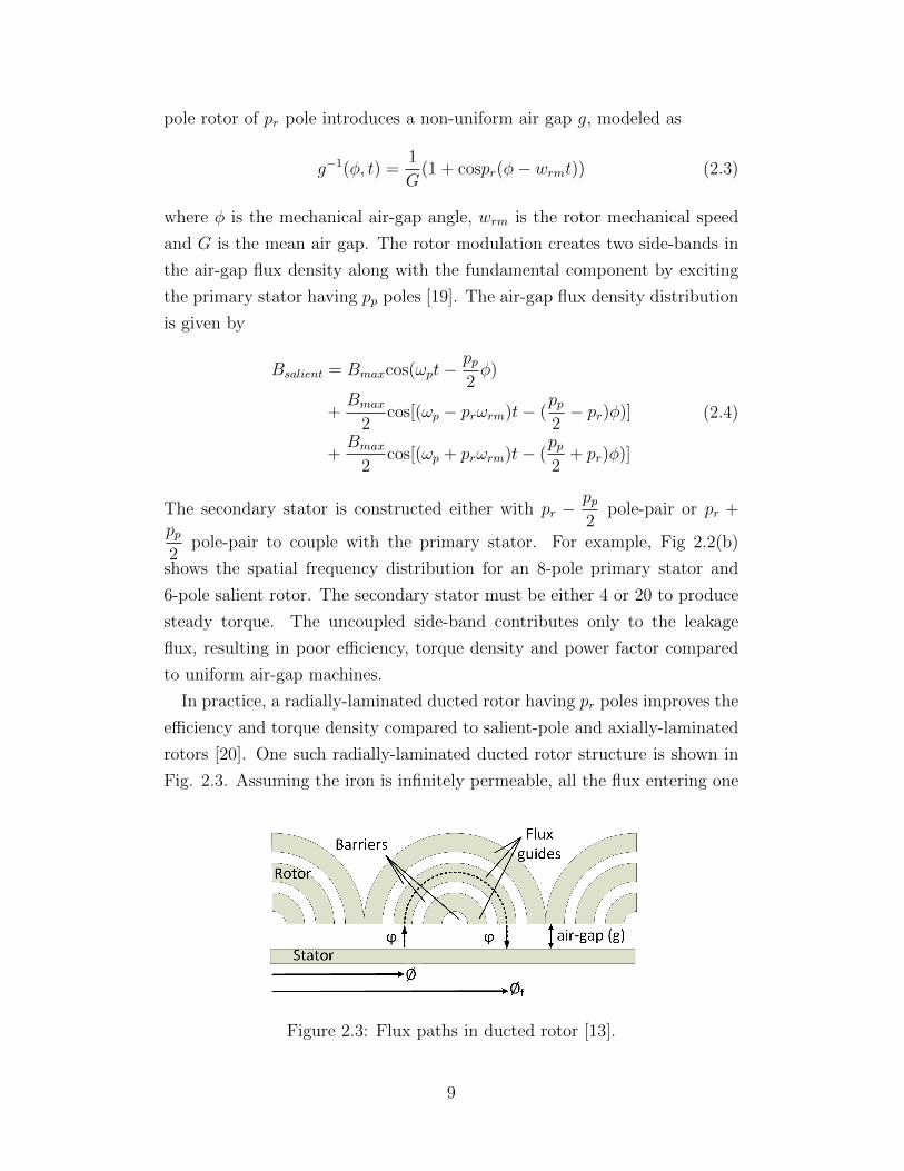
In practice, a radially-laminated ducted rotor having pr poles improves the
efficiency and torque density compared to salient-pole and axially-laminated
rotors [20]. One such radially-laminated ducted rotor structure is shown in
Fig. 2.3. Assuming the iron is infinitely permeable, all the flux entering one
Figure 2.3: Flux paths in ducted rotor [13].
9
of the rotor ducts at an air-gap angle of φ exits from the same duct at φf
[13], where
φf = φ+2π
pr− 2mod(φ,
2π
pr) (2.5)
The air-gap flux density due to the primary stator winding having pp poles
is
Bp(φ) =µ0Mp
g
1
2[cos(
pp2φ)− cos(
pp2φf )] (2.6)
Inherent non-linearity in φf introduces spatial harmonics in the air-gap flux
density. The flux density distribution is expanded as a Fourier series to give
Bp(φ) =∞∑i=1
Bpicos(iφ) =µ0Mp
g
∞∑i=1
Cpicos(iφ) (2.7)
where Cpi are the Fourier coefficients. Figure 2.2(c) shows the spatial fre-
quency distribution of the flux density for an 8-pole primary stator and a
6-pole ducted rotor. Comparison of Fig. 2.2(b) and 2.2(c) shows that in a
ducted-rotor, additional harmonic poles are generated that do not obey the
general formulation given by (2.4), which is valid for salient-pole rotors. For
the current example with 8-pole primary stator and a 6-pole rotor, the most
dominant sideband appears at 4 poles. Thus having a secondary stator of 4
poles will lead to maximum torque capability.
2.2 Machine inductances
This section computes the self and mutual inductances of the primary and
secondary stator windings. These inductances are used to model the machine
and compute the base-line torque produced by the interaction between the
primary and secondary stator in Chapter 3.
Using (2.7) and (2.2), the air-gap flux density with the primary stator
A-phase excited is given by
BpA =µ0
g
( 4
π
kwNp
pp
)Ip
∞∑i=1
Cpicos(iφ) (2.8)
Considering the winding function of primary stator A-phase wpa to be sinu-
10
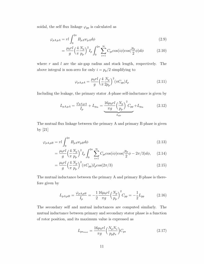
soidal, the self flux linkage ϕpp is calculated as
ϕpA,pA = rl
∫ 2π
0
BpAwpAdφ (2.9)
=µ0rl
g
( 4
π
Np
pp
)2Ip
∫ 2π
0
∞∑i=1
Cpicos(iφ)cos(pp2φ)dφ (2.10)
where r and l are the air-gap radius and stack length, respectively. The
above integral is non-zero for only i = pp/2 simplifying to
ϕpA,pA =µ0rl
g
( 4
π
Np
2pp
)2(πCpp)Ip (2.11)
Including the leakage, the primary stator A-phase self-inductance is given by
LpA,pA =ϕpA,pAIp
+ Lplk =16µ0rl
πg
(Np
pp
)2Cpp︸ ︷︷ ︸
Lpp
+Lplk (2.12)
The mutual flux linkage between the primary A and primary B phase is given
by [21]
ϕpA,pB = rl
∫ 2π
0
BpAwpBdφ (2.13)
=µ0rl
g
( 4
π
Np
pp
)2Ip
∫ 2π
0
∞∑i=1
Cpicos(iφ)cos(pp2φ− 2π/3)dφ, (2.14)
=µ0rl
g
( 4
π
Np
pp
)2(πCpp)Ipcos(2π/3) (2.15)
The mutual inductance between the primary A and primary B phase is there-
fore given by
LpA,pB =ϕpA,pBIp
= −1
2
16µ0rl
πg
(Np
pp
)2Cpp = −1
2Lpp (2.16)
The secondary self and mutual inductances are computed similarly. The
mutual inductance between primary and secondary stator phase is a function
of rotor position, and its maximum value is expressed as
Lpsmax =16µ0rl
πg
(NpNs
ppps
)Cps (2.17)
11
CHAPTER 3
DYNAMIC MODEL
This chapter discusses a generalized machine model for BDFRM, which will
be used to control the motor and to ascertain the size of the power electronic
converter. A conventional approach to modeling a machine incorporates
computation of variables such as currents, torque and speed for a given set of
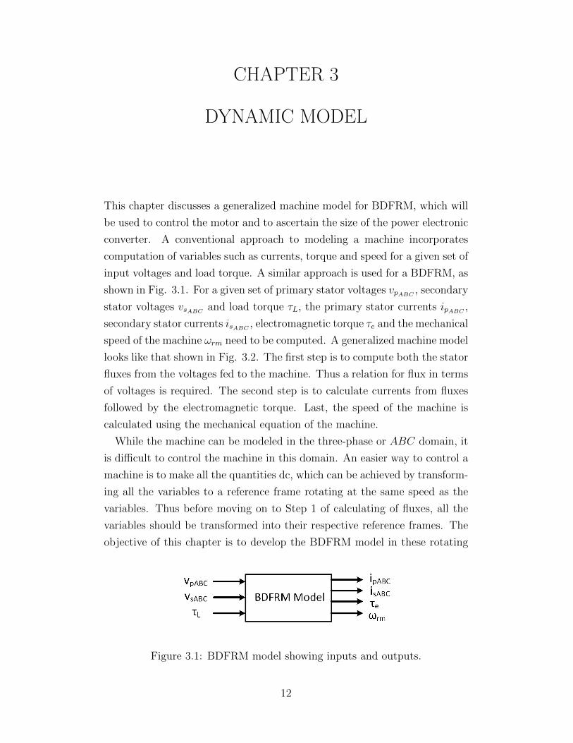
input voltages and load torque. A similar approach is used for a BDFRM, as
shown in Fig. 3.1. For a given set of primary stator voltages vpABC, secondary
stator voltages vsABCand load torque τL, the primary stator currents ipABC
,
secondary stator currents isABC, electromagnetic torque τe and the mechanical
speed of the machine ωrm need to be computed. A generalized machine model
looks like that shown in Fig. 3.2. The first step is to compute both the stator
fluxes from the voltages fed to the machine. Thus a relation for flux in terms
of voltages is required. The second step is to calculate currents from fluxes
followed by the electromagnetic torque. Last, the speed of the machine is
calculated using the mechanical equation of the machine.
While the machine can be modeled in the three-phase or ABC domain, it
is difficult to control the machine in this domain. An easier way to control a
machine is to make all the quantities dc, which can be achieved by transform-
ing all the variables to a reference frame rotating at the same speed as the
variables. Thus before moving on to Step 1 of calculating of fluxes, all the
variables should be transformed into their respective reference frames. The
objective of this chapter is to develop the BDFRM model in these rotating
Figure 3.1: BDFRM model showing inputs and outputs.
12
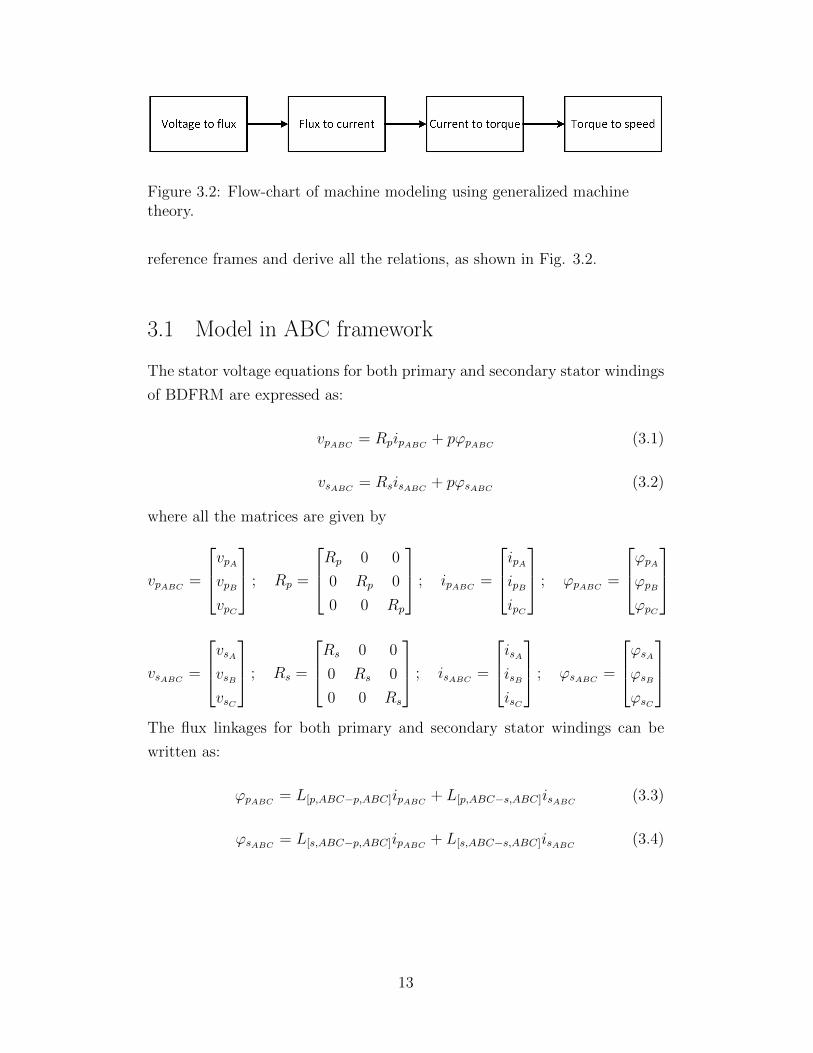
Figure 3.2: Flow-chart of machine modeling using generalized machinetheory.
reference frames and derive all the relations, as shown in Fig. 3.2.
3.1 Model in ABC framework
The stator voltage equations for both primary and secondary stator windings
of BDFRM are expressed as:
vpABC= RpipABC
+ pϕpABC(3.1)
vsABC= RsisABC
+ pϕsABC(3.2)
where all the matrices are given by
vpABC=
vpAvpBvpC
; Rp =
Rp 0 0
0 Rp 0
0 0 Rp
; ipABC=
ipAipBipC
; ϕpABC=
ϕpAϕpBϕpC
vsABC=
vsAvsBvsC
; Rs =
Rs 0 0
0 Rs 0
0 0 Rs
; isABC=
isAisBisC
; ϕsABC=
ϕsAϕsBϕsC
The flux linkages for both primary and secondary stator windings can be
written as:
ϕpABC= L[p,ABC−p,ABC]ipABC
+ L[p,ABC−s,ABC]isABC(3.3)
ϕsABC= L[s,ABC−p,ABC]ipABC
+ L[s,ABC−s,ABC]isABC(3.4)
13
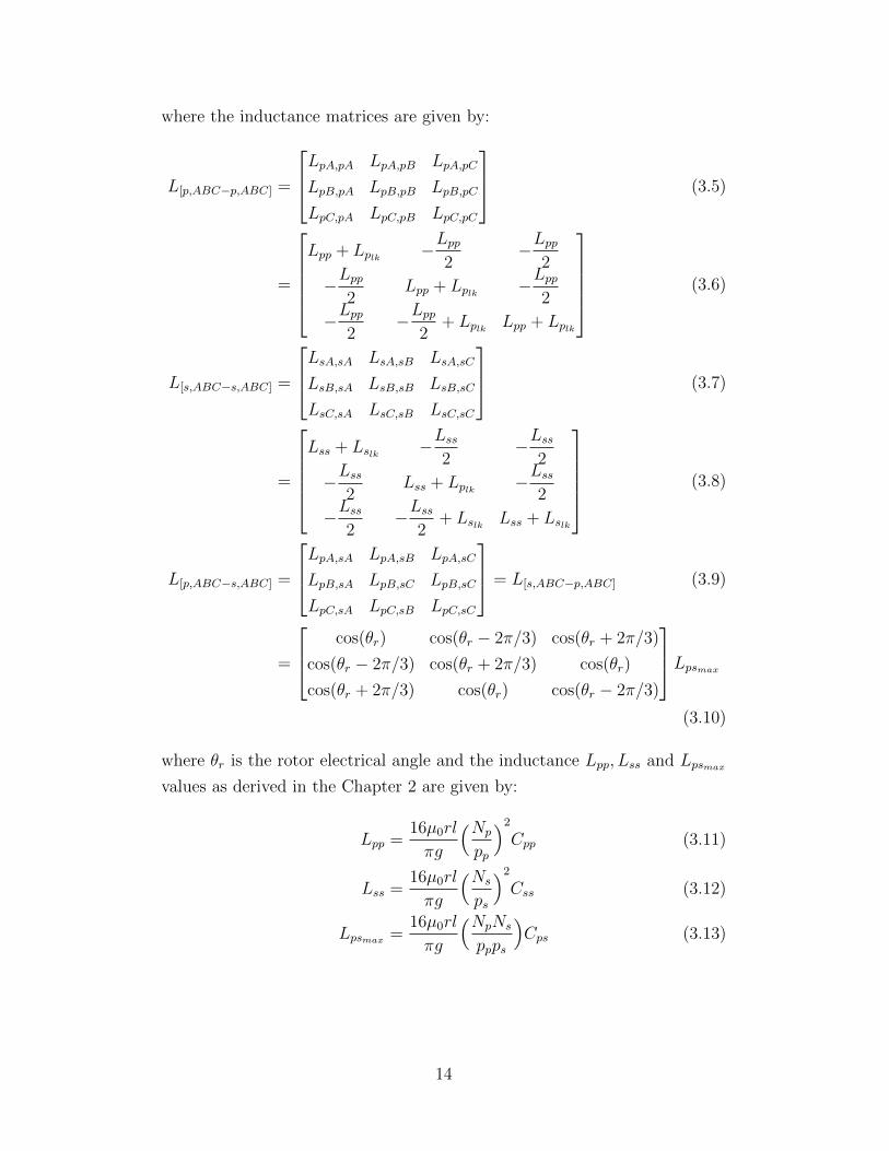
where the inductance matrices are given by:
L[p,ABC−p,ABC] =
LpA,pA LpA,pB LpA,pC
LpB,pA LpB,pB LpB,pC
LpC,pA LpC,pB LpC,pC
(3.5)
=
Lpp + Lplk −Lpp
2−Lpp
2
−Lpp2
Lpp + Lplk −Lpp2
−Lpp2
−Lpp2
+ Lplk Lpp + Lplk
(3.6)
L[s,ABC−s,ABC] =
LsA,sA LsA,sB LsA,sC
LsB,sA LsB,sB LsB,sC
LsC,sA LsC,sB LsC,sC
(3.7)
=
Lss + Lslk −Lss
2−Lss
2
−Lss2
Lss + Lplk −Lss2
−Lss2
−Lss2
+ Lslk Lss + Lslk
(3.8)
L[p,ABC−s,ABC] =
LpA,sA LpA,sB LpA,sC
LpB,sA LpB,sC LpB,sC
LpC,sA LpC,sB LpC,sC
= L[s,ABC−p,ABC] (3.9)
=
cos(θr) cos(θr − 2π/3) cos(θr + 2π/3)
cos(θr − 2π/3) cos(θr + 2π/3) cos(θr)
cos(θr + 2π/3) cos(θr) cos(θr − 2π/3)
Lpsmax
(3.10)
where θr is the rotor electrical angle and the inductance Lpp, Lss and Lpsmax
values as derived in the Chapter 2 are given by:
Lpp =16µ0rl
πg
(Np
pp
)2Cpp (3.11)
Lss =16µ0rl
πg
(Ns
ps
)2Css (3.12)
Lpsmax =16µ0rl
πg
(NpNs
ppps
)Cps (3.13)
14
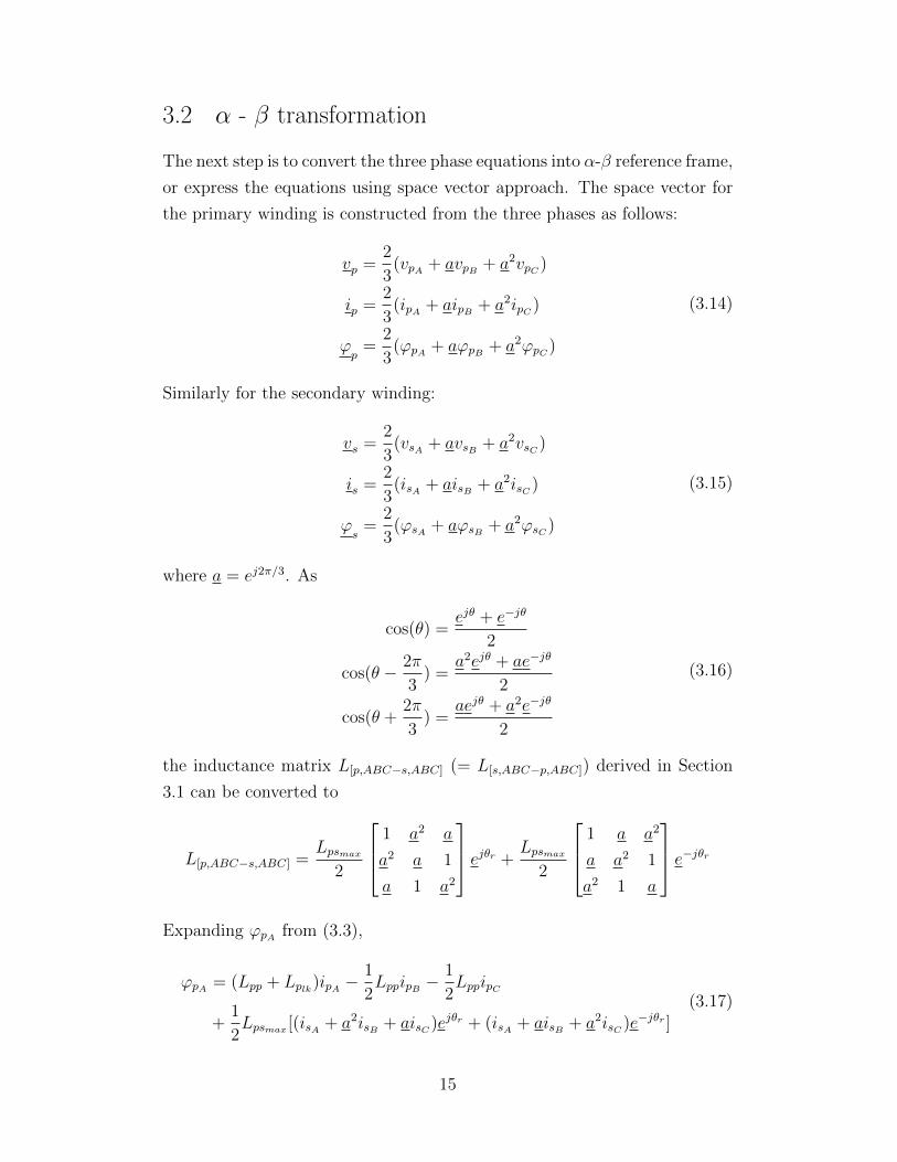
3.2 α - β transformation
The next step is to convert the three phase equations into α-β reference frame,
or express the equations using space vector approach. The space vector for
the primary winding is constructed from the three phases as follows:
vp =2
3(vpA + avpB + a2vpC )
ip =2
3(ipA + aipB + a2ipC )
ϕp
=2
3(ϕpA + aϕpB + a2ϕpC )
(3.14)
Similarly for the secondary winding:
vs =2
3(vsA + avsB + a2vsC )
is =2
3(isA + aisB + a2isC )
ϕs
=2
3(ϕsA + aϕsB + a2ϕsC )
(3.15)
where a = ej2π/3. As
cos(θ) =ejθ + e−jθ
2
cos(θ − 2π
3) =
a2ejθ + ae−jθ
2
cos(θ +2π
3) =
aejθ + a2e−jθ
2
(3.16)
the inductance matrix L[p,ABC−s,ABC] (= L[s,ABC−p,ABC]) derived in Section
3.1 can be converted to
L[p,ABC−s,ABC] =Lpsmax
2
1 a2 a
a2 a 1
a 1 a2
ejθr +Lpsmax
2
1 a a2
a a2 1
a2 1 a
e−jθrExpanding ϕpA from (3.3),
ϕpA = (Lpp + Lplk)ipA −1
2LppipB −
1
2LppipC
+1
2Lpsmax [(isA + a2isB + aisC )ejθr + (isA + aisB + a2isC )e−jθr ]
(3.17)
15
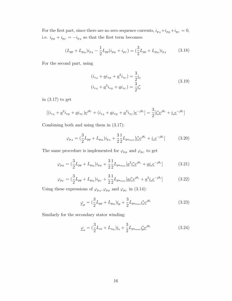
For the first part, since there are no zero sequence currents, ipA+ipB +ipC = 0,
i.e. ipB + ipC = −ipA so that the first term becomes:
(Lpp + Lplk)ipA −1
2Lpp(ipB + ipC ) = (
3
2Lpp + Lplk)ipA (3.18)
For the second part, using
(isA + aisB + a2isC ) =3
2is
(isA + a2isB + aisC ) =3
2i∗s
(3.19)
in (3.17) to get
[(isA + a2isB + aisC )ejθr + (isA + aisB + a2isC )e−jθr ] =3
2[i∗se
jθr + ise−jθr ]
Combining both and using them in (3.17):
ϕpA = (3
2Lpp + Lplk)ipA +
3
2
1
2Lpsmax [i∗se
jθr + ise−jθr ] (3.20)
The same procedure is implemented for ϕpB and ϕpC to get
ϕpB = (3
2Lpp + Lplk)ipB +
3
2
1
2Lpsmax [a2i∗se
jθr + aise−jθr ] (3.21)
ϕpC = (3
2Lpp + Lplk)ipC +
3
2
1
2Lpsmax [ai∗se
jθr + a2ise−jθr ] (3.22)
Using these expressions of ϕpA , ϕpB and ϕpC in (3.14):
ϕp
= (3
2Lpp + Lplk)ip +
3
2Lpsmaxi
∗sejθr (3.23)
Similarly for the secondary stator winding:
ϕs
= (3
2Lss + Lslk)is +
3
2Lpsmaxi
∗pejθr (3.24)
16
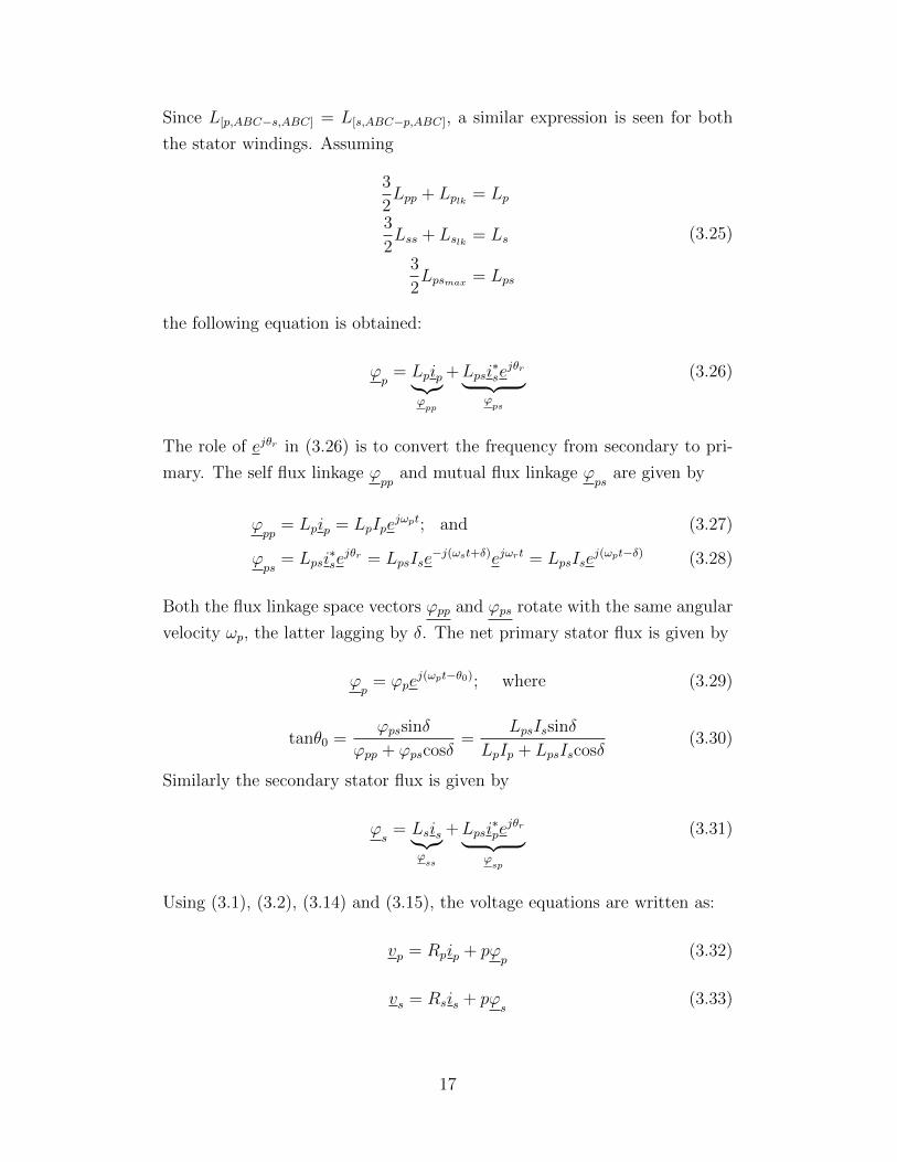
Since L[p,ABC−s,ABC] = L[s,ABC−p,ABC], a similar expression is seen for both
the stator windings. Assuming
3
2Lpp + Lplk = Lp
3
2Lss + Lslk = Ls
3
2Lpsmax = Lps
(3.25)
the following equation is obtained:
ϕp
= Lpip︸︷︷︸ϕpp
+Lpsi∗sejθr︸ ︷︷ ︸
ϕps
(3.26)
The role of ejθr in (3.26) is to convert the frequency from secondary to pri-
mary. The self flux linkage ϕpp
and mutual flux linkage ϕps
are given by
ϕpp
= Lpip = LpIpejωpt; and (3.27)
ϕps
= Lpsi∗sejθr = LpsIse
−j(ωst+δ)ejωrt = LpsIsej(ωpt−δ) (3.28)
Both the flux linkage space vectors ϕpp and ϕps rotate with the same angular
velocity ωp, the latter lagging by δ. The net primary stator flux is given by
ϕp
= ϕpej(ωpt−θ0); where (3.29)
tanθ0 =ϕpssinδ
ϕpp + ϕpscosδ=
LpsIssinδ
LpIp + LpsIscosδ(3.30)
Similarly the secondary stator flux is given by
ϕs
= Lsis︸︷︷︸ϕss
+Lpsi∗pejθr︸ ︷︷ ︸
ϕsp
(3.31)
Using (3.1), (3.2), (3.14) and (3.15), the voltage equations are written as:
vp = Rpip + pϕp
(3.32)
vs = Rsis + pϕs
(3.33)
17
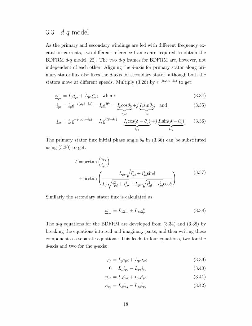
3.3 d-q model
As the primary and secondary windings are fed with different frequency ex-
citation currents, two different reference frames are required to obtain the
BDFRM d-q model [22]. The two d-q frames for BDFRM are, however, not
independent of each other. Aligning the d-axis for primary stator along pri-
mary stator flux also fixes the d-axis for secondary stator, although both the
stators move at different speeds. Multiply (3.26) by e−j(ωpt−θ0) to get:
ϕpr
= Lpipr + Lpsi∗sr; where (3.34)
ipr = ipe−j(ωpt−θ0) = Ipe
jθ0 = Ipcosθ0︸ ︷︷ ︸ipd
+j Ipsinθ0︸ ︷︷ ︸ipq
; and (3.35)
isr = ise−j(ωst+θ0) = Ise
j(δ−θ0) = Iscos(δ − θ0)︸ ︷︷ ︸isd
+j Issin(δ − θ0)︸ ︷︷ ︸isq
(3.36)
The primary stator flux initial phase angle θ0 in (3.36) can be substituted
using (3.30) to get:
δ = arctan( isqisd
)+ arctan
(Lps
√i2sd + i2sqsinδ
Lp√i2pd + i2pq + Lps
√i2sd + i2sqcosδ
) (3.37)
Similarly the secondary stator flux is calculated as
ϕsr
= Lsisr + Lpsi∗pr (3.38)
The d-q equations for the BDFRM are developed from (3.34) and (3.38) by
breaking the equations into real and imaginary parts, and then writing these
components as separate equations. This leads to four equations, two for the
d-axis and two for the q-axis:
ϕp = Lpipd + Lpsisd (3.39)
0 = Lpipq − Lpsisq (3.40)
ϕsd = Lsisd + Lpsipd (3.41)
ϕsq = Lsisq − Lpsipq (3.42)
18
since ϕpd = ϕp and ϕpq = 0 in primary stator flux reference frame. To get the
primary stator voltage equation in the primary stator flux reference frame,
multiply (3.32) by e−j(ωpt−θ0) to get:
vpr = Rpipr + pϕpr− ϕ
ppe−j(ωpt−θ0) (3.43)
= Rpipr + pϕpr
+ jωpϕpr (3.44)
Similarly the secondary stator voltage is calculated as
vsr = Rsisr + pϕsr
+ jωsϕsr (3.45)
The d-q voltage equations for the BDFRM are developed from (3.44) and
(3.45) by breaking the equations into real and imaginary parts, and then
writing these components as separate equations.
vpd = Rpipd + pϕp (3.46)
vpq = Rpipq + ωpϕp (3.47)
vsd = Rsisd + pϕsd − ωsϕsq (3.48)
vsq = Rsisq + pϕsq + ωsϕsd (3.49)
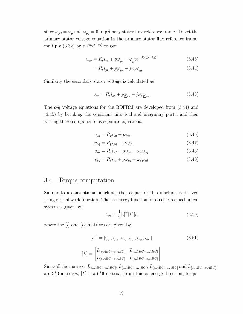
3.4 Torque computation
Similar to a conventional machine, the torque for this machine is derived
using virtual work function. The co-energy function for an electro-mechanical
system is given by:
Eco =1
2[i]T [L][i] (3.50)
where the [i] and [L] matrices are given by
[i]T = [ipA , ipB , ipC , isA , isB , isC ] (3.51)
[L] =
[L[p,ABC−p,ABC] L[p,ABC−s,ABC]
L[s,ABC−p,ABC] L[s,ABC−s,ABC]
]Since all the matrices L[p,ABC−p,ABC], L[s,ABC−s,ABC], L[p,ABC−s,ABC] and L[s,ABC−p,ABC]
are 3*3 matrices, [L] is a 6*6 matrix. From this co-energy function, torque
19
can be derived since
τe =∂Eco∂θrm
∣∣∣i=constant
= pr∂Eco∂θr
∣∣∣i=constant
(3.52)
Using the value of co-energy from (3.50),
τe =1
2pr[i]
T[ dLdθr
][i] (3.53)
Computation ofdL
dθrand torque τe is shown in Appendix A.1 and leads to
τe =1
2pr[i]
T[ dLdθr
][i] = j
3
4prLps[i
∗pri∗sr − iprisr] (3.54)
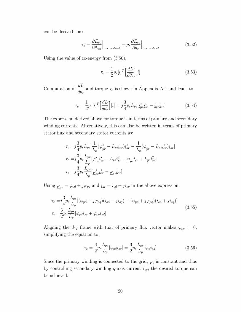
The expression derived above for torque is in terms of primary and secondary
winding currents. Alternatively, this can also be written in terms of primary
stator flux and secondary stator currents as:
τe =j3
4prLps[
1
Lp(ϕ∗
pr− Lpsisr)i∗sr −
1
Lp(ϕ
pr− Lpsi∗sr)isr]
τe =j3
4prLpsLp
[ϕ∗pri∗sr − Lpsi2sr − ϕprisr + Lpsi
2sr]
τe =j3
4prLpsLp
[ϕ∗pri∗sr − ϕprisr]
Using ϕpr
= ϕpd + jϕpq and isr = isd + jisq in the above expression:
τe =j3
4prLpsLp
[(ϕpd − jϕpq)(isd − jisq)− (ϕpd + jϕpq)(isd + jisq)]
τe =3
2prLpsLp
[ϕpdisq + ϕpqisd]
(3.55)
Aligning the d-q frame with that of primary flux vector makes ϕpq = 0,
simplifying the equation to:
τe =3
2prLpsLp
[ϕpdisq] =3
2prLpsLp
[ϕpisq] (3.56)
Since the primary winding is connected to the grid, ϕp is constant and thus
by controlling secondary winding q-axis current isq, the desired torque can
be achieved.
20
3.5 Speed computation
The final step is to compute the rotor speed. The mechanical rotor speed
ωrm is calculated using
τe − τL = Bωrm + Jdωrmdt
(3.57)
where
τe: Electromagnetic torque produced by the machine
τL: Load torque
B: Damping coefficient
J : Machine inertia constant
ωrm: Rotor mechanical speed
To get the rotor electrical speed ωr, multiply both sides of (3.57) by pr to
get
pr(τe − τL) = Bprωrm + Jprdωrmdt
pr(τe − τL) = Bωr + Jdωrdt
(3.58)
21
CHAPTER 4
DRIVE CONTROL ARCHITECTURE
Various control methodologies have been investigated for the BDFRM, in-
cluding scalar control [23], [24], field-oriented control (FOC) [24, 25, 26], and
direct torque control (DTC) [27]. The conventional FOC approach, as shown
in Fig. 4.1, has been used for this study. The machine d-q model developed
in Chapter 3 will be used to develop the necessary control of secondary stator
through a drive end converter. Since the machine model is based on primary
stator flux reference frame, the calculation of the magnitude and phase angle
of primary stator flux is done first. This flux angle along with the rotor an-
gle is used to transform secondary stator variables into d-q reference frame,
required by the two current controllers. The design of both the secondary
stator current controllers is discussed next followed by the speed and reactive
power controllers.
4.1 Stator flux estimation
The primary stator flux ϕp along with the flux angle θp (with respect to
primary stator A-phase axis) and flux frequency wp are estimated using the
measured values of ac source voltage vp and current ip connected to three
phases of the primary stator. The computed primary stator flux angle is
used to transform the variables to primary stator flux reference frame. Using
(3.32), the primary stator flux space vector is given by
ϕp
=
∫(vp −Rpip)dt (4.1)
For practical implementation, the integrator is replaced by a low-pass filter
with a suitable time-constant to avoid problems with measurement offset and
drift in the integral computations [28]. The cutoff frequency of these low-pass
22
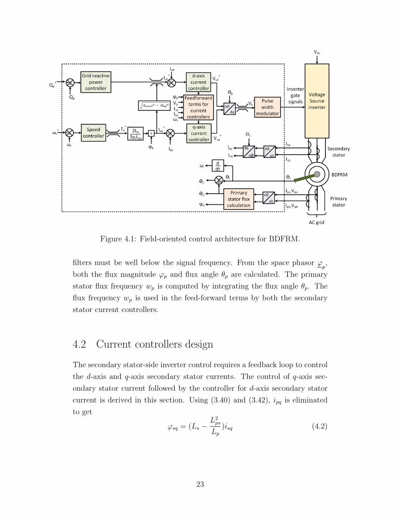
Figure 4.1: Field-oriented control architecture for BDFRM.
filters must be well below the signal frequency. From the space phasor ϕp,
both the flux magnitude ϕp and flux angle θp are calculated. The primary
stator flux frequency wp is computed by integrating the flux angle θp. The
flux frequency wp is used in the feed-forward terms by both the secondary
stator current controllers.
4.2 Current controllers design
The secondary stator-side inverter control requires a feedback loop to control
the d-axis and q-axis secondary stator currents. The control of q-axis sec-
ondary stator current followed by the controller for d-axis secondary stator
current is derived in this section. Using (3.40) and (3.42), ipq is eliminated
to get
ϕsq = (Ls −L2ps
Lp)isq (4.2)
23
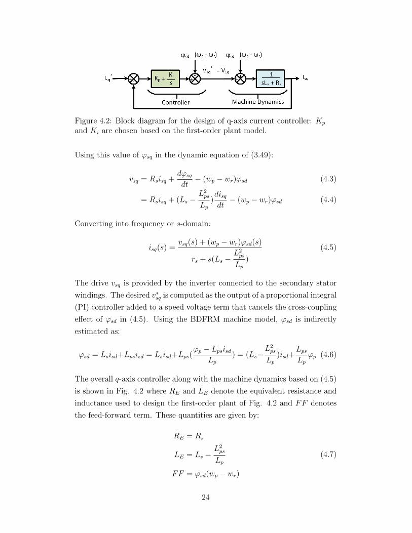
Figure 4.2: Block diagram for the design of q-axis current controller: Kp
and Ki are chosen based on the first-order plant model.
Using this value of ϕsq in the dynamic equation of (3.49):
vsq = Rsisq +dϕsqdt− (wp − wr)ϕsd (4.3)
= Rsisq + (Ls −L2ps
Lp)disqdt− (wp − wr)ϕsd (4.4)
Converting into frequency or s-domain:
isq(s) =vsq(s) + (wp − wr)ϕsd(s)
rs + s(Ls −L2ps
Lp)
(4.5)
The drive vsq is provided by the inverter connected to the secondary stator
windings. The desired v∗sq is computed as the output of a proportional integral
(PI) controller added to a speed voltage term that cancels the cross-coupling
effect of ϕsd in (4.5). Using the BDFRM machine model, ϕsd is indirectly
estimated as:
ϕsd = Lsisd+Lpsisd = Lsisd+Lps(ϕp − Lpsisd
Lp) = (Ls−
L2ps
Lp)isd+
LpsLp
ϕp (4.6)
The overall q-axis controller along with the machine dynamics based on (4.5)
is shown in Fig. 4.2 where RE and LE denote the equivalent resistance and
inductance used to design the first-order plant of Fig. 4.2 and FF denotes
the feed-forward term. These quantities are given by:
RE = Rs
LE = Ls −L2ps
Lp
FF = ϕsd(wp − wr)
(4.7)
24
Proportional and integral gains (Kp and Ki) of the controller are chosen to
ensure loop stability, desired transient response, and acceptable steady-state
error. The determination of Kp and Ki based on the first-order closed loop
system is derived in Appendix A.2
The design of the d-axis current controller is similar. Using (3.39) and
(3.41),
ϕsd = (Ls −L2ps
Lp)isd +
LpsLp
ϕp (4.8)
Using this value of ϕsd equation in (3.48),
vsd = Rsisd+dϕsddt
+(wp−wr)ϕsq = Rsisd+d
dt[(Ls−
L2ps
Lp)isd+
LpsLp
ϕp]+(wp−wr)ϕsq(4.9)
Using (4.2) to equate ϕsq in (4.9),
vsd = Rsisd +d
dt[(Ls −
L2ps
Lp)isd +
LpsLp
ϕp] + (wp − wr)(Ls −L2ps
Lp)isq (4.10)
vsd = Rsisd + (Ls −L2ps
Lp)disddt
+LpsLp
dϕpdt
+ (wp − wr)(Ls −L2ps
Lp)isq (4.11)
Also the rate of change of primary fluxdϕpdt
is expressed using (3.46) and
(3.39) as:
dϕpdt
= vpd −Rpipd
= vpd −Rp(ϕp − Lpsisd
Lp)
(4.12)
Using this value in (4.11),
vsd = (Rs+Rp
L2ps
L2p
)isd+(Ls−L2ps
Lp)disddt
+LpsLp
vpd−RpLpsL2p
ϕp+(wp−wr)(Ls−L2ps
Lp)isq
(4.13)
The equivalent inductance and resistance of the machine dynamics are ap-
propriately changed in Fig. 4.2 using (4.13) to design Kp and Ki for the PI
25
controller by making
RE = Rs +Rp
L2ps
L2p
LE = Ls −L2ps
Lp
FF =LpsLp
vpd −RpLpsL2p
ϕp + (wp − wr)(Ls −L2ps
Lp)isq
(4.14)
4.3 Speed controller
Using the rotor speed equation derived earlier in (3.58),
wr =pr(τe − τL)
B + sJ=
τe − τLB
pr+ s
J
pr
(4.15)
Since the drive torque is related to q-axis secondary stator current by (3.56)
τe =3
2prLpsLp
ϕpisq (4.16)
the reference q-axis secondary stator current is given by
i∗sq =τ ∗e
3
2prLpsLp
ϕp
=2
3
LpprLps
τ ∗e1
ϕp(4.17)
The overall control loop including both the speed and q-axis current controller
is determined and is shown in Fig. 4.3. The bandwidth of the speed controller
is chosen to be much smaller than that of the q-axis current controller. This
is a design choice that will determine the final performance of the propulsion
drive.
4.4 Reactive power controller
While the motor torque is controlled by the converter q-axis current, the
converter d-axis current is commanded to control the flow of primary stator
reactive power to and from the ac grid. The objective is to maintain the
26

Figure 4.3: The speed-control forms an outer control loop with the q-axissecondary stator current control inside it.
maximum possible power factor on the ac grid connected to the primary
stator. The primary stator reactive power is given by [19]:
Qp =3
2(vpqipd − vpdipq) =
3
2wpϕp(
ϕp − xpsisdxp
) (4.18)
This can be made zero, thus having a unity power factor on the ac grid, by
having
i∗sd =ϕpxps
(4.19)
This calculated reference d-axis current must also be less than the maximum
allowable value given by
i∗sdmax=√I2srated − i∗sq
2 (4.20)
The reference d-axis secondary stator current is hence given by
i∗sd = min(ϕpxps
,√I2srated − i∗sq
2) (4.21)
Just like the speed controller, the bandwidth of the reactive power controller
is chosen such that it is around one tenth that of the d-axis current controller.
27
CHAPTER 5
ELECTROMAGNETIC DESIGNMETHODOLOGY
This chapter discusses the electromagnetic design methodology of a BDFRM
for a TeDP system. The volumetric D2l sizing equation is derived. As the
design of BDFRM is unconventional, the design equation D2l is subsequently
transformed to a Dl sizing equation. The machine specifications and design
constraints are presented in Section 5.3.
5.1 D2l sizing derivation
The torque produced by a machine is proportional to the product of elec-
trical and magnetic loadings. The electrical loading is limited by the i2R
loss in the conductor, effectiveness of the cooling media, and the allowable
temperature rise in the insulating material. The magnetic loading is limited
by the saturation point of the material, and hysteresis and eddy current loss.
Therefore, the torque has an upper bound for a given amount of copper and
iron.
The basic design equations of a BDFRM having an ideal circular ducted
rotor are presented in [13]. The induced peak phase voltage (Ep) and peak
phase current (Ip) in the primary stator winding are given by
Ep = (lD)kwpNp2wppp
Bpp (5.1)
Ip =πD
6kwpNp
Ap (5.2)
where Bpp and Ap represent peak flux density and peak electric loading of
the primary stator winding with pp poles, respectively. Using (5.1) and (5.2),
28
output power from the primary stator is calculated by
Pp =3
2EpIpcosφpη = π(D2l)
wppp
ApBpp
2cosφpη (5.3)
Similarly, the output power from the secondary stator is
Ps = π(D2l)wsps
AsBps
2cosφsη = π(D2l)
(αwp)
ps
AsBs
2cosφsη (5.4)
where α = ws/wp is the frequency ratio of the secondary stator current to
the primary current. The mechanical output power of the machine is
Prated = PP + Ps = π(D2l)wp2
[ApBp
ppcosφp + α
AsBs
pscosφs
]η (5.5)
The secondary stator parameters Bs, As and cosφs are expressed in terms
of primary stator parameters Bp, Ap and cosφp to simplify (5.5). The peak
MMF produced by the primary stator winding Mp, when excited by current
of amplitude Ip, is given by
Mp =D
ppAp =
6
π
NpKwp
ppIp (5.6)
As derived in (2.7), the air-gap flux density due to this primary stator MMF
consists of several spatial harmonics, and is given by:
Bp(φ) =∞∑i=1
Bpicos(iφ) =µ0Mp
g
∞∑i=1
Cpiksatcos(iφ) (5.7)
where ksat accounts for the MMF drop in the iron. The spatial harmonic at
pp poles and ps poles are given by
Bpp = Cppksatµ0Mp
g(5.8)
Bsp = Cspksatµ0Mp
g(5.9)
Similarly, the peak MMF produced by the secondary stator winding Ms, and
the air-gap flux density produced by the secondary stator winding, when
excited by current of amplitude Is, with an initial phase offset δ, are given
29
by
Ms =D
psAs =
6
π
NsKws
psIs (5.10)
Bs(φ) =∞∑i=1
Bsicos(iφ− δ) =µ0Ms
g
∞∑i=1
Csiksatcos(iφ− δ) (5.11)
The spatial harmonics at pp poles and ps poles are given by
Bps = Cpsksatµ0Ms
g(5.12)
Bss = Cssksatµ0Ms
g(5.13)
The term δ in Bs is due to the phase difference in the excitation currents
between primary and secondary stator currents. δ = π/2 ensures a maximum
electromagnetic torque [29]. Therefore, peak magnitude of the primary stator
flux density (spatial harmonic pp poles) and secondary stator flux density
(spatial harmonic ps poles) are given by
Bpp =√Bpp
2 +Bps2 =
µ0ksatg
√(CppMp)2 + (CpsMs)2 (5.14)
Bps =√Bss
2 +Bsp2 =
µ0ksatg
√(CssMs)2 + (CspMp)2 (5.15)
As and Ms are also expressed in terms of Ap and Mp, respectively, using
(5.2), (5.6) and (5.10), as
As =kws
kwp
Ns
Np
IsIpAp (5.16)
Ms =ppps
AsApMp (5.17)
Reference [13] also discusses the computation of primary and secondary wind-
ing power factors as
tanφp =pspp
CppCps
ApAs
(5.18)
tanφs =ppps
CssCsp
AsAp
(5.19)
The extent of coupling between the two stator windings, denoted by the cou-
pling factors, plays a major role in sizing of the BDFRM. These depend upon
30
the pole combination of both the stators and the rotor. A pole combination
of pp = 8, ps = 4 and pr = 6 is chosen. Using these pole values, the coupling
factors are
Cpp = 0.6034, Csp = Cps = 0.4135, Css = 0.2935 (5.20)
For the initial machine design, the primary and secondary stator currents
and turns per phase are considered equal. Using Eqs. (5.16) and (5.17),
Ap ≈ As (5.21)
Ms ≈ 2Mp (5.22)
Using the coupling factors (Eq. (5.20)) and peak MMF (Eq. (5.22)) in Eqs.
(5.14) and (5.15), peak magnitude of the primary stator flux density Bpp and
secondary stator flux density Bps are given by
Bpp = 1.0237ksatµ0Mp
g(5.23)
Bps = 0.717ksatµ0Mp
g= 0.7Bpp (5.24)
The shear stress for both windings is
σp =BppAp
2(5.25)
σs =BpsAs
2= 0.7σp (5.26)
σnet = σp + σs = 1.7σp (5.27)
The net or rated power for the chosen pole combination is computed by
substituting (5.16) – (5.27) in (5.5) as
Prated = 0.125π(1 + α)wpσpcosφpη(D2l) = 0.88π2
60Nratedσnetcosφpη(D2l)
(5.28)
where Nrated is the rated rotor speed. The D2l equation for the selected pole
combination is given by
D2l =Prated
0.88π2
60Nratedσnetcosφpη
(5.29)
31
The D2l equation in (5.29) can be used as an initial sizing estimate of BD-
FRM, similar to a conventional machine. The shear stress is estimated to
be around 20-35 kPa for aerospace applications [30]. However, the machine
shear stress given by Eq. (5.27) should be re-evaluated for BDFRM to ensure
that such high shear stress does not force the iron into saturation. While the
D2l sizing equation is very useful for initial sizing of conventional machines,
this is not meaningful for BDFRM due to the dependency of magnetic and
electrical loadings. Therefore, a more useful Dl sizing equation is derived in
Section 5.2 and is used for initial sizing in Section 5.3.
5.2 Dl sizing derivation
Shear stress is computed in terms of design parameters and Bairgappeak , which
is chosen according to the core material saturation flux density. Using (2.5)
and (2.6), the air-gap flux density due to primary and secondary stator for
the chosen pole-combination is given by
Bp(φ) =µ0Mp
2g
[cos4φ− cos4
(φ+
π
3− 2mod(φ,
π
3))]
(5.30)
Bs(φ) =µ0Ms
2g
[cos(
2φ+π
2
)− cos
(2(φ+
π
3− 2mod(φ,
π
3))
+π
2
)](5.31)
Figure 5.1 shows both the normalized flux densities Bp, Bs along with the
net flux density in the air-gap with Ms = 2Mp, as discussed earlier in Section
5.1. The peak air-gap flux density, as observed from this figure is
Bairgappeak = 3.45µ0Mp
2g= 1.725
µ0Mp
g(5.32)
Using (5.6), (5.32) and (5.27), the net shear stress is expressed as
σnet = 1.7σp = 1.7BppAp
2= 2.34
ksatµ0
g
DB2airgappeak
(5.33)
32
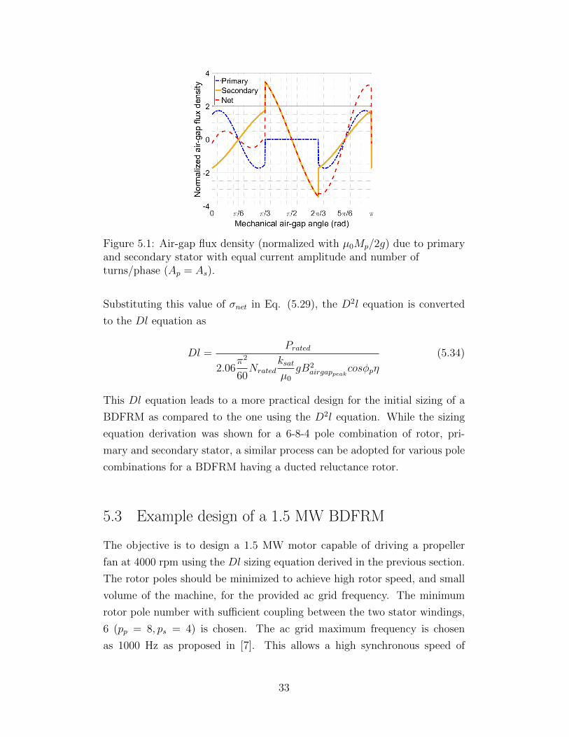
Figure 5.1: Air-gap flux density (normalized with µ0Mp/2g) due to primaryand secondary stator with equal current amplitude and number ofturns/phase (Ap = As).
Substituting this value of σnet in Eq. (5.29), the D2l equation is converted
to the Dl equation as
Dl =Prated
2.06π2
60Nrated
ksatµ0
gB2airgappeak
cosφpη
(5.34)
This Dl equation leads to a more practical design for the initial sizing of a
BDFRM as compared to the one using the D2l equation. While the sizing
equation derivation was shown for a 6-8-4 pole combination of rotor, pri-
mary and secondary stator, a similar process can be adopted for various pole
combinations for a BDFRM having a ducted reluctance rotor.
5.3 Example design of a 1.5 MW BDFRM
The objective is to design a 1.5 MW motor capable of driving a propeller
fan at 4000 rpm using the Dl sizing equation derived in the previous section.
The rotor poles should be minimized to achieve high rotor speed, and small
volume of the machine, for the provided ac grid frequency. The minimum
rotor pole number with sufficient coupling between the two stator windings,
6 (pp = 8, ps = 4) is chosen. The ac grid maximum frequency is chosen
as 1000 Hz as proposed in [7]. This allows a high synchronous speed of
33
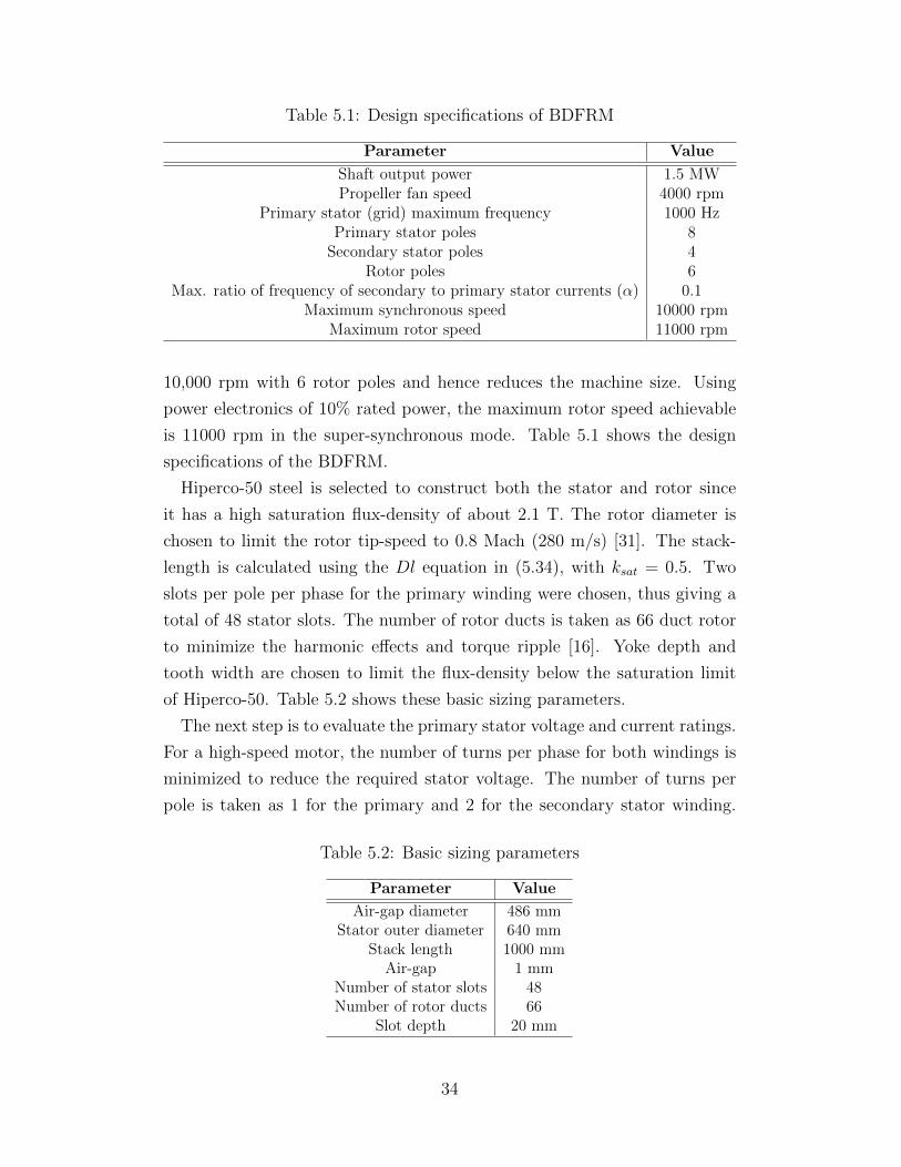
Table 5.1: Design specifications of BDFRM
Parameter Value
Shaft output power 1.5 MWPropeller fan speed 4000 rpm
Primary stator (grid) maximum frequency 1000 HzPrimary stator poles 8
Secondary stator poles 4Rotor poles 6
Max. ratio of frequency of secondary to primary stator currents (α) 0.1Maximum synchronous speed 10000 rpm
Maximum rotor speed 11000 rpm
10,000 rpm with 6 rotor poles and hence reduces the machine size. Using
power electronics of 10% rated power, the maximum rotor speed achievable
is 11000 rpm in the super-synchronous mode. Table 5.1 shows the design
specifications of the BDFRM.
Hiperco-50 steel is selected to construct both the stator and rotor since
it has a high saturation flux-density of about 2.1 T. The rotor diameter is
chosen to limit the rotor tip-speed to 0.8 Mach (280 m/s) [31]. The stack-
length is calculated using the Dl equation in (5.34), with ksat = 0.5. Two
slots per pole per phase for the primary winding were chosen, thus giving a
total of 48 stator slots. The number of rotor ducts is taken as 66 duct rotor
to minimize the harmonic effects and torque ripple [16]. Yoke depth and
tooth width are chosen to limit the flux-density below the saturation limit
of Hiperco-50. Table 5.2 shows these basic sizing parameters.
The next step is to evaluate the primary stator voltage and current ratings.
For a high-speed motor, the number of turns per phase for both windings is
minimized to reduce the required stator voltage. The number of turns per
pole is taken as 1 for the primary and 2 for the secondary stator winding.
Table 5.2: Basic sizing parameters
Parameter Value
Air-gap diameter 486 mmStator outer diameter 640 mm
Stack length 1000 mmAir-gap 1 mm
Number of stator slots 48Number of rotor ducts 66
Slot depth 20 mm
34

This gives a total of 8 turns per phase for both stator windings. Equations
(5.21) and (5.32) are then used to compute the current rating for both stator
windings. Neglecting the resistances, (5.1) and (5.23) are used to determine
the primary stator voltage rating. Table 5.3 shows the calculated motor
ratings following the FEA validation of analytical design equations. The
conventional approach to designing BDFRM leads to low shear stress and
low torque density. Chapter 6 discusses an approach to improving the torque
density in this machine.
Table 5.3: Motor ratings
Parameter Value
Primary stator phase voltage 4 kV peakPrimary and secondary stator phase current 300 A peakPrimary and secondary stator turns/phase 8
Primary winding power factor 0.8Net Shear stress 4.6 kPa
Efficiency 97.6%
35
CHAPTER 6
TORQUE DENSITY IMPROVEMENT
The torque density of the designed 1.5 MW BDFRM is poor, as seen in
Chapter 5. The conventional approach of having equal electric loading on
both stator windings is not appropriate since the stators have different pole
numbers. As will be seen in this chapter, the choice of initial phase offset
δ being π/2 also is not an optimum value for maximum torque production.
An optimization problem is formulated to maximize torque density, with the
two electric loadings and the phase offset δ as the design variables. The
flux density, current density, machine dimensions and primary stator voltage
rating are chosen as constraints.
In order to express air-gap flux density due to primary stator Bp in terms
of its peak specific electric loading Ap, the relationship between Mp and Ap
is used. This leads to the following equation using (2.6):
Bp(φ) =1
2
[cos
pp2φ− cos
pp2φf
]µ0DApgpp
(6.1)
Similarly, the secondary stator winding with ps poles excited using currents
of amplitude Is and an initial phase shift δ results in an air-gap flux density
given by
Bs(φ) =1
2
[cos(ps
2φ− δ
)− cos
(ps2φf − δ
)]µ0DAsgps
(6.2)
Torque in the synchronous operation mode is given by
Te =µ0lD
3
2g
prppps
CpsApAssinδ (6.3)
The peak primary current density is expressed in terms of peak electrical
loadings as:
Jp =τsApfαAslot
(6.4)
36
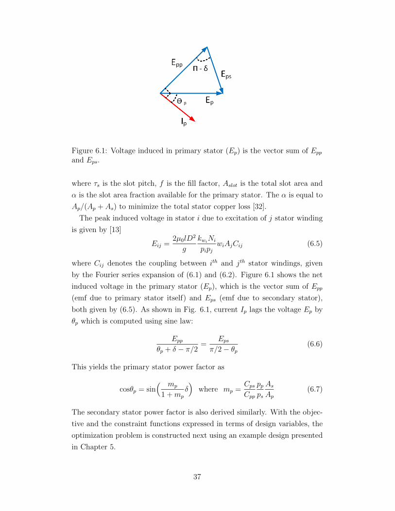
Figure 6.1: Voltage induced in primary stator (Ep) is the vector sum of Eppand Eps.
where τs is the slot pitch, f is the fill factor, Aslot is the total slot area and
α is the slot area fraction available for the primary stator. The α is equal to
Ap/(Ap + As) to minimize the total stator copper loss [32].
The peak induced voltage in stator i due to excitation of j stator winding
is given by [13]
Eij =2µ0lD
2
g
kwiNi
pipjwiAjCij (6.5)
where Cij denotes the coupling between ith and jth stator windings, given
by the Fourier series expansion of (6.1) and (6.2). Figure 6.1 shows the net
induced voltage in the primary stator (Ep), which is the vector sum of Epp
(emf due to primary stator itself) and Eps (emf due to secondary stator),
both given by (6.5). As shown in Fig. 6.1, current Ip lags the voltage Ep by
θp which is computed using sine law:
Eppθp + δ − π/2
=Eps
π/2− θp(6.6)
This yields the primary stator power factor as
cosθp = sin( mp
1 +mp
δ)
where mp =CpsCpp
ppps
AsAp
(6.7)
The secondary stator power factor is also derived similarly. With the objec-
tive and the constraint functions expressed in terms of design variables, the
optimization problem is constructed next using an example design presented
in Chapter 5.
37
6.1 Optimization problem formulation
The objective is to maximize torque under the flux and current-density con-
straints without modifying the machine's physical dimensions. The optimiza-
tion problem is set up as [14]:
maximizeAp,As, δ
Te = keApAssinδ; ke =µ0lD
3
2g
prppps
Cps
subject to |∑i=p,s
Ji| ≤ Jmax,
|Bi(φ)| ≤ Bmax; i = p, s,
|Bnet(φ)| = |∑i=p,s
Bi(φ)| ≤ Bmax
(6.8)
The conventional FEA optimization solver is time consuming. The motor's
properties are examined here analytically so that the optimization is solved
using a time-saving tool like MATLAB. Instead of applying the flux den-
sity constraints in the iron core, these constraints are applied only along the
air gap. The maximum flux density in stator tooth and rotor ducts is ap-
proximately 1.7 times the maximum air-gap flux density Bmax [33]. Bmax is
chosen based on the material saturation flux density. Even at the air gap,
the optimization problem is quite challenging to solve due to the time- and
space-varying nature of flux density. Therefore, constraints are applied only
at t = 0 s since the amplitude of Bnet waveform remains nearly constant, i.e.,
independent of rotor position [29]. To avoid the space variation along the air
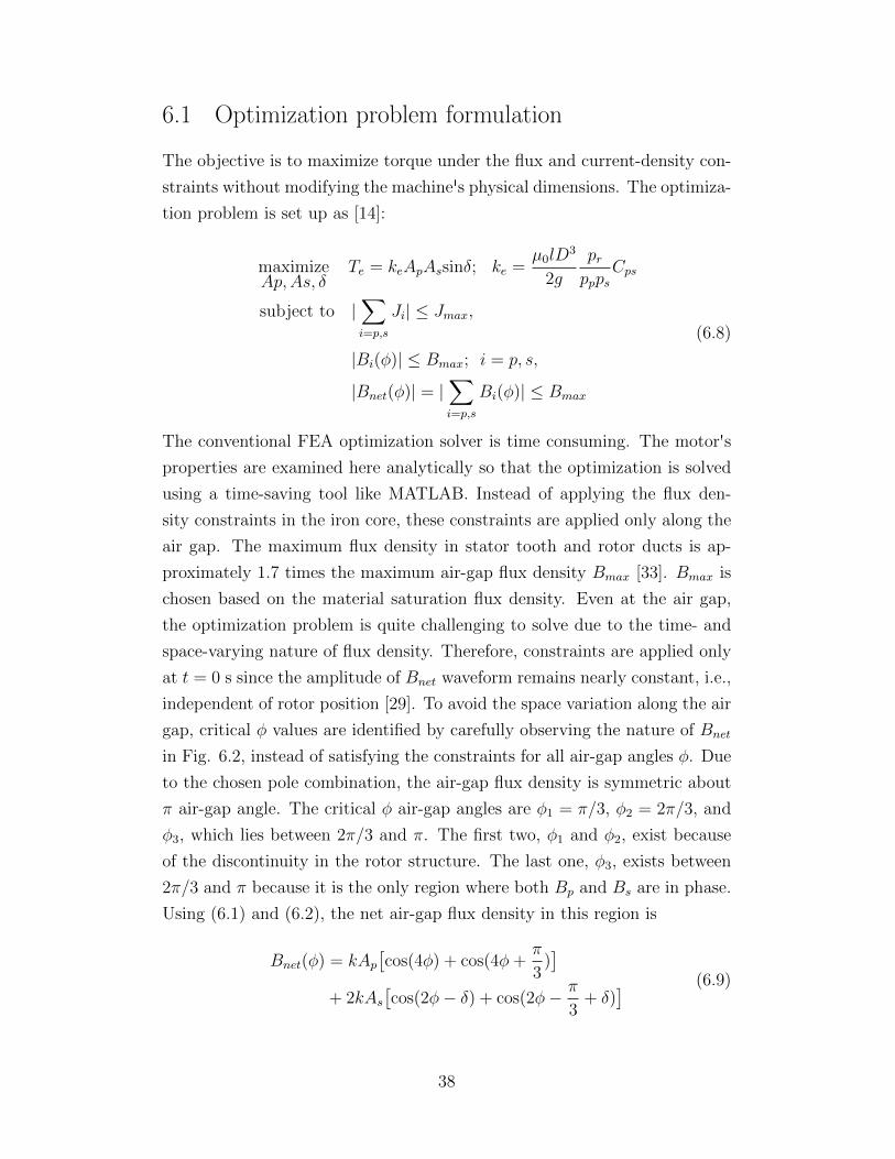
gap, critical φ values are identified by carefully observing the nature of Bnet
in Fig. 6.2, instead of satisfying the constraints for all air-gap angles φ. Due
to the chosen pole combination, the air-gap flux density is symmetric about
π air-gap angle. The critical φ air-gap angles are φ1 = π/3, φ2 = 2π/3, and
φ3, which lies between 2π/3 and π. The first two, φ1 and φ2, exist because
of the discontinuity in the rotor structure. The last one, φ3, exists between
2π/3 and π because it is the only region where both Bp and Bs are in phase.
Using (6.1) and (6.2), the net air-gap flux density in this region is
Bnet(φ) = kAp[cos(4φ) + cos(4φ+
π
3)]
+ 2kAs[cos(2φ− δ) + cos(2φ− π
3+ δ)
] (6.9)
38
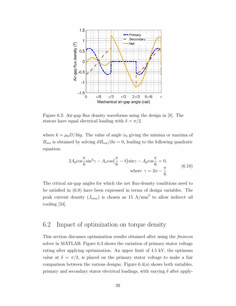
Figure 6.2: Air-gap flux density waveforms using the design in [8]. Thestators have equal electrical loading with δ = π/2.
where k = µ0D/16g. The value of angle φ3 giving the minima or maxima of
Bnet is obtained by solving ∂Bnet/∂φ = 0, leading to the following quadratic
equation:
2Apcosπ
6sin2γ − Ascos
(π6− δ)sinγ − Apcos
π
6= 0,
where γ = 2φ− π
6
(6.10)
The critical air-gap angles for which the net flux-density conditions need to
be satisfied in (6.8) have been expressed in terms of design variables. The
peak current density (Jmax) is chosen as 15 A/mm2 to allow indirect oil
cooling [34].
6.2 Impact of optimization on torque density
This section discusses optimization results obtained after using the fmincon
solver in MATLAB. Figure 6.3 shows the variation of primary stator voltage
rating after applying optimization. An upper limit of 4.5 kV, the optimum
value at δ = π/2, is placed on the primary stator voltage to make a fair
comparison between the various designs. Figure 6.4(a) shows both variables,
primary and secondary stator electrical loadings, with varying δ after apply-
39
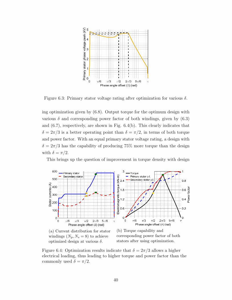
Figure 6.3: Primary stator voltage rating after optimization for various δ.
ing optimization given by (6.8). Output torque for the optimum design with
various δ and corresponding power factor of both windings, given by (6.3)
and (6.7), respectively, are shown in Fig. 6.4(b). This clearly indicates that
δ = 2π/3 is a better operating point than δ = π/2, in terms of both torque
and power factor. With an equal primary stator voltage rating, a design with
δ = 2π/3 has the capability of producing 75% more torque than the design
with δ = π/2.
This brings up the question of improvement in torque density with design
(a) Current distribution for statorwindings (Np, Ns = 8) to achieveoptimized design at various δ.
(b) Torque capability andcorresponding power factor of bothstators after using optimization.
Figure 6.4: Optimization results indicate that δ = 2π/3 allows a higherelectrical loading, thus leading to higher torque and power factor than thecommonly used δ = π/2.
40
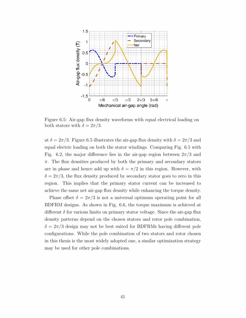
Figure 6.5: Air-gap flux density waveforms with equal electrical loading onboth stators with δ = 2π/3.
at δ = 2π/3. Figure 6.5 illustrates the air-gap flux density with δ = 2π/3 and
equal electric loading on both the stator windings. Comparing Fig. 6.5 with
Fig. 6.2, the major difference lies in the air-gap region between 2π/3 and
π. The flux densities produced by both the primary and secondary stators
are in phase and hence add up with δ = π/2 in this region. However, with
δ = 2π/3, the flux density produced by secondary stator goes to zero in this
region. This implies that the primary stator current can be increased to
achieve the same net air-gap flux density while enhancing the torque density.
Phase offset δ = 2π/3 is not a universal optimum operating point for all
BDFRM designs. As shown in Fig. 6.6, the torque maximum is achieved at
different δ for various limits on primary stator voltage. Since the air-gap flux
density patterns depend on the chosen stators and rotor pole combination,
δ = 2π/3 design may not be best suited for BDFRMs having different pole
configurations. While the pole combination of two stators and rotor chosen
in this thesis is the most widely adopted one, a similar optimization strategy
may be used for other pole combinations.
41
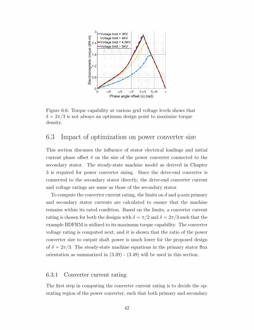
Figure 6.6: Torque capability at various grid voltage levels shows thatδ = 2π/3 is not always an optimum design point to maximize torquedensity.
6.3 Impact of optimization on power converter size
This section discusses the influence of stator electrical loadings and initial
current phase offset δ on the size of the power converter connected to the
secondary stator. The steady-state machine model as derived in Chapter
3 is required for power converter sizing. Since the drive-end converter is
connected to the secondary stator directly, the drive-end converter current
and voltage ratings are same as those of the secondary stator.
To compute the converter current rating, the limits on d and q-axis primary
and secondary stator currents are calculated to ensure that the machine
remains within its rated condition. Based on the limits, a converter current
rating is chosen for both the designs with δ = π/2 and δ = 2π/3 such that the
example BDFRM is utilized to its maximum torque capability. The converter
voltage rating is computed next, and it is shown that the ratio of the power
converter size to output shaft power is much lower for the proposed design
of δ = 2π/3. The steady-state machine equations in the primary stator flux
orientation as summarized in (3.39) - (3.49) will be used in this section.
6.3.1 Converter current rating
The first step in computing the converter current rating is to decide the op-
erating region of the power converter, such that both primary and secondary
42
stator currents remain within bounds, while yielding the demanded torque.
Neglecting the voltage drop across the primary stator resistance, the primary
stator flux is estimated as
ϕp =Vpwp
(6.11)
To remain within primary and secondary stator currents limits,
i2pd + i2pq ≤ I2prated (6.12)
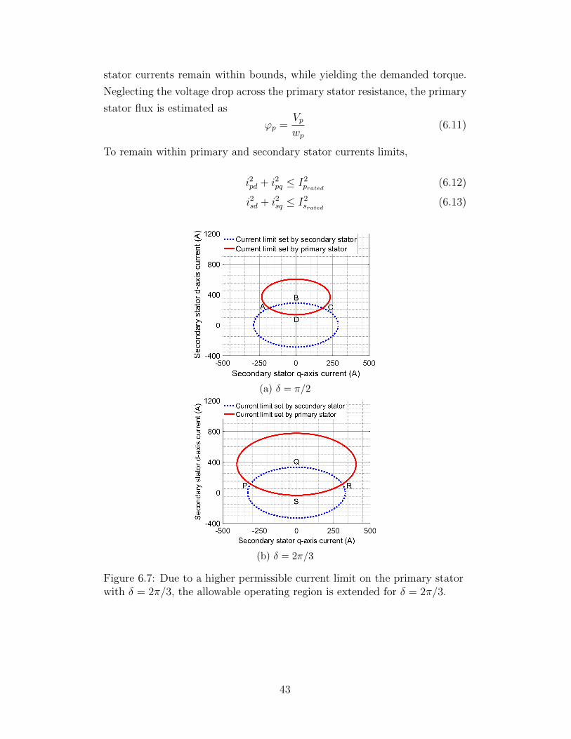
i2sd + i2sq ≤ I2srated (6.13)
(a) δ = π/2
(b) δ = 2π/3
Figure 6.7: Due to a higher permissible current limit on the primary statorwith δ = 2π/3, the allowable operating region is extended for δ = 2π/3.
43
The primary stator currents in (6.12) are substituted with the secondary
currents using (3.39) and (3.40):(ϕp − Lpsisd
Lp
)2
+
(LpsLp
isq
)2
≤ I2prated (6.14)
Both current constraints, given by Eqs. (6.13) and (6.14), are shown in Fig.
6.7. The overlapping region occupied by these curves, ABCD for δ = π/2,
as shown in Fig. 6.7(a), and PQRS for δ = 2π/3, as shown in Fig. 6.7(b),
is the area for safe operation. Phase offset δ = 2π/3 allows a much higher
primary stator current rating Iprated . This increase in current rating extends
both the major and minor axes of the ellipse given by (6.14) for δ = 2π/3,
extending the desired operating region as compared to δ = π/2.
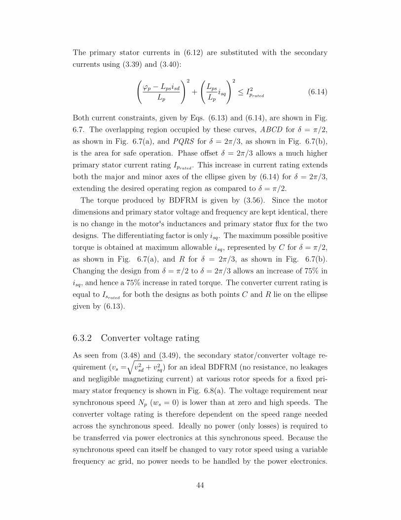
The torque produced by BDFRM is given by (3.56). Since the motor
dimensions and primary stator voltage and frequency are kept identical, there
is no change in the motor's inductances and primary stator flux for the two
designs. The differentiating factor is only isq. The maximum possible positive
torque is obtained at maximum allowable isq, represented by C for δ = π/2,
as shown in Fig. 6.7(a), and R for δ = 2π/3, as shown in Fig. 6.7(b).
Changing the design from δ = π/2 to δ = 2π/3 allows an increase of 75% in
isq, and hence a 75% increase in rated torque. The converter current rating is
equal to Israted for both the designs as both points C and R lie on the ellipse
given by (6.13).
6.3.2 Converter voltage rating
As seen from (3.48) and (3.49), the secondary stator/converter voltage re-
quirement (vs =√v2sd + v2sq) for an ideal BDFRM (no resistance, no leakages
and negligible magnetizing current) at various rotor speeds for a fixed pri-
mary stator frequency is shown in Fig. 6.8(a). The voltage requirement near
synchronous speed Np (ws = 0) is lower than at zero and high speeds. The
converter voltage rating is therefore dependent on the speed range needed
across the synchronous speed. Ideally no power (only losses) is required to
be transferred via power electronics at this synchronous speed. Because the
synchronous speed can itself be changed to vary rotor speed using a variable
frequency ac grid, no power needs to be handled by the power electronics.
44
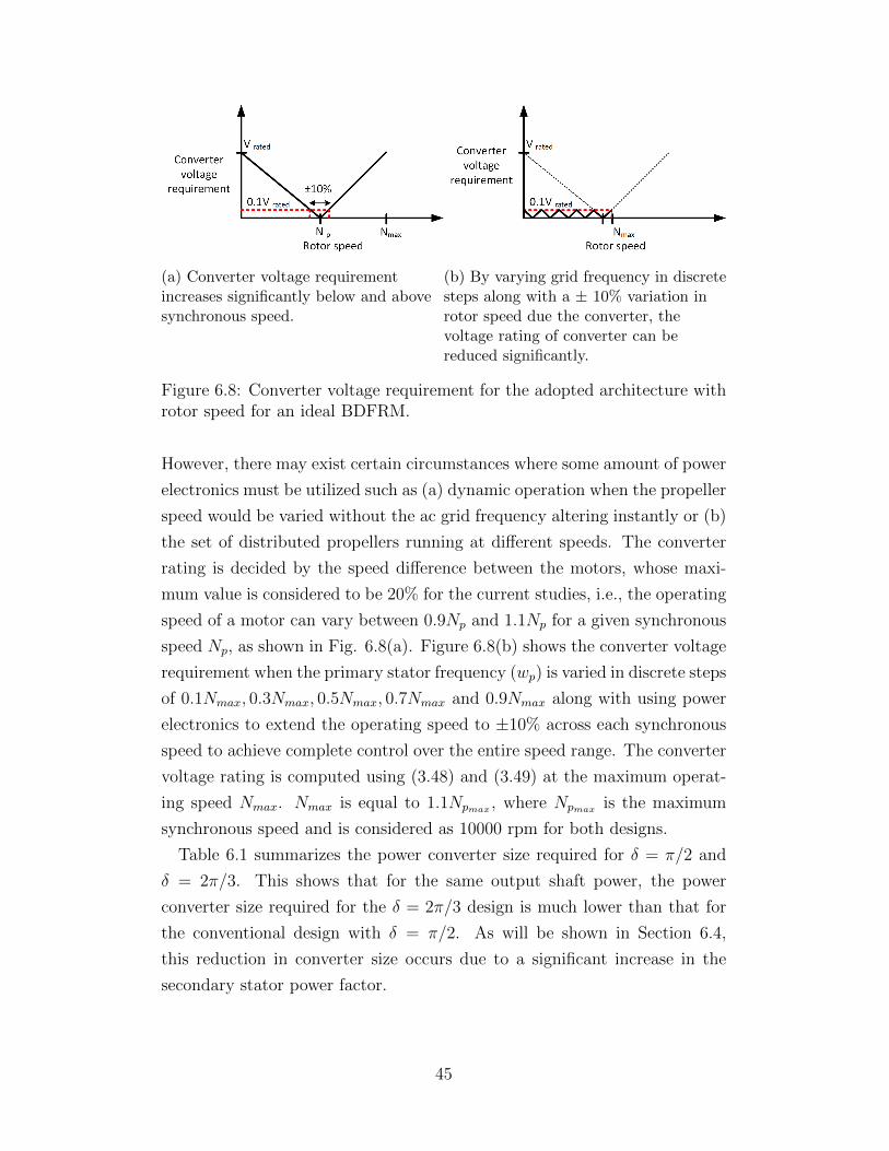
(a) Converter voltage requirementincreases significantly below and abovesynchronous speed.
(b) By varying grid frequency in discretesteps along with a ± 10% variation inrotor speed due the converter, thevoltage rating of converter can bereduced significantly.
Figure 6.8: Converter voltage requirement for the adopted architecture withrotor speed for an ideal BDFRM.
However, there may exist certain circumstances where some amount of power
electronics must be utilized such as (a) dynamic operation when the propeller
speed would be varied without the ac grid frequency altering instantly or (b)
the set of distributed propellers running at different speeds. The converter
rating is decided by the speed difference between the motors, whose maxi-
mum value is considered to be 20% for the current studies, i.e., the operating
speed of a motor can vary between 0.9Np and 1.1Np for a given synchronous
speed Np, as shown in Fig. 6.8(a). Figure 6.8(b) shows the converter voltage
requirement when the primary stator frequency (wp) is varied in discrete steps
of 0.1Nmax, 0.3Nmax, 0.5Nmax, 0.7Nmax and 0.9Nmax along with using power
electronics to extend the operating speed to ±10% across each synchronous
speed to achieve complete control over the entire speed range. The converter
voltage rating is computed using (3.48) and (3.49) at the maximum operat-
ing speed Nmax. Nmax is equal to 1.1Npmax , where Npmax is the maximum
synchronous speed and is considered as 10000 rpm for both designs.
Table 6.1 summarizes the power converter size required for δ = π/2 and
δ = 2π/3. This shows that for the same output shaft power, the power
converter size required for the δ = 2π/3 design is much lower than that for
the conventional design with δ = π/2. As will be shown in Section 6.4,
this reduction in converter size occurs due to a significant increase in the
secondary stator power factor.
45
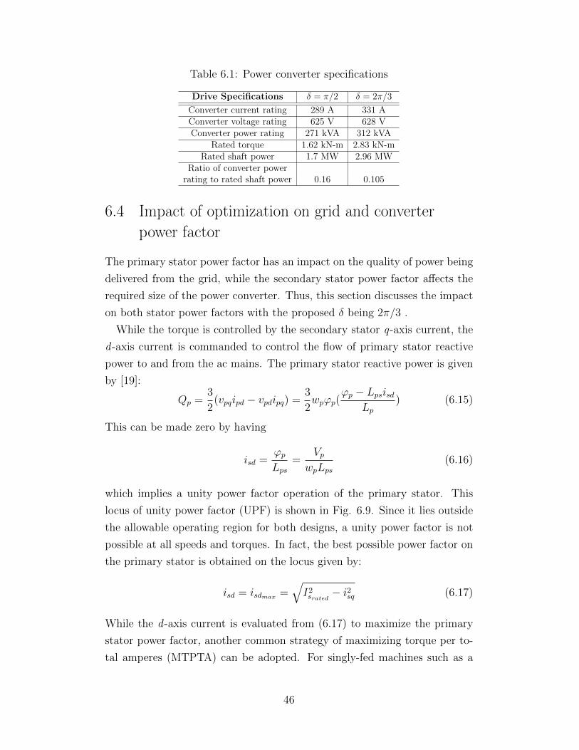
Table 6.1: Power converter specifications
Drive Specifications δ = π/2 δ = 2π/3
Converter current rating 289 A 331 AConverter voltage rating 625 V 628 VConverter power rating 271 kVA 312 kVA
Rated torque 1.62 kN-m 2.83 kN-mRated shaft power 1.7 MW 2.96 MW
Ratio of converter powerrating to rated shaft power 0.16 0.105
6.4 Impact of optimization on grid and converter
power factor
The primary stator power factor has an impact on the quality of power being
delivered from the grid, while the secondary stator power factor affects the
required size of the power converter. Thus, this section discusses the impact
on both stator power factors with the proposed δ being 2π/3 .
While the torque is controlled by the secondary stator q-axis current, the
d -axis current is commanded to control the flow of primary stator reactive
power to and from the ac mains. The primary stator reactive power is given
by [19]:
Qp =3
2(vpqipd − vpdipq) =
3
2wpϕp(
ϕp − LpsisdLp
) (6.15)
This can be made zero by having
isd =ϕpLps
=Vp
wpLps(6.16)
which implies a unity power factor operation of the primary stator. This
locus of unity power factor (UPF) is shown in Fig. 6.9. Since it lies outside
the allowable operating region for both designs, a unity power factor is not
possible at all speeds and torques. In fact, the best possible power factor on
the primary stator is obtained on the locus given by:
isd = isdmax =√I2srated − i2sq (6.17)
While the d -axis current is evaluated from (6.17) to maximize the primary
stator power factor, another common strategy of maximizing torque per to-
tal amperes (MTPTA) can be adopted. For singly-fed machines such as a
46
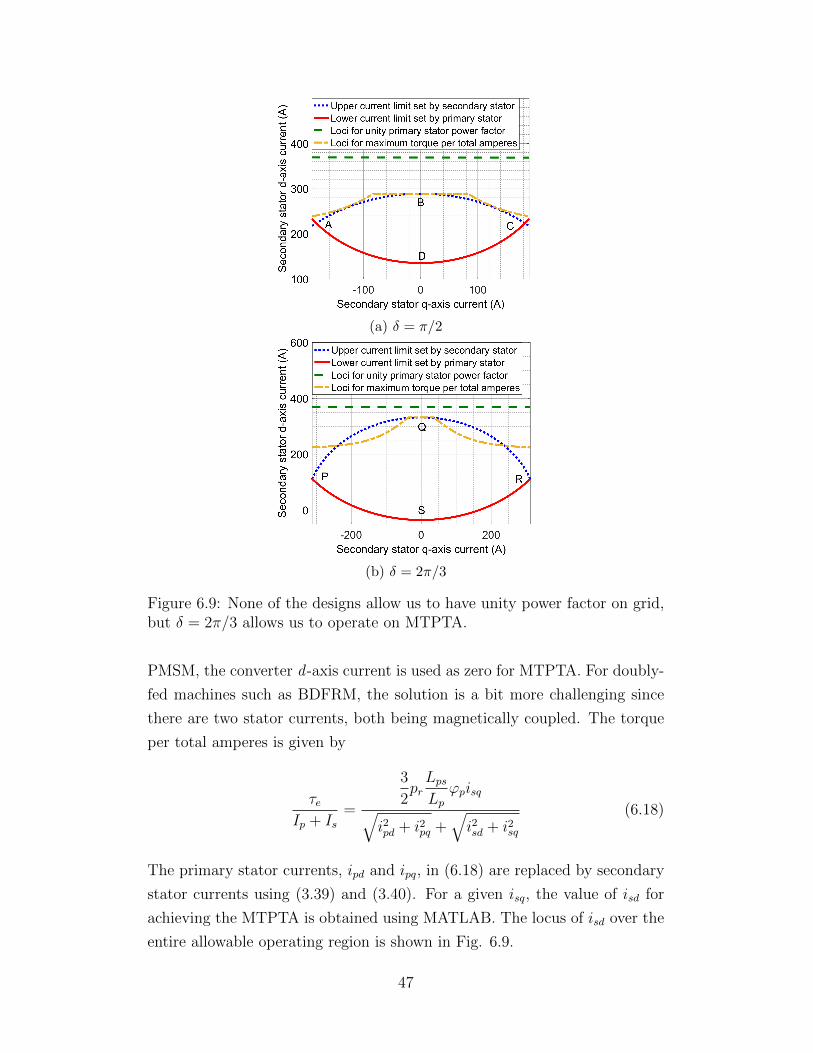
(a) δ = π/2
(b) δ = 2π/3
Figure 6.9: None of the designs allow us to have unity power factor on grid,but δ = 2π/3 allows us to operate on MTPTA.
PMSM, the converter d -axis current is used as zero for MTPTA. For doubly-
fed machines such as BDFRM, the solution is a bit more challenging since
there are two stator currents, both being magnetically coupled. The torque
per total amperes is given by
τeIp + Is
=
3
2prLpsLp
ϕpisq√i2pd + i2pq +
√i2sd + i2sq
(6.18)
The primary stator currents, ipd and ipq, in (6.18) are replaced by secondary
stator currents using (3.39) and (3.40). For a given isq, the value of isd for
achieving the MTPTA is obtained using MATLAB. The locus of isd over the
entire allowable operating region is shown in Fig. 6.9.
47
As seen from Fig. 6.4(b), there is a significant improvement of secondary
stator power factor at the rated conditions when δ changes from π/2 to 2π/3.
However this improvement is true at all operating points and not merely at
rated torque. The real and reactive power flowing into the secondary stator
are given by:
Ps =3
2(vsdisd + vsqiisq) (6.19)
Qs =3
2(vsqisd − vsdisq) (6.20)
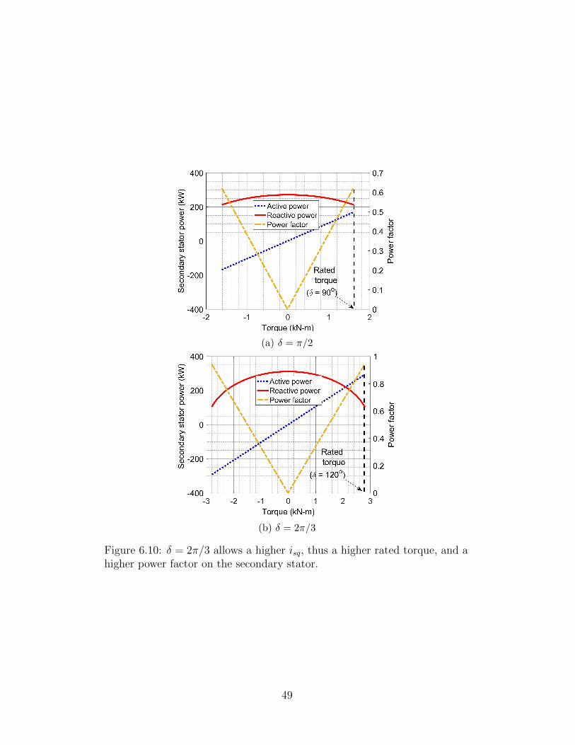
Both the real and reactive power flowing from the secondary stator at the
maximum operating speed wrmax are presented in Fig. 6.10 at various torque
conditions. This shows a significant improvement of power factor in the
secondary stator at all operating conditions when δ changes from π/2 to
2π/3. At rated torque, there is a considerable increase in the active power
being handled by the converter at δ = 2π/3 due to much higher rated torque.
Nevertheless, a significant improvement in the secondary stator power factor
decreases the reactive power handled by the converter at δ = 2π/3. The
power converter size remains almost constant for both the designs as seen
earlier in Section 6.3.
48
(a) δ = π/2
(b) δ = 2π/3
Figure 6.10: δ = 2π/3 allows a higher isq, thus a higher rated torque, and ahigher power factor on the secondary stator.
49
CHAPTER 7
FINITE ELEMENT ANALYSIS ANDRESULTS
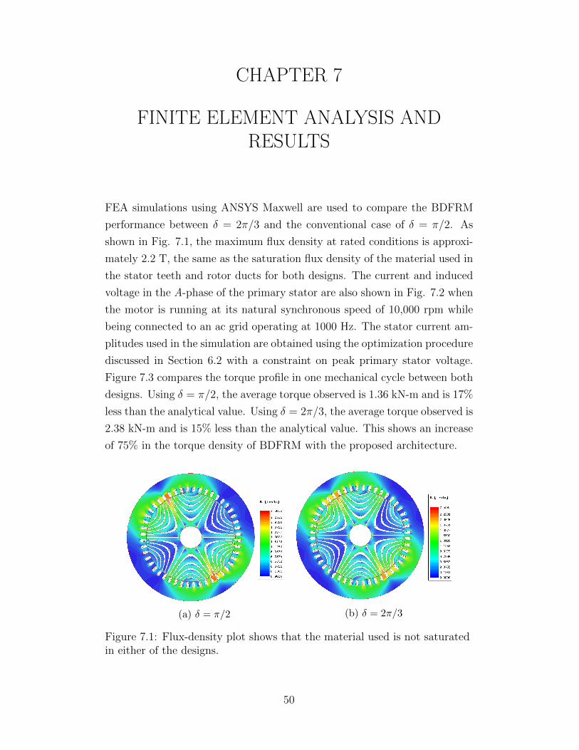
FEA simulations using ANSYS Maxwell are used to compare the BDFRM
performance between δ = 2π/3 and the conventional case of δ = π/2. As
shown in Fig. 7.1, the maximum flux density at rated conditions is approxi-
mately 2.2 T, the same as the saturation flux density of the material used in
the stator teeth and rotor ducts for both designs. The current and induced
voltage in the A-phase of the primary stator are also shown in Fig. 7.2 when
the motor is running at its natural synchronous speed of 10,000 rpm while
being connected to an ac grid operating at 1000 Hz. The stator current am-
plitudes used in the simulation are obtained using the optimization procedure
discussed in Section 6.2 with a constraint on peak primary stator voltage.
Figure 7.3 compares the torque profile in one mechanical cycle between both
designs. Using δ = π/2, the average torque observed is 1.36 kN-m and is 17%
less than the analytical value. Using δ = 2π/3, the average torque observed is
2.38 kN-m and is 15% less than the analytical value. This shows an increase
of 75% in the torque density of BDFRM with the proposed architecture.
(a) δ = π/2 (b) δ = 2π/3
Figure 7.1: Flux-density plot shows that the material used is not saturatedin either of the designs.
50
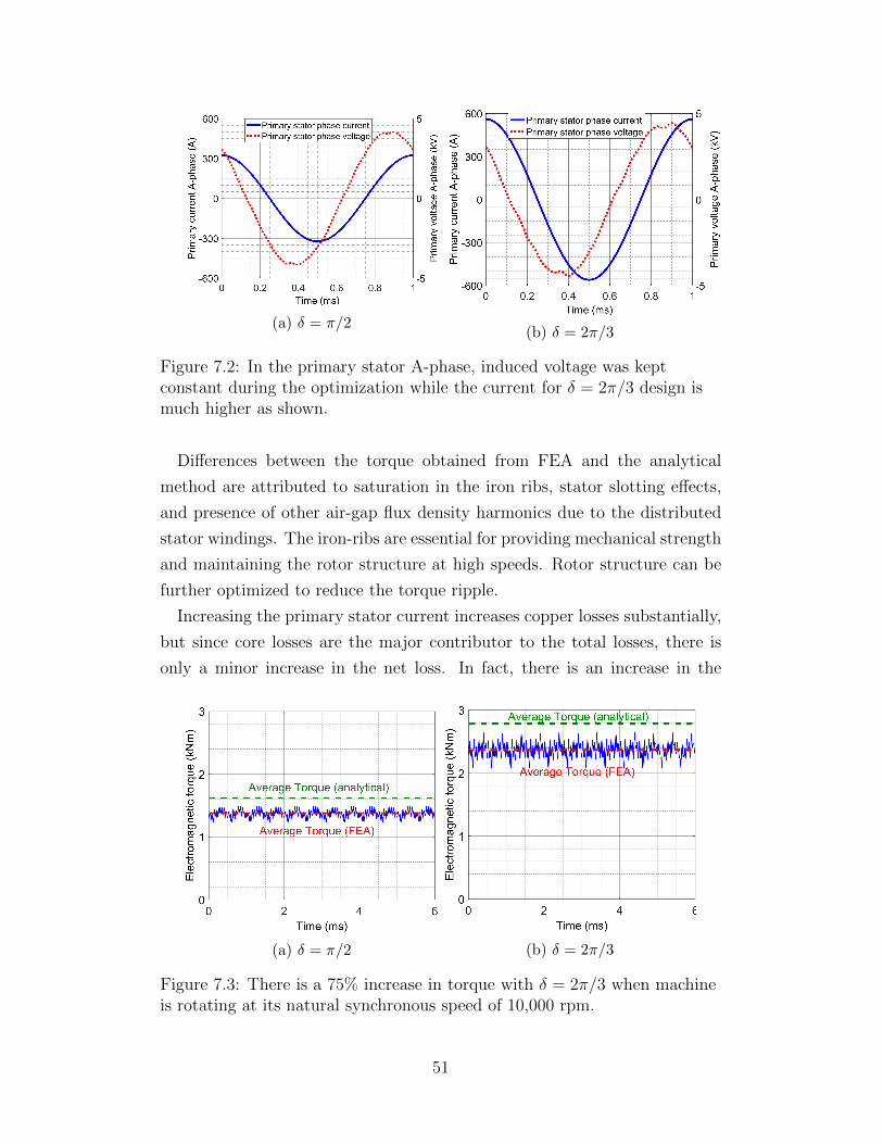
(a) δ = π/2(b) δ = 2π/3
Figure 7.2: In the primary stator A-phase, induced voltage was keptconstant during the optimization while the current for δ = 2π/3 design ismuch higher as shown.
Differences between the torque obtained from FEA and the analytical
method are attributed to saturation in the iron ribs, stator slotting effects,
and presence of other air-gap flux density harmonics due to the distributed
stator windings. The iron-ribs are essential for providing mechanical strength
and maintaining the rotor structure at high speeds. Rotor structure can be
further optimized to reduce the torque ripple.
Increasing the primary stator current increases copper losses substantially,
but since core losses are the major contributor to the total losses, there is
only a minor increase in the net loss. In fact, there is an increase in the
(a) δ = π/2 (b) δ = 2π/3
Figure 7.3: There is a 75% increase in torque with δ = 2π/3 when machineis rotating at its natural synchronous speed of 10,000 rpm.
51
Table 7.1: Performance comparison
Specifications δ = π/2 δ = 2π/3
Electrical loading (Ap, As) 10186 A/m, 9086 A/m 17605 A/m, 10469 A/mPower factor (cosθp, cosθs) 0.77, 0.63 0.8, 0.9
Torque 1.36 kN-m 2.38 kN-mCopper losses 1.14 kW 2.35 kW
Core losses 57 kW 70 kWEfficiency 96.1% 97.2%
overall efficiency with the proposed design. Table 7.1 shows the comparisons
between the two optimized designs with δ = π/2 and δ = 2π/3.
A 1.5 MW BDFRM for a rated speed of 10,000 rpm is designed with
δ = 2π/3 and optimum stator currents using (6.8). An air gap of 2 mm
was selected as a feasible value considering cooling requirements. The motor
dimensions and weight are listed in Table 7.2. Active material weight is
obtained from FEA software, where all the inactive material including shaft,
insulation material, and motor housing are neglected for this study. A rib-
width of 3 mm is selected to provide adequate mechanical integrity after
conducting the rotor stress analysis.
The motor current and voltage ratings, and its performance at rated con-
ditions, are listed in Table 7.3. Since the motor is running at such a high
speed, it is necessary to include windage loss in the efficiency computation.
The windage loss is predicted using the model in [35]. Figure 7.4 shows the
2-D cross sectional area of the designed 1.5 MW motor. Figure 7.5 shows
the torque profile for one mechanical rotation cycle. The torque ripple is
approximately 17%.
Table 7.2: BDFRM dimensions
Parameter Value
Air-gap diameter 420 mmStator outer diameter 575 mm
Stack length 400 mmShaft diameter 120 mm
Air-gap 2 mmNumber of stator slots 48Number of rotor ducts 66
Slot depth 25 mmActive weight 671 kg
52
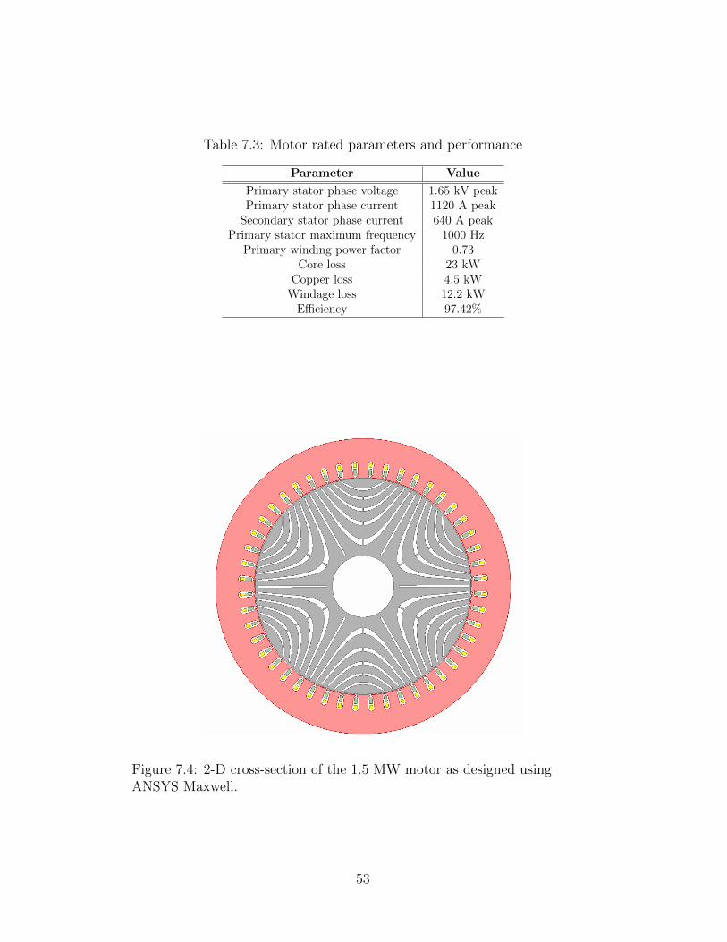
Table 7.3: Motor rated parameters and performance
Parameter Value
Primary stator phase voltage 1.65 kV peakPrimary stator phase current 1120 A peak
Secondary stator phase current 640 A peakPrimary stator maximum frequency 1000 Hz
Primary winding power factor 0.73Core loss 23 kW
Copper loss 4.5 kWWindage loss 12.2 kW
Efficiency 97.42%
Figure 7.4: 2-D cross-section of the 1.5 MW motor as designed usingANSYS Maxwell.
53
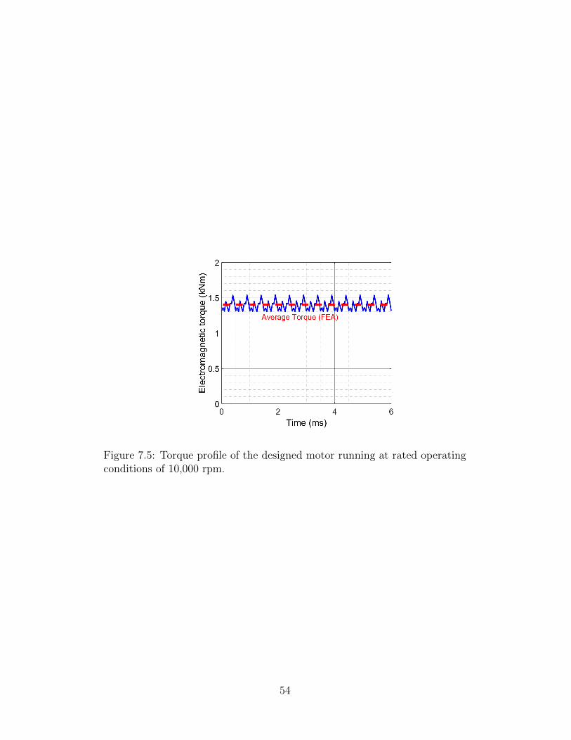
Figure 7.5: Torque profile of the designed motor running at rated operatingconditions of 10,000 rpm.
54
CHAPTER 8
CONCLUSIONS
8.1 Summary and design insights
This thesis has addressed a wide range of topics within the scope of electric
machine development for turbo-electric aircraft propulsion systems. With the
ever increasing demand for air travel, it is essential to explore more energy-
efficient means for deployment in the commercial aviation industry. This
motivates the use of electric machines to drive the propeller fans, hence de-
coupling the speed of turbine and propeller. Brushless doubly-fed reluctance
machines (BDFRM) are seen as an attractive choice to drive the distributed
propeller fans as they use partially rated power converter, have brushless op-
eration, and low rotor losses. This thesis explores a BDFRM by computing
the machine and power converter size for the rated operation.
The motor developed after the initial sizing, and following the conventional
approach of having equal electrical loadings on both the stator windings, has
poor torque density. This thesis presents an approach to enhance torque
density. A single objective function along with multiple constraints is formu-
lated in terms of three design variables: electrical loadings of primary and
secondary stators, and phase offset in the secondary stator current (δ), which
plays a role similar to the torque angle in a synchronous motor. Optimization
results reveal that the most commonly used δ = π/2 is not an optimum op-
erating point in terms of torque. Phase offset δ = 2π/3, along with suitable
electrical loadings, has the capability to increase the torque by 75%. There is
also an improvement in efficiency and power factor. 2-D FEA using ANSYS
Maxwell was also carried out to validate the optimization results.
55
8.2 Future work
The following future work will be done during the author's PhD program:
� The rotor is modeled having infinite number of ducts for ease of analyt-
ical formulation. The rotor will be modeled considering finite widths of
iron ducts and air-barriers using reluctance network. This can enhance
the rotor modeling, leading to a more accurate prediction of torque
density improvement.
� The copper and core losses are computed using FEA. A framework
for the loss computation will be developed. Considering the amount
of flux-density harmonics in the material in this type of machine, the
modeling of core loss will be challenging but needs to be looked at for
maximizing efficiency.
� A switched drive architecture similar to the one presented in [36] will be
investigated. A motor in an electrical aircraft operates under various
operating conditions. The maximum torque or the rated conditions are
required during take-off, which lasts only a few minutes. The motor
needs to be operated at a significantly lower torque and speed at cruise.
Since the cruise conditions last for several hours, these conditions de-
mand the motor to be efficient at operating points far away from rated
ones. Designing the motor to operate efficiently at low speeds while
delivering the required torque at high speeds is the key for such appli-
cations and can probably be achieved using switched drive architecture.
� Since the motor is running at speeds close to 10,000 rpm, the mechan-
ical integrity of the rotor needs to be investigated. A trade-off study
between the output torque and the stress for different rotor iron rib
widths will be done to ensure the motor is capable of delivering suffi-
cient torque while maintaining mechanical integrity.
� A 5-hp prototype motor will be designed, constructed, tested and val-
idated along with developing necessary drive control algorithms.
56
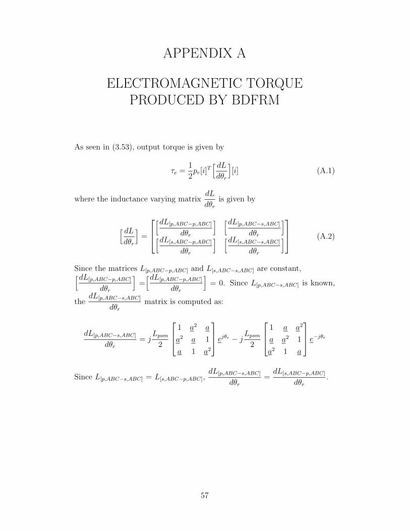
APPENDIX A
ELECTROMAGNETIC TORQUEPRODUCED BY BDFRM
As seen in (3.53), output torque is given by
τe =1
2pr[i]
T[ dLdθr
][i] (A.1)
where the inductance varying matrixdL
dθris given by
[ dLdθr
]=
[dL[p,ABC−p,ABC]
dθr
] [dL[p,ABC−s,ABC]
dθr
][dL[s,ABC−p,ABC]
dθr
] [dL[s,ABC−s,ABC]
dθr
] (A.2)
Since the matrices L[p,ABC−p,ABC] and L[s,ABC−s,ABC] are constant,[dL[p,ABC−p,ABC]
dθr
]=[dL[p,ABC−p,ABC]
dθr
]= 0. Since L[p,ABC−s,ABC] is known,
thedL[p,ABC−s,ABC]
dθrmatrix is computed as:
dL[p,ABC−s,ABC]
dθr= j
Lpsm2
1 a2 a
a2 a 1
a 1 a2
ejθr − jLpsm2
1 a a2
a a2 1
a2 1 a
e−jθr
Since L[p,ABC−s,ABC] = L[s,ABC−p,ABC],dL[p,ABC−s,ABC]
dθr=dL[s,ABC−p,ABC]
dθr.
57
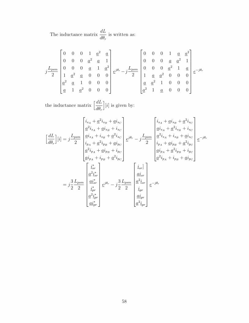
The inductance matrixdL
dθris written as:
jLpsm
2
0 0 0 1 a2 a
0 0 0 a2 a 1
0 0 0 a 1 a2
1 a2 a 0 0 0
a2 a 1 0 0 0
a 1 a2 0 0 0
ejθr−jLpsm
2
0 0 0 1 a a2
0 0 0 a a2 1
0 0 0 a2 1 a
1 a a2 0 0 0
a a2 1 0 0 0
a2 1 a 0 0 0
e−jθr
the inductance matrix[ dLdθr
][i] is given by:
[ dLdθr
][i] = j
Lpsm2
isA + a2isB + aisCa2isA + aisB + isCaisA + isB + a2isCipA + a2ipB + aipCa2ipA + aipB + ipCaipA + ipB + a2ipC
ejθr − jLpsm
2
isA + aisB + a2isCaisA + a2isB + isCa2isA + isB + aisCipA + aipB + a2ipCaipA + a2ipB + ipCa2ipA + ipB + aipC
e−jθr
= j3
2
Lpsm2
i∗sr
a2i∗sr
ai∗sr
i∗pr
a2i∗pr
ai∗pr
ejθr − j 3
2
Lpsm2
isr]
aisr
a2isr
ipr
aipr
a2ipr
e−jθr
58
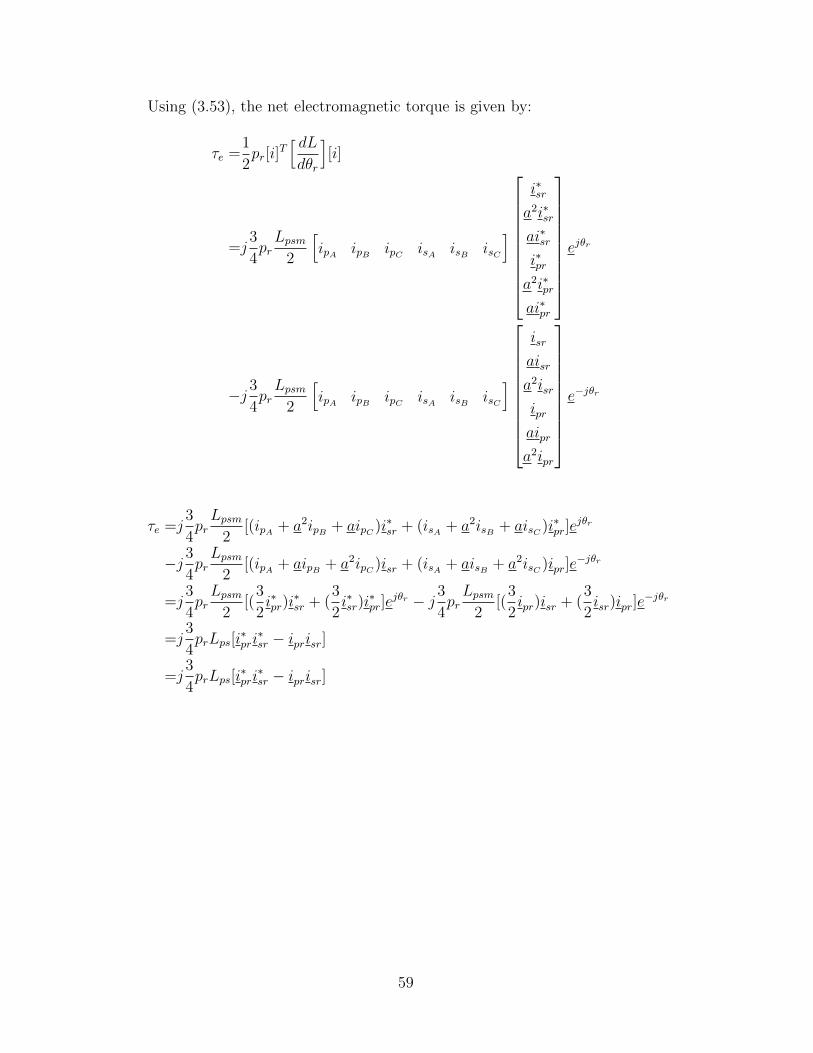
Using (3.53), the net electromagnetic torque is given by:
τe =1
2pr[i]
T[ dLdθr
][i]
=j3
4prLpsm
2
[ipA ipB ipC isA isB isC
]
i∗sr
a2i∗sr
ai∗sr
i∗pr
a2i∗pr
ai∗pr
ejθr
−j 3
4prLpsm
2
[ipA ipB ipC isA isB isC
]
isr
aisr
a2isr
ipr
aipr
a2ipr
e−jθr
τe =j3
4prLpsm
2[(ipA + a2ipB + aipC )i∗sr + (isA + a2isB + aisC )i∗pr]e
jθr
−j 3
4prLpsm
2[(ipA + aipB + a2ipC )isr + (isA + aisB + a2isC )ipr]e
−jθr
=j3
4prLpsm
2[(
3
2i∗pr)i
∗sr + (
3
2i∗sr)i
∗pr]e
jθr − j 3
4prLpsm
2[(
3
2ipr)isr + (
3
2isr)ipr]e
−jθr
=j3
4prLps[i
∗pri∗sr − iprisr]
=j3
4prLps[i
∗pri∗sr − iprisr]
59
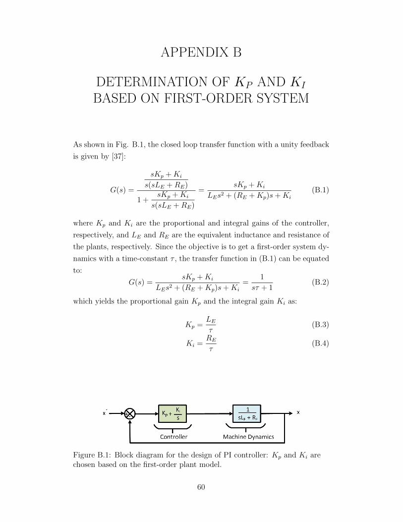
APPENDIX B
DETERMINATION OF KP AND KI
BASED ON FIRST-ORDER SYSTEM
As shown in Fig. B.1, the closed loop transfer function with a unity feedback
is given by [37]:
G(s) =
sKp +Ki
s(sLE +RE)
1 +sKp +Ki
s(sLE +RE)
=sKp +Ki
LEs2 + (RE +Kp)s+Ki
(B.1)
where Kp and Ki are the proportional and integral gains of the controller,
respectively, and LE and RE are the equivalent inductance and resistance of
the plants, respectively. Since the objective is to get a first-order system dy-
namics with a time-constant τ , the transfer function in (B.1) can be equated
to:
G(s) =sKp +Ki
LEs2 + (RE +Kp)s+Ki
=1
sτ + 1(B.2)
which yields the proportional gain Kp and the integral gain Ki as:
Kp =LEτ
(B.3)
Ki =RE
τ(B.4)
Figure B.1: Block diagram for the design of PI controller: Kp and Ki arechosen based on the first-order plant model.
60
REFERENCES
[1] T. Houser, H. Pitt, and H. Hess, “Final US emissions estimates for2019,” prepared by the Rhodium Group for the US Climate Service,2019.
[2] National Academies of Science, Engineering, and Medicine, Commer-cial Aircraft Propulsion and Energy Systems Research: Reducing GlobalCarbon Emissions. National Academies Press, 2016.
[3] R. Jansen, C. Bowman, A. Jankovsky, R. Dyson, and J. Felder,“Overview of NASA electrified aircraft propulsion (EAP) research forlarge subsonic transports,” in 53rd AIAA/SAE/ASEE Joint PropulsionConference, 2017, p. 4701.
[4] P. Gemin, T. Kupiszewski, A. Radun, Y. Pan, R. Lai, D. Zhang,R. Wang, X. Wu, Y. Jiang, S. Galioto et al., “Architecture, voltage,and components for a turboelectric distributed propulsion electric grid(AVC-TeDP),” NASA/CR-2015-218713, 2015.
[5] A. D. Anderson, N. J. Renner, Y. Wang, S. Agrawal, S. Sirimanna,D. Lee, A. Banerjee, K. Haran, M. J. Starr, and J. L. Felder, “Systemweight comparison of electric machine topologies for electric aircraftpropulsion,” in 2018 AIAA/IEEE Electric Aircraft Technologies Sym-posium (EATS). IEEE, 2018, pp. 1–16.
[6] M. J. Armstrong, M. Blackwelder, A. Bollman, C. Ross, A. Campbell,C. Jones, and P. Norman, “Architecture, voltage, and components fora turboelectric distributed propulsion electric grid,” NASA/CR-2015-218440, 2015.
[7] D. J. Sadey, M. Bodson, J. Csank, K. Hunker, C. Theman, and L. Tay-lor, “Control demonstration of multiple doubly-fed induction motors forhybrid electric propulsion,” in 53rd AIAA/SAE/ASEE Joint PropulsionConference, 2017, p. 4954.
[8] S. Agrawal, A. Banerjee, and R. F. Beach, “Brushless doubly-fed reluc-tance machine drive for turbo-electric distributed propulsion systems,”in 2018 AIAA/IEEE Electric Aircraft Technologies Symposium (EATS).IEEE, 2018, pp. 1–17.
61
[9] L. Xu, B. Guan, H. Liu, L. Gao, and K. Tsai, “Design and control of ahigh-efficiency doubly-fed brushless machine for wind power generatorapplication,” in 2010 IEEE Energy Conversion Congress and Exposition.IEEE, 2010, pp. 2409–2416.
[10] M.-F. Hsieh, Y.-H. Chang, and D. G. Dorrell, “Design and analysis ofbrushless doubly fed reluctance machine for renewable energy applica-tions,” IEEE Transactions on Magnetics, vol. 52, no. 7, pp. 1–5, 2016.
[11] D. Gay, R. Betz, D. Dorrell, and A. Knight, “Grid fault performance ofbrushless doubly-fed reluctance machines in wind turbine applications,”in 2018 20th European Conference on Power Electronics and Applica-tions (EPE’18 ECCE Europe). IEEE, 2018, pp. P–1.
[12] S. Agrawal and A. Banerjee, “Switched brushless doubly-fed reluctancemachine drive for wide-speed range applications,” in 2018 IEEE EnergyConversion Congress and Exposition (ECCE). IEEE, 2018, pp. 4473–4480.
[13] A. M. Knight, R. E. Betz, and D. G. Dorrell, “Design and analysisof brushless doubly fed reluctance machines,” IEEE Transactions onIndustry Applications, vol. 49, no. 1, pp. 50–58, 2012.
[14] S. Agrawal, A. Province, and A. Banerjee, “An approach to maximizetorque density in a brushless doubly-fed reluctance machine,” in 2019IEEE Energy Conversion Congress and Exposition (ECCE). IEEE, pp.298–305.
[15] M. Cheng, P. Han, and W. Hua, “General airgap field modulation theoryfor electrical machines,” IEEE Transactions on Industrial Electronics,vol. 64, no. 8, pp. 6063–6074, 2017.
[16] T. Staudt, F. Wurtz, N. J. Batistela, and P. Kuo-Peng, “Influence of ro-tor design and geometric parameter variation on global performance ofbrushless doubly-fed reluctance machines,” in 2014 International Con-ference on Electrical Machines (ICEM). IEEE, 2014, pp. 537–543.
[17] I. Boldea, Z. Fu, and S. Nasar, “Performance evaluation of axially-laminated anisotropic (ALA) rotor reluctance synchronous motors,”IEEE transactions on industry applications, vol. 30, no. 4, pp. 977–985,1994.
[18] A. Vagati, M. Pastorelli, G. Francheschini, and S. C. Petrache, “De-sign of low-torque-ripple synchronous reluctance motors,” IEEE Trans-actions on Industry Applications, vol. 34, no. 4, pp. 758–765, 1998.
62
[19] R. E. BETZ and M. Jovanovic, “Introduction to the space vector mod-eling of the brushless doubly fed reluctance machine,” Electric PowerComponents and Systems, vol. 31, no. 8, pp. 729–755, 2003.
[20] E. Schulz and R. Betz, “Optimal torque per amp for brushless dou-bly fed reluctance machines,” in Fortieth IAS Annual Meeting. Confer-ence Record of the 2005 Industry Applications Conference, 2005, vol. 3.IEEE, 2005, pp. 1749–1753.
[21] S. Agrawal and A. Banerjee, “Torque-density improvement in brush-less doubly-fed reluctance machines using additional stator winding,”in 2019 IEEE International Electric Machines & Drives Conference(IEMDC). IEEE, 2019, pp. 314–321.
[22] R. Betz and M. Jovanovic, “Introduction to brushless doubly fed re-luctance machines-the basic equations,” Dept. Elec. Energy Conversion,Aalborg University, 1998.
[23] M. G. Jovanovic, R. E. Betz, and J. Yu, “The use of doubly fed reluc-tance machines for large pumps and wind turbines,” IEEE Transactionson Industry Applications, vol. 38, no. 6, pp. 1508–1516, 2002.
[24] M. Jovanovic, “Sensored and sensorless speed control methods for brush-less doubly fed reluctance motors,” IET Electric Power Applications,vol. 3, no. 6, pp. 503–513, 2009.
[25] L. Xu, L. Zhen, and E.-H. Kim, “Field orientation control of a doublyexcited brushless reluctance machine,” in IAS’96. Conference Recordof the 1996 IEEE Industry Applications Conference Thirty-First IASAnnual Meeting, vol. 1. IEEE, 1996, pp. 319–325.
[26] S. Ademi and M. G. Jovanovic, “Vector control methods for brushlessdoubly fed reluctance machines,” IEEE Transactions on Industrial Elec-tronics, vol. 62, no. 1, pp. 96–104, 2014.
[27] M. Jovanovic, J. Yu, and E. Levi, “Direct torque control of brushlessdoubly fed reluctance machines,” Electric Power Components and Sys-tems, vol. 32, no. 10, pp. 941–958, 2004.
[28] N. R. N. Idris and A. H. M. Yatim, “An improved stator flux esti-mation in steady-state operation for direct torque control of inductionmachines,” IEEE Transactions on Industry Applications, vol. 38, no. 1,pp. 110–116, 2002.
[29] T. Staudt, “Brushless doubly-fed reluctance machine modeling, designand optimization,” Ph.D. dissertation, The Federal University of SantaCatarina, 2015.
63
[30] W. Soong, “Sizing of electrical machines,” Power Engineering BriefingNote Series, vol. 9, pp. 17–18, 2008.
[31] A. Yoon, X. Yi, J. Martin, Y. Chen, and K. Haran, “A high-speed, high-frequency, air-core pm machine for aircraft application,” in 2016 IEEEPower and Energy Conference at Illinois (PECI). IEEE, 2016, pp. 1–4.
[32] X. Wang, R. McMahon, and P. Tavner, “Design of the brushless doubly-fed (induction) machine,” in 2007 IEEE International Electric Machines& Drives Conference, vol. 2. IEEE, 2007, pp. 1508–1513.
[33] T. A. Lipo, Introduction to AC Machine Design. John Wiley & Sons,2017, vol. 63.
[34] X. Zhang, C. L. Bowman, T. C. O’Connell, and K. S. Haran, “Largeelectric machines for aircraft electric propulsion,” IET Electric PowerApplications, vol. 12, no. 6, pp. 767–779, 2018.
[35] J. E. Vrancik, “Prediction of windage power loss in alternators,” NASATN D-4849, 1968.
[36] A. Banerjee et al., “Switched-doubly-fed-machine drive for high powerapplications,” Ph.D. dissertation, Massachusetts Institute of Technol-ogy, 2016.
[37] N. S. Nise, Control Systems Engineering, John Wiley & Sons, 2007.
64


![Design of Experiments (DoE) & Development of Design Space (DS) by Shivang Chaudhary [MS Pharma (Pharmaceutics)]](https://img.pdfslide.us/doc/110x75/5470666daf7959a41e8b474b/design-of-experiments-doe-development-of-design-space-ds-by-shivang-chaudhary-ms-pharma-pharmaceutics.jpg)