2017-2018 – Econ 3029 – Advanced Macro

Lecture 3 : Income and Wealth Inequalities

Franck PortierF.Portier@UCL.ac.uk

University College London

Version 1.127/02/2018

Changes from version 1.0 are in red

1 / 51

Disclaimer

These are the slides I am using in class. They are not self-contained, do not alwaysconstitute original material and do contain some “cut and paste” pieces from varioussources that might not always explicitly referring to (although I am trying to cite mysources as much as possible). Therefore, they are not intended to be used outside ofthe course nor to be distributed. Thank you for signalling me typos or mistakes atF.Portier@UCL.ac.uk.

2 / 51

0. IntroductionWhat is this lecture about ?

I Recent extraordinary success of Thomas Piketty’sbook Capital in the Twenty-First Century

I Main questions

× How did inequalities evolved over the last century ?(income, wealth, capital income)

× What can we expect for the future ?× r > g ?

I According to Ricardo in the preface of his Principles ofPolitical Economy and Taxation (1817), thedetermination of the laws of distribution is :“the principal problem in Political Economy.”

Figure 1 – Piketty’sbook cover

3 / 51

0. IntroductionPlan of the Lecture

1. Income distribution in history of economic thought

2. Kuznets’ Facts

3. Piketty’s Facts

4. Piketty’s two ”laws of capitalism”

5. ky in the Solow model and beyond

6. The elasticity of substitution between k and `

7. Summary

8. References

4 / 51

1. Income distribution in history of economic thoughtIncome distribution

I Two distinct concepts

× Functional distribution of income, i.e. the distribution of income between the mainfactors of production : capital, labor, land

× Personal distribution of income between individuals : wage inequalities, capital orland ownership

I Two different level of analysis

× Positive : Why are some people rich and some poor ?× Normative : Which level of inequalities is justified ?

I I am discussing only the positive aspect and mainly functional distribution.

5 / 51

1. Income distribution in history of economic thoughtAdam Smith (1723-1790)

I 1776 : An Inquiry into the Nature and Causes of theWealth of Nations

I Division of labor makes it possible to increase laborproductivity

× Pin factory× The production of a pin has been broken down into

“about eighteen” separate operations,× Productivity is multipied by 4800.

I but no proportional increase in the wage... why ?

I Main reason : any increase in the general level of wageswould lead to an increase of population and therefore ofthe work force, and this would tend to reverse the initialincrease of wages.

I Typical effect in the “malthusian regime”

Figure 2 – Adam Smith

6 / 51

1. Income distribution in history of economic thoughtDavid Ricardo (1772-1823)

I 1817 : Principles of Political Economy and Taxation

I Wages are explained by the Malthusian dynamics alreadydescribed by Adam Smith

I Profits (capital income) is the rate of return on capital,defined as the rate of interest plus a risk premium.

I The other really important factor (besides labor) is land.

I Rent is the income that goes to land owners.

Figure 3 – David Ricardo

7 / 51

1. Income distribution in history of economic thoughtDavid Ricardo on rent

I Scarcity principle

I Land varies in terms of its quality or productivity.

I Ricardo’s generic term for agricultural products : corn

I The price of corn is determined by the cost of labour and capital required toproduce a unit of corn on the land with the lowest quality.

I Corn has same quality on all types of land all corn will sell at the same price

I Therefore, a positive rent will exist on all inframarginal units of land.

8 / 51

1. Income distribution in history of economic thoughtDavid Ricardo on rent (continued)

I Rent is determined by the cost of labour and capital used on the margin ofcultivation,

I and the position of this margin is determined by the price of corn.

I “Corn [price] is not high because a rent is paid, but a rent is paid because corn[price] is high”, Ricardo (1817)

I What is the dynamics of a growing economy (for example with technologicalprogress) ?

× wages increase above the level of subsistence population expands demand forcorn increases the margin of cultivation is extended.

× The share of rent and wages in national income go up× even after the wage rate has returned to its level of subsistence (because population

is larger).× The implication of this is that profits fall× weakening of the incentive to invest the economy reaches its stationary state,

9 / 51

1. Income distribution in history of economic thoughtDavid Ricardo’s principle of scarcity

I Land tends to become increasingly scarce relative to other goods.

I Land owners will therefore claim a growing share of national income, as the shareavailable to the rest of the population decreases

I Risks of social and political instability.

I For Ricardo, the only logically and politically acceptable answer was to impose asteadily increasing tax on land rents.

I The Ricardian principle of scarcity is still important to understand the distributionof wealth in the twenty-first century.

I Replace the price of farmland in Ricardo’s model by

× the price of urban real estate in major world capitals× the price of oil.

10 / 51

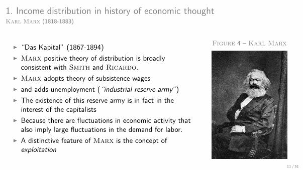
1. Income distribution in history of economic thoughtKarl Marx (1818-1883)

I “Das Kapital” (1867-1894)

I Marx positive theory of distribution is broadlyconsistent with Smith and Ricardo.

I Marx adopts theory of subsistence wages

I and adds unemployment (“industrial reserve army”)

I The existence of this reserve army is in fact in theinterest of the capitalists

I Because there are fluctuations in economic activity thatalso imply large fluctuations in the demand for labor.

I A distinctive feature of Marx is the concept ofexploitation

Figure 4 – Karl Marx

11 / 51

1. Income distribution in history of economic thoughtKarl Marx’s concept of exploitation

I Labour is the fundamental factor of production in the sense that all non-labourinputs can be derived from past labour.

I “all commodities are only definite masses of congealed labour time”, “DasKapital”, 1867-1894

I But workers are only paid the subsistence wage

I The difference between the two is the worker’s unpaid work for the benefit of thecapitalist.

I This is the profit or surplus value which defines the capitalist’s exploitation of theworker.

12 / 51

1. Income distribution in history of economic thoughtDynamics of capitalist economies for Marx

I Capital is primarily industrial (machinery, plants, etc.) rather than landed property,

I In principle there is no limit to the amount of capital that could be accumulated.

I inexorable tendency for capital to accumulate and become concentrated in everfewer hands.

I two alternative ends :

× the rate of return on capital steadily diminishes kills the engine of accumulationand leads to violent conflict among capitalists,

× capital’s share of national income increases indefinitely social revolts

13 / 51

1. Income distribution in history of economic thoughtThe marginalist approach

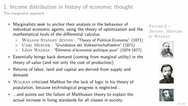
I Marginalists seek to anchor their analysis in the behaviour ofindividual economic agents, using the theory of optimization and themathematical tools of the differential calculus.

× William Stanley Jevons : “Theory of Political Economy” (1871)× Carl Menger : “Grundsatze der Volkswirtschaftslehre” (1871)× Leon Walras : “Elements d’economie politique pure” (1874-1877).

I Essentially brings back demand (coming from marginal utility) in thetheory of value (and not only the cost of production)

I Returns of labor, land and capital are derived from supply anddemand

I Walras criticized Malthus for the lack of logic in his theory ofpopulation, because technological progress is neglected...

I ...and points out the failure of Malthusian theory to explain theactual increase in living standards for all classes in society.

Figure 5 –Jevons, Menger& Walras

14 / 51

1. Income distribution in history of economic thoughtModern Neoclassical Theory

I Consider the Solow model as illustrative of the modern theory.

I Constant saving rate + Neoclassical production function

I Exogenous technical progress

I Existence of a Balance Growth Path along which the shares of capital and laborare constant.

I Sustained growth without (functional) inequalities explosion.

15 / 51

1. Income distribution in history of economic thoughtDynamics

I Classics and Marx : Stationary state with subsistance wage or collapse

I Neoclassical economics : Balanced growth is possible (Solow)

I All this theory has been developed with virtually no data ... until Kuznets in the1950’s.

16 / 51

2. Kuznets’ FactsMethod

I Simon Kuznets : American economist (Russian immigrant, 1901-1985)

I 1953 book : “Shares of Upper Income Groups in Income and Savings”

I United States from 1913 to 1948I First publication that uses two sources of data

× US federal income tax returns (which did not exist before the creation of the incometax in 1913)

× US national accounts

I Kuznets can compute the evolution of the share of each decile, as well as of theupper centiles, of the income hierarchy in total US national income.

17 / 51

2. Kuznets’ FactsFindings

I Sharp reduction in income inequality in the United States between 1913 and 1948

I The upper decile of the income distribution went down from 45-50 % of annualnational income to 30-35 %

I This 10% of income reduction is equal to half of the income of the poorest 50percent of Americans

I Bottom line : Inequalities are reducing

18 / 51

2. Kuznets’ FactsKuznets curve

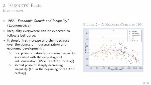
I 1955 “Economic Growth and Inequality”(Econometrica)

I Inequality everywhere can be expected tofollow a bell curve.

I It should first increase and then decreaseover the course of industrialization andeconomic development :

× first phase of naturally increasing inequalityassociated with the early stages ofindustrialization (US in the XIXth century)

× second phase of sharply decreasinginequality (US in the beginning of the XXthcentury)

Figure 6 – A Kuznets Curve in 1990Figure 3: Inequality in a Cross Section of Countries with a Quadratic Fit

2030

4050

6070

Gin

i ceo

ffici

ent

250 500 1000 2000 4000 8000 16000 32000 64000GDP per capita (PPP)

OECD902

Latin AmericaE. Europe & FSUAfricaAsiaQuadratic fit

Figure 4: Quadratic Fit of Inequality in a Cross Section of Countries without a Logarithmic Scale

2030

4050

6070

Gin

i ceo

ffici

ent

0 10000 20000 30000 40000 50000GDP per capita (PPP)

OECD902

Latin AmericaE. Europe & FSUAfricaAsiaQuadratic fit

19 / 51

3. Piketty’s factsCapital in the Twenty-First Century

I Thomas Piketty book published in 2014

I He puts together data on income and wealth inequalities for many countries overa long period

I Here I consider U.S. and Europe

I Piketty shows that that the Kuznets observation cannot be extrapolated andthat there are no obvious Kuznets curves.

I Three key observations related to

× Income inequalities× Wealth inequalities× Wealth-to-Income Ratios

I I will use results from Piketty and Saez (2014) in Science.

I Restrict to US and Europe

20 / 51

3. Piketty’s factsIncome inequalities

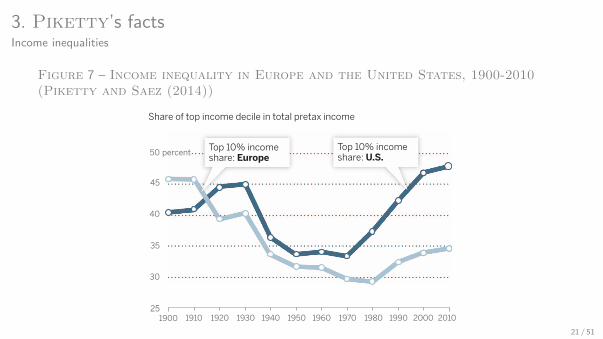
Figure 7 – Income inequality in Europe and the United States, 1900-2010(Piketty and Saez (2014))

REVIEW

Inequality in the long runThomas Piketty1* and Emmanuel Saez2

This Review presents basic facts regarding the long-run evolution of income and wealthinequality in Europe and the United States. Income and wealth inequality was very high acentury ago, particularly in Europe, but dropped dramatically in the first half of the 20thcentury. Income inequality has surged back in the United States since the 1970s so thatthe United States is much more unequal than Europe today. We discuss possibleinterpretations and lessons for the future.

The distribution of income and wealth is awidely discussed and controversial topic.Do the dynamics of private capital ac-cumulation inevitably lead to the con-centration of income and wealth in ever

fewer hands, as Karl Marx believed in the 19thcentury? Or do the balancing forces of growth,competition, and technological progress leadin later stages of development to reduced in-equality and greater harmony among the classes,as Simon Kuznets thought in the20th century? What do we knowabout how income and wealthhave evolved since the 18th cen-tury, and what lessons can we de-rive from that knowledge for thecentury now under way? For a longtime, social science research on thedistribution of income and wealthwas based on a relatively limitedset of firmly established facts to-gether with a wide variety of pure-ly theoretical speculations. In thisReview, we take stock of recentprogress that has been made inthis area. We present a numberof basic facts regarding the long-run evolution of income and wealthinequality in advanced countries.We then discuss possible inter-pretations and lessons for thefuture.

Data and Methods

Modern data collection on the dis-tribution of income begins in the1950s with the work of Kuznets (1).Shortly after having establishedthe first national income time seriesfor the United States, Kuznets sethimself to construct time series ofincome distribution. He used tab-ulated income data coming fromincome tax returns—available sincethe creation of the U.S. federal income tax in1913—and statistical interpolation techniques basedupon Pareto laws (power laws) to estimate incomes

for the top decile and percentile of the U.S.population. By dividing by national income,Kuznets obtained series of U.S. top income sharesfor 1913 to 1948.In the 1960s and 1970s, similar methods

using inheritance tax records were developed toconstruct top wealth shares (2, 3). Inheritancedeclarations and probate records dating backto the 18th and 19th centuries were also ex-ploited by a growing number of scholars in

France, the United States, and the United King-dom (4–7).Such data collection efforts on income and

wealth dynamics have started to become moresystematic and broader in scope and time onlysince the 2000s. This is due first to the adventof information technologies, which allow much

larger volumes of data to be collected and pro-cessed than were accessible to previous gener-ations of scholars. The second reason for thistime gap in using tax data is that most modernresearch on inequality has focused on micro-survey data that became available in the 1960sand 1970s in many countries. Survey data, how-ever, cannot measure top percentile incomesaccurately because of the small sample size andtop coding. The top percentile plays a very largerole in the evolution of inequality that we willdiscuss. Survey data also have a much shortertime span—typically a few decades—than taxdata that often cover a century or more.Kuznets-type methods to construct top in-

come shares were first extended and updated tothe cases of France (8, 9), the United Kingdom(10), and the United States (11). By combiningthe efforts of an international team of over 30scholars, similar series covering most of the20th century were constructed for more than25 countries (12–15). The resulting “World TopIncomes Database” (WTID) is the most ex-tensive data set available on the historicalevolution of income inequality. The series isconstantly being extended and updated and is

available online (http://topincomes.parisschoolofeconomics.eu/) asa research resource for furtheranalysis.Historical top wealth shares se-

ries have also been constructed withsimilar methods, albeit for a smallernumber of countries so far, but witha longer time frame (16–21). Draw-ing on previous attempts to collecthistorical national balance sheets(22), long-run series on the evolu-tion of aggregate wealth-incomeratios in the eighth largest devel-oped economies were established,some of them going back to the18th century (23).This Review draws extensively

on this body of historical researchon income and wealth, as well ason a recently published interpre-tive synthesis (24). We start bypresenting three basic facts thatemerge from this research pro-gram (Figs. 1 to 3), and then turnto interpretations.

Three Facts About Inequalityin the Long Run

We find large changes in the lev-els of inequality, both over timeand across countries. This re-flects the fact that economic trendsare not acts of God, and that

country-specific institutions and historical cir-cumstances can lead to very different inequalityoutcomes.

Income Inequality

First, we find that whereas income inequalitywas larger in Europe than in the United States a

1Department of Economics, Paris School of Economics, Paris,France. 2Department of Economics, University of Californiaat Berkeley, Berkeley, CA, USA.*Corresponding author. E-mail: thomas.piketty@psemail.eu

Top 10% incomeshare: Europe

Income inequality in Europe and the United States, 1900–2010 Share of top income decile in total pretax income

50 percent

45

40

35

30

25201020001990198019701960195019401930192019101900

Top 10% incomeshare: U.S.

Fig. 1. Income inequality in Europe and the United States, 1900 to 2010.The share of total income accruing to top decile income holders was higher inEurope than in the United States from 1900 to 1910; it was substantiallyhigher in the United States than in Europe from 2000 to 2010. The seriesreport decennial averages (1900 = 1900 to 1909, etc.) constructed usingincome tax returns and national accounts. See (24), chapter 9, Fig. 9.8. Seriesavailable online at piketty.pse.ens.fr/capital21c.

838 23 MAY 2014 • VOL 344 ISSUE 6186 sciencemag.org SCIENCE

21 / 51

3. Piketty’s factsIncome inequalities

I Whereas income inequality was larger in Europe than in the United States acentury ago, it is currently much larger in the United States.

I The top decile share in Europe is currently almost one-third smaller than what itused to be one century ago.

I The secular decline in inequality would be even larger if one takes into account therise of taxes and transfers, and measure instead income after taxes and transfers.

I Primary income concentration is currently higher than it has ever been in U.S.history. It is also slightly higher than in pre-WWI Europe.

22 / 51

3. Piketty’s factsWealth inequalities

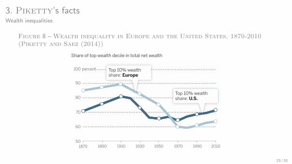
Figure 8 – Wealth inequality in Europe and the United States, 1870-2010(Piketty and Saez (2014))

century ago, it is currently much larger in theUnited States. This is true for every inequalitymetric. The simplest and most powerful measure,on which we focus in this article, is the share oftotal income going to the top decile (Fig. 1).On the eve of World War I (WWI), in the

early 1910s, the top decile income share wasbetween 45 and 50% of total income in mostEuropean countries. This applies in particularto the United Kingdom, France, Germany, andSweden, which are the four countries that weuse to compute the European average seriesreported in this article. At the same time, thetop decile income share was slightly above 40%in the United States.One century later, in the early 2010s, the in-

equality ordering between Europe and the UnitedStates is reversed. In Europe, the top decile in-come share fell sharply, from 45 to 50% to about30%, between 1914 and the 1950s–1960s. It hasbeen rising somewhat since the 1970s–1980s, andit is now close to 35% (somewhat less in con-tinental Europe and somewhat more in the UnitedKingdom, which has experienced an evolutioncloser to that of the United States). That is, thetop decile share in Europe is currently almostone-third smaller than what it used to be onecentury ago. The secular decline in inequalitywould be even larger if we took into account therise of taxes and transfers, and measure insteadincome after taxes and transfers. Total tax rev-enues and public spending were less than 10%of national income in every country before WWI,and they are now on the order of 30 to 50% ofnational income in every developed country. Prop-erly attributing taxes, transfers, andpublic spending to each income dec-ile raises important measurementissues, however, particularly regard-ing in-kind transfers (such as health,education, or public good spend-ing). In this Review, we thereforefocus on the long-run evolution ofthe inequality of primary income(pretax, pretransfer).In the United States, the top dec-

ile income share in 1910 was lowerthan in Europe, then rose in the1920s, fell in the 1930s–1940s, andstabilized around 30 to 35% in the1950s–1960s, slightly above Euro-pean levels of the time. It then roseat an unprecedented pace since the1970s–1980s, and is now close to50%. According to this measure, pri-mary income concentration is cur-rently higher than it has ever beenin U.S. history. It is also slightlyhigher than in pre-WWI Europe.

Wealth Inequality

Second, we observe the same “greatinequality reversal” between Europeand the United States when welook at wealth inequality rather thanincome inequality. That is, the shareof total net private wealth owned

by the top 10% of wealth holders was notablylarger in Europe than in the United States onecentury ago, while the opposite is true today(Fig. 2).There are important differences between in-

come and wealth inequality dynamics, how-ever. First, we stress that wealth concentrationis always much higher than income concen-tration. The top decile wealth share typicallyfalls in the 60 to 90% range, whereas the topdecile income share is in the 30 to 50% range.Even more striking, the bottom 50% wealthshare is always less than 5%, whereas the bot-tom 50% income share generally falls in the 20to 30% range. The bottom half of the popula-tion hardly owns any wealth, but it does earnappreciable income: On average, members ofthe bottom half of the population (wealth-wise)own less than one-tenth of the average wealth,while members of the bottom half of the pop-ulation (income-wise) earn about half the aver-age income.In sum, the concentration of capital ownership

is always extreme, so that the very notion ofcapital is fairly abstract for large segments—ifnot the majority—of the population. The inequal-ity of labor income can be high, but it is usuallymuch less extreme. It is also less controversial,partly because it is viewed as more merit-based.Whether this is justified is a highly complex anddebated issue to which we later return.Next, in contrast to income inequality, U.S.

wealth inequality levels have still not regainedthe record levels observed in Europe beforeWorld War I. The U.S. top decile wealth share

was about 70 to 80% in from 1870 to 1910, fell to60 to 70% from 1950 to 1980, and has beenrising above 70% in recent decades. Naturally,this means that wealth concentration has beenhigh throughout U.S. history. But this also impliesthat there has always been a large fraction of U.S.aggregate wealth—about 20 to 30%—that did notbelong to the top 10%. As the bottom 50% wealthshare has always been negligible, this remaining20 to 30% fraction corresponds to the shareowned by the “middle 40%” (i.e., the intermediategroup between the bottom 50% and the top 10%),a social group that one might want to call the“wealth middle class.” The important point isthat, to a large extent, there has always been awealth middle class in the United States.In contrast, wealth concentration was so ex-

treme in pre-WWI Europe that there was ba-sically no wealth middle class. That is, the topdecile wealth share was close to 90% (or evensomewhat higher than 90%, as in the UK), sothat the middle 40% wealth holders were almostas poor as the bottom 50% wealth holders (thewealth share of both groups was close to or lessthan 5%). Between 1914 and the 1950s–1960s, thetop decile wealth share fell dramatically in Eu-rope, from about 90% to less than 60%. It hasbeen rising since the 1970s–80s, and is now closeto 65% (somewhat more in the United Kingdom,and somewhat less in Continental Europe). Inother words, the wealth middle class now com-mands a larger share of total wealth in Europethan in the United States—although this sharehas been shrinking lately on both sides of theAtlantic.

Given that wealth inequality islower in the United States todaythan in 1913 Europe, why is U.S.income inequality now as large as(or even slightly larger than) thatin 1913 Europe? The reason is thatmodern U.S. inequality is basedmore on a very large rise of toplabor incomes than upon the ex-treme levels of wealth concentrationthat characterized the “patrimonial”(wealth-based) societies of the past.In 1913 Europe, top incomes werepredominantly top capital incomes(rent, interest, and dividends) com-ing from the very large concen-tration of capital ownership. TopU.S. incomes today are composedabout equally of labor income andcapital income. This generates ap-proximately the same level of totalincome inequality, but it is not thesame form of inequality.

Wealth-to-Income Ratios

Before further discussing the dif-ferent possible interpretations forthese important transformations,we introduce a third basic fact: Ifwe look at the evolution of the ag-gregate value of wealth relative toincome, we also find large historical

Wealth inequality in Europe and the United States, 1870–2010 Share of top wealth decile in total net wealth

100 percent

90

80

70

60

5020101990197019501930191018901870

Top 10% wealthshare: Europe

Top 10% wealthshare: U.S.

Fig. 2. Wealth inequality in Europe and the United States, 1870 to 2010.The share of total net wealth belonging to top decile wealth holders becamehigher in the United States than in Europe over the course of the 20thcentury. But it is still smaller than what it was in Europe before World War I.The series report decennial averages constructed using inheritance taxreturns and national accounts. See (24), chapter 10, Fig. 10.6. Series availableonline at piketty.pse.ens.fr/capital21c.

SCIENCE sciencemag.org 23 MAY 2014 • VOL 344 ISSUE 6186 839

23 / 51

3. Piketty’s factsWealth inequalities

I Same “great inequality reversal” between Europe and the United States when onelooks at wealth inequality rather than income inequality.

I However, important differences between income and wealth inequality dynamics.I Income versus wealth :

× wealth concentration is always much higher than income concentration.× the bottom 50% wealth share is always less than 5%, whereas the bottom 50%

income share generally falls in the 20 to 30% range

24 / 51

I US versus Europe

× In contrast to income inequality, U.S. wealth inequality levels have still not reachedthe record levels observed in Europe before World War I.

× Wealth concentration was extreme in pre-WWI Europe : the top decile wealth sharewas close to 90%, so that the middle 40% wealth holders were almost as poor as thebottom 50% wealth holders (the wealth share of both groups was close to or lessthan 5%) almost not middle class

× Between 1914 and the 1950s-1960s, the top decile wealth share fell dramatically inEurope, from about 90% to less than 60%. It has been rising since the 1970s–80s,and is now close to 65% . the wealth middle class now commands a larger shareof total wealth in Europe than in the United States.

× Given that wealth inequality is lower in the United States today than in 1913Europe, why is U.S. income inequality now as large as (or even slightly larger than)that in 1913 Europe ?

× Because modern U.S. inequality is based more on a very large rise of top laborincomes than upon the extreme levels of wealth concentration.

25 / 51

3. Piketty’s factsWealth-to-Income Ratios

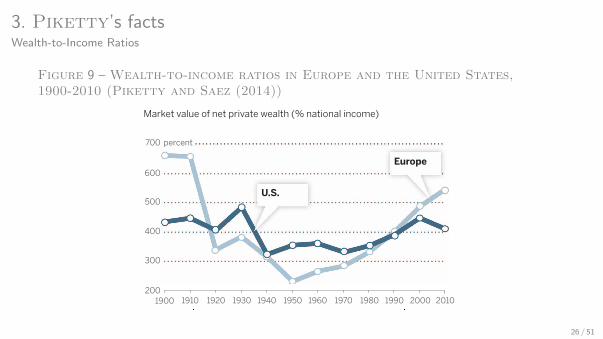
Figure 9 – Wealth-to-income ratios in Europe and the United States,1900-2010 (Piketty and Saez (2014))

variations, again with striking differences be-tween Europe and the United States (Fig. 3).This ratio is of critical importance for the anal-ysis of inequality, as it measures the overall im-portance of wealth in a given society, as well asthe capital intensity of production.In every European country for which we have

data, and in particular France, the United King-dom, and Germany, the aggregate wealth-incomeratio has followed a pronounced U-shaped pat-tern over the past century. On the eve of WWI,net private wealth was about equal to 6 to 7 yearsof national income in Europe. It then fell toabout 2 to 3 years of national income in the1950s. It has risen regularly since then, and it isnow back to about 5 to 6 years of national in-come. Interestingly, we also find a similar pat-tern for Japan (23).In contrast, the U.S. pattern is flatter: Net pri-

vate wealth has generally equalled about 4 to5 years of national income in the United States,with much less variation than in Europe or Japan.The U.S. pattern is also slightly U-shaped—withaggregate wealth-income ratios standing at arelatively lower level in the mid-20th centurythan at both ends of the century. But it is clearlymuch less marked than in Europe.The comparison between Figs. 1 and 3 is

particularly striking. Both figures have twoU-shaped curves, but these are clearly differ-ent. The United States displays a U-shapedpattern for income inequality (mostly drivenby the large rise of top labor incomes in recentdecades). Europe (and Japan) shows a U-shapedpattern for aggregate wealth-income ratios.The United States is the land of booming toplabor incomes; Europe is the landof booming wealth (albeit with alower wealth concentration thanin the United States). These aretwo distinct phenomena, involv-ing different economic mechanismsand different parts of the devel-oped world.

Interpreting theLong-Run Evidence

We now turn to the discussion ofpossible interpretations and les-sons for the future. We stress at theoutset that what we have to offer islittle more than an informed dis-cussion. Although we have at ourdisposal much more extensive his-torical and comparative data thanwere available to previous research-ers, existing evidence is still far tooincomplete and imperfect for a rig-orous quantitative assessment ofthe various causes at play. Severaldifferent mechanisms have clear-ly played an important role in theevolution of income and wealthdepicted in Figs. 1 to 3, but it isextremely difficult to disentanglethe individual processes. We arenot in the domain of controlled

experiments: We cannot replay the 20th-centuryincome and wealth dynamics as if the world wars,the rise of progressive taxation, or the Bolshevikrevolution did not happen. Still, we can try tomake some progress.

Wealth-to-Income Ratios

The relatively easier part of the story is the long-run evolution of aggregate wealth-to-income ra-tios (Fig. 3). The fall of European wealth-incomeratios following the 1914–1945 capital shocks canbe well accounted for by three main factors: directwar-related physical destruction of domestic capitalassets (real estate, factories, machinery, equipment);lack of investment (a large fraction of 1914–1945private-saving flows was absorbed by the enor-mous public deficits induced by war financing;there was also massive dissaving in some cases,e.g., foreign assets were sold to purchase gov-ernment bonds; the resulting public debt waseventually wiped away by inflation); and a fall inrelative asset prices (real estate and stock mar-ket prices were both historically very low in theimmediate postwar period, partly due to rentcontrol, nationalization, capital controls, andvarious forms of financial repression policies).In France and Germany, each of these threefactors seems to account for about one-third ofthe total decrease in wealth-income ratios. Inthe United Kingdom, where domestic capitaldestruction was of limited importance (less than10% of the total), the other two factors eachaccount for about half of the decline in the ag-gregate wealth-income ratio (23, 24).Why did the postwar recovery of European

wealth-income ratios take so much time? The

simplest way to understand why capital accu-mulation is a slow process is to consider thefollowing elementary arithmetic: With a savingrate of 10% per year, it takes 50 years to accu-mulate the equivalent of 5 years of income.How is the long-run equilibrium wealth-income

ratio determined, and why does it seem to vary acrosscountries and over time? A simple yet powerfulway to think about this issue is the so-calledHarrod-Domar-Solow formula (23). In the long-run, assuming no systematic divergence betweenthe relative price of capital assets and consumptiongoods, one can show that the wealth-to-income(or capital-to-income) ratio bt = Kt/Yt convergestoward b = s/g, where s is the long-run annualsaving rate and g is the long-run annual totalgrowth rate. The growth rate g is the sum of thepopulation growth rate (including immigration)and the productivity growth rate (real incomegrowth rate per person). This formula holdswhether savings are invested in domestic orforeign assets (it also holds at the global level).That is, with a saving rate s = 10% and a growth

rate g = 3%, then b ≈ 300%. But if the growthrate drops to g = 1.5%, then b ≈ 600%. In short:Capital is back because low growth is back.Intuitively, in a low-growth society, the to-

tal stock of capital accumulated in the pastcan become very important. In the extremecase of a society with zero population and pro-ductivity growth, income Y is fixed. As long asthere is a positive net saving rate s > 0, thequantity of accumulated capital K will go toinfinity. Therefore, the wealth-income ratiob = K/Y would rise indefinitely (at some point,people in such a society would probably

stop saving, as additional capi-tal units become almost useless).With positive but small growth,the process is not as extreme:The rise of b stops at some finitelevel. But this finite level can bevery high.One can show that this simple

logic can account relatively wellfor why the United States accumu-lates structurally less capital relativeto its annual income than Europeand Japan. U.S. population growthrates exceed 1% per year, thanksto large immigration flows, so totalU.S. growth rates—including pro-ductivity growth of around 1 to1.5%—are at least 2 to 2.5% peryear, if not 2.5 to 3%. By contrast,population growth in Europe andJapan is now close to zero, so thattotal growth is close to produc-tivity growth, i.e., about 1 to 1.5%per year. This is further reinforcedby the fact that U.S. saving ratestend to be lower than in Europeand Japan. To the extent that pop-ulation growth will eventually de-cline almost everywhere, and thatsaving rates will stabilize, this al-so implies that the return of high

Wealth-to-income ratios in Europe and the United States, 1900–2010 Market value of net private wealth (% national income)

700 percent

600

500

400

300

200201020001990198019701960195019401930192019101900

U.S.

Europe

Fig. 3. Wealth-to-income ratios in Europe and the United States, 1900 to2010.Total net private wealth was worth about 6 to 7 years of national incomein Europe before World War I, fell to 2 to 3 years in 1950–1960, and increasedback to 5 to 6 years in 2000–2010. In the United States, the U-shape patternwas much less marked. The series report decennial averages (1900 = 1900 to1909, etc.) constructed using national accounts. See (24), chapter 5, Fig. 5.1.Series available online at piketty.pse.ens.fr/capital21c.

840 23 MAY 2014 • VOL 344 ISSUE 6186 sciencemag.org SCIENCE

26 / 51

3. Piketty’s factsWealth-to-Income Ratios

I Europe aggregate wealth-income ratio : U-shaped pattern over the past century :

× Eve of WWI, net private wealth was about equal to 6 to 7 years of national income× Fall to about 2 to 3 years of national income in the 1950s.× Regular increase since then, back to about 5 to 6 years of national income.

I In contrast, the U.S. pattern is flatter, around 4 to 5 years of national income

I The United States is the land of booming top labor incomes ; Europe is the landof booming wealth.

27 / 51

3. Piketty’s factsHistorical interpretation

I Fall of European wealth-income ratios caused by three main factors :

× direct war-related physical destruction of domestic capital assets (real estate,factories, machinery, equipment)

× lack of investment (a large fraction of 1914–1945 private-saving flows was absorbedby the public deficits induced by war financing)

× fall in relative asset prices (real estate and stock market prices were both historicallyvery low in the immediate postwar period, partly due to rent control, nationalization,capital controls, and various forms of financial repression policies).

I France and Germany : each of these three factors seems to account for aboutone-third of the total decrease in wealth-income ratios

I UK : domestic capital destruction is less than 10% of the total), the other twofactors each account for about half each.

28 / 51

3. Piketty’s factsHistorical interpretation

I Why was the rise of European wealth-income ratios slow after WWII ?

I Because capital accumulation is a slow process :

I With a saving rate of 10% per year, it takes 50 years to accumulate the equivalentof 5 years of income.

29 / 51

4. Piketty’s two ”laws of capitalism”Piketty’s view about the long run

I “First law of capitalism” (actually an identity) :

σk = r × k

y

I “Second law of capitalism” : if the saving rate s is constant and g is the growthrate of the economy :

k

y=

s

g

When growth goes to zero, capital becomes arbitrarily bigger that income.

I Those two laws imply σk = s rg

I If g drops while r does not much, then the share of capital in total incomebecomes very large we shall expect a lot of inequalities ...

I As indeed r > g (see Figure 10), capital taxes are needed if one dislike inequalities(now we are on a normative ground)

30 / 51

4. Piketty’s two ”laws of capitalism”r > g ?

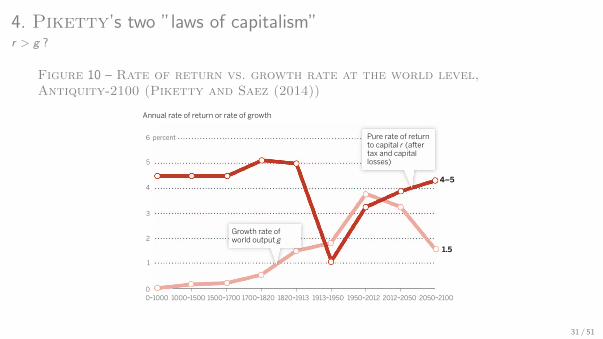
Figure 10 – Rate of return vs. growth rate at the world level,Antiquity-2100 (Piketty and Saez (2014))

capital-to-income ratios will apply at the globallevel in the very long run (23, 24).The share of capital income in national in-

come is defined as a = rK/Y = rb, where r is theaverage annual real rate of return on wealth.For instance, if r = 5% and b = K/Y = 600%, thena = 30%. Whether the rise in the capital incomeratio b will also lead to a rise in a is a compli-cated issue.In the standard economic model with per-

fectly competitive markets, r is equal to themarginal product of capital (that is, the addi-tional output produced by one additional cap-ital unit, all other things being equal). As thevolume of capital b rises, the marginal productr tends to decline. The important question iswhether r falls more or less rapidly than therise in b. This depends on what economists de-fine as the elasticity of substitution s betweencapital and labor in the production functionY = F(K, L).A standard hypothesis in economics has been

to assume a unitary elasticity, in which case thefall in r exactly offsets the rise in b, so that thecapital share a = rb is a technological constant.However, historical variations in capital sharesare far from negligible: a typically varies in the20 to 40% range (and the labor share 1 – a in the60 to 80% range). In recent decades, rich coun-tries have experienced both a rise in b and a risein a, which suggests that s is somewhat largerthan 1. Intuitively, it makes sense to assume thats tends to rise over the development process, asthere are more diverse uses and forms for capitaland more possibilities to substitute capital forlabor (e.g., replacing delivery workers by dronesor self-driving trucks).Whether the capital share a will keep rising

in future decades is an open question. It de-pends both on technological forces and on thebargaining power of capital and labor and thecollective institutions regulating the capital-labor relationship (the simple economic mod-el with perfectly competitive markets is likelyexcessively naïve). But from a logical standpoint,this is a plausible possibility, especially if thepopulation and productivity growth slowdownpushes the global capital income ratio b towardhigher levels.

Wealth Inequality: r > g

We now move to an even more complicated—andarguably more important—issue: the long-run dy-namics of wealth inequality (Fig. 2). High capitalintensity, as measured by high b and a, is not badin itself. After all, it would be good to have aninfinite quantity of robots producing most of theoutput, so that we can devote more time to leisureactivities. The problem is twofold: Can we all findjobs as a robot designer (or in leisure-related ac-tivities), and who owns the robots? In practice,the concentration of capital ownership alwaysseems to be very high—much more than the con-centration of labor income (Figs. 1 and 2). The“patrimonial” (wealth-based) societies of Europeone century ago were characterized not only byvery high b and a, but also by extreme capital

concentration, with a top decile wealth share ofaround 90%.How can we account for the very high level of

wealth concentration that we observe in histor-ical series, and what does this tell us about thefuture? The most powerful model to analyze struc-tural changes in wealth inequality is a dynamicmodel with multiplicative random shocks. That is,assume that the individual-level wealth processhas the following general form: zit+1 = witzit + eit,where zit is the position of individual i in thewealth distribution prevailing at time t (i.e., zit =kit/kt where kit is net wealth owned by individ-ual i at time t, and kt = average net wealth ofthe entire population at time t), wit is a multi-plicative random shock, and eit is an additiverandom shock.The shocks wit and eit can be interpreted as

reflecting different types of events that oftenoccur in individual wealth histories, includingshocks to rates of return (some individuals mayget returns that are far above average returns;investment strategies may fail and lead to fam-ily bankruptcy); shocks to demographic param-eters (some families have many children; someindividuals die young); shocks to preferencesparameters (some individuals like to save, someprefer to consume their wealth); shocks to pro-ductivity parameters (capital income is sometimes

supplemented by high labor income); and so on.Importantly, for a given structure of shocks,

the variance of the multiplicative term wit is anincreasing function of r – g, where r is the (net-of-tax) rate of return and g is the economy’s growthrate. Intuitively, a higher r – g tends to amplifyinitial wealth inequalities: It implies that pastwealth is capitalized at a faster pace, and that it isless likely to be overtaken by the general growthof the economy. Under fairly general conditions,one can show that the top tail of the distributionof wealth converges toward a Pareto distribution,and that the inverted Pareto coefficient (measur-ing the thickness of the upper tail and hence theinequality of the distribution) increases with r – g(3, 14, 24–26).The dynamic wealth accumulation model with

multiplicative shocks can explain the extremelevels of wealth concentration that we observe inthe data much better than alternative models. Inparticular, if wealth accumulation were predomi-nantly driven by lifecycle or precautionary mo-tives, then wealth inequality would not be as largeas what we observe (it would be comparable inmagnitude to income inequality, or even lower).The dynamic multiplicative model can also

help to explain some of the important historicalvariations that we observe in wealth concentra-tion series.

1.5

4–5

Rate of return vs. growth rate at the world level, Antiquity–2100 Annual rate of return or rate of growth

6 percent

4

5

2

3

01000-1500 1500-1700 1700-1820 1820-1913 1913-1950 1950-2012 2012-2050 2050-21000-1000

1

Pure rate of return to capital r (after tax and capital losses)

Growth rate of world output g

Fig. 4. Rate of return versus growth rate at the global level, from Antiquity until 2100. Theaverage rate of return to capital (after tax and capital losses) fell below the growth rate in the 20thcentury. It may again surpass it in the 21st century, as it did throughout human history except in the20th century. The series was constructed using national accounts for 1700 and after and historicalsources on growth and rent to land values for the period before 1700. See (24), chapter 10, Fig. 10.10.Series available online at piketty.pse.ens.fr/capital21c. The future values for g are based upon UNdemographic projections (median scenario) for population growth and on the assumption thatbetween-country convergence in productivity growth rates will continue at its current pace. Thefuture values for r are simply based upon the continuation of current pretax values and the assump-tion that tax competition will continue. See (24), chapter 10, Fig. 10.10. Series available online atpiketty.pse.ens.fr/capital21c.

SCIENCE sciencemag.org 23 MAY 2014 • VOL 344 ISSUE 6186 841

31 / 51

4. Piketty’s two ”laws of capitalism”Piketty and Solow

I This view that capital income could absorb all come when g goes to zero seems tocontradict what we know from balanced growth in the Solow model, that is theexistence of a Balanced Growth Path.

I More specifically, going back to the two laws of capitalism :

32 / 51

4. Piketty’s two ”laws of capitalism”Second law

I The second law states :k

y=

s

g

× Is that reasonable to assume that s stays constant ?× Are we talking about net output or gross output ?× The distinction is important

ynet = ygross − δk

× When k becomes large, δk also becomes large.

33 / 51

4. Piketty’s two ”laws of capitalism”First law

I First law states :

σk = r × k

y

× We know that if the production function is Cobb-Douglas y = Akα`1−α, thenσk = α.

× This means that when ky increases by 1%, r decreases by 1%.

× Is that reasonable to assume that r does not decrease (or do not decrease a lot)when k

y increases ?× We will show that this depends on the elasticity of substitution between capital and

labor.

34 / 51

4. Piketty’s two ”laws of capitalism”Questions

I We will first discuss on the assumption under which ky becomes arbitrarily large

when g goes to 0.

I We then discuss the role of the elasticity of substitution between capital and labor.

35 / 51

5. ky in the Solow model and beyond

The Solow model

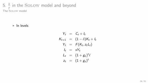
I In levels

Yt = Ct + It

Kt+1 = (1 − δ)Kt + It

Yt = F (Kt , ztLt)

It = sYt

Lt = (1 + gL)t`

zt = (1 + gz)t

36 / 51

5. ky in the Solow model and beyond

The Solow model

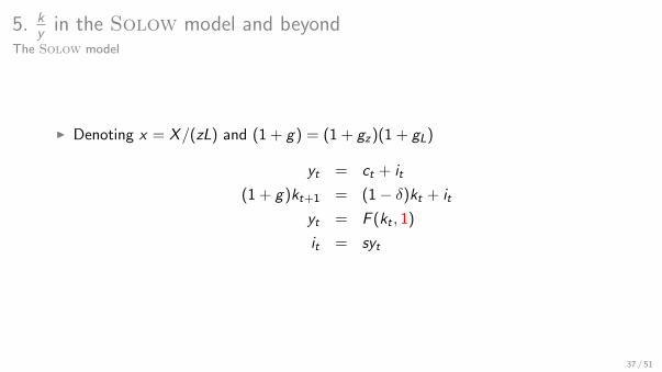
I Denoting x = X/(zL) and (1 + g) = (1 + gz)(1 + gL)

yt = ct + it

(1 + g)kt+1 = (1 − δ)kt + it

yt = F (kt , 1)

it = syt

37 / 51

5. ky in the Solow model and beyond

The Solow model

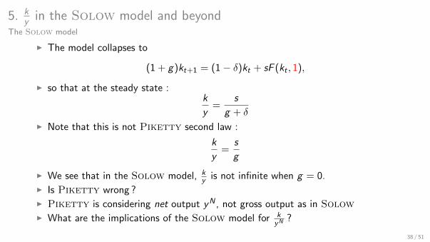
I The model collapses to

(1 + g)kt+1 = (1 − δ)kt + sF (kt , 1),

I so that at the steady state :k

y=

s

g + δ

I Note that this is not Piketty second law :

k

y=

s

g

I We see that in the Solow model, ky is not infinite when g = 0.

I Is Piketty wrong ?I Piketty is considering net output yN , not gross output as in SolowI What are the implications of the Solow model for k

yN ?

38 / 51

5. ky in the Solow model and beyond

Net and gross accounting

I Define net output as yN = y − δk

I Piketty assumption is that investment is a constant fraction of net output.

I In Piketty, it is the net saving rate sN that is constant, whereas it is the grossone s in Solow.

I Does it make a difference ?

I What is the implication of the Solow model for sN ?

I What is the dynamics of the Solow model when sN is constant instead of s ?

39 / 51

5. ky in the Solow model and beyond

Net and gross accounting

I Define net output as yN = y − δk

I Piketty assumption is that investment is a constant fraction of net output.

I In Piketty, it is the net saving rate sN that is constant, whereas it is the grossone s in Solow.

I Does it make a difference ?

I What is the implication of the Solow model for sN ?

I What is the dynamics of the Solow model when sN is constant instead of s ?

40 / 51

5. ky in the Solow model and beyond

The two laws of capitalism again

I With our notations, Piketty’s laws are

σNk = r × k

yN

andk

yN=

sN

g

41 / 51

5. ky in the Solow model and beyond

The net saving rate in Solow

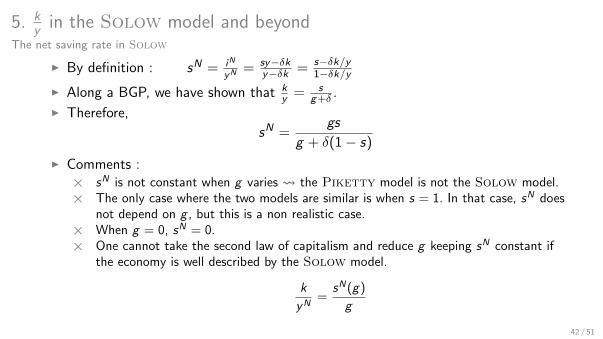
I By definition : sN = iN

yN = sy−δky−δk = s−δk/y

1−δk/yI Along a BGP, we have shown that k

y = sg+δ .

I Therefore,

sN =gs

g + δ(1 − s)

I Comments :× sN is not constant when g varies the Piketty model is not the Solow model.× The only case where the two models are similar is when s = 1. In that case, sN does

not depend on g , but this is a non realistic case.× When g = 0, sN = 0.× One cannot take the second law of capitalism and reduce g keeping sN constant if

the economy is well described by the Solow model.

k

yN=

sN(g)

g

42 / 51

5. ky in the Solow model and beyond

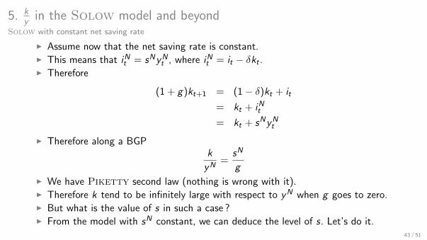
Solow with constant net saving rate

I Assume now that the net saving rate is constant.I This means that iNt = sNyNt , where iNt = it − δkt .I Therefore

(1 + g)kt+1 = (1 − δ)kt + it

= kt + iNt

= kt + sNyNt

I Therefore along a BGPk

yN=

sN

g

I We have Piketty second law (nothing is wrong with it).I Therefore k tend to be infinitely large with respect to yN when g goes to zero.I But what is the value of s in such a case ?I From the model with sN constant, we can deduce the level of s. Let’s do it.

43 / 51

5. ky in the Solow model and beyond

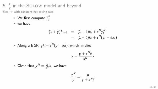
Solow with constant net saving rate

I We first compute yN

y

I we have

(1 + g)kt+1 = (1 − δ)kt + sNyNt

= (1 − δ)kt + sN(yt − δkt)

I Along a BGP, gk = sN(y − δk), which implies

y =g + sNδ

sNk

I Given that yN = gsNk , we have

yN

y=

g

g + sNδ

44 / 51

5. ky in the Solow model and beyond

Solow with constant net saving rate

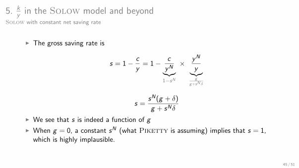
I The gross saving rate is

s = 1 − c

y= 1 − c

yN︸︷︷︸1−sN

× yN

y︸︷︷︸g

g+sNδ

s =sN(g + δ)

g + sNδ

I We see that s is indeed a function of g

I When g = 0, a constant sN (what Piketty is assuming) implies that s = 1,which is highly implausible.

45 / 51

6. The elasticity of substitution between k and `Back to σk

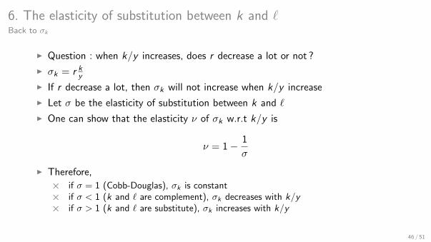
I Question : when k/y increases, does r decrease a lot or not ?

I σk = r kyI If r decrease a lot, then σk will not increase when k/y increase

I Let σ be the elasticity of substitution between k and `

I One can show that the elasticity ν of σk w.r.t k/y is

ν = 1 − 1

σ

I Therefore,

× if σ = 1 (Cobb-Douglas), σk is constant× if σ < 1 (k and ` are complement), σk decreases with k/y× if σ > 1 (k and ` are substitute), σk increases with k/y

46 / 51

6. The elasticity of substitution between k and `Back to σk

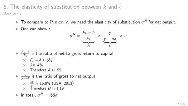
I To compare to Piketty, we need the elasticity of substitution σN for net output.

I One can show :

σN =Fk − δ

Fk︸ ︷︷ ︸A

× y

y − δk︸ ︷︷ ︸B

× σ

I Fk−δFk

is the ratio of net to gross return to capital.

× Fk − δ ≈ 5%× δ ≈ 4%× Therefore A ≈ .55

I yy−δk is the ratio of gross to net output

× δky ≈ 15.8% (USA, 2013)

× Therefore B ≈ 1.19

I In total, σN = .66σ

47 / 51

6. The elasticity of substitution between k and `Back to σk

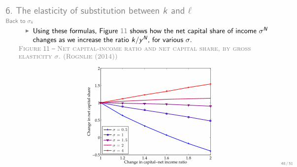
I Using these formulas, Figure 11 shows how the net capital share of income σN

changes as we increase the ratio k/yN , for various σ.Figure 11 – Net capital-income ratio and net capital share, by grosselasticity σ. (Rognlie (2014))

Figure 1: Relationship between net capital-income ratio and net capital share, by grosselasticity s.

1 1.2 1.4 1.6 1.8 2−0.5

0

0.5

1

1.5

2

Change in capital−net income ratio

Ch

ang

e in

net

cap

ital

sh

are

σ = 0.5

σ = 1

σ = 1.5

σ = 2

σ = 4

2.4 Empirical literature on the elasticity of substitution

Ever since Arrow, Chenery, Minhas and Solow (1961) first proposed the constant elasticityof substitution (CES) production function, researchers have attempted to estimate the keyelasticity parameter s. These studies have virtually always looked at the elasticity ofsubstitution in the gross production function.

The literature is vast and its conclusions muddled, but one consistent theme has beenthe rarity of high elasticity estimates. Chirinko (2008) provides an excellent summaryof the empirical literature, listing estimates from many different sources and empiricalstrategies. Of the 31 sources6 listed for the gross elasticity, fully 30 out of 31 show sgross <2. 29 out of 31 show sgross < 1.5, and 26 out of 31 show sgross < 1. The median issgross = 0.52, and Chirinko concludes that “the weight of the evidence suggests that sgross

lies in the range between 0.40 and 0.60”. Table 1 shows the full distribution.Figure 1 shows the implications of this rough consensus value of sgross = 0.5. As

discussed above, given this value even small increases in the capital-output ratio K/Ynet

lead to a plummeting net capital share. Even with sgross = 1, which is higher than over80% of the estimates listed in Chirinko (2008), Figure 1 indicates that the net capital sharefalls substantially when the capital-output ratio rises. A gross elasticity of sgross = 2,

6For a few sources that list a range of elasticities, I take the midpoint. This has minimal effect on thedistribution.

7

48 / 51

6. The elasticity of substitution between k and `Back to σk

I In the data, it is hard to find estimates of σ that are larger than 2.

I Therefore, for plausible σ, an increase in k/y does not lead to a big increase inthe capital income share in the long run (and likely a decline)

49 / 51

7. Summary

I News set of fact brought by Piketty about income distribution

I We observe an increase in income inequalities and wealth-to-income ratios

I Piketty extrapolates an explosion of k/y and inequalities when r > g and g low.

I Using the Solow model with constant net saving rate or constant saving rate, thisis unlikely.

I Using reasonable estimates of elasticity of substitution between k and `, it is alsounlikely.

I This does not mean that inequalities are at the right level (to be defined), notthat they cannot stay high for a long period (but not along a BGP).

50 / 51

8. References

I Krusell, Per and Anthony Smith, “Is Piketty’s “Second Law of Capitalism”Fundamental ?”, working paper, 2014

I Piketty, Thomas, “Capital in the Twenty-First Century”, Harvard University Press,2014

I Piketty, Thomas and Emmanuel Saez, “Inequality in the long run”, Science, Vol.244 Iss. 6186, 2014

I Rognlie, Matthew, “A note on Piketty and diminishing returns to capital”,working paper, 2014

I Sandra, Agnar, “The Principal Problem in Political Economy : IncomeDistribution in the History of Economic Thought”, working paper, 2013

51 / 51