2016,Problem B

Commercial Strategy for Addressing OrbitDebris Problem as A Private Firm

February 8, 2016

1

Control Number 54097

Contents

1 Introduction 3

2 Problem Statement 4

2.1 Definition of space debris . . . . . . . . . . . . . . . . . . . . . . . . . . . . . . 4

2.2 Effect of space debris . . . . . . . . . . . . . . . . . . . . . . . . . . . . . . . . . 4

2.3 Theoretical Backgrounds . . . . . . . . . . . . . . . . . . . . . . . . . . . . . . . 5

3 The space junk removal concept 5

4 Economic Analysis of Space Junk Removal Program 7

5 VaR Analysis of Orbits 8

5.1 Deduced Value of Orbits . . . . . . . . . . . . . . . . . . . . . . . . . . . . . . . 8

5.2 Cost-Benefit Analysis . . . . . . . . . . . . . . . . . . . . . . . . . . . . . . . . . 10

5.3 Comment . . . . . . . . . . . . . . . . . . . . . . . . . . . . . . . . . . . . . . . 10

6 Cost Estimation Technique 10

6.1 Estimated cost per kg deorbited . . . . . . . . . . . . . . . . . . . . . . . . . . . 11

6.2 Estimate Cost per Mission . . . . . . . . . . . . . . . . . . . . . . . . . . . . . . 11

6.3 Advanced Missions Cost Model Brady Kalb . . . . . . . . . . . . . . . . . . . . 11

6.4 Cost Estimation Results . . . . . . . . . . . . . . . . . . . . . . . . . . . . . . . 12

6.5 Comments . . . . . . . . . . . . . . . . . . . . . . . . . . . . . . . . . . . . . . . 13

7 Sensitive Analysis of the profit 13

8 Conclusion 14


Abstract

In this report, we embark on finding the most efficient strategy or combinationof strategies of the space junk Removal program using VaR Analysis and CostEstimation Technique. Above all, there are some commercial opportunitiesin this area after the logical economic analysis of this program. Moreover,some mature and available methods can be used here as the solid technologicalbackground to run this project. After searching and analysing data from officialorganization using our models, the costs and benefits can be approximatelyestimated respectively as the items of final profit model. Although there arequit expensive for the equipment and it seems impossible at the moment, thecost will be reduced along with the development of the relevant technique.This program can generate considerable benefit from our analysis of models. Inconclusion, we recommend private firm to consider running this program as along-term commercial program.

1 Introduction

In 2010, the U.S. President Barack Obamas National Space Policy was pub-lished. It simply directs NASA and the Defense Department to perform re-search and development of technologies and techniques to mitigate and remove


on-orbit debris, reduce hazards, and increase understanding of the current andfuture debris environment[12]. In June 2014, NASA adopted a policy to sup-port development of orbital debris removal technology. According to NASAspokesman Joshua Buck in an emailed response to a question about the policyon June 8, there is no viable technological or economically affordable approachthat is sufficiently mature to justify technology demonstration at present[3].

In Switzerland, engineers at the cole Polytechnique Fdrale de Lausanne are de-signing Clean Space One, a spacecraft to catch a cubesat and move it to Earthsatmosphere. Astroscale, a startup based in Singapore, is preparing to launch adual-satellite Active Debris Removal System in 2017. The German AerospaceCenter, DLR, plans to begin servicing spacecraft in orbit and removing debristhrough its Deutsche Orbital Servicing Mission scheduled to launch in 2018[12].

In this report, we are going to evaluate the economic viability of the devel-oping SOLDIER vehicle project. The concept of the project and the principlehow the SOLDIER vehicle works are included at first. Then, the Value at RiskModel and Advanced Mission Cost Model are employed to check the benefitand the cost of the project respectively[8]. Furthermore, a sensitive analysis ofthe whole profit is performed to show the viability.

2 Problem Statement

2.1 Definition of space debris

The collection of defunct artificial objects in orbit around Earth is called spacedebris such as old satellites, exhausted rocket stages, and fragments from dis-integration, erosion, and collisions including those caused by debris itself.

NASA (the National Aeronautics and Space Administration) defines space de-bris as all man-made objects in orbit about the Earth which no longer serve auseful purpose[13].

2.2 Effect of space debris

A small piece of space debris could blow the satellite into thousands of frag-ments, due to the huge energy, which is released during the process when debriswith high velocities crashes satellite. After such an accident, a thousand piecesof debris will be generated, which increases the probabilities of occurrence ofsuch potential crash events[2]. Although these pieces of debris will be clustered


at the beginning, overtime, they will disperse due to the regression of node.After the impact of the gravitational force from sun, moon and earth, and theywill almost completely encircle the earth within one year; which implies theworldwide risk caused by the fragmentation event[11].

2.3 Theoretical Backgrounds

The Six Kepler Elements:In order to define the position and velocity for the space object, it is normalto use set of orbital parameters. We will use the six Kepler elements in oursimulation: a: the semimajor axis;e: the eccentricity;i: the inclination;Ω The right ascension of ascending node;ω : The argument of perigee;M: the mean anomaly[11].

Kepler’s LawsIn astronomy, Keplers laws of planetary motion are three scientific laws describ-ing the motion of planets around the sun. The orbit of a planet is an ellipsewith the sun at one of the two foci. A line segment joining a planet and thesun sweeps out equal areas during equal intervals of time. The square of theorbital period of a planet is proportional to the cube of the semi-major axis ofits orbit[4].

The Classical Equation For Kinetic EnergyIn this model, the classical equation for kinetic energy for the satellite indicatedby the space junk is as follow:

Ek =1

2mSDv

2pas (1)

where Ek[J ] is the kinetic energy, mSD is the mass of the Space Debris, andvpas is the speed between the satellite and the space debris.

3 The space junk removal concept

The risk of orbital debris has been highlighted as a major forthcoming issue forspace vehicle safety and operations. According to NASA, five derelict satellitesmust be safely removed from low Earth orbit (LEO) every year in order to keepthe risk of orbital debris from escalating. To solve this problem, SOLDIER


was designed as a concept vehicle to respond to these growing needs[5]. TheSOLDIER vehicle is a small one-time use satellite, which is launched to targeta single derelict satellite, performs close proximity operations around the targetsatellite, attaches to the target using a tethered lance and then re-enters withthe attached target to dispose of it safely[6]. This section will cover the gen-eral design of the SOLDIER concept and its primary functionality as a ’largecategory orbital debris remover’. At the same time, the issue of capturing therotating targets will be investigated.

The SOLDIER concept was developed to remove large size space junks such asspacecraft and large remains of launch operations or in-orbit breakups. Sincethere are still lots of small size space junks, it can not solve the problem of orbitdebris completely[6]. However, it can be applied to the area of the problem witha high benefit to-cost ratio. In this way, this concept may not only be a goodapproach for the governments but also could become an economically viablebusiness case. Once the large size space junks are removed, it will effectivelyreduce the risk of collision of large size space junks. Hence, it will reduce theamount of the small size space junks generated by collision which are hard todetect and remove[6]. From this aspect, there are considerable benefits in thelong term.

This part will move on to show how this SOLDIER vehicle works. The SOL-DIER vehicle uses a tethered lance or harpoon to catch the target. A simplesimulation of the capture will be carried out in the following context[6].

Parameters denoted:θ1= Yaw angle between cable and target capture planeθ2= Pitch angle between cable and target capture planeω1=Yaw rateω2=Pitch rateH1=Yaw component target momentumH2=Pitch component target momentumFT = Force on targetrt = Distance from target center of gravity to capture pointI = Target moment of inertia

Assumption1. The capture mechanism is connected securely and it hits the target.2. Thrusters are actuated immediately upon contact (the cable is always under


tension)3. The SOLDIER vehicle is controlled to be relatively stationary to the targetdebris.4. The target is a cube with evenly distributed mass and the rotation aboutthe axis of the cable is ignored.

4H1

4H2

= cos

θ1

θ2

FTrt (2)

ω1

ω2

=

H1

H2

/I (3)

4θ1

4θ2

= cos

ω1

ω2

(4)

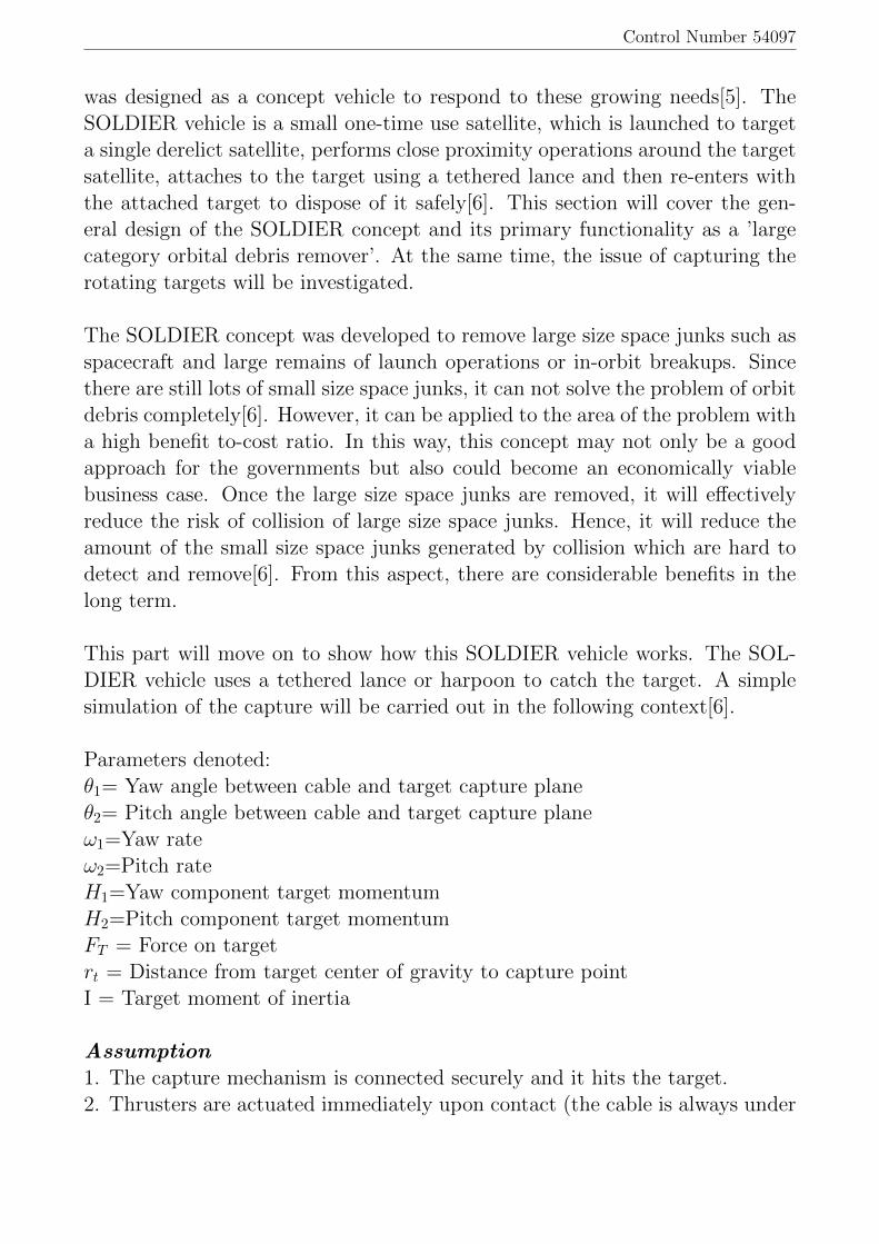
The equations above represent the dynamic model showing that the force actsoppositely to the direction of rotation as a corrective or stabilizing force. Thepurpose of the simulation is to show that the angular momentum of the targetdebris can be controlled via this cable under tension[3]. Because the modelis simple, a simple controller (proportional momentum controller) is used tothrottle the thrust and damp the momentum.We want to show the simulated cable angle from normal with debris target overthe first 30 minutes of capture. (simulation outcome)

4 Economic Analysis of Space Junk Removal Program

Figure 1


In the wake of developments in science and technology, the amount of thelaunched spacecraft increases rapidly, bringing about 300,000 pieces of debriswhich has enough size to destroy the satellite[8]. While insurance fees can beused as reference for this project, the insurance premium against space riskwas up to $800 million in 2011 and losses due to damage valued $600 million.Based on this situation, there may be some economic opportunities for privatefirm to dig out new profit target[1]. In this section, we will analyse the valueof this potential commercial opportunity, and conclude some efficient strategyor combination of strategies for private company to make profits in space junkremoval Program.

The purpose of this report is to dig out the possible maximum profits of SpaceJunk Removal Program by considering expected cost and benefit under possi-ble risk conditions. Since this program aims to eliminate the possible threatof satellites, then the profits are achieved from the revenue of the global satel-lite revenue in 2014, which valued totally $195.2 billion[1]. By considering thepossible risk percentage and the global satellites’ revenue, the benefit can beestimated and predicted by using following models based on the past severalyears’ data.

Next step is to minimize the cost of our mission. It’s conventional wisdomthat there are three orbits including Low Earth orbit (LEO) with altitudesup to 2,000 km, Medium Earth orbit (MEO) with altitudes from 2,000 km to35,786 km, and High Earth orbit above the altitude of geosynchronous orbit.Since the majority of satellites circled around LEO, it’s efficient just to considerremoving space junk with short distance from earth surface. From this aspect,the cost can be reduced and the profit can be increased[10]. As for the followingsections, the models are established only for orbit debris in LEO.

5 VaR Analysis of Orbits

5.1 Deduced Value of Orbits

It’s a conventional wisdom that the cost of active removal for orbital junk isreally expensive, and the debris is useless. Based on the futility of debris itself,the risk of its removal and reduction missions seem significant to be considered.The focus here is not who is the purchaser here, however, space systems com-


panies, government and inter-governmental agencies, and insurance companiescan be considered as the possible responsible party for payment.

The aim of this method is to supply measurement for impact of system likeSOLDIER acting on the debris management. Two models involved in thismeasurement including a value model and a risk model. Specifically, the valuemodel emphasizes the measure of the benefits obtained from a space systemor group of systems. For instance, Eq.(5) is a value model over time with thevalue - v obtained from the space asset, and v is treated as a constant over thelife of the space asset or assets. Moreover, the potential loss can be caused bysome risk to this asset, which can decrease the expected value over time. Theless anticipated value in the future is valued when the some specific scenariooccur. Then exponential decay can be used here to represent this value, whichis also called discount rate of future return[6].

V (t) = [1−R(t)]ve−dt (5)

R(t) = 1− e−γt (6)

As for this model, the risk could be measured as a value between 0 and 1 rep-

Figure 2

resenting the probability of mission-ending collision, which increases with thegrowth parameter γ. The limitation of this model is that it doesn’t considerthe additional secondary affections of space junk[8]. The first threat is that it


will collide with a functioning space asset if the decrepit satellites are left ina congesting space. The second threat is that the added smaller debris cloudafter break up could cause threat for satellites in the closed orbital regime[6].

The amount of anticipated value increase is the metric for the success of spacewaste, which is caused by the decrease of risk growth parameter.

5.2 Cost-Benefit Analysis

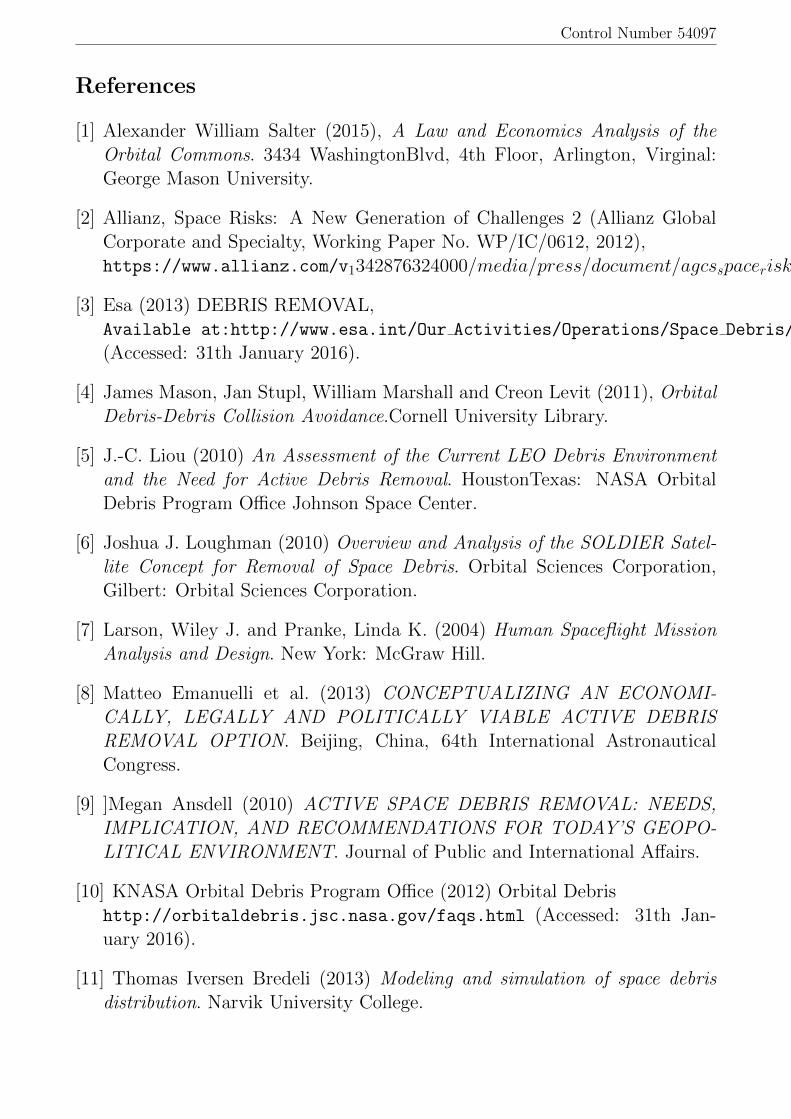
Applying the value and risk models above, it’s obvious that the anticipativevalue could change based on the reduction of the risk growth parameter γ. Itis assumed that the value for γ and d are 0.05 and 6% respectively. Obviouslythe null hypothesis is that there is no risk in this case, the yellow line can beobtained in Figure 1 as the changes of the value over time. If the value of γ is0.05 (the maximum risk parameter), the blue line can be used to instead thechanges. By reducing γ by 0.01 each time, the expected value will lie in thearea between yellow and blue line. For example, the assumed value of γ is 0.04and this value yields red line as the new anticipative value[6].

In this design reference condition, this figure also can indicate the alterationsin value curve over the lifetime of the notional space substance. Following thegrowth of the risk, the expected value reduces along with time. Moreover, thepresent value of future profits will be discounted for some rate. However, therisk will decline with decreasing amount of the debris, while total value willincrease at this case[1].

5.3 Comment

Since this model doesn’t consider the secondary effects of the space junk, therisk parameter is the same as primary value all the time, which is generatedby the exciting space waste. This model can be improved by considering thesecondary impact of the collision of the debris itself as the new parameter forfurther more precise modelling.

6 Cost Estimation Technique

There are mainly two methods to estimate the cost which is estimated cost permission and estimated cost per kg deorbited.


6.1 Estimated cost per kg deorbited

The estimated cost per kg de-orbited (ECD) is a measure of the cost in the re-lation to the missions capability. ECD will define the cost-effectiveness for theanalysed missions. The Active Debris Removal projects are sometimes accusedto be not efficient[7].

6.2 Estimate Cost per Mission

The estimate cost per mission (ECM) is a measure of the total cost of the mis-sion.

We will mainly focus on the estimate cost per mission (ECM) to estimatethe cost of the system. In the following sections, Advanced Missions CostModel is introduced. AMCM provides a useful method for quick turnaround,rough-order-of-magnitude estimating. The model can be used for estimating thedevelopment and production cost of spacecraft, space transportation systems,aircraft, missiles, ships, and land vehicles[7].

6.3 Advanced Missions Cost Model Brady Kalb

The parameters involved in the models are denoted as belowα = 5.56 x 10−4

β = 0.5941Ξ = 0.6604δ = 80.599ε = 3.8085 x 10−55

ϕ = -0.3553γ = 1.5691% = QuantityM = Dry Mass (lbs)S = SpecificationIOC = Initial Operating CapabilityB = Block NumberD = Difficulty

Table 1 AMCM Variable Descriptions


Variable Description

Q Quantity Number of vehicles to be produced

M Mass Dry mass of the vehicle in pounds, does not include fuel or consumables

S Specification Value that designates type of mission

IOC Initial Operating Capability Systems first year of operation

B Block Number Represents level of design inheritance

D Difficulty Number ranging from -2.5 to 2.5 representing difficulty of production

The formula expression is :

Cost = α%βMΞδsε1

IOC−1900BϕγD (7)

This cost estimation technique can be used to determine the overall cost ofthe project. It was developed at NASA Johnson, and has been used on nearlyevery major NASA project in the last 15 years. The advanced mission modelis driven mainly by the dry mass of the vehicle. The variables involved in theformula is shown in the table above with brief descriptions[7].

6.4 Cost Estimation Results

Subsystem Mass (kg)

Payload 100

Structure 50

Thermal 11

Attitude Control 20

Power 66

Communication 13

Propulsion(dry) 16

Propellant 275

Total 551

From the AMCM model, the estimated total cost is $47 million.

CostPerY ear = A(10F 2 − 20F 3 + 10F 4) +B(10F 3 − 20F 4 + 10F 5) + 5F 4 − 4F 5) (8)

In order for the project to be feasible, the cost in any given year must notexceed the proposed yearly budget. NASA currently having a yearly budget ofapproximately $15 Billion. The cost per year schedule shown above was foundusing a 60% Beta Curve. The equation for the 60% Beta Curve is shown asEq.(8), where A is 0.32, B is 0.68, and F, the time fraction, is the percentageof the project development completed in a given year.


6.5 Comments

Although some portions of the spacecraft have not been included in this costanalysis (storage section, fuel tanks, and propellant costs), these costs are mini-mal, and will not greatly affect the estimated cost. The storage section and fueltanks are essentially cylinders, which can be constructed with great simplicity.While the amount of fuel used in the mission is quite large, fuel is relativelyinexpensive when compared to the development and production costs of thespacecraft.

7 Sensitive Analysis of the profit

In the beginning, it is assumed that the project lasted 5 years. From theoutcome simulated by Matlab, the total benefit is gained. At the same time,according to the AMCM calculator, the total cost is estimated to be 47 millions.Then a sensitive analysis of the profit is performed and three different cases areconsidered. 1. In the optimistic case, if the derived value of the project withoutrisk model is considered, the total benefit of the project is estimated to be 225million dollars. The profit is estimated to be 178 million dollars.2. In the normal case, if the derived value of the project with the risk growthparameter 0.04, the total benefit of the project is estimated to be 180 milliondollars. The profit is estimated to be 133 million dollars.3. In the pessimistic case, if the derived value of the project with the riskgrowth parameter 0.05, the total benefit of the project is estimated to be 180million dollars. The profit is estimated to be 128 million dollars.

The estimations are listed in the following table:

Scenarios Profit (million dollars )

Optimistic 178

Normal 133

Pessimistic 128

To sum up, there exists a commercial opportunity for the private firm even inthe pessimistic case. The estimated profit of the firm is between the interval128-178 million dollars with risk growth parameter from 0 to 0.05. However,many other complex situations are still needed to be considered which can makethe result more accurate.


8 Conclusion

From the simulation results, it is concluded that there exists a viable commer-cial opportunity which will bring about profits of million dollars. Although itseems impractical in the real world at present, this space debris removal tech-nology tends to be viable and profitable in the near future. Going forward,the US government needs to work closely with the commercial sector in thisendeavor, focusing on removing pieces of US debris with the greatest potentialto contribute to future collisions[3]. In the meantime, it may also keep its spacedebris removal system as open and transparent as possible to allow for futureinternational cooperation in this field. According to the United Nations 1967Outer Space Treaty, space-based objects including spent rocket boosters andsatellite fragments, belong to the nation or nations that launched them. Hence,international coordination would be required for any sustained effort to captureand remove debris because many nations have contributed to the problem[9].

Although leadership in space debris removal will entail certain risks, investingearly in preserving the near-Earth space environment is necessary to protect thesatellite technology that is so vital to US military and day-to-day operationsof the global economy. By instituting global space debris removal measures, acritical opportunity exists to mitigate and minimize the potential damage ofspace debris and ensure the sustainable development of the near-Earth spaceenvironment.


References

[1] Alexander William Salter (2015), A Law and Economics Analysis of theOrbital Commons. 3434 WashingtonBlvd, 4th Floor, Arlington, Virginal:George Mason University.

[2] Allianz, Space Risks: A New Generation of Challenges 2 (Allianz GlobalCorporate and Specialty, Working Paper No. WP/IC/0612, 2012),https://www.allianz.com/v1342876324000/media/press/document/agcsspaceriskswhitepaper.pdfl

[3] Esa (2013) DEBRIS REMOVAL,Available at:http://www.esa.int/Our Activities/Operations/Space Debris/Debris removal

(Accessed: 31th January 2016).

[4] James Mason, Jan Stupl, William Marshall and Creon Levit (2011), OrbitalDebris-Debris Collision Avoidance.Cornell University Library.

[5] J.-C. Liou (2010) An Assessment of the Current LEO Debris Environmentand the Need for Active Debris Removal. HoustonTexas: NASA OrbitalDebris Program Office Johnson Space Center.

[6] Joshua J. Loughman (2010) Overview and Analysis of the SOLDIER Satel-lite Concept for Removal of Space Debris. Orbital Sciences Corporation,Gilbert: Orbital Sciences Corporation.

[7] Larson, Wiley J. and Pranke, Linda K. (2004) Human Spaceflight MissionAnalysis and Design. New York: McGraw Hill.

[8] Matteo Emanuelli et al. (2013) CONCEPTUALIZING AN ECONOMI-CALLY, LEGALLY AND POLITICALLY VIABLE ACTIVE DEBRISREMOVAL OPTION. Beijing, China, 64th International AstronauticalCongress.

[9] ]Megan Ansdell (2010) ACTIVE SPACE DEBRIS REMOVAL: NEEDS,IMPLICATION, AND RECOMMENDATIONS FOR TODAY’S GEOPO-LITICAL ENVIRONMENT. Journal of Public and International Affairs.

[10] KNASA Orbital Debris Program Office (2012) Orbital Debrishttp://orbitaldebris.jsc.nasa.gov/faqs.html (Accessed: 31th Jan-uary 2016).

[11] Thomas Iversen Bredeli (2013) Modeling and simulation of space debrisdistribution. Narvik University College.


[12] Debra Werner (2015). NASAs Interest in Removal of Orbital DebrisLimited to Tech Demoshttp://spacenews.com/nasas-interest-in-removal-of-orbital-debris-limited-to-tech-demos/(Accessed:02/01/2016)

[13] KNASA Orbital Debris Program Office (2012) Orbital Debrishttp://orbitaldebris.jsc.nasa.gov/faqs.html (Accessed: 31th Jan-uary 2016

[14] Stephen Messenger (2012) Self-Destructing Janitor Satellite to Clean UpSpacehttp://www.treehugger.com/clean-technology/outer-space-no-one-can-hear-you-clean.html

(Accessed: 1st January 2016).


Appendix

For VaR Model

r1=0.05;r2=0.04;r3=0;% risk model growth parameterd=0.06;% value model discount parameterv=300000000;% commmerial satellite revenuet=0:20;% 20 years with interval 1 yearR1=1-exp(-r1.*t); % risk modelV1=(1-R1).*v.*exp(-d.*t); % value modelR2=1-exp(-r2.*t);V2=(1-R2).*v.*exp(-d.*t);R3=1-exp(-r3.*t);V3=(1-R3).*v.*exp(-d.*t);plot(t,V1,t,V2,t,V3,'LineWidth',4)grid onxlabel('Time[yrs]')ylabel('Present[$]')title('Value Effect on Debris Risk Reduction')legend('Derived Value','Derived Value with Reduced Risk','Derived Value without risk model')

For Cost Estimation Technique

alpha = 5.56 * 10ˆ(-4);beta = 0.5941;xi = 0.6604;delta = 80.599;epsilon = 3.8085 * 10ˆ(-55);Psi = -0.3553;Gamma = 1.5691;Q= input('Input Q please:');M= input('Input M please:');S= input('Input S please:');IOC= input('Input IOC please:');B= input('Input B please:');D= input('Input D please:');Cost = alpha* Qˆbeta*Mˆxi*deltaˆS*epsilonˆ(1/(IOC-1900))*BˆPsi*GammaˆD;disp(Cost)

A = 0.32;B = 0.68;F = input('Input F please:'); % time fractionCostPerYear = A*(10*Fˆ2-20*Fˆ3+10*Fˆ4)+B*(10*Fˆ3-20*Fˆ4+10*Fˆ5)+5*Fˆ4-4*Fˆ5;disp(CostPerYear) % every year's percentage of the whole cost

Documents

2016,Problem B