Embed Size (px)
Citation preview

©2016
Lynne C. Trabachino
ALL RIGHTS RESERVED
THE SIGNIFICANCE OF CONVECTIVE CLOUD MICROPHYSICS FOR
CLIMATE MODEL SIMULATIONS OF RAINFALL IN THE WEST AFRICAN
SAHEL AT SEASONAL TIME SCALES
by
LYNNE C. TRABACHINO
A dissertation submitted to the
Graduate School – New Brunswick
Rutgers, The State University of New Jersey
In partial fulfillment of the requirements
For the degree of
Doctor of Philosophy
Graduate Program in Atmospheric Science
Written under the direction of
Mark A. Miller
And approved by
_____________________________________
_____________________________________
_____________________________________
_____________________________________
_____________________________________
New Brunswick, New Jersey
October, 2016
ii
ABSTRACT OF THE DISSERTATION
The Significance of Convective Cloud Microphysics for Climate Model
Simulations of Rainfall in the West African Sahel at Seasonal Time Scales
by LYNNE C. TRABACHINO
Dissertation Director:
Mark A. Miller
This study uses a non-traditional method to substantiate the underlying influence
of the parameterization of subgrid-scale convective processes on the capability of
the latest generation of global climate models to simulate the seasonal cycle of
rainfall associated with the West African monsoon and establish a direct connection
between the treatment of convective rainfall and overall model performance on
seasonal time scales. To establish the degree to which convective parameterizations
iii
may influence model simulations at seasonal scales more definitively, a single
column of grid-scale output was extract from an emissions scenario experiment for
two coupled models and compared to the observed evolution of rainfall, surface
meteorology, the thermodynamic state of the atmosphere, clouds and radiation,
obtained during 2006 in Niamey, Niger. Overall both models demonstrated a
remarkable capability to comprehensively capture the seasonal cycle of the West
African monsoon in the vicinity of Niamey. However, the results confirm that
deficiencies in subgrid-scale physics can be a significant source of error with regards
to the timing of simulated rainfall at seasonal scales and, in some models dominate
non-local sources of error. Comparison of the performance of each model and their
respective convective parameterizations indicated that the capability to simulate
the seasonal cycle of rainfall in the Sahel with realistic timing appears to be more
sensitive to a realistic representation of convective precipitation microphysics than
to a realistic representation of the organization of convective structures. The
perspective gained from this study sheds a more positive light on the present
capabilities of coupled models to simulate convection in the Sahel and suggests
that resolution of the long-standing disagreement in rainfall projections among

iv
different coupled models may be more within reach than previously advocated by
performance evaluations based on traditional methods.

v
Acknowledgements
I would first like to convey my sincere thanks to my advisor, Dr. Mark Miller, for
his time and support throughout my graduate career. I am deeply appreciative for
his patient guidance during the development and completion of this dissertation,
and dedication to my intellectual growth as a scientist and an educator. Mark has
been a great mentor and friend. Without his unwavering belief in me, I would not
be where I am today. I am also very grateful to my committee members, Dr.
Anthony Broccoli, Dr. Leo Donner, Dr. Anthony Del Genio, and Dr. Ben Lintner,
for their indispensable feedback and encouraging response to my research goals.
To have each of these individuals serve me in this capacity is truly an honor.
The completion of this dissertation would not have been possible without
collaborative effort. I am especially indebted to Dr. Michael Jensen and Tami Toto
of Brookhaven National Laboratory who turned the idea of merging radiometric
retrievals with radiosonde measurements into a reality. I would also like to thank
the past and present members of Mark Miller’s physical meteorology research group
at Rutgers, including Dr. Virendra Ghate, Dr. Allison Collow, Lu Wang, Zhongyu
Kuang, Bryan Raney, Jenny Kafka, and Matthew Drews, for providing useful

vi
suggestions and feedback that contributed to the development of this work, and
for the opportunity to contribute to their projects as well. I would like to
recognize John Kelley, my wonderful supervisor while at Lockheed Martin, who
gave me a great start to my career and encouraged me to pursue graduate work.
I am deeply indebted to my family and friends for supporting me on a
personal level. I would like to thank my parents, John and Carole Trabachino, for
the many personal sacrifices they made so that I could continue to pursue my
education. I would also like to thank my sister and her husband, Christine and
Nick Minerowicz, for always opening their home to me and the countless other
ways they have helped me through the last few years. Finally, I thank two very
special friends, Alysun Folden and Jay Arch, for their emotional support and
encouragement.
vii
Contents Abs t r a c t .............................................................................................................. ii
Acknowledgements ................................................................................................ v
List of Tables ....................................................................................................... xi
List of Illustrations ............................................................................................. xii
Chapter 1: Introduction ....................................................................................... 1
1.1 GCM Performance: Capabilities and Challenges ..................................... 1
1.2 Weak Links in the GCM Development Cycle .......................................... 4
1.3 Rainfall Predictions in the Sahel ............................................................. 7
1.4 Connecting Grid-Scale Performance with Local Sources of Error ............ 8
1.5 Goals and Outline ...................................................................................11
Chapter 2: Data and Methods ............................................................................13
2.1 Observations ...........................................................................................13
2.1.1 The RADAGAST Experiment .............................................................13
2.1.2 AMF-1 Instrumentation and Primary Measurements ..........................14
2.2 Climate Models .......................................................................................18
viii
2.2.1 GISS-E2-R ...........................................................................................19
2.2.2 GFDL-CM3 ..........................................................................................20
2.3 Observations Corresponding to Standard Model Output ........................20
2.3.1 2-D Atmospheric Fields ........................................................................20
2.3.2 Thermodynamic Profiles ......................................................................22
Chapter 3: High Resolution Thermodynamic Profiles for Atmospheric Model
Development ........................................................................................................24
3.1 Methods ......................................................................................................28
3.2 Comparison with radiosondes .....................................................................32
3.3 Model evaluation using combined profiles ..................................................42
3.4 Summary and Conclusions .........................................................................55
Chapter 4: Observations ......................................................................................58
4.1 Background Climatology ............................................................................58
4.2 Overview of Observations from RADAGAST ............................................59
4.2.1 Rainfall ............................................................................................59
4.2.2 Surface Meteorology .............................................................................63
ix
4.2.3 The Thermodynamic Environment ......................................................64
4.2.4 Clouds ..................................................................................................66
4.2.3 The Surface Energy Balance ................................................................67
Chapter 5: Observation and Model Comparison .................................................69
5.1 Seasonal Cycles .......................................................................................72
5.1.1 Rainfall ................................................................................................72
5.1.2 Surface Meteorology .............................................................................73
5.1.3 The Thermodynamic Environment ......................................................74
5.1.4 Clouds ..................................................................................................75
5.1.5 The Surface Energy Balance ................................................................76
5.2 Model Intercomparison ...........................................................................78
5.2.1 Errors in Seasonal Cycles .....................................................................78
5.2.2 Correlations ..........................................................................................80
Chapter 6: Connecting Subgrid-Scale Physics with Grid-Scale Performance ......86
6.1 Discussion ...............................................................................................86
6.2 Conclusions .............................................................................................90

x
Appendix A: Computation of CAPE and CIN .....................................................92
Appendix B: Uncertainty equations for cloud microphysical properties ..............96
Appendix C: Simulated Seasonal Cycles of Rainfall in the Region Surrounding
Niamey .............................................................................................................. 100
References .......................................................................................................... 103
xi
List of Tables
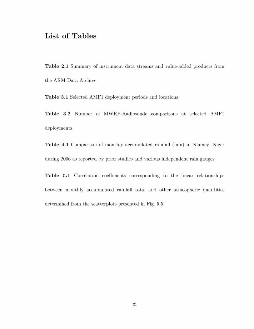
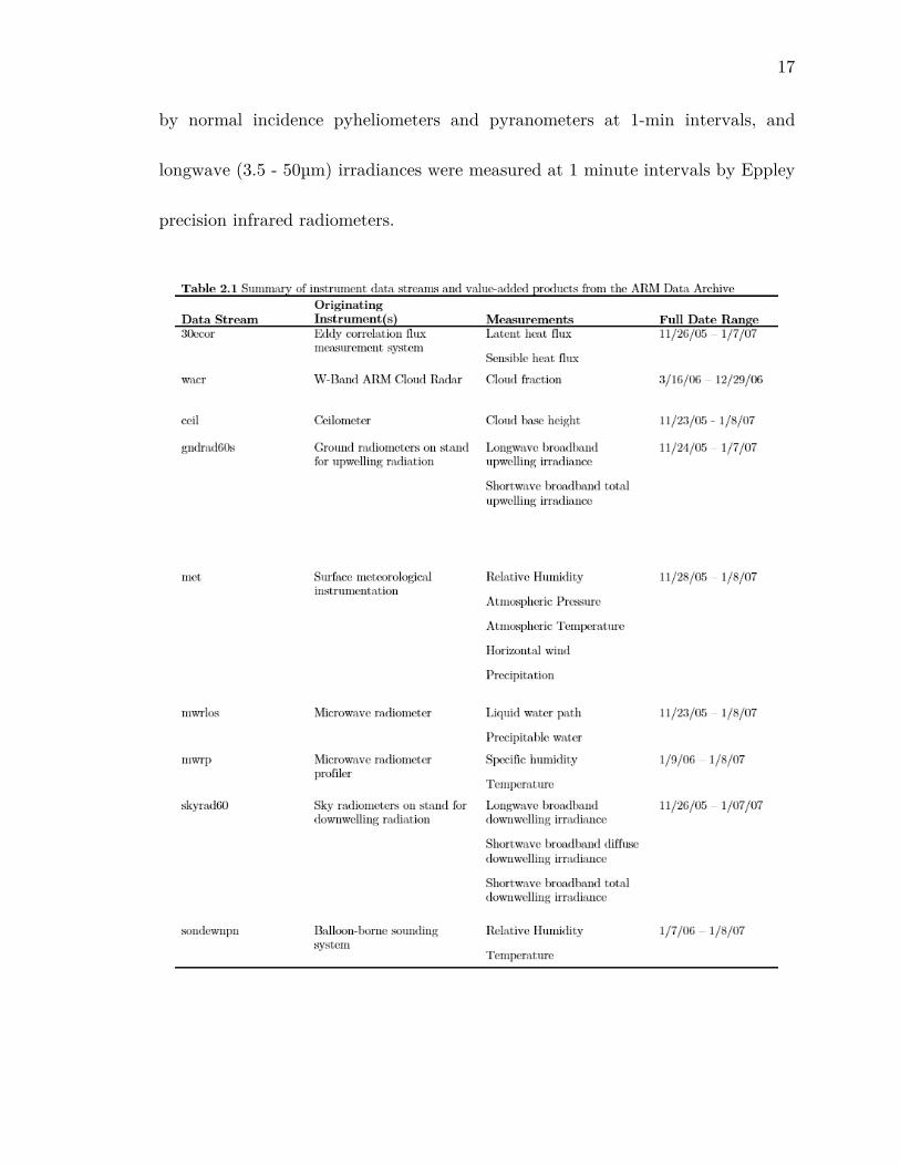
Table 2.1 Summary of instrument data streams and value-added products from
the ARM Data Archive
Table 3.1 Selected AMF1 deployment periods and locations.
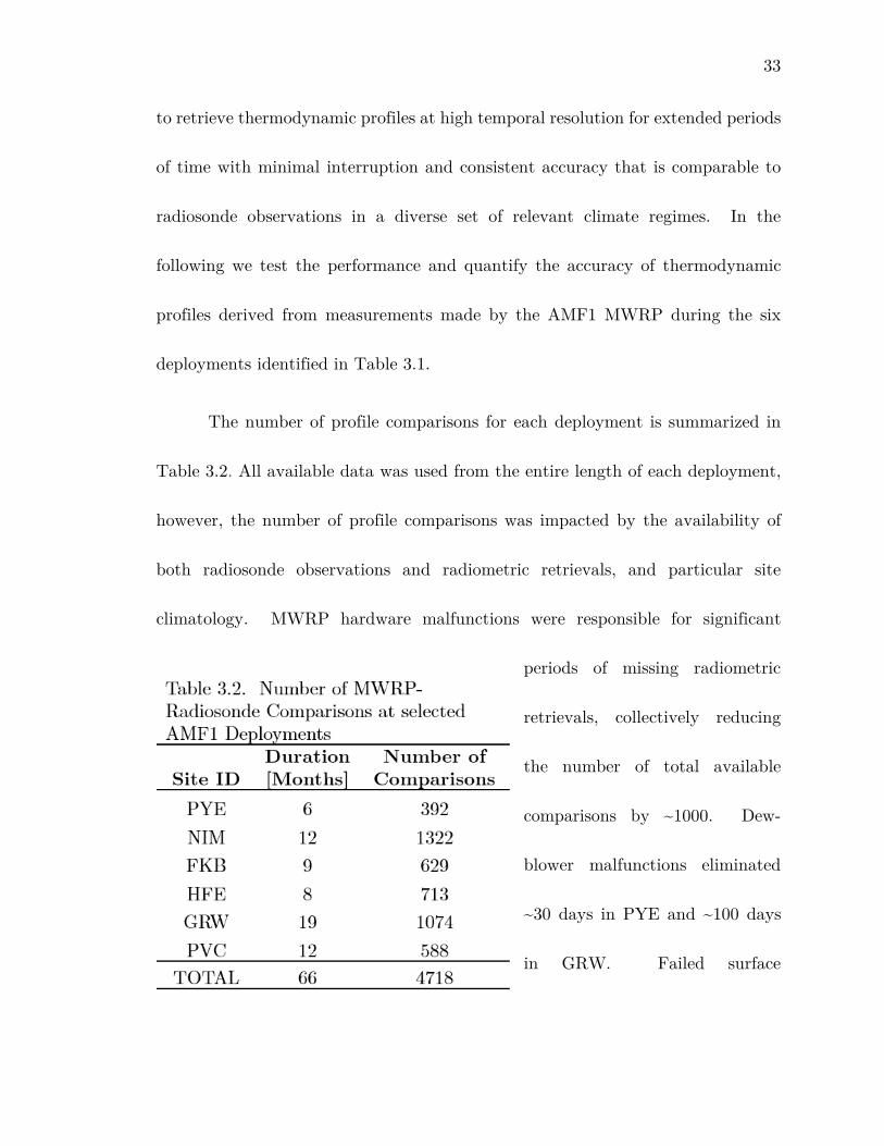
Table 3.2 Number of MWRP-Radiosonde comparisons at selected AMF1
deployments.
Table 4.1 Comparison of monthly accumulated rainfall (mm) in Niamey, Niger
during 2006 as reported by prior studies and various independent rain gauges.
Table 5.1 Correlation coefficients corresponding to the linear relationships
between monthly accumulated rainfall total and other atmospheric quantities
determined from the scatterplots presented in Fig. 5.5.
xii
List of Illustrations
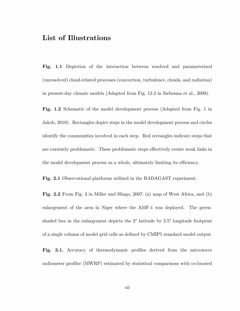
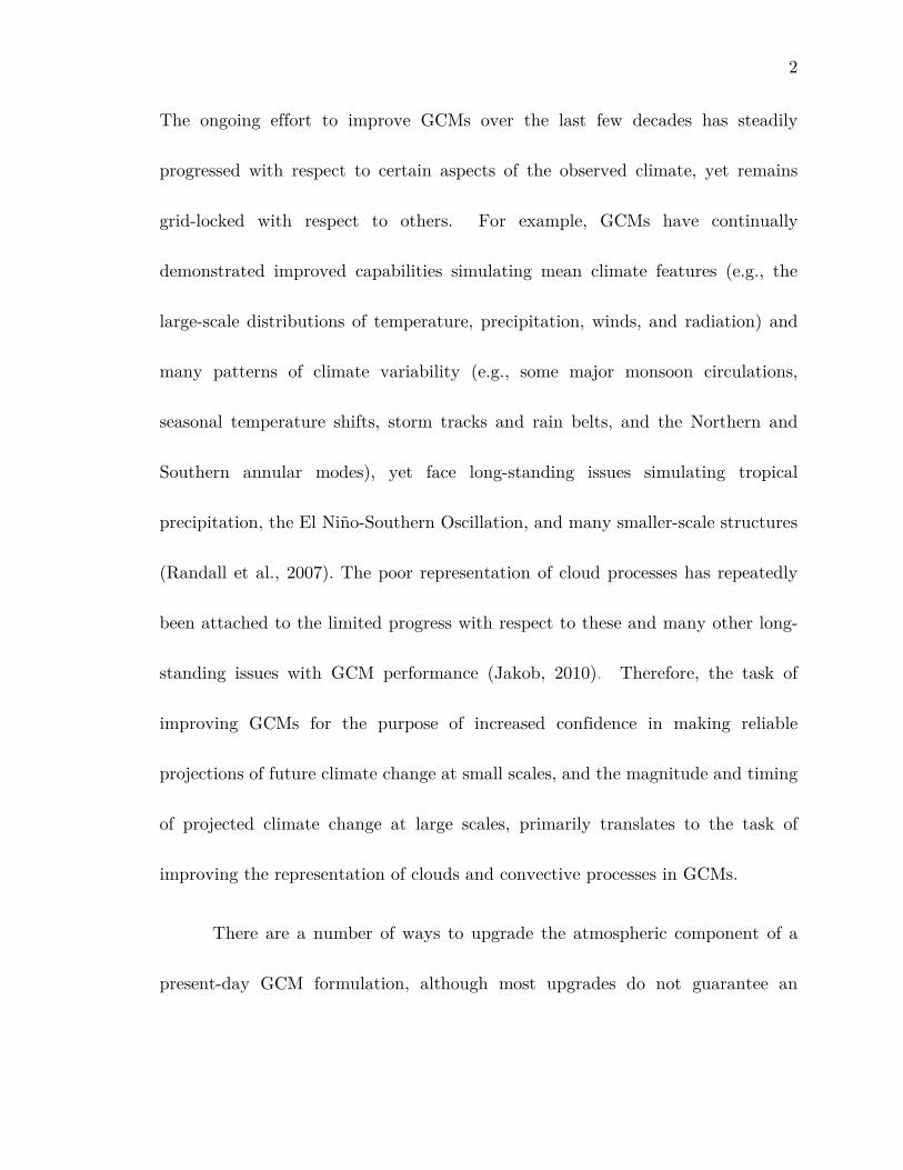
Fig. 1.1 Depiction of the interaction between resolved and parameterized
(unresolved) cloud-related processes (convection, turbulence, clouds, and radiation)
in present-day climate models (Adapted from Fig. 12.2 in Siebesma et al., 2009).
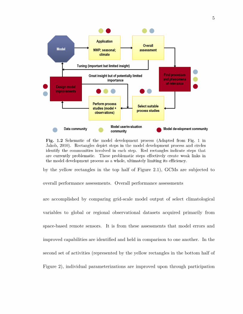
Fig. 1.2 Schematic of the model development process (Adapted from Fig. 1 in
Jakob, 2010). Rectangles depict steps in the model development process and circles
identify the communities involved in each step. Red rectangles indicate steps that
are currently problematic. These problematic steps effectively create weak links in
the model development process as a whole, ultimately limiting its efficiency.
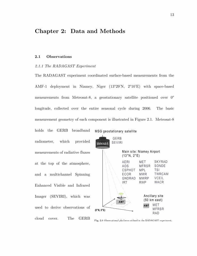
Fig. 2.1 Observational platforms utilized in the RADAGAST experiment.
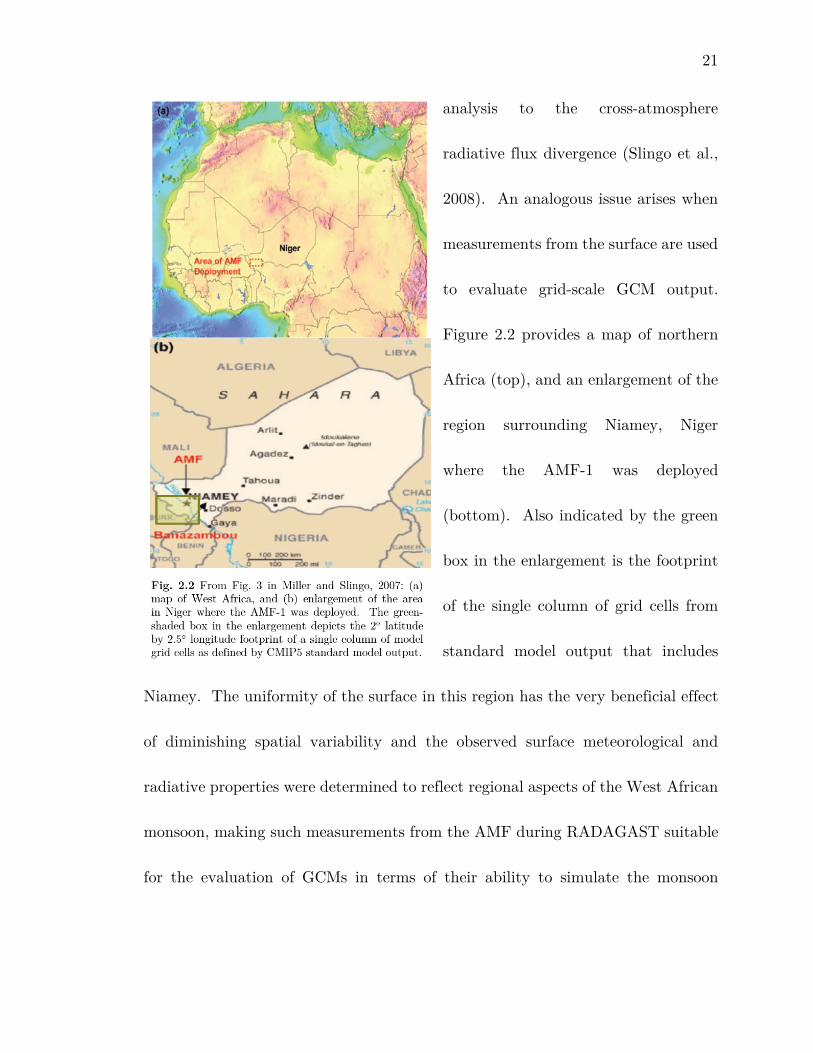
Fig. 2.2 From Fig. 3 in Miller and Slingo, 2007: (a) map of West Africa, and (b)
enlargement of the area in Niger where the AMF-1 was deployed. The green-
shaded box in the enlargement depicts the 2° latitude by 2.5° longitude footprint
of a single column of model grid cells as defined by CMIP5 standard model output.
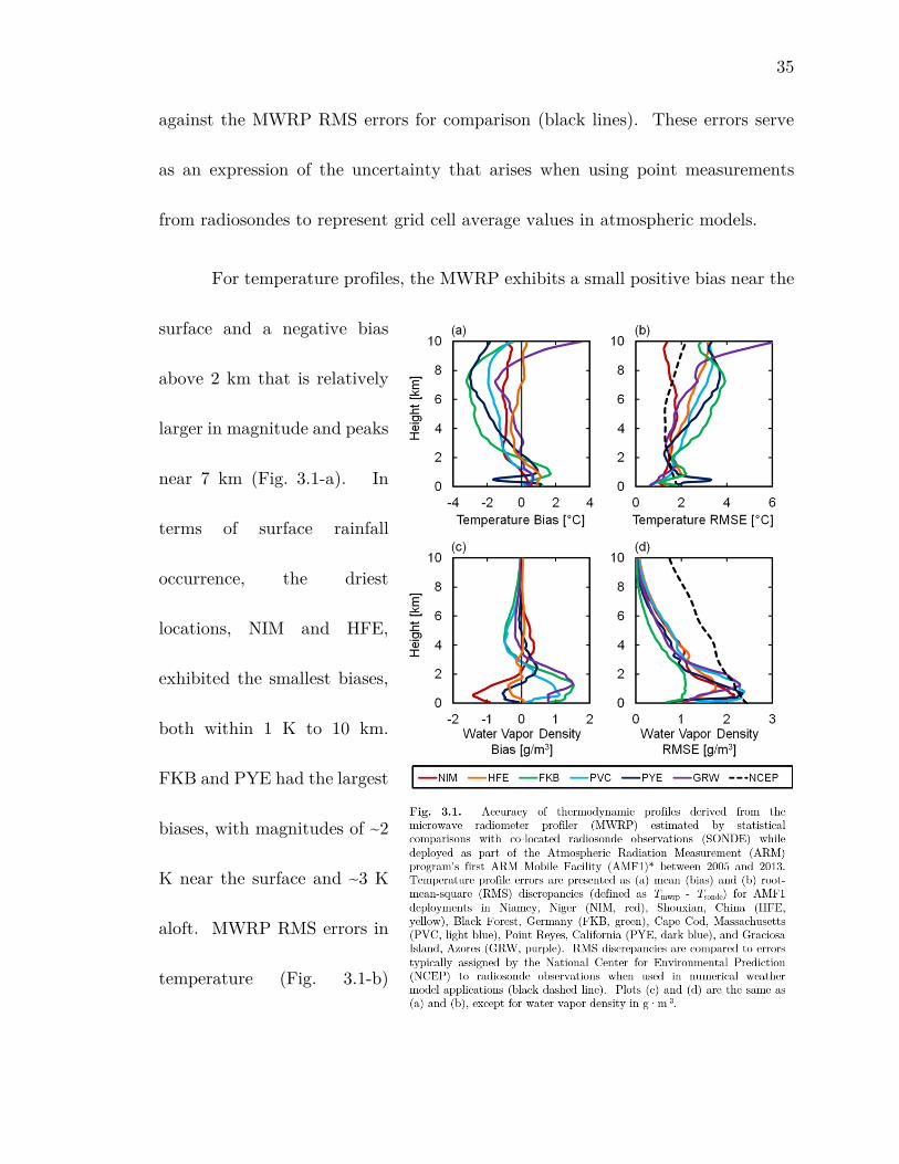
Fig. 3.1. Accuracy of thermodynamic profiles derived from the microwave
radiometer profiler (MWRP) estimated by statistical comparisons with co-located
xiii
radiosonde observations (SONDE) while deployed as part of the Atmospheric
Radiation Measurement (ARM) program's first ARM Mobile Facility (AMF1)
between 2005 and 2013. Temperature profile errors are presented as (a) mean
(bias) and (b) root-mean-square (RMS) discrepancies (defined as Tmwrp - Tsonde) for
AMF1 deployments in Niamey, Niger (NIM, red), Shouxian, China (HFE, yellow),
Black Forest, Germany (FKB, green), Cape Cod, Massachusetts (PVC, light blue),
Point Reyes, California (PYE, dark blue), and Graciosa Island, Azores (GRW,
purple). RMS discrepancies are compared to errors typically assigned by the
National Center for Environmental Prediction (NCEP) to radiosonde observations
when used in numerical weather model applications (black dashed line). Plots (c)
and (d) are the same as (a) and (b), except for water vapor density in g·m-3.
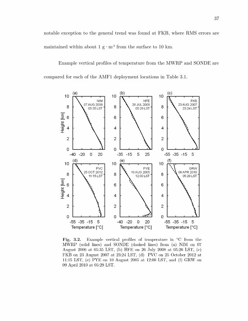
Fig. 3.2. Example vertical profiles of temperature in °C from the MWRP (solid
lines) and SONDE (dashed lines) from (a) NIM on 07 August 2006 at 05:35 LST,
(b) HFE on 26 July 2008 at 05:26 LST, (c) FKB on 23 August 2007 at 23:24 LST,
(d) PVC on 25 October 2012 at 11:15 LST, (e) PYE on 10 August 2005 at 12:00
LST, and (f) GRW on 09 April 2010 at 05:29 LST.
Fig. 3.3. Same as Fig. 3.2, except for water vapor density in g·m-3.
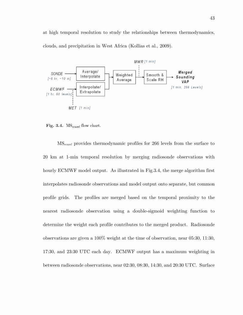
Fig. 3.4. MSecmwf flow chart.
xiv
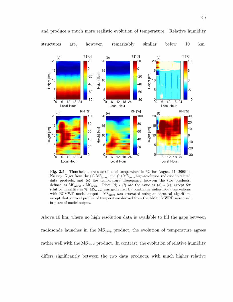
Fig. 3.5. Time-height cross sections of temperature in °C for August 11, 2006 in
Niamey, Niger from the (a) MSecmwf and (b) MSmwrp high-resolution radiosonde-
related data products, and (c) the temperature discrepancy between the two
products, defined as MSecmwf - MSmwrp. Plots (d) - (f) are the same as (a) - (c),
except for relative humidity in %. MSecmwf was generated by combining radiosonde
observations with ECMWF model output. MSmwrp was generated using an identical
algorithm, except that vertical profiles of temperature derived from the AMF1
MWRP were used in place of model output.
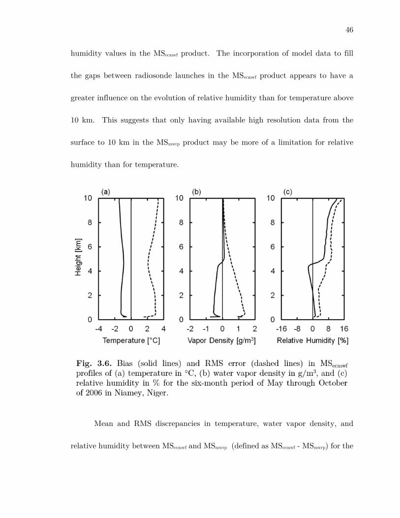
Fig. 3.6. Bias (solid lines) and RMS error (dashed lines) in MSecmwf profiles of (a)
temperature in °C, (b) water vapor density in g/m3, and (c) relative humidity in
% for the six-month period of May through October of 2006 in Niamey, Niger.
Fig. 3.7. Comparison of (a) diurnal and (b) seasonal cycles of CAPE (solid lines)
and CIN (dashed lines) in kJ/kg derived from MSecmwf (red lines) and MSmwrp (black
lines) for the six-month period including May through October of 2006.
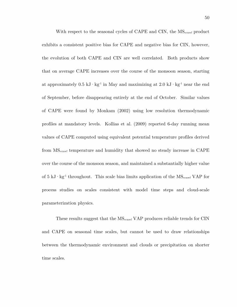
Fig. 3.8. Temperature dependencies of (a) ice water content in g/m3, (b) liquid
water content in g/m3, (c) ice cloud particle effective radius in μm, and (d) liquid
cloud droplet effective radius in μm as defined in the MICROBASE VAP algorithm
assuming a total radar reflectivity factor of -10 dBZ. Error bars represent the
xv
variability resulting from a 3 °C (red) and 1 °C (black) uncertainty in input
temperature profiles.
Fig. 4.1 Time series of monthly-mean (a) accumulated rainfall, (b) near-surface
air temperature, (c) near-surface dew point temperature, (d) near-surface wind
speed and (e) wind direction, (f) surface barometric pressure, (g) near-surface moist
static energy, (h) lifted condensation level (LCL), (i) convective available potential
energy (CAPE), (j) convective inhibition (CIN), (k) cloud area fraction, (l) liquid
water path (LWP), (m) integrated water vapor, (n) surface latent heat flux, (o)
surface sensible heat flux, (p) surface downwelling shortwave (SW) radiation, (q)
surface downwelling SW radiation for clear sky conditions, (r) surface downwelling
longwave (LW) radiation, (s) surface downwelling LW radiation for clear sky
conditions, and (t) surface upwelling LW radiation derived from AMF-1
measurements at the Niamey Airport site during 2006. Months included in the
2006 wet season (May – October) are indicated on each plot by the blue shaded
background.
Fig. 4.2 Comparison of monthly accumulated rainfall (mm) observed during the
2006 monsoon season in Niamey Niger by three independent rain gauges: the AMF-
xvi
1 Present Weather Detector (PWD), the AMF-1 Optical Rain Gauge (ORG), and
an AMMA tipping-bucket rain gauge (TBRG).
Fig. 4.3 Time-height cross sections of monthly-average (a) relative humidity and
(b) temperature generated by combining in-situ measurements from radiosondes
and radiometric retrievals from the microwave radiometer profiler at the AMF-1
site in Niamey, Niger during 2006.
Fig. 5.1 Same as Fig. 4.1 with the envelope of minimum and maximum monthly
quantities simulated by GFDL-CM3 for 2006 – 2015.
Fig. 5.2 Same as Fig. 4.1 with the envelope of minimum and maximum monthly
quantities simulated by GISS-E2-R for 2006 – 2015.
Fig. 5.3 Comparison of time series of monthly-mean errors in the same quantities
as Fig. 4.1 simulated by GFDL-CM3 (red) and GISS-E2-R (purple). Errors are
nonzero for months when the 2006 observed value is not captured within the range
of 2006 – 2010 simulated values for a particular model, and defined as the difference
between the observed 2006 value and the upper or lower boundary of the simulated
decadal envelope.
xvii
Fig. 5.4 Time-height cross sections of errors in monthly-average temperature
profiles simulated by (a) GISS-E2-R and (b) GFDL-CM3, and errors in monthly-
average specific humidity profiles simulated by (c) GISS-E2-R and (d) GFDL-CM3.
Errors are defined as the difference between the observed value at each level during
each month in 2006 and the upper or lower bound of the decadal envelope
simulated by each model during 2006 – 2010.
Fig. 5.5 Monthly-mean values for the quantities in Fig. 3.1 versus monthly-mean
precipitation as observed by the AMF-1 in 2006 (black triangles) and as simulated
during 2006 – 2010 by GISS-E2-R (purple asterisks) and GFDL-CM2 (red open
circles). A linear fit to the monthly-means is indicated by solid lines of
corresponding color. The value of R2 reflecting the amount of variance explained
by each fit is listed in Table 4.2 for each quantity.
Fig. C.1 Envelopes of minimum and maximum monthly-mean rainfall rate
simulated by GISS-E2-R in the grid cells (a) northwest, (b) west, (c) southwest,
(d) north, (f) south, (g) northeast, (h) east, and (i) southeast of (e) the grid cell
containing Niamey, Niger during the period 2006 – 2010 compared to the values
derived from AMF-1 measurements during 2006 in Niamey, Niger.
Fig. C.2 Same as Fig. C.1 except for GFDL-CM3.
1
Chapter 1: Introduction
1.1 GCM Performance: Capabilities and Challenges
The ability to take the appropriate actions today to mitigate the potentially
devastating consequences of anthropogenic influences on Earth’s climate system
hinges on the level of confidence associated with global climate models (GCMs)
used to make projections of future climate change. There is considerable confidence
that GCMs make reliable projections of future climate change at continental scales,
but significantly less confidence at regional scales (Randall et al., 2007; Flato et
al., 2013). GCMs have consistently and univocally predicted climate warming in
response to increased greenhouse gas emissions, although they have yet to converge
with respect to the magnitude and timing of the predicted warming (IPCC, 2013).
These uncertainties present major issues for policy makers. Accordingly, research
in atmospheric science is at present largely focused on assisting model developers
with the key task of improving GCMs.
A major source of confidence in future projections of climate change is the
demonstrated ability of GCMs to simulate observed features of the current climate.
2
The ongoing effort to improve GCMs over the last few decades has steadily
progressed with respect to certain aspects of the observed climate, yet remains
grid-locked with respect to others. For example, GCMs have continually
demonstrated improved capabilities simulating mean climate features (e.g., the
large-scale distributions of temperature, precipitation, winds, and radiation) and
many patterns of climate variability (e.g., some major monsoon circulations,
seasonal temperature shifts, storm tracks and rain belts, and the Northern and
Southern annular modes), yet face long-standing issues simulating tropical
precipitation, the El Niño-Southern Oscillation, and many smaller-scale structures
(Randall et al., 2007). The poor representation of cloud processes has repeatedly
been attached to the limited progress with respect to these and many other long-
standing issues with GCM performance (Jakob, 2010). Therefore, the task of
improving GCMs for the purpose of increased confidence in making reliable
projections of future climate change at small scales, and the magnitude and timing
of projected climate change at large scales, primarily translates to the task of
improving the representation of clouds and convective processes in GCMs.
There are a number of ways to upgrade the atmospheric component of a
present-day GCM formulation, although most upgrades do not guarantee an
3
improved representation of cloud
processes. Upgrades to atmospheric
models typically made while retaining
the current basic architecture of the
formulation (depicted in Figure 1.1)
include: increasing spatial resolution,
increasing complexity through the
addition of previously unrepresented processes; and the improvement of the
physical basis of existing parameterizations. Increasing spatial resolution and
adding complexity to the model formulation by including more processes do not
entirely address the fundamental challenges faced representing a majority of cloud
processes, and in many circumstances do little to improve or even adversely affect
certain aspects of model performance (Illingworth and Bony, 2009). Improving the
physical basis of parameterizations is certainly the most direct route to improving
the representation of cloud processes, but the last few decades have proven this
approach to be difficult and slow to facilitate progress in overall model
performance. A few alternative architectures have been explored to improve the
representation of model clouds, including: global cloud-resolving models (Satoh et
4
al., 2008) and super-parameterizations (Grabowski, 2001; Randall et al., 2003).
Alternative architectures are too computationally demanding for routine
application yet still too coarse to resolve most cloud processes at current operating
resolutions (Siebesma et al., 2009). Over the course of the last decade, a consensus
is forming that the improvement of the physical basis of existing parameterizations
is the most promising way to improve the representation of cloud processes in
GCMs (Stephens, 2005; Illingworth and Bony, 2009; Jakob, 2010).
While there is no shortage of important research questions that would
contribute to the improvement of existing parameterizations in GCMs, it is not the
intention of this work to focus on any single issue in particular. The persistence of
these issues after decades of research suggests that perhaps the responses to the
increasing pressure to improve model clouds can be made more effective by
enhancing the process by which the representation of clouds is improved in GCMs.
1.2 Weak Links in the GCM Development Cycle
The GCM development cycle, schematized in Figure 2, may most basically be
described as an iterative process between two well developed sets of activities that
essentially occur in isolation (Jakob, 2010). In the first set of activities (represented
5
by the yellow rectangles in the top half of Figure 2.1), GCMs are subjected to
overall performance assessments. Overall performance assessments
are accomplished by comparing grid-scale model output of select climatological
variables to global or regional observational datasets acquired primarily from
space-based remote sensors. It is from these assessments that model errors and
improved capabilities are identified and held in comparison to one another. In the
second set of activities (represented by the yellow rectangles in the bottom half of
Figure 2), individual parameterizations are improved upon through participation
6
in offline process studies. Process studies are performed locally, so that detailed
observations of relevant variables for a particular process of interest may be
obtained. These studies serve to improve understanding of the specific physical
mechanisms relevant to a given process and enable the development of
parameterizations that are more physically realistic. The GCM development cycle
as a whole is most efficient when process studies are selected to directly address
the specific aspects of model formulations that are most responsible for overall
performance errors. In practice, problems identified by overall performance
assessments cannot be definitively linked to the underlying deficiencies in the model
formulation. Without definitive guidance about what to fix in the existing
formulation, the development of the next generation of models is driven by other
motivations. However rational these motivations may be, they often do not address
the underlying deficiencies responsible for many of the performance problems
identified in the previous model version (Jakob, 2010). As a result, performance
issues may persist through multiple development cycles, despite the many
improvements incorporated into the formulations with each new generation of
models. The capability of GCMs to adequately simulate Sub-Saharan Sahelian
rainfall is one example of a very critical performance issue that has lacked a
7
connection to specific deficiencies in underlying model physics and has resultantly
persisted through numerous model development cycles over recent decades.
1.3 Rainfall Predictions in the Sahel
There is high confidence that African ecosystems are already being affected by
climate change, and future impacts are expected to be substantial (Niang et al.,
2014). In particular, the Sahel has been identified as a hotspot of climate change
(Diffenbaugh and Giorgi, 2012) where unprecedented temperature changes are
projected to emerge in the later 2030s to early 2040s (Mora et al., 2103). Projected
rainfall change over sub-Saharan Africa in the mid- and late 21st century is,
however, highly uncertain because climate modelers have yet to establish a
consensus with regard to the magnitude and direction of change (Cook and Vizy
2006; Biasutti et al., 2008; Druyan, 2011; Fontaine et al., 2011; Roehrig et al., 2013,
Christensen et al., 2013). Lack of confidence in projected rainfall hinders effective
decision making in efforts to plan and implement adaptation strategies for this
highly vulnerable region.
Intercomparison of coupled GCM simulations indicated no consensus
among the models with regards to the future of the West African Monsoon (WAM)
system (Cook and Vizy, 2006; Roehrig et al.,2013). An evaluation of the capability
8
of models from the fifth phase of the Coupled Model Intercomparison Project
(CMIP5) to simulate the main features of the WAM indicates that the latest
generation of models cannot be relied upon for anticipated climate changes in West
Africa, especially with regard to precipitation (Roehrig et al., 2013). At present,
low confidence in future projections is partially based on the limited success of
CMIP3 and CMIP5 GCMs to simulate the main drivers of the West African
monsoon system, such as the observed correlation between Sahel rainfall and basin-
wide area-averaged SST variability (Christensen et al., 2013) and partially
attributed to non-specific deficiencies in the representation of clouds and
convection in GCMs (Niang et al., 2012). As is the case for many other GCM
performance issues, what the specific deficiencies are and how to identify them
remains unclear.
1.4 Connecting Grid-Scale Performance with Local Sources of Error
By design, traditional model evaluation techniques do not lend their results to
interpretation at scales beyond that which they directly evaluate. Overall
performance assessments (i.e., evaluations of grid-scale climatological mean
quantities) evaluate the spatial distributions of a desired quantity and it relations
to other variables identified as large-scale controls through observations. These

9
studies can therefore identify non-local sources of error in models that don’t
simulate the observed relationship between a given quantity and its known
controls. For example, model inter-comparison studies that evaluate the capability
of models to simulate the known features of the WAM in the present-day climate
provide valuable information with regards to possible non-local sources of error in
the simulation of rainfall in the Sahel, such as SST variability (Niang et al., 2014).
While local sources of error are comingled with non-local sources of error, it is not
possible to isolate their subgrid-scale origins without a comprehensive assessment
of the model physics.
Model physics is typically evaluated by process studies, which evaluate the
physical integrity of parameterization schemes offline, using comprehensive
datasets made available by field studies in a single location. Unfortunately, this
approach is not ideally suited for diagnosing local sources of large-scale performance
issues because the model physics is not being tested in the same environment that
the large-scale performance issues were originally identified (i.e., within the coupled
GCM). While deficient representation of subgrid-scale processes may be diagnosed
based on the nature of physical inconsistencies identified by the evaluation, there
is no direct way to translate the relevance of these errors with respect to overall
10
performance, when the parameterization is operating within the GCM. There is
currently no alternative approach to model evaluation that is focused on bridging
this gap.
Miller et al. (2012) evaluated the seasonal cycle of precipitation and column-
integrated cloud-related quantities simulated by four coupled GCMs by comparing
standard model output sub-sampled from CMIP3 standard model output to
observations from the Radiative Atmospheric Divergence using Atmospheric
Radiation Measurement (ARM) Mobile Facility, Geostationary Earth Radiation
Budget (GERB) data, and African Monsoon Multidisciplinary Analysis (AMMA)
stations (RADAGAST) experiment during 2006 in Niamey Niger. Although the
results of this evaluation were not ultimately applied to diagnose local sources of
error in the simulation of Sahelian rainfall, this study identified a unique window
through which performance evaluations using standard model output could be
interpreted in terms of the convective parameterizations employed by each GCM.
Expanding this technique with the more fully comprehensive set of observations
available from RADAGAST would enable a ‘grid-scale process study’, from which
local sources of error may be diagnosed based on inconsistencies identified by the
evaluation of grid-scale model output.
11
1.5 Goals and Outline
The resolution of long-standing issues with GCM performance, such as those
associated with rainfall in the Sahel, may be greatly benefitted by a better
understanding of local sources of error. This study uses a non-traditional
method to substantiate the underlying influence of the parameterization
of subgrid-scale convective processes on the capability of GCMs to
simulate the seasonal cycle of rainfall associated with the WAM and
establish a direct connection between the treatment of convective
rainfall and overall model performance on seasonal time scales. Standard
model output extracted from CMIP5 emission scenarios of two GCMs will be
evaluated during the present period in terms their capability to capture the
seasonal cycles and inter-relationships between rainfall, near-surface meteorology,
the thermodynamic environment, clouds, and the surface energy balance as
observed during the RADGAST experiment in 2006. This unique approach
effectively applies the diagnostic technique of a process study to seasonal-scale
model output so that convective parameterizations may be evaluated natively,
while operating within their respective GCMs. Not only is this method better
suited to diagnose local sources of error than traditional methods, it’s
12
comprehensiveness offers a new perspective on the capability of GCMs to simulate
the present-day Sahelian climate.
Chapter 2 describes the sources of observations and model output, and the
methodology used for direct comparison. Chapter 4 provides as overview of the
observations from RADAGAST during 2006. In Chapter 5, the performance of
two CMIP5 models is evaluated by direct comparison to the observations presented
in Chapter 4. Chapter 6 provides a summary of major finding and discusses the
limitations of the method applied in this study.
13
Chapter 2: Data and Methods
2.1 Observations
2.1.1 The RADAGAST Experiment
The RADAGAST experiment coordinated surface-based measurements from the
AMF-1 deployment in Niamey, Niger (13°29’N, 2°10’E) with space-based
measurements from Meteosat-8, a geostationary satellite positioned over 0°
longitude, collected over the entire seasonal cycle during 2006. The basic
measurement geometry of each component is illustrated in Figure 2.1. Meteosat-8
holds the GERB broadband
radiometer, which provided
measurements of radiative fluxes
at the top of the atmosphere,
and a multichannel Spinning
Enhanced Visible and Infrared
Imager (SEVIRI), which was
used to derive observations of
cloud cover. The GERB
14
radiometer is described by Harries et al. (2005) and the SEVIRI imager is described
by Schmetz et al. (2002). The AMF-1 provided measurements at the surface
(including the surface energy balance and surface meteorology) and of the column
directly above (including the atmospheric state, cloud properties and aerosol
properties). A full description of the AMF-1 suite of sensors can be found in
Mather and Voyles (2013) or Miller and Slingo (2007).
2.1.2 AMF-1 Instrumentation and Primary Measurements
The AMF-1 Surface Meteorology System (MET) contains a suite of conventional
in-situ sensors that provide measurements of barometric pressure, temperature,
relative humidity, wind speed and wind direction at 1-min resolution. There were
three sources of rainfall measurements at the Niamey Airport site. One-minute
mean precipitation rate was recorded by the AMF-1 optical rain gauge (ORG) and
the AMF-1 Present Weather Detector (PWD). A tipping bucket rain gauge
(TBRG) provided cumulative rainfall totals every 5-minutes.
Vertical profiles of atmospheric temperature and humidity were available
from radiosondes and a 12-channel microwave radiometer profiler (MWRP).
Radiosondes were launched four times daily from the Niamey Airport site,
providing in-situ measurements of atmospheric pressure, temperature, and relative
15
humidity through the extent of the troposphere, sampling every 10 seconds. The
MWRP provides vertical profiles of atmospheric temperature and water vapor
density at 47 levels from the surface to 10 km at 20-second temporal resolution in
all weather conditions except precipitation.
Observations of vertically integrated water vapor (IWV) and the liquid
water path (LWP) in the atmospheric column over the site were derived from
measurements made by the AMF-1 2-channel microwave radiometer (MWR). The
MWR detects atmospheric emissions at 23.8 and 31.4 GHz from water vapor and
liquid water directly overhead every 20 seconds with a field of view of 5.9 degrees.
IWV and LWP are derived by a statistical algorithm that uses monthly linear
regression coefficients determined specifically for Niamey based on a priori data
from radiosonde soundings (Liljegren, 1999). Uncertainties in the LWP and IWV
measurements are ~10 g m-2 and 2%, respectively (Revercomb et al, 2003).
Three active remote sensors were utilized to detect cloud boundaries at the
AMF-1 site: The W-Band ARM Cloud Radar (WACR), the Micropulse Lidar
(MPL), and a laser ceilometer (CEIL). The WACR measures backscatter from
signals emitted every 6 seconds at 95 GHz to a range of 18 km with a range
resolution of 42 meters. The MPL emits 532-nm signals every 30 seconds and
16
measures backscatter to 18 km with a range resolution of 30 m. Using a 905-nm
pulse emitted every 15 seconds, the CEIL detects backscatter from up to 7.5 km
with a range resolution of 15 m.
The AMF-1 Eddy correlation flux measurement system (ECOR) provides
observations of surface latent and sensible heat fluxes every half-hour. ECOR
contains two instruments, a fast-response, three-dimensional sonic anemometer,
and an open-path infrared gas analyzer (IRGA). The sonic anemometer measures
three orthogonal wind components and the speed of sound, which is used to derive
atmospheric temperature. The IRGA measures water vapor density. All three
direct measurements are made at a rate of 10 Hz. Half-hourly observations of
latent and sensible heat fluxes are derived from the direct measurements using the
eddy covariance technique. Based on the measurement accuracies of the three
wind components, the speed of sound, and water vapor density, the expected
uncertainties in the latent and sensible heat fluxes are 5% and 6% respectively
(Cook and Pekour, 2008).
Upwelling and downwelling irradiances were observed at the surface by the
Surface Broadband Solar and Infrared Radiation Station (SIRS) (Stoffel, 2005;
Augustine et al., 2000). Shortwave (295 – 3000 nm) and irradiances were measured
17
by normal incidence pyheliometers and pyranometers at 1-min intervals, and
longwave (3.5 - 50µm) irradiances were measured at 1 minute intervals by Eppley
precision infrared radiometers.
18
Table 2.1 summarizes the instrument data streams available from the ARM
data archive that contain the above mentioned measurements that were utilized in
this study.
2.2 Climate Models
This study utilizes standard model output from CMIP5 representative
concentration pathway (RCP) 4.5 to evaluate the present-day capabilities of two
GCMs: National Oceanic and Atmospheric Administration Geophysical Fluid
Dynamics Laboratory Global Coupled Model 3 (GFDL-CM3) and National
Aeronautics and Space Administration Goddard Institute for Space Studies
General Circulation ModelE2 (GISS-E2-R). These two models were specifically
chosen based on the availability of documentation related to the formulation of
each, and the differences in their respective parameterizations of convection. The
formulations of the atmospheric components of GFDL-CM3 and GISS-E2-R are
described in Donner at al., (2011) and Schmidt et al. (2014), respectively.
Information stated here regarding the representation of convective processes was
sourced from the above-mentioned documents and references therein, source code
made available by the developing institutions, and personal communications with
model developers. Although both models take the same fundamental mass-flux
19
approach to simulate convection, the complexity and physical basis with which
various subgrid-scale convective structures and processes are represented in each
model is quite different. A brief description of the formulation of each model as it
pertains to simulated rainfall in the Sahel is given below to highlight some of these
major differences.
2.2.1 GISS-E2-R
Rainfall simulated by GISS-E2-R originates from the moist convection
parameterization and the stratiform cloud parameterization. Moist convection is
represented in a single column of grid cells by two entraining updrafts and multiple
downdrafts. Convective precipitation originates from convective condensate based
on updraft speeds and the assumption of a Marshall-Palmer particle size
distribution. Within a single grid cell, detrained convective condensate is
ultimately transferred to the large-scale cloud routine (a Sundqvist-type prognostic
cloud water scheme.) which produces precipitation only after evaporating all cloud
water until a threshold relative humidity is reached. Further details with regards
to these parameterizations can be found in Del Genio and Yao (1993), Del Genio
et al. (1996), Gregory (2001), Schmidt et al. (2006), Del Genio et al. (2007), and
Kim et al. (2011,2012).
20
2.2.2 GFDL-CM3
In the Sahel, rainfall in GFDL-CM3 originates entirely from the convective
parameterization. In contrast to GISS-E2-R, the convective structures in GFDL-
CM3 are represented with more realism, but microphysical processes associated
with convective rainfall receive limited treatment. Shallow and deep convection are
represented separately. Deep convection is represented by deep updrafts, mesoscale
updrafts, and mesoscale downdrafts. Precipitation from mesoscale updrafts is
determined as exactly one-half of the sum of condensate formed in mesoscale
updrafts and condensate transferred from convective updrafts. Further details on
the convective parameterization can be found in Donner (1993), Donner et al.
(2001) and Wilcox and Donner (2007).
2.3 Observations Corresponding to Standard Model Output
2.3.1 2-D Atmospheric Fields
It was recognized during the RADAGAST experiment that uncertainty arises from
sampling issues associated with bringing together point measurements from the
surface and area-averaged measurements from space to calculate the radiative flux
divergence over Niamey (Settle et al., 2008). This uncertainty was minimized by
analyzing continuous measurements as daily averages and limiting the scope of the
21
analysis to the cross-atmosphere
radiative flux divergence (Slingo et al.,
2008). An analogous issue arises when
measurements from the surface are used
to evaluate grid-scale GCM output.
Figure 2.2 provides a map of northern
Africa (top), and an enlargement of the
region surrounding Niamey, Niger
where the AMF-1 was deployed
(bottom). Also indicated by the green
box in the enlargement is the footprint
of the single column of grid cells from
standard model output that includes
Niamey. The uniformity of the surface in this region has the very beneficial effect
of diminishing spatial variability and the observed surface meteorological and
radiative properties were determined to reflect regional aspects of the West African
monsoon, making such measurements from the AMF during RADAGAST suitable
for the evaluation of GCMs in terms of their ability to simulate the monsoon
22
circulation (Miller et al., 2009). The applicability of column-integrated
measurements of the radiatively active constituents of the atmosphere (i.e., water
vapor, clouds, and aerosols) and measurements of the vertical structure of
cloudiness and the thermodynamic environment within the atmosphere are
relatively less certain (Miller et al., 2012). However, it is promising that daily-
averaged measurements of aerosol optical thickness were found to be highly
correlated between the main site in Niamey and the auxiliary site 50 km away
(Miller et al., 2009) and results that rely on cloud mask data to determine clear
and cloudy conditions showed essentially no sensitivity as to which cloud mask was
used (Slingo et al., 2009). Limitation of the proposed analysis to monthly-averaged
quantities further supports the applicability of column-integrated quantities.
2.3.2 Thermodynamic Profiles
In this study we combine measurements from a ground-based profiling microwave
radiometer and collocated radiosondes to generate atmospheric temperature and
humidity observations that are tailored to the thermodynamic profiling
requirements of atmospheric model development applications. To establish the
suitability of microwave radiometry for such application, the thermodynamic
profiling capability of a 12-channel microwave radiometer was evaluated against
23
collocated radiosonde observations for extended time periods in a variety of
climatological regimes, including continental and marine environments in the sub-
tropics and mid-latitudes. For the purpose of representing a vertical column of
grid cells in an atmospheric model, in each of the climatological regimes studied,
thermodynamic profiles derived from radiometric retrievals were achievable with
an accuracy similar to that of radiosondes. To demonstrate the utility of combined
profiles for model development applications, a high-resolution data product was
generated using radiometric retrievals to fill in the gaps between radiosonde
soundings and applied to evaluate thermodynamic profiles from a similar high-
resolution data product that was generated using model output to fill in the gaps
between radiosonde soundings. A full description of this methodology is given in
Chapter 3.
24
Chapter 3: High Resolution Thermodynamic Profiles for Atmospheric Model Development
Atmospheric temperature and humidity measurements that are used to develop,
evaluate, and initialize the atmospheric community's entire hierarchy of models are
almost exclusively acquired by radiosondes. However, the spatial and temporal
characteristics of radiosonde observations are poorly suited for modeling
applications, which would benefit most from zenith volumetric measurements that
are representative of atmospheric grid cell volumes. Atmospheric models can have
50 to 200 vertical layers and physics time steps on the order of minutes to an hour.
Radiosonde soundings are a series of point measurements, collected over the course
of a couple of hours as the balloon ascends through the atmosphere. Limited by
cost, equipment, and staffing, it is not routinely feasible to launch more than two
radiosondes per day for extended periods of time. Observations that are more
representative of a vertical column of model grid cells may be derived from
measurements made by zenith-pointing ground-based remote sensors, including
25
microwave radiometers, infrared radiometers, and LIDARs. While relatively coarse
vertical resolution does not restrict the utility of these measurements for modeling
applications, vertical range limitations and operability constraints are more
problematic, to varying degrees. With no alternative measurement technique
capable of all-weather thermodynamic profiling throughout the depth of the
atmosphere, radiosondes remain of crucial importance.
Exclusive reliance on radiosondes for observations of thermodynamic profiles
limits the efficiency of the model development process, particularly with respect to
the improvement of the representation of clouds and convection. The lack of
thermodynamic measurements that are directly comparable to model output on
time scales appropriate for cloud and convective processes compounds the difficulty
of effectively diagnosing model deficiencies. Although the use of radiosondes will
be necessary for the foreseeable future, the atmospheric community could benefit
greatly by incorporating remote sensor measurements to more closely achieve the
thermodynamic profiling requirements of modeling applications.
Ground-based microwave radiometry is a well-established technique for
thermodynamic profiling of the troposphere (Hogg et al., 1983; Solheim et al.,
1998a; Westwater 1993; Westwater et al., 2005). Commercially available
26
microwave profilers are capable of long-term, unattended, daytime/nighttime
equivalent operation in all weather conditions except moderate to heavy
precipitation, and may be used to derive near-continuous vertical profiles of
temperature and humidity with vertical resolution on the order of hundreds of
meters from the surface to 10 km. These attributes make ground-based microwave
profilers uniquely appealing for modeling applications, for which high temporal
resolution is desired and moderate vertical resolution is acceptable (Liljegren et al.,
2001).
Capable of observing both non-dramatic and rapidly changing
thermodynamic variations in the lower troposphere (Güldner and Spänkuch, 2001;
Knupp et al., 2009), radiometric profiles can be used to fill in the gaps between
radiosonde launches. Although vertical resolution degrades linearly with height in
the boundary layer and more rapidly above (Cimini et al., 2006; Cadeddu et al.,
2013), evaluations of a 12-channel profiling microwave radiometer conducted in
Lindenberg, Germany (Güldner and Spänkuch, 2001), and in Lamont, Oklahoma,
and Barrow, Alaska (Liljegren et al., 2001) show that thermodynamic profiles
acquired from radiometric retrievals and radiosonde observations are of similar
accuracy when applied to represent the atmospheric volumes defined by weather
27
forecast model grid cells (Ware et al., 2003). Based on these studies, the primary
utilization of radiometric retrievals has been for data assimilation purposes with
the goal of improving short-term forecasts from numerical weather prediction
models.
It has been recognized that measurements from microwave profilers may be
of similar benefit when used to drive single column models and cloud resolving
model simulations during model development field studies (Liljegren et al., 2001).
The Atmospheric Radiation Measurement (ARM) Program has operated a 12-
channel microwave radiometer profiler (MWRP) as part of its first ARM Mobile
Facility (AMF1) since 2005. The AMF1 is a portable atmospheric laboratory that
includes a suite of remote and in situ sensors designed to collect data in under-
sampled climatologically important regions which may be used by the atmospheric
community to evaluate climate and process models (Miller and Slingo, 2007;
Mather and Voyles, 2013). The extensive dataset available from the AMF1
MWRP presents a unique opportunity to investigate the application of radiometric
retrievals to atmospheric model evaluations.
In this study we present a practical method for obtaining adaptable, high-
resolution thermodynamic profiles that are suitable for application in atmospheric
28
model evaluations by combining measurements from a ground-based profiling
microwave radiometer with co-located radiosonde observations. First, to establish
the use of microwave radiometry for this purpose, data are used from six AMF1
deployments to show that accurate radiometric retrievals are attainable in climate
regimes most relevant to atmospheric model development. We then use combined
radiometric retrievals and radiosonde observations from a single AMF1 deployment
to evaluate a model-based radiosonde-related data product to demonstrate the
advantages of adequate high-resolution thermodynamic profiles for atmospheric
model development.
3.1 Methods
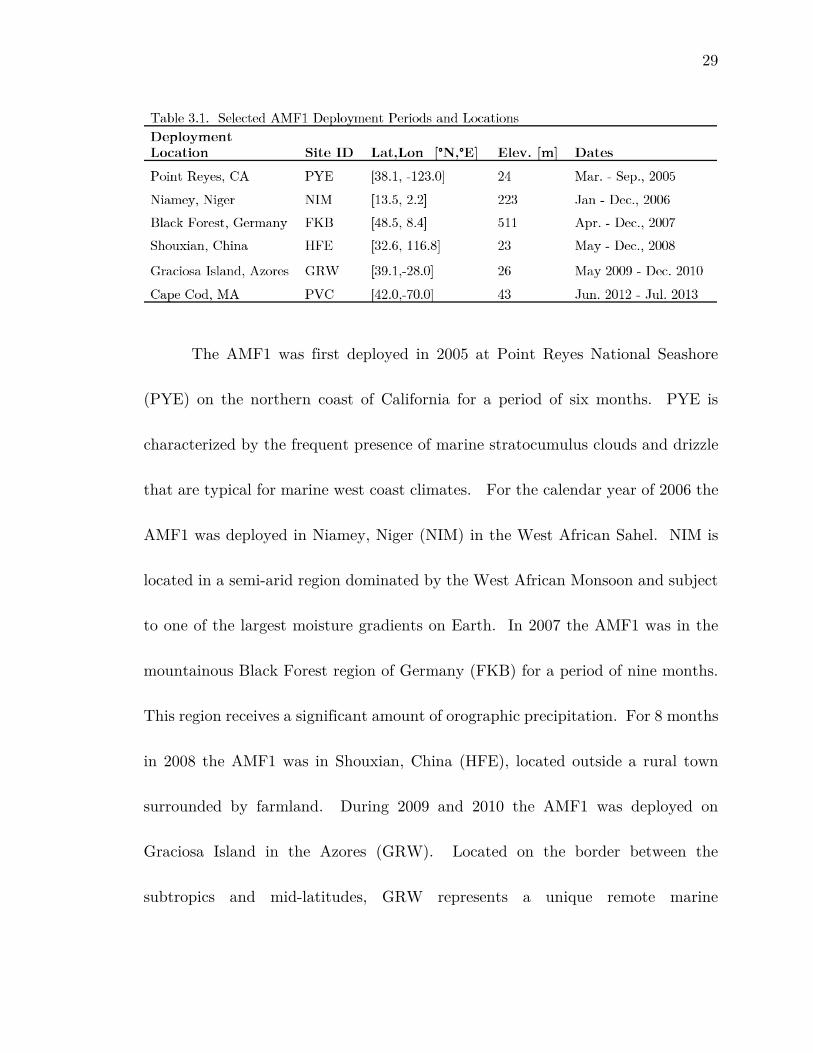
This study utilizes data from the six AMF1 deployment locations summarized in
Table 3.1. The deployments varied in duration from six to 19 months, collectively
providing 66 months of data between 2005 and 2013. Clear and cloudy conditions
in polluted and clean air masses are represented in a diverse set of climatologies
from under-sampled regions throughout the Northern Hemisphere.
29
The AMF1 was first deployed in 2005 at Point Reyes National Seashore
(PYE) on the northern coast of California for a period of six months. PYE is
characterized by the frequent presence of marine stratocumulus clouds and drizzle
that are typical for marine west coast climates. For the calendar year of 2006 the
AMF1 was deployed in Niamey, Niger (NIM) in the West African Sahel. NIM is
located in a semi-arid region dominated by the West African Monsoon and subject
to one of the largest moisture gradients on Earth. In 2007 the AMF1 was in the
mountainous Black Forest region of Germany (FKB) for a period of nine months.
This region receives a significant amount of orographic precipitation. For 8 months
in 2008 the AMF1 was in Shouxian, China (HFE), located outside a rural town
surrounded by farmland. During 2009 and 2010 the AMF1 was deployed on
Graciosa Island in the Azores (GRW). Located on the border between the
subtropics and mid-latitudes, GRW represents a unique remote marine
30
environment. For a period of 12 months during 2012 and 2013 the AMF1 was
deployed in Cape Cod, Massachusetts (PVC).
The AMF1 deployment history provides an ideal dataset for the purposes
of this study. NIM, PYE, and GRW are located in regions with environmental
conditions that present challenges for the operation of remote sensors, and
climatologies that are critical to the development of atmospheric models. The
characterization of the capabilities of profiling microwave radiometers in these
three locations is crucial for establishing the utility of the sensor for atmospheric
model evaluation. The mid-latitude deployments in HFE, FKB, and PVC
represent climatologies where profiling radiometers have been most frequently used,
and therefore serve as a good comparison of the AMF1 MWRP performance
capabilities to that of other studies.
The AMF1 MWRP, Radiometrics Corp. TP/WVP-3000, uses a tunable
frequency synthesizer in the receiver to sequentially measure atmospheric radiance
[W·m-2·sr-1·μm-1] expressed as brightness temperatures [K] at 5 K-Band and 7
V-Band frequencies between 20 and 60 GHz (Solheim et al., 1998a). In this
frequency range, atmospheric emission is dominated by water vapor, atmospheric
oxygen, and cloud liquid water. The K-Band (water vapor sensing) frequencies
31
(22.035, 22.235, 23.835, 26.235, 30.0) and V-Band (temperature sensing)
frequencies (51.25, 52.28, 53.85, 54.94, 56.66, 57.29, and 58.8 GHz) were selected
based on eigenvalue analysis (Solheim et al., 1998b). The calibration of the water
vapor channels is monitored monthly and updated when necessary using the
tipping curve calibration method (Liljegren, 2000; Han and Westwater, 2003).
Temperature sensing channels are calibrated every three to four months with liquid
nitrogen (LN2). The radiometric accuracy of observed brightness temperatures is
0.5 K, although it can be 1 - 2 K in the transparent oxygen channels where the
LN2 calibration is less accurate (Cadeddu et al., 2013). Measurement is impeded
when liquid water on the antenna radome results in artificially high brightness
temperatures. A blower system is used to minimize the accumulation of liquid
water on the radome and a rain sensor provides a flag for potentially contaminated
data. Additional sources of error include artificially high brightness temperature
measurements resulting from observations in directions that are within 15° of the
solar zenith angle and "spikes" caused by radio frequency interference.
Vertical profiles of temperature and humidity are derived from brightness
temperature measurements using a statistical inversion method that is based on
historical radiosonde data specific to each deployment location and a radiative
32
transfer model. The microwave radiative transfer model (Schroeder and
Westwater, 1991) uses the Rosenkranz (1998) absorption model for oxygen and
water vapor, modified for a narrower half-width of the 22 GHz water vapor line
(Liljegren et al., 2005, Garnache and Fisher, 2003) and for the MT-CKD water
vapor continuum (Mlawer et al., 2003). Due to the exponential nature of the
weighting functions in the retrieval algorithm (Askne and Westwater, 1986),
vertical resolution of retrieved profiles based strictly on information provided by
the brightness temperature measurements is relatively coarse: 100 m (500 m) for
temperature (water vapor density) achieved within the first kilometer, and
degrades rapidly above (Cadeddu et al., 2013). However, the fine vertical
resolution contributed by historical radiosonde data allows for thermodynamic
profiles to be provided approximately every 20 seconds for 47 vertical layers from
the surface to 10 km, with 100-m resolution from the surface to 1 km and 250-m
resolution from 1 to 10 km.
3.2 Comparison with radiosondes
Utility for profiling radiometers in atmospheric modeling evaluation is
founded upon the suitability of radiometric retrievals for combination with
radiosonde observations. This suitability specifically translates to the capability
33
to retrieve thermodynamic profiles at high temporal resolution for extended periods
of time with minimal interruption and consistent accuracy that is comparable to
radiosonde observations in a diverse set of relevant climate regimes. In the
following we test the performance and quantify the accuracy of thermodynamic
profiles derived from measurements made by the AMF1 MWRP during the six
deployments identified in Table 3.1.
The number of profile comparisons for each deployment is summarized in
Table 3.2. All available data was used from the entire length of each deployment,
however, the number of profile comparisons was impacted by the availability of
both radiosonde observations and radiometric retrievals, and particular site
climatology. MWRP hardware malfunctions were responsible for significant
periods of missing radiometric
retrievals, collectively reducing
the number of total available
comparisons by ~1000. Dew-
blower malfunctions eliminated
~30 days in PYE and ~100 days
in GRW. Failed surface
34
meteorology sensors eliminated ~60 additional days in GRW. Especially humid
and/or precipitating conditions further reduced the number of available
comparisons at each site to varying degrees. Systematic filtering for these
conditions accounted for the loss of 1 % of available comparisons in NIM, 5 % in
HFE, 16% in PVC and FKB, and 20% in PYE and GRW.
Vertical profiles of temperature and humidity derived from measurements
made by the AMF1 MWRP were evaluated against co-located SONDE
observations. For each profile comparison, SONDE observations were linearly
interpolated to match the vertical resolution of the MWRP, and the first available
single radiometric retrieval within a half-hour of the SONDE launch time was
selected. Statistics of the discrepancies between the MWRP and SONDE (defined
as MWRP - SONDE) observations approximate the accuracy of radiometric
retrievals at each deployment location.
The mean discrepancies (biases) and root-mean-square discrepancies (RMS
errors) between the MWRP and SONDE are presented in Fig. A1 for each AMF1
deployment. Radiosonde errors typically assigned by the National Centers for
Environmental Prediction (NCEP) when assimilating radiosonde observations into
numerical weather models (www.emc.ncep.noaa.gov/gmb/bkistler) are plotted
35
against the MWRP RMS errors for comparison (black lines). These errors serve
as an expression of the uncertainty that arises when using point measurements
from radiosondes to represent grid cell average values in atmospheric models.
For temperature profiles, the MWRP exhibits a small positive bias near the
surface and a negative bias
above 2 km that is relatively
larger in magnitude and peaks
near 7 km (Fig. 3.1-a). In
terms of surface rainfall
occurrence, the driest
locations, NIM and HFE,
exhibited the smallest biases,
both within 1 K to 10 km.
FKB and PYE had the largest
biases, with magnitudes of ~2
K near the surface and ~3 K
aloft. MWRP RMS errors in
temperature (Fig. 3.1-b)
36
range between 1 and 2 K from the surface to approximately 4 km and degrade to
a maximum value between 1.5 and 4 K at about 7 km. Some notable exceptions
to the general trend were found at NIM, PYE, and GRW. For NIM, RMS errors
did not degrade to a maximum value near 7 km, but were maintained within 2 K
throughout the profile. RMS errors at PYE follow a trend similar to that of the
other sites except near a height of 0.5 km, where RMS errors of about 3 K are
uncharacteristically large. To a height of 6 km, RMS errors at GRW are similar
in magnitude to NIM, but then degrade continuously with height to about 6 K at
10 km.
For water vapor density profiles, the MWRP has a negative bias (Fig. 3.1-
c) near the surface and a positive bias aloft at drier locations (NIM, HFE, and
FKB), while the three wetter locations shown the opposite trend, although all are
within 2 g·m-3. RMS errors in water vapor density were remarkably consistent
among the six locations. Near the surface errors are about 1 g·m-3, then reach a
maximum value that is less than 2.5 g·m-3 before 2 km, and then continuously
decrease with height. For all sites, MWRP RMS errors are roughly equivalent to
or less than radiosonde errors at all sites from the surface to 10 km. The only
37
notable exception to the general trend was found at FKB, where RMS errors are
maintained within about 1 g·m-3 from the surface to 10 km.
Example vertical profiles of temperature from the MWRP and SONDE are
compared for each of the AMF1 deployment locations in Table 3.1.
38
Disagreement between the MWRP (solid lines) and SONDE (dashed lines) profiles
is almost exclusively associated with the presence of temperature inversions. While
weak surface inversions are captured by the MWRP relatively well (Fig. 3.2-a) and
3.2-c), discrepancies arise in proportion to the magnitude of the inversion strength
for all inversions above 0.5 km (Figs. 3.2-a to 3.2-f). This suggests that the range
in temperature RMS errors among the different climatological regimes is primarily
due to the height, strength, and persistence of temperature inversions at each site,
and is consistent with the decreasing vertical resolution of the MWRP and the
RMS temperature errors presented in Fig. 3.1. At PYE, for example, the strong
temperature inversion near 0.5 km (Fig. 3.2-e) was persistent throughout the length
of the deployment and can be directly associated with the peak in temperature
RMS errors for PYE near 0.5 km (Fig. 3.1-b). The discrepancy between the
MWRP and SONDE above 8 km at GRW (Fig. 3.2-f) is not associated with a
temperature inversion, however is a consistent problem given the high temperature
RMS errors found in this portion of the profile at RW (Fig. 3.1-b). This is most
likely the result of an issue with the regression coefficients in the retrieval algorithm
generated from historical radiosonde data, but would need to be investigated.
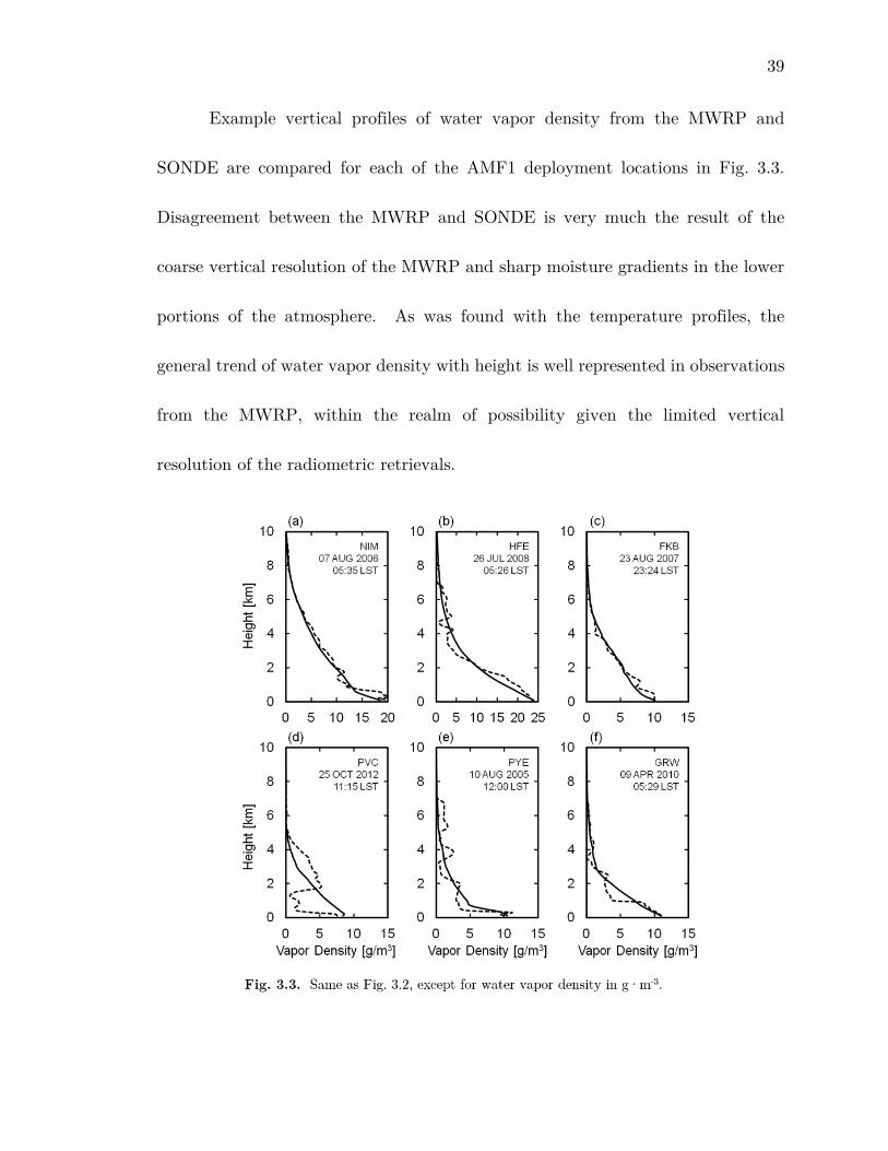
39
Example vertical profiles of water vapor density from the MWRP and
SONDE are compared for each of the AMF1 deployment locations in Fig. 3.3.
Disagreement between the MWRP and SONDE is very much the result of the
coarse vertical resolution of the MWRP and sharp moisture gradients in the lower
portions of the atmosphere. As was found with the temperature profiles, the
general trend of water vapor density with height is well represented in observations
from the MWRP, within the realm of possibility given the limited vertical
resolution of the radiometric retrievals.
40
Our findings establish a unique potential for ground-based microwave
radiometry to provide sufficiently reliable and accurate thermodynamic profiles
with spatial and temporal resolutions that are appropriate for atmospheric
modeling applications. Radiometric retrievals from the MWRP were evaluated
against co-located SONDE observation for extended time periods using data from
six AMF1 deployment locations that represent the marine and continental
environments in the sub-tropics and mid-latitudes. Overall, RMS errors in
temperature ranged 1 - 2 K from the surface to about 4 km and 1 - 4 K to 10 km
and RMS errors in water vapor density were within 2.5 g·m-3 from the surface to
10 km. These errors are similar to the uncertainty that NCEP assigns to point
measurements from radiosondes when they are used to represent grid cell average
values in weather prediction models.
MWRP RMS errors in temperature and humidity at HFE, FKB, and PVC
were equivalent to or slightly larger than reported by Güldner and Spänkuch
(2001), Liljegren et al. (2001), and Cimini et al. (2006) using a similar retrieval
method with an identical radiometer in similar mid-latitude climatologies. Larger
errors may be accounted for by the longer duration (greater than six months) of
each AMF1 deployment in comparison to the much shorter time periods (three to
41
six months) utilized by prior studies. The longer deployment periods in the present
study encompass a broader range of operating conditions within each climate
regime. In addition, calibration of the MWRP was most likely better maintained
during prior studies due to closer monitoring of the instrument. The variability of
RMS errors in temperature among each AMF1 deployment site was also slightly
larger than reported by Westwater et al. (2000) for four different North American
environments, although the current dataset included a more diverse set of
climatologies.
For the purpose of meeting the thermodynamic profiling requirements of
atmospheric modeling applications, the performance of the MWRP at NIM, PYE,
and GRW is generally promising, yet exposes some challenges. MWRP RMS errors
in temperature and humidity at these locations were equal to or smaller than those
from HFE, FKB, and PVC. In NIM, the MWRP operated almost continuously
without interruption for a period of twelve months. However, in the marine
environments of PYE and GRW, although interruptions from rainfall were general
brief, three instances involving hardware malfunctions primarily associated with
the dew blower caused substantial gaps in data availability from periods ranging
for about one month to nearly three months. Close monitoring and mitigation
42
plans for anticipated hardware complications would have to be in place to acquire
long-term continuous datasets in marine environments.
Having demonstrated the profiling capabilities of the MWRP in a diverse
set of climatologies that are specifically relevant to atmospheric modeling
development, we conclude that thermodynamic profiles derived from measurements
made by the MWRP are best exploited for atmospheric modeling applications when
used in combination with radiosonde soundings.
3.3 Model evaluation using combined profiles
Radiosondes and radiometers have a complementary set of advantages with
respect to modeling applications that enables a uniquely effective synergy between
the two instruments that is readily adaptable to the specific thermodynamic
profiling requirements of model evaluations. To illustrate this potential,
radiometric retrievals and radiosonde observations are used in combination to
validate the Merged Sounding (MERGESONDE) Value-Added Product (VAP)
(Troyan, 2012) (referred to hereafter as MSecmwf), a model-based radiosonde-related
data product. MSecmwf profiles are typically used as input for higher order VAPs,
but have also been used for research applications requiring thermodynamic profiles
43
at high temporal resolution to study the relationships between thermodynamics,
clouds, and precipitation in West Africa (Kollias et al., 2009).
MSecmwf provides thermodynamic profiles for 266 levels from the surface to
20 km at 1-min temporal resolution by merging radiosonde observations with
hourly ECMWF model output. As illustrated in Fig.3.4, the merge algorithm first
interpolates radiosonde observations and model output onto separate, but common
profile grids. The profiles are merged based on the temporal proximity to the
nearest radiosonde observation using a double-sigmoid weighting function to
determine the weight each profile contributes to the merged product. Radiosonde
observations are given a 100% weight at the time of observation, near 05:30, 11:30,
17:30, and 23:30 UTC each day. ECMWF output has a maximum weighting in
between radiosonde observations, near 02:30, 08:30, 14:30, and 20:30 UTC. Surface
44
meteorological instrumentation (MET) and a two-channel microwave radiometer
(MWR) provide 1-min observations that serve as boundary conditions at the
surface and scale the relative humidity profiles, respectively.
To evaluate MSecmwf thermodynamic profiles, a similar MWRP-Merged
Sounding (MSmwrp) data product was created using the same algorithm, but 1-min
radiometric retrievals are used in place of hourly ECMWF output. Boundary
conditions provided by MET and the MWR in MSecmwf were not applied. Above
10 km, where radiometric retrievals are not available, radiosonde observations are
simply interpolated. MSmwrp was generated using observations from the AMF1
deployment in Niamey, Niger during 2006. Thermodynamic profiles have the same
spatial and temporal resolution as MSecmwf.
Time-height cross-sections of temperature and relative humidity from
MSecmwf and MSmwrp for 11 August 2006 are compared in Fig. 3.5. Below 10 km,
there are significant differences in the evolution of temperature throughout the
day. The four vertical streaks in MSecmwf occur at the times when the model output
is weighted most heavily. The model output and SONDE observations are not in
good agreement, and the observed structure is a result of the weighted average
used to merge the two data sources. The MWRP and SONDE agree rather well
45
and produce a much more realistic evolution of temperature. Relative humidity
structures are, however, remarkably similar below 10 km.
Above 10 km, where no high resolution data is available to fill the gaps between
radiosonde launches in the MSmwrp product, the evolution of temperature agrees
rather well with the MSecmwf product. In contrast, the evolution of relative humidity
differs significantly between the two data products, with much higher relative
46
humidity values in the MSecmwf product. The incorporation of model data to fill
the gaps between radiosonde launches in the MSecmwf product appears to have a
greater influence on the evolution of relative humidity than for temperature above
10 km. This suggests that only having available high resolution data from the
surface to 10 km in the MSmwrp product may be more of a limitation for relative
humidity than for temperature.
Mean and RMS discrepancies in temperature, water vapor density, and
relative humidity between MSecmwf and MSmwrp (defined as MSecmwf - MSmwrp) for the
47
2006 monsoon season are shown in Fig. 3.6. MSecmwf exhibits a negative
temperature bias of about 1 K from the surface to 10 km (Fig. A6-a). The RMS
difference is 1.5 K near the surface, and 2-3 K to 10 km. These differences are
larger than the MWRP RMS error determined for the year 2006. For water vapor
density, MSecmwf shows a small negative bias, within -0.5 g m-3, to 5 km, and a slight
positive bias, within 0.2 K from 5 to 10 km (Fig. 3.6-b). RMS differences are
within 1.5 g m-3 from the surface to 10 km, which is roughly equivalent to MWRP
RMS errors for the year 2006. MSecmwf and MSmwrp compare extremely well for
relative humidity from the surface to 5 km, with negligible bias and RMS
differences within 5% (Fig. 3.6-c). Above 5 km, MSecmwf tends to be increasingly
more humid with height, although RMS differences are within 15% to 10 km.
These results are consistent with the differences identified between the two data
products in the August 11, 2006 example from the surface to 10 km.
High-resolution thermodynamic profiles allow for the investigation of
relationships between the thermodynamic environment and other meteorological
phenomena that evolve on short time scales, such as cloud cover, precipitation, and
radiation. For such applications it is common to characterize the thermodynamic
environment in terms of derived quantities, such as convective available potential
48
energy (CAPE) and convective inhibition (CIN). Due to the complex definition of
these quantities, it is not immediately clear how the interpretation of CAPE and
CIN may be influenced by uncertainties in the temperature and humidity profiles
from which they have been derived. In the following analyses, we compare time
series of CAPE and CIN computed using temperature and humidity profiles from
MSecmwf and MSmwrp to determine the implications that uncertainties in temperature
and humidity profiles from MSecmwf may have for the utility of time series of CAPE
and CIN derived from this product.
Vertical profiles of temperature and humidity from MSecmwf and MSmwrp were
used to compute CAPE and CIN for the 2006 monsoon season in Niamey, Niger
using simple, psuedoadiabatic parcel theory, as described in Appendix A.
The diurnal and seasonal cycles of CAPE and CIN for the 2006 wet season
in Niamey, computed from each time series, are compared in Figure 3.7. With
respect to the diurnal cycle, MSmwrp values for CIN and CAPE (black lines) range
from 0.1 to 0.2 kJ·kg-1 and 1.2 to 1.6 kJ·kg-1 respectively. CIN tends to a
maximum around 6:00 local time (LT) and a minimum around 15:00 LT, while
CAPE shows an opposing trend, with a maximum at night and a minimum in the
morning. The diurnal cycles of CAPE and CIN from the MSecmwf data product (red
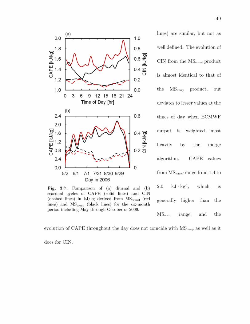
49
lines) are similar, but not as
well defined. The evolution of
CIN from the MSecmwf product
is almost identical to that of
the MSmwrp product, but
deviates to lesser values at the
times of day when ECMWF
output is weighted most
heavily by the merge
algorithm. CAPE values
from MSecmwf range from 1.4 to
2.0 kJ·kg-1, which is
generally higher than the
MSmwrp range, and the
evolution of CAPE throughout the day does not coincide with MSmwrp as well as it
does for CIN.
50
With respect to the seasonal cycles of CAPE and CIN, the MSecmwf product
exhibits a consistent positive bias for CAPE and negative bias for CIN, however,
the evolution of both CAPE and CIN are well correlated. Both products show
that on average CAPE increases over the course of the monsoon season, starting
at approximately 0.5 kJ·kg-1 in May and maximizing at 2.0 kJ·kg-1 near the end
of September, before disappearing entirely at the end of October. Similar values
of CAPE were found by Monkam (2002) using low resolution thermodynamic
profiles at mandatory levels. Kollias et al. (2009) reported 6-day running mean
values of CAPE computed using equivalent potential temperature profiles derived
from MSecmwf temperature and humidity that showed no steady increase in CAPE
over the course of the monsoon season, and maintained a substantially higher value
of 5 kJ·kg-1 throughout. This scale bias limits application of the MSecmwf VAP for
process studies on scales consistent with model time steps and cloud-scale
parameterization physics.
These results suggest that the MSecmwf VAP produces reliable trends for CIN
and CAPE on seasonal time scales, but cannot be used to draw relationships
between the thermodynamic environment and clouds or precipitation on shorter
time scales.
51
Temperature profiles from the MSecmwf VAP serve as a data source for the
Continuous Baseline Microphysical Retrieval (MICROBASE) VAP (Dunn et al.,
2011) to generate vertical profiles of cloud microphysical properties that are in turn
used by higher-order VAPs to generate estimates of atmospheric heating rates.
The MICROBASE VAP employs a mixed-mode phase partitioning scheme and a
set of empirical relationships to derive vertical profiles of liquid water content
(LWC), ice water content (IWC), cloud droplet effective radius (Re) and ice cloud
particle effective radius (Rei) from cloud radar reflectivity and ambient
temperature. In the following analyses, we use the uncertainty in the MSecmwf VAP
temperature profile δT, estimated by statistical comparison with the MSmwrp data
product for the 2006 wet season in Niamey to quantify the uncertainty in the cloud
microphysical properties that MICROBASE supplies to higher-order VAPs.
Uncertainty equations (Appendix B) are formulated using the log-derivative
method and used to demonstrate how the uncertainty propagation resulting from
MSecmwf temperature biases potentially impacts microphysical parameters computed
when MSecmwf temperature profiles are used.
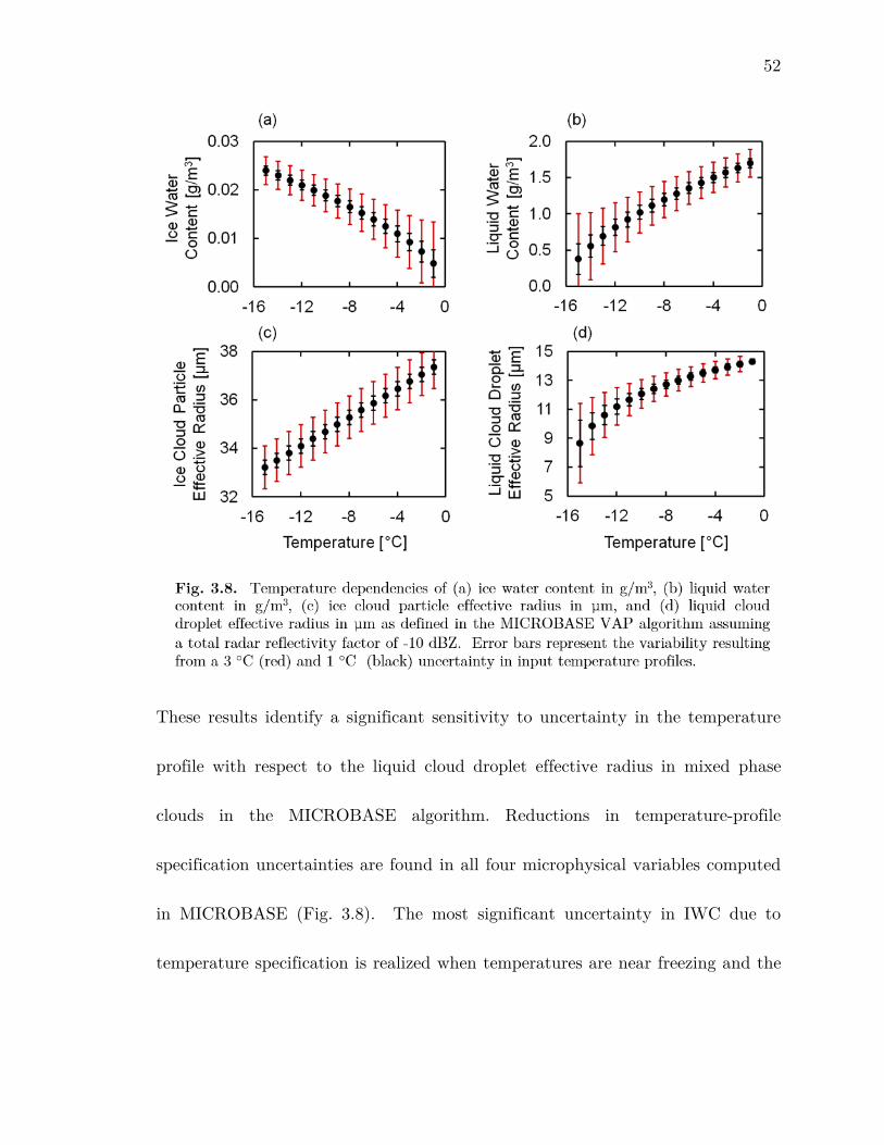
52
These results identify a significant sensitivity to uncertainty in the temperature
profile with respect to the liquid cloud droplet effective radius in mixed phase
clouds in the MICROBASE algorithm. Reductions in temperature-profile
specification uncertainties are found in all four microphysical variables computed
in MICROBASE (Fig. 3.8). The most significant uncertainty in IWC due to
temperature specification is realized when temperatures are near freezing and the

53
uncertainty in Rei is not temperature dependent. Liquid cloud parameters become
progressively more uncertain as the temperatures approach -16 °C, which is the
temperature at which MICROBASE assumes that liquid is no longer present in the
cloud. These uncertainties in the liquid water parameters are a particularly caustic
issue when they are used as inputs to radiation transfer calculations, so any
reduction in the uncertainties is highly desirable.
Evaluating parameterizations in atmospheric models is a challenging
endeavor because observations are often incomplete and incompatible with model
vertical, horizontal, and temporal resolution. A crucial aspect of any model
forecast is the thermodynamic profile because it is integrally related to switches
within the model that toggle various parameterizations on and off. Invoking the
convective parameterization or diagnosing stratiform cloudiness is a function of the
predicted thermodynamic profile, for example, and diagnosing the existence and
phase of clouds within the model column is also a function of this profile. Many
past efforts to evaluate model thermodynamic profiles have relied upon
comparisons between radiosonde profiles collected every few hours and the
predicted thermodynamic profile. But radiosonde thermodynamic profiles are
detailed snapshots, while model calculations in a given grid cell are the result of
54
the convergences and divergences within the models dynamic core; there is an
inherent mismatch between the two profiles. Noting every small fluctuation in the
vertical profile of temperature or water vapor during a radiosonde ascent provides
little that is directly comparable, by itself, with model output. Of more utility is a
continuous, lower resolution thermodynamic profile that mocks model output in
temporal and spatial resolution. The MWRP uses detailed radiation transfer
calculations operating through a mathematical inversion to produce a continuous
estimate of the temperature and water vapor profiles. These profiles often gloss-
over specific details such as sharp inversions in favor of an averaged profile, which
is quite similar to the behavior of the dynamic cores in models, which do not possess
the vertical and temporal resolution to produce anything more.
Beyond the thermodynamic profile as a direct model comparison tool is the
temperature sensitivity of microphysical retrievals that are used to evaluate model
parameterizations. These retrievals operate continuously and require temperature
information to specify the phase of hydrometeors within clouds. Demonstrations
presented herein suggest that a combined MWRP and radiosonde thermodynamic
profile (MSmwrp) provides a superior product relative to a radiosonde and model
derived product (MSecmwf). Despite the 10-km height limitation imposed when using
55
the MWRP measurement between soundings, structures in the lower 10-km are
better resolved when the MWRP is used and it is in these layers where convective
and stratiform cloud parameterizations generally operate. Perhaps most
importantly, the specifications of the MSmwrp product deem it more compatible with
the requirements for evaluation of GCM thermodynamics and process-related
parameterizations.
3.4 Summary and Conclusions
Creating, evaluating, and improving model cloud parameterizations is of critical
importance for virtually all types of atmospheric models, and a particularly urgent
issue for global climate models (GCMs). This study demonstrates that radiosonde
observations and measurements from a profiling microwave radiometer may be
combined to provide thermodynamic profiles that are substantially more
appropriate for atmospheric model evaluations than radiosonde observations alone.
The accuracy of vertical profiles of temperature and humidity derived from
measurements made by the AMF-1 MWRP was estimated by an extensive
statistical comparison with co-located radiosonde observations during the course of
six deployments between 2005 and 2013. To our knowledge, this is the most
extensive and wide ranging comparison to date. It was determined that
56
thermodynamic profiles suitable for combination with radiosonde observations are
attainable from measurements by the MWRP among the diverse set of climate
regimes relevant to atmospheric model development. This result establishes a
unique potential for high-resolution thermodynamic profiles derived from the
combination of radiosondes and radiometers that can be of substantial benefit to
the atmospheric community for use in model evaluations.
Some specific results of this study deserve special mention. Combining
radiosonde and numerical model output to produce a continuous thermodynamic
profile is a useful technique, but it suffers from the need to juxtapose two sources
of information that are somewhat dissimilar and requires the use of techniques to
meld them together even when they exhibit considerable disagreement. The
melding process produces artifacts in the final output product that are clearly
evident when the product is compared to a merged product consisting of two types
of measurements: radiosondes and the MWRP. Artifacts in the radiosonde and
model product propagate into hybrid quantities such as CAPE and CIN, which are
important parameters in cloud parameterizations, and these artifacts may mask
the true relationships between CAPE and CIN and cloud development that need
to be better quantified if they are to be used in cloud parameterizations. Finally,
57
these artifacts introduce unnecessary uncertainty into downstream algorithms that
are sensitive to accurate specification of temperature such as microphysical
retrievals.
High-resolution thermodynamic profiles generated by combining
measurements from a profiling microwave radiometer and radiosonde observations
show potential to enhance the efficiency of the atmospheric model development
process, especially with respect to the improvement of the representation of clouds
and convection. The capability to quantify the uncertainty of model
thermodynamic variables can lead to a better understanding of the sensitivity of
model physics to changes in the thermodynamic profile. It is likely that reductions
in the uncertainty of model thermodynamics can lead to a narrowing of the
variability among different model solutions. A profiling microwave radiometer is
a valuable addition to the suites of remote sensors at research facilities with model
development missions and we recommend that it become a standard instrument at
all sites with this mission.
58
Chapter 4: Observations
4.1 Background Climatology
The lower troposphere in the Sahel region is a transitional zone between the warm,
moist savanna to the south and the hot, dry Sahara Desert to the north. The
transition occurs abruptly along a quasi-stationary Intertropical Front (ITF) and
is experienced at the surface by sharp meridional gradients in temperature and
humidity, and a discontinuity in wind direction. Northeasterly Harmattan winds
allow Saharan air to penetrate the portion of the Sahel north of the ITF, while the
portion south of the ITF is penetrated by relatively cooler, moist air fronm the
tropical Atlantic Ocean. The Sahel is a semi-arid climate zone that experiences
two distinct seasons annually, fundamentally driven by the West African Monsoon
(WAM) circulation. During the boreal winter the ITF is stationed near 10°N,
bringing hot, dry conditions to the Sahel. In spring, the ITF begins a slow
northward migration reaching approximately 20°N in mid-August, during which
time the Sahel receives a majority of its annual rainfall. The ITF then rapidly
retreats southward, and conditions in the Sahel are once again dry by November.
59
At approximately 13.5°N and 2°E, Niamey, Niger is located near the
southern border of the West African Sahel region. The ITF typically passes
northward of Niamey (using the standard criteria of 15 °C of sustained near-surface
dew point temperatures) during the first dekad in April and passes southward
during the last dekad in October (Lélé and Lamb, 2010). Although the monsoon
season spans a period of six months, Niamey receives a majority of its rainfall
during a core period from later July to early September (Slingo et al., 2007).
4.2 Overview of Observations from RADAGAST
4.2.1 Rainfall
The evolution of monthly accumulated rainfall measured using the AMF-1 PWD
during 2006 is shown in Fig. 3.1(a). Rainfall begins modestly in May, steadily
increases to a maximum in August, before rapidly declining back to dry conditions
in November. Niamey received a total of 386 mm of rain from May through
October of 2006, a majority of which (337 mm) occurred during the peak monsoon
months of July, August, and September. Although the monthly accumulated
rainfall total for August was close to average, below normal monthly accumulations
were experienced in all other wet season months (Lélé and Lamb, 2010).
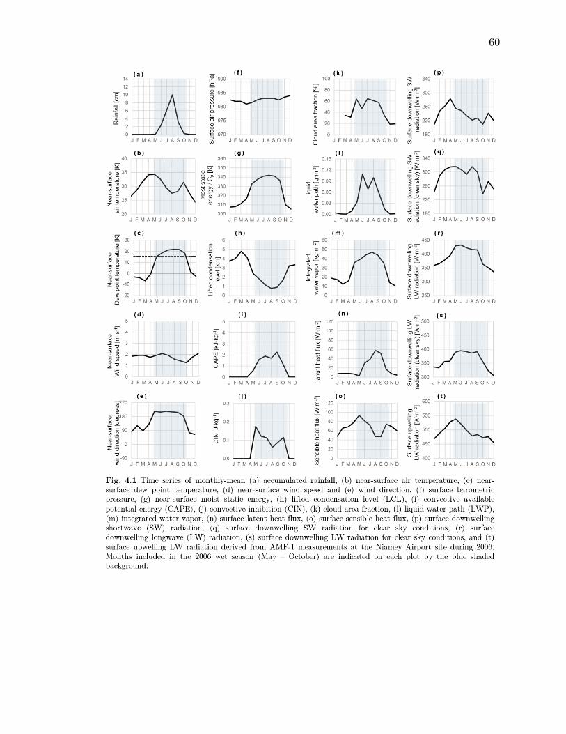
60
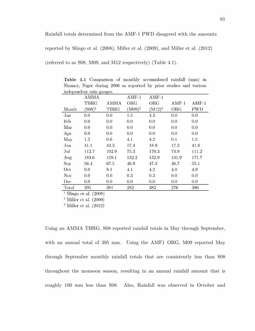
61
Rainfall totals determined from the AMF-1 PWD disagreed with the amounts
reported by Slingo et al. (2008), Miller et al. (2009), and Miller et al. (2012)
(referred to as S08, M09, and M12 respectively) (Table 4.1).
Using an AMMA TBRG, S08 reported rainfall totals in May through September,
with an annual total of 395 mm. Using the AMF1 ORG, M09 reported May
through September monthly rainfall totals that are consistently less than S08
throughout the monsoon season, resulting in an annual rainfall amount that is
roughly 100 mm less than S08. Also, Rainfall was observed in October and
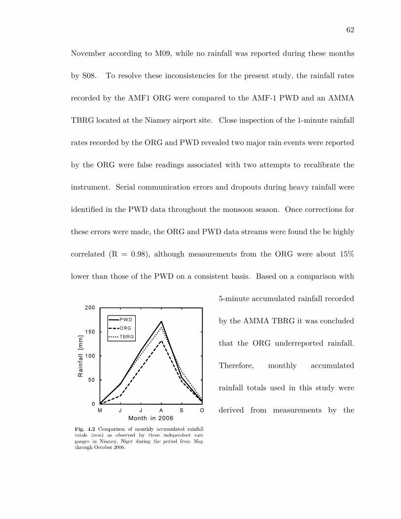
62
November according to M09, while no rainfall was reported during these months
by S08. To resolve these inconsistencies for the present study, the rainfall rates
recorded by the AMF1 ORG were compared to the AMF-1 PWD and an AMMA
TBRG located at the Niamey airport site. Close inspection of the 1-minute rainfall
rates recorded by the ORG and PWD revealed two major rain events were reported
by the ORG were false readings associated with two attempts to recalibrate the
instrument. Serial communication errors and dropouts during heavy rainfall were
identified in the PWD data throughout the monsoon season. Once corrections for
these errors were made, the ORG and PWD data streams were found the be highly
correlated (R = 0.98), although measurements from the ORG were about 15%
lower than those of the PWD on a consistent basis. Based on a comparison with
5-minute accumulated rainfall recorded
by the AMMA TBRG it was concluded
that the ORG underreported rainfall.
Therefore, monthly accumulated
rainfall totals used in this study were
derived from measurements by the
63
PWD. Monthly accumulated rainfall totals for the 2006 season from each
instrument are shown in Fig. 4.2.
4.2.2 Surface Meteorology
Monthly-mean near-surface air temperature and near-surface dew point
temperatures are presented in Fig. 4.1(b) and (c), respectively. Average dew point
temperatures are above 15 °C during May through October, defining the 2006 wet
season. There are two local maxima in near-surface air temperature over the course
of the year, coincident with the beginning and end of the wet season. These results
are consistent with the evolution of daily-mean screen-level temperature and dew
point temperatures reported by Slingo et al. (2008).
Month-mean near surface wind speeds and directions are shown in Fig. 4.1
(d) and (e), respectively. Although wind speeds remain fairly constant throughout
the year, the near-surface wind direction abruptly shifts from northeasterly to
southwesterly at the beginning of the wet season. Southwesterly winds are
maintained throughout the wet season, and abruptly shift back to northeasterly at
the start of the dry season. These results are consistent with evolution of daily-
mean surface wind speed and direction reported by Slingo et al. (2008).
64
Monthly-mean surface air pressure remains fairly constant throughout the
year (Fig. 4.1(f)), with a minimum occurring just before the onset of the monsoon
season and a less pronounced minimum at the end.
Near-surface air temperature and specific humidity measurements from the
AMF-1 MET were used derive surface moist static energy at 1-min resolution (ℎ =
𝐶𝐶𝑝𝑝𝑇𝑇𝑠𝑠 + 𝐿𝐿𝑣𝑣𝑞𝑞𝑠𝑠). Monthly-mean values of moist static energy divided by 𝐶𝐶𝑝𝑝 (Fig.
4.1(g)) abruptly increase at the start of the wet season, then steadily increases
before abruptly dropping back to dry season values at the end of the wet season.
These results are consistent with daily-mean values based on measurements by the
AMF-1 eddy correlation instrument report by Miller et al. (2009).
4.2.3 The Thermodynamic Environment
Monthly-mean vertical profiles of relative humidity and temperature from the
MWRP-MERGESONDE data product described in Chapter 3 are shown in Fig.
4.3(a) and (b), respectively. The presence of the monsoon air mass is evident
during May through October in Fig. 4.3(a), and monthly-average relative humidity
is highest (~70%) through 5 km during the peak season from July to September.
A moderate level of humidity is present in the upper atmosphere for the remained
of the year, with the exception of December, during which time the total
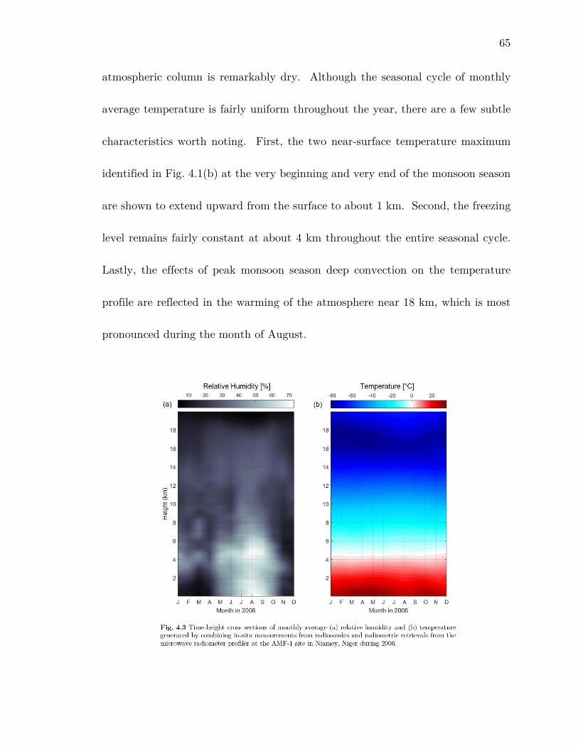
65
atmospheric column is remarkably dry. Although the seasonal cycle of monthly
average temperature is fairly uniform throughout the year, there are a few subtle
characteristics worth noting. First, the two near-surface temperature maximum
identified in Fig. 4.1(b) at the very beginning and very end of the monsoon season
are shown to extend upward from the surface to about 1 km. Second, the freezing
level remains fairly constant at about 4 km throughout the entire seasonal cycle.
Lastly, the effects of peak monsoon season deep convection on the temperature
profile are reflected in the warming of the atmosphere near 18 km, which is most
pronounced during the month of August.
66
Monthly-mean lifted-condensation level (LCL), convective available
potential energy (CAPE), and convective inhibition (CIN) based on simple pseudo-
adiabatic parcel theory (described in Appendix A) are shown in Fig. 4.1 (h), (i),
and (k), respectively. The LCL is highest in March, then drops to half its maximum
value by the start of the wet season, and reaches a minimum in August, coincident
with the rainfall maximum. CAPE is unavailable throughout the dry season, then
abruptly increases with the onset of the monsoon. On average CAPE increases at
a slow, steady rate over the course of the monsoon season, starting at
approximately 0.5 kJ·kg-1 in May and maximizing at 2.0 kJ·kg-1 near the end of
September, before disappearing entirely at the end of October. Similar values of
CAPE were found in this region by Monkam (2002) using low resolution
thermodynamic profiles at mandatory levels. CIN is also not present during the
dry season. Highest values of CIN occur at the onset of the wet season and decrease
steadily to a peak season minimum.
4.2.4 Clouds
Cloud boundaries were determined at 42-meter resolution in the vertical every 6
seconds by combining data from the WACR, MPL, and CEIL as described in
Kollias et al. (2009). Consistent with Miller et al. (2012) cloud area fraction is
67
defined as the fraction of each 1-hour period that clouds were present in the
column. Monthly-mean cloud fractions are variable in the dry season, ranging 20
to 40%, and consistently higher at 60% throughout the length of the wet season
(Fig. 4.1(k)). These values are consistent with the daily-mean cloud fraction
derived from the SEVERI cloud mask (Slingo et al., 2009).
Monthly-mean liquid water path (LWP) and integrated water vapor (IWV)
are shown in Fig. 4.1(l) and (m), respectively. Liquid water is nearly non-existent
in the atmosphere over Niamey during the dry season. The LWP is elevated
throughout the wet season, although the largest values are observed in June, July,
and August of 2006. At the onset of the wet season, total column water vapor
quickly doubles in comparison to its dry season presence, then slowly increases to
a maximum coincident with the peak of the monsoon season, consistent with Miller
et al. (2009).
4.2.3 The Surface Energy Balance
Surface fluxes of latent and sensible heat are shown in Fig. 4.1(n) and (o)
respectively. The latent heat flux (LHF) remains below 10 W·m-2 for the duration
of the dry season months, with a minimum value in May at the beginning of the
wet season. During the wet season the LHF evolves in a manner similar to
68
accumulated monthly rainfall and CAPE, reaching a maximum in August at 60 W
m-2. The SHF evolves as near surface air temperatures, with maxima at the
beginning and end of the wet season.
Surface downward shortwave radiative fluxes for all-sky and clear-sky
conditions are presented in Fig. 4.1(p) and (q), respectively. Clear-sky conditions
were identified using the technique described in Collow et al. (2015). Clear-sky
fluxes peak early in the year, just before cloud cover returns to the Sahel at the
start of the monsoon season then steadily declines until the beginning of the dry
season in November. All-sky fluxes exhibit a similar range of variability although
the decline over the course of the monsoon season is at first slower than that of
the clear-sky fluxes, but more abrupt at the end. Surface downward longwave
radiative fluxes for all-sky and clear-sky conditions are shown in Fig. 4.1(r) and
(s), respectively. These fluxes are largest during the wet season, reflecting the
seasonal cycles of cloud cover and integrated water vapor shown in Fig. 4.1(k) and
(l), respectively.
Surface upward longwave radiative flux is presented in Fig. 4.1(t). This flux
exhibits a maximum value in May that is coincident with the maximum in near
surface air temperature shown in Fig. 4.1(b).
69
Chapter 5: Observation and Model Comparison
GCM performance may be assessed under the expectation that the seasonal cycle
of any given quantity observed during a single year should be contained within the
model-generated envelope of solutions for a decadal period that includes the year
of observation (Miller et al., 2012). In the following, monthly-mean atmospheric
fields for the single column of grid cells over Niamey, Niger was extracted from the
first 10 years (2006 – 2015) of the RCP4.5 emissions scenario dataset for two
CMIP5 coupled GCMs and compared to the observations of rainfall, meteorology,
clouds, and radiation measured during 2006 in Niamey, Niger presented in Chapter
3. Model performance is then assessed in terms of the capability of each model
to: 1) comprehensively capture 2006 monsoon cycle as characterized by the
evolution various atmospheric quantities over the course of the year, 2) reproduce
observed relationships between of such quantities and monthly accumulated
rainfall.
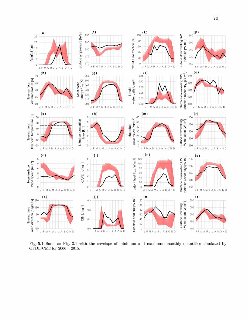
70
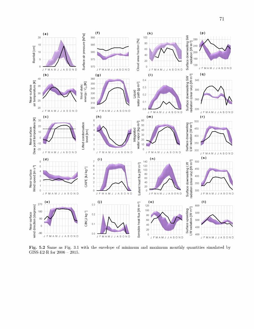
71
72
5.1 Seasonal Cycles
The 2006 – 2015 envelope of seasonal cycles of rainfall, meteorology, the
thermodynamic environment, clouds, and radiation from generated by GFDL-CM3
and GISS-E2-R for the RCP4.5 emissions scenario are compared to the seasonal
cycles observed during 2006 in Niamey in Fig. 5.1 and Fig. 5.2 respectively.
5.1.1 Rainfall
Both models consistently simulate a seasonal rainfall cycle that is centered
on, but extended beyond the observed wet season. GFDL-CM3 generally
overestimates total annual rainfall (64 – 90 cm/year), and the peak rainfall month
tends to occur either too early (as early as May) or too late (as late as October).
The timing and magnitude of the observed annual cycle is better captured by GISS-
E2-R, which simulates peak rainfall in July or August, and produces annual rainfall
total ranging 42 – 67 cm/year. Rainfall that occurs too early (during February
and March) or too late (during November and December) in GISS-E2-R
simulations does not make a significant contribution to the simulated annual
rainfall totals.
Simulated monthly rainfall totals were also extracted for the eight
surrounding grid cells to ensure that spatial displacement was not a significant
73
source of error in the cycles simulated by either model. These results are provided
in Appendix C.
5.1.2 Surface Meteorology
GFDL-CM3 captures the evolution of near-surface air temperature throughout the
year (Fig. 4.1(b)), while GISS-E2-R simulates the basic evolutionary structure
although temperatures are too high during the dry season, and peak one month
earlier than observed (Fig. 5.2(b)). Both models simulate a generally appropriate
range of near-surface dew point temperatures throughout the year (Fig. 5.1(c) &
Fig. 5.2(c)), however both models simulate the onset of the monsoon season too
early, as indicated by the occurrence of dew point temperatures above 15°C. Both
models also fail to simulate the observed increase in dew point temperature over
the course of the wet season.
Both models simulate a seasonal cycle of near-surface wind speeds that was
not evident in the observations (Fig. 5.1(d) & Fig. 5.2(d)). While measurements
during 2006 show little variation in near-surface wind speeds throughout the year,
the models produce high wind speeds during the dry season that slowly decrease
over the course of the wet season. Although this cycle is more pronounced in
GFDL-CM3 than in GISS-E2-R, wind speeds observed during the wet season are
74
captured by the GFDL-CM3 decadal envelope, wind speeds simulated by GISS-
E2-R are consistently higher than observed throughout the year. The observed
shift in wind direction that is characteristic of the monsoon season is captured by
GFDL-CM3 (Fig. 5.1(e)), however wind direction shifts 1 – 2 months earlier in
GISS-E2-R than observed (Fig. 5.2(e)).
Both models exhibit deficiencies simulating the observed surface air
pressure. GFDL-CM3 simulates a seasonal cycle with a minimum in pressure near
the end of the dry season (Fig. 5.1(f)). GISS-E2-R simulates lower than observed
pressure throughout the season but evolves with little variation as observed (Fig.
5.2(f)).
Although both models simulate the observed sharp increase in surface moist
static energy at the start of the wet season, both overestimate the increase and fail
to capture the steady increase in moist static energy over the course of the wet
season (Fig. 5.1(g) and Fig. 5.2(g)).
5.1.3 The Thermodynamic Environment
Simulated seasonal cycles of the LCL, CAPE, and CIN were derived from vertical
profiles output by each model at standard pressure levels using the same algorithm
applied to the observations. Both models capture the magnitude and general
75
evolution of the LCL, although the reduction in LCL at the beginning of the wet
season occurs too early in GISS-E2-R (Fig. 5.2(h)) and too rapidly in GFDL-CM3.
5.1.4 Clouds
Both models capture the seasonal cycle of cloud cover, but with about 10-20% too
much cloud cover during the wet season. Although GFDL-CM3 (Fig. 5.1(k))
produces higher wet season cloud cover amounts (80-100% in June), it captures
the 2006 dry season cloud amount. GISS-E2-R (Fig. 5.2(k)) produces too many
clouds throughout the year, but produces more realistic cloud amounts during the
wet season than GFSL, in comparison to the 2006 observations.
The models each simulate a seasonal cycle for the liquid water path (LWP)
the peaks during the wet season, but these cycles are rather different in terms of
magnitude and evolution. GFSL-CM3 (Fig. 5.1(l)) produces LWP values that
capture the 2006 observations during the dry season, but too low from June
through September. GISS-E2-R (Fig. 5.2(l)) simulates the LWP with values that
are nearly three times larger than observed throughout the year. Despite these
differences, both models capture the 2006 seasonal cycle of total column water
vapor rather well. GFDL-CM3 produces values that closely represent the 2006
observations in all months with the exception of January (Fig. 5.1(m)). GISS-E2-
76
R envelope is slightly higher than the 2006 observation, during the first half of the
year, but still captures the evolution of total column water vapor (Fig. 5.2(m)).
5.1.5 The Surface Energy Balance
The LHF is over estimated during the wet season in both models, however, the
observed evolution of the LHF over the course of the first half of the 2006 wet
season (May – August) is more closely resembled by GISS-E2-R (Fig. 5.2(n)) than
by GFDL-CM3 (Fig. 5.1(n)), which simulates an abrupt increase in the LHF to
peak season values at the beginning of the monsoon season in June. Both models
capture a seasonal cycle for the SHF similar to the 2006 observations, but the
observed May maximum and August-September minimum are each produced
about 2 months early by both models (Fig. 5.1(o) & Fig. 5.2(o)).
GFDL-CM3 captures the evolution and magnitude of the observed 2006
seasonal cycles of surface radiative fluxes extraordinarily well (Fig. 5.1(p) – (t)).
GISS-E2-R produces comparable seasonal evolution but simulates low amounts of
surface downwelling SW radiation for both all-sky and clear-sky conditions, and
simulates large values of surface downwelling longwave radiation for both clear-sky
and all-sky conditions throughout the year (Fig. 5.2 (p) – (t)).
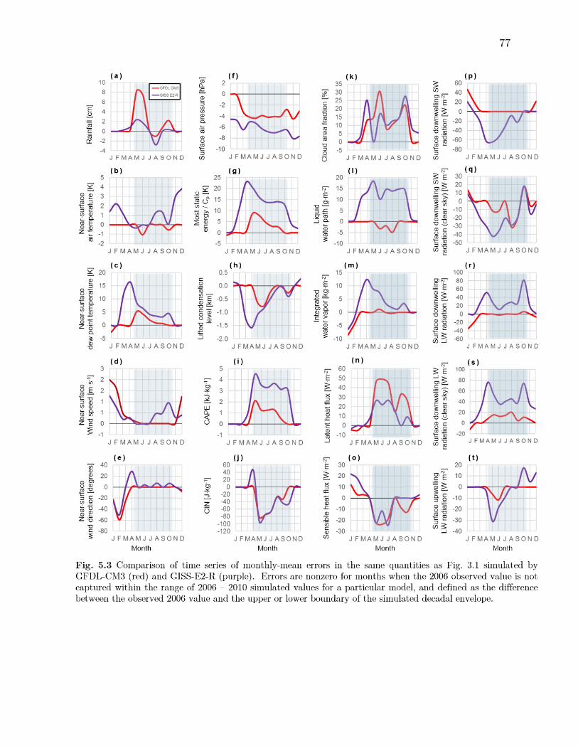
77
78
5.2 Model Intercomparison
5.2.1 Errors in Seasonal Cycles
For any given simulated variable, model error is quantified for each calendar month
as the magnitude of the difference between the value observed during such month
in 2006 and the nearest bound of the decadal envelope simulated by the model.
For months in which a model captures the 2006 seasonal cycle within its decadal
envelope, the model error is defined as zero. Errors corresponding to the decadal
envelopes simulated by GFDL-CM3 and GISS-E2-R are directly compared in Fig.
5.3
With regards to the capability of the models to capture the 2006 monsoon
season, GFDL-CM3 is superior to GISS-E2-R for all evaluated quantities with a
few notable exceptions. The models have roughly equal magnitudes of error with
respect to cloud fraction (Fig. 5.3(k)) and sensible heat flux (Fig. 5.3(o)). GISS-
E2-R has substantially less error than GFDL-CM3 for rainfall (Fig. 5.3(a)) and
latent heat flux (Fig. 5.3(n)). While the model errors frequently differ in terms of
magnitude, they follow remarkably similar trends over the course of the year.
Errors tend to be largest, especially for the GISS-E2-R model, during the transition
79
from the dry season to the wet season in March, April, and May. The larger
magnitudes of error during this time period indicates that the elevated early-season
rainfall in GISS-E2-R is consistent with an early onset of the monsoon reflected by
other simulated quantities (e.g., near surface dew point temperature, wind speeds,
and the LCL).
Following the same method applied above to 2-D atmospheric fields, errors
in simulated monthly-average vertical profiles of temperature and specific humidity
were computed against observed profiles interpolated to the standard pressure
levels available in the model output (Fig. 5.4). For GISS-E2-R, temperature errors
are minimum in the lower atmosphere, but too cool by 2-3 °C between 9 and 12
km during the peak monsoon season. Temperature errors are largest for this model
in the upper atmosphere (but within ±5 °C). Most apparent are warm errors
between 14 and 18 km during January through May, and cool errors near 18 km
during the core of the monsoon season, from June through September. GISS-E2-
R simulates an excess of humidity below 3 km that is most pronounced during
early monsoon season months from April – June with magnitudes near 5 g·kg-1.
GFDL-CM3 presents a rather striking capability to simulate the thermodynamic
environment throughout the entire seasonal cycle. Temperatures are slightly cool

80
(less than 1 °C) for nearly the entire depth of the atmosphere during monsoon
months. Errors in specific humidity for GFDL-CM3 only appear in January (too
dry by about 2 g·kg-1) near 3 km, and in June (too wet by about 2 g·kg-1) at the
surface.
Although GFDL-CM3 captures the seasonal evolution of these variables
with less error than GISS-E2-R, its relatively poor simulation of early-season
rainfall indicates a possible disconnect in the subgrid-scale physics. Whether or not
GFDL-CM3’s simulation of the west African monsoon is less coordinated than that
of GISS-E2-R is further explored in the next section.
5.2.2 Correlations
To further quantify model performance, time series of monthly accumulated rainfall
simulated by each model over the decade from 2006 – 2015 were correlated with
all other quantities individually (Fig. 5.5). Correlation coefficients characterizing
the relationship between rainfall and all other quantities were evaluated against
correlation coefficients determined from the observations in 2006 (Table 5.1).
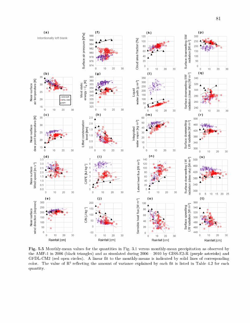
81
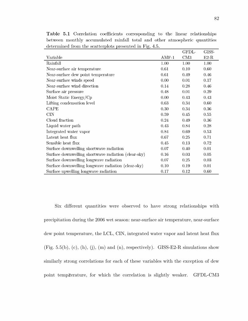
82
Six different quantities were observed to have strong relationships with
precipitation during the 2006 wet season: near-surface air temperature, near-surface
dew point temperature, the LCL, CIN, integrated water vapor and latent heat flux
(Fig. 5.5(b), (c), (h), (j), (m) and (n), respectively). GISS-E2-R simulations show
similarly strong correlations for each of these variables with the exception of dew
point tempzerature, for which the correlation is slightly weaker. GFDL-CM3
83
simulations reproduce a strong correlation between precipitation and integrated
water vapor, but reproduce weak correlations with respect to the near-surface dew
point temperature, LCL, CIN and LHF, and essentially no relationship between
precipitation and near-surface air temperature.
Surface air pressure, CAPE, cloud fraction, LWP, and sensible heat flux
were observed to correlate weakly with precipitation in 2006 (Fig. 5.5(f), (i), (k),
(l), and (o), respectively). GISS-E2-R reproduces similarly weak correlations for
each of these quantities, with the exception of the sensible heat flux, which exhibits
a strong relationship with simulated precipitation. GFDL-CM3 simulations show
weak relationships with respect to cloud fraction and CAPE that are similar to the
observed. However, GFDL-CM3 reproduces a strong correlation with respect to
the LWP, and essentially no correlation with respect to surface air pressure and
the sensible heat flux.
Observations during 2006 revealed little or no relationships between the
seasonal cycle of precipitation and wind speed, wind direction, moist static energy,
or any of the surface radiative fluxes (Fig. 5.5(d), (e), (g), (p)-(t), respectively.)
GISS-E2-R simulations show similarly weak correlations for near-surface wind
speed, downward shortwave radiation at the surface for all-sky and clear-sky, and
84
downward longwave radiation at the surface. Wind direction and moist static
energy exhibit weak correlations in GISS-E2-R simulations, and a uniquely strong
correlation is shown with respect to upward longwave radiation at the surface.
GFDL-CM3 reproduces the observed weak correlations between precipitation and
wind speed, downward shortwave radiation at the surface for clear-sky conditions,
and upward longwave radiation at the surface. Weak correlations are found with
respect to wind direction, moist static energy, downward shortwave radiation at
the surface (all-sky) and downward longwave radiation at the surface.
On the basis of these results, the originating sources of error with respect to
the simulation of rainfall appear to be unique to each model. Simulations from
GISS-E2-R reproduced relationships between precipitation and nearly all evaluated
quantities that were remarkably similar to those observed during 2006. The fact
that the evolution of rainfall is largely consistent with the evolution of other
atmospheric fields suggests that the treatment of convective rainfall in this model
does not contain deficiencies that significantly influence model performance on
seasonal time scales. The tendency to of this model to simulate the start of the
monsoon season early is then most likely rooted in non-local sources of error.
GFDL-CM3 captures the 2006 seasonal cycles for nearly all evaluated quantities,

85
yet does not reproduce the observed relationships between the evolution of rainfall
and all other quantities. The dominant source of error in this model appears to
come from deficiencies in the treatment of convective rainfall.
86
Chapter 6: Connecting Subgrid-Scale Physics with Grid-Scale Performance
6.1 Discussion
The persistent lack of agreement in projections of rainfall in the Sahel among
different GCMs has been generally attributed to challenges associated with the
representation of convective processes. To establish the degree to which convective
parameterizations may influence seasonal-scale model output more definitively, a
single column of standard model output was extracted from the CMIP5 dataset for
two GCMs and compared with the observed seasonal evolution of rainfall, surface
meteorology, the thermodynamic state of the atmosphere, clouds and radiation,
obtained during the RADAGAST experiment in Niamey, Niger. This approach
enables a unique comprehensive assessment of seasonal rainfall simulations and
provides valuable insight into how the parameterization of convective processes
relate to model performance on seasonal scales that could not be gained from
traditional model evaluations techniques. It was found that local sources of error
87
originating from the representation of subgrid-scale convective processes may
significantly impact simulations of the seasonal cycle of rainfall in some models.
Based on the relative performance of each model in combination with their
respective formulations, a physically-based treatment of convective rainfall may be
critical to successful simulation of rainfall on seasonal time scales.
Some additional findings deserve specific mention. First, both models
demonstrated a remarkable overall capability to simulate the set of variables
representing the seasonal cycles of surface meteorology, the thermodynamic
environment, clouds and radiation that characterize the WAM. A less
comprehensive study that uses JAS rainfall totals as a reflection of the capability
of GCMs to simulate convection may not reach the same conclusion. As
demonstrated by the performance of GFDL-CM3 in this study, low JAS rainfall
may result from errors in timing of peak-season rainfall, not the inability of the
model to simulate a monsoon season. As also demonstrated by GFDL-CM3, errors
in timing may simply be a reflection of the model’s handling of convection
precipitation, and does not speak for its ability to simulate other aspects of
convection. These considerations shed a different light the capability of GCMs to
88
simulate the WAM and allow for the possibility that progress simulating
convection in this region may be understated.
The availability of only a single year of observations in Niamey is a
significant limitation with two major implications for the present study. First, the
observed correlation coefficients that quantify the relationships between rainfall
and all other quantities are less robust than those computed for the simulations,
which were determined from 10 years of data. Second, it is not possible to evaluate
the year-to-year variability in the simulated seasonal cycles, which could have
illuminated additional errors that were otherwise not identified by this study.
These limitations, however, should not overshadow the fact that the RADAGAST
dataset represents a rare wealth of observations that may not be available in the
Sahel again for some time.
The uniformity of the landscape in the Sahel is a major factor that allows
for the comparison of grid-cell average quantities to point observations as done so
in this study. Successful application of this method to other regions with similar
available datasets from other AMF-1 deployments is not immediately obvious.
Additional research would most likely be required to show that monthly-average
observations are comparable to model output in other locations. How applicable
89
the results of the present study are to the rest of the Sahel is unclear. Further
study is required to determine how local and non-local sources of error may vary
in relation to each other within a given region.
Despite the above-mentioned limitations, the analysis defined by the scope
of this study hardly exhausted the utility of the evaluation dataset. Specifically,
further evaluation could have been performed by comparing simulated and
observed relationships between all possible combinations of quantities. Such results
may be useful to study the influence of the models’ formulations of convective
processes other than rainfall on seasonal-scale performance. The results of this
study might also be especially useful for interpretation of the future rainfall
projections for the emissions scenario dataset that was utilized in the present-day
evaluation. GCM capabilities to reproduce the present-day climate are typically
limited to a historical time period that precedes the start of emission scenario
projections. The fact that the simulations used in this study to represent the
present-day climate were extracted from the first decade of data available for
RCP4.5 makes the results of the evaluation slightly more relevant for the
interpretation of future rainfall projections in the Sahel.
90
6.2 Conclusions
This study confirms that deficiencies in subgrid-scale physics can be a significant
source of error in GCM simulations of rainfall at seasonal scales and, in some
models dominate non-local sources of error. While deficiencies in subgrid-scale
physics are unique to each model’s formulation, the capability to simulate the
seasonal cycle of rainfall in the Sahel appears to be more sensitive to a realistic
representation of convective precipitation microphysics than to a realistic
representation of the organization of convective structures. Information
characterizing the nature of errors in rainfall simulations at seasonal scales such as
this can be a valuable supplement to model evaluations performed using traditional
methods and ultimately help expedite the resolution of long-standing issues with
GCM simulations in the Sahel.
Increasing the certainty in GCM projections of rainfall in the Sahel is but
one of many important challenges that model developers continue to be faced with.
Given these challenges, an effort to increase the efficiency of the model development
process is a task of equal importance to development efforts in and of themselves.
Although this study sheds light on the enormity of the task at hand, it also
illuminates a path by which the larger scientific community can contribute to an
91
increased understanding of model performance, given knowledge of how GCMs are
formulated.
The sensitivity of seasonal-scale GCM performance in the Sahel to the
microphysical treatment of convective precipitation in the model’s formulation
provokes further exploration into the mechanisms of communication between the
land surface and the atmosphere in this region. Future work should answer key
questions regarding the relevance of these microphysical communications to the
evolution of rainfall within a given season and how these communications may be
effected in future climate change scenarios. Such knowledge would be invaluable
not only for the Sahel, but for any other region that depends so critically on its
local agriculture.
92
Appendix A: Computation of CAPE and CIN
The following describes the methodology used to approximate CAPE and CIN
based on the ascent of a mixed-layer parcel using simple, psuedoadiabatic pure
parcel theory. The MSecmwf and MSmwrp high-resolution data products provide
temperature Tc in °C, relative humidity, RH in %, and barometric pressure, P in
mb, for 266 levels from the surface (level 0) to a height of 20 km (level 266).
Physical constants used in this formulation were defined as follows: Gas
constant for dry air, Rd = 287.04 J·kg-1·K-1, gas constant for water vapor, Rv =
461.50 J·kg-1·K-1, specific heat of dry air at constant pressure, Cpd = 1005.7 J·kg-
1·K-1, specific heat of water vapor at constant pressure, Cpv = 1875 J·kg-1·K-1,
acceleration due to gravity, g = 9.81 m·s-2. Meteorological variables, including
absolute temperature, potential temperature, virtual temperature, vapor pressure,
and water vapor mixing ratio were computed using the relationships and empirical
formulas of Bolton [1980].
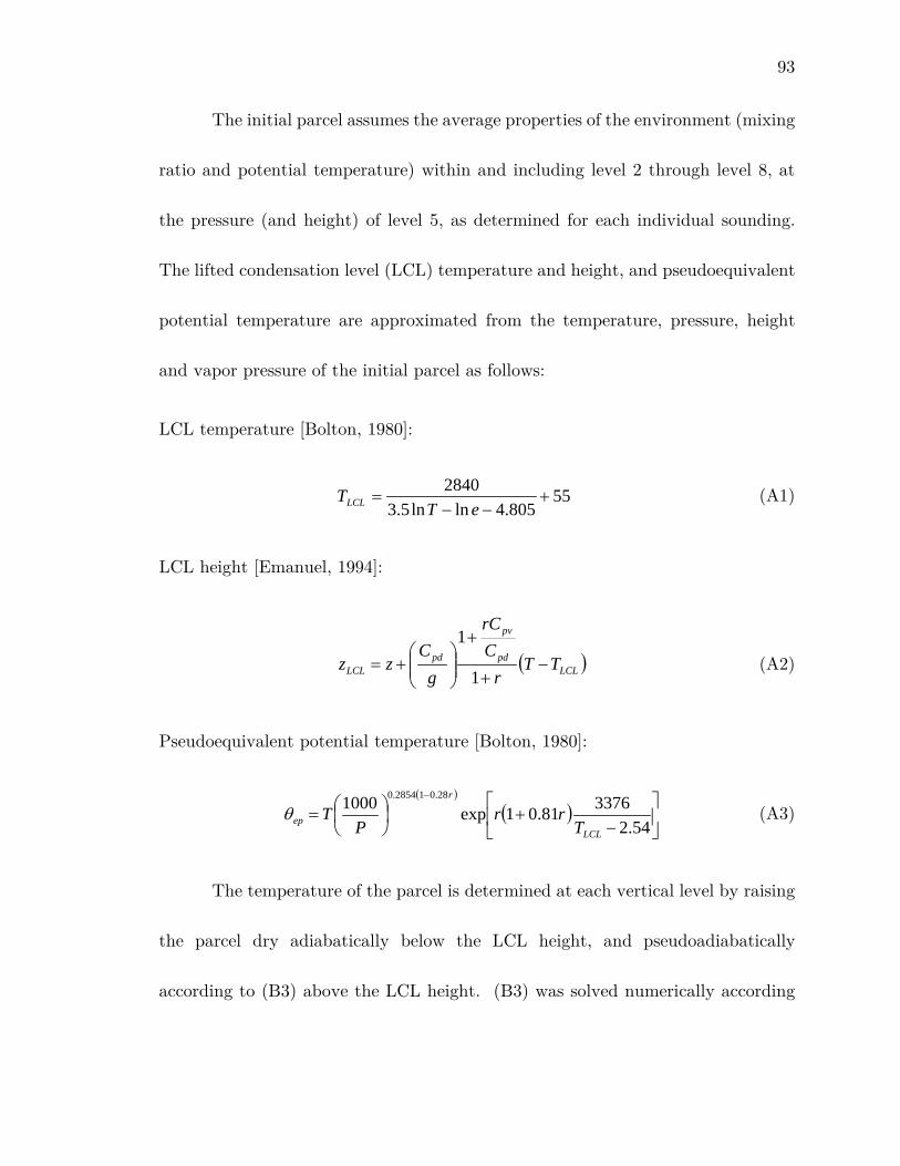
93
The initial parcel assumes the average properties of the environment (mixing
ratio and potential temperature) within and including level 2 through level 8, at
the pressure (and height) of level 5, as determined for each individual sounding.
The lifted condensation level (LCL) temperature and height, and pseudoequivalent
potential temperature are approximated from the temperature, pressure, height
and vapor pressure of the initial parcel as follows:
LCL temperature [Bolton, 1980]:
55805.4lnln5.3
2840+
−−=
eTTLCL (A1)
LCL height [Emanuel, 1994]:
( )LCLpd
pv
pdLCL TT
rCrC
gC
zz −+
+
+=
1
1 (A2)
Pseudoequivalent potential temperature [Bolton, 1980]:
( )
( )
−
+
=
−
54.2337681.01exp1000 28.012854.0
LCL
r
ep Trr
PTθ (A3)
The temperature of the parcel is determined at each vertical level by raising
the parcel dry adiabatically below the LCL height, and pseudoadiabatically
according to (B3) above the LCL height. (B3) was solved numerically according
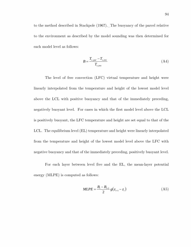
94
to the method described in Stackpole (1967). The buoyancy of the parcel relative
to the environment as described by the model sounding was then determined for
each model level as follows:
envv
envvparv
TTT
B,
,, −= (A4)
The level of free convection (LFC) virtual temperature and height were
linearly interpolated from the temperature and height of the lowest model level
above the LCL with positive buoyancy and that of the immediately preceding,
negatively buoyant level. For cases in which the first model level above the LCL
is positively buoyant, the LFC temperature and height are set equal to that of the
LCL. The equilibrium level (EL) temperature and height were linearly interpolated
from the temperature and height of the lowest model level above the LFC with
negative buoyancy and that of the immediately preceding, positively buoyant level.
For each layer between level five and the EL, the mean-layer potential
energy (MLPE) is computed as follows:
( )iiii zzgBBMLPE −
−= +
+1
1
2 (A5)
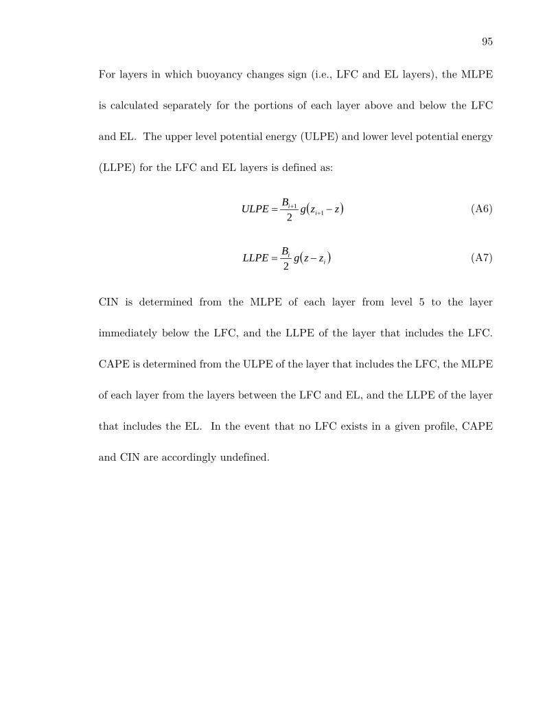
95
For layers in which buoyancy changes sign (i.e., LFC and EL layers), the MLPE
is calculated separately for the portions of each layer above and below the LFC
and EL. The upper level potential energy (ULPE) and lower level potential energy
(LLPE) for the LFC and EL layers is defined as:
( )zzgBULPE ii −= ++
11
2 (A6)
( )ii zzgBLLPE −=
2 (A7)
CIN is determined from the MLPE of each layer from level 5 to the layer
immediately below the LFC, and the LLPE of the layer that includes the LFC.
CAPE is determined from the ULPE of the layer that includes the LFC, the MLPE
of each layer from the layers between the LFC and EL, and the LLPE of the layer
that includes the EL. In the event that no LFC exists in a given profile, CAPE
and CIN are accordingly undefined.
96
Appendix B: Uncertainty equations for cloud microphysical properties
Cloud Water Phase Partition
The following simple mixed-mode fractionating scheme based on MSecmwf
high-resolution temperature profiles is used to determine ice fraction 𝑖𝑖 and liquid
water fraction ℓ which separate the total measured radar reflectivity factor
𝑍𝑍T [mm6 m−3] into ice and liquid water portions (𝑍𝑍i and 𝑍𝑍ℓ , respectively) for
temperatures between -16 and 0°C :
𝑖𝑖 = −𝑇𝑇/16
ℓ = 1 − 𝑖𝑖 = 1 + 𝑇𝑇/16
𝑍𝑍i = 𝑖𝑖𝑍𝑍T = −𝑇𝑇
16𝑍𝑍T
𝑍𝑍ℓ = ℓ𝑍𝑍T = �1 +𝑇𝑇
16� 𝑍𝑍T
Ice Water Content
97
Ice water content (IWC) is determined from Zi by the empirical relationship
of Liu and Illingworth (2000):
IWC = 0.097𝑍𝑍i0.59 = 0.097 �−𝑇𝑇
16𝑍𝑍T�
0.59
The uncertainty in IWC based on the uncertainty in temperature 𝛿𝛿𝑇𝑇 is given by:
𝛿𝛿IWC =𝑑𝑑IWC𝑑𝑑𝑇𝑇
𝛿𝛿𝑇𝑇 = 0.097 �𝑍𝑍𝑇𝑇16�0.59 𝑑𝑑
𝑑𝑑𝑇𝑇(−𝑇𝑇)0.59𝛿𝛿𝑇𝑇 = −0.05723
�𝑍𝑍𝑇𝑇16�0.59
(−𝑇𝑇)0.41 𝛿𝛿𝑇𝑇
Ice Cloud Particle Effective Radius
Ice cloud particle effective radius (𝑟𝑟𝑒𝑒𝑖𝑖) is a function of temperature according
to Ivanova et al. (2001):
𝑟𝑟𝑒𝑒𝑖𝑖 =75.3 + 0.5895𝑇𝑇
2
The uncertainty in 𝑟𝑟𝑒𝑒𝑖𝑖 based on the uncertainty in temperature 𝛿𝛿𝑇𝑇 is given by:
𝛿𝛿𝑟𝑟𝑒𝑒𝑖𝑖 =𝑑𝑑𝑟𝑟𝑒𝑒𝑖𝑖𝑑𝑑𝑇𝑇
𝛿𝛿𝑇𝑇 =𝑑𝑑𝑑𝑑𝑇𝑇
�75.3 + 0.5895𝑇𝑇
2� 𝛿𝛿𝑇𝑇 = 0.29475 𝛿𝛿𝑇𝑇
Liquid Water Content
98
Liquid water content (LWC) is based on Zl and an assumed reference cloud particle
number N0 of 100 cm-3, as derived by Liao and Sassen (1994):
LWC = �𝑁𝑁0𝑍𝑍ℓ3.6
�5/9
= �𝑁𝑁0 �1 + 𝑇𝑇
16�𝑍𝑍T3.6
�
5/9
The uncertainty in LWC based on the uncertainty in temperature 𝛿𝛿𝑇𝑇 is given by:
𝛿𝛿LWC =𝑑𝑑LWC𝑑𝑑𝑇𝑇
𝛿𝛿𝑇𝑇 = �𝑁𝑁0𝑍𝑍T3.6
�5/9 𝑑𝑑
𝑑𝑑𝑇𝑇�1 +
𝑇𝑇16�5/9
𝛿𝛿𝑇𝑇 =5 �𝑁𝑁0𝑍𝑍T3.6 �
5/9
144 �1 + 𝑇𝑇16�
4/9 𝛿𝛿𝑇𝑇
Liquid Water Effective Radius
Liquid water effective radius (𝑟𝑟𝑒𝑒) is a function of the LWC, assuming a log-normal
droplet distribution with a width σ of 0.35 and cloud particle number concentration
Nd equal to 200 cm-3 according to Frisch et al. (1995):
𝑟𝑟𝑒𝑒 = 1.358 �3LWC
4𝜋𝜋𝜌𝜌𝑤𝑤𝑁𝑁𝑑𝑑exp �9𝜎𝜎22 �
�
1/3
The uncertainty in 𝑟𝑟𝑒𝑒 based on the uncertainty in temperature 𝛿𝛿𝑇𝑇 is given by:
𝛿𝛿𝑟𝑟𝑒𝑒 =𝑑𝑑𝑟𝑟𝑒𝑒𝑑𝑑𝑇𝑇
𝛿𝛿𝑇𝑇 = 1.358𝑑𝑑𝑟𝑟𝑚𝑚𝑑𝑑𝑇𝑇
= 1.358𝑑𝑑𝑟𝑟𝑚𝑚𝑑𝑑LWC
𝑑𝑑LWC𝑑𝑑𝑇𝑇
99
𝑑𝑑𝑟𝑟𝑚𝑚𝑑𝑑LWC
=13�
3
4𝜋𝜋𝜌𝜌𝑤𝑤𝑁𝑁𝑑𝑑exp �9𝜎𝜎22 �
�
1/3
LWC−2/3 =13�
3
4𝜋𝜋𝜌𝜌𝑤𝑤𝑁𝑁𝑑𝑑exp �9𝜎𝜎22 �
�
1/3
�𝑁𝑁0 �1 + 𝑇𝑇
16�𝑍𝑍T3.6
�
−10/27
𝛿𝛿𝑟𝑟𝑒𝑒 =1.358
3�
3
4𝜋𝜋𝜌𝜌𝑤𝑤𝑁𝑁𝑑𝑑exp �9𝜎𝜎22 �
�
1/3
�𝑁𝑁0 �1 + 𝑇𝑇
16�𝑍𝑍T3.6
�
−10/27
�5 �𝑁𝑁0𝑍𝑍T3.6 �
5/9
144 �1 + 𝑇𝑇16�
4/9� 𝛿𝛿𝑇𝑇
𝛿𝛿𝑟𝑟𝑒𝑒 =6.79432
�3
4𝜋𝜋𝜌𝜌𝑤𝑤𝑁𝑁𝑑𝑑exp �9𝜎𝜎22 �
�
1/3
�𝑁𝑁0𝑍𝑍T3.6 �5/27
�1 + 𝑇𝑇16�
22/27 𝛿𝛿𝑇𝑇
100
Appendix C: Simulated Seasonal Cycles of Rainfall in the Region Surrounding Niamey
The evolution of monthly-mean rainfall rate derived from measurements recorded
by the AMF-1 PWD during 2006 in Niamey, Niger are compared to the 2006 –
2015 envelopes of minimum and maximum monthly-average rainfall rate simulated
by GISS-E2-R for the grid cell containing Niamey (Fig. D.1-e) and the eight
surrounding grid cells (Fig. D.1-a, b, c, d, f, g, h, i). Consistent with the spatial
distribution of annual rainfall totals reported by Lélé and Lamb (2010), GISS-E2-
R simulates higher monthly-average rainfall rates (indicating larger monthly
accumulated rainfall totals) throughout the monsoon season to the south and east
of the grid cell containing Niamey, while lower monthly-average rainfall rates are
produced to the north and east of the grid cell containing Niamey. GFDL-CM3
produces a similar pattern of monthly-mean rainfall rates (Fig. D.2). It is therefore
concluded that spatial displacement is not a significant source of error in the
monthly average rainfall rates simulated by these two models for the grid cell
including Niamey.
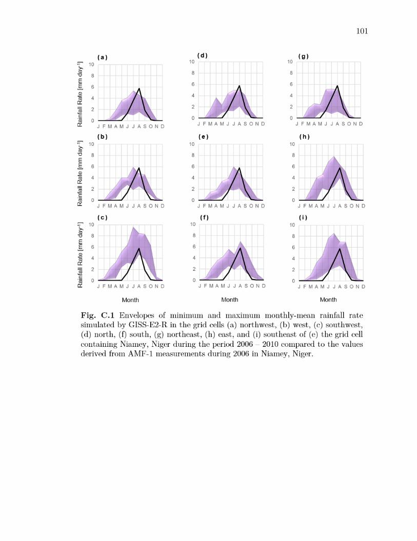
101
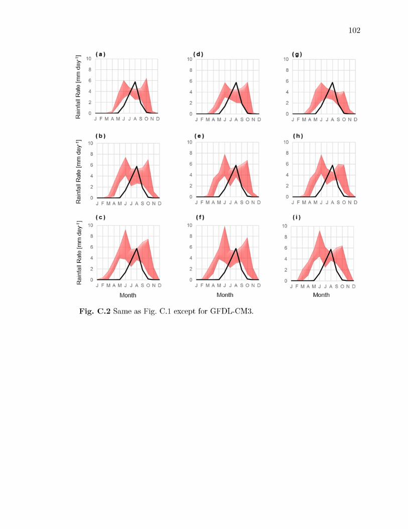
102
103
References
Askne, J. I. H., and E. R. Westwater, 1986: A review of ground-based remote
sensing of temperature and humidity by passive microwave radiometers. IEEE
Transactions on Geoscience and Remote Sensing, GE-24, 340-352.
Augustine, J.A., J.J. DeLuisi, and C.N. Long, 2000: SURFRAD – A national
surface radiation budget network for atmospheric research. Bull. Amer. Meteor.
Soc. 133, 1993-2010.
Biasutti, M., I. M. Held, A. H. Sobel, and A. Giannini, 2008: SST forcings and
Sahel rainfall variability in simulations of the twentieth and twenty-first
centuries. J. Climate, 21, 3471– 3486.
Bolton, D., 1980: The computation of equivalent potential temperature. Mon.
Wea. Rev., 108, 1046-1053.
Bony, S., and J-L. Dufresne, 2005: Marine boundary layer clouds at the heart of
tropical cloud feedback uncertainties in climate models. Geophys. Res. Lett., 32,
L20806.
Cadeddu, M. P., J. C. Liljegren, and D. D. Turner, 2013: The atmospheric
radiation measurement (ARM) program network of microwave radiometers:
instrumentation, data, and retrievals. Atmos. Meas. Tech., 6, 2359-2372.
Christensen, J.H., K. Krishna Kumar, E. Aldrian, S.-I. An, I.F.A. Cavalcanti, M.
de Castro, W. Dong, P. Goswami, A. Hall, J.K. Kanyanga, A. Kitoh, J. Kossin,
N.-C. Lau, J. Renwick, D.B. Stephenson, S.-P. Xie and T. Zhou, 2013: Climate
104
Phenomena and their Relevance for Future Regional Climate Change. In:
Climate Change 2013: The Physical Science Basis. Contribution of Working
Group I to the Fifth Assessment Report of the Intergovernmental Panel on
Climate Change [Stocker, T.F., D. Qin, G.-K. Plattner, M. Tignor, S.K. Allen,
J. Boschung, A. Nauels, Y. Xia, V. Bex and P.M. Midgley (eds.)]. Cambridge
University Press, Cambridge, United Kingdom and New York, NY, USA, pp.
1217–1308, doi: 10.1017/CBO9781107415324.028.
Cimini, D., T. Hewison, L. Martin, J. Güldner, C. Gaffard, and F. Marzano, 2006:
Temperature and humidity profile retrievals from ground-based microwave
radiometers during TUC. Meteor. Z., 15, 45-56, doi:10.1127/0941-
2948/2006/0099.
Collow, A. B., Ghate, V. P., Miller, M. A. and Trabachino, L. C. (2016), A one-
year study of the diurnal cycle of meteorology, clouds and radiation in the West
African Sahel region. Q.J.R. Meteorol. Soc., 142: 16–29. doi: 10.1002/qj.2623
Cook, K.H., and E.K. Vizy, 2006: Coupled model simulations of the West African
monsoon system: Twentieth- and twenty-first century simulations. J. Climate,
19, 3681 – 3703.
Cook, D.R. and M.S. Pekour, 2008: Eddy correlation flux measurement system
handbook. Tech. Rep. DOE/SC-ARM/TR-05I, Off. of Biol. and Environ. Res.,
Off. of Sci., U.S. Dep. of Energy, Washington, D.C.
Del Genio, A.D. and M.-S. Yao, 1993: Efficient cumulus parameterization for long-
term climate studies: The GISS scheme. The Representation of Cumulus
105
Convection in Numerical Models, AMS Meteorol. Monogr., vol. 46, edited by
K.A. Emanueal and D.A. Raymond, pp. 181-184, Am. Meteorol Soc.,
Washington, D.C.
Del Genio, A.D., M.-S. Yao, W. Kovari, and K.K. Lo, 1996: A prognostic cloud
water parameterization for general circulation models. J. Climate, 9, 270-304.
Del Genio, A.D., M.-S. Yao, and J. Jonas, 2007: Will moist convection be stronger
in a warmer climate? Geophys. Res. Lett., 34, L16703, doi:
10.1029/2007/GL030525.
Delworth, T.L., et al., 2006: GFDL’s CM2 global coupled climate models. Part I:
Formulation and simulation characteristics. J. Climate, 19, 643-674.
Diffenbaugh, N.S., and F. Giorgi, 2012: Climate change hotspots in the CMIP5
global climate model ensemble. Climate Change, 114(3-4), 813-822.
Donner, L.J., 1993: A cumulus parameterization including mass fluxes, vertical
momentum dynamics, and mesoscale effects. J. Atmos. Sci., 50, 889-906.
Donner L.J., C.J. Seman, R.S. Hemler, and S. Fan, 2001: A cumulus
parameterization including mass fluxes, convective vertical velocities, and
mesoscale effects: Thermodynamic and hydrological aspects in a general
circulation model. J. Climate, 14, 3444-3463.
Donner, Leo J., Bruce Wyman, Richard S Hemler, Larry W Horowitz, Yi Ming,
Ming Zhao, J-C Golaz, Paul Ginoux, Shian-Jiann Lin, M Daniel Schwarzkopf,
John Austin, G Alaka, W F Cooke, Thomas L Delworth, Stuart Freidenreich,
106
C Tony Gordon, Stephen M Griffies, Isaac M Held, William J Hurlin, Stephen
A Klein, Thomas R Knutson, Amy R Langenhorst, H C Lee, Y Lin, B I Magi,
Sergey Malyshev, P C D Milly, Vaishali Naik, Mary Jo Nath, R Pincus, Jeff J
Ploshay, V Ramaswamy, Charles J Seman, Elena Shevliakova, Joseph J Sirutis,
William F Stern, Ronald J Stouffer, R John Wilson, Michael Winton, Andrew
T Wittenberg, and Fanrong Zeng, July 2011: The dynamical core, physical
parameterizations, and basic simulation characteristics of the atmospheric
component AM3 of the GFDL Global Coupled Model CM3. J.
Climate, 24(13), doi:10.1175/2011JCLI3955.1.
Druyan, L.M., 1991: The sensitivity of Sub-Saharan precipitation to Atlantic SST.
Climate Change, 18, 17-36.
Dunn, M, K. Johnson, and M. Jensen, 2011: The microbase value-added product:
a baseline retrieval of cloud microphysical properties. U.S. Department of
Energy. DOE/SC-ARM/TR-095.
Eldridge, R.H., 1957: A synoptic study of West African disturbance lines. Quart.
J. Roy. Meteor. Soc., 83, 303-314.
Emanuel, K., 1994: "Atmospheric Convection". Oxford University Press, New
York, 580 pp.
107
Han, Y. and E. R. Westwater, 2003: Analysis and improvement of tipping
calibration for ground-based microwave radiometers. IEEE Transactions on
Geoscience and Remote Sensing, GRS-38, 1260-1277.
Flato, G., J. Marotzke, B. Abiodun, P. Braconnot, S.C. Chou, W. Collins, P. Cox,
F. Driouech, S. Emori, V. Eyring, C. Forest, P. Gleckler, E. Guilyardi, C. Jakob,
V. Kattsov, C. Reason and M. Rummukainen, 2013: Evaluation of Climate
Models. In: Climate Change 2013: The Physical Science Basis. Contribution of
Working Group I to the Fifth Assessment Report of the Intergovernmental Panel
on Climate Change [Stocker, T.F., D. Qin, G.-K. Plattner, M. Tignor, S.K.
Allen, J. Boschung, A. Nauels, Y. Xia, V. Bex and P.M. Midgley (eds.)].
Cambridge University Press, Cambridge, United Kingdom and New York, NY,
USA.
Fontaine B, Roucou P, Monerie P-A. 2011. Changes in the African monsoon region
at medium-term time horizon using 12 AR4 coupled models under the A1b
emissions scenario. Atmospheric Science Letters, 12, 83–88, DOI:
10.1002/asl.321.
Frisch, A.S., C. W. Fairall, and J. B. Snider, 1995: Measurements of stratus cloud
and drizzle parameters in ASTEX with a Ka-Band Doppler radar and a
microwave radiometer. J. Atmos. Sci., 52, 2788-2799.
Garnache, R. R. and J. Fisher, 2003: Half-widths of H216O, H218O, H217O,
HD16O, and D216O: I. Comparison between isotopomers. J. Quant. Spectrosc.
Radiat. Transfer, 78, 289-304.
108
GFDL Global Atmospheric Model Development Team, 2004: The new GFDL
global atmosphere and land model AM2/LM2: Evaluation with prescribed SST
simulations. J. Climate, 17, 4641-4673.
Grabowski, W., 2001: Coupling cloud processes with the large-scale dynamics using
the cloud-resolving convection parameterization (CRCP). J. Atmos. Sci, 58,
978-997.
Güldner, J. and D. Spänkuch, 2001: Remote sensing of the thermodynamic state
of the atmospheric boundary layer by ground-based microwave radiometry. J.
Atmos. Oceanic Technol.,18, 925-933.
Harries, J.E., and Coauthors, 2005: The Geostationary Earth Radiation Budget
project. Bull. Amer. Meteorol. Soc., 86, 945-960.
Ianova, D.D., L. Mitchell, W. P. Arnott, and M. Poellot, 2001: A GCM
parameterization for bimodal size spectra and ice mass removal rates in mid-
latitude cirrus clouds. Atmos. Res., 59, 89-113.
Ilesanmi, O.O., 1971: An empirical formulation of an ITD rainfall model for the
tropics: A case study of Nigeria. J. Appl. Meeor., 10, 882-891.
Illingworth, A., and S. Bony, 2009: Observational Strategies at Meso- and Large
Scales to Reduce Critical Uncertainties in Future Cloud Changes. Clouds in the
Perturbed Climate System, J. Heintzenberg and R.J. Charlson, Eds., MIT Press,
511-530.
IPCC, 2013: Summary for Policymakers. In: Climate Change 2013: The Physical
Science Basis. Contribution of Working Group I to the Fifth Assessment Report
109
of the Intergovernmental Panel on Climate Change [Stocker, T.F., D. Qin, G.-
K. Plattner, M. Tignor, S. K. Allen, J. Boschung, A. Nauels, Y. Xia, V. Bex and
P.M. Midgley (eds.)]. Cambridge University Press, Cambridge, United Kingdom
and New York, NY, USA.
Jakob, Christian, 2010: Accelerating Progress in Global Atmospheric Model
Development through Improved Parameterizations: Challenges, Opportunities,
and Strategies. Bull. Amer. Meteor. Soc., 91, 869–875.
Kim, D., A. Del Genio, and M.-S. Yao, 2011: Moist convection scheme in ModelE2.
Technical report, NASA Goddard Inst. for Space Stud. arXiv:1312.7496.
Kim, D., H. Sobel, A.D. Del Genio, Y.-H. Chen S.J. Camargo, M.S. Yao, M. Kelley,
and L. Nazarenko, The tropical subseasonal variability simulated in the NASA
GISS general circulation model. J. Climate., 25, 4641-4659, doi: 10.1175/JCLI-
D-11-00447.1.
Knupp, K. R., R. Ware, D. Cimini, F. Vandenberghe, J. Vivekanandan, E.
Westwater, T. Coleman, and D. Phillips, 2009: Ground-based passive microwave
profiling during dynamic weather conditions. J. Atmos. Oceanic Tech., 26,
1057-1073, doi: 10.1175/2008JTECHA1150.1
Kollias, P., M. A. Miller, K. L. Johnson, M. P. Jensen, and D. Troyan, 2009: Cloud,
thermodynamic, and precipitation observations in West Africa during 2006. J.
Geophys. Res., 114, D00E08, doi:10.1029/2008JD010641.
Lélé, M.I., and P.J. Lamb, 2010: Variability of the Intertropical Front (ITF) and
rainfall over the West African Sudan-Sahel Zone. J. Climate., 23, 3984 – 4004.
110
Liao, L. and K. Sassen, 1994: Investigation of relationships between Ka-Band
radar reflectivity and ice and liquid water contents. Atmos. Res., 34, 231-248.
Liljegren, J. C., B. M. Lesht, S. Kato, and E. Clothiaux, 2001a: Initial evaluation
of profiles of temperature, water vapor, and cloud liquid water from a new
microwave profiling radiometer. Proc. 11th Symposium on Meteorological
Observations and Instrumentation, Albuquerque, NM, Amer. Meteor. Soc., 8.6.
Liljegren, J. C., B. Lesht, S. Kato, and. E. Clothiax, 2001b: "Initial evaluation of
profiles of temperature, water vapor, and cloud liquid water from a new
microwave profiling radiometer", presented at the 11th Atmospheric Radiation
Measurement (ARM) Program Science Team Meeting, Atlanta, GA, 19-23
March 2001.
Liljegren, J. C., S. Boukabara, K. Cady-Pereira, and S. A. Clough, 2005: The
effect of the half-width of the 22-GHz water vapor line on retrievals of
temperature and water vapor profiles with a 12-channel microwave radiometer.
IEEE Transactions on Geoscience and Remote Sensing, 43, 1102 - 1108.
Liu, C. L. and A. J. Illingworth, 2000: Toward more accurate retrievals of ice
water content from radar measurements of clouds. J. Applied. Meteorol.,39,
1130-1146.
Martin, G.M., M.A. Ringer, V.D. Pope, A. Jones, C.Dearden, and T.J. Hinton,
2006: The physical properties of the atmosphere in the new Hadley Centre
Global Environmental Model, HadGEM1. Part I: Model description and global
climatology. J. Climate, 19, 1274-1301.
111
Mather, J.H., and J.W. Voyles, 2013: The ARM climate research facility: A review
of structure and capabilities. Bull. Am. Meteorol. Soc. 94, 377 – 392.
Meehl, G.A., C. Covey, T. Delworth, M. Latif, B. McAvaney, J.F.B. Mitchell, R.J.
Stouffer, and K.E. Taylor, 2007: The WCRP CMIP3 multi-model dataset: A
new era in climate change research. Bull. Amer. Meteor. Soc., 88, 1383-1394.
Miller, M., V. Ghate, and R. Zahn, 2012: The radiation budget of the West African
Sahel and its controls: A perspective from observations and global climate
models. J. Climate. 25, 5976-5996, doi:10.1175/JCLI-D-11-00072.1.
Miller, R. L., A. Slingo, J.C. Barnard, and E. Kassianov, 2009: Seasonal contrast
in the surface energy balance of the Sahel. J. Geophys. Res., 114, D00E05.
Miller, M. A., and A. Slingo, 2007: The ARM Mobile Facility and its first
international deployment: Measuring radiative flux divergence in West Africa.
Bull. Amer. Meteor. Soc., 88, 1229-1244, doi: 10.1175/BAMS-88-8-1229.
Monkam, D., 2002: Convective available potential energy (CAPE) in northern
Africa and tropical Atlantic: A study of it connections with rainfall in central
and west Africa during summer 1985. Atmos. Res., 62, 125-147.
Mlawer, E. J., S. A. Clough, and D. C. Tobin, 2003: "The MT_CKD water vapor
continuum: A revised perspective including collision induced effects", presented
at the Atmospheric Science from Space using Fourier Transform Spectroscopy
(ASSFTS) Workshop, Bad Wildbad (Black Forest), Germany, 8-10 October
2003.
112
Mora, C.F., A.G., R.J. Longman, R.S. Dacks, M.M. Walton, E.J. Tong, J.J.
Sanchez, L.R. Kiaser, Y.O. Stender, J.M. Anderson, C.M. Ambrosino, I.
Fernandez-Silva, L.M. Gluseffi, and T.W. Giambelluca, 2013: The projected
timing of climate departure from recent variability. Nature, 502, 183-187.
Niang, I., O.C. Ruppel, M.A. Abdrabo, A. Essel, C. Lennard, J. Padgham, and P.
Urquhart, 2014: Africa. In: Climate Change 2014: Impacts, Adaptation, and
Vulnerability. Part B: Regional Aspects. Contribution of Working Group II to
the Fifth Assessment Report of the Intergovernmental Panel on Climate
Change [Barros, V.R., C.B. Field, D.J. Dokken, M.D. Mastrandrea, K.J. Mach,
T.E. Bilir, M. Chatterjee, K.L. Ebi, Y.O. Estrada, R.C. Genova, B. Girma,
E.S. Kissel, A.N. Levy, S. MacCracken, P.R. Mastrandrea, and L.L. White
(eds.)]. Cambridge University Press, Cambridge, United Kingdom and New
York, NY, USA, pp. 1199-1265.
Randall, D.A., M. Khairoutdinov, A. Araawa, and W. Grabowski, 2003: Breaking
the cloud parameterization deadlock. Bull. Amer. Meteor. Soc., 84, 1547-1564.
Randall, D.A, R.A. Wood, S. Bony, R. Colman, T. Fichefet, J. Fyfe, V. Kattsov,
A. Pitman, J. Shukla, J. Srinivasan, R.J. Stouffer, A. Sumi and K.E. Taylor,
2007: Climate Models and Their Evaluation. In: Climate Change 2007: The
Physical Science Basis. Contribution of Working Group I to the Fourth
Assessment Report of the Intergovernmental Panel on Climate Change
[Solomon, S., D. Qin, M. Manning, Z. Chen, M. Marquis, K.B. Averyt, M.
Tignor and H.L. Miller (eds.)]. Cambridge University Press, Cambridge, United
Kingdom and New York, NY, USA
113
Revercomb, H. and Coauthors, 2003: The ARM program’s water vapor intensive
observation periods. Bull. Am. Meteor. Soc. 84, 217 – 236.
Roehrig, R., D. Bouniol, F. Guichard, F. Hourdin, and J.-L. Redelsperger, 2013:
The present and future of the West African monsoon: A process-oriented
assessment of CMIP5 simulations along the AMMA transect. J. Climate, 26,
6471 – 6505, doi: 10.1175/JCLI-D-12-00505.1.
Rosenkranz, P., 1998: Water vapor continuum absorption: A comparison of
measurements and models. Radio Sci., 33, 919-928.
Russell, G.L., J.R. Miller, and D. Rind, 1995: A coupled atmosphere-ocean model
for transient climate change studies. Atm.-Ocean, 33(4), 683-730.
Satoh, M., T. Matsuno, and H. Tomita et al., 2008: Nonhydrostatic icosaherdral
atmospheric model (NICAM) for global cloud-resolving simulations. J. Comp.
Phys., 227, 3486-3514.
Schmetz, J., P. Pili, S. Tjemkes, D. Just, J. Kerkmann, S. Rota, and A. Ratier,
2002: An introduction to Meteosat Second Generation (MSG). Bull. Amer.
Meteor. Soc., 83, 977-992.
Schmidt et al., 2006: Present-day atmospheric simulations using GISS ModelE:
Comparison to in situ, satellite, and reanalysis data. J. Climate, 19, 153-192
Schmidt G.A., et al., 2014: Configuration and assessment of the GISS ModelE2
contributions to the CMIP5 archive. J. Adv. Model. Earth Syst., 6, 141-184, doi:
10.1002/2013MS000265.
114
Schroeder, J. A. and E. R. Westwater, 1991: "Users Guide to WPL Microwave
Radiative Transfer Software," Report ERL-WPL-213, NOAA Environmental
Research Laboratory, Boulder, CO.
Settle, J.J., N.A. Bharmal, G.J. Robinson, and A. Slingo, 2008: Sampling
uncertainties in surface radiation budget calculations in RADAGAST. J.
Geophys. Res., 113, D00E02, doi: 10.1029/2008JD010509.
Siebesma, A.P., and Coauthors, 2009: Cloud-controlling Factors. Clouds in the
Perturbed Climate System, J. Heintzenberg and R.J. Charlson, Eds., MIT Press,
269-290.
Slingo, A., et al., 2008: Overview of observations from the RADAGAST
experiment in Niamey, Niger: 1. Meteorological and thermodynamic variables.
J. Geophys. Res., 113, D00E01, doi: 10.1029/2008JD009909.
Slingo, A., H.E. White, N.A. Bharmal, and G.J. Robinson, 2009: Overview of
observations from the RADAGAST experiment in Niamey, Niger: 2. Radiative
fluxes and divergences. J. Geophys. Res., 114, D00E04, doi:
10.1029/2008JD010497.
Solheim F., J. Godwin, and R. Ware, 1998a: Passive ground-based remote sensing
of atmospheric temperature, water vapor, and cloud liquid water profiles by a
frequency synthesized microwave radiometer. Meterologische Zeitschrift, N. F.,
7, 370-376.
Solheim, F., J. R. Godwin, E. R. Westwater, Y. Han, S. J. Keihm. K. Marsh, and
R. Ware, 1998b: Radiometric profiling of temperature, water vapor and cloud
liquid water using various inversion methods. Radio Sci., 33, 393-404.
115
Stackpole, J. D., 1967: Numerical analysis of atmospheric soundings. J. Appl.
Meteor., 24, 640-657.
Stephens, G.L., 2005: Cloud feedbacks in the climate system: a critical review. J.
Climate, 17, 3661-3665.
Stoffel, T., 2005: Solar Infrared Radiation Station (SIRS) handbook. ARM TR-
025. Department of Energy, Washington DC, 29 pp. [Available online at
http://www.arm.gov]
Trabachino, L. and M.A. Miller, 2014: Thermodynamic profiling capabilities of
the microwave radiometer profiler in various locations of interest for atmospheric
model development. In Atmospheric System Research Science Team Meeting,
10-14 March 2014, Potomac, MD.
Troyan, D., 2012: Merged Sounding Value-Added Product Technical Report. U.S.
Department of Energy. DOE/SC-ARM-TR-102.
Ware, R., R. Carpenter, J. Güldner, J. Liljegren, T. Nehrkorn, F. Solheim, and F.
Vandenberghe, 2003: A multichannel radiometer profiler of temperature,
humidity, and cloud liquid. Radio Sci., 38, 8079, doi:10.1029/2002RS002856.
Westwater, E. R., Y Han, and F. Solheim, 2000: Resolution and accuracy of a
multi-frequency scanning radiometer for temperature profiling. Microw.
Radiomet. Remote Sens. Earth's Surf. Atmosphere, P. Pampaloni and S.
Paloscia (Eds.), pp. 129-135.
116
Wilcox E.M., and L.J. Donner, 2007: The frequency of extreme rain events in
satellite rain-rate estimates and an atmospheric general circulation model. J.
Climate, 20, 53-69.
Williams, K.D., and G. Tselioudis, 2007: GCM intercomparisons of global cloud
regimes: Present-day evaluation and climate change response. Climate Dyn.,
20, 231-250.
Williams, K.D. and M.J. Webb, 2008: A quantitative performance assessment of
cloud regimes in climate models. Clim. Dyn., 33, 141-157.