Thu 3/31/2016Representation of clouds and precipitation:

- WRF scheme options + some background- Sensitivity to CCN:

- Convective storm case study- Stratus dissipation problem

Reminders/announcements:• MP paper summary assignment• Upcoming: MP experiments• Tuesday 4/5: Class will not meet, but recorded lecture will

be posted on www page

MP papers: Will do sign-up sheet

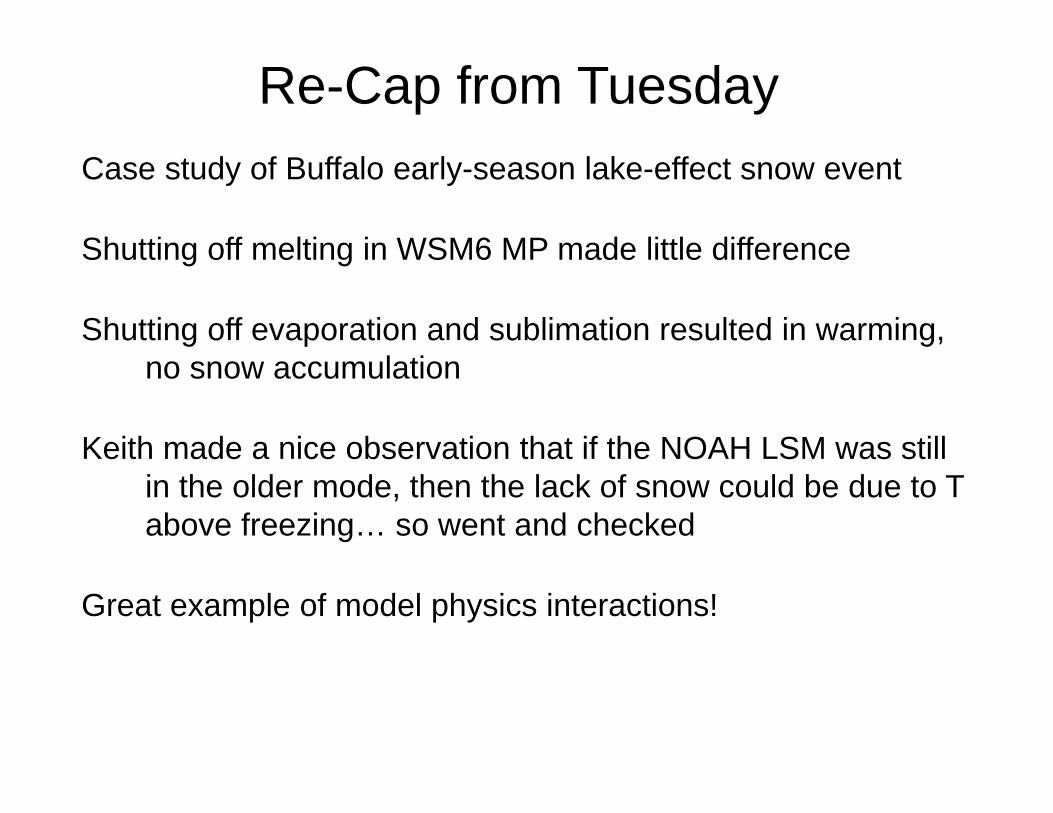
Re-Cap from TuesdayCase study of Buffalo early-season lake-effect snow event

Shutting off melting in WSM6 MP made little difference

Shutting off evaporation and sublimation resulted in warming, no snow accumulation

Keith made a nice observation that if the NOAH LSM was still in the older mode, then the lack of snow could be due to T above freezing… so went and checked

Great example of model physics interactions!

Little difference in T between NOMELT, control

Up to 1.5 C warmer in NOEVAP than control

No snow in NOEVAP

• similar amount of precipitation, too warm to be snow

Similar snowfall amounts in NOEVAP, control

noevap

control

nomelt

2-meter T at Buffalo

Model snowfall rate at Buffalo

NOAH LSM, then and now

WRFV2.2 NOAH LSM:

WRFV371 NOAH LSM:

A partial listing of microphysical processes

Deposition/sublimation of graupel Melting of hail

Deposition/sublimation of cloud ice Homogeneous freezing of cloud water

Deposition/sublimation of snow Homogeneous freezing of rain water

Deposition on ice nuclei (nucleation) Accretion of cloud water to graupel

Deposition/sublimation of hail Accretion of cloud water to snow (rime)

Condensation/evaporation of cloud water Coalescence of cloud water to rain

Condensation/evaporation of rain water Cloud water to rain (autoconversion)

Freezing of cloud water (immersion, contact) Accretion of cloud ice by snow

Freezing of rain water (immersion, contact) Accretion of snow by snow (aggregation)

Melting of cloud ice Accretion of cloud ice by graupel

Melting of snow Accretion of rain water to graupel

Melting of graupel Accretion of snow by graupel

Breakup of rain drops Splintering of freezing droplets

Breakup of snow crystals Accretion of snow by rain

WRF MP Options (first 11 of 22) (V3.7.1)

mp_physics Characteristics Design

1: Kessler Bulk, single moment, 3 class Simplest possible, use for test case

2: Lin Bulk, single moment, 6 class Classic, ahead of its time. WSM6 updates

3: WSM3 Bulk, single moment, 3 class, simple ice All ice below freezing, all warm above

4: WSM5 Bulk, single moment, 5 class Probably okay for coarse grid spacing

5: Ferrier Bulk, single moment, NAM scheme Clever total ice advection for efficiency

6: WSM6 Bulk, single moment, 6 class, can add hail An updated Lin et al., standard/default

7: Goddard Bulk, single moment, 6 class, hail option Can set switch to have hail vs. graupel

8: Thompson Bulk, 6-class, double moment for ice, rain Computationally efficient part double moment

9: Milbrandt-Yau Bulk, 7-class, double moment for all Expensive. Double moment, fixed alpha

10: Morrison Bulk, 6-class, double moment for cloud ice, cloud water, rain, and snow. Can add hail

Designed for arctic clouds, good radiation int.

11: CAM 5.1 Bulk, 5-class, double moment, NEW in WRF Some aspects not fully implemented in WRF

WRF MP Options (through 22)

mp_physics Characteristics Design

13: SBU_Ylin Bulk, single-moment, 5-class, diagnosed riming intensity – continuous spectrum

No cutoff distinction between graupel/snow

14: WDM5 Bulk, single moment, 3 class Perhaps useful in special cases

16: WDM6 Bulk, single moment, 6 class, can add hail Double moment for CCN, cloud, rain

17: NSSL 2/4 Bulk, NSSL double moment 4 ice All NSSL schemes allow setting intercept

18: NSSL CCN Bulk, double moment, predicted CCN For double moment, can set shape param.

19: NSSL single 7 Bulk, single moment, 7 class Predicts graupel

21: NSSL single 6 Bulk, single moment, 6 class, set intercepts Can set many namelist parameters

28: Thompson AA Bulk, Thompson aerosol aware Can utilize climatological aerosol values

30: HUJI Bin, fast version Hebrew University of Jerusalem, Israel (HUJI)

32: HUJI all Bin, full version (expensive) Even fast version ~100x slower than M-Y?

95: Ferrier old Bulk, old Eta version, still in NAM? Not sure why you would use this over 5

WRF Microphysics

WRF Microphysics

• Cloud processes and latent heating

• Several levels of sophistication from warm rain to graupel schemes

• Many options now… several are new– Kessler warm rain– WRF Single-Moment 3-class, 5-class, 6-class– Ferrier (Eta) scheme– Thompson et al. graupel scheme– Lin et al. graupel scheme– Double-moment schemes…

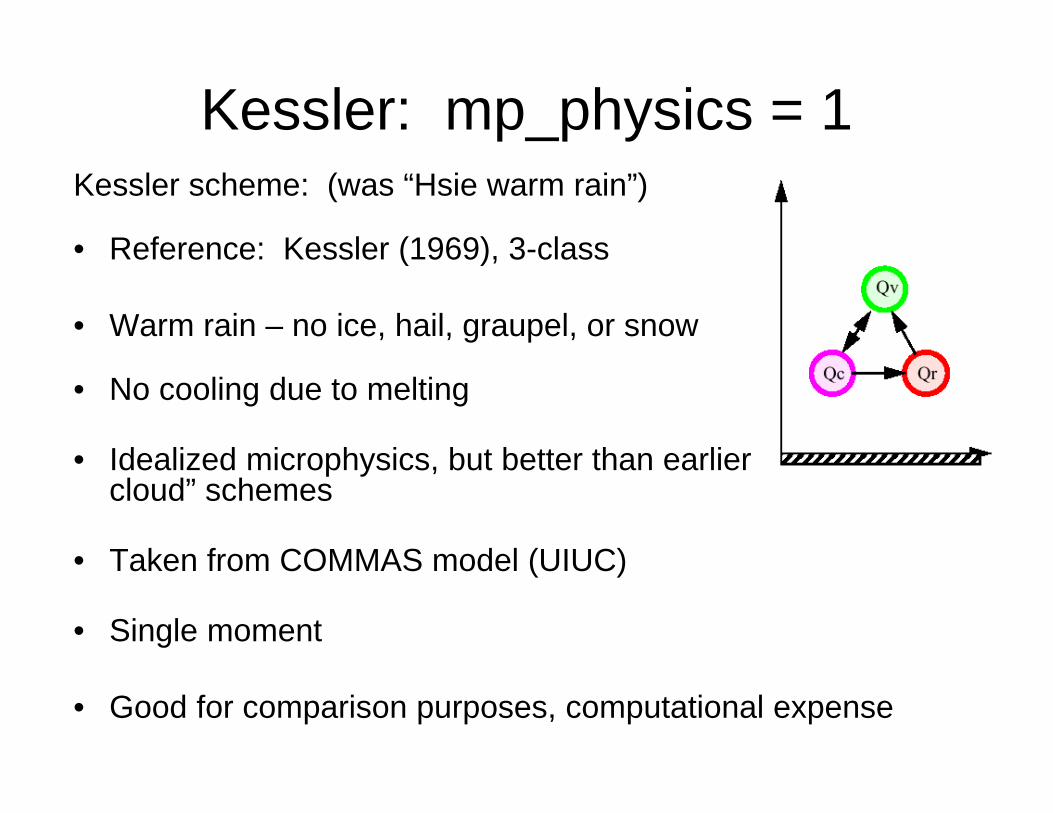
Kessler: mp_physics = 1Kessler scheme: (was “Hsie warm rain”)

• Reference: Kessler (1969), 3-class

• Warm rain – no ice, hail, graupel, or snow

• No cooling due to melting

• Idealized microphysics, but better than earlier “inferred cloud” schemes

• Taken from COMMAS model (UIUC)

• Single moment

• Good for comparison purposes, computational expense

Kessler

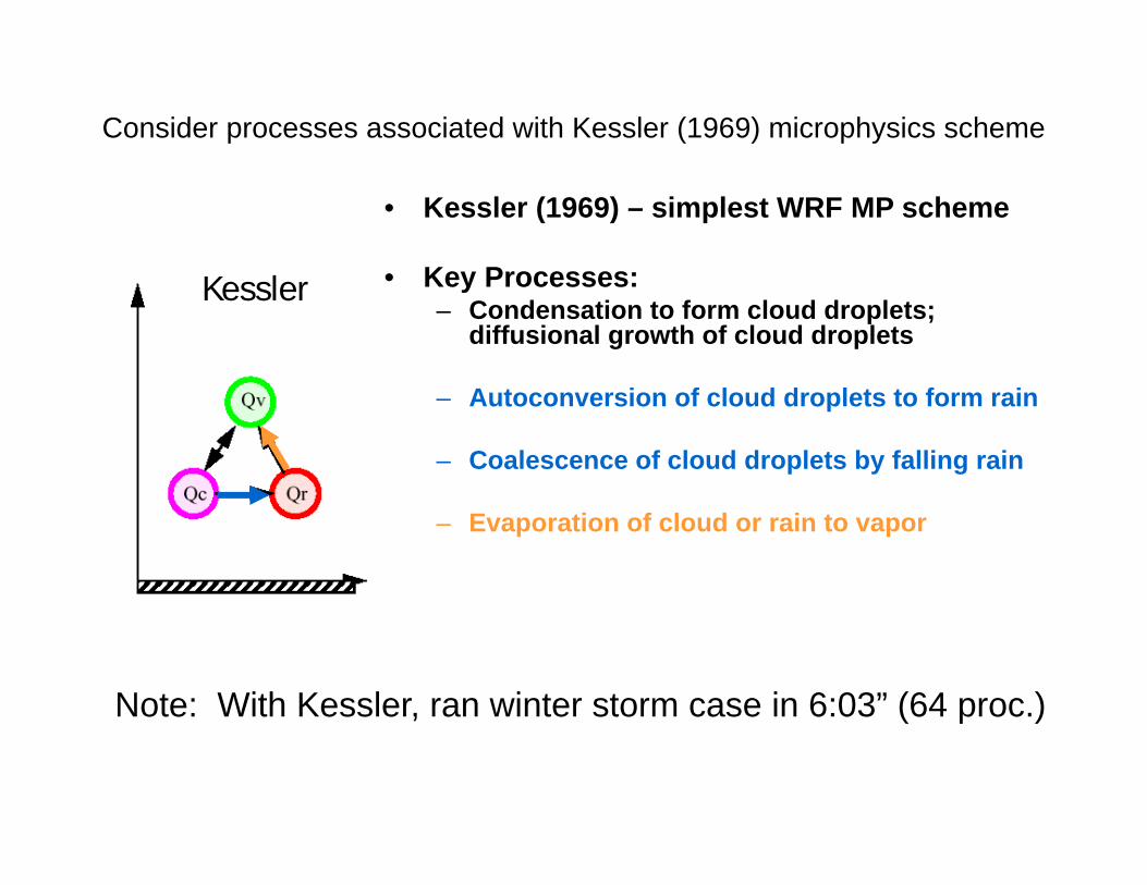
Consider processes associated with Kessler (1969) microphysics scheme

• Kessler (1969) – simplest WRF MP scheme

• Key Processes:– Condensation to form cloud droplets;

diffusional growth of cloud droplets

– Autoconversion of cloud droplets to form rain

– Coalescence of cloud droplets by falling rain

– Evaporation of cloud or rain to vapor

Note: With Kessler, ran winter storm case in 6:03” (64 proc.)

Consider physical processes associated with Kessler (1969) microphysics scheme

Qcloud – cloud liquid water mixing

ratio

Qrain – rain water mixing ratio

Qvapor – Water vapor mixing ratio

Evaporation/ condensation

Autoconversion / coalescence

Evaporation

Sedimentation

Lin: mp_physics = 2“Purdue Lin” scheme, a.k.a. Goddard mixed phase – ahead of its time

References: Lin, Farley, and Orville (1983), Rutledge and Hobbs (1984), Chen and Sun (2002)

• 6-class microphysics including graupel

• Includes ice sedimentation, but single moment, so limitations

• Excessive ice in cloud anvil cirrus, radiative feedbacks

• “Graupel happy” due to lenient definition

• WRF version from Purdue cloud model

• Originally used for high-Plains thunderstorm simulation

• “In this study, we shall use the term “hail” rather loosely to represent high-density graupel, ice pellets, frozen rain, and hailstones” – p. 1067

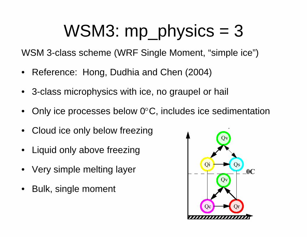
WSM3: mp_physics = 3WSM 3-class scheme (WRF Single Moment, “simple ice”)

• Reference: Hong, Dudhia and Chen (2004)

• 3-class microphysics with ice, no graupel or hail

• Only ice processes below 0C, includes ice sedimentation

• Cloud ice only below freezing

• Liquid only above freezing

• Very simple melting layer

• Bulk, single moment

WSM5: mp_physics = 4WSM 5-class scheme• Also from Hong, Dudhia and Chen (2004)

• Replaces previous NCEP5 scheme

• 5-class microphysics with ice, still no graupel or hail

• Includes supercooled water and snow melt

• Ice sedimentation

• Similar to WSM3, except more completewith Bergeron process, realistic mixed-phase

Adequate for coarse grid spacing, parameterized convection, stable atmosphere

mp_physics=5Ferrier (current NAM) scheme• Designed for computational efficiency

– Advection of total condensate– Cloud water, rain, & ice (cloud ice, snow/graupel)

from storage arrays – assumes fractions of water & ice within the column are fixed during advection

• Has mixed-phase processes to -30C

• May be challenged for proper advection of hydrometeors

• Introduces ice at too warm a temperature?• Tunable parameters, very efficient

Ferrier

Qi/Qs/Qg

Qv

Qc

Qr

Ferrier scheme (cont.)• Ferrier Scheme is in operational NAM model

• Four classes of hydrometeors: • Suspended cloud liquid water droplets • Rain • Large ice (includes snow, graupel, sleet, etc.) • Small ice (generally suspended cloud ice, evaporates quickly in air

subsaturated with respect to ice)

• Only has full prediction equations, including advection, for total condensate (sum of all four hydrometeor classes)

• Does separate (diagnose), but not track with advection, total cloud ice (large ice + small ice), rain, and cloud water

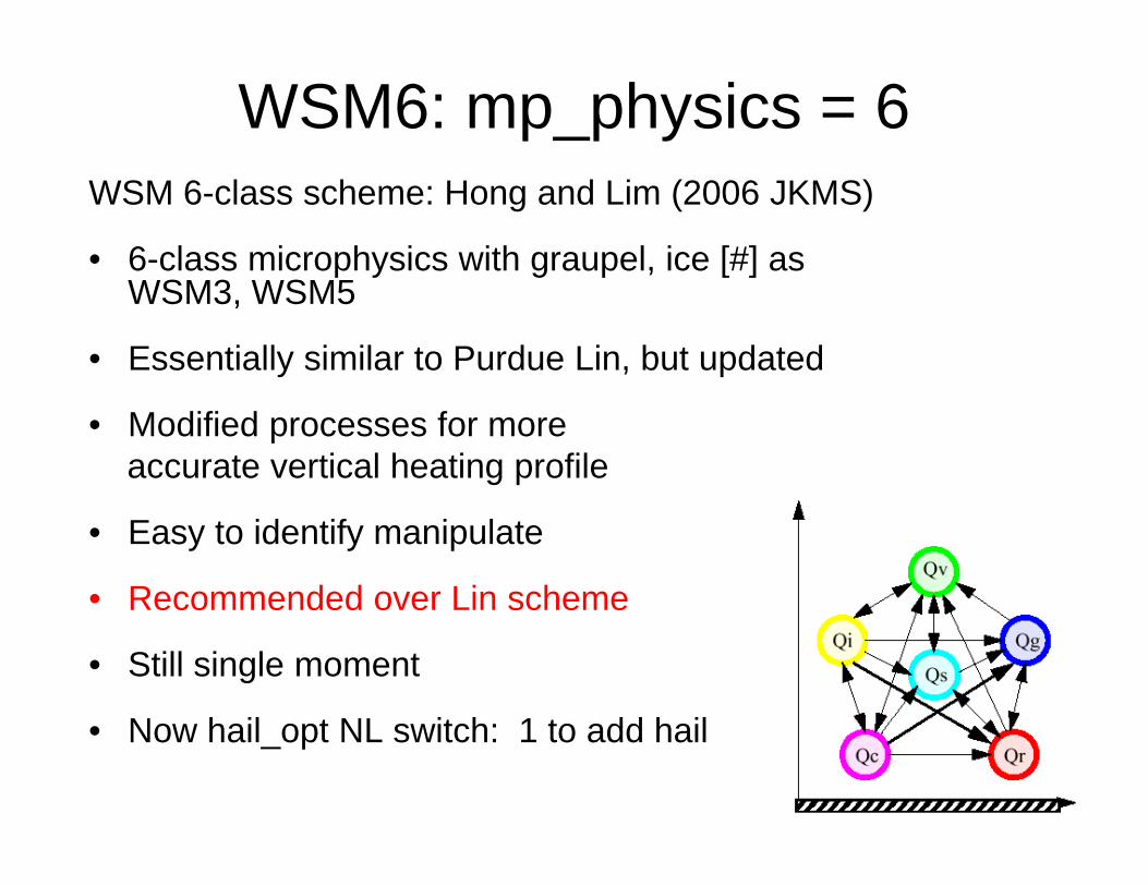
WSM6: mp_physics = 6WSM 6-class scheme: Hong and Lim (2006 JKMS)

• 6-class microphysics with graupel, ice [#] as WSM3, WSM5

• Essentially similar to Purdue Lin, but updated

• Modified processes for more accurate vertical heating profile

• Easy to identify manipulate

• Recommended over Lin scheme

• Still single moment

• Now hail_opt NL switch: 1 to add hail

WSM6 (Hong and Lim 2006)

Goddard: mp_physics = 7Goddard scheme• Reference Tao et al. (1989 MWR - Note)

• 6-class microphysics with graupel

• Similar to Lin, but more hail options – use – gsfcgce_hail: 0 for graupel, 1 for hail – gsfcgce_2ice: 0 for all, 1 for ice and snow, 2 for ice + graupel (?)

• Still single moment

• I have limited experience with it…

• Proven “reasonably accurate” for tropical events, midlatitude convection

Thompson: mp_physics = 8Thompson graupel scheme:

– Reference: Thompson et al. (2004, MWR, updated Thompson et al. 2008)

– Newer version of Reisner2 scheme (MM5)

– 6-class microphysics with graupel

– Double moment, 5 class (now rain also)

– Sophisticated scheme, but computationally affordable

– Two implementations in WRF, 1st had problems, was only 2x Mom. for ice

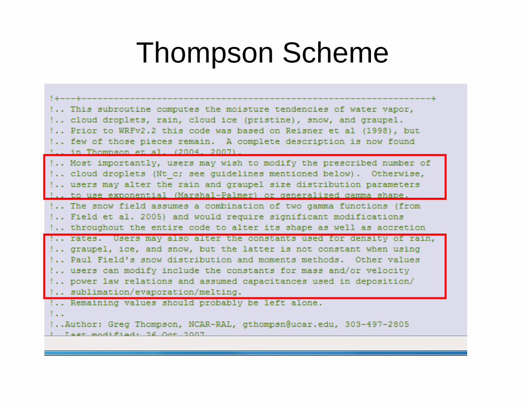
Thompson Scheme

Thompson Scheme

Milbrandt-Yau: mp_physics = 9Milbrandt-Yau scheme:

– Reference: Milbrandt and Yau 2005, series of papers in JAS)

– 7-class microphysics with graupel and hail

– Number concentration also predicted for all 6 water species (fully double moment)!

– Sophisticated process representation but efficient?

Milbrandt-Yau: mp_physics = 9As with Thompson, others, can set air mass type, for single-moment version – [it is switchable (have not tried this)]

Switches to turn on/off some processes

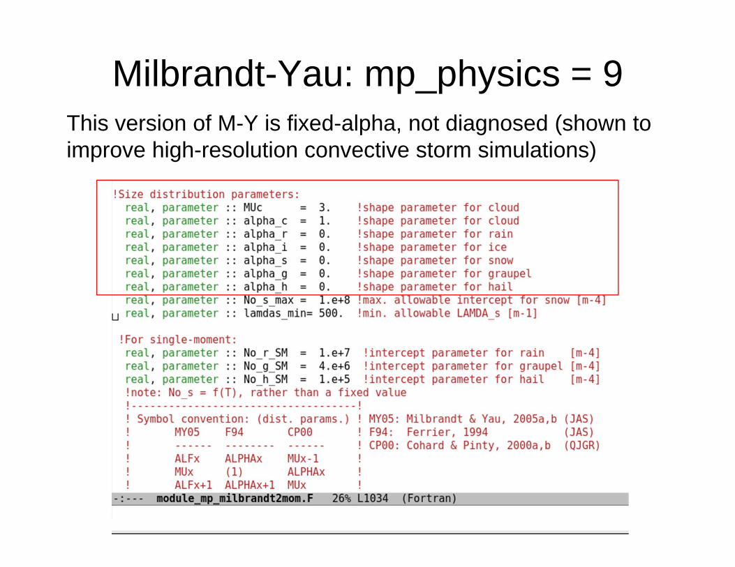
Milbrandt-Yau: mp_physics = 9This version of M-Y is fixed-alpha, not diagnosed (shown to improve high-resolution convective storm simulations)

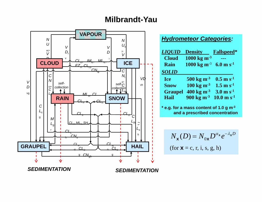
Hydrometeor Categories:

LIQUID Density Fallspeed*Cloud 1000 kg m-3 ---Rain 1000 kg m-3 6.0 m s-1

SOLIDIce 500 kg m-3 0.5 m s-1

Snow 100 kg m-3 1.5 m s-1

Graupel 400 kg m-3 3.0 m s-1

Hail 900 kg m-3 10.0 m s-1

* e.g. for a mass content of 1.0 g m-3

and a prescribed concentration

VDvg

CNig

CLs

h

CLih

CNs

g

CNcr,CLcr

CLc

g

CNgh

CLir-

g

CLir-

g

CLsr-h

CLsr

-g

CLriCLir

CLrsCLsr

MLg

r

MLsr, CL

CLc

h

VDvs

VDvh

CLrh,MLhr,SHhr

VDr

v

CLcs

CLci, IMic, MLic,FZci

RAIN SNOW

GRAUPEL HAIL

NUv

i,VDv

i

NUvc,VDvc

SEDIMENTATIONSEDIMENTATION

self-collection

CNi

s,CLis

self-collection

VAPOUR

ICECLOUD

Milbrandt-Yau

DeDNDN xxxx

0)((for x = c, r, i, s, g, h)

Morrison: mp_physics = 10Morrison Double Moment 6-class:

– Reference: Morrison et al. (2009)

– 6-class microphysics with graupel

– Double moment for cloud water, ice, snow, rain, graupel

– Original papers used for arctic clouds (2005), climate studies, also convection (2009) – radiation interactions considered carefully

– Also hail_opt = 1 to switch

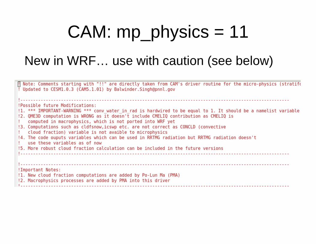
CAM: mp_physics = 11New in WRF… use with caution (see below)

SBU-Lin: mp_physics = 13SUNY Stony Brook (Lin, Colle)

– Reference: Lin and Colle (2011, MWR)

– A 5-class, single moment scheme, no graupel, but a sliding riming scale

– Predicts “precipitating ice”, “riming intensity”

– Continuous spectrum of ice using one variable

– Draws heavily on Purdue-Lin scheme

– Perhaps ideal for winter storms

SBU-Lin: mp_physics = 13Notes from the code:

2) Sedimentation based on Purdue Lin scheme

4) PI size distribution assuming Gamma distribution, but shape parameter mu_s=0 (reduces to exponential) currently

7) The Liu and Daum autoconverion is quite sensitive on Nt_c. For mixed-phase cloud and marine environment, Nt_c of 10 or 20 (E6) is suggested. Default value is 10E.6. Change accordingly for your use.

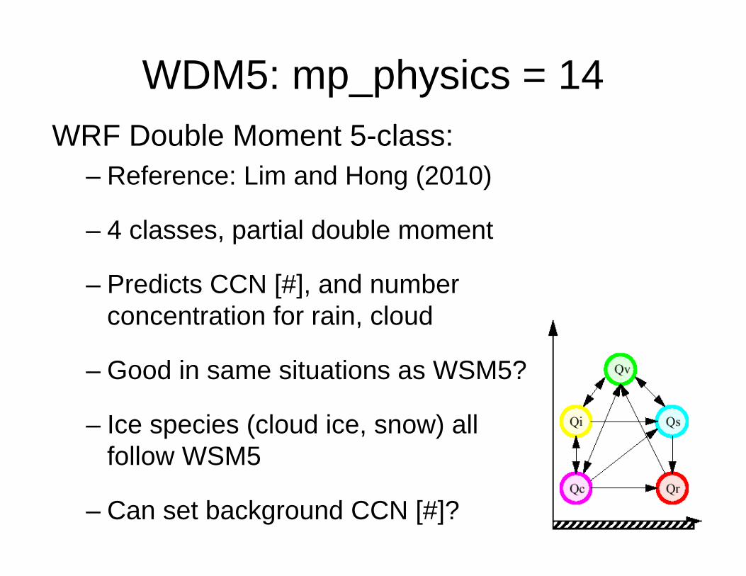
WDM5: mp_physics = 14WRF Double Moment 5-class:

– Reference: Lim and Hong (2010)

– 4 classes, partial double moment

– Predicts CCN [#], and number concentration for rain, cloud

– Good in same situations as WSM5?

– Ice species (cloud ice, snow) all follow WSM5

– Can set background CCN [#]?

WDM6: mp_physics = 16WRF Double Moment 6-class:

– Reference: Hong et al. (2010) and Lim and Hong (2010, MWR)

– 5 classes, double moment for cloud, rain, CCN [#]

– Eliminates biases in WSM6 in published case

– Journal papers compare this to WSM6 for squall line, monsoon

– Utilizes hail_opt, can set CCN?

NSSL: mp_physics = 17, 18NSSL double moment schemes:

– Include both graupel and hail; double moment for 6 classes

– Option 18 predicts CCN, and graupel volume?!

– These have been added to WRF recently (V3.4)

– Additional namelist options available, can set shape parameter, intercept, and density in namelist

– Designed for dx < 2km, maybe idealized best

NSSL: mp_physics = 19,21NSSL single moment schemes:

– Include both graupel and hail

– These have been added to WRF recently (V3.4+) – I’ve very little experience with them

– Additional namelist options available

NSSL: mp_physics = 19,21NSSL schemes:

21, NSSL 1-moment, (6-class), very similar to Gilmore et al. 2004Can set intercepts and particle densities in physics namelist, e.g., nssl_cnorFor NSSL 1-moment schemes, intercept and particle densities can be set for snow, graupel, hail, and rain. For the 1- and 2-moment schemes, the shape parameters for graupel and hail can be set:

nssl_alphah = 0. ! shape parameter for graupelnssl_alphahl = 2. ! shape parameter for hailnssl_cnoh = 4.e5 ! graupel interceptnssl_cnohl = 4.e4 ! hail interceptnssl_cnor = 8.e5 ! rain interceptnssl_cnos = 3.e6 ! snow interceptnssl_rho_qh = 500. ! graupel densitynssl_rho_qhl = 900. ! hail densitynssl_rho_qs = 100. ! snow density

Thompson Aerosol: mp_physics = 28

Aerosol aware, discussed in Thompson and Eidhammer (2014, JAS)

Can utilize CCN climatology (or eventually analysis) for initial conditions

Nate Farrington thesis results – for stratus dissipation

Also excellent interactions with RRTMG radiation scheme (missing for other choices)

Stratus Dissipation: Bottom‐Up Erosion

Morning Afternoon

LCL

LCL

Solar radiation warms PBLLCL raised in response

Stratus Dissipation: Bottom‐Up Erosion

Morning Afternoon

LCLLCL

Larger number concentrationLess solar warming of PBLIncreased cloud lifetime

Stratus Dissipation: Bottom‐Up Erosion

Can a numerical model such as WRF accurately represent this type of cloud‐radiation interaction?  (Twomey, cloud‐lifetime effects)

If cloud‐droplet number concentration increases, should see reduced solar flux at surface for a given amount of cloud (at a certain time of day)

Testable hypothesis:  Plot surface solar flux as function of cloud liquid water content for different experiments

WRF Single‐Column Model Tests

Thompson, RRTMG, nt_c set to 10000

Thompson, RRTMG, nt_c set to 1000

Thompson, RRTMG, nt_c set to 100 (default)

58 W/m2 230 W/m2185 W/m2

GOES 15 Visible satellite17 UTC 18 July 2013

YSU (default and aerosol) + MYJ (default) cloud water with topography, hour 29 (17Z)

17 UTC 18 July 20135x10‐6 kg/kg isosurfaces

YSU (default and aerosol) + MYJ (default) cloud water with topography, hour 29 (17Z)

17 UTC 18 July 20135x10‐6 kg/kg isosurfaces

YSU (default and aerosol) + MYJ (default) cloud water with topography, hour 29 (17Z)

17 UTC 18 July 20135x10‐6 kg/kg isosurfaces

YSU (default and aerosol) + MYJ (default) cloud water with topography, hour 29 (17Z)

17 UTC 18 July 20135x10‐6 kg/kg isosurfaces

HUJI fast: mp_physics = 30New in WRF, BIN scheme from Hebrew

University of Jerusalem

Fast version (still 8,977 lines of code)

Tried running on 64 processors (winter storm case); crashed after ~ 10 hours run time (due to adaptive time step?)

Wall clock per time step ~ 45 seconds versus 0.14 seconds (Kessler, Ferrier), 0.3 WDM5

How to chose a MP scheme?What are you simulating? What MP processes

could affect it, and what scheme best represents those processes?

Is computational cost worth it?

More complex MP schemes may not be compatible with other parameterization schemes (e.g., radiation) which have been developed and tuned to work with simpler schemes (- Morrison workshop presentation)

Performance for winter storm run

0.1

1

10

100

Kessler Fast Bin HUJI Milbrandt‐Yau WDM5 WSM6 (hail opt)

Damage exceeded $2B USD (Durkee et al. 2012)

3-day precipitation exceeded 250 mm over substantial area

Impressive low-level jet, tropical moisture plume, persistence

Case 3: 1-4 May 2010 Tennessee Flood

3-Day total radar-derived rainfall (mm)Maximum: 523 mm

>250 mm

Moore et al. (2011)

1-4 May 2010, TN flooding (Boston.com)

Boston.com

Boston.com

$2.3B in damages estimated, 31 fatalities (Wikipedia)

Boston.com

Radar-derived precipitation total for event: Nashville NWS Radar

Flood Event SimulationGFS analyses for initial, lateral boundary conditions (1.0°)

Initialize 00 UTC 30 April, run 96 h to 00 UTC 4 May 2010

54/18/6/(2) km grid spacing, 1-way nesting

Parameterized convection (BMJ & KF) outer 2 domains, explicit inner

- WSM6 microphysics- YSU PBL, surface layer- NOAH LSM

6 km

18 km

54 km

Precipitable Water (shaded), Reflectivity (black contours)

1-3 May 2010 Tennessee Flooding Event

18-km WRF domain, WSM6, KF CP

Observed Radar, 00Z 5/1-23Z 5/3

Control Simulation

Control simulation: 6 km grid, without CP?

WRF 6-km control simulationObserved Radar, 00Z 5/1-23Z 5/3

Observed radar (left), 2-km domain (Explicit, WSM6)

Domain Comparison, 12 hours

2 km 6 km

18 km

Q2 radar estimate vs. 18-km WRF domain, 72-h total

Q2 radar estimate vs. 6-km WRF domain, 72-h total

Q2 radar estimate vs. 2-km WRF domain, 72-h total

Nate’s MP Assignment: Thompson with RRTMG

Exp - Ctrl

Experiment:

• Tennessee flood event

• CDNC from 100 to 1000 cm-3

Results• Precipitation displaced

north and west of ctrl

• Synoptic precipitation field displaced northward

Ctrl (CDNC 100 cm-1) Exp (CDNC 1000 cm-1)

Results: Albedo (SWDOWN)

Results• The density of the entire cloud shield increased in Exp

• Much less sw radiation reached the surface in Exp• Much more nucleation took place, increasing total droplet SA

Increasing the CDNC of the Thompson MP scheme from 100 cm-3 to 1000 cm-3 was shown to: Displace (in some instances enhance) precipitation downwind Increased the amount of time (and therefore distance) each cloud took

to produce precipitation With more time, more lift, increased LW Path, downstream precip

maxima were observed

Increase cloud nucleation/density (albedo) Much less SWDOWN was observed in Exp versus Ctrl Difference field showed couplets of upwind decrease (increase) and

downwind increase (decrease) in cloud albedo (SWDOWN)

NOTE: Due to my own inability to correctly plot vertical latent heating profiles, I

could not test the latent heating portion of my hypothesis

Conclusions

THE EFFECT OF CHANGING THEINITIAL CLOUD DROPLETCONCENTRATION ON PRECIPITATIONTim GlotfeltyMEA 793, spring 2011

INTRODUCTION

Aerosols impact the environment: One aspect is aerosol indirect effect Several processes are lumped into “indirect effect”,

most well known is the impact of increased aerosols on cloud condensation nucleus distribution

Here, indirect effect of aerosols on precipitation was modeled by changing initial CCN concentration from 100 cm-3 to 1000 cm-3 in WDM6 microphysics scheme for the Tennessee Flooding Case May 1st-4th 2010

HYPOTHESIS

Increasing number of CCN in should result in an overall decrease in precipitation during the event.

More CCN will distribute water vapor over a larger number of smaller drops.

This will decrease ability of drops to grow large enough to fall as rain, thus resulting in lower accumulated rainfall.

PRECIPITATION COMPARISON

00Z May 4th

Control Increased CCN

mm

PRECIPITATION DIFFERENCE

The precipitation appears to have shifted slightly from its original location (As evidenced by the couplet banding).

There are large areas of decreases and smaller areas of increases of roughly the same amount (100-150 mm)

SUMMARY AND CONCLUSION

Increased CCN led to a decrease in the maximum amount of accumulated precipitation by 22 mm.

The increased CCN also resulted in some hot spots of increased precipitation, shifts in cell location

This most likely results from the predicted CCN concentration. The indirect effect is not a linear process. CCN are beneficial

to precipitation until the concentration becomes too large. So in the areas where precipitation increased the increased CCN were most likely in the regime where they helped increase rain formation and the areas that saw decreases were probably in the other. [Also, consider strength of ascent]

Implies that more CCN could cause flooding damage from an event like this to be more localized.

Which MP scheme is best for you?

Discussion

5 minutes: small group5 minutes: discuss in classIdentify group spokesperson

Considerations:

• What phenomena/processes must you forecast/represent?• What grid length are you using?• How much computational expense are you willing to

incur?