© 2016 IEEE. Personal use of this material is permitted. Permission from IEEE must be obtained for all other uses, in any current or future media, including reprinting/republishing this material for advertising or promotional purposes, creating new collective works, for resale or redistribution to servers or lists, or reuse of any copyrighted component of this work in other works.

IEEE ROBOTICS AND AUTOMATION LETTERS. PREPRINT VERSION. ACCEPTED NOVEMBER, 2015 1

Viewpoint Evaluation for Online 3DActive Object Classification

Timothy Patten1, Michael Zillich2, Robert Fitch1, Markus Vincze2 and Salah Sukkarieh1

Abstract—We present an end-to-end method for active objectclassification in cluttered scenes from RGB-D data. Our algo-rithms predict the quality of future viewpoints in the form ofentropy using both class and pose. Occlusions are explicitlymodelled in predicting the visible regions of objects, whichmodulates the corresponding discriminatory value of a givenview. We implement a one-step greedy planner and demonstrateour method online using a mobile robot. We also analyse theperformance of our method compared to similar strategies insimulated execution using the Willow Garage dataset. Resultsshow that our active method usefully reduces the number of viewsrequired to accurately classify objects in clutter as compared totraditional passive perception.

Index Terms—Object detection, segmentation, categorization;Semantic scene understanding; RGB-D perception

I. INTRODUCTION

ACTIVE perception seeks to control the acquisition ofsensor data in order to improve the performance of

perception algorithms. Although certain perception tasks suchas searching [1] and tracking [2] are routinely cast as activeinformation maximisation problems, object classification istraditionally studied as a passive perception problem wheredata are collected during robot navigation and fed into aperception pipeline. We wish to improve the performance ofobject classification algorithms, particularly in cluttered andoccluded environments, by taking an active approach.

Object classification is a key component of many indoorand outdoor robot systems, and helps to enable many othertasks such as grasping, manipulation, and human-robot inter-action. In this work we are directly motivated by domesticscenarios such as tidying a messy room, where static objectslie tangled on the floor [3]. Object classification is necessaryfor identifying and grasping objects, and the robot must alsonavigate through clutter while performing its task. A passiveperception strategy can be equivalent to choosing viewpoints

Manuscript received: September 1, 2015; Revised November 13, 2015;Accepted November 22, 2015.

This paper was recommended for publication by Editor Tamim Asfour uponevaluation of the Associate Editor and Reviewers’ comments.

This research is supported in part by the Australian Centre for FieldRobotics; the New South Wales State Government; the Australian ResearchCouncil’s Discovery Projects funding scheme (project number DP140104203);and the European Community, Seventh Framework Programme (FP7/2007-2013), under grant agreement No. 610532, SQUIRREL.

1T. Patten, R. Fitch and S. Sukkarieh are with the Australian Centrefor Field Robotics, The University of Sydney, Australia {t.patten,r.fitch, s.sukkarieh}@acfr.usyd.edu.au

2M. Zillich and M. Vincze are with the Vision4Robotics Group at theAutomation and Control Institute, Technical University Vienna, Austria{zillich, vincze}@acin.tuwien.ac.at

Digital Object Identifier xxxxxxxxxxxxxxx

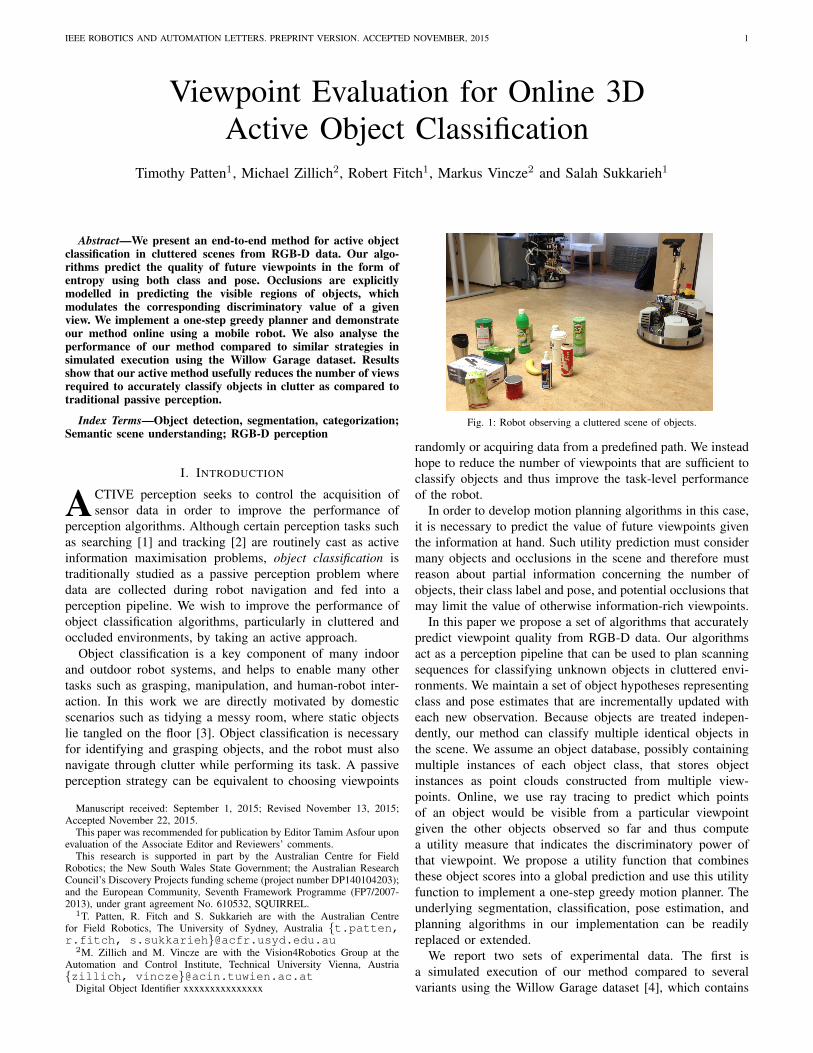
Fig. 1: Robot observing a cluttered scene of objects.

randomly or acquiring data from a predefined path. We insteadhope to reduce the number of viewpoints that are sufficient toclassify objects and thus improve the task-level performanceof the robot.

In order to develop motion planning algorithms in this case,it is necessary to predict the value of future viewpoints giventhe information at hand. Such utility prediction must considermany objects and occlusions in the scene and therefore mustreason about partial information concerning the number ofobjects, their class label and pose, and potential occlusions thatmay limit the value of otherwise information-rich viewpoints.

In this paper we propose a set of algorithms that accuratelypredict viewpoint quality from RGB-D data. Our algorithmsact as a perception pipeline that can be used to plan scanningsequences for classifying unknown objects in cluttered envi-ronments. We maintain a set of object hypotheses representingclass and pose estimates that are incrementally updated witheach new observation. Because objects are treated indepen-dently, our method can classify multiple identical objects inthe scene. We assume an object database, possibly containingmultiple instances of each object class, that stores objectinstances as point clouds constructed from multiple view-points. Online, we use ray tracing to predict which pointsof an object would be visible from a particular viewpointgiven the other objects observed so far and thus computea utility measure that indicates the discriminatory power ofthat viewpoint. We propose a utility function that combinesthese object scores into a global prediction and use this utilityfunction to implement a one-step greedy motion planner. Theunderlying segmentation, classification, pose estimation, andplanning algorithms in our implementation can be readilyreplaced or extended.

We report two sets of experimental data. The first isa simulated execution of our method compared to severalvariants using the Willow Garage dataset [4], which contains

2 IEEE ROBOTICS AND AUTOMATION LETTERS. PREPRINT VERSION. ACCEPTED NOVEMBER, 2015

RGB-D images of occluded objects. The second was collectedby executing our method online using the mobile robot andrepresentative setup shown in Fig. 1. Compared to passiveperception, our method reduced the number of views requiredfor classification by 36% in the Willow Garage dataset anddemonstrated a similar trend in the online validation.

The contribution of this work is an end-to-end method foractive object classification with multiple occluded objects fromRGB-D data. Our method is task-oriented in the sense that it isdesigned to quickly gather information about many objects si-multaneously as opposed to individually. The technical noveltylies in our approach for modulating predictions of viewpointutility learned offline with online prediction of occlusionsand a utility function for planning that jointly considers allobjects and possible states. The benefit of our approach isdemonstrated through experiments that show a reduction in thenumber of views required for scene understanding as comparedto similar methods. Source code used in our experiments isavailable online: https://github.com/squirrel-project.

II. RELATED WORK

Research in active perception has a long history in roboticsand most recently is motivated in part by the now commonavailability of inexpensive RGB-D sensors. Closely relatedwork by Wu et al. [5] focuses on a sensor-object modelfrom RGB-D data that characterises viewpoint and visibilityfor predicted feature matching. Like our method, ray tracingthrough an occupancy grid is used to “filter” out features thatwill be occluded. The main difference, however, is that we donot predict which features will be seen but instead use a learntmeasure of entropy to quantify the quality of a viewpoint andmodulate the expected benefit by the predicted occlusions. Ourwork also differs in that it exploits the probabilistic outputof our classifier to reason about all possible measurementswith their uncertainties, rather than only assuming a single(most likely) class for each object. Lastly, we combine thepredicted utility of each object, with their uncertainties, in ajoint objective function such that the planner maximises thetotal information.

Historically, active perception has mainly been studiedwithin the computer vision community. A good survey can befound in Chen et al. [6]. For classification, a common approachis to formulate the task as a state estimation problem and solveit with information-theoretic metrics in a sequential recog-nition process [7], [8], [9]. Because evaluating differentialentropy or mutual information is intractable in this context dueto the lack of closed form solutions, approximations relying onanalytical bounds [7] or Monte Carlo evaluation [8] are oftenused. Recent work considers choice of classifier, in additionto viewpoint, in a sequential decision-making framework [10].Other work explores robust active object detection [11] andactive object recognition with environment interaction [12].These examples provide end-to-end frameworks, but onlyconsider single objects and do not account for occlusions whenplanning.

An alternative approach is to formulate the problem asa partially observable Markov Decision Process (POMDP).

Approaches to maintain tractable solutions include employingan upper bound on the value function [13] and point-basedapproximation algorithms [14]. These methods are shown toimprove recognition performance in terms of the number ofviews and the distance of the travelled path. Our methodalso represents object states probabilistically, but gains effi-ciency in a different way. We model occlusions explicitly tomodulate offline viewpoint utility measurements. The methodsin [13] and [14] include occlusion as part of the belief state,which increases the size of the problem.

The general problem of passive object classification isimportant in robotics and computer vision. For RGB-D data,methods exist for recognising many instances from a varietyof classes [15]. Work addressing the multi-view case [16],[17] has shown that merging data from different views leadsto improved results, but also highlights the importance ofviewpoint selection. From a theoretical perspective, [18] pro-vides a mathematical description of the tradeoff betweenrecognition and planning, which serves as a justification foractive viewpoint selection as we explore here.

III. PROBLEM FORMULATION

The aim of the active classification problem is for a robot todetermine the class and pose of static objects in an unknownenvironment. The robot processes point cloud observationscaptured with an onboard sensor and selects the next locationto make an observation.

At stage k, a robot has a belief Bk about object states, wherea belief bnk ∈ Bk = {b1k, b2k, ..., b

Nk

k } is maintained for eachobject n ∈ Nk = {1, 2, ..., Nk}. Each belief consists of a classestimate and corresponding pose estimate. The class of an ob-ject is represented by the variable x ∈ X = {x1, x2, ..., xM},where X is the known set of hand-labelled object classes ofsize M . Pose estimates Qn,x

k ∈ Qnk for each class define anaffine transformation of a model to the environment coordinatesystem φ.

From location yk, the robot makes a point cloud observationZk and stores it in a global 3D occupancy grid G. The obser-vation is partitioned into subsets znk ∈ Zk where each subsetpertains to an object. The set of observations of object n upto stage k is denoted by zn1:k = {zn1 , zn2 , ..., znk} and the stateof the object is expressed by the categorical conditional prob-ability distribution pnk (x|zn1:k), where

∑x∈X p

nk (x|zn1:k) = 1

and pnk (x|zn1:k) ≥ 0. Thus the belief of object n is representedby bnk = {pnk (x|zn1:k),Qnk}.

Observing object n from a candidate location y′k+1 ∈ Ykis quantified by the utility value u(y′k+1, b

nk ). Objects are

assumed to be independent such that the total utility functionis the summation of the utilities,

U(y′k+1,Bk) =1

Nk

∑n∈Nk

wnu(y′k+1, bnk ), (1)

where wn is a weighting factor for object n. This weightingfactor will be discussed further in Sec. V.

The set of candidate viewpoints is Yk = Y0\y1:k, whereY0 is the initial set of available locations and y1:k ={y1,y2, ...,yk} is the history of visited locations. The nextlocation is chosen as the one which yields the largest utility.

PATTEN et al.: VIEWPOINT EVALUATION FOR ONLINE 3D ACTIVE OBJECT CLASSIFICATION 3

Planning NavigationObservationProcessing

nextlocation

likelihoodUpdate priorbeliefposteriorbeliefinitialbelief

TrainingDatapointcloud

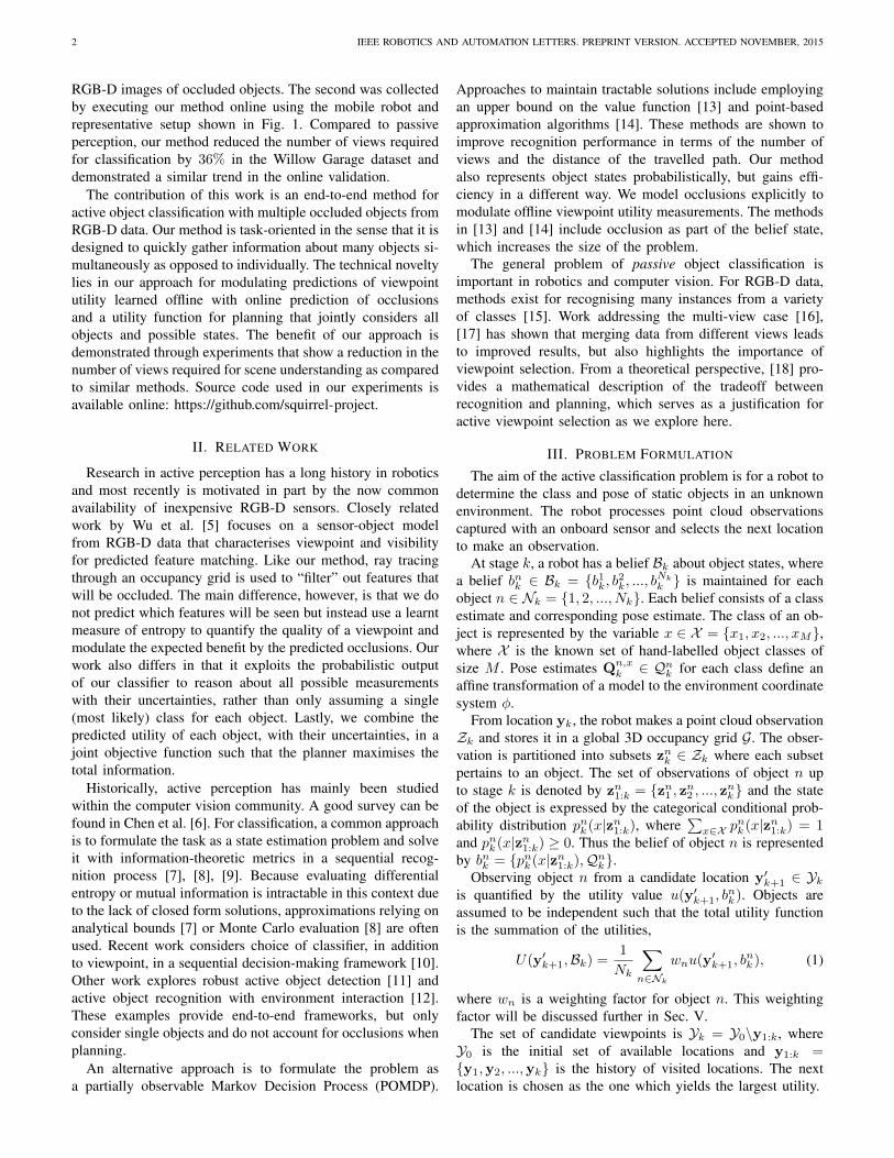
Fig. 2: Overview of the system components.

The active classification problem is defined as follows.Given observations Z1:k = {Z1,Z2, ...,Zk} made from vis-ited locations y1:k and the current belief Bk at stage k, choosethe next location yk+1 from the set of available locations Ykby maximising the utility function

y∗k+1 = arg maxy′k+1∈Yk

U(y′k+1,Bk). (2)

IV. SYSTEM OVERVIEW

An overview of our system is illustrated in Fig. 2. Ateach stage, a planning module uses the current belief andtraining data to determine the next location to make anobservation. The target location is passed to a navigationmodule which drives the robot to the desired goal. At thislocation, the robot makes an observation of the world, whichis input to a processing module to determine an intermediatebelief. This belief is combined with the prior belief in theupdate module to generate a posterior belief that contains allthe information from past observations. Finally, the processrepeats by planning the next observation with the new belief.

V. VIEWPOINT EVALUATION FOR PLANNING

This section describes the planning and navigation modulesof the system. These modules comprise methods for assessingviewpoint quality offline, predicting occlusions online, defin-ing a global utility function and selecting (and navigatingto) future viewpoints, which are integral to solve the overallobjective function (2).

A. Offline Viewpoint Quality

An offline training phase determines a mapping of scalarutility values to viewpoints with respect to an object model.During training, model instances are observed from locationson a 3D view sphere. The quality of each viewpoint isdetermined by the Shannon entropy of the class probabilitydistribution that is generated from classifying the acquiredpoint cloud. (Classification is explained later in Sec. VII-B.)

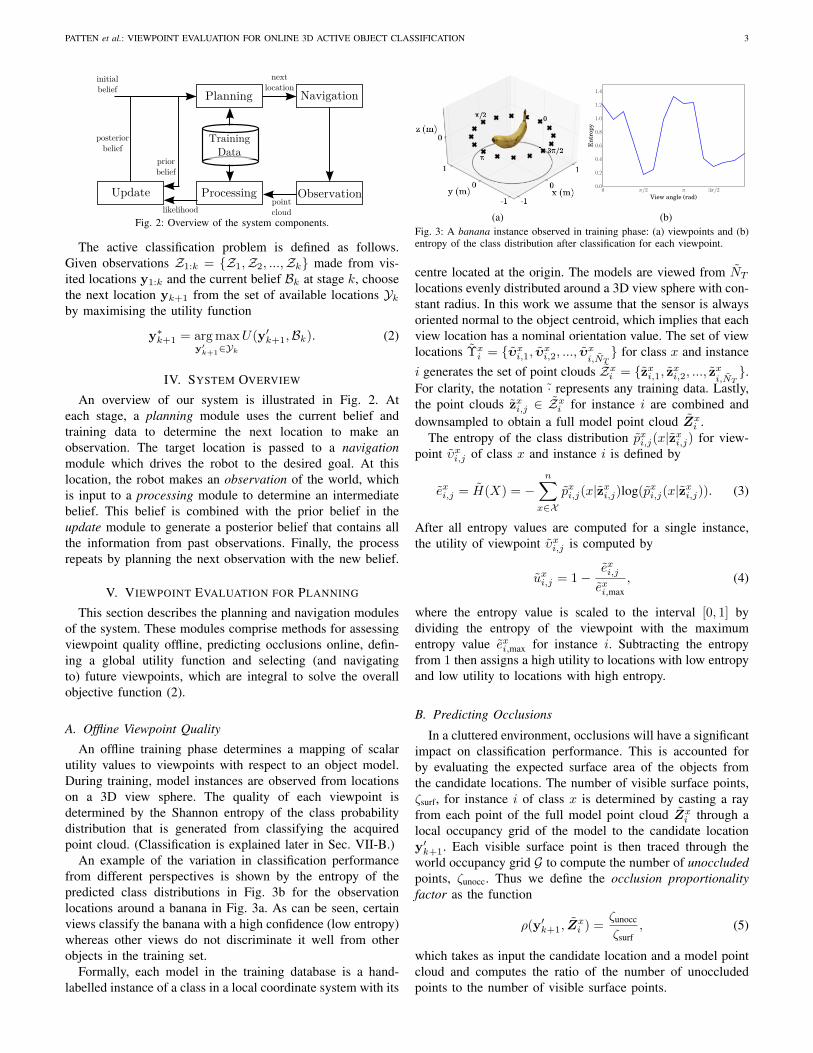
An example of the variation in classification performancefrom different perspectives is shown by the entropy of thepredicted class distributions in Fig. 3b for the observationlocations around a banana in Fig. 3a. As can be seen, certainviews classify the banana with a high confidence (low entropy)whereas other views do not discriminate it well from otherobjects in the training set.

Formally, each model in the training database is a hand-labelled instance of a class in a local coordinate system with its

(a)

0 π/2 π 3π/2

View angle (rad)

0.0

0.2

0.4

0.6

0.8

1.0

1.2

1.4

Ent

ropy

(b)Fig. 3: A banana instance observed in training phase: (a) viewpoints and (b)entropy of the class distribution after classification for each viewpoint.

centre located at the origin. The models are viewed from NTlocations evenly distributed around a 3D view sphere with con-stant radius. In this work we assume that the sensor is alwaysoriented normal to the object centroid, which implies that eachview location has a nominal orientation value. The set of viewlocations Υx

i = {υxi,1, υxi,2, ..., υxi,NT} for class x and instance

i generates the set of point clouds Zxi = {zxi,1, zxi,2, ..., zxi,NT}.

For clarity, the notation · represents any training data. Lastly,the point clouds zxi,j ∈ Zxi for instance i are combined anddownsampled to obtain a full model point cloud Zxi .

The entropy of the class distribution pxi,j(x|zxi,j) for view-point υxi,j of class x and instance i is defined by

exi,j = H(X) = −n∑

x∈Xpxi,j(x|zxi,j)log(pxi,j(x|zxi,j)). (3)

After all entropy values are computed for a single instance,the utility of viewpoint υxi,j is computed by

uxi,j = 1−exi,jexi,max

, (4)

where the entropy value is scaled to the interval [0, 1] bydividing the entropy of the viewpoint with the maximumentropy value exi,max for instance i. Subtracting the entropyfrom 1 then assigns a high utility to locations with low entropyand low utility to locations with high entropy.

B. Predicting Occlusions

In a cluttered environment, occlusions will have a significantimpact on classification performance. This is accounted forby evaluating the expected surface area of the objects fromthe candidate locations. The number of visible surface points,ζsurf, for instance i of class x is determined by casting a rayfrom each point of the full model point cloud Zxi through alocal occupancy grid of the model to the candidate locationy′k+1. Each visible surface point is then traced through theworld occupancy grid G to compute the number of unoccludedpoints, ζunocc. Thus we define the occlusion proportionalityfactor as the function

ρ(y′k+1, Zxi ) =

ζunocc

ζsurf, (5)

which takes as input the candidate location and a model pointcloud and computes the ratio of the number of unoccludedpoints to the number of visible surface points.

4 IEEE ROBOTICS AND AUTOMATION LETTERS. PREPRINT VERSION. ACCEPTED NOVEMBER, 2015

C. Global Utility Function

The utility of observing object n from a candidate locationy′k+1 is calculated by

u(y′k+1, bnk ) =

1

M

∑x∈X

[pnk (x|zn1:k)×

ρ(y′k+1, ZxI )

NT

∑j∈NT

uxI,je−d(y′

k+1,τ )/σ], (6)

where d(·, ·) is the Euclidean distance between two locations,τ = Qn,x

k υxI,j is the transformation of the viewpoint intothe map frame and σ is a scalar variance. Note that thesubscript I on the viewpoint υxI,j , the utility value uxI,j , andthe model point cloud ZxI represent the training instance ofclass x that has the strongest belief. The term e−d(y

′k+1,τ)/σ

scales the utility contribution of viewpoint υxI,j by its distancefrom the candidate location, which accounts for both angularand distance error between y′k+1 and τ . This term makesthe reasonable assumption that the utility value is continu-ous between different training viewpoints. More sophisticatedmethods (e.g., Gaussian processes) could be used to model thetrue relationship but this is beyond the scope of this paper.

This function computes the utility of the known viewpoints,weighted by their distance to y′k+1, and weights the contri-bution of each possible class by its probability. The utilityvalues are also modulated by the occlusion proportionalityfactor. Intuitively, if an object is highly occluded from locationy′k+1 then its utility contribution will be very small becauseζunocc � ζsurf. From such an occluded viewpoint, it is ex-pected that the object will not be strongly recognised and theobservation will not be beneficial. If an object is unoccludedthen the utility contribution will approach the training utilityvalue because ζunocc ≈ ζsurf. The occlusion factor is containedwithin the summation over the class distribution such that anocclusion state is computed separately for each class.

We define the object weighting factor wn in (1) by theentropy of the object’s probability distribution, i.e.

wn = H(Xn) = −∑x∈X

pnk (x|zn1:k)log(pnk (x|zn1:k)). (7)

This means that an object which the robot is unsure about(high entropy) will have more influence on the decision thanan object that a robot is more sure about (low entropy).

Substituting (6) and (7) into (1) yields the utility function

U(y′k+1,Bk) =1

Nk

∑n∈Nk

[H(Xn)

M×

∑x∈X

[pnk (x|zn1:k)

ρ(y′k+1,Z

xI )

NT

∑j∈NT

uxI,je−d(y′

k+1,τ)/σ]]. (8)

D. Viewpoint Selection and Navigation

The procedures outlined above determine a utility score fora candidate location y′k+1. Selecting the next best view in-volves computing the utility value for each potential viewpointy′k+1 ∈ Y , then selecting and immediately navigating to theviewpoint which has the highest expected utility. This work

assumes a given set of initial viewpoints Y0 with associatedcollision-free navigation roadmap, and removes each locationyk from the set as they are visited such that Yk = Y0\y1:k. Ateach stage, the remaining unvisited viewpoints are evaluatedto search for the next best view.

VI. FUSING NEW OBSERVATIONS

In this section we present the update module of the system.This module associates observations to objects and updatesclass distributions and pose estimates.

A. Data Association

Each observation is stored in a 3D occupancy grid G.The occupied space of each object n can be computed bydetermining the voxels that correspond to the observationszn1:k−1. The set of voxels for each new segment is comparedto the voxel set of each object in the prior belief Nk−1.A segment is associated to an object if the proportion ofvoxels overlapping those of a prior object is greater than agiven threshold. The proportion is computed as the sum ofthe number of overlapping voxels divided by the total numberof occupied voxels for the segment. Set Nk is maintained byadding new objects for unassociated segments and mergingassociated segments with existing objects as appropriate.

This procedure can become costly because it must performN2V 2 voxel checks where N is the number of hypotheses andV is the number of voxels occupied by an object. We speed upthe process by first comparing the bounding boxes of the objectpoint clouds in the two different sets. Voxel matching is thenonly performed with the objects that pass the quick boundingbox check. This greatly reduces the number of voxel checks.

Note that our association method assumes that objects arestatic and that the localisation and measurement errors aresmall. In our experiments, the errors were not large enough tocause problems, however, for situations with large error, morerobust association methods could be used such as [19].

B. Class Distribution Update

The probability class distribution of object n is updated byapplying Bayes’ rule

pnk (x|zn1:k) = ηpnk−1(x|zn1:k−1)pnk (znk |x), (9)

where pnk−1(x|zn1:k−1) is the prior, pnk (znk |x) is the likelihoodand η is a normalisation constant. The prior for a newobservation segment is the combination of the probabilitydistributions of its associated objects. The previous observa-tions are considered independent, so the probabilities can becomputed by multiplying each element and normalising.

In this work we assume a classifier that can be queriedfor a single observation znk to return a probability distributionover classes pnk (x|znk ). From Bayes’ rule, the output can beexpressed as

pnk (x|znk ) = η0pnk (x|zn0 )pnk (znk |x), (10)

where η0 is a normalisation constant different from η. For asingle point cloud query, the prior contains no observations, i.e.

PATTEN et al.: VIEWPOINT EVALUATION FOR ONLINE 3D ACTIVE OBJECT CLASSIFICATION 5

zn0 = ∅, and assuming a uniform prior, pnk (x|zn0 ) = pnk (x) =uniform, (10) is equivalent to

pnk (x|znk ) = pnk (znk |x), (11)

meaning that the likelihood pnk (znk |x) in (10) uses the outputof a classifier, where observation znk is used as its input.

C. Pose Estimate Update

The planning module requires a pose estimate for eachobject-class pair. In principle, the pose estimate from the latestobservation could be used, but it is likely that poor estimatesare made when objects are only partially observed.

We assume a pose estimator that can output a measureof estimation quality. In our implementation, this measureis provided by the alignment error of the iterative closestpoint (ICP) algorithm [20]. To provide a better pose estimate,Qn,xk−1 (for object n and class x) is replaced if the ICP error

is larger than the ICP error of the new pose estimate fromthe latest observation. The pose estimates of each class areconsidered independent, which means that each estimate canbe replaced irrespective of other estimates. This procedureobtains the new set of poses Qnk for each object n ∈ Nk.

VII. POINT CLOUD PROCESSING

This section describes our implementation of the processingmodule of the system. This module can be implemented usingany perception tools that output a set of partitioned pointclouds with associated class probability distributions and poseestimates.

A. Segmentation

Segmentation is performed using the method in [21]. Thescene is first decomposed into surface patches, fitting planesand Non-Uniform Rational B-splines (NURBS). A series ofperceptual grouping principles is then run to establish pairwiseprobabilities of two surfaces belonging to the same object.These probabilities generate edge weights in a graph of surfacepatches, and a graph cut algorithm is used to optimallypartition the graph to yield object hypotheses. The set of objectsegments is then post-processed to cull background objects(those not lying directly on the ground plane/table top). Thissegmentation method also handles the case of touching orstacked objects; see [21] for more details.

B. Classification

Classification is performed using [22]. The classifier is builtoffline by generating partial point clouds of object modelsin a pre-defined database. The database consists of a largenumber of model instances which are grouped into classes.Partial point clouds are generated from given locations ona 3D view sphere and a global feature descriptor is com-puted for each point cloud. Here, we use the ensemble ofshape functions (ESF) descriptor, which consists of ten 64-bin histograms based on distinct shape functions (distance,angle and area distributions) [23], although any global featuredescriptor could be used. The descriptors for each viewpoint

and instance, along with the class label, are stored in a k-dtree with dimension 640. Online classification of a point cloudproceeds by computing the ESF descriptor and calculating thedistance in the k-d tree to the closest Nc nodes. The numberof nodes for each class are tallied to determine a score, whichis then normalised by dividing by Nc, allowing the output tobe interpreted as a probability.

Note that the object models used for training the classifierare the same as those used for computing the offline utilityvalues. Thus, the predicted utilities are directly related to theclassifier and accurately predict the belief updates.

C. Pose Estimation

The pose estimate for each class x is computed separatelyfrom the segmented point clouds znk , where a pose estimateis an affine transformation matrix of a training model pointcloud into the world coordinate system φ. Each znk is alignedwith training point cloud Zxbest corresponding to the most likelyinstance of class x as follows:(i) Downsampling: The point clouds are downsampled usinga uniform grid to speed up computation.(ii) Initial scaling: The ESF descriptor is scale independent,therefore the training models can be a different size to theobserved objects. Zxbest is expanded or contracted such thatthe dimensions of its minimum bounding box are similar tothe dimensions of the minimum bounding box of znk .(iii) Initial alignment: The training models are viewed in alocal coordinate system with the model centred at the origin.Zxbest is positioned at the origin of φ to bring the point cloudsinto a common reference frame, then translated so that itscentroid has the same coordinate as the centroid of znk .(iv) ICP and scale refinement: The partial point cloud isaligned to the test point cloud using ICP. ICP is seeded from4 different rotations (0, π/2, π, 3π/2) on each axis and thealignment with the smallest ICP error is retained. We alsomake scale refinements with each iteration by performing agrid search over scale. If any new scale has a smaller error, itis maintained for the next iteration.

The modified ICP algorithm that performs scale adjustmentsis necessary to improve upon the initial scale guess and to takeinto account occlusions. As an example, a point cloud from anoccluded view is likely to be smaller than if it were observedwithout any occlusion. The fine scale adjustment will bring thetest point cloud to a size that better represents the observedpoint cloud.

VIII. RESULTS

In this section we present two sets of results. First, wepresent quantitative experiments using the Willow Garagedataset with comparison to related methods. Second, weprovide validation and demonstration with a mobile robotperforming online active object classification using our methodin two different setups and compare its performance withpassive perception.

6 IEEE ROBOTICS AND AUTOMATION LETTERS. PREPRINT VERSION. ACCEPTED NOVEMBER, 2015

A. Willow Garage Dataset

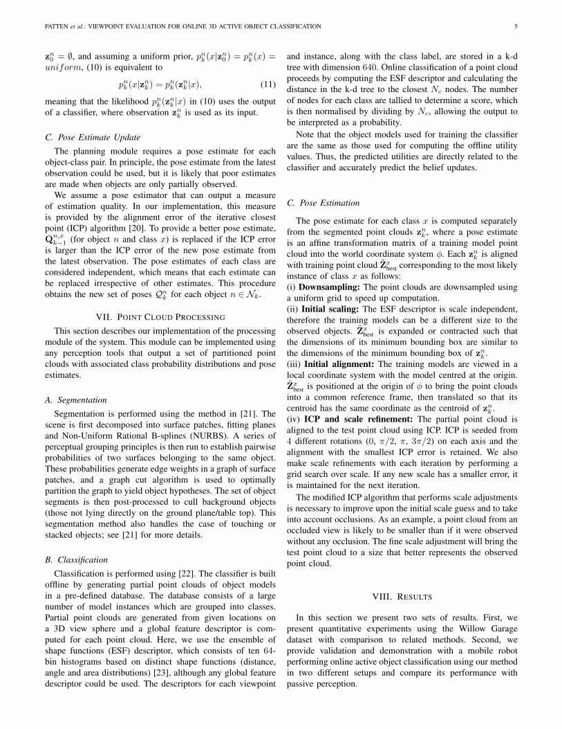
1) Experimental Setup: The Willow Garage dataset consistsof Kinect RGB-D sensor data of household objects on atable top. An example is shown in Fig. 4a. The datasetcomprises 24 scenarios, but we rejected 5 because they containglass objects which could not be detected with the sensor(6, 22, 23, 24) or segmentation failed (16). Each scenariocontains 6 objects viewed from 11−19 different perspectives.For each observation, the viewpoint in the map frame wasextracted so that the behaviour of the robot selecting real worldobservations could be simulated.

The classifier was trained on 15 classes, where each classcomprised 5−20 instances. The viewing radius was set to 2mand each instance was viewed from NT = 20 locations. Weset σ = 0.5m, which is reasonable since locations closer than0.1m to a training viewpoint will contribute approximately80% of its utility value, while locations further than 1m willcontribute less than 15% of their utility values. The number ofnearest neighbours in the k-d tree search was set to 50 and thevoxel overlap threshold for data association was set to 20%.

2) Comparison Methods and Metric: We evaluated theeffectiveness of our proposed utility function by comparingit to a variety of alternatives. The full set of methods were:(UE) Our method using weighted contribution of trainingviewpoint utility and occlusion reasoning.(UP) Using the training viewpoint that has the highest prob-ability of the true class. That is, given the probability vectorpxi,j(x), the utility of training viewpoint υxi,j(x) is quantifiedby its classification performance w.r.t. the true class, i.e.pxi,j(xtrue). The utility values µxi,j in (6) were replaced withpxi,j(xtrue) to compute (8).(E) Our method without occlusion reasoning, so that view-points are only selected by their classification ability.(P) Variant (UP) without occlusion reasoning.(A) Selecting viewpoints which maximise the expected surfacearea. The class weight wn in (1) defined by the entropy of theobject was maintained, but u(y′k+1, h

nk ) was replaced by the

number of expected surface points for object n.(NE) Selecting viewpoints nearest to the training viewpointwith maximum utility for the most uncertain object.(R) Passively selecting views at random.(S) Passively selecting sequential viewpoints on perimeter.

The sequential method (S) is typical of a passive perceptionstrategy that is driven by a navigation goal (drive around aperimeter of the scene). Here, viewpoints were selected inclockwise order. The random strategy (R) is also a usefulcomparison because it avoids any bias induced by the startingview of a sequential strategy.

Each simulation began from the same randomly selectedviewpoint and was terminated at the “knee” of the meanprobability curve, which was determined where the curve didnot increase by more than 0.5% for 4 consecutive observations.The “knee” point with lowest confidence was selected asthe threshold for the comparison. The performance of eachstrategy was measured by the number of views required forthe mean probability curve to reach the confidence threshold.Typical values of the threshold ranged between 70 − 80%,

(a)

UE UP E P A NE R SPlanner

0

2

4

6

8

10

12

14

Mea

nnu

mbe

rof

view

s

6.1 6.4 7.1 7.3 7.68.4

9.3 9.2

(b)Fig. 4: Example comparison of planning strategies for one scenario in WillowGarage dataset: (a) the experimental setup and (b) the histogram of the meannumber of views to reach confidence threshold.

UE UP E P A NE R S

01 4.7 (1.4) 5.1 (1.2) 4.7 (1.4) 5.1 (1.2) 5.8 (1.9) 5.5 (1.9) 5.9 (2.8) 7.7 (3.7)02 4.8 (2.5) 8.4 (5.0) 4.8 (2.0) 6.0 (3.7) 3.9 (1.6) 5.0 (2.2) 5.9 (1.7) 7.8 (4.0)03 4.2 (1.2) 4.6 (1.3) 4.4 (1.1) 4.4 (2.3) 6.0 (2.9) 5.5 (2.6) 6.4 (2.1) 7.6 (3.6)04 5.8 (4.2) 5.3 (2.6) 7.6 (4.3) 10.2 (4.9) 7.3 (4.4) 6.3 (3.7) 6.3 (2.7) 5.9 (4.4)05 6.0 (1.7) 5.5 (1.6) 7.5 (3.1) 6.6 (2.7) 7.5 (2.9) 5.4 (2.3) 5.5 (2.4) 7.8 (4.4)07 5.3 (2.1) 4.7 (1.2) 6.4 (1.6) 6.0 (1.6) 5.8 (2.8) 7.1 (3.4) 5.5 (3.2) 7.2 (6.3)08 6.1 (2.5) 6.4 (3.1) 7.1 (3.1) 7.3 (4.2) 7.6 (3.2) 8.4 (4.0) 9.3 (4.7) 9.2 (5.7)09 5.1 (1.7) 5.6 (3.6) 4.8 (2.2) 4.8 (1.8) 5.5 (2.4) 5.0 (1.3) 5.6 (3.1) 10.5 (5.0)10 4.7 (2.1) 6.5 (4.1) 9.1 (5.5) 7.1 (4.7) 8.0 (5.0) 8.2 (5.5) 10.7 (4.0) 10.8 (4.1)11 3.9 (1.3) 3.9 (1.9) 4.0 (1.8) 4.0 (1.6) 4.2 (2.3) 4.5 (1.7) 4.3 (1.8) 7.8 (2.8)12 9.1 (5.8) 8.0 (5.6) 10.2 (6.2) 10.6 (6.3) 10.0 (6.4) 7.0 (4.6) 9.9 (5.7) 8.6 (3.0)13 5.6 (1.2) 6.5 (1.5) 7.1 (2.0) 6.5 (1.8) 7.4 (1.3) 9.5 (4.1) 9.7 (3.3) 11.6 (5.2)14 3.5 (1.3) 3.1 (0.7) 3.5 (0.8) 3.6 (1.1) 3.3 (0.9) 3.3 (0.9) 5.4 (1.7) 7.6 (5.0)15 8.8 (3.4) 10.3 (5.0) 10.3 (4.4) 10.3 (3.9) 10.5 (4.8) 9.8 (3.9) 9.8 (5.2) 15.4 (1.8)17 2.7 (0.5) 2.7 (0.5) 2.7 (0.5) 2.7 (0.5) 2.7 (0.5) 3.4 (1.6) 4.3 (1.4) 4.5 (1.9)18 8.4 (3.6) 8.2 (4.2) 7.8 (3.7) 8.6 (4.4) 9.0 (3.7) 11.6 (3.5) 8.5 (3.4) 14.9 (0.3)19 7.7 (3.7) 8.1 (4.4) 8.3 (3.5) 8.6 (3.9) 7.6 (3.2) 9.3 (4.1) 11.8 (3.6) 7.5 (4.3)20 4.3 (1.1) 5.5 (1.9) 4.4 (1.3) 5.4 (3.8) 4.5 (1.3) 6.4 (3.7) 11.5 (3.1) 5.7 (3.9)21 3.1 (1.0) 3.7 (2.0) 4.4 (2.1) 4.1 (2.0) 4.0 (1.7) 4.2 (2.2) 4.6 (2.0) 3.6 (1.6)

mn 5.5 (1.9) 5.9 (2.0) 6.3 (2.3) 6.4 (2.4) 6.3 (2.2) 6.6 (2.3) 7.4 (2.6) 8.5 (3.1)

TABLE I: Number of views to reach confidence threshold in the WillowGarage dataset. Rows correspond to dataset scenarios and columns correspondto planning strategies (best planner shown in bold). The last row shows meannumber of views with standard deviations in parentheses.

which is a reasonable level of confidence for occluded data.3) Results Discussion: Average results from 10 simulations

(from 10 different starting locations) are shown in Fig. 4bfor the setup in Fig. 4a. This example shows that all activestrategies recognise the objects faster than the random andsequential strategies. The best performance is achieved by ourplanner (UE), with a 14% improvement compared to whenocclusions are not accounted for (E). The example shows thatselecting viewpoints which maximise surface area (A) tendsto have worse performance than the other utility functions.All active planners which consider all objects simultaneouslyoutperform the method that selects locations nearest to thelowest entropy viewpoint for the most uncertain object (NE).

This procedure was repeated for the other scenarios andresults are presented in Tab. I. In 15 scenarios, minimisingentropy (UE,E) or maximising class probability (UP,P) re-quired the fewest views. In 10 of the scenarios, our utilityfunction (UE) performed best. In the remaining scenarios, thebest performing methods were maximising surface area (A)(2 cases), selecting viewpoints closest to the highest utilitylocation for the most uncertain object (NE) (2 cases), andsequential views (1 case). Random viewpoint selection neverachieved the best performance.

The last row in Tab. I shows mean results. Our methodhas the lowest mean and smallest standard deviation. Incomparison to the same utility function, which uses the classprobability (UP), the performance is on average 7% better.

PATTEN et al.: VIEWPOINT EVALUATION FOR ONLINE 3D ACTIVE OBJECT CLASSIFICATION 7

(a) (b)Fig. 5: Setup 1: (a) side view and (b) top view.

0 1 2 3 4 5 6

Number of views

0.0

0.2

0.4

0.6

0.8

1.0

Mea

npr

obab

ility

ProposedSequentialRandom

(a)

0 1 2 3 4 5 6

Number of views

0.0

0.5

1.0

1.5

2.0

2.5

3.0To

tale

ntro

py

ProposedSequentialRandom

(b)Fig. 6: Comparison of active planner with random and sequential for setup1: (a) mean of the true class probability for each object and (b) total entropyof the object class distributions.

(a) (b)Fig. 7: Setup 2: (a) side view and (b) top view.

0 1 2 3 4 5 6

Number of views

0.0

0.2

0.4

0.6

0.8

1.0

Mea

npr

obab

ility

ProposedSequentialRandom

(a)

0 1 2 3 4 5 6

Number of views

0.0

0.5

1.0

1.5

2.0

2.5

3.0

Tota

lent

ropy

ProposedSequentialRandom

(b)Fig. 8: Comparison of active planner with random and sequential for setup2: (a) mean of the true class probability for each object and (b) total entropyof the object class distributions.

Both these strategies have better performance when accountingfor occlusions, for the case of views with minimum entropythe improvement is 13% while for the case of views withmaximum probability the improvement is 8%.

There is little difference between the two utility functionswhich do not account for occlusions (E,P), and the sameperformance is achieved by maximising surface area (A).This shows that similar performance is achieved using eitherobjective separately, but using them jointly is beneficial.

The worst performing active planner is (NE). This indicatesthat it is advantageous to consider all objects simultaneouslybecause single observations can provide information aboutmultiple objects and their estimates can improve together,which may lead to greater improvement overall.

As expected, all active planners outperform random andsequential. For comparison, our method recognises objectswith nearly 2 and 3 fewer views, an improvement of 26%and 36% respectively. Random outperforms sequential by 1fewer view and has a smaller variance, indicating that randomis an adequate comparison for evaluating active strategies.

B. Hardware Experiments

1) Experimental Platform: Our robot is a Festo Robotinowith custom-mounted ASUS XTion Pro Live RGB-D sensor,shown earlier in Fig. 1. Software is written in C++ using thepoint cloud library [24], octomap [25] and ROS [26].

2) Experimental Setup: The classifier was trained with thesame database of objects and parameters as the previousexperiments. The localisation error was larger, so the voxeloverlap threshold for data association was increased to 40%.

There are two setups, shown in Figs. 5 and 7, that consistof objects on the floor belonging to the classes can, bottleand box in a variety of shapes and sizes. The initial set ofviewpoints was pre-selected as 12 evenly spaced locations ona circle around the objects with radius 2m. A simple roadmapconnects each viewpoint to its neighbours for navigation.

Two hardware experiments (one for each setup) were per-formed with our method and terminated after 6 observations.These observations were sufficient because the class confi-dence did not increase significantly after this point. For com-parison, we performed offline simulations where viewpointswere selected at random or sequentially (clockwise) around ahalf circle. Simulations used the data collected during onlineexperiments combined with pre-collected observations fromthe remaining viewpoints. For each setup, 10 simulations wererun in the random case and 1 in the sequential case. Theinitial viewpoint for both cases was set to coincide with theinitial viewpoints of the online experiments, and likewise, 6observations were made in total.

A comparison of the performance between active and pas-sive planning was done using two metrics. The first was meanprobability, pk = 1

Nk

∑n∈Nk

pnk (xGT), which is the averageprobability of the ground truth class xGT of each object. Thismetric evaluates the accuracy of the classifier at the level ofindividual objects. The second was total entropy, which is thesum of the entropies of each object’s class distribution. Thismetric evaluates the uncertainty of the classifier’s estimate.

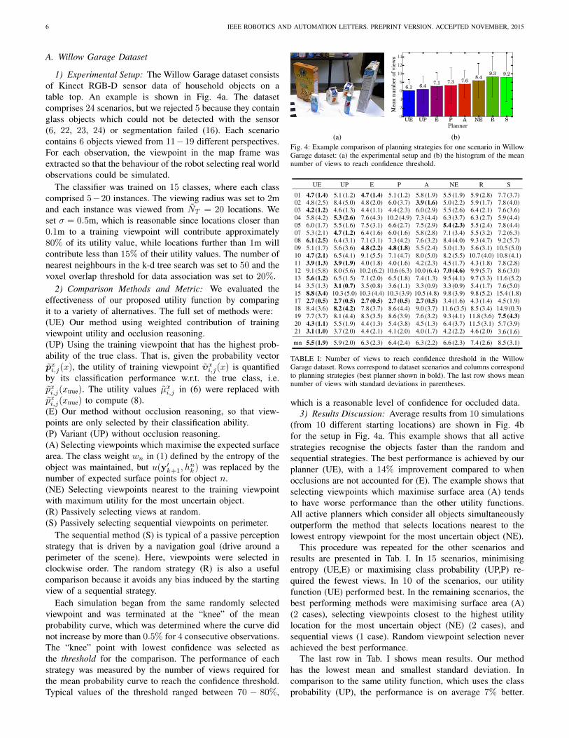
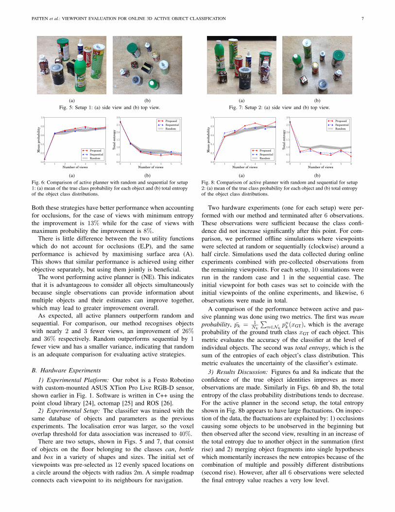
3) Results Discussion: Figures 6a and 8a indicate that theconfidence of the true object identities improves as moreobservations are made. Similarly in Figs. 6b and 8b, the totalentropy of the class probability distributions tends to decrease.For the active planner in the second setup, the total entropyshown in Fig. 8b appears to have large fluctuations. On inspec-tion of the data, the fluctuations are explained by: 1) occlusionscausing some objects to be unobserved in the beginning butthen observed after the second view, resulting in an increase ofthe total entropy due to another object in the summation (firstrise) and 2) merging object fragments into single hypotheseswhich momentarily increases the new entropies because of thecombination of multiple and possibly different distributions(second rise). However, after all 6 observations were selectedthe final entropy value reaches a very low level.

8 IEEE ROBOTICS AND AUTOMATION LETTERS. PREPRINT VERSION. ACCEPTED NOVEMBER, 2015

can bottle banana spraybottle

0.0

0.5

1.0

Pro

babi

lity

Entropy = 0.95

(a)

can bottle banana spraybottle

0.0

0.5

1.0

Pro

babi

lity

Entropy = 0.25

(b)Fig. 9: Selected viewpoint in the online experiment of setup 2, showing theRGB-D observations, the probability values for the 4 top scoring classes andthe entropy of the total distribution for the Stiegel can (red and white) locatedin the centre: (a) viewpoint 2 and (b) viewpoint 3.

In the first setup, we can see that after 3 observations theobject confidence for the active planner reaches a plateau.This level is only reached by the random and sequentialplanners after all 6 views are observed. In the second setup,the sequential and random planners never reach the level ofcertainty of the active planner.

For illustrative purposes, we provide two example view-points and associated probability distributions for a selectedobject (a can) in Fig. 9. In the first viewpoint, the canis occluded and the resulting class estimate is uncertain.However, in the second viewpoint the can is unoccluded andthe class estimate improves. This improvement can also beseen in Fig. 8 (views 2 and 3).

For these experiments the computation time of the planningmodule was measured as this is the main bottleneck of theoverall system. On average, evaluating each candidate locationtook 7.7 ± 2.1s with our basic implementation (running ona laptop with Intel Core i5 2.7Hz and 4GB RAM) and raytracing was the dominant operation. Fortunately, the planningstage is easily parallelisable and with an optimised implemen-tation we believe that the system can run considerably faster.

IX. CONCLUSION

We have presented an end-to-end system for active objectclassification with RGB-D data that plans future observationsto identify uncertain objects in clutter. We proposed a utilityfunction that exploits offline classification data, combined withonline occlusion reasoning, to predict the value of a futureobservation. Our results with a large dataset, validated with amobile robot, show that actively selecting viewpoints usefullyoutperforms passively accepting data in reducing the numberof views needed to confidently classify objects.

Our hope is that our framework will be of benefit inimproving systems that currently rely on passive perception.However, there are several important areas of future work. Oneis to consider more sophisticated motion planning, accountingfor continuous viewpoint locations, travel costs, and long-horizon planning that employs our framework for viewpointprediction. We would also like to jointly and probabilisticallyestimate the occupied space, class and pose of objects, and todevise a planning method to improve these state estimates.

ACKNOWLEDGEMENTS

Thanks to Edith Langer for her help in operating the robot.

REFERENCES

[1] S. Gan, R. Fitch, and S. Sukkarieh, “Online decentralized informationgathering with spatialtemporal constraints,” Auton. Robots, vol. 37, no. 1,pp. 1–25, 2014.

[2] Z. Xu, R. Fitch, J. Underwood, and S. Sukkarieh, “Decentralizedcoordinated tracking with mixed discretecontinuous decisions,” J. FieldRobot., vol. 30, no. 5, pp. 717–740, 2013.

[3] [Online]. Available: http://www.squirrel-project.eu/[4] [Online]. Available: http://vault.willowgarage.com/wgdata1/vol1/

solutions in perception/Willow Final Test Set/[5] K. Wu, R. Ranasinghe, and G. Dissanayake, “Active recognition and

pose estimation of household objects in clutter,” in Proc. of IEEE ICRA,2015.

[6] S. Chen, Y. Li, and N. M. Kwok, “Active vision in robotic systems: Asurvey of recent developments,” Int. J. Rob. Res., vol. 30, no. 11, pp.1343–1377, 2011.

[7] M. F. Huber, T. Dencker, M. Roschani, and J. Beyerer, “Bayesian activeobject recognition via gaussian process regression,” in Proc. of FUSION,2012.

[8] J. Denzler and C. M. Brown, “Information theoretic sensor data selectionfor active object recognition and state estimation,” IEEE Trans. PatternAnal. Mach. Intell., vol. 24, no. 2, pp. 145–157, 2002.

[9] D. Meger, A. Gupta, and J. Little, “Viewpoint detection models forsequential embodied object category recognition,” in Proc. of IEEEICRA, 2010, pp. 5055–5061.

[10] C. Potthast, A. Breitenmosero, F. Sha, and G. Sukhatme, “Active multi-view object recognition and online feature selection,” in Proc. of ISRR,2015.

[11] I. Becerra, L. Valentin-Coronado, R. Murrieta-Cid, and J.-C. Latombe,“Appearance-based motion strategies for object detection,” in Proc. ofIEEE ICRA, 2014.

[12] B. Browatzki, V. Tikhanoff, G. Metta, H. Bulthoff, and C. Wallraven,“Active object recognition on a humanoid robot,” in Proc. of IEEE ICRA,2012.

[13] R. Eidenberger and J. Scharinger, “Active perception and scene modelingby planning with probabilistic 6d object poses,” in Proc. of IEEE/RSJIROS, 2010.

[14] N. Atanasov, B. Sankaran, J. Le Ny, G. J. Pappas, and K. Daniilidis,“Nonmyopic view planning for active object classification and poseestimation,” IEEE Trans. Robot., vol. 30, no. 5, pp. 1078–1090, 2014.

[15] A. Aldoma, F. Tombari, J. Prankl, A. Richtsfeld, L. Di Stefano, andM. Vincze, “Multimodal cue integration through hypotheses verificationfor RGB-D object recognition and 6DOF pose estimation,” in Proc. ofIEEE ICRA, 2013.

[16] T. Faulhammer, A. Aldoma, M. Zillich, and M. Vincze, “Temporalintegration of feature correspondences for enhanced recognition incluttered and dynamic environments,” in Proc. of IEEE ICRA, 2015.

[17] Z. Xie, A. Singh, J. Uang, K. S. Narayan, and P. Abbeel, “Multimodalblending for high-accuracy instance recognition,” in Proc. of IEEE/RSJIROS, 2013.

[18] V. Karasev, A. Chiuso, and S. Soatto, “Controlled recognition boundsfor visual learning and exploration,” in Proc. of Adv. Neural Inf. Process.Syst., 2012.

[19] L. L. S. Wong, L. P. Kaelbling, and T. Lozano-Prez, “Data association forsemantic world modeling from partial views,” Int. J. Rob. Res., vol. 34,no. 7, pp. 1064–1082, 2015.

[20] P. Besl and N. D. McKay, “A method for registration of 3-D shapes,”IEEE Trans. Pattern Anal. Mach. Intell., vol. 14, no. 2, pp. 239–256,1992.

[21] A. Richtsfeld, T. Morwald, J. Prankl, M. Zillich, and M. Vincze,“Segmentation of unknown objects in indoor environments,” in Proc.of IEEE/RSJ IROS, 2012, pp. 4791–4796.

[22] W. Wohlkinger, A. Aldoma, R. Rusu, and M. Vincze, “3DNet: Large-scale object class recognition from CAD models,” in Proc. of IEEEICRA, 2012.

[23] W. Wohlkinger and M. Vincze, “Ensemble of shape functions for 3dobject classification,” in Proc. of ROBIO, 2011.

[24] R. Rusu and S. Cousins, “3D is here: Point cloud library (PCL),” inProc. of IEEE ICRA, 2011.

[25] A. Hornung, K. M. Wurm, M. Bennewitz, C. Stachniss, and W. Burgard,“OctoMap: An efficient probabilistic 3D mapping framework based onoctrees,” Auton. Robots, vol. 34, no. 3, pp. 189–206, 2013.

[26] M. Quigley, K. Conley, B. P. Gerkey, J. Faust, T. Foote, J. Leibs,R. Wheeler, and A. Y. Ng, “ROS: an open-source robot operatingsystem,” in Proc. of IEEE ICRA, Workshop Open Source Software, 2009.