Embed Size (px)
Citation preview

2016-2017 SELF-GENERATION INCENTIVE PROGRAM IMPACT EVALUATION
Submitted to: Pacific Gas and Electric Company SGIP Working Group Prepared by:
1111 Broadway, Suite 1800 Oakland, CA 94607 www.itron.com/strategicanalytics September 28, 2018

Self-Generation Incentive Program 2016-2017 Impact Evaluation Table of Contents| i
TABLE OF CONTENTS
EXECUTIVE SUMMARY ................................................................................................................................................. ES-1
ES.1 SGIP SUMMARY AND IMPACTS DURING 2016 AND 2017 ....................................................................................................................ES-2 ES.1.1 Energy and Demand Impacts for 2016 and 2017 ............................................................................................................................. ES-4 ES.1.2 SGIP Environmental Impacts for 2016 and 2017 .............................................................................................................................. ES-6
ES.2 KEY FINDINGS AND RECOMMENATIONS .............................................................................................................................................ES-8
1 INTRODUCTION AND OBJECTIVES ............................................................................................................................ 1-1
1.1 PURPOSE AND SCOPE OF REPORT ....................................................................................................................................................... 1-2 1.2 REPORT ORGANIZATION ..................................................................................................................................................................... 1-4
2 PROGRAM BACKGROUND AND STATUS .................................................................................................................... 2-1
2.1 PROGRAM BACKGROUND AND RECENT CHANGES RELEVANT TO THE IMPACTS EVALUATION ................................................................ 2-1 2.2 PROGRAM STATISTICS IN 2017 ........................................................................................................................................................... 2-2 2.3 INCENTIVES PAID AND ELIGIBLE COSTS TO DATE .............................................................................................................................. 2-10 2.4 STATUS OF THE QUEUE ..................................................................................................................................................................... 2-10
3 SOURCES OF DATA AND ESTIMATION METHODOLOGY .............................................................................................. 3-1
3.1 STATEWIDE PROJECT LIST AND SITE INSPECTION VERIFICATION REPORTS ........................................................................................... 3-1 3.2 METERED DATA ................................................................................................................................................................................... 3-2 3.3 OPERATIONAL STATUS RESEARCH ....................................................................................................................................................... 3-4 3.4 RATIO ESTIMATION ............................................................................................................................................................................ 3-4 3.5 INTERVAL LOAD DATA ........................................................................................................................................................................ 3-5
4 GENERATION PROJECT ENERGY IMPACTS ................................................................................................................ 4-1
4.1 ELECTRICAL GENERATION IMPACTS .................................................................................................................................................... 4-1 4.1.1 Annual Electric Generation ................................................................................................................................................................ 4-2 4.1.2 Coincident Peak Demand Impacts ................................................................................................................................................... 4-13 4.1.3 Noncoincident Customer Peak Demand Impacts .............................................................................................................................. 4-27
4.2 UTILIZATION AND CAPACITY FACTORS ............................................................................................................................................. 4-33 4.3 USEFUL HEAT RECOVERY ................................................................................................................................................................... 4-37 4.4 SYSTEM EFFICIENCIES ....................................................................................................................................................................... 4-37 4.5 NATURAL GAS IMPACTS .................................................................................................................................................................... 4-41 4.6 MARGINAL COST IMPACTS ................................................................................................................................................................ 4-43
5 ADVANCED ENERGY STORAGE IMPACTS ................................................................................................................... 5-1
5.1 PERFORMANCE METRICS ..................................................................................................................................................................... 5-1 5.1.1 Capacity Factor and Roundtrip Efficiency ........................................................................................................................................... 5-1 5.1.2 Cross-Year Performance Impact Comparisons (2016-2017) ............................................................................................................... 5-8 5.1.3 Influence of Parasitic Loads on Performance................................................................................................................................... 5-10
5.2 CUSTOMER IMPACTS ......................................................................................................................................................................... 5-14 5.2.1 Nonresidential Projects................................................................................................................................................................... 5-14

Self-Generation Incentive Program 2016-2017 Impact Evaluation Table of Contents| ii
5.2.2 Residential Projects ........................................................................................................................................................................ 5-29 5.3 CAISO AND IOU SYSTEM IMPACTS .................................................................................................................................................... 5-30
5.3.1 Non-Residential System Impacts ..................................................................................................................................................... 5-31 5.3.2 Residential System Impacts ............................................................................................................................................................ 5-37
5.4 UTILITY MARGINAL COST IMPACTS ................................................................................................................................................... 5-38 5.4.1 Non-Residential Projects ................................................................................................................................................................. 5-39 5.4.2 Residential Projects ........................................................................................................................................................................ 5-40
5.5 POPULATION IMPACTS ..................................................................................................................................................................... 5-41
6 ENVIRONMENTAL IMPACTS ..................................................................................................................................... 6-1
6.1 BACKGROUND AND BASELINE DISCUSSION ......................................................................................................................................... 6-1 6.1.1 Grid Electricity Baseline .................................................................................................................................................................... 6-2 6.1.2 Greenhouse Gas Impact Summary .................................................................................................................................................... 6-2 6.1.3 Criteria Air Pollutant Impact Summary .............................................................................................................................................. 6-4
6.2 NON-RENEWABLE GENERATION PROJECT IMPACTS .............................................................................................................................. 6-6 6.2.1 Non-renewable Generation Project Greenhouse Gas Impacts ............................................................................................................ 6-7 6.2.2 Non-renewable Project Criteria Pollutant Impacts ............................................................................................................................. 6-9
6.3 RENEWABLE BIOGAS PROJECT IMPACTS ............................................................................................................................................ 6-11 6.3.1 Renewable Biogas Project Greenhouse Gas Impacts ....................................................................................................................... 6-12 6.3.2 Renewable Biogas Project Criteria Pollutant Impacts ...................................................................................................................... 6-15
6.4 WIND AND PRESSURE REDUCTION TURBINE PROJECT IMPACTS .......................................................................................................... 6-16 6.5 ADVANCED ENERGY STORAGE PROJECT IMPACTS .............................................................................................................................. 6-17
APPENDIX A PROGRAM STATISTICS ...................................................................................................................... A-1
A.1 PROGRAM STATISTICS ........................................................................................................................................................................ A-1 A.2 PROGRAM STATISTICS TRENDS ............................................................................................................................................................ A-4
APPENDIX B ENERGY IMPACTS ESTIMATION METHODOLOGY AND RESULTS ........................................................... B-1
B.1 ESTIMATION METHODOLOGY .............................................................................................................................................................. B-1 B.1.1 Data Processing and Validation ......................................................................................................................................................... B-1
B.2 ENERGY IMPACTS ............................................................................................................................................................................... B-6 B.3 DEMAND IMPACTS .............................................................................................................................................................................. B-7
APPENDIX C GREENHOUSE GAS IMPACTS ESTIMATION METHODOLOGY AND RESULTS ............................................ C-1
C.1 OVERVIEW .......................................................................................................................................................................................... C-1 C.2 SGIP PROJECT GHG EMISSIONS (sgipGHG) .......................................................................................................................................... C-4 C.3 BASELINE GHG EMISSIONS .................................................................................................................................................................. C-5 C.4 SUMMARY OF GHG IMPACT RESULTS ................................................................................................................................................. C-12
APPENDIX D CRITERIA AIR POLLUTANT IMPACTS ESTIMATION METHODOLOGY AND RESULTS ................................ D-1
D.1 OVERVIEW .......................................................................................................................................................................................... D-1 D.2 OXIDES OF NITROGEN (NOX) EMISSION RATES ..................................................................................................................................... D-1 D.3 PARTICULATE MATTER EMISSION RATES ............................................................................................................................................. D-4 D.4 EMISSIONS IMPACT CALCULATIONS .................................................................................................................................................... D-6 D.5 SUMMARY OF CRITERIA AIR POLLUTANT IMPACT RESULTS .................................................................................................................. D-8

Self-Generation Incentive Program 2016-2017 Impact Evaluation Table of Contents| iii
APPENDIX E SOURCES OF UNCERTAINTY AND RESULTS ......................................................................................... E-1
E.1 OVERVIEW OF ENERGY IMPACTS UNCERTAINTY ................................................................................................................................... E-1 E.2 OVERVIEW OF GREENHOUSE GAS IMPACTS UNCERTAINTY ................................................................................................................... E-2
E.2.1 Baseline Central Station Power Plant GHG Emissions ........................................................................................................................ E-2 E.2.2 Baseline Biogas Project GHG Emissions ............................................................................................................................................. E-2
E.3 SOURCES OF DATA FOR UNCERTAINTY ANALYSIS ................................................................................................................................ E-3 E.3.1 SGIP Project Information ................................................................................................................................................................... E-3 E.3.2 Metered Data for SGIP Projects ......................................................................................................................................................... E-3 E.3.3 Manufacturer’s Technical Specifications ............................................................................................................................................ E-4
E.4 UNCERTAINTY ANALYSIS ANALYTICAL METHODOLOGY ....................................................................................................................... E-4 E.4.1 Ask Question .................................................................................................................................................................................... E-4 E.4.2 Design Study .................................................................................................................................................................................... E-5 E.4.3 Generate Sample Data ...................................................................................................................................................................... E-6 E.4.4 Bias ................................................................................................................................................................................................ E-12 E.4.5 Calculate the Quantities of Interest for Each Sample ....................................................................................................................... E-14
E.5 ANALYZE ACCUMULATED QUANTITIES OF INTEREST .......................................................................................................................... E-14 E.6 2016 RESULTS .................................................................................................................................................................................. E-14 E.7 2017 RESULTS .................................................................................................................................................................................. E-26
LIST OF FIGURES
Figure ES-1: Annual Electricity Generation (A) and CAISO Peak Hour Demand Impact (B) by Technology Type and Calendar Year (GWh)............ES-4
Figure ES-5: 2017 Average Monthly NCP Customer Demand Reduction by Technology ........................................................................................ES-6
Figure ES-6: Greenhouse Gas Impacts by Technology Type (A) and Year, and Fuel Type (B) and Year .................................................................ES-7
Figure ES-8: Criteria Air Pollutant Impacts by Technology Type (2017) ................................................................................................................ES-8
Figure 2-1: Cumulative Rebated Capacity by Calendar Year .................................................................................................................................. 2-4
Figure 2-2: Count of Projects Added During 2016 and 2017 (Combined) ................................................................................................................ 2-4
Figure 2-3: Rebated Capacity by Technology Type (PBI Versus Non-PBI) ............................................................................................................... 2-5
Figure 2-4: Rebated Capacity by Energy Source (PBI Versus Non-PBI) ................................................................................................................... 2-6
Figure 2-5: Rebated Capacity by SGIP Technology Type and Energy Source .......................................................................................................... 2-7
Figure 2-6: Rebated Capacity by Program Administrator and Electric Utility Type (2017) ..................................................................................... 2-8
Figure 2-7: Rebated Capacity of Decommissioned Systems by Year and System Type .......................................................................................... 2-9
Figure 2-8: Rebated Capacity of Decommissioned Systems by Age of System at Time of Decomissioning ........................................................... 2-9

Self-Generation Incentive Program 2016-2017 Impact Evaluation Table of Contents| iv
Figure 2-9: Cumulative Incentives Paid and Reported Eligible Costs by Technology Type .................................................................................. 2-10
Figure 2-10: SGIP Queue by Technology Type as of August 21, 2018 .................................................................................................................. 2-11
Figure 3-1: Metering Rates by Technology Type (2016 and 2017 Combined) ......................................................................................................... 3-3
Figure 4-1: PBI vs Non-PBI Annual Electric Generation by PA and Year [GWh] ...................................................................................................... 4-4
Figure 4-2: 2016 and 2017 Annual Electric Generation by Technology [GWh]........................................................................................................ 4-5
Figure 4-3: 2016 and 2017 Annual Electric Generation by PA and Fuel Source ...................................................................................................... 4-7
Figure 4-4: 2016 and 2017 Annual Electric Generation by Warranty Period .......................................................................................................... 4-8
Figure 4-5: 2017 Annual Generation by Technology Type, Warranty Status, and PBI vs Non-PBI.......................................................................... 4-9
Figure 4-6: Annual Electric Generation by Calendar Year .................................................................................................................................... 4-10
Figure 4-7: Annual Electric Generation by PBI vs. Non-PBI .................................................................................................................................. 4-11
Figure 4-8: Annual Electric Generation by Fuel Source ......................................................................................................................................... 4-12
Figure 4-9: Annual Electric Generation by Technology ......................................................................................................................................... 4-13
Figure 4-10: Non-PBI vs PBI CAISO Peak Hour Generation by PA and Year [MW] ................................................................................................ 4-15
Figure 4-11: 2016 and 2017 CAISO Peak Hour Generation by Technology [mW] ................................................................................................. 4-16
Figure 4-12: 2016 and 2017 CAISO Peak Hour Generation by PA and Fuel .......................................................................................................... 4-17
Figure 4-13: CAISO Peak Hour Generation Total by Calendar Year ...................................................................................................................... 4-18
Figure 4-14: CAISO Peak Hour Generation by PBI versus Non-PBI ....................................................................................................................... 4-19
Figure 4-15: CAISO Peak Hour Generation by Fuel Type ...................................................................................................................................... 4-19
Figure 4-16: CAISO Peak Hour Generation by Technology ................................................................................................................................... 4-20
Figure 4-17: 2016 IOU Peak Hour Generation by Technology .............................................................................................................................. 4-21
Figure 4-18: 2017 IOU Peak Hour Generation by Technology .............................................................................................................................. 4-22
Figure 4-19: 2017 CAISO and IOU Load Distribution Curves ................................................................................................................................ 4-23
Figure 4-20: 2017 CAISO and IOU Peak and Top 200 Peak Hour Generation by SGIP Projects ............................................................................ 4-25

Self-Generation Incentive Program 2016-2017 Impact Evaluation Table of Contents| v
Figure 4-21: Example Demand Impacts from Generator with Consistent Output and Summer Peaks ................................................................. 4-28
Figure 4-22: Example Demand Impacts from Generator with Outage ................................................................................................................. 4-28
Figure 4-23: Annual NCP Customer Demand Impacts ........................................................................................................................................... 4-29
Figure 4-24: Annual 2016 NCP Customer Demand Impacts by Technology .......................................................................................................... 4-30
Figure 4-25: Annual 2017 NCP Customer Demand Impacts by Technology .......................................................................................................... 4-31
Figure 4-26: 2016 Average Monthly NCP Customer Demand Reduction by Technology ....................................................................................... 4-32
Figure 4-27: 2017 Average Monthly NCP Customer Demand Reduction by Technology ....................................................................................... 4-32
Figure 4-28: 2016 and 2017 Annual Capacity Factors by Technology .................................................................................................................. 4-34
Figure 4-29: 2017 Annual Capacity Factors by Technology for PBI versus Non-PBI ............................................................................................. 4-34
Figure 4-30: 2017 Annual Capacity Factors by Technology for PBI versus Non-PBI (includes Decomissioned and Off Projects) ......................... 4-35
Figure 4-31: 2016 CAISO and IOU Peak Hour Capacity Factors by Technology .................................................................................................... 4-36
Figure 4-32: 2017 CAISO and IOU Peak Hour Capacity Factors by Technology .................................................................................................... 4-36
Figure 4-33: 2016 Overall and Component LHV Efficiencies by Technology ......................................................................................................... 4-38
Figure 4-34: 2017 Overall and Component LHV Efficiencies by Technology ......................................................................................................... 4-39
Figure 4-35: 2016 Overall and Component LHV Efficiencies by Technology for PBI Verusus Non-PBI .................................................................. 4-40
Figure 4-36: 2017 Overall and Component LHV Efficiencies by Technology for PBI Verusus Non-PBI .................................................................. 4-40
Figure 4-37: Annual Natural Gas Consumption by SGIP Projects ......................................................................................................................... 4-41
Figure 4-38: 2016 and 2017 Natural Gas Net Impacts by Technology .................................................................................................................. 4-42
Figure 4-39: Annual Natural Gas Impacts by Technology ..................................................................................................................................... 4-42
Figure 4-40: Marginal Avoided Costs $ per Rebated Capacity [kW] by IOU and Year .......................................................................................... 4-43
Figure 4-41: Total Marginal Avoided Costs [Millions $] by IOU and Year ............................................................................................................ 4-44
Figure 5-1: Histogram of AES Discharge Capacity Factor by Calendar Year ........................................................................................................... 5-2
Figure 5-2: Histogram of NonResidential Roundtrip Efficiency by Program Year ................................................................................................... 5-3

Self-Generation Incentive Program 2016-2017 Impact Evaluation Table of Contents| vi
Figure 5-3: Total Roundtrip Efficiency versus Capacity Factors (All 2016 Projects) ................................................................................................ 5-3
Figure 5-4: Total Roundtrip Efficiency versus Capacity Factors (All 2017 Projects) ................................................................................................ 5-4
Figure 5-5: Histogram of Non-PBI and PBI Normalized 15-Minute Power (2017) ................................................................................................... 5-5
Figure 5-6: Average Monthly Roundtrip Efficiency for Residential Projects (2017) ................................................................................................ 5-6
Figure 5-7: Annual Single Cycle Events for Sample Of Residential Projects (2017) ................................................................................................ 5-7
Figure 5-8: Average Monthly Single Cycle Events for Sampled Residential Projects (2017) .................................................................................. 5-7
Figure 5-9: Cross-Year RoundTrip Efficiency Comparison (2016 to 2017) ............................................................................................................... 5-9
Figure 5-10: Cross-Year SGIP Capacity Factor Comparison (2016 to 2017) ............................................................................................................ 5-9
Figure 5-11: Example Classification of 15 Minute Power kW Charge/Discharge/Idle .......................................................................................... 5-11
Figure 5-12: Mean Parastic kWh and Mean Parasitic as a Percent of Rebated Capacity (by Building Type for 2017 non-PBI Nonresidential) ......................................................................................................................................................................................... 5-12
Figure 5-13: Mean Parastic kWh and Mean Parasitic as a Percent of Rebated Capacity (2017 PBI Projects) ....................................................... 5-12
Figure 5-14: Influence of Parasitics On Roundtrip Efficiency (2017 Nonresidential Projects) .............................................................................. 5-13
Figure 5-15: Influence of Parasitics On Roundtrip Efficiency (2017 Residential Projects) .................................................................................... 5-14
Figure 5-16: 2017 SGIP NonResidential Non-PBI Project Discharge by Summer TOU Period (2017) ..................................................................... 5-15
Figure 5-17: 2017 SGIP NonResidential PBI Project Discharge by Summer TOU Period (2017) ............................................................................ 5-16
Figure 5-18: 2017 SGIP NonResidential Non-PBI Project Discharge by Winter TOU Period (2017) ....................................................................... 5-16
Figure 5-19: 2017 SGIP NonResidential PBI Project Discharge by Winter TOU Period (2017) ............................................................................... 5-17
Figure 5-20: Average Hourly Discharge (kW) per Rebated Capacity (kw) for PBI Projects (2016 and 2017) ........................................................ 5-18
Figure 5-21: Average Hourly Charge (kW) per Rebated Capacity (kw) for PBI Projects (2016 and 2017) ............................................................. 5-18
Figure 5-22: Average Hourly Discharge (kW) per Rebated Capacity (kw) for Non-PBI Projects (2016 and 2017) ................................................. 5-19
Figure 5-23: Average Hourly Charge (kW) per Rebated Capacity (kw) for Non-PBI Projects (2016 and 2017) ..................................................... 5-19
Figure 5-24: Monthly Peak Demand for Non-PBI Projects (2017) ......................................................................................................................... 5-20
Figure 5-25: Monthly Peak Demand for PBI Projects (2017) ................................................................................................................................. 5-20

Self-Generation Incentive Program 2016-2017 Impact Evaluation Table of Contents| vii
Figure 5-26: Monthly Peak Demand Reduction (kW) per Rebated Capacity (kW) (2016) ....................................................................................... 5-21
Figure 5-27: Monthly Peak Demand Reduction (kW) per Rebated Capacity (kW) (2017) ....................................................................................... 5-21
Figure 5-28: Monthly Peak Demand Reduction (kW) Per Avoided Peak (KW) (2016) ............................................................................................ 5-22
Figure 5-29: Monthly Peak Demand Reduction (kW) Per Avoided Peak (KW) (2017 ............................................................................................. 5-22
Figure 5-30: Rate Schedule Groups for PBI Projects (2016 and 2017) .................................................................................................................. 5-24
Figure 5-31: Rate Schedule Groups for Non-PBI Projects (2016 and 2017) ........................................................................................................... 5-24
Figure 5-32: PBI Monthly Peak Demand Reduction (kW) Per Avoided Peak (KW) by Rate Group (2016) .............................................................. 5-25
Figure 5-33: PBI Monthly Peak Demand Reduction (kW) Per Avoided Peak (KW) by Rate Group (2017) .............................................................. 5-25
Figure 5-34: Non-PBI Monthly Peak Demand Reduction (kW) Per Avoided Peak (KW) by Rate Group (2016) ....................................................... 5-26
Figure 5-35: Non-PBI Monthly Peak Demand Reduction (kW) Per Avoided Peak (KW) by Rate Group (2017) ....................................................... 5-26
Figure 5-36: Customer Bill Savings ($/kW) by Rate Group and PBI/Non-PBI (2016) ............................................................................................. 5-28
Figure 5-37: Customer Bill Savings ($/kW) by Rate Group and PBI/Non-PBI (2017) ............................................................................................. 5-28
Figure 5-38: Average Hourly Discharge (kW) per Rebated Capacity (kw) for Residential Projects ...................................................................... 5-29
Figure 5-39: Average Charge (kW) per Rebated Capacity (kw) for Residential Projects ...................................................................................... 5-30
Figure 5-40: Average Hourly Net Discharge kW per kW During CAISO Top 200 Hours for Non-PBI Projects (2016) ............................................ 5-31
Figure 5-41: Average Hourly Net Discharge kW per kW During CAISO Top 200 Hours for Non-PBI Projects (2017) ............................................ 5-32
Figure 5-42 Average Hourly Net Discharge kW per kW During CAISO Top 200 Hours for PBI Projects (2016) ..................................................... 5-33
Figure 5-43: Average Hourly Net Discharge kW per kW During CAISO Top 200 Hours for PBI Projects (2017) .................................................... 5-33
Figure 5-44: Storage Discharge kW on September 1, 2017 .................................................................................................................................. 5-34
Figure 5-45: Net Discharge kWh Per Rebated Capacity kW During System Peak Hours for PBI Projects (2016) .................................................. 5-35
Figure 5-46: Net Discharge kWh Per Rebated Capacity kW During System Peak Hours for PBI Projects (2017) .................................................. 5-36
Figure 5-47: Net Discharge kWh Per Rebated Capacity kW During System Peak Hours for Non-PBI Projects (2016) ........................................... 5-36
Figure 5-48: Net Discharge kWh Per Rebated Capacity kW During System Peak Hours for Non-PBI Projects (2017) ........................................... 5-37

Self-Generation Incentive Program 2016-2017 Impact Evaluation Table of Contents| viii
Figure 5-49: Average Hourly Net Discharge kW per kW During CAISO Top 200 Hours for Residential Projects .................................................. 5-38
Figure 5-50: Marginal Cost $ per Rebated Capacity (kw) by IOU and Project Type (2016) ................................................................................... 5-39
Figure 5-51: Marginal Cost $ per Rebated Capacity (kw) by IOU and Project Type (2017) ................................................................................... 5-40
Figure 5-52: Marginal Cost $ per Rebated Capacity (kw) by IOU (Residential Projects) (2017) ............................................................................ 5-41
Figure 6-1: Greenhouse Gas Impacts by Technology Type and Calendar Year ...................................................................................................... 6-3
Figure 6-2: Greenhouse Gas Impacts by Energy Source and Calendar Year .......................................................................................................... 6-4
Figure 6-3: Criteria Pollutant Impacts by Technology Type (2016) ......................................................................................................................... 6-5
Figure 6-4: Criteria Pollutant Impacts by Technology Type (2017) ......................................................................................................................... 6-5
Figure 6-5: Criteria Pollutant Impacts by Energy Source (2016 and 2017) ............................................................................................................. 6-6
Figure 6-6: Non-renewable Greenhouse Gas Impact Rate by Technology Type and Calendar Year ...................................................................... 6-7
Figure 6-7: Non-renewable Greenhouse Gas Impact by Technology Type (2016 and 2017) .................................................................................. 6-9
Figure 6-8: Non-renewable Criteria Pollutant Impact Rates by Technology Type (2016 and 2017) ..................................................................... 6-10
Figure 6-9: Non-renewable Criteria Pollutant Impact by Technology Type (2016 and 2017) ............................................................................... 6-11
Figure 6-10: Renewable Biogas Greenhouse Gas Impact Rates by Technology and Biogas Baseline Type (2016 aNd 2017) ............................... 6-12
Figure 6-11: Renewable Biogas Greenhouse Gas Impact Rates by Technology, Biogas Source, and Biogas Baseline Type (2016 and 2017) ......................................................................................................................................................................................................... 6-13
Figure 6-12: Renewable Biogas Greenhouse Gas Impact by Technology and Biogas Baseline Type (2016 and 2017) ......................................... 6-14
Figure 6-13: Renewable Criteria Pollutant Impact Rates by Technology Type and Biogas Baseline (2016 and 2017) ......................................... 6-15
Figure 6-14: Renewable Criteria Pollutant Impact by Technology Type and Biogas Baseline (2016 and 2017) ................................................... 6-16
Figure 6-15: Average CO2 Emissions Per SGIP Rebated Capacity (2016) ............................................................................................................. 6-17
Figure 6-16: Average CO2 Emissions Per SGIP Rebated Capacity (2017) ............................................................................................................. 6-18
Figure 6-17: Waterfall of Total CO2 Impacts for 2017 Non-PBI Nonresidential Projects (Including Parasitic Influence) ..................................... 6-18
Figure 6-18: Average PM10 Emissions Per Rebated Capacity for All Projects (2017) ............................................................................................ 6-19
Figure 6-19: NOX Emissions Per Rebated Capacity For All Projects (2017)........................................................................................................... 6-19

Self-Generation Incentive Program 2016-2017 Impact Evaluation Table of Contents| ix
Figure B-1: PG&E Peak Hour Generation by Calendar Year .................................................................................................................................... B-8
Figure B-2: PG&E Peak Hour Generation by PBI versus Non-PBI ............................................................................................................................ B-8
Figure B-3: PG&E Peak Hour Generation by Energy Source .................................................................................................................................... B-9
Figure B-4: PG&E Peak Hour Generation by Technology ........................................................................................................................................ B-9
Figure B-5: SCE Peak Hour Generation by Calendar Year ..................................................................................................................................... B-10
Figure B-6: SCE Peak Hour Generation by PBI versus Non-PBI ............................................................................................................................. B-10
Figure B-7: SCE Peak Hour Generation by Energy Source ..................................................................................................................................... B-11
Figure B-8: SCE Peak Hour Generation by Technology ......................................................................................................................................... B-11
Figure B-9: SDG&E Peak Hour Generation by Calendar Year ................................................................................................................................ B-12
Figure B-10: SDG&E Peak Hour Generation by PBI versus Non-PBI ...................................................................................................................... B-12
Figure B-11: SDG&E Peak Hour Generation by Energy Source .............................................................................................................................. B-13
Figure B-12: SDG&E Peak Hour Generation by Technology .................................................................................................................................. B-13
Figure B-13: 2016 CAISO and IOU Peak and Top 200 Hour Generation ................................................................................................................ B-14
Figure B-14: 2017 CAISO and IOU Peak and Top 200 Hour Generation ................................................................................................................ B-14
Figure C-1: Greenhouse Gas Impacts Summary Schematic..................................................................................................................................... C-1
Figure E-1: MCS Distribution – CHP Fuel Cell Coincident Peak Output (Non-Renewable Fuel) ................................................................................ E-8
Figure E-2: MCS Distribution – CHP Fuel Cell Coincident Peak Output (Renewable Fuel) ....................................................................................... E-8
Figure E-3: MCS Distribution – Electric-Only Fuel Cell Coincident Peak Output (All Fuel) ...................................................................................... E-8
Figure E-4: MCS Distribution – Gas Turbine Coincident Peak Output (Non-Renewable Fuel) ................................................................................. E-8
Figure E-5: MCS Distribution – Internal Combustion Engine Coincident Peak Output (Non-Renewable Fuel) ........................................................ E-8
Figure E-6: MCS Distribution – Internal Combustion Engine Coincident Peak Output (Renewable Fuel) ................................................................ E-8
Figure E-7: MCS Distribution – Microturbine Coincident Peak Output (Non-Renewable Fuel) ................................................................................ E-9
Figure E-8: MCS Distribution – Microturbine Coincident Peak Output (Renewable Fuel) ........................................................................................ E-9

Self-Generation Incentive Program 2016-2017 Impact Evaluation Table of Contents| x
Figure E-9: MCS Distribution – PRT Coincident Peak Output .................................................................................................................................. E-9
Figure E-10: MCS Distribution – Wind Turbine Coincident Peak Output ................................................................................................................. E-9
Figure E-11: MCS Distribution – Engine/Combustion Turbine (Non-Renewable) Energy Production (Capacity Factor) ......................................... E-10
Figure E-12: MCS Distribution – Engine/Combustion Turbine (Renewable) Energy Production (Capacity Factor) ................................................ E-10
Figure E-13: MCS Distribution – CHP Fuel Cell (All Fuel) Energy Production......................................................................................................... E-10
Figure E-14: MCS Distribution – Electric-Only Fuel Cell (All Fuel) Energy Production (Capacity Factor) ............................................................... E-10
Figure E-15: MCS Distribution – Gas Turbine (Non-Renewable) Energy Production (Capacity Factor) .................................................................. E-11
Figure E-16: MCS Distribution – Pressure Reduction Turbine Energy Production (Capacity Factor) ..................................................................... E-11
Figure E-17: MCS Distribution – Wind Turbine Energy Production (Capacity Factor) ............................................................................................ E-11
Figure E-18: MCS Distribution – Engine/Combustion Turbine Heat REcovery Rate (Mbtu/kWh) ........................................................................... E-12
Figure E-19: MCS Distribution – CHP Fuel Cell Heat Recovery Rate (Mbtu/kWh) .................................................................................................. E-12
Figure E-20: MCS Distribution – Gas Turbine Heat Recovery Rate (Mbtu/kWh) .................................................................................................... E-12
LIST OF TABLES
Table ES-1: Completed Project Count and Rebated Capacity by Program Administrator .....................................................................................ES-3
Table ES-2: Completed Project Count and Rebated Capacity by Technology Type ................................................................................................ES-3
Table ES-3: 2017 Capacity Factors and Efficiencies by Technology Type ..............................................................................................................ES-5
Table 1-1: SGIP Eligible Technologies During the 2016-2017 Evaluation Period ................................................................................................... 1-2
Table 2-1: Completed Project Count and Rebated Capacity by Program Administrator (2017) ............................................................................. 2-3
Table 2-2: Completed Project Count and Rebated Capacity by Technology Type (2017) ....................................................................................... 2-3
Table 3-1: Ratio Estimation Parameters ................................................................................................................................................................ 3-5
Table 3-2: Projects with Matched Load and Generation/Charge Data ................................................................................................................... 3-6

Self-Generation Incentive Program 2016-2017 Impact Evaluation Table of Contents| xi
Table 4-1: 2016 Percent of Annual Electric Generation Estimated by Technology and PA .................................................................................... 4-1
Table 4-2: 2017 Percent of Annual Electric Generation Estimated by Technology and PA .................................................................................... 4-2
Table 4-3: 2016 and 2017 Annual Electric Generation by PA ................................................................................................................................ 4-2
Table 4-4: 2016 and 2017 Annual Electric Generation by PA and Incentive Type [GWh]....................................................................................... 4-3
Table 4-5: 2016 Annual Electric Generation by PA and Technology [GWh] ............................................................................................................ 4-5
Table 4-6: 2017 Annual Electric Generation by PA and Technology [GWh] ............................................................................................................ 4-6
Table 4-7: 2016 and 2017 Annual Electric Generation by PA and Fuel Source [GWh] ............................................................................................ 4-6
Table 4-8: SGIP Required Warranty Periods by Technology and Program Year .................................................................................................... 4-7
Table 4-9: Count of Projects Operating Past their Warranty Period at End of 2017 .............................................................................................. 4-8
Table 4-10: 2016 and 2017 CAISO and IOU Peak Hours and Demands [MW] ...................................................................................................... 4-14
Table 4-11: 2016 and 2017 CAISO Peak Hour Generation by PA ......................................................................................................................... 4-14
Table 4-12: 2016 and 2017 CAISO Peak Hour Generation by PA and PBI vs non-PBI [MW] ................................................................................. 4-15
Table 4-13: 2016 CAISO Peak Hour Generation by PA and Technology [MW]...................................................................................................... 4-16
Table 4-14: 2017 CAISO Peak Hour Generation by PA and Technology [MW]...................................................................................................... 4-17
Table 4-15: 2016 and 2017 CAISO Peak Hour Generation by PA and Fuel Source [MW]...................................................................................... 4-18
Table 4-16: 2016 IOU Peak Hour Generation by IOU and Technology [MW]........................................................................................................ 4-21
Table 4-17: 2017 IOU Peak Hour Generation by IOU and Technology [MW]........................................................................................................ 4-22
Table 4-18: 2016 Top 200 Peak Hour Distributions by Month ............................................................................................................................. 4-24
Table 4-19: 2016 Top 200 Peak Hour Distributions by Weekday ........................................................................................................................ 4-24
Table 4-20: 2017 Top 200 Peak Hour Distributions by Month ............................................................................................................................. 4-24
Table 4-21: 2017 Top 200 Peak Hour Distributions by Weekday ........................................................................................................................ 4-24
Table 4-22: CAISO Peak Hour and Top 200 Hour Generation Impact ................................................................................................................... 4-26
Table 4-23: PG&E Peak Hour and Top 200 Peak Hour Generation Impact ........................................................................................................... 4-26

Self-Generation Incentive Program 2016-2017 Impact Evaluation Table of Contents| xii
Table 4-24: SCE Peak Hour and Top 200 Peak Hour Generation Impact .............................................................................................................. 4-26
Table 4-25: SDG&E Peak Hour and Top 200 Peak Hour Generation Impact ......................................................................................................... 4-27
Table 4-26: 2017 End Uses Served by Useful Recovered Heat ............................................................................................................................ 4-37
Table 5-1: Population Total Summer-Time Average Customer Peak Demand Impacts ....................................................................................... 5-42
Table 5-2: CAISO System Peak Demand Impacts (Peak Hour) ............................................................................................................................. 5-42
Table 5-3: CAISO System Peak Demand Impacts (Top 200 Hours) ....................................................................................................................... 5-43
Table 5-4: Electric Energy Impacts ...................................................................................................................................................................... 5-43
Table 5-5: Utility Marginal Cost Impacts ............................................................................................................................................................. 5-44
Table 6-1: Non-renewable Greenhouse Gas Impact Rates by Technology Type (2016) ......................................................................................... 6-8
Table 6-2: Non-renewable Greenhouse Gas Impact Rates by Technology Type (2017) ......................................................................................... 6-8
Table 6-3: Renewable Greenhouse Gas Impacts by Technology Type (2016) ...................................................................................................... 6-13
Table 6-4: Renewable Greenhouse Gas Impacts by Technology Type (2017) ...................................................................................................... 6-14
Table 6-5: Wind and Pressure Reduction Turbine Greenhouse Gas Impacts (2016) ............................................................................................ 6-16
Table 6-6: Wind and Pressure Reduction Turbine Greenhouse Gas Impacts (2017) ............................................................................................ 6-17
Table 6-7: AES GreenHouse Gas Impacts ............................................................................................................................................................. 6-20
Table 6-8: AES NOx Impacts .................................................................................................................................................................................. 6-20
Table 6-9: AES PM10 Impacts ................................................................................................................................................................................ 6-20
Table A-1: Completed Project Count and Rebated Capacity by Program Administrator ........................................................................................ A-1
Table A-2: Completed Project Count and Rebated Capacity by Technology Type .................................................................................................. A-1
Table A-3: Completed Project Count and Rebated Capacity by PBI vs. Non-PBI .................................................................................................... A-2
Table A-4: Completed Project Count and Rebated Capacity by Technology Type and Energy Source ................................................................... A-3
Table A-5: Project Counts and Rebated Capacities for Projects with Useful Heat Recovery by Useful Heat End Use ........................................... A-3
Table A-6: Incentives Paid, Reported Costs, and Leverage Ratio by Technology Type ......................................................................................... A-4

Self-Generation Incentive Program 2016-2017 Impact Evaluation Table of Contents| xiii
Table A-7: Rebated Capacities of SGIP Projects by Electric Utility Type, Program Administrator, and Technology Type ...................................... A-4
Table A-8: Project Counts and Rebated Capacity by Technology Type and Upfront Payment Year ....................................................................... A-5
Table A-9: Cumulative Project Counts and Rebated Capacity by Technology Type and Upfront Payment Year .................................................... A-6
Table A-10: Project Counts and Rebated Capacity by Technology Type and Program Year .................................................................................. A-7
Table A-11: Cumulative Project Counts and Rebated Capacity by Technology Type and Program Year ............................................................... A-8
Table A-12: Project Incentives, Costs, and Leverage Ratio by Technology Type and Program Year..................................................................... A-9
Table B-1: Annual Electrical Generation and Capacity Factor by Year and Technology Type ................................................................................ B-6
Table B-2: Annual Electrical Generation and Capacity Factor by Year and Technology Type ................................................................................ B-6
Table B-3: Annual Electrical Generation by Technology, Year, Energy Source, and Program Administrator ........................................................ B-7
Table C-1: Electrical Efficiency by Technology Type Used for GHG Emissions Calculation ..................................................................................... C-4
Table C-2: Assignement of Chiller Allocation Factor ............................................................................................................................................. C-7
Table C-3: Assignement of Boiler Allocation Factor .............................................................................................................................................. C-8
Table C-4: GHG Impacts by Technology Type and Energy Source [Metric Tons CO2eq] ........................................................................................ C-12
Table C-5: GHG Impacts by Program Administrator and Technology Type [Metric Tons CO2eq] ......................................................................... C-13
Table D-1: NOX Emission Rates for SGIP Technologies ........................................................................................................................................... D-3
Table D-2: NOX Emission Rates for Natural Gas Boilers and Biogas Flares ........................................................................................................... D-4
Table D-3: PM10 Emission Rates for SGIP Technologies ......................................................................................................................................... D-5
Table D-4: PM10 Emission Rates for Natural Gas Boilers and Biogas Flares .......................................................................................................... D-5
Table D-5: Criteria Pollutant Impacts by Technology Type (2016 and 2017) ......................................................................................................... D-8
Table D-6: Criteria Pollutant Impacts by Energy Source (2016 and 2017) ............................................................................................................. D-9
Table E-1: Methane Disposition Baseline Assumptions for Biogas Projects .......................................................................................................... E-3
Table E-2: Summary of Random Measurement Error Variables ............................................................................................................................. E-6
Table E-3: Performance Distributions Developed for the 2016 and 2017 CAISO Peak Hour MCS Analysis ........................................................... E-7

Self-Generation Incentive Program 2016-2017 Impact Evaluation Table of Contents| xiv
Table E-4: Performance Distributions Developed for the 2016 and 2017 Annual Energy Productions MCS Analysis ........................................... E-7
Table E-5: Uncertainty Analysis Results for Annual Energy Impact Results by Technology Type and Basis (2016) ............................................ E-15
Table E-6: Uncertainty Analysis Results for Annual Energy Impact Results by Technology Type, Energy Source, and Basis (2016)................... E-16
Table E-7: Uncertainty Analysis Results for CSE - Annual Energy Impact Results by Technology Type and Basis (2016).................................... E-17
Table E-8: Uncertainty Analysis Results for PG&E - Annual Energy Impact Results by Technology Type and Basis (2016) ................................. E-18
Table E-9: Uncertainty Analysis Results for SCE - Annual Energy Impact Results by Technology Type and Basis (2016).................................... E-19
Table E-10: Uncertainty Analysis Results for SCG - Annual Energy Impact Results by Technology Type and Basis (2016) ................................. E-20
Table E-11: Uncertainty Analysis Results for Peak Demand Impact by Technology Type and Basis (2016) ........................................................ E-21
Table E-12: Uncertainty Analysis Results for CSE - Peak Demand Impact by Technology Type, Energy Source, and Basis (2016) ...................... E-22
Table E-13: Uncertainty Analysis Results for PG&E - Peak Demand Impact by Technology Type, Energy Source, and Basis (2016) ................... E-23
Table E-14: Uncertainty Analysis Results for SCE - Peak Demand Impact by Technology Type, Energy Source, and Basis (2016) ...................... E-24
Table E-15: Uncertainty Analysis Results for SCG - Peak Demand Impact by Technology Type, Energy Source, and Basis (2016) ..................... E-25
Table E-16: Uncertainty Analysis Results for Annual Energy Impact Results by Technology Type and Basis (2017) .......................................... E-26
Table E-17: Uncertainty Analysis Results for Annual Energy Impact Results by Technology Type, Energy Source, and Basis (2017) ................. E-27
Table E-18: Uncertainty Analysis Results for CSE - Annual Energy Impact Results by Technology Type and Basis (2017) .................................. E-28
Table E-19: Uncertainty Analysis Results for PG&E - Annual Energy Impact Results by Technology Type and Basis (2017) ............................... E-29
Table E-20: Uncertainty Analysis Results for SCE - Annual Energy Impact Results by Technology Type and Basis (2017) .................................. E-30
Table E-21: Uncertainty Analysis Results for SCG - Annual Energy Impact Results by Technology Type and Basis (2017) ................................. E-31
Table E-22: Uncertainty Analysis Results for Peak Demand Impact by Technology Type and Basis (2017) ........................................................ E-32
Table E-23: Uncertainty Analysis Results for CSE - Peak Demand Impact by Technology Type, Energy Source, and Basis (2017) ...................... E-33
Table E-24: Uncertainty Analysis Results for PG&E - Peak Demand Impact by Technology Type, Energy Source, and Basis (2017) ................... E-34
Table E-25: Uncertainty Analysis Results for SCE - Peak Demand Impact by Technology Type, Energy Source, and Basis (2017) ...................... E-35
Table E-26: Uncertainty Analysis Results for SCG - Peak Demand Impact by Technology Type, Energy Source, and Basis (2017) ..................... E-36

Self-Generation Incentive Program 2016-2017 Impact Evaluation Executive Summary|ES-1
EXECUTIVE SUMMARY This report represents an evaluation of the impacts of the Self-Generation Incentive Program (SGIP) for calendar years 2016 and 2017. The report provides energy, demand, and environmental impacts of the SGIP as estimated for each of the reporting years. Impacts are reported for the SGIP as a whole and by other categories such as technology type, fuel type, Program Administrator (PA), and electric utility. In some cases, the data are further categorized by program year (PY) to recognize the different program goals and rules in effect at the time of project development.
Specific objectives for this 2016-2017 evaluation include:
Energy impacts including electricity generated, fuel consumed, and useful heat recovered. Efficiency and utilization metrics include: annual capacity factor, electrical conversion efficiency, useful heat recovery rate, and system efficiency,
Energy impacts are treated separately for advanced energy storage (AES) and include breakouts by charge and discharge impacts,
Utility coincident peak demand impacts (average reduction and capacity factor) during top demand hour and top 200 hours of the California Independent System Operator (CAISO) and California’s three investor owned utilities (IOUs),
Noncoincident customer peak impacts that identify the effect of the SGIP systems on customer peak demand, and
Environmental impacts including those on greenhouse gas (GHG) emissions and criteria air pollutants.
The SGIP includes a significant number of projects that were installed as early as 2001 and have continued to operate; providing benefits to both the host customer and the utility. As such, while the focus of this report is on impacts occurring during 2016 and 2017, these impacts result from a portfolio of projects with online dates that can span many years. Changes in program policies and requirements have created significant differences in operation and performance of SGIP projects. In particular, Senate Bill (SB) 412 (Kehoe, October 11, 2009) established GHG requirements that resulted in substantial changes in performance of combined heat and power (CHP) technologies installed under the SGIP following SB 412. These changes required projects over 30kW to comply with performance-based incentive (PBI) rules rather than the upfront payment the program previously implemented. Where appropriate, we differentiate impacts between projects subject to PBI data collection and incentive payment rules and those receiving their entire incentive upfront. Given the growing importance of advanced energy storage

Self-Generation Incentive Program 2016-2017 Impact Evaluation Executive Summary|ES-2
within the program,1 we provide a separate section on AES energy impacts. These impacts are summarized from the 2016 and 2017 SGIP Advanced Energy Storage Impact Evaluation Reports.2
Impact evaluations are useful in assessing actual versus expected performance of a program and the associated measures (or technologies). In doing so, impact evaluations can help identify where corrective actions should be considered by policy makers. This evaluation report is based on a robust sample of metered data covering calendar years 2016 and 2017. Below we summarize the program status at the end of 2017 and highlight key findings from this impact evaluation report.
ES.1 SGIP SUMMARY AND IMPACTS DURING 2016 AND 2017
By the end of 2017, the SGIP provided incentives to 1,768 projects, representing over 568 MW of rebated capacity. Rebated technologies include advanced energy storage, fuel cells (CHP and electric-only), internal combustion (IC) engines, gas turbines, microturbines, pressure reduction turbines, and wind turbines. These technologies can be fueled by non-renewable natural gas or renewable biogas produced from sources including landfills, waste-water treatment plants, dairy digesters, or food processing facilities. Over $845 million has been paid in incentives for completed projects (excluding PV).3 By the end of 2017, eligible costs4 reported by applicants surpassed $3 billion.
The SGIP program administrators are the Center for Sustainable Energy (CSE), Pacific Gas and Electric Company (PG&E), Southern California Edison (SCE), and Southern California Gas Company (SCG). Table ES-1 summarizes total project counts and rebated capacities by PA as of December 31, 2017. Note that over time, as SGIP projects age, SGIP host customers may elect to no longer operate their SGIP systems and physically remove them from the premise. Table ES-1 also lists project counts and rebated capacities for projects that are not known to be decommissioned and therefore continue to generate program impacts (e.g., electrical energy).
1 In the May 16, 2016 proposed decision “Decision Revising the Self-Generation Incentive Program Pursuant to
Senate Bill 861, Assembly Bill 1478, and Implementing Other Changes,” the CPUC allocated 75% of the SGIP incentive budget going forward to AES.
2 http://www.cpuc.ca.gov/General.aspx?id=7890 3 For the purposes of this report, all projects are assumed to receive their entire reserved incentive amount,
regardless of PBI performance. Also note that while the SGIP originally offered incentives to solar PV technologies, these technologies are no longer eligible for SGIP incentives. Consequently, we no longer report the impacts of SGIP rebated PV projects in impact evaluation reports.
4 Eligible costs are defined in the SGIP handbook.

Self-Generation Incentive Program 2016-2017 Impact Evaluation Executive Summary|ES-3
TABLE ES-1: COMPLETED PROJECT COUNT AND REBATED CAPACITY BY PROGRAM ADMINISTRATOR
Program Administrator
All Projects Non-Decommissioned Projects Only*
Project Count Rebated Capacity [MW] Project Count Rebated Capacity
[MW] Percent of Rebated
Capacity
CSE 312 70 278 60 12%
PG&E 753 243 647 220 43%
SCE 507 129 470 120 24%
SCG 196 125 144 109 21%
Total 1,768 568 1,539 509 100%
* These columns exclude projects known to be decommissioned (physically removed from the premise) prior to 2016. See Section 2 for more information.
PG&E administers the largest number of projects (753) and rebated capacity (243 MW) of all PAs, followed by SCE. Table ES-2 displays the project counts, average rebated capacity, and total rebated capacity by technology type as of December 31, 2017. Internal combustion engines make up over one-third of the total rebated capacity of the program and represent just over 15% of the SGIP fleet by count. Electric-only fuel cells are the most common generation technology by project count with 18% of all applications and represent 23% of SGIP total rebated capacity. Although advanced energy storage projects represent the smallest average capacity for SGIP systems, they have grown to become the largest portion of the SGIP by project count, making up close to 50% of the projects.
TABLE ES-2: COMPLETED PROJECT COUNT AND REBATED CAPACITY BY TECHNOLOGY TYPE
Technology Type Project Count Average Project Capacity [kW]
Total Rebated Capacity [MW]
Percent of Rebated Capacity
Advanced Energy Storage 830 86 72 13% Fuel Cell - CHP 126 340 43 8% Fuel Cell - Electric Only 319 410 131 23% Gas Turbine 13 4,204 55 10% Internal Combustion Engine 290 677 196 35% Microturbine 157 237 37 7% Pressure Reduction Turbine 6 510 3 1% Wind 26 1,207 31 6% Waste Heat to Power 1 125 0.1 <1% Total 1,768 321 568 100%
The following subsections provide a high-level summary of impacts for SGIP projects during 2016 and 2017.

Self-Generation Incentive Program 2016-2017 Impact Evaluation Executive Summary|ES-4
ES.1.1 Energy and Demand Impacts for 2016 and 2017
Figure ES-1 shows SGIP annual electricity generation and the CAISO peak hour demand impact by technology type. Figure ES-1 (A) displays the annual generation impact, showing that SGIP electricity generation grew by about 15% in 2017. SGIP projects generated 1,484 GWh during 2016 and 1,710 GWh during 2017. Growth was driven almost entirely by electric only fuel cells which generated close to 50% of the energy for both years. IC engines made up just over 20% of all 2017 generation, while gas turbines followed with 16% during 2017. Due to round trip efficiency losses, AES projects consume more energy than they discharge, so their contributions to annual electricity generation impacts are shown as negative values. The magnitude of their energy impacts are relatively minor compared to the overall generation impacts of the program.
FIGURE ES-1: ANNUAL ELECTRICITY GENERATION (A) AND CAISO PEAK HOUR DEMAND IMPACT (B) BY TECHNOLOGY TYPE AND CALENDAR YEAR (GWH)
* AES = Advanced Energy Storage; FC-CHP = Combined Heat and Power Fuel Cell; FC-Elec. = Electric Only Fuel Cell; GT = Gas
Turbine; MT = Microturbine; PRT = Pressure Reduction Turbine; WD = Wind Turbine
Figure ES-1 (B) displays generation coincident with the CAISO annual peak hour. SGIP projects that generate or discharge electricity during the CAISO peak hour result in coincident peak demand reduction. Ideally, SGIP projects generate or discharge at full capacity during these peak hours, thereby reducing utility need to generate and transfer power to meet peak electricity demands. The total CAISO peak hour impact was 184.4 MW for 2016 and 207.5 MW for 2017, equivalent to 0.40% and 0.42% of the 2016 and 2017 CAISO peak hour load, respectively. As with the overall annual generation, the largest contributor to the CAISO peak hour generation was electric-only fuel cells, making up almost 50% of the SGIP impacts during the CAISO peak hour, followed by IC engines and gas turbines.

Self-Generation Incentive Program 2016-2017 Impact Evaluation Executive Summary|ES-5
For generation projects, energy impacts are a function of generating capacity and utilization. Capacity factor (CF) is a measure of system utilization. Generation capacity factor is defined as the amount of energy generated or discharged during a given time period divided by the maximum possible amount of energy that could have been generated or discharged during that time period. A high capacity factor (near 1.0) indicates that the system is being utilized to its maximum potential.
The system efficiency for generation projects is defined as the ability of a generation project to convert fuel into useful electrical and thermal energy. The higher the system’s overall efficiency the less fuel input is needed to produce the combination of the generated electricity and useful heat. A system’s ability to meet efficiency requirements is almost always tied to its heat recovery system. This is also the most complicated engineering challenge when implementing CHP. If the CHP generator is not appropriately sized to the annual heating and cooling loads of a building, then much of the excess heat must be dumped to the atmosphere through a radiator. Useful heat recovery loops may also require unplanned maintenance. These types of events can lead a technology to have a low useful heat recovery rate and therefore a low system efficiency.
Table ES-3 below displays the weighted annual average capacity factors and the different components of system efficiency for 2017 by technology type for generation projects. Electric-only fuel cells and gas turbines were found to have the highest capacity factors, with electric-only fuel cells achieving 80% capacity factor in 2017, and gas turbines at 73% during 2017. CHP fuel cells and gas turbines were found to have the highest system efficiencies. Electric-only fuel cells followed with efficiencies around 55%, even without any useful heat recovery. Further discussion can be found in Section 4.
TABLE ES-3: 2017 CAPACITY FACTORS AND EFFICIENCIES BY TECHNOLOGY TYPE
Technology Type Capacity Factor*
Efficiency Electrical Conversion
Efficiency Thermal Efficiency
System Efficiency
Fuel Cell – Electric Only 80% 55% 0% 55% Fuel Cell - CHP 60% 41% 17% 58% Gas Turbine 73% 32% 34% 66% Internal Combustion Engine 34% 31% 7% 38%
Microturbine 38% 24% 10% 33% Pressure Reduction Turbine 39% - - - Wind 21% - - -
* These system performance indicators are for projects known to be online during 2017. The evaluation team confirmed, through metered data and customer interviews that at least 243 projects had been physically removed from their original customer sites by the end of 2017.

Self-Generation Incentive Program 2016-2017 Impact Evaluation Executive Summary|ES-6
SGIP projects impact customer demand in addition to system peak demand. A customer’s annual or monthly peak demand will not necessarily fall on the CAISO or IOU peak hour. This peak customer demand is referred to as noncoincident peak (NCP) customer demand. Examining this aggregate NCP customer demand provides a way to identify the extent of the impact SGIP projects have on customer demand.
Figure ES-5 displays the average monthly percent customer demand reduction of the gross load for 2017, broken down by technology for PBI and non-PBI projects. For most technologies, we see an increase in customer demand reduction for PBI projects, with the exception of microturbines. No customer load data were available for gas turbine PBI projects or PRT projects. In general, NCP customer load was found to decrease by 15% to 40% due to SGIP generation projects. Advanced energy storage, microturbines, and wind turbines all saw NCP customer load reductions under 10%.
FIGURE ES-2: 2017 AVERAGE MONTHLY NCP CUSTOMER DEMAND REDUCTION BY TECHNOLOGY
ES.1.2 SGIP Environmental Impacts for 2016 and 2017
SGIP projects reduced GHG emissions by more than 300 thousand metric tons of CO2eq during 2016 and 2017 combined. For 2016, this resulted in a rate of 314 metric tons of CO2eq avoided per rebated MW, while 2017 resulted in a rate of 287 metric tons of CO2eq avoided per rebated MW. Figure ES-6 displays GHG impacts by technology type and year (A), and by energy source and year (B).
Electric-only fuel cells achieved the largest reductions in GHG emissions during 2016 and 2017 combined, followed by IC engines. Gas turbines, microturbines, and AES all showed a positive GHG emissions impact, indicating that these SGIP technologies emitted greater GHG emissions than their conventional baselines.

Self-Generation Incentive Program 2016-2017 Impact Evaluation Executive Summary|ES-7
Renewable fueled technologies (both on-site and directed), along with technologies with no fuel input (e.g., wind and pressure reduction turbines) reduced GHG emissions on average. Non-renewable generation technologies increased emissions across both years on average. However not all non-renewable technologies led to increased GHG emissions.
Non-renewable fuel cell technologies (both CHP and electric-only) demonstrated a reduction in greenhouse gas impacts, while non-renewable combustion technologies increased the amount of GHG emissions over their assumed baseline. Non-renewable microturbines had the highest GHG impact rates on a metric ton of CO2 per MWh generated basis at 0.29 and 0.36 for 2016 and 2017, respectively. IC engines in 2016 also saw high rates of 0.26 metric tons of CO2 per MWh generated, but dropped significantly in 2017. Additional details on GHG impacts are provided in Section 6.
FIGURE ES-3: GREENHOUSE GAS IMPACTS BY TECHNOLOGY TYPE (A) AND YEAR, AND FUEL TYPE (B) AND YEAR
Criteria air pollutant impacts were assessed for calendar years 2016 and 2017.5 Unlike CO2 emissions rates, criteria air pollutant emissions are not proportional to a system’s electrical conversion efficiency. Instead, factors like combustion temperature, emissions controls, and local air quality regulations must be considered. In estimating criteria air pollutant impacts, assumptions were made regarding representative efficiencies and emission rates for distributed generation technologies deployed under SGIP. Appendix D contains the methodology, assumptions, and references used in estimating these criteria air pollutant impacts.
5 The 2016 SGIP energy storage impact evaluation report did not include an assessment of criteria air pollutant
impacts, therefore this report only includes 2017 AES criteria air pollutant impacts.

Self-Generation Incentive Program 2016-2017 Impact Evaluation Executive Summary|ES-8
During 2016 and 2017 combined, non-AES SGIP projects reduced NOx and PM10 emissions by almost 570 thousand pounds and 300 thousand pounds, respectively, relative to the absence of the program. Figure ES-8 shows the criteria pollutant impacts by technology type during 2017.
FIGURE ES-4: CRITERIA AIR POLLUTANT IMPACTS BY TECHNOLOGY TYPE (2017)
ES.2 KEY FINDINGS AND RECOMMENATIONS
Finding 1: SGIP year-over-year trends indicate that the SGIP continues to provide increased benefits. During both 2016 and 2017, SGIP projects on average reduced GHG and criteria air pollutant emissions, delivered coincident and noncoincident peak demand reductions, and provided energy benefits.
GHG Emissions Reductions: The program achieved GHG reductions of over 150,000 metric tons of CO2eq during both 2016 and 2017. Most of these emissions reductions came from non-AES technologies.
Criteria Air Pollutant Emissions Reductions: The program achieved criteria air pollutant emissions reductions of over 280,000 pounds of NOx and about 150,000 pounds of PM10 during both 2016 and 2017. This represents about a 40% improvement in NOx reductions and a 200% improvement in PM10 reductions relative to 2015.
Energy Generation: Energy generated in 2016 was up 12% from 2015, to almost 1.5 TWh. During 2017, the energy generated by SGIP projects increased another 15% to over 1.7 TWh. This represents over 0.75% of California’s total in-state generation for 2016 and 0.83% for 2017.

Self-Generation Incentive Program 2016-2017 Impact Evaluation Executive Summary|ES-9
CAISO Peak Demand: CAISO peak hour load was reduced 184 MW in 2016 and 203 MW in 2017. This reflected a 10% improvement in reductions from 2016 to 2017.
Aggregate Noncoincident Peak Demand: During both 2016 and 2017, the SGIP provided about a 60% reduction in aggregate noncoincident customer peak demand relative to the rebated generating capacity of the non-AES project. For AES projects, this reduction in aggregate noncoincident customer peak demand was closer to 30% (3^% in 2016 and 27% in 2017), relative to the rebated capacity. For example, a 1MW non-AES project would achieve an aggregate noncoincident customer peak demand reduction of about 600kW, while a 1MW AES project would achieve a reduction closer to 300 kW.
Finding 2: A significant portion of the energy and demand impacts summarized in Finding 1 are due to non-renewable fueled projects. About 77% of the total energy generated by SGIP projects during 2017 came from non-renewable fuel, while 23% came from a combination of onsite biogas, directed biogas, and other generation sources such as wind and pressure reduction turbines.
Finding 3: Non-renewable fueled projects increased greenhouse gas emissions on average. Onsite biogas, directed biogas, and other no fuel projects achieved a combined GHG emissions reductions of 176,000 metric tons of CO2eq during 2016 and 226,000 metric tons during 2017. However, non-renewable fueled projects, which made up about 73% of the rebated capacity during 2016 and 2017, contributed to an increase in GHG emissions. Fuel cells (both CHP and electric-only) were the only non-renewable fueled technology to achieve GHG reductions on average.
Finding 4: Non-PBI projects continue to contribute meaningful energy impacts. Non-PBI projects generated close to 50% of the SGIP’s total energy impact. However, in general, non-PBI projects show lower GHG emission reductions, lower annual average capacity factors, and lower aggregate noncoincident customer peak demand reductions. These non-PBI projects tend to be significantly older than PBI projects and can often see more frequent and longer outages. Most of these non-PBI projects are found to be well past their warranty period, meaning the benefits they continue to provide to the program are beyond the expected life of the system, past their permanency requirement.
Finding 5: AES impacts are generally consistent across both 2016 and 2017. SGIP AES projects are likely succeeding in providing customer bill reduction. PBI projects are providing system benefits of coincident peak demand reduction, but non-PBI projects are not. All project types are increasing GHG emissions, and residential projects appear to be providing primarily backup benefits to customers.
Recommendations
Below we present recommendations based on the findings summarized above and presented throughout this report.

Self-Generation Incentive Program 2016-2017 Impact Evaluation Executive Summary|ES-10
Recommendation 1: Consider increasing targeting and outreach to biogas facilities that are candidates for SGIP generation. Onsite biogas fuel projects are a key source of GHG emissions reductions for the program. These projects also provide energy benefits, coincident/noncoincident peak demand benefits, and utility marginal cost benefits. Developing onsite biogas projects can be challenging. Increased marketing, outreach, or other efforts to remove market barriers might lead to increased adoption of SGIP generation technologies and provide significant program benefits. Onsite biogas projects, unlike directed biogas technologies with finite biogas procurement contracts, continue to provide significant environmental benefits as long as they are operated.
Recommendation 2: Explore opportunities to remove market barriers for in-state directed biogas. Recent program rules require non-renewable generation projects to procure a renewable fuel supply in order to be eligible for incentives. Beginning with PY 2017, generation projects must use a minimum of 10% biogas to receive an SGIP incentive. The minimum requirement increases to 25% in 2018, 50% in 2019, and 100% in 2020. Most facilities do not have ready access to on-site biogas, thus limiting the technical potential for CHP generation. Directed biogas would allow for facilities that are not co-located with a biogas supply to participate in SGIP. The CPUC should consider exploring current market barriers for directed biogas and identify if and how these barriers can be removed.
Recommendation 3: Continue supporting a diverse portfolio of technologies and fuel types. The SGIP provides financial incentives for a broad spectrum of technologies and fuel types. Some are emerging technologies where SGIP funds are facilitating market transformation. Others are proven technologies that contribute reliable impacts to the program. Not all technologies are equally effective at achieving the program’s goals. We observe that all generation technologies and PBI energy storage projects provide benefits during the system’s peak hours, but non-PBI energy storage systems do not. Fuel cells, biogas projects, and other non-fueled technologies like wind and pressure reduction turbines provide GHG reductions whereas non-renewable microturbines and energy storage projects did not. However, the program overall has delivered on several program goals thanks to a diversity of technologies achieving multiple objectives. It is exceedingly difficult for one technology to accomplish all things, but a portfolio of technologies can accomplish the SGIP’s ambitious yet critical objectives.
Recommendation 4: Ensure ongoing availability of data for program impacts. Metering of SGIP systems by Itron and in certain cases the IOUs has ensured availability of data for program impacts evaluations. As the SGIP fleet transitions to mostly PBI projects, evaluations have relied exclusively on data from performance data providers (PDPs). Once PBI projects meet their five-year reporting period, these data will no longer be automatically collected, and program impacts evaluations will not be able to rely on these data. The CPUC and PAs should plan for future evaluations to have less visibility into PBI performance for projects more than five years old. It may be possible to work with PDPs or host customers directly to ensure availability of data going forward.

Self-Generation Incentive Program 2016-2017 Impact Evaluation Introduction and Objectives|1-1
1 INTRODUCTION AND OBJECTIVES Established legislatively in 20011 to help address peak electricity problems facing California, the Self-Generation Incentive Program (SGIP) represents one of the longest-lived and broadest distributed energy resource (DER) incentive programs in the country. The SGIP is funded by California electricity rate payers and managed by Program Administrators (PAs) representing California’s major investor owned utilities (IOUs).2 The California Public Utilities Commission (CPUC) provides oversight and guidance on the SGIP.
The SGIP has provided incentives to a wide variety of distributed energy technologies. Since its inception, the SGIP has provided financial incentives for gas turbines, internal combustion (IC) engines, fuel cells, and microturbines. These technologies can be fueled by non-renewable natural gas or renewable fuels such as biogas or syngas. Furthermore, technologies can be operated in combined heat and power (CHP) mode with useful heat recovery, or as standalone electric-only technologies if they meet certain efficiency criteria.
Beginning in 2011 the program also offered financial incentives for advanced energy storage (AES) technologies. At first these technologies had to be paired with another technology to be eligible for incentives. In 2011, program rules were changed, and standalone AES became eligible for SGIP incentives. Other eligible technologies include wind turbines, pressure reduction turbines (PRT), and waste-heat-to-power (WHP) technologies. During its first years the SGIP also offered incentives to solar photovoltaic (PV) technologies. Impacts of solar PV projects rebated by the SGIP are no longer reported in SGIP impact evaluations due to the creation of the California Solar Initiative.
Eligibility rules for SGIP technologies are constantly in flux as PAs and the CPUC react to policy changes, energy legislation, and an evolving energy landscape. Section 2 provides additional discussion about changes in technology eligibility within SGIP over time. Table 1-1 summarizes the technologies eligible for incentives and within this report’s evaluation scope.
1 During the summer and fall of 2000, California experienced a number of rolling blackouts that left thousands of
electricity customers in Northern California without power and shut down hundreds of businesses. In response, the California legislature passed Assembly Bill 970 (California Energy Security and Reliability Act of 2000) (Ducheny, September 6, 2000). http://www.leginfo.ca.gov/pub/99-00/bill/asm/ab_0951-1000/ab_970_bill_20000907_chaptered.html. The SGIP was established the following year as one of several programs to help address peak electricity problems.
2 The Program Administrators are Pacific Gas and Electric Company (PG&E), Southern California Edison (SCE), Southern California Gas Company (SCG), and the Center for Sustainable Energy (CSE), which implements the program for customers of San Diego Gas and Electric (SDG&E).

Self-Generation Incentive Program 2016-2017 Impact Evaluation Introduction and Objectives|1-2
TABLE 1-1: SGIP ELIGIBLE TECHNOLOGIES DURING THE 2016-2017 EVALUATION PERIOD
Category Technology Type
Non-Fueled and Waste Energy Recovery Technologies
Wind Turbine Waste Heat to Power
Pressure Reduction Turbine
Renewable and Non-renewable Combined Heat and Power Technologies
Internal Combustion Engine Fuel Cell
Microturbine Gas Turbine
Electric-Only Generation Technologies Electric Only Fuel cell
Other Technologies Advanced Energy Storage
1.1 PURPOSE AND SCOPE OF REPORT
The original CPUC Decision (D.) 01-03-073 establishing the SGIP required “program evaluations and load impact studies to verify energy production and system peak demand reductions” resulting from the SGIP.3
That March 2001 decision also directed the assigned the Administrative Law Judge (ALJ), in consultation with the CPUC Energy Division (ED) and the PAs, to establish a schedule for filing the required evaluation reports. Since 2001, thirteen annual SGIP impact evaluations have been conducted.4
On January 13, 2017, the CPUC ED submitted their plan to measure and evaluate the progress and impacts of the SGIP for Program Years 2016 – 2020. The CPUC M&E plan calls for the creation of a series of annual impact evaluations that are focused on energy storage. Furthermore, the M&E plan calls for biennial impact evaluations of all technologies in the SGIP. This report is prepared in response to the M&E Plan requirement for a 2016-2017 SGIP Impact Evaluation Report.
The SGIP has evolved to meet the changing energy and policy needs of California. Annual or biennial SGIP impact evaluation reports reflect changes in SGIP eligibility criteria and success metrics. The primary purpose of this report is to quantify the energy, demand, and environmental impacts of SGIP projects during calendar years 2016 and 2017. Impacts are reported for the SGIP as a whole for each calendar year and by other categories such as technology type, fuel type, PA, and electric utility. Some reported impacts are further categorized by program year to recognize the different program goals and rules in effect at the time of project development.
3 CPUC Decision 01-03-073, March 27, 2001, page 37. 4 A listing of past SGIP impact reports can be found on the CPUC’s website:
http://www.cpuc.ca.gov/General.aspx?id=7890

Self-Generation Incentive Program 2016-2017 Impact Evaluation Introduction and Objectives|1-3
Per the CPUC M&E Plan, SGIP energy storage impacts are addressed individually in their own annual report. These annual reports include a discussion on net greenhouse gas (GHG) emissions for residential and non-residential systems, and between systems paired with renewable generation and non-paired systems. This SGIP biennial impact evaluation report brings in key findings from the 2016 and 2017 SGIP Energy Storage Impact Evaluation Reports and presents those impacts alongside the impacts of all other technologies in the program.
The specific objectives for this 2016-2017 SGIP impact evaluation include:
Energy impacts including electricity generated, fuel consumed, and useful heat recovered. Efficiency and utilization metrics include annual capacity factor (CF), electrical conversion efficiency, useful heat recovery rate, and system efficiency.
Energy impacts are treated separately for AES and include breakouts by charge and discharge impacts. We also assess round trip efficiency and discharge performance for AES in light of SGIP handbook requirements.
Demand impacts (average reduction and capacity factor) during the top demand hour and top 200 load hours of the California Independent System Operator (CAISO) and California’s three electric IOUs. This evaluation also examines aggregate noncoincident customer peak demand impacts.
Environmental impacts including GHG emissions and criteria air pollutants.
The SGIP includes a significant number of projects that were installed early on in the program and have continued to operate; providing benefits to both the host customer and the utility. As such, while the focus of this report is on impacts occurring during 2016 and 2017, these impacts result from a portfolio of projects that can span many years. Changes in program policies and requirements have created significant differences in operation and performance of SGIP projects. In particular, Senate Bill 412 (Kehoe, October 11, 2009) established GHG requirements that resulted in substantial changes to the SGIP. Among the changes implemented by SB 412 was the requirement that projects over 30kW take performance-based incentives (PBI). Where appropriate, we differentiate impacts between PBI projects and non-PBI projects.
Finally, it is important to recognize that the impacts reported in this evaluation are based directly on metered performance data collected from a sample of SGIP projects. We use sampling methods and expand the results from the samples to the SGIP population using statistical approaches that conform to industry standards for impact evaluations. Sources of data and the estimation methodologies we use in treating the data are described in Section 3. Further explanation of the sources of data, our estimation methodologies and sources of uncertainties are contained in the appendices of the report.

Self-Generation Incentive Program 2016-2017 Impact Evaluation Introduction and Objectives|1-4
1.2 REPORT ORGANIZATION
This report is organized into six sections and five appendices as described below.
Section 1 lays out the purpose, scope, and organization of the report.
Section 2 provides background and program status including project counts, rebated capacities, and incentive payment totals by technology type, energy source, and PA.
Section 3 summarizes the sources of data and statistical methods used to quantify impacts.
Section 4 presents energy and demand impacts for non-AES technologies including electricity generated, waste heat recovered, and fuel consumed.
Section 5 includes energy and demand impacts for AES projects.
Section 6 presents and discusses the GHG and criteria air pollutant impacts of all technologies.
Appendix A provides supplementary program statistics not presented in Section 2.
Appendix B describes in detail the methodology used to quantify energy and demand impacts and provides additional impacts not presented in Section 3.
Appendix C describes in detail the methodology used to quantify greenhouse gas impacts and provides additional impacts not shown in Section 6.
Appendix D describes in detail the methodology used to quantify criteria air pollutant impacts and provides additional impacts not shown in Section 6.
Appendix E describes the sources of uncertainty in impact estimates, the methodology used to quantify the uncertainty, and the results of the uncertainty analysis.

Self-Generation Incentive Program 2016-2017 Impact Evaluation Program Background and Status|2-1
2 PROGRAM BACKGROUND AND STATUS This section provides background on program policy and information on the status of the Self-Generation Incentive Program (SGIP) as of December 31, 2017. The status information is based on project data obtained from the Statewide Database provided by the Program Administrators (PAs). This section also summarizes active projects in the SGIP queue, which contains projects that may receive payments and become operational in future years. This report does not include impacts from photovoltaic (PV) projects that, prior to 2007, had been eligible to receive incentives under the SGIP.1
2.1 PROGRAM BACKGROUND AND RECENT CHANGES RELEVANT TO THE IMPACTS EVALUATION
In response to the electricity crisis of 2001, the California Legislature passed several bills to help reduce the state’s electricity demand. In September 2000, Assembly Bill (AB) 9702 (Ducheney, September 6, 2000) established the SGIP as a peak-load reduction program. In March 2001, the California Public Utilities Commission (CPUC) formally created the SGIP and received the first SGIP application in July 2001.
The SGIP was originally designed to reduce energy use and demand at host customer sites. The program included provisions to help ensure that projects met certain performance specifications. Minimum efficiencies were established and manufacturer warranties were required. Originally, the SGIP did not establish targets for a total rebated capacity to be installed, reductions in energy use and demand, or contributions to greenhouse gas (GHG) emissions reductions.
By 2007, growing concerns with potential air quality impacts prompted changes to the eligibility of technologies under the SGIP. In particular, approval of AB 27783 in September 2006 limited SGIP project eligibility to “ultra-clean and low emission distributed generation” technologies. Beginning January 1, 2007, only fuel cells and wind turbines were eligible under the SGIP. Passage of Senate Bill (SB) 4124
(Kehoe, October 11, 2009) refocused the SGIP toward GHG emission reductions and led to a re-examination of technology eligibility by the CPUC. As a result of that re-examination, the list of technologies eligible for the SGIP expanded to again include combined heat and power (CHP), pressure reduction turbines, and waste heat-to-power technologies. In addition, SB 412 required fossil fueled
1 Effective January 1, 2007, PV technologies installed on the customer side of the meter were eligible to receive
incentives under the California Solar Initiative (CSI). Impacts from PV installed under the SGIP are reported in the CSI impacts evaluation studies. Electronic versions of the CSI impacts studies are located at: http://www.cpuc.ca.gov/General.aspx?id=7623
2 http://www.leginfo.ca.gov/pub/99-00/bill/asm/ab_0951-1000/ab_970_bill_20000907_chaptered.html 3 http://www.leginfo.ca.gov/pub/05-06/bill/asm/ab_2751-2800/ab_2778_bill_20060929_chaptered.html 4 http://www.leginfo.ca.gov/pub/09-10/bill/sen/sb_0401-0450/sb_412_bill_20091011_chaptered.pdf

Self-Generation Incentive Program 2016-2017 Impact Evaluation Program Background and Status|2-2
combustion technologies to be adequately maintained so that during operation they continue to meet or exceed the established efficiency and emissions standards. The passage of SB 412 marked a significant change in the composition of SGIP applications toward fuel cells and advanced energy storage projects.
On July 1, 2016 the CPUC issued Decision 16-06-055 revising the SGIP pursuant to SB 861, AB 1478, and implementing other changes.5 The Decision made several changes to the SGIP, including administering funds continuously rather than incrementally each year, and allocating 75% of program funds to energy storage. In 2016, the SGIP administrators allocated 75% of the annual incentive budget to renewable and emerging technology projects (including energy storage) and 25% to non-renewable fueled conventional CHP projects. In 2017, 80% of the incentive budget was allocated to storage technologies and 20% to generation.
Beginning with program year (PY) 2017, generation projects consuming natural gas must use a minimum of 10% biogas to receive an SGIP incentive. The minimum requirement increases to 25% in 2018, 50% in 2019, and 100% in 2020.
In SB 412 a sunset date of January 1, 2016, was set for the SGIP. More recently, SB 8616 authorized collections for the SGIP through 2019 and administration through 2020. The SGIP continues to be one of the largest and longest lived distributed energy resource (DER) incentive programs in the nation. The projects rebated by the SGIP since its inception reflect program objectives that have evolved over time.
2.2 PROGRAM STATISTICS IN 2017
Each SGIP project advances through a series of stages during its development. The scope of this impact evaluation is limited to completed projects. Completed projects have been installed and begun operating, have passed their eligibility inspection, and were issued an incentive payment on or before December 31, 2017.7,8 As of December 31, 2017 the SGIP provided incentives to 1,768 projects representing over 568 MW of rebated capacity.
5 http://docs.cpuc.ca.gov/PublishedDocs/Published/G000/M163/K928/163928075.PDF 6 Public resources trailer bill, June 20, 2014.
http://leginfo.legislature.ca.gov/faces/billNavClient.xhtml?bill_id=201320140SB861 7 Installation and final SGIP and local utility approval of SGIP projects occur over periods ranging from months to
years. Limited operations (and thus small impacts) occur during this period, prior to incentive payment. However, operations (e.g., testing, commissioning) prior to incentive payment do not reflect long-run average performance. For purposes of this impacts evaluation, only completed SGIP projects are assumed to be accruing impacts.
8 Some projects receive a single incentive payment at the time of project completion. Others receive a portion of their total incentive at the time of project completion, and the remainder in annual payments following the first five years of operation. A detailed discussion of this distinction appears later in the section.

Self-Generation Incentive Program 2016-2017 Impact Evaluation Program Background and Status|2-3
Table 2-1 shows counts and rebated capacities of completed projects for each Program Administrator as of December 31, 2017. Pacific Gas and Electric Company (PG&E), Southern California Edison (SCE), and Southern California Gas Company (SCG) administer the SGIP within their electric and/or gas distribution service territories. The Center for Sustainable Energy (CSE) administers the program within San Diego Gas and Electric’s (SDG&E’s) service territory.
TABLE 2-1: COMPLETED PROJECT COUNT AND REBATED CAPACITY BY PROGRAM ADMINISTRATOR (2017)
Program Administrator Project Count Rebated Capacity
[MW] Percent of Rebated
Capacity CSE 312 70 12% PG&E 753 243 43% SCE 507 129 23% SCG 196 125 22% Total 1,768 568 100%
PG&E administers the largest number of projects (753) and rebated capacity (243 MW) of all PAs, followed by SCE. Table 2-2 displays the project counts, average rebated capacity, and total rebated capacity by technology type as of December 31, 2017. Internal combustion engines make up over one-third of the total rebated capacity of the program, and represent just over 15% of the SGIP fleet by count. Electric-only fuel cells are the most common generation technology by project count with 18% of all applications, and represent 23% of SGIP total rebated capacity. Although advanced energy storage (AES) projects represent the smallest average project capacity among SGIP technologies, they have grown to become the largest portion of the SGIP by project count, making up close to 50% of all projects.
TABLE 2-2: COMPLETED PROJECT COUNT AND REBATED CAPACITY BY TECHNOLOGY TYPE (2017)
Technology Type Project Count
Average Project Capacity [kW]
Total Rebated Capacity [MW]
Percent of Rebated Capacity
Advanced Energy Storage 830 86 72 13% Fuel Cell - CHP 126 340 43 8% Fuel Cell - Electric Only 319 410 131 23% Gas Turbine 13 4,204 55 10% Internal Combustion Engine 290 677 196 35% Microturbine 157 237 37 7% Pressure Reduction Turbine 6 510 3 1% Wind 26 1,207 31 6% Waste Heat-to-Power 1 125 0.1 0.0% Total 1,767 321 568 100%
* Advanced energy storage rebated capacity represents the average discharge across two hours.

Self-Generation Incentive Program 2016-2017 Impact Evaluation Program Background and Status|2-4
The cumulative growth in SGIP capacity since its inception in 2001 is shown below in Figure 2-1. There were 613 projects added to the SGIP in 2016 and 2017 (combined), representing 111 MW. The SGIP continues to see a steady increase in rebated capacity of at least 10% year over year.
FIGURE 2-1: CUMULATIVE REBATED CAPACITY BY CALENDAR YEAR
Figure 2-2 on the following page shows the breakdown of projects added during 2016 and 2017 by technology type. The large majority of projects completed during 2016 and 2017 (almost 80%) were AES, followed by electric-only fuel cells.
FIGURE 2-2: COUNT OF PROJECTS ADDED DURING 2016 AND 2017 (COMBINED)
* FC – CHP = Combined Heat and Power Fuel Cell; FC – Elec. = Electric Only Fuel Cell; GT = Gas Turbine; ICE = Internal Combustion
Engine; MT = Microturbine; PRT = Pressure Reduction Turbine; WD = Wind; WHP = Waste Heat-to-Power

Self-Generation Incentive Program 2016-2017 Impact Evaluation Program Background and Status|2-5
One of the most important changes to the SGIP design targeted its incentive structure. Completed projects from PY 2010 or earlier received their entire SGIP incentive at the time of project completion. This incentive structure is referred to as a capacity-based incentive. However, beginning in PY 2011 as a result of SB 412, new projects 30 kW and larger receive half of their SGIP incentive upfront and the remainder in annual payments following each of the first five years of operation. This incentive structure is known as a performance-based incentive (PBI).
Figure 2-3 below displays the rebated capacities of each technology type grouped by PBI or non-PBI status. For purposes of this report, PBI projects are defined as any project subject to the PBI payment rules, regardless of whether or not they have completed their five-year PBI term. Non-PBI projects are projects that applied on or before PY 2010, or projects that applied after PY 2017 but are less than 30 kW. There are 452 projects representing 258 MW of rebated capacity subject to PBI payment rules, while 1,316 projects representing 311 MW of rebated capacity not subject to PBI payment rules. Fifty percent of the non-PBI rebated capacity consists of internal combustion engines. Electric only fuel cells made up over one-third of the PBI rebated capacity, followed by AES making up almost one-quarter. Over 50% of the non-PBI projects completed in 2016 and 2017 were AES, but their small sizes limit the contribution to SGIP capacity.
FIGURE 2-3: REBATED CAPACITY BY TECHNOLOGY TYPE (PBI VERSUS NON-PBI)

Self-Generation Incentive Program 2016-2017 Impact Evaluation Program Background and Status|2-6
SGIP projects are powered by a variety of renewable and non-renewable energy sources, as shown in Figure 2-4. Non-renewable fuels such as natural gas powered the majority of SGIP projects. Renewable, onsite biogas projects use biogas diverted from landfills or anaerobic digestion processes that convert biological matter to renewable fuel. Anaerobic digesters are used at dairies, wastewater treatment plants, or food processing facilities to convert wastes from these facilities to biogas.
In CPUC Decision 09-09-048 (September 24, 2009), SGIP eligibility was expanded to include directed biogas projects. Directed biogas projects use biogas fuel that is produced at a location other than the project site. The procured biogas is processed, cleaned-up, and injected into a natural gas pipeline for distribution. Although the purchased biogas is not likely to be delivered and used by the SGIP renewable fuel project, the directed biogas is notionally delivered and the SGIP is credited with the overall use of biogas resources. Beginning in PY 2011, the SGIP limited eligibility for directed biogas projects to in-state biogas sources only but in 2016, eligibility was expanded to directed biogas within the western interconnect.
FIGURE 2-4: REBATED CAPACITY BY ENERGY SOURCE (PBI VERSUS NON-PBI)
* ‘Other’ energy source group includes advanced energy storage, wind turbines, waste heat-to-power and pressure reduction
turbines.

Self-Generation Incentive Program 2016-2017 Impact Evaluation Program Background and Status|2-7
Figure 2-5 shows energy sources for each SGIP technology type as of December 31, 2017. With the exception of gas turbines, all fuel-consuming technology types have projects powered by non-renewable natural gas and renewable biogas. All of the biogas used for electric-only fuel cells is directed biogas. Some CHP fuel cells are also fueled by directed biogas, but most are fueled by natural gas or renewable, onsite biogas.
FIGURE 2-5: REBATED CAPACITY BY SGIP TECHNOLOGY TYPE AND ENERGY SOURCE
SGIP projects are electrically interconnected to load serving entities that are either investor owned (IOU) or municipal utilities. Figure 2-6 shows each PA’s rebated capacity by electric utility type as of December 31, 2017. Nine percent of the SGIP rebated capacity is interconnected to municipal utilities; the remaining capacity offsets IOU electricity purchases. Over 80% of the capacity interconnected with municipal utilities is administered by SCG. Of the 86 MW administered by SCG interconnected to IOUs, 92% is served by SCE, while 6% is served by PG&E and 2% by SDG&E. All projects administered by CSE and SCE are interconnected to IOUs.

Self-Generation Incentive Program 2016-2017 Impact Evaluation Program Background and Status|2-8
FIGURE 2-6: REBATED CAPACITY BY PROGRAM ADMINISTRATOR AND ELECTRIC UTILITY TYPE (2017)
Over time, host customers may decide to physically remove or decommission SGIP systems from their premise. The evaluation team tracks the number of non-AES projects9 that have been decommissioned for impact evaluation purposes. We determine decommissioned status through Operational Status Research (OSR)10 and through conversations with PAs. Since the program’s inception, 238 systems are known to be decommissioned, totaling 63 MW of rebated capacity. These systems are all CHP fuel cells, IC engines, or microturbines.
9 AES projects are relatively new to SGIP and therefore are less likely to be decommissioned. To date, the
evaluation team has not closely tracked or investigated the operational status of non-sampled AES projects. 10 Described in greater detail in Section 3 and Appendix B.

Self-Generation Incentive Program 2016-2017 Impact Evaluation Program Background and Status|2-9
Figure 2-7 displays the rebated capacity of decommissioned systems by technology type and year the system was decommissioned, while Figure 2-8 show the rebated capacity of these systems by the age of the system at the time of decommissioning. About half of the rebated capacity was less than six years old when they were decommissioned. The remainder was found to be between six and twelve years old.
FIGURE 2-7: REBATED CAPACITY OF DECOMMISSIONED SYSTEMS BY YEAR AND SYSTEM TYPE
* 2014 saw a sharp increase in the number of systems decommissioned. This was due to many poorly performing CHP Fuel
Cells being decommissioned at approximately the same time. Many of these projects repaid their incentives to the PAs. Their exact date of removal isn’t known, but it was estimated to be around the end of 2014.
FIGURE 2-8: REBATED CAPACITY OF DECOMMISSIONED SYSTEMS BY AGE OF SYSTEM AT TIME OF DECOMISSIONING

Self-Generation Incentive Program 2016-2017 Impact Evaluation Program Background and Status|2-10
2.3 INCENTIVES PAID AND ELIGIBLE COSTS TO DATE
By the end of 2017 the SGIP had allocated over $845 million in incentives for completed projects (excluding PV).11 Eligible costs12 reported by applicants surpassed $3 billion. Figure 2-9 shows the breakdown of the incentives paid by the SGIP and costs reported by applicants for each technology type. Electric-only fuel cells, while representing 23% of the entire program’s rebated capacity, also represented over twice the eligible costs on a per rebated capacity basis of other technologies (with the exception of CHP fuel cells).
FIGURE 2-9: CUMULATIVE INCENTIVES PAID AND REPORTED ELIGIBLE COSTS BY TECHNOLOGY TYPE
2.4 STATUS OF THE QUEUE
Projects that were not paid on or before December 31, 2017, and have not had their applications cancelled, rejected, or recalled remain in the SGIP queue. These projects are not subject to evaluation in this report, but if completed, will become part of the SGIP population for future evaluation studies. The evaluation team accessed the SGIP statewide project list on August 21st, 2018. As of that date, there were 8,138 projects representing 363 MW of capacity in the SGIP queue. Over 70% of the capacity of these projects is AES, while 21% of the capacity is made up of gas turbines, as seen in Figure 2-10. By count, AES projects make up 99% of the projects in the SGIP queue.
11 For the purposes of this report, all projects are assumed to receive their entire reserved incentive amount,
regardless of PBI performance. 12 Eligible costs are defined in the SGIP handbook.

Self-Generation Incentive Program 2016-2017 Impact Evaluation Program Background and Status|2-11
FIGURE 2-10: SGIP QUEUE BY TECHNOLOGY TYPE AS OF AUGUST 21, 2018
Of the over 8,000 projects in the queue, 776 were completed in 2018, and, therefore, are not included in the analysis of energy, demand, and environmental impacts occurring during 2016 and 2017. The remaining 7,362 projects are making their way through the queue and may either receive incentive payments or exit the queue. Projects may exit the queue if a developer decides to recall the application, or if the application is rejected. Of these remaining projects in the queue, 99% of the projects, 70% of the capacity is made up of AES.
Self-Generation Incentive Program 2016-2017 Impact Evaluation Sources of Data and Estimation Methodology|3-1
3 SOURCES OF DATA AND ESTIMATION METHODOLOGY This section provides and overview of the primary sources of data and the estimation methodology used to quantify the energy and peak demand impacts of the Self-Generation Inventive Program (SGIP). The focus of this section is on the data sources and methodologies used to estimate impacts of non-storage technologies. While this report includes performance metrics for SGIP energy storage projects, the approaches and methodologies used to evaluate storage are fundamentally different. These methodologies are described in detail in the 2016 and 2017 SGIP Advanced Energy Storage Impact Evaluation Reports.1
The primary sources of data leveraged for this evaluation effort include:
The statewide project list managed by the Program Administrators (PAs),
Site inspection and verification reports completed by the PAs or their consultants,
Metered electricity, fuel, and useful heat recovery data provided by the utilities, applicants, performance data providers (PDPs), and meters installed by Itron and its subcontractors,
Interval load data provided by electric utilities and program participants,
Responses from the Operational Status Research (OSR) conducted by Itron.
This section is not meant to be a comprehensive overview of the analysis, but instead provides a high-level review of the methodology. A more detailed discussion of sources of data and analytical methodology is provided in Appendix B. An overview of the environmental impacts methodology is provided in Appendix C and Appendix D. The treatment of measurement and sampling uncertainty is discussed in Appendix E.
3.1 STATEWIDE PROJECT LIST AND SITE INSPECTION VERIFICATION REPORTS
The statewide project list forms the “backbone” of the impacts evaluation as it contains information on all projects that have applied to the SGIP. Critical fields from the statewide project list include:
Project tracking information such as the reservation number, facility address, program year, payment status/date, and eligible/ineligible cost information.
Project characteristics including technology/fuel type, rebated capacity, and equipment manufacturer/model.
1 http://www.cpuc.ca.gov/General.aspx?id=7890

Self-Generation Incentive Program 2016-2017 Impact Evaluation Sources of Data and Estimation Methodology|3-2
Data obtained from the statewide project list are verified and supplemented by information from site inspection verification reports. The PAs or their consultants perform site inspections to verify that installed SGIP projects match the application data and to ensure they meet minimum requirements for program eligibility. Itron reviews the inspection verification reports to verify and supplement the information in the statewide project list. Additional information in verification reports includes descriptions of useful heat recovery end uses for combined heat and power (CHP) projects and identification of existing metering equipment that can be used for impact evaluation purposes.
3.2 METERED DATA
Metered electricity, fuel consumption, and useful heat recovery data form the basis of this impacts evaluation. Metered data are requested and collected from electricity/gas distribution companies, system manufacturers, host customers, and applicants. Itron and its subcontractors installed supplemental metering based on a sampling approach designed to achieve statistically significant impacts estimates at the 90/10 confidence/precision level. The data are processed, validated, and converted into standard format datasets. The processing and validation steps include:
Conversion of timestamps to Pacific Standard Time, including adjustment for Daylight Savings Time
Standardization of interval length and units of measure:
─ All electrical generation data are converted to 15-minute net generator output, kWh
─ All storage charge/discharge data are converted to 15-minute kWh
─ All fuel consumption data are converted to 15-minute MBtu2LHV assuming 935 Btu/SCF3
─ All useful heat recovery data are converted to 15-minute Mbtu
Suspect observations are flagged, investigated, and removed if necessary
2 During the combustion of hydrocarbon fuels, some of the oxygen is combined with hydrogen, forming water
vapor that may leave the combustion device either in vapor or condensed to liquid state. When the latent heat of vaporization is extracted from the flue products, causing the water to become liquid, the fuel’s energy density is identified as higher heating value (HHV). When the equipment used allows the water to remain in the vapor state, the energy density is identified as lower heating value (LHV). (Petchers, 2003.)
3 Combined Heating, Cooling & Power Handbook: Technologies & Applications. Neil Petchers. The Fairmont Press, 2003.

Self-Generation Incentive Program 2016-2017 Impact Evaluation Sources of Data and Estimation Methodology|3-3
All valid metered data are cataloged in a library and added to the backbone of projects built from the statewide project list. The result is a backbone that is partially fleshed out with metered data but has gaps that result from metering equipment issues or projects outside the metered sample. Figure 3-1 shows metering rates for calendar years 2016 and 2017, defined as the number of hours for all projects during 2016 and 2017 with metered data divided by the number of hours for all projects during 2016 and 2017. These metering rates are unweighted and, therefore, do not reflect the relative importance of metering large projects.
FIGURE 3-1: METERING RATES BY TECHNOLOGY TYPE (2016 AND 2017 COMBINED)
* Projects known to be decommissioned have been removed from this figure.
Our population impacts estimation methodology for generation projects requires that observations with missing values (either due to gaps in metered data or due to the sample design) be estimated. These observations are estimated using the operations status survey and ratio estimation approaches described below.

Self-Generation Incentive Program 2016-2017 Impact Evaluation Sources of Data and Estimation Methodology|3-4
3.3 OPERATIONAL STATUS RESEARCH
Operational Status Research (OSR) represents the first attempt at filling metered data gaps. OSR surveys target SGIP customers whose backbone is lacking large amounts of metered data. One hundred and ninety-six projects were targeted for the 2016-2017 OSR effort, which had a success rate of 34%. The survey seeks to determine if periods without metered data fit into one of three categories:
Normal, the system was online and operating normally during the period in question.
Off, the system did not generate electricity during the period in question but is still installed at the host site.
Decommissioned, the system has been physically removed from the host site and will never operate again.
Hosts that respond with an “Off” operational status have zero energy generation assigned to the backbone during the time period in question. Similarly, hosts who respond with a decommissioned operational status have zeros added to the backbone starting from the date the system was decommissioned through the remainder of the evaluation period. Generation projects whose operational status is “Normal” and projects with data gaps but no operational status information must have missing observations estimated.
3.4 RATIO ESTIMATION
At this point in the estimation process, the generation project backbone was built with the contents of the statewide project list, validated by information from installation verification reports, and fleshed out with metered data and information from operational status surveys. The remaining observations contain missing values and must be estimated.
Ratio estimation is used to generate hourly estimates of performance for periods where observations would otherwise contain missing values. The premise of ratio estimation is that the performance of unmetered projects (projects outside the sample or projects in the sample with gaps in metered data) can be estimated from projects with metered data using a ratio estimator and an auxiliary variable. The ratio estimator is calculated from the metered sample and the auxiliary variable is used to apply the estimator to the unmetered portion of the backbone. Table 3-1 summarizes the characteristics of the ratio estimation.

Self-Generation Incentive Program 2016-2017 Impact Evaluation Sources of Data and Estimation Methodology|3-5
TABLE 3-1: RATIO ESTIMATION PARAMETERS
Variable Estimated Ratio Estimator Auxiliary Variable Stratification
Electricity Generation [kWh]
Capacity Factor [kWh/kW·hr]
Rebated Capacity [kW]
Hourly, by tech. type, fuel type, PA, operations status, incentive structure, capacity category, and warranty status
Fuel Consumption [MBtu]
Electrical Conversion Efficiency [unitless]
Electricity Generation [kWh]
Annual, by technology and incentive structure
Useful Heat Recovered [MBtu]
Useful Heat Recovery Rate [MBtu/kWh]
Electricity Generation [kWh]
Annual, by technology and incentive structure
The outcome of the ratio estimation process is fully fleshed out backbones with all metered data gaps filled with estimated electricity, fuel, and useful heat recovery values. These datasets form the basis of the energy, demand, and environmental impacts evaluation findings for generation projects that are presented in Section 4 and Section 6. A discussion of the treatment of measurement and sampling uncertainty is included in Appendix E. Detailed discussion of the estimation methodology for advanced energy storage projects is discussed in the 2016 and 2017 SGIP Advanced Energy Storage Impact Evaluation Reports.
3.5 INTERVAL LOAD DATA
Interval load data for each project in our metered sample was requested from Pacific Gas and Electric Company (PG&E), Southern California Edison (SCE), and San Diego Gas and Electric (SDG&E) for 2016 and 2017. These data were requested to allow analysis of noncoincident peak (NCP) demand impacts and to better analyze AES dispatch. Once load data were received and processed, the evaluation team matched them to available generation or charge/discharge events to allow project-by-project analysis of the customer demand impacts of SGIP. The evaluation team performed quality control processing of the load data, comparing it to the generation or charge/discharge data to determine whether the load data received matched the SGIP project data. The success of matching SGIP project data to load data varied by utility. Table 3-2 lists the counts of projects with performance data matched with load data by incentive payment type (PBI/Non-PBI), system type, electric utility, and calendar year.

Self-Generation Incentive Program 2016-2017 Impact Evaluation Sources of Data and Estimation Methodology|3-6
TABLE 3-2: PROJECTS WITH MATCHED LOAD AND GENERATION/CHARGE DATA
Tech. Type PG&E SCE SDG&E Total
2016 2017 2016 2017 2016 2017 2016 2017
PBI
AES 33 42 34 47 11 47 78 136
FC – CHP 2 3 0 0 1 1 3 4
FC – Elec. 58 55 46 46 14 14 118 115
GT 0 0 0 0 0 0 0 0
ICE 5 6 3 3 1 1 9 10
MT 3 4 0 0 0 0 3 4 PRT 0 0 1 1 0 0 1 1 WD 0 0 1 1 0 0 1 1
Total PBI 101 110 85 98 27 63 213 271
Non-PBI
AES 80 54 44 36 56 50 180 140 FC – CHP 1 1 2 2 3 4 6 7 FC – Elec. 17 12 5 5 0 0 22 17
GT 0 0 1 1 1 1 2 2 ICE 4 3 10 10 0 0 14 13 MT 4 4 5 5 1 1 10 10 PRT 0 0 0 0 0 0 0 0 WD 2 2 2 2 0 0 4 4
Total Non-PBI 108 76 69 61 61 56 238 193 Total 209 186 154 159 88 119 451 464

Self-Generation Incentive Program 2016-2017 Impact Evaluation Generation Project Energy Impacts|4-1
4 GENERATION PROJECT ENERGY IMPACTS This section describes the electrical, fuel energy, and thermal (heat recovery) impacts and related performance measures for non-energy storage program populations at ends of 2016 and 2017 as well as trends since 2003.1 It includes annual program totals as well as various subtotals by Program Administrator (PA), technology, incentive payment type, and fuel type.
4.1 ELECTRICAL GENERATION IMPACTS
Electrical generation impacts are defined as kilowatt-hours that SGIP systems generate onsite. In this way the projects avoid taking these kWh from the grid. Impacts of interest are those coincident with peak hours for the California Independent System Operator (CAISO) and Investor Owned Utilities (IOUs) as well as totals over all hours of calendar years 2016 and 2017. Generation coincident with peak hours yields demand impacts described in units of kW, MW, or GW. Annual generation impacts are described in units of MWh, GWh, or TWh.
For many SGIP projects and almost every PBI system, the evaluation team determined generation based on metered generation data recorded every 15-minutes, gathered from various data providers including the IOUs. Where metered generation data are not available or are deemed unrepresentative after careful review, the evaluation team estimated hourly generation based on metered data from similar projects during similar periods.2 The basis of all impact measures described here thus is the sum of actual metered generation and generation estimates. Table 4-1 and Table 4-2 list the percentages of annual generation observations that were estimated by technology and PA for 2016 and 2017, respectively. Note that these are not energy estimates but rather a listing of what percentage of all observations Itron estimated.
TABLE 4-1: 2016 PERCENT OF ANNUAL ELECTRIC GENERATION ESTIMATED BY TECHNOLOGY AND PA
Program Administrator FC – CHP FC – Elec. GT ICE MT PRT WD Total
CSE 40% 0% 0% 5% 18% 0% 0% 13% PG&E 78% 3% 73% 41% 21% 0% 41% 32% SCE 53% 6% 0% 33% 17% 7% 44% 23% SCG 75% 8% 32% 36% 17% n/a n/a 32%
Total 69% 4% 35% 35% 19% 2% 41% 28%
1 Excluding advanced energy storage (AES) and legacy PV projects. AES system impacts are described in a
separate section. 2 Appendix B describes estimation methods in greater detail.

Self-Generation Incentive Program 2016-2017 Impact Evaluation Generation Project Energy Impacts|4-2
TABLE 4-2: 2017 PERCENT OF ANNUAL ELECTRIC GENERATION ESTIMATED BY TECHNOLOGY AND PA
Program Administrator FC-CHP FC-Elec. GT ICE MT PRT WD Total
CSE 39% 23% 9% 6% 23% 27% 0% 21% PG&E 76% 16% 80% 44% 27% 4% 40% 37% SCE 47% 17% 0% 37% 21% 24% 40% 27% SCG 68% 28% 37% 39% 22% n/a n/a 37% Total 65% 0% 40% 39% 24% 16% 38% 33%
During 2016 and 2017 we estimated 28% and 33% of the total annual generation, respectively. Percentages of estimated total annual generation increased from 2016 to 2017 for all PAs, reflecting an overall decrease in data availability. This is expected as older systems become decommissioned and no longer provide data. CSE had the lowest percentages of total annual generation estimated in 2016 and 2017.
Electrical generation impacts described here are net of losses or auxiliary loads SGIP projects themselves may have such as cooling pumps and fuel compressors. Impacts described here do not include secondary electrical impacts. Secondary impacts include avoided electric chiller demand where recovered useful heat serves an absorption chiller. These impacts are captured in the analysis of environmental impacts. Furthermore, impacts described here also do not include transmission and distribution losses that electric utilities avoid by not having to supply the kWh that SGIP participants generate. These impacts are quantified through utility avoided costs later in this section.
4.1.1 Annual Electric Generation
The annual electric generation program totals and PA subtotals for 2016 and 2017 are listed in Table 4-3.
TABLE 4-3: 2016 AND 2017 ANNUAL ELECTRIC GENERATION BY PA
Program Administrator
2016 2017 Electric Generation [GWh] Percent of Total Electric Generation [GWh] Percent of Total
CSE 194 13% 233 14% PG&E 638 43% 722 42% SCE 282 19% 327 19% SCG 375 25% 433 25%
Total 1,489 100% 1,715 100%

Self-Generation Incentive Program 2016-2017 Impact Evaluation Generation Project Energy Impacts|4-3
SGIP projects generated almost 1,500 GWh during 2016 and over 1,700 GWh during 2017. This made up over 0.75% of California’s total in-state generation for 2016 and 0.83% for 2017.3 Generation continues to grow steadily year-over-year, increasing approximately 15% between 2016 and 2017, a trend that was seen across all PAs for this evaluation cycle. The increase in generation is proportional to the increase in SGIP rebated capacity during both years.
PG&E projects contributed the largest portions of energy generation with over 40% of the annual generation in both 2016 and 2017, generating over 700 GWh in 2017. PG&E added almost 20 MW of new SGIP capacity in 2017. SCG projects followed with the second largest generation contributions, totaling over 430 GWh in 2017 and making up 25% of the total annual electricity generated. SCG added almost nine megawatts of generation capacity in both 2016 and 2017. SCE project contributions totaled almost 330 GWh in 2017, making up 19% of the total annual electricity generated. Over seven megawatts of generation capacity were added by SCE during 2017. CSE project contributions totaled 233 GWh in 2017, making up the remaining 14% of the total annual electricity generated. Almost 6.5 MW of generation capacity were added by CSE projects during 2017.
All new generation projects rebated during 2016 and 2017 were greater than 30 kW and therefore subject to PBI payment and data reporting rules. However, a significant proportion of SGIP generation continues to come from non-PBI projects. Table 4-4 shows contributions to annual generation by incentive payment type (PBI vs. Non-PBI). Contributions to 2016 statewide energy generation were approximately equal between PBI and Non-PBI projects. During 2017 we observed an increase in PBI generation percentages at 55% of statewide totals.
TABLE 4-4: 2016 AND 2017 ANNUAL ELECTRIC GENERATION BY PA AND INCENTIVE TYPE [GWH]
Program Administrator
2016 GWh 2017 GWh PBI Non-PBI PBI Percent PBI Non-PBI PBI Percent
CSE 90 105 46% 111 122 48% PG&E 340 298 53% 431 291 60% SCE 168 114 60% 202 125 62% SCG 138 237 37% 198 235 46% Total 735 753 49% 943 772 55%
While several PAs showed a larger Non-PBI electrical generation in 2017 relative to 2016, the overall percent of generation from PBI projects increased in 2017 with the highest growth at 44% coming from
3 The California Energy Commission reports that 198 and 206 TWh were generated in-state in 2016 and 2017
respectively. See http://www.energy.ca.gov/almanac/electricity_data/electric_generation_capacity.html.

Self-Generation Incentive Program 2016-2017 Impact Evaluation Generation Project Energy Impacts|4-4
SCG. PG&E showed a 27% increase in PBI generation from 2016 to 2017 while CSE and SCE PBI generation grew by 25% and 20% respectively.
Calendar year 2016 was the first year that PBI contributions towards the total annual generation exceeded the non-PBI contributions for two utilities; PG&E and SCE. Figure 4-1 shows that although CSE and SCE both experienced an increase in non-PBI electrical generation from 2016 to 2017, the increase in the PBI generation from one year to the next is much more significant across all PAs. While CSE and SCE both show a higher percentage of non-PBI generation than PBI generation, the gap between those two has narrowed in 2017, indicating an increasing shift towards PBI generation.
FIGURE 4-1: PBI VS NON-PBI ANNUAL ELECTRIC GENERATION BY PA AND YEAR [GWH]
Figure 4-2 shows the 2016 and 2017 annual generation by technology for the seven generation technologies rebated by the SGIP.4 Electric-only fuel cells and internal combustion engines continued to contribute the largest portions to annual generation in 2016 and 2017. Electric-only fuel cell generation increased in 2017 by over 200 GWh relative to 2016. While internal combustion engines gained 12 MW of capacity in 2017, the overall electricity generated in 2017 decreased by 2%. IC engines are among the oldest technologies in the program, so their increase in rebated capacity during 2017 may have been 4 No data were available for the single waste heat to power system in the program.

Self-Generation Incentive Program 2016-2017 Impact Evaluation Generation Project Energy Impacts|4-5
offset by decommissioning of older systems. All technologies except electric-only fuel cells experienced relatively minor changes in electrical output between 2016 and 2017, showing approximately a 10% or less difference in generation between the two years.
FIGURE 4-2: 2016 AND 2017 ANNUAL ELECTRIC GENERATION BY TECHNOLOGY [GWH]
Annual generation by PA and technology is shown for 2016 and 2017 in Table 4-5 and Table 4-6.
TABLE 4-5: 2016 ANNUAL ELECTRIC GENERATION BY PA AND TECHNOLOGY [GWH]
Program Admin.
Fuel Cell – CHP
Fuel Cell – Elec.
Gas Turbine
Internal Combustion
Engine Microturbine
Pressure Reduction Turbine
Wind Total
CSE 35 48 99 5 1 3 4 194 PG&E 29 333 20 190 39 2 25 638 SCE 30 151 - 58 13 1 29 282 SCG 33 108 124 91 19 - - 375
Total 128 639 243 343 72 6 58 1,489

Self-Generation Incentive Program 2016-2017 Impact Evaluation Generation Project Energy Impacts|4-6
TABLE 4-6: 2017 ANNUAL ELECTRIC GENERATION BY PA AND TECHNOLOGY [GWH]
Program Admin.
Fuel Cell – CHP
Fuel Cell - Elec.
Gas Turbine
Internal Combustion
Engine Microturbine
Pressure Reduction Turbine
Wind Total
CSE 46 74 101 4 1 4 4 233 PG&E 33 402 21 206 32 3 26 722 SCE 25 217 - 47 10 2 27 327 SCG 34 156 136 81 26 - - 433
Total 138 849 257 338 69 8 57 1,715
As mentioned previously, electric-only fuel cells made up the largest growth in generation from 2016 to 2017. CSE saw the largest increase in electric-only fuel cell growth, at over 50%, followed by SCG at 45% growth. SCG microturbines also saw almost a 40% growth between 2016 and 2017. The overall growth over the two calendar years across all utilities was between 13% and 20%.
SGIP generation projects are fueled by a variety of energy sources including natural gas, renewable biogas (onsite and directed), and syngas. Other technologies like pressure reduction turbines and wind turbines are not fueled at all. For purposes of this report, we categorize natural gas technologies as non-renewable and biogas/syngas fueled projects as onsite biogas. Directed biogas (DBG) projects are classified separately, while wind and pressure reduction turbine technologies are classified as ‘Other’. Table 4-7 and Figure 4-3 show the 2016 and 2017 annual electric generation by the above categories and PA.
TABLE 4-7: 2016 AND 2017 ANNUAL ELECTRIC GENERATION BY PA AND FUEL SOURCE [GWH]
Program Admin.
2016 2017 Onsite Biogas DBG Other Non-
Renew. % Non-Renew.
Onsite Biogas DBG Other Non-
Renew. % Non-Renew.
CSE 7 33 8 147 76% 5 44 7 176 76% PG&E 103 61 27 447 70% 98 66 29 530 73% SCE 38 25 30 189 67% 33 45 29 220 67% SCG 22 9 - 343 92% 19 25 - 389 90%
Total 170 127 64 1,127 76% 156 181 65 1,314 77%
Table 4-7 shows non-renewable project contributions to total annual generation stayed relatively consistent between 2016 and 2017. All PAs had declining relative contributions from onsite biogas from 2016 to 2017. The yellow bars in Figure 4-3 show the electricity generated by non-renewable systems, increasing between 2016 and 2017. The remaining columns compare all remaining fuel types, showing the combination of all these other fuel types slightly increasing between 2016 and 2017.

Self-Generation Incentive Program 2016-2017 Impact Evaluation Generation Project Energy Impacts|4-7
FIGURE 4-3: 2016 AND 2017 ANNUAL ELECTRIC GENERATION BY PA AND FUEL SOURCE
The SGIP has always required that project developers provide proof of a service warranty. The required warranty period has changed over a time, and also varies across technology types. Table 4-8 below shows historical warranty requirements by technology.
TABLE 4-8: SGIP REQUIRED WARRANTY PERIODS BY TECHNOLOGY AND PROGRAM YEAR
Technology Type Program Years Warranty Period (Years)
Fuel Cell PY01-PY10 5 PY11-PY17 10
Gas Turbine PY01-PY10 3 PY11-PY17 10
Internal Combustion Engine PY01-PY10 3 PY11-PY17 10
Microturbine PY01-PY10 3 PY11-PY17 10
Pressure Reduction Turbine All 10
Wind PY01-PY10 5 PY11-PY17 20

Self-Generation Incentive Program 2016-2017 Impact Evaluation Generation Project Energy Impacts|4-8
We estimate each project’s warranty period by using the upfront payment date as a proxy for the warranty start date. Projects that continue operating past their warranty period contributed to approximately one-third of the total energy generation in both 2016 and 2017, as shown in Figure 4-4.
FIGURE 4-4: 2016 AND 2017 ANNUAL ELECTRIC GENERATION BY WARRANTY PERIOD
Most SGIP systems operating past their warranty period were IC engines, followed by fuel cells and microturbines. Fuel cell technologies were generally only a year or less past their warranty periods, but both IC engines and microturbines were generally found to be operating between six and ten years past their warranty period, as displayed in Table 4-9. All technologies shown in the table were subject to warranty requirements of either three or five years.
TABLE 4-9: COUNT OF PROJECTS OPERATING PAST THEIR WARRANTY PERIOD AT END OF 2017
Technology Type 0-1 2-3 4-5 6-8 8-10 >10 TotalFuel Cell - CHP 73 7 3 2 0 0 85Fuel Cell - Electric Only 76 8 0 0 0 0 84Gas Turbine 0 1 2 4 2 0 9Internal Combustion Engine 0 6 19 66 45 18 154Microturbine 0 2 6 23 35 9 75Wind 4 6 0 2 0 0 12
Years Past Warranty Period

Self-Generation Incentive Program 2016-2017 Impact Evaluation Generation Project Energy Impacts|4-9
Most non-PBI projects were found to be out of warranty by the end of 2017. There were a few exceptions to this – a handful of CHP fuel cells, electric only fuel cells, and wind projects remained under warranty by the end of 2017. The breakdown of projects by technology type, warranty status, and PBI versus non-PBI is shown below in Figure 4-5 for 2017.
FIGURE 4-5: 2017 ANNUAL GENERATION BY TECHNOLOGY TYPE, WARRANTY STATUS, AND PBI VS NON-PBI
Annual Electric Generation Trends
The program’s annual electric generation has grown every year except 2008 when it declined slightly due to factors outside the program’s control.5 While primarily a result of the program’s continuing capacity growth, the annual generation growth trend is not strictly due to new projects. Annual generation fell in 2008 despite new capacity.
Without new projects, each year total annual generation would decline over time as aged projects are retired.6 From 2016 to 2017 the annual electric generation grew over 227 GWh, more than any other year over year increase to date. Figure 4-6 shows the annual trend in growth from 2003 to 2017.
5 Increases in natural gas price and air emissions regulations contributed to generation declines in 2008. 6 Some SGIP generators have been replaced after retirement but only original projects are considered to contribute to
impacts.
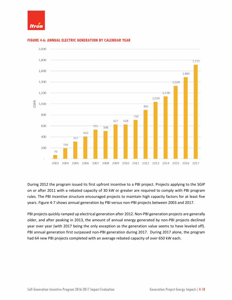
Self-Generation Incentive Program 2016-2017 Impact Evaluation Generation Project Energy Impacts|4-10
FIGURE 4-6: ANNUAL ELECTRIC GENERATION BY CALENDAR YEAR
During 2012 the program issued its first upfront incentive to a PBI project. Projects applying to the SGIP on or after 2011 with a rebated capacity of 30 kW or greater are required to comply with PBI program rules. The PBI incentive structure encouraged projects to maintain high capacity factors for at least five years. Figure 4-7 shows annual generation by PBI versus non-PBI projects between 2003 and 2017.
PBI projects quickly ramped up electrical generation after 2012. Non-PBI generation projects are generally older, and after peaking in 2013, the amount of annual energy generated by non-PBI projects declined year over year (with 2017 being the only exception as the generation value seems to have leveled off). PBI annual generation first surpassed non-PBI generation during 2017. During 2017 alone, the program had 64 new PBI projects completed with an average rebated capacity of over 650 kW each.

Self-Generation Incentive Program 2016-2017 Impact Evaluation Generation Project Energy Impacts|4-11
FIGURE 4-7: ANNUAL ELECTRIC GENERATION BY PBI VS. NON-PBI
Since its inception the SGIP has offered incentives for both renewable and non-renewable generation technologies. Beginning in 2017, the SGIP was modified such that all non-renewable projects must consume at least 10% biogas. These percentages increase each year leading ultimately to the phaseout of non-renewable generation as an eligible technology in the SGIP. No non-renewable projects subject to these new biogas blending requirements were completed and issued incentives on or before December 31, 2017. Consequently, this report does not yet quantify the impact of the new biogas blending rules. Figure 4-8 shows annual generation between 2003 and 2017 by two groups: non-renewable fueled projects and the combination of all other fuel types (including other technologies with no fuel).

Self-Generation Incentive Program 2016-2017 Impact Evaluation Generation Project Energy Impacts|4-12
FIGURE 4-8: ANNUAL ELECTRIC GENERATION BY FUEL SOURCE
Non-renewable annual generation has exceeded generation by the combination of all other fuel types every year. Non-renewable generation surpassed 1 TWh for the first time during 2016. Annual generation from the combination of all other fuel types has been rather consistent every year, although 2017 saw an increase of 11%.
Figure 4-9 shows the composition of annual electric generation by technology type from 2003 to 2017. Internal combustion engines have always contributed a large share of the annual generation. Microturbines have contributed a small but steady share of annual electric generation since 2006. Gas turbines have also contributed a steady share since 2009. Growth in annual generation since 2011 has been driven primarily by electric-only fuel cells. Electric-only fuel cells have become and are likely to remain the predominant contributor to annual generation for several more years. CHP fuel cell annual generation peaked during 2013 and has dropped slightly since then. Wind turbines contribute to a small portion of the annual generation. Since 2013 electric-only fuel cells have continued to make the largest contributions to annual generation, followed by IC engines and gas turbines.

Self-Generation Incentive Program 2016-2017 Impact Evaluation Generation Project Energy Impacts|4-13
FIGURE 4-9: ANNUAL ELECTRIC GENERATION BY TECHNOLOGY
4.1.2 Coincident Peak Demand Impacts
Coincident peak demand impacts are defined as the generation from SGIP projects during hours of CAISO or IOU peak demands. The single greatest annual CAISO or IOU peak hours provide brief snapshots of program coincident demand impacts. We consider generation during those hours as well as a more robust picture based upon average generation coincident with the annual top 200 CAISO and IOU peak hours.
By coincidentally generating during CAISO or IOU peak hours, SGIP project hosts allow their electric utility to avoid the purchase of high cost wholesale energy. At the same time the electric utility reduces its transmission and distribution losses during what typically are hours of high system congestion. Ideally, SGIP system hosts are generating at full capacity and avoiding system maintenance during peak hours and thus contributing the greatest possible demand impacts. However, these hours are not necessarily when an SGIP system host has its highest load or otherwise might want to be generating.
In this section, we examine generation during CAISO and IOU annual peak load hours as well as their top 200 load hours. We also look at year to year trends in program impacts. Table 4-10 lists hours and magnitudes of CAISO and IOU peak demands in 2016 and 2017.

Self-Generation Incentive Program 2016-2017 Impact Evaluation Generation Project Energy Impacts|4-14
TABLE 4-10: 2016 AND 2017 CAISO AND IOU PEAK HOURS AND DEMANDS [MW]
IOU
2016 2017
Peak Demand [MW] Date
Hour Beginning
[Local Time]
Peak Demand [MW] Date
Hour Beginning
[Local Time]
CAISO 45,981 Wednesday, July 27th 3:00 PM 49,909 Thursday,
September 1st 3:00 PM
PG&E 20,408 Wednesday, July 27th 4:00 PM 21,713 Thursday,
September 1st 4:00 PM
SCE 23,564 Monday, June 20th 2:00 PM 24,177 Thursday,
September 1st 2:00 PM
SDG&E 4,262 Friday, July 22nd 4:00 PM 4,481 Thursday, September 1st 3:00 PM
CAISO Peak Hour
Generation coincident with the CAISO annual peak hours in 2016 and 2017 is shown by PA in Table 4-11. The generation from SGIP projects of 175.5 MW coincident with the 2016 CAISO peak hour is equivalent to 0.38% of the 2016 CAISO peak load. During 2017, SGIP projects generated 199.2 MW during the CAISO peak hour, equivalent to 0.40% of the 2017 CAISO peak load. CAISO peak hour generation increased by 13.5% in 2017.
PG&E projects contributed the largest portions of the CAISO peak hour generation in both 2016 and 2017. SCG followed with almost a third of the total 2017 peak generation.
TABLE 4-11: 2016 AND 2017 CAISO PEAK HOUR GENERATION BY PA
Program Administrator
2016 2017
Peak Hour Generation [MW] Percent of Total Peak Hour
Generation [MW] Percent of Total
CSE 24.0 14% 20.4 10% PG&E 76.5 44% 86.8 44% SCE 31.8 18% 36.2 18% SCG 43.3 25% 55.8 28%
Total 175.5 100% 199.2 100%
Figure 4-10 and Table 4-12 on the following page show peak hour generation by PA for PBI versus non-PBI projects. Many of the trends observed during CAISO peak hours are similar to those observed for annual generation impacts.

Self-Generation Incentive Program 2016-2017 Impact Evaluation Generation Project Energy Impacts|4-15
FIGURE 4-10: NON-PBI VS PBI CAISO PEAK HOUR GENERATION BY PA AND YEAR [MW]
Table 4-12 shows non-PBI projects generated 96.9 MW during the 2016 CAISO peak. By the 2017 CAISO peak, coincident generation from these projects dropped almost 12% to only 85.4 MW. CSE and PG&E had declining contributions from non-PBI projects, while SCE and SCG saw a minor increase.
TABLE 4-12: 2016 AND 2017 CAISO PEAK HOUR GENERATION BY PA AND PBI VS NON-PBI [MW]
Program Administrator
2016 2017 Non-PBI PBI PBI Percent Non-PBI PBI PBI Percent
CSE 13.4 10.5 44% 8.9 11.5 56% PG&E 40.4 36.1 47% 33.1 53.7 62% SCE 13.5 18.2 57% 13.6 22.5 62% SCG 29.6 13.7 32% 29.8 26.0 47% Total 96.9 78.6 45% 85.4 113.7 57%
PBI projects made up 45% of the total 2016 CAISO peak hour coincident generation and 57% of the total 2017 CAISO peak hour coincident generation, increasing by 44% from 78.6 MW in 2016 to 113.7 MW in 2017. All PAs had increasing contributions from PBI projects.

Self-Generation Incentive Program 2016-2017 Impact Evaluation Generation Project Energy Impacts|4-16
Figure 4-11 shows 2016 and 2017 CAISO peak hour generation by technology for 2016 and 2017. During 2016 and 2017, electric-only fuel cells led CAISO peak hour generation by a significant amount. They led IC engines in 2016 by almost 23 MW and in 2017 by 47 MW.
FIGURE 4-11: 2016 AND 2017 CAISO PEAK HOUR GENERATION BY TECHNOLOGY [MW]
Table 4-13 and Table 4-14 list the CAISO peak hour generation by PA and technology for 2016 and 2017, respectively.
TABLE 4-13: 2016 CAISO PEAK HOUR GENERATION BY PA AND TECHNOLOGY [MW]
Program Admin. FC-CHP FC-Elec. GT ICE MT PRT WD Total
CSE 4.3 5.3 12.2 0.6 0.1 0.5 0.9 24.0 PG&E 2.5 36.0 3.5 25.8 4.8 0.0 4.0 76.5 SCE 2.4 16.8 0.0 7.6 1.9 0.2 2.8 31.8 SCG 2.4 11.5 14.4 12.7 2.3 0.0 0.0 43.3
Total 11.6 69.6 30.1 46.7 9.1 0.8 7.6 175.5

Self-Generation Incentive Program 2016-2017 Impact Evaluation Generation Project Energy Impacts|4-17
TABLE 4-14: 2017 CAISO PEAK HOUR GENERATION BY PA AND TECHNOLOGY [MW]
Program Admin. FC-CHP FC-Elec. GT ICE MT PRT WD Total
CSE 4.2 8.6 6.7 0.4 0.1 0.4 0.0 20.4 PG&E 4.1 44.6 1.4 30.1 3.0 0.5 3.1 86.8 SCE 2.8 26.0 0.0 5.9 0.6 0.1 0.8 36.2 SCG 3.6 19.1 15.3 14.9 2.9 0.0 0.0 55.8
Total 14.7 98.3 23.4 51.2 6.5 1.1 3.9 199.2
Across all PAs, electric-only fuel cells generated the highest output during the 2016 and 2017 CAISO peak hours, with PG&E electric-only fuel cells leading the generation output, producing 36 MW and 44.6 MW for 2016 and 2017 respectively. PG&E IC engines followed in both years, with 25.8 MW and 30.1 MW. Overall, microturbines and CHP fuel cells made relatively small contributions to peak hour generation for all PAs. Wind and pressure reduction turbines also made minor contributions for those PAs that had any.
Figure 4-12 and Table 4-15 show CAISO peak hour generation for 2016 and 2017 by PA and fuel type.
FIGURE 4-12: 2016 AND 2017 CAISO PEAK HOUR GENERATION BY PA AND FUEL

Self-Generation Incentive Program 2016-2017 Impact Evaluation Generation Project Energy Impacts|4-18
TABLE 4-15: 2016 AND 2017 CAISO PEAK HOUR GENERATION BY PA AND FUEL SOURCE [MW]
Program Admin.
2016 2017
Renew. DBG Other Non-Renew.
% Non-Renew. Renew. DBG Other Non-
Renew. % Non-Renew.
CSE 0.9 4.2 1.4 17.4 73% 0.7 4.4 0.4 14.9 73% PG&E 9.1 6.1 4.0 57.3 75% 12.4 6.4 3.6 64.4 74% SCE 4.6 2.7 3.0 21.4 67% 4.0 5.1 1.0 26.1 72% SCG 1.5 0.5 - 41.3 95% 2.8 2.8 - 50.2 90%
Total 16.1 13.6 8.4 137.4 78% 19.9 18.7 5.0 155.5 78%
Non-renewable fueled projects continue as the main contributors to CAISO peak hour generation, making up 78% of the total impact across both program years. The remaining fuel types contributed 38 MW in 2016 and 44 MW in 2017. PG&E and SCG saw a slight decrease in the percent of non-renewable fueled projects contributing to CAISO peak demand reductions during 2017, but the overall program did not see significant change.
Over time, generation from SGIP projects coincident with the CAISO peak hour has grown. Contributions from various categories of projects have changed with addition of new projects and retirement of old projects. Figure 4-13 through Figure 4-16 show CAISO peak hour generation trends from 2003 to 2017 by key project categories. Figure 4-13 shows the CAISO peak hour generation growth. CAISO peak impact growth has been generally consistent with a steady increase of almost 10% or higher year over year for the better part of the program.
FIGURE 4-13: CAISO PEAK HOUR GENERATION TOTAL BY CALENDAR YEAR

Self-Generation Incentive Program 2016-2017 Impact Evaluation Generation Project Energy Impacts|4-19
The share of CAISO peak hour generation for PBI projects exceeded those of non-PBI projects for the first time in 2017, while the share from non-PBI projects has been decreasing since 2014 (Figure 4-14).
FIGURE 4-14: CAISO PEAK HOUR GENERATION BY PBI VERSUS NON-PBI
Growth in CAISO peak hour generation from non-renewable fueled projects has continued to rise, as seen in Figure 4-15. However, the contribution from the combination of all other fuel types has stayed rather steady over the last five years, with a slight increase seen in 2017.
FIGURE 4-15: CAISO PEAK HOUR GENERATION BY FUEL TYPE

Self-Generation Incentive Program 2016-2017 Impact Evaluation Generation Project Energy Impacts|4-20
Finally, the trend in CAISO peak hour generation by technology shown in Figure 4-16 below mimics the trend of shown in Figure 4-9 for the trend in annual electric generation. Electric-only fuel cell growth since 2010 has increased CAISO peak hour program impact totals since 2010. Internal combustion engines have seen a slight increase, but other technologies stay relatively consistent over the last five years.
FIGURE 4-16: CAISO PEAK HOUR GENERATION BY TECHNOLOGY
IOU Peak Hour
Generation coincident with IOU annual peak hours for 2016 is shown below in Table 4-16 and Figure 4-17, while results for 2017 are displayed in Table 4-17 and Figure 4-18. Generation from SGIP systems is assigned to the IOU providing the electrical service, which is not necessarily the same as the PA. SoCal Gas projects may be electrically interconnected to a municipal utility rather than an IOU.
The 2016 PG&E peak hour generation occurred on July 27th between 3 and 4 PM [local time]. During this hour, projects electrically interconnected to PG&E’s system generated 75.6 MW. SCE’s 2016 peak hour was on July 20th between 1 and 2PM, where coincident generation was 54.8 MW. Projects interconnected to SDG&E’s electrical system reached 23.7 MW of generation during the peak hour on July 22nd, 2016 between the hours of 3 and 4 PM.
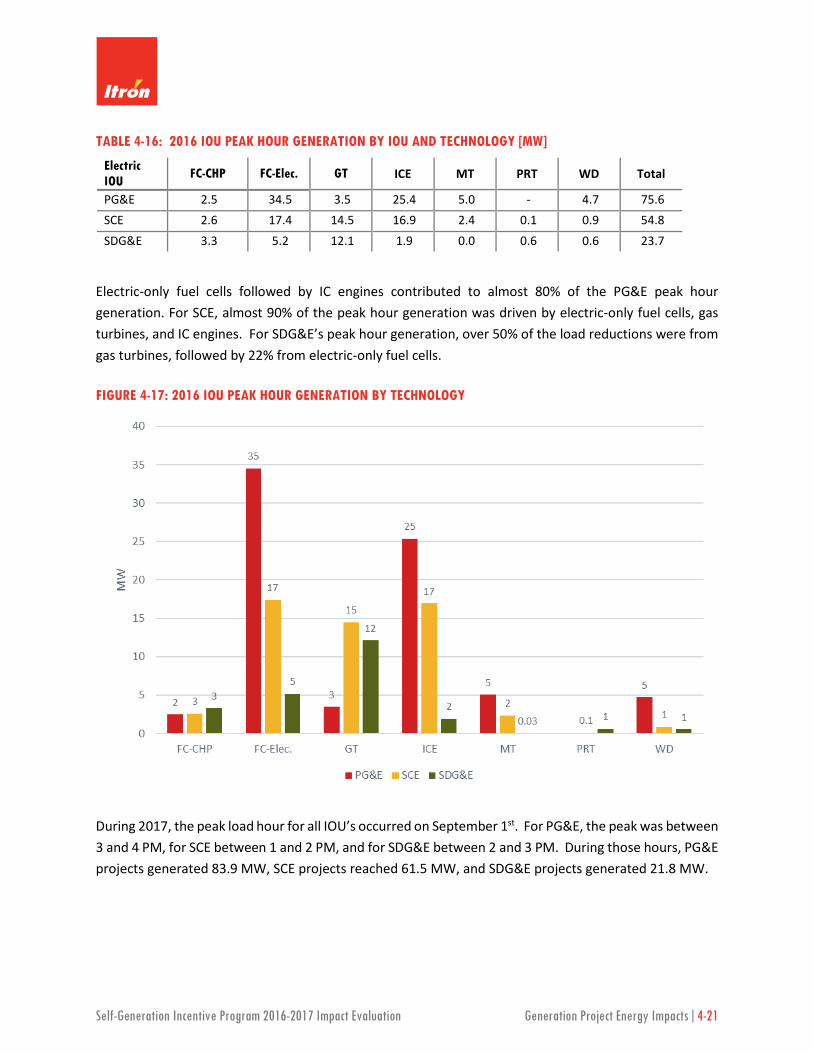
Self-Generation Incentive Program 2016-2017 Impact Evaluation Generation Project Energy Impacts|4-21
TABLE 4-16: 2016 IOU PEAK HOUR GENERATION BY IOU AND TECHNOLOGY [MW]
Electric IOU FC-CHP FC-Elec. GT ICE MT PRT WD Total
PG&E 2.5 34.5 3.5 25.4 5.0 - 4.7 75.6 SCE 2.6 17.4 14.5 16.9 2.4 0.1 0.9 54.8 SDG&E 3.3 5.2 12.1 1.9 0.0 0.6 0.6 23.7
Electric-only fuel cells followed by IC engines contributed to almost 80% of the PG&E peak hour generation. For SCE, almost 90% of the peak hour generation was driven by electric-only fuel cells, gas turbines, and IC engines. For SDG&E’s peak hour generation, over 50% of the load reductions were from gas turbines, followed by 22% from electric-only fuel cells.
FIGURE 4-17: 2016 IOU PEAK HOUR GENERATION BY TECHNOLOGY
During 2017, the peak load hour for all IOU’s occurred on September 1st. For PG&E, the peak was between 3 and 4 PM, for SCE between 1 and 2 PM, and for SDG&E between 2 and 3 PM. During those hours, PG&E projects generated 83.9 MW, SCE projects reached 61.5 MW, and SDG&E projects generated 21.8 MW.

Self-Generation Incentive Program 2016-2017 Impact Evaluation Generation Project Energy Impacts|4-22
TABLE 4-17: 2017 IOU PEAK HOUR GENERATION BY IOU AND TECHNOLOGY [MW]
Electric IOU FC-CHP FC-Elec. GT ICE MT PRT WD Total
PG&E 4.1 43.1 1.4 28.6 3.2 0.5 2.9 83.9 SCE 4.1 26.8 11.4 16.5 1.8 0.1 0.8 61.5 SDG&E 4.2 8.6 6.7 1.8 0.1 0.4 0.0 21.8
The contribution to the IOU peak hour generation for 2017 by technology didn’t change relative to 2016. Electric-only fuel cells and IC engines contributed to 85% of the PG&E peak hour generation. For SCE, almost 90% of the peak hour generation was driven by electric-only fuel cells, gas turbines, and IC engines. For SDG&E’s peak hour generation, 70% came from gas turbines and electric-only fuel cells.
FIGURE 4-18: 2017 IOU PEAK HOUR GENERATION BY TECHNOLOGY
Over time, program generation coincident with IOU peak hours has grown. Contributions by various categories of projects have changed with addition of new and retirement of old capacity. Additional information on peak hour impact trends is presented in Appendix B.

Self-Generation Incentive Program 2016-2017 Impact Evaluation Generation Project Energy Impacts|4-23
Top 200 Peak Hours
CAISO and IOU annual peak hour coincident generation is a snapshot of beneficial program impacts. Here we examine a more robust measure of impacts by examining average generation coincident with the annual top 200 CAISO and IOU peak hours. Representing just 2.3% of all hours in a year, the top 200 peak hours capture the steepest part of load distribution curves. Figure 4-19 shows the 2017 CAISO and IOU load distribution curves and indicates the 200-hour mark as the solid lime green bar on the left side.
FIGURE 4-19: 2017 CAISO AND IOU LOAD DISTRIBUTION CURVES
* Axes are scaled on left for CAISO and on right for the IOUs
The distributions of top 200 hours over the course of a year differ between CAISO and the three IOUs, as well as from year to year. While generally mid-to-late summer weekday afternoon occurrences, a top-200 hour can occur on weekends and all the way into October. Table 4-18 through Table 4-21 display the distribution of top 200 peak hours for months and weekday types of 2016 and 2017.

Self-Generation Incentive Program 2016-2017 Impact Evaluation Generation Project Energy Impacts|4-24
TABLE 4-18: 2016 TOP 200 PEAK HOUR DISTRIBUTIONS BY MONTH
TABLE 4-19: 2016 TOP 200 PEAK HOUR DISTRIBUTIONS BY WEEKDAY
TABLE 4-20: 2017 TOP 200 PEAK HOUR DISTRIBUTIONS BY MONTH
TABLE 4-21: 2017 TOP 200 PEAK HOUR DISTRIBUTIONS BY WEEKDAY
During 2016, the top 200 peak hours generally occurred June through August, with SDG&E seeing some significant hours into September. In contrast, 2017 hours seemed to be shifted by a month, with July through September typically seeing the majority of the peak hours. For CAISO and all IOUs, weekdays dominated top hours, but weekends included some top hours in both 2016 and 2017. Between 15% and 25% of peak hours occurred during the weekends, with 2017 seeing a greater percentage of hours on weekends.
May June July August September OctoberCAISO 0 46 90 55 9 0PG&E 5 57 80 39 19 0SCE 0 44 86 60 10 0SDG&E 0 20 76 64 40 0
Saturday Sunday WeekdayCAISO 27 9 164PG&E 29 9 162SCE 20 9 171SDG&E 25 4 171
May June July August September OctoberCAISO 0 25 57 75 43 0PG&E 0 52 49 55 44 0SCE 0 17 59 80 37 7SDG&E 0 7 42 76 51 24
Saturday Sunday WeekdayCAISO 30 18 152PG&E 27 24 149SCE 30 16 154SDG&E 28 14 158

Self-Generation Incentive Program 2016-2017 Impact Evaluation Generation Project Energy Impacts|4-25
Figure 4-20 shows total program generation coincident with the three IOU and CAISO 2017 peak hours, alongside average program generation coincident with the 2017 top 200 peak hours. Peak hour generation and top 200 average generation during 2017 were within a few percent of each other, except for SDG&E which saw almost a 40% increase in top 200-hour generation relative to the peak hour generation.
FIGURE 4-20: 2017 CAISO AND IOU PEAK AND TOP 200 PEAK HOUR GENERATION BY SGIP PROJECTS
CAISO peak hour and top 200 average generation impacts by technology are shown in Table 4-22 for 2016 and 2017. PG&E comparisons for 2016 and 2017 are shown in Table 4-23, SCE comparisons in Table 4-24, and SDG&E comparisons in Table 4-25.
To compare peak hour values to averages across the top 200 peak hours, the tables below show percentages of average to peak hour generation. Although many of the technologies that contribute the least to the peak hours show a large variation between peak hour and top 200 averages, technologies like electric-only fuel cells, IC engines, and gas turbine percentages are within ±10% of the top 200 hours, indicating that for the overall program, the peak hour impact is a fairly robust measure of top 200-hour impact.
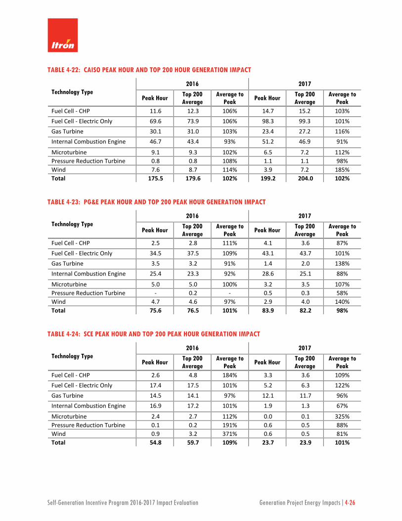
Self-Generation Incentive Program 2016-2017 Impact Evaluation Generation Project Energy Impacts|4-26
TABLE 4-22: CAISO PEAK HOUR AND TOP 200 HOUR GENERATION IMPACT
Technology Type 2016 2017
Peak Hour Top 200 Average
Average to Peak Peak Hour Top 200
Average Average to
Peak Fuel Cell - CHP 11.6 12.3 106% 14.7 15.2 103% Fuel Cell - Electric Only 69.6 73.9 106% 98.3 99.3 101% Gas Turbine 30.1 31.0 103% 23.4 27.2 116% Internal Combustion Engine 46.7 43.4 93% 51.2 46.9 91%
Microturbine 9.1 9.3 102% 6.5 7.2 112% Pressure Reduction Turbine 0.8 0.8 108% 1.1 1.1 98% Wind 7.6 8.7 114% 3.9 7.2 185% Total 175.5 179.6 102% 199.2 204.0 102%
TABLE 4-23: PG&E PEAK HOUR AND TOP 200 PEAK HOUR GENERATION IMPACT
Technology Type 2016 2017
Peak Hour Top 200 Average
Average to Peak Peak Hour Top 200
Average Average to
Peak Fuel Cell - CHP 2.5 2.8 111% 4.1 3.6 87% Fuel Cell - Electric Only 34.5 37.5 109% 43.1 43.7 101% Gas Turbine 3.5 3.2 91% 1.4 2.0 138% Internal Combustion Engine 25.4 23.3 92% 28.6 25.1 88%
Microturbine 5.0 5.0 100% 3.2 3.5 107% Pressure Reduction Turbine - 0.2 - 0.5 0.3 58% Wind 4.7 4.6 97% 2.9 4.0 140% Total 75.6 76.5 101% 83.9 82.2 98%
TABLE 4-24: SCE PEAK HOUR AND TOP 200 PEAK HOUR GENERATION IMPACT
Technology Type 2016 2017
Peak Hour Top 200 Average
Average to Peak Peak Hour Top 200
Average Average to
Peak Fuel Cell - CHP 2.6 4.8 184% 3.3 3.6 109% Fuel Cell - Electric Only 17.4 17.5 101% 5.2 6.3 122% Gas Turbine 14.5 14.1 97% 12.1 11.7 96% Internal Combustion Engine 16.9 17.2 101% 1.9 1.3 67%
Microturbine 2.4 2.7 112% 0.0 0.1 325% Pressure Reduction Turbine 0.1 0.2 191% 0.6 0.5 88% Wind 0.9 3.2 371% 0.6 0.5 81% Total 54.8 59.7 109% 23.7 23.9 101%

Self-Generation Incentive Program 2016-2017 Impact Evaluation Generation Project Energy Impacts|4-27
TABLE 4-25: SDG&E PEAK HOUR AND TOP 200 PEAK HOUR GENERATION IMPACT
Technology Type 2016 2017
Peak Hour Top 200 Average
Average to Peak Peak Hour Top 200
Average Average to
Peak Fuel Cell - CHP 4.1 3.6 87% 4.2 5.2 124% Fuel Cell - Electric Only 26.8 27.3 102% 8.6 8.6 100% Gas Turbine 11.4 12.7 112% 6.7 13.5 201% Internal Combustion Engine 16.5 16.1 97% 1.8 1.7 94%
Microturbine 1.8 2.3 127% 0.1 0.1 128% Pressure Reduction Turbine 0.1 0.3 184% 0.4 0.5 120% Wind 0.8 2.8 372% - 0.4 - Total 61.5 64.9 106% 21.8 30.0 138%
4.1.3 Noncoincident Customer Peak Demand Impacts
SGIP projects impact customer demand in addition to system (IOU or CAISO) coincident peak demand. It is not always the case that a customer’s peak demand falls on the CAISO or IOU peak load hour. The peak customer demand during any stated period is called the customer noncoincident peak (NCP) demand. The first metric this sub-section looks at is the impact on customer’s annual peak demand, which is important for understanding, the total reduction SGIP has on customer loads.
The demand portion of customer bills is based on the monthly peak kW. Thus, in addition to the reduction in annual peak demand, the monthly demand reduction illustrates how SGIP impacts customer energy costs.
Approach for Noncoincident Customer Peak Demand Impacts
To analyze the impact of SGIP on NCP customer demand, we first aligned the available load and generation data on an hourly basis. We then calculated what the gross demand would have been without the presence of the SGIP generation as the following:7
𝑮𝑮𝑮𝑮𝑮𝑮𝑮𝑮𝑮𝑮 𝑳𝑳𝑮𝑮𝑳𝑳𝑳𝑳 �𝒌𝒌𝒌𝒌������ = 𝑀𝑀𝑀𝑀𝑀𝑀𝑀𝑀𝑀𝑀𝑀𝑀𝑀𝑀 𝐿𝐿𝐿𝐿𝐿𝐿𝑀𝑀�𝒌𝒌𝒌𝒌������ + 𝐺𝐺𝑀𝑀𝐺𝐺𝑀𝑀𝑀𝑀𝐿𝐿𝑀𝑀𝐺𝐺𝐿𝐿𝐺𝐺�𝒌𝒌𝒌𝒌������ EQUATION 4-1
𝑁𝑁𝑀𝑀𝑀𝑀 𝑳𝑳𝑮𝑮𝑳𝑳𝑳𝑳 �𝒌𝒌𝒌𝒌������ = 𝑀𝑀𝑀𝑀𝑀𝑀𝑀𝑀𝑀𝑀𝑀𝑀𝑀𝑀 𝐿𝐿𝐿𝐿𝐿𝐿𝑀𝑀�𝒌𝒌𝒌𝒌������ EQUATION 4-2
7 For this analysis, demand is calculated as the average power draw within a one-hour period. This is an
approximate calculation, as demand is measured in 15-minute intervals and may differ from the hourly average.

Self-Generation Incentive Program 2016-2017 Impact Evaluation Generation Project Energy Impacts|4-28
The potential impact of SGIP generators on gross and net load can be seen graphically in the following figures. Figure 4-21 shows an example of how metered NCP customer demand, represented by net load, is reduced by SGIP generation. Figure 4-22 illustrates the impact an SGIP generator outage has on NCP customer demand. Depending on the customer load profile, a generator outage can likely set the monthly or annual peak demand.
FIGURE 4-21: EXAMPLE DEMAND IMPACTS FROM GENERATOR WITH CONSISTENT OUTPUT AND SUMMER PEAKS
FIGURE 4-22: EXAMPLE DEMAND IMPACTS FROM GENERATOR WITH OUTAGE

Self-Generation Incentive Program 2016-2017 Impact Evaluation Generation Project Energy Impacts|4-29
On a monthly basis, the impact of SGIP generation on demand is approximately:
𝑴𝑴𝑳𝑳𝑴𝑴�𝑮𝑮𝑮𝑮𝑮𝑮𝑮𝑮𝑮𝑮 𝑳𝑳𝑮𝑮𝑳𝑳𝑳𝑳 �𝒌𝒌𝒌𝒌�������𝒎𝒎𝑮𝑮𝒎𝒎𝒎𝒎𝒎𝒎
−𝑴𝑴𝑳𝑳𝑴𝑴�𝑵𝑵𝑵𝑵𝒎𝒎 𝑳𝑳𝑮𝑮𝑳𝑳𝑳𝑳 �𝒌𝒌𝒌𝒌�������𝒎𝒎𝑮𝑮𝒎𝒎𝒎𝒎𝒎𝒎
EQUATION 4-3
and on an annual basis:
𝑀𝑀𝐿𝐿𝑀𝑀�𝐺𝐺𝑀𝑀𝐿𝐿𝐺𝐺𝐺𝐺 𝐿𝐿𝐿𝐿𝐿𝐿𝑀𝑀 �𝑘𝑘𝑘𝑘�������𝑦𝑦𝑦𝑦𝑦𝑦𝑦𝑦 − 𝑀𝑀𝐿𝐿𝑀𝑀�𝑁𝑁𝑀𝑀𝑀𝑀 𝐿𝐿𝐿𝐿𝐿𝐿𝑀𝑀 �𝑘𝑘𝑘𝑘�������𝑦𝑦𝑦𝑦𝑦𝑦𝑦𝑦 EQUATION 4-4
Annual NCP Customer Demand Impacts
The average impacts of non-AES technologies on NCP customer demand are shown below in Figure 4-23 as a fraction of rebated capacity. PBI projects delivered demand savings of about 60% to 70% of their capacity; so a 1 MW project would, on average, reduce NCP customer demand by about 600-700 kW. Non-PBI projects show a much lower percentage, 38% to 40%, in part due to these being older systems.
The percent reduction of rebated capacity shown in the figures below are calculated as:
𝑃𝑃𝑀𝑀𝑀𝑀𝑃𝑃𝑀𝑀𝐺𝐺𝑀𝑀 𝑅𝑅𝑀𝑀𝑀𝑀𝑅𝑅𝑃𝑃𝑀𝑀𝐺𝐺𝐿𝐿𝐺𝐺𝑦𝑦𝑦𝑦𝑦𝑦𝑦𝑦 = �𝑀𝑀𝑀𝑀𝑀𝑀𝑀𝑀ℎ𝑙𝑙𝑦𝑦 𝑃𝑃𝑦𝑦𝑦𝑦𝑃𝑃 𝑅𝑅𝑦𝑦𝑅𝑅𝑅𝑅𝑅𝑅𝑀𝑀𝑅𝑅𝑀𝑀𝑀𝑀 (𝑃𝑃𝑘𝑘�����)𝑅𝑅𝑦𝑦𝑅𝑅𝑦𝑦𝑀𝑀𝑦𝑦𝑅𝑅 𝐶𝐶𝑦𝑦𝐶𝐶𝑦𝑦𝑅𝑅𝑅𝑅𝑀𝑀𝑦𝑦
��������������������������������� EQUATION 4-5
FIGURE 4-23: ANNUAL NCP CUSTOMER DEMAND IMPACTS

Self-Generation Incentive Program 2016-2017 Impact Evaluation Generation Project Energy Impacts|4-30
The average reduction in annual NCP across the population was 56% in 2016 and 64% in 2017. Load data were unavailable for PBI gas turbines and pressure reduction turbines, so they were not included in this analysis.
Annual NCP Customer Demand Impacts by Technology
Different technologies have significantly different impacts on annual NCP customer demand. Like Figure 4-23 above, Figure 4-24 and Figure 4-25 (on the following page) show the average demand impact as a percent of rebated capacity, but for different technologies and by PBI versus non-PBI. Figure 4-24 shows NCP demand impacts for 2016, and Figure 4-25 shows impacts for 2017.
FIGURE 4-24: ANNUAL 2016 NCP CUSTOMER DEMAND IMPACTS BY TECHNOLOGY
* This figure and the associated analysis exclude technology/incentive type pairings where the sample size was less than three.

Self-Generation Incentive Program 2016-2017 Impact Evaluation Generation Project Energy Impacts|4-31
FIGURE 4-25: ANNUAL 2017 NCP CUSTOMER DEMAND IMPACTS BY TECHNOLOGY
* This figure and the associated analysis exclude technology/incentive type pairings where the sample size was less than three.
Figure 4-24 and Figure 4-25 show that PBI projects in general exhibit larger NCP demand reductions relative to non-PBI projects. One exception is microturbines in 2017, which saw a slight decrease in percent reduction relative to their rebated capacity. The small sample size of four projects, combined with the fact that three of the four PBI microturbines in 2017 were not operating for over half of the year were important drivers for the low percentage.
Average Monthly NCP Customer Demand Reductions
Reduction to annual NCP customer demand is one metric to measure the demand savings of SGIP that aligns with some policy decisions (NEM and AB 162 (Gordon/Skinner)). Another useful metric that is relevant to host customers is average monthly demand reduction, since demand charges are billed on a monthly basis.
The percent reduction of demand shown in the figures below is calculated as:
𝑃𝑃𝑀𝑀𝑀𝑀𝑃𝑃𝑀𝑀𝐺𝐺𝑀𝑀 𝑅𝑅𝑀𝑀𝑀𝑀𝑅𝑅𝑃𝑃𝑀𝑀𝐺𝐺𝐿𝐿𝐺𝐺𝑦𝑦𝑦𝑦𝑦𝑦𝑦𝑦 = �𝑀𝑀𝑀𝑀𝑀𝑀𝑀𝑀ℎ𝑙𝑙𝑦𝑦 𝑃𝑃𝑦𝑦𝑦𝑦𝑃𝑃 𝑅𝑅𝑦𝑦𝑅𝑅𝑅𝑅𝑅𝑅𝑀𝑀𝑅𝑅𝑀𝑀𝑀𝑀 (𝑃𝑃𝑘𝑘�����)𝑀𝑀𝑀𝑀𝑀𝑀𝑀𝑀ℎ𝑙𝑙𝑦𝑦 𝐺𝐺𝑦𝑦𝑀𝑀𝐺𝐺𝐺𝐺 𝐿𝐿𝑀𝑀𝑦𝑦𝑅𝑅 (𝑃𝑃𝑘𝑘�����)
��������������������������������� EQUATION 4-6
Figure 4-26 and Figure 4-27 show similar results to the annual demand reductions. SGIP generation technologies, on average, provided monthly reductions in noncoincident customer peak demand.

Self-Generation Incentive Program 2016-2017 Impact Evaluation Generation Project Energy Impacts|4-32
FIGURE 4-26: 2016 AVERAGE MONTHLY NCP CUSTOMER DEMAND REDUCTION BY TECHNOLOGY
* This figure and the associated analysis exclude technology/incentive type pairings where the sample size was less than three.
FIGURE 4-27: 2017 AVERAGE MONTHLY NCP CUSTOMER DEMAND REDUCTION BY TECHNOLOGY
* This figure and the associated analysis exclude technology/incentive type pairings where the sample size was less than three.

Self-Generation Incentive Program 2016-2017 Impact Evaluation Generation Project Energy Impacts|4-33
4.2 UTILIZATION AND CAPACITY FACTORS
Energy impacts are a function of generating capacity and utilization. Capacity factor (CF) is a metric of system utilization. Capacity factor is defined as the amount of energy generated during a given time period divided by the maximum possible amount of energy that could have been generated during that time period. The closer the capacity factor is to one for a period indicates a system that is being utilized to its maximum potential.
Host customers utilize their systems at capacity factors according to their individual needs. Some only need full capacity during weekday afternoons; others need full capacity 24/7. Annual capacity factors are useful when comparing utilization between or across varieties of project sizes and technologies. To the extent that SGIP projects are cleaner (with respect to greenhouse gases and criteria air pollutants) than the grid energy they displace, high annual capacity factors are desirable. A capacity factor of 1.0 is full utilization regardless of a project’s generating capacity.
The annual capacity factor of a project, CFa, is defined in Equation 4-7 as the sum of hourly electric net generation output, ENGOh, during all 8,760 hours of the year divided by the product of the project’s capacity and 8,760. If a project was completed mid-year, then the annual capacity factor is evaluated from the completion date through the end of year.
𝐶𝐶𝐹𝐹𝑦𝑦 = ∑ 𝐸𝐸𝐸𝐸𝐺𝐺𝑂𝑂ℎ[𝑃𝑃𝑘𝑘ℎ]87601
𝐶𝐶𝑦𝑦𝐶𝐶𝑦𝑦𝑅𝑅𝐶𝐶𝑀𝑀𝑦𝑦 [𝑃𝑃𝑘𝑘]×8760 [ℎ𝑦𝑦] EQUATION 4-7
When aggregating the results up to the program or technology level, projects which have been decommissioned, or showed less than 30-days of data were removed from the analysis. This allows the capacity factors to be calculated based only on projects which are known to be fully operating.
Figure 4-28 shows the annual capacity factors for the program’s seven rebated generation technologies during 2016 and 2017. Electric-only fuel cells and gas turbines showed the highest capacity factors across 2016 and 2017, followed by CHP fuel cells. IC engines, microturbines, and pressure reduction turbines all showed capacity factors in the 30% to 40% range for 2016 and 2017, except 2016 microturbines at 44%.

Self-Generation Incentive Program 2016-2017 Impact Evaluation Generation Project Energy Impacts|4-34
FIGURE 4-28: 2016 AND 2017 ANNUAL CAPACITY FACTORS BY TECHNOLOGY
Figure 4-29 shows the annual 2017 capacity factors for the seven program generation technologies, split by PBI and non-PBI projects. Across all technologies, PBI projects showed higher capacity factors, except for microturbines where the capacity factors were the same for both incentive types. The two fuel cell technologies and IC engines showed substantial differences between PBI and non-PBI capacity factors. There were no non-PBI pressure reduction turbines.
FIGURE 4-29: 2017 ANNUAL CAPACITY FACTORS BY TECHNOLOGY FOR PBI VERSUS NON-PBI
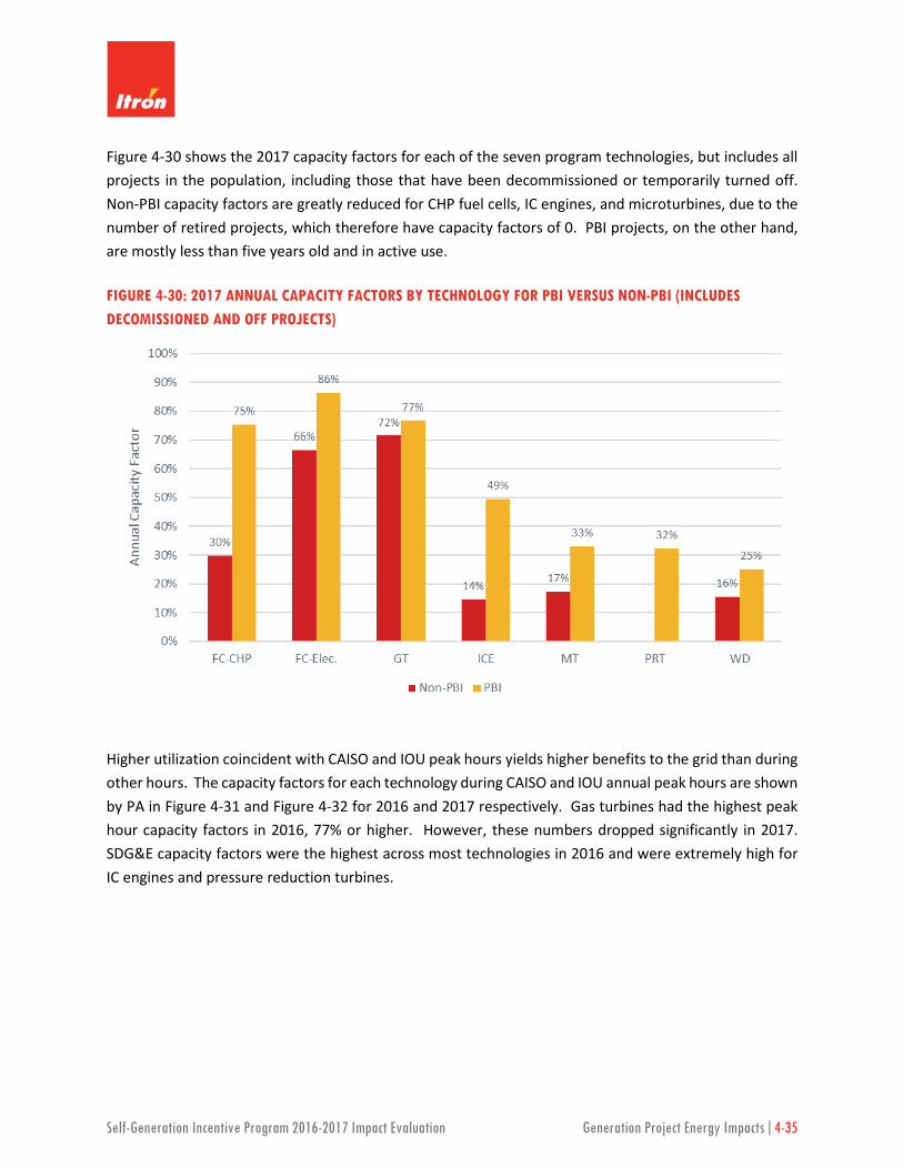
Self-Generation Incentive Program 2016-2017 Impact Evaluation Generation Project Energy Impacts|4-35
Figure 4-30 shows the 2017 capacity factors for each of the seven program technologies, but includes all projects in the population, including those that have been decommissioned or temporarily turned off. Non-PBI capacity factors are greatly reduced for CHP fuel cells, IC engines, and microturbines, due to the number of retired projects, which therefore have capacity factors of 0. PBI projects, on the other hand, are mostly less than five years old and in active use.
FIGURE 4-30: 2017 ANNUAL CAPACITY FACTORS BY TECHNOLOGY FOR PBI VERSUS NON-PBI (INCLUDES DECOMISSIONED AND OFF PROJECTS)
Higher utilization coincident with CAISO and IOU peak hours yields higher benefits to the grid than during other hours. The capacity factors for each technology during CAISO and IOU annual peak hours are shown by PA in Figure 4-31 and Figure 4-32 for 2016 and 2017 respectively. Gas turbines had the highest peak hour capacity factors in 2016, 77% or higher. However, these numbers dropped significantly in 2017. SDG&E capacity factors were the highest across most technologies in 2016 and were extremely high for IC engines and pressure reduction turbines.
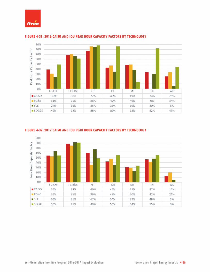
Self-Generation Incentive Program 2016-2017 Impact Evaluation Generation Project Energy Impacts|4-36
FIGURE 4-31: 2016 CAISO AND IOU PEAK HOUR CAPACITY FACTORS BY TECHNOLOGY
FIGURE 4-32: 2017 CAISO AND IOU PEAK HOUR CAPACITY FACTORS BY TECHNOLOGY

Self-Generation Incentive Program 2016-2017 Impact Evaluation Generation Project Energy Impacts|4-37
4.3 USEFUL HEAT RECOVERY
Fuel energy that enters SGIP systems is converted into electricity and heat. Certain SGIP technologies are capable of capturing this heat to usefully serve on-site end uses instead of dissipating it to the atmosphere. Except for electric-only fuel cells that achieve high fuel-to-electric conversion efficiencies, the SGIP requires useful heat recovery where natural gas is a system’s predominant fuel. Where the predominant fuel is renewable biogas an SGIP system is exempt from the heat recovery requirement. The biogas exemption from heat recovery was introduced in the program’s first year.
The end uses served by heat recovery, heating and/or cooling, have important implications for net greenhouse gas emissions. The comparable baseline measures for heating and cooling are a natural gas boiler and a grid-served electric chiller respectively. Useful heat recovery that displaces a baseline boiler will reduce emissions more than if it displaces a baseline electric chiller. The distribution of end uses served by useful heat recovery from SGIP systems is summarized in Table 4-26.
TABLE 4-26: 2017 END USES SERVED BY USEFUL RECOVERED HEAT
Useful Heat End Use Project Count Rebated Capacity [MW]
Percent of Rebated Capacity
Cooling Only 47 46.5 15% Heating Only 410 176.5 58% Heating and Cooling 95 80.1 26% Total 552 303.0 100%
* Technologies excluded from total capacity are Advanced Energy Storage, Pressure Reduction Turbines, Wind, and other generation technologies exempt from CHP requirements.
4.4 SYSTEM EFFICIENCIES
The ability to convert fuel into useful electrical and thermal energy is measured by the system’s combined efficiency in doing both. The combined or overall system efficiency is defined in Equation 4-8 as the ratio of the sum of electrical generation and useful recovered heat8 to the fuel energy input.
𝜂𝜂𝐺𝐺𝑦𝑦𝐺𝐺𝑀𝑀𝑦𝑦𝑠𝑠 = 𝐸𝐸𝐸𝐸𝐺𝐺𝑂𝑂𝑘𝑘𝑘𝑘ℎ×3.412+𝐻𝐻𝐸𝐸𝐻𝐻𝑇𝑇𝑀𝑀𝑀𝑀𝑀𝑀𝑀𝑀𝐹𝐹𝐹𝐹𝐸𝐸𝐿𝐿𝑀𝑀𝑀𝑀𝑀𝑀𝑀𝑀,𝐿𝐿𝐿𝐿𝐿𝐿
EQUATION 4-8
8 In the context of this report, useful heat is defined as heat that is recovered from CHP projects and used to
serve on-site thermal loads. Waste heat that is lost to the atmosphere or dumped via radiators is not considered useful heat.

Self-Generation Incentive Program 2016-2017 Impact Evaluation Generation Project Energy Impacts|4-38
The higher the system’s overall efficiency the less fuel input is required to produce the sum of electricity and useful recovered heat. Electric-only fuel cells do not require useful heat recovery capabilities; therefore, their system overall efficiency has only an electrical component. Technologies that recover useful heat have electrical and thermal component efficiencies. All efficiencies are reported on a lower heating value (LHV) basis.9
System overall and component efficiencies observed for non-renewable projects in 2016 and 2017 are shown in Figure 4-33 and Figure 4-34, with electrical conversion efficiency shown in yellow, thermal efficiency shown in red, and overall system efficiency representing the sum of both components. Both figures below also display green bars over each technology, which represent the program minimum overall efficiency targets of 54.1% LHV (or 60% HHV) for CHP and 36.1% LHV (40% HHV) for electric-only fuel cells.
During 2016 and 2017, IC engines and microturbines lagged behind their efficiency targets by approximately 20%, while fuel cell technologies and gas turbines exceeded their targets. Deficiencies in a system efficiency are almost always related to useful heat recovery and utilization. The electrical efficiency of CHP prime movers is not typically variable – there are some variances in efficiency as a function of air inlet temperature and therefore seasons, but these are minor.
FIGURE 4-33: 2016 OVERALL AND COMPONENT LHV EFFICIENCIES BY TECHNOLOGY
9 This evaluation report assumes a natural gas lower heating value energy content of 934.9 Btu/SCF and higher
heating content of 1036.6 Btu/SCF for an LHV/HHV ratio of 0.9019 (Combined Heating, Cooling & Power Handbook: Technologies & Applications. Neil Petchers. The Fairmont Press, 2003.)

Self-Generation Incentive Program 2016-2017 Impact Evaluation Generation Project Energy Impacts|4-39
FIGURE 4-34: 2017 OVERALL AND COMPONENT LHV EFFICIENCIES BY TECHNOLOGY
A system’s ability to meet efficiency requirements is almost always tied to its heat recovery system. This is also the most complicated engineering challenge when implementing CHP. If the CHP generator is not appropriately sized to the annual heating and cooling loads of a building, then much of the excess heat must be dumped to the atmosphere through a radiator. Useful heat recovery loops may also be temporarily shut down due to maintenance issues. These types of events can cause a technology to have a low useful heat recovery rate and therefore a low system efficiency.
Projects subject to PBI payment rules are expected to perform better than older non-PBI projects which receive their payments up front. This is seen below in Figure 4-35 and Figure 4-36 for 2016 and 2017 respectively. The reason PBI projects typically perform better than their non-PBI counterparts can be explained by the fact that these are typically newer projects, and they are incentivized to keep the projects running as efficiently as possible. CHP fuel cells are the only technology where the non-PBI systems appeared to be performing better than the PBI projects. However, this is likely driven by the small sample of projects where enough metering data were available to calculate efficiencies.

Self-Generation Incentive Program 2016-2017 Impact Evaluation Generation Project Energy Impacts|4-40
FIGURE 4-35: 2016 OVERALL AND COMPONENT LHV EFFICIENCIES BY TECHNOLOGY FOR PBI VERUSUS NON-PBI
FIGURE 4-36: 2017 OVERALL AND COMPONENT LHV EFFICIENCIES BY TECHNOLOGY FOR PBI VERUSUS NON-PBI

Self-Generation Incentive Program 2016-2017 Impact Evaluation Generation Project Energy Impacts|4-41
4.5 NATURAL GAS IMPACTS
The use of natural gas fuel by many SGIP systems results in increased pipeline transport of natural gas in California. The useful recovery of heat that displaces natural gas boilers mitigates this increase to some extent. Figure 4-37 shows the gross and net natural gas consumption from 2003 to 2017 in millions of Therms. The total column height is the gross consumption by SGIP systems. The red upper portion of the column is consumption avoided by recovering waste heat to displace boilers. The yellow lower portion of the column then is the net consumption. The values shown on the lower portions are net consumption.
FIGURE 4-37: ANNUAL NATURAL GAS CONSUMPTION BY SGIP PROJECTS
Figure 4-38 shows natural gas impacts during 2016 and 2017 by technology. All-electric fuel cells showed the highest natural gas impact, almost double that of gas turbines and IC engines, which makes sense as the electrical energy generated by all-electric fuel cells made up almost 50% of the all non-AES impacts during 2017. On a per-electrical energy generation basis, microturbines had the higher natural gas impact at a rate of 0.13 million therms per GWh, followed by gas turbines at 0.09 and then IC engines at 0.07. Both electric-only and CHP fuel cells generated the lowest natural gas impact at 0.06 million therms per GWh.
Figure 4-39 displays the growth in natural gas consumption from 2003 to 2017 by technology.

Self-Generation Incentive Program 2016-2017 Impact Evaluation Generation Project Energy Impacts|4-42
FIGURE 4-38: 2016 AND 2017 NATURAL GAS NET IMPACTS BY TECHNOLOGY
FIGURE 4-39: ANNUAL NATURAL GAS IMPACTS BY TECHNOLOGY

Self-Generation Incentive Program 2016-2017 Impact Evaluation Generation Project Energy Impacts|4-43
4.6 MARGINAL COST IMPACTS
Utility marginal cost impacts were calculated for each technology type. The marginal costs used in our analysis are based on the Energy and Environmental Economics (E3) Distributed Energy Resource (DER) Avoided Cost Calculator. 10 Utility marginal costs impacts are a function of the annual energy generated. The components of the total utility marginal costs include ancillary services, distribution costs, energy costs, RPS costs, and capacity costs.
The different components of the total utility marginal costs are shown below in Figure 4-40 by IOU and year, on an avoided cost per rebated kW basis. SDG&E saw the highest avoided costs per rebated kW, achieving almost $400 per rebated kW in 2017. PG&E saw avoided costs of $336 per rebated kW, and SCE saw $284 per rebated kW in 2017.
FIGURE 4-40: MARGINAL AVOIDED COSTS $ PER REBATED CAPACITY [KW] BY IOU AND YEAR
10 Documentation for the 2018 DER Avoided Cost Calculator and Documentation, used for the 2017 analysis are
available at: http://www.cpuc.ca.gov/General.aspx?id=5267

Self-Generation Incentive Program 2016-2017 Impact Evaluation Generation Project Energy Impacts|4-44
Figure 4-41 shows the total utility marginal avoided costs, in millions of dollars, by IOU and year. As 2017 saw higher energy generated than 2016, the utility avoided costs across all IOUs were higher in 2017 than 2016. PG&E saw the overall highest total marginal avoided costs, avoiding over $63 million in 2017 and over $42 million in 2016.
FIGURE 4-41: TOTAL MARGINAL AVOIDED COSTS [MILLIONS $] BY IOU AND YEAR

Self-Generation Incentive Program 2016-2017 Impact Evaluation Advanced Energy Storage Impacts|5-1
5 ADVANCED ENERGY STORAGE IMPACTS This section describes the performance metrics, customer impacts, CAISO and IOU system impacts, utility marginal cost impacts, and population impacts for the AES program populations at the end of 2016 and 2017. These analyses are drawn from the 2016 and 2017 SGIP Advanced Energy Storage Impact Evaluations.1
5.1 PERFORMANCE METRICS
5.1.1 Capacity Factor and Roundtrip Efficiency
Capacity factor is a measure of system utilization. It is defined as the sum of the storage discharge (in kWh) divided by the maximum possible discharge within a given time period. This is based on the SGIP rebated capacity of the system (in kW) and the total hours of operation. The SGIP handbook assumes 5,200 maximum hours of operation in a year rather than the full 8,760 hours (60 percent). This is to account for the fact that “Advanced Energy Storage Projects typically discharge during peak weekday periods and are unable to discharge during their charging period.”2 For purposes of SGIP evaluation, the AES capacity factor is calculated as:
𝐶𝐶𝐶𝐶𝐶𝐶𝐶𝐶𝐶𝐶𝐶𝐶𝐶𝐶𝐶𝐶 𝐹𝐹𝐶𝐶𝐶𝐶𝐶𝐶𝐹𝐹𝐹𝐹 = ∑𝑘𝑘𝑘𝑘ℎ 𝐷𝐷𝐶𝐶𝐷𝐷𝐶𝐶ℎ𝐶𝐶𝐹𝐹𝑎𝑎𝑎𝑎 (𝑘𝑘𝑘𝑘ℎ)
𝐻𝐻𝐹𝐹𝐻𝐻𝐹𝐹𝐷𝐷 𝐹𝐹𝑜𝑜 𝐷𝐷𝐶𝐶𝐶𝐶𝐶𝐶 𝐴𝐴𝐴𝐴𝐶𝐶𝐶𝐶𝐴𝐴𝐶𝐶𝐴𝐴𝐴𝐴𝑎𝑎 × 𝑅𝑅𝑎𝑎𝐴𝐴𝐶𝐶𝐶𝐶𝑎𝑎𝑅𝑅 𝐶𝐶𝐶𝐶𝐶𝐶𝐶𝐶𝐶𝐶𝐶𝐶𝐶𝐶𝐶𝐶 (𝑘𝑘𝑘𝑘) × 60%
The SGIP Handbook requires that PBI projects achieve an AES capacity factor of at least 10% per the above formula, 520 hours of equivalent full discharge over the course of each year, to receive full payment.3 Non-PBI projects are not required to meet a 10% capacity factor.
Another key performance metric is roundtrip efficiency (RTE), which is an eligibility requirement for the SGIP.4 The RTE is defined as the total kWh discharge of the system divided by the total kWh charge and,
1 The 2016 and 2017 SGIP Advanced Energy Storage Impact Evaluation Reports can be found at
http://www.cpuc.ca.gov/General.aspx?id=7890 2 See 2015 SGIP Handbook, p. 37. 3 “520 discharge hours” refers to the amount energy released when discharging a battery at full capacity for 520
hours. AES projects typically discharge during peak weekday periods and are unable to discharge during their charging period. For this reason, 5,200 hours per year will be used for the purposes of calculating the capacity factor for AES projects. That is, a system may discharge at full capacity for 520 hours, or, say, 50% capacity for 1,040 hours – the amount of energy in the two is the same, each constituting 520 discharge hours.
4 AES systems must maintain a round trip efficiency equal to or greater than 69.6% in the first year of operation in order to achieve a ten-year average round trip efficiency of 66.5%, assuming a 1% annual degradation rate. (2016 SGIP Handbook, https://www.selfgenca.com/documents/handbook/2016)

Self-Generation Incentive Program 2016-2017 Impact Evaluation Advanced Energy Storage Impacts|5-2
for a given period of time, should range from 0% to 100%. For SGIP evaluation purposes, this metric was calculated for each project over the whole period for which dispatch data were available and deemed verifiable. RTEs should never be greater than 100% when calculated over the course of a couple of days or a month. The evaluation team carefully examined the RTEs for each project as part of the QC process to verify that there were no underlying data quality issues.
Project CFs and RTEs
The capacity factors for the sample of AES projects evaluated in 2016 and 2017 are presented below in Figure 5-1. The average CF for PBI projects are similar across both evaluation periods. Non-PBI projects, however, exhibited an increased utilization from 2016 to 2017. It’s important to note, the sample of non-PBI projects were different across the two program years. The different make-up of projects precludes a direct comparison across the years. We do, however, provide a high-level comparison of CFs for projects that were evaluated in both years. These comparisons are presented in the following section. Residential projects were not evaluated in 2016. The sample of projects in 2017 exhibited an SGIP capacity factor of 0.02.
FIGURE 5-1: HISTOGRAM OF AES DISCHARGE CAPACITY FACTOR BY CALENDAR YEAR
Figure 5-2 presents the distribution of RTEs for all sampled projects in 2016 and 2017. PBI projects – in both years – exhibit a much higher RTE than non-PBI projects. RTEs have increased for both project types from 2016 to 2017, but again, direct comparisons should be made with caution as the sample of projects for each program year were different. Residential projects have the lowest RTE at roughly 38%.

Self-Generation Incentive Program 2016-2017 Impact Evaluation Advanced Energy Storage Impacts|5-3
FIGURE 5-2: HISTOGRAM OF NONRESIDENTIAL ROUNDTRIP EFFICIENCY BY PROGRAM YEAR
Note that by calculating the RTE over the course of several months, the metric not only captures the losses due to AC-DC power conversion but also the parasitic loads associated with system cooling, communications and other power electronic loads. Parasitic loads can represent a significant fraction of total charging energy (the denominator in the RTE calculation), especially for systems that are idle for extended periods. This relationship is exhibited in Figure 5-3 for 2016 projects and Figure 5-4 for 2017 projects. Systems with the lowest capacity factors tend to have the lowest RTEs.
FIGURE 5-3: TOTAL ROUNDTRIP EFFICIENCY VERSUS CAPACITY FACTORS (ALL 2016 PROJECTS)

Self-Generation Incentive Program 2016-2017 Impact Evaluation Advanced Energy Storage Impacts|5-4
FIGURE 5-4: TOTAL ROUNDTRIP EFFICIENCY VERSUS CAPACITY FACTORS (ALL 2017 PROJECTS)
We also examined the dispatch performance of the storage systems relative to the rebated capacity of the systems. Figure 5-5 presents the 15-minute kW storage charge (-) and discharge (+) normalized by storage system rebated capacity for non-PBI and PBI systems5 for projects evaluated in 2017. The evaluation team observed no differences in the distribution of 15-minute charge/discharge kW from the 2016 program year. For both PBI and non-PBI projects, most observations (approximately 60%) are at or near zero. This suggests that over the course of 2017 (and 2016), most systems were idle or dispatching at a small percentage of capacity. Both distributions skew towards charge, indicating more charging than discharging (as they should to have RTEs less than one). For non-PBI systems, a significant percentage (23%) of observations are slightly negative. This distribution suggests that a significant portion of non-PBI observations are spent serving parasitic loads. The charge/discharge 15-minute power for PBI projects is more normally distributed.
5 It’s important to note that the x-axis was set to -1 to 1 so that the scale of observations further from zero could
be visualized. There are 15-minute charge/discharge observations for PBI and non-PBI projects that are -/+ 2 times rebated capacity.

Self-Generation Incentive Program 2016-2017 Impact Evaluation Advanced Energy Storage Impacts|5-5
FIGURE 5-5: HISTOGRAM OF NON-PBI AND PBI NORMALIZED 15-MINUTE POWER (2017)
Again, the annual RTE is calculated over the course of several months, and the metric not only captures the losses due to AC-DC power conversion, but also the parasitic loads associated with system cooling, communications and other power electronic loads. The evaluation team observed significant differences in the way storage systems are being utilized for residential customers compared to nonresidential customers (See Customer Impact Section). Residential customers in 2017 were primarily on tariffs with a tiered pricing structure, whereas nonresidential customers were on tariffs with TOU energy rates and demand charges. SGIP requirements (52 cycles per year for residential projects compared to 130 for nonresidential, CF requirements for PBI projects and RTE program eligibility requirements for nonresidential systems) also dictate differences in the storage dispatch behavior from residential to nonresidential customers. This is evident in Figure 5-6 for the sample of 2017 projects. Residential projects were not evaluated in 2016.
The average monthly RTEs are significantly greater in the latter months of the year, namely October, November and December. The evaluation team observed more consistent, daily storage cycling from residential projects in those months. Nonresidential customers, however, are utilizing their storage systems to realize bill savings (namely non-coincident peak demand reduction), so monthly RTEs don’t vary as significantly across months as those from residential systems.

Self-Generation Incentive Program 2016-2017 Impact Evaluation Advanced Energy Storage Impacts|5-6
FIGURE 5-6: AVERAGE MONTHLY ROUNDTRIP EFFICIENCY FOR RESIDENTIAL PROJECTS (2017)
Figure 5-7 on the following page presents the number of cycling events for each residential project throughout 2017. The SGIP requires residential storage systems to cycle 52 times throughout the year.6 Twenty-one of the twenty-eight projects met the 52-cycle requirement. One project was online throughout the entirety of 2017, discharging each day throughout the afternoon hours and charging thereafter. Of the seven that did not meet the requirement, three were idle throughout the entire metering period.
6 https://www.selfgenca.com/documents/handbook/2017

Self-Generation Incentive Program 2016-2017 Impact Evaluation Advanced Energy Storage Impacts|5-7
FIGURE 5-7: ANNUAL SINGLE CYCLE EVENTS FOR SAMPLE OF RESIDENTIAL PROJECTS (2017)
Figure 5-8 presents the average number of cycles across the metered sample of 28 projects by month. This figure mirrors the RTEs presented in Figure 5-6 as more utilized systems tend to have higher RTEs and parasitic losses from idle systems generally lead to lower RTEs. In 2017, there were five to eight projects cycling throughout the early winter and summer months. Most projects begin cycling in October throughout the remainder of the year. Presumably they are programmed to meet the 52-cycle per year requirement.
FIGURE 5-8: AVERAGE MONTHLY SINGLE CYCLE EVENTS FOR SAMPLED RESIDENTIAL PROJECTS (2017)

Self-Generation Incentive Program 2016-2017 Impact Evaluation Advanced Energy Storage Impacts|5-8
5.1.2 Cross-Year Performance Impact Comparisons (2016-2017)
The evaluation team also compared the performance metrics developed from the 2016 impact evaluation to those garnered from the 2017 evaluation. These comparisons were made for project-specific RTEs and capacity factors to highlight any potential changes in operation or utilization from one year to the next. It is important to note, many projects evaluated in 2016 received their upfront payment at different times throughout the year, so the performance metrics did not incorporate a full calendar year of impacts. All projects paid incentives during 2016 were online and operating throughout the entirety of 2017, so any potential changes in performance from one year to the next may only reflect that difference.
Figure 5-9 and Figure 5-10 on the following page present those comparisons for RTEs and CFs, respectively. Any point on the figure above the black line represents a project with a greater RTE in 2017 relative to 2016. On average, non-PBI projects exhibit greater RTEs in 2017 compared to their own operation in 2016. For PBI projects, the differences are negligible. Similarly, non-PBI projects generally are being utilized more in 2017 compared to the previous year. PBI projects, however, appear to be utilized less – exhibiting lower CFs in 2017, on average, than 2016.
Again, these metrics were developed from the period of available data for each project and each calendar year. A project may have received an upfront payment in November of 2016 and the project CF would be calculated over that 2-month period. The CF for that same project, would be calculated for the entirety of 2017, where data was available and verifiable. Differences in performance across the 2 years could signal a change in operation or could represent differences in the time frame in which impacts were calculated for each year.
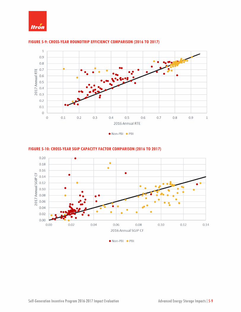
Self-Generation Incentive Program 2016-2017 Impact Evaluation Advanced Energy Storage Impacts|5-9
FIGURE 5-9: CROSS-YEAR ROUNDTRIP EFFICIENCY COMPARISON (2016 TO 2017)
FIGURE 5-10: CROSS-YEAR SGIP CAPACITY FACTOR COMPARISON (2016 TO 2017)

Self-Generation Incentive Program 2016-2017 Impact Evaluation Advanced Energy Storage Impacts|5-10
5.1.3 Influence of Parasitic Loads on Performance
The mean observed RTE for non-PBI projects (52%) was far lower than for PBI projects (81%) in 2017. Likewise, Figure 5-1 provided evidence that non-PBI systems were under-utilized with capacity factors generally ranging from 0.02 to 0.04. One consequence of this underutilization is the accumulation of standby losses and parasitic loads associated with system cooling, communications and other power electronic loads. For the 2017 evaluation, we attempted to quantify the influence of these losses by classifying the storage dispatch into three general categories:
Discharge – any 15-minute discharge (+) event
Charge – any 15-minute charge (-) event not identified as an idle/other period
Idle/Other – any 15-minute charge (-) event not identified as a charge period
─ Identify 15-minute charge (-) event when storage system is NOT discharging
─ Develop a frequency distribution of those 15-minute charge (-) events by project-specific storage system throughout the course of the year
─ Identify project-specific cut point where frequency distribution of charge kWh is obvious within the data7
─ Develop a weighted8 average of all 15-minute charge observations below the cut point
─ Set any 15-minute charge (-) event to zero if equal to or below the weighted average
Figure 5-11 presents a graphical representation of charge, discharge and idle/other designation. The 15-minute charge and discharge events are evident in the data. However, periods of inactivity (highlighted in gray) represent a small charge throughout the metering period. While the charge level is small at the 15-minute level, over the course of year, the impacts can become substantial, especially for a system that is under-utilized.
7 For example, if 60% of charge events were 0.1 kWh (400 watts), 30% were 0.2 kWh (800 watts) and the next
bin, 0.3 kWh (1,200 watts), represented 2% of all charge events, the cut point would be 0.2 kWh and below. 8 The “weight” represents the total number of observations within each 15-minute charge kWh bin. In the above
example, the weighted average would be ~ 0.133.

Self-Generation Incentive Program 2016-2017 Impact Evaluation Advanced Energy Storage Impacts|5-11
FIGURE 5-11: EXAMPLE CLASSIFICATION OF 15 MINUTE POWER KW CHARGE/DISCHARGE/IDLE
Nonresidential Parasitic Influence
Figure 5-12 and Figure 5-13 present the average mean parasitic load for each project developed using the above methodology for 2017 projects. The average parasitic load estimated at the 15-minute interval is represented on the horizontal axis and the percentage of rebated capacity each of those parasitics represent are conveyed on the vertical axis for non-PBI and PBI projects, respectively. Non-PBI projects are further split out by the building type (or facility type).
The average parasitic for non-PBI ranges from zero to roughly 0.35 kWh at the 15-minute level.9 While there is considerable variability in the range of parasitics, the magnitude of those power draws relative to system rebated capacity are all within 0% to 6% for non-PBI projects.10
9 A 15-minute kWh load of 0.35 is equivalent to 1,400 watts of power at the same time interval. 10 These systems are rated as 2 hour batteries with inverters sometimes sized 2x the rebated capacity. The
percentages on the vertical axis would be half of what is presented if the inverter size was twice the rebated capacity.
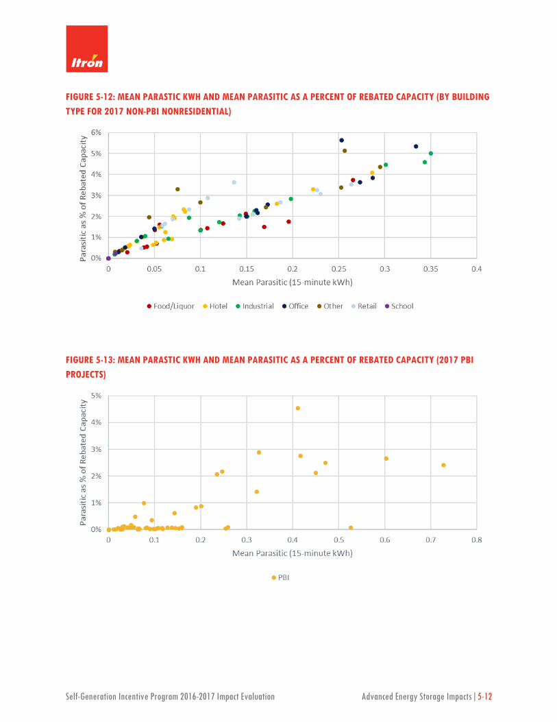
Self-Generation Incentive Program 2016-2017 Impact Evaluation Advanced Energy Storage Impacts|5-12
FIGURE 5-12: MEAN PARASTIC KWH AND MEAN PARASITIC AS A PERCENT OF REBATED CAPACITY (BY BUILDING TYPE FOR 2017 NON-PBI NONRESIDENTIAL)
FIGURE 5-13: MEAN PARASTIC KWH AND MEAN PARASITIC AS A PERCENT OF REBATED CAPACITY (2017 PBI PROJECTS)

Self-Generation Incentive Program 2016-2017 Impact Evaluation Advanced Energy Storage Impacts|5-13
We conducted an analysis on these data using the classification scheme discussed above to estimate the impact that these small parasitic loads can have on 2017 system performance. The 15-minute interval power output was set to zero for all Idle/Other observations. We then re-calculated the roundtrip efficiencies of nonresidential projects to assess the influence of those “idle” hours. The results of that analysis are presented below in Figure 5-14. The y-axis represents the system RTE with no parasitic loads and the x-axis represents the project RTE with the parasitic loads included (as observed). An observation on the black line means that the RTEs are identical – removing parasitic loads had no influence on the RTE of the system. This is mostly true for the larger PBI projects which are represented in yellow. However, for many of the non-PBI systems, removal of the parasitic loads would lead to an enhanced performance of the system. Projects in the 30% to 40% range would exhibit RTEs in the 40% to 50% range if the parasitic loads were removed.
FIGURE 5-14: INFLUENCE OF PARASITICS ON ROUNDTRIP EFFICIENCY (2017 NONRESIDENTIAL PROJECTS)
Residential Parasitic Influence
The average parasitic observed in the residential metered data was 0.09 kWh at the 15-minute interval or roughly 40 watts. As presented above in Figure 5-1, residential systems were under-utilized, especially throughout the first three quarters of 2017, so the small parasitic draw, at the 15-minute level, adds up considerably throughout the year. Projects with calculated RTEs in the 30 to 40% range would exhibit RTEs of 50 to 60% in the absence of that idle load.

Self-Generation Incentive Program 2016-2017 Impact Evaluation Advanced Energy Storage Impacts|5-14
FIGURE 5-15: INFLUENCE OF PARASITICS ON ROUNDTRIP EFFICIENCY (2017 RESIDENTIAL PROJECTS)
5.2 CUSTOMER IMPACTS
5.2.1 Nonresidential Projects
Storage systems can be utilized for a variety of use cases, and dispatch objectives are predicated on several different factors including facility load profiles, rate structures, other market-based mechanisms and reliability in the event of an outage. Customers on TOU bill rates may be incentivized to discharge energy during peak and partial-peak hours (when retail energy rates are higher) and avoid charging until off-peak hours when rates are lower. Similarly, customers that are also on a rate that assesses demand charges during peak demand periods and/or at the monthly billing level, may prioritize peak demand reduction.
TOU periods are based on sub-hourly approximations of commercial rates within each of the three California electric IOUs. During winter months and summer months – which are defined by the specific IOU rate – customers pay a different rate and, within those seasons, pay different rates for each period (peak, partial-peak and off-peak).
The evaluation team conducted several different but concurrent analyses using the above TOU period descriptions along with customer rate schedules for both the 2016 and 2017 impact evaluations. The remainder of this section presents those results in more detail. Some patterns of charge/discharge

Self-Generation Incentive Program 2016-2017 Impact Evaluation Advanced Energy Storage Impacts|5-15
behavior for projects in 2016 were virtually identical to those in 2017, so unless otherwise noted, we are providing results from 2017 alone. The following subsections present the following analyses:
Overall storage dispatch behavior based on TOU period and project type (PBI and non-PBI)
Overall storage dispatch behavior based on customer rate groups and project type (PBI and non-PBI)
Overall customer bill savings ($/rebated kW) by rate group and project type
Storage Dispatch Behavior by TOU Period and Project Type
The evaluation team analyzed the extent to which customers utilize their storage systems for TOU energy arbitrage and peak demand reduction. We examined TOU energy dispatch by quantifying the magnitude of storage discharge by TOU period. Figure 5-16 and Figure 5-17 present the discharge behavior for 244 nonresidential projects sampled in 2017 during the summer TOU period for non-PBI and PBI projects, respectively. Each vertical bar on the figures represents an individual project sorted by descending percentage of energy discharged during TOU peak periods. The majority of non-PBI projects are discharging during peak and partial-peak times, but as evidenced in gray, projects are also discharging throughout off-peak hours. This relationship is more prevalent for PBI projects and is similar to findings from the 2016 impact evaluation.
FIGURE 5-16: 2017 SGIP NONRESIDENTIAL NON-PBI PROJECT DISCHARGE BY SUMMER TOU PERIOD (2017)

Self-Generation Incentive Program 2016-2017 Impact Evaluation Advanced Energy Storage Impacts|5-16
FIGURE 5-17: 2017 SGIP NONRESIDENTIAL PBI PROJECT DISCHARGE BY SUMMER TOU PERIOD (2017)
Figure 5-18 and Figure 5-19 present storage discharge for 2017 SGIP projects by winter TOU period. Only one utility has a commercial peak period rate during the winter.
FIGURE 5-18: 2017 SGIP NONRESIDENTIAL NON-PBI PROJECT DISCHARGE BY WINTER TOU PERIOD (2017)

Self-Generation Incentive Program 2016-2017 Impact Evaluation Advanced Energy Storage Impacts|5-17
FIGURE 5-19: 2017 SGIP NONRESIDENTIAL PBI PROJECT DISCHARGE BY WINTER TOU PERIOD (2017)
Projects in both 2016 and 2017 are generally discharging during peak and partial-peak periods when retail energy rates are higher. However, a significant percentage of customers are also discharging during off-peak hours. This suggests that although customers are utilizing storage systems for TOU arbitrage, this might not be the main causal mechanism of dispatch behavior.
We also examined the timing of aggregated storage dispatch to better understand how storage systems are being utilized throughout the year. We performed this analysis by taking the average hourly charge and discharge kW (normalized by rebated kW capacity) for each month and hour within the year for both PBI and non-PBI projects. Figure 5-20 and Figure 5-21 present the findings for PBI projects in 2016 and 2017. Discharging is positive and is shown in green and charging is negative and is shown in red.
PBI projects illustrate a clear signature of charge and discharge throughout the year. For both 2016 and 2017 projects, in the early part of the year (January – April), the magnitude of storage discharge is more prevalent in the later afternoon and early evening. However, throughout summer months, discharge is distributed throughout more hours within the day (more significantly for projects online in 2017). Average hourly kW charge is predominant in the late evening hours (from 10 pm to 2 am) throughout all months within the year for both calendar years (2016 and 2017).

Self-Generation Incentive Program 2016-2017 Impact Evaluation Advanced Energy Storage Impacts|5-18
FIGURE 5-20: AVERAGE HOURLY DISCHARGE (KW) PER REBATED CAPACITY (KW) FOR PBI PROJECTS (2016 AND 2017)
FIGURE 5-21: AVERAGE HOURLY CHARGE (KW) PER REBATED CAPACITY (KW) FOR PBI PROJECTS (2016 AND 2017)
Non-PBI projects, conversely, exhibit more variability with regards to charging and discharging throughout the day. Figure 5-22 and Figure 5-23 convey these results for 2016 and 2017. For non-PBI projects, the magnitude of charge and discharge kW within the same hour are very similar throughout the hours of the day. While the PBI data suggest that customers are discharging during the day and throughout the early evening and charging later in the evening, non-PBI systems are constantly cycling. This suggests that systems are being utilized to perform noncoincident peak demand reduction.
Hour Jan Feb Mar Apr May Jun Jul Aug Sep Oct Nov Dec1 2 3 4 5 6 7 8 9 10 11 12
0 0.004 0.004 0.003 0.004 0.004 0.001 0.001 0.002 0.005 0.005 0.003 0.0021 0.003 0.004 0.004 0.005 0.006 0.002 0.001 0.001 0.004 0.004 0.003 0.0022 0.002 0.005 0.004 0.005 0.003 0.002 0.001 0.001 0.003 0.004 0.002 0.0013 0.002 0.004 0.003 0.005 0.003 0.003 0.001 0.002 0.003 0.005 0.002 0.0014 0.003 0.004 0.004 0.006 0.006 0.005 0.002 0.003 0.005 0.005 0.003 0.0015 0.006 0.006 0.009 0.010 0.009 0.005 0.006 0.003 0.007 0.006 0.004 0.0046 0.012 0.022 0.026 0.029 0.025 0.020 0.017 0.019 0.020 0.023 0.021 0.0217 0.019 0.040 0.041 0.037 0.031 0.025 0.025 0.026 0.023 0.025 0.025 0.0218 0.020 0.014 0.017 0.030 0.020 0.017 0.016 0.012 0.013 0.014 0.024 0.0209 0.031 0.034 0.025 0.044 0.026 0.027 0.024 0.019 0.020 0.022 0.046 0.03810 0.026 0.033 0.025 0.039 0.037 0.035 0.033 0.031 0.029 0.029 0.048 0.04011 0.020 0.028 0.026 0.046 0.069 0.073 0.065 0.061 0.067 0.067 0.053 0.04612 0.027 0.025 0.030 0.044 0.071 0.079 0.074 0.074 0.073 0.073 0.046 0.03613 0.029 0.020 0.028 0.040 0.072 0.084 0.083 0.089 0.086 0.078 0.041 0.03414 0.029 0.023 0.026 0.036 0.106 0.164 0.149 0.162 0.138 0.100 0.049 0.03415 0.037 0.027 0.034 0.035 0.120 0.180 0.163 0.183 0.150 0.098 0.054 0.04116 0.039 0.036 0.048 0.054 0.138 0.184 0.181 0.201 0.156 0.116 0.061 0.05217 0.056 0.047 0.098 0.130 0.089 0.054 0.067 0.061 0.064 0.117 0.088 0.08018 0.094 0.084 0.181 0.213 0.146 0.121 0.128 0.115 0.142 0.202 0.143 0.12319 0.149 0.155 0.221 0.249 0.183 0.151 0.146 0.134 0.168 0.203 0.199 0.18920 0.166 0.183 0.176 0.147 0.125 0.133 0.119 0.108 0.128 0.132 0.196 0.20421 0.060 0.068 0.045 0.019 0.023 0.033 0.031 0.034 0.024 0.010 0.086 0.10622 0.014 0.011 0.029 0.040 0.034 0.036 0.039 0.031 0.036 0.041 0.020 0.01623 0.042 0.032 0.017 0.006 0.005 0.003 0.003 0.001 0.003 0.004 0.036 0.049
Jan Feb Mar Apr May Jun Jul Aug Sep Oct Nov Dec1 2 3 4 5 6 7 8 9 10 11 12
0 0.012 0.009 0.008 0.019 0.021 0.023 0.028 0.050 0.060 0.063 0.059 0.0571 0.017 0.015 0.007 0.011 0.013 0.016 0.024 0.045 0.057 0.058 0.060 0.0592 0.010 0.008 0.004 0.011 0.014 0.016 0.025 0.046 0.058 0.061 0.059 0.0573 0.010 0.007 0.004 0.012 0.013 0.015 0.025 0.046 0.059 0.062 0.062 0.0614 0.010 0.008 0.004 0.005 0.005 0.004 0.017 0.021 0.028 0.025 0.057 0.0615 0.012 0.009 0.006 0.006 0.008 0.006 0.020 0.025 0.028 0.026 0.026 0.0246 0.024 0.018 0.013 0.018 0.018 0.016 0.025 0.032 0.036 0.033 0.032 0.0247 0.030 0.023 0.020 0.022 0.019 0.015 0.021 0.028 0.032 0.027 0.030 0.0308 0.031 0.026 0.029 0.031 0.025 0.018 0.025 0.034 0.040 0.036 0.027 0.0279 0.046 0.040 0.036 0.036 0.033 0.025 0.029 0.039 0.041 0.040 0.036 0.03310 0.045 0.041 0.043 0.036 0.042 0.032 0.037 0.052 0.045 0.048 0.040 0.03611 0.044 0.041 0.048 0.038 0.055 0.049 0.048 0.070 0.061 0.066 0.044 0.04112 0.040 0.041 0.051 0.043 0.057 0.052 0.050 0.075 0.064 0.071 0.050 0.04313 0.040 0.042 0.049 0.041 0.054 0.049 0.051 0.069 0.059 0.065 0.052 0.04614 0.040 0.041 0.043 0.037 0.064 0.067 0.073 0.081 0.077 0.068 0.048 0.04415 0.040 0.039 0.040 0.037 0.065 0.075 0.077 0.088 0.089 0.065 0.046 0.04316 0.045 0.042 0.055 0.062 0.070 0.084 0.081 0.097 0.096 0.073 0.049 0.05617 0.083 0.075 0.084 0.080 0.044 0.034 0.038 0.045 0.052 0.069 0.080 0.06418 0.104 0.096 0.118 0.110 0.062 0.045 0.056 0.058 0.071 0.082 0.084 0.07319 0.142 0.131 0.123 0.105 0.078 0.058 0.074 0.072 0.080 0.088 0.094 0.08620 0.141 0.132 0.081 0.059 0.053 0.047 0.057 0.057 0.064 0.057 0.076 0.08521 0.083 0.075 0.037 0.033 0.048 0.048 0.055 0.078 0.087 0.084 0.054 0.04422 0.019 0.016 0.018 0.038 0.042 0.043 0.055 0.079 0.081 0.086 0.075 0.06823 0.043 0.032 0.011 0.012 0.015 0.017 0.027 0.049 0.058 0.059 0.077 0.076
Hour
Hour Jan Feb Mar Apr May Jun Jul Aug Sep Oct Nov Dec1 2 3 4 5 6 7 8 9 10 11 12
0 -0.174 -0.171 -0.194 -0.190 -0.216 -0.264 -0.260 -0.257 -0.251 -0.234 -0.239 -0.2361 -0.154 -0.143 -0.153 -0.145 -0.156 -0.182 -0.188 -0.186 -0.182 -0.154 -0.210 -0.2012 -0.107 -0.103 -0.105 -0.102 -0.116 -0.114 -0.101 -0.097 -0.104 -0.098 -0.150 -0.1443 -0.060 -0.063 -0.068 -0.070 -0.083 -0.074 -0.063 -0.050 -0.059 -0.064 -0.100 -0.1084 -0.050 -0.045 -0.053 -0.050 -0.061 -0.053 -0.045 -0.031 -0.035 -0.041 -0.063 -0.0725 -0.038 -0.031 -0.043 -0.040 -0.044 -0.037 -0.034 -0.024 -0.023 -0.029 -0.042 -0.0506 -0.027 -0.024 -0.035 -0.035 -0.032 -0.025 -0.026 -0.018 -0.018 -0.022 -0.029 -0.0327 -0.022 -0.022 -0.026 -0.026 -0.022 -0.020 -0.019 -0.014 -0.017 -0.016 -0.022 -0.0238 -0.015 -0.029 -0.028 -0.029 -0.021 -0.019 -0.019 -0.020 -0.017 -0.018 -0.023 -0.0219 -0.021 -0.038 -0.039 -0.040 -0.032 -0.025 -0.027 -0.028 -0.025 -0.026 -0.032 -0.03110 -0.022 -0.025 -0.029 -0.031 -0.027 -0.027 -0.021 -0.022 -0.023 -0.024 -0.029 -0.02811 -0.024 -0.022 -0.022 -0.022 -0.019 -0.010 -0.011 -0.012 -0.014 -0.020 -0.023 -0.02112 -0.015 -0.017 -0.020 -0.022 -0.014 -0.010 -0.008 -0.008 -0.011 -0.017 -0.019 -0.01913 -0.014 -0.016 -0.018 -0.020 -0.011 -0.012 -0.008 -0.009 -0.011 -0.016 -0.017 -0.01714 -0.020 -0.014 -0.018 -0.017 -0.012 -0.019 -0.019 -0.015 -0.018 -0.021 -0.015 -0.01315 -0.020 -0.014 -0.018 -0.018 -0.011 -0.020 -0.018 -0.014 -0.017 -0.017 -0.014 -0.01016 -0.019 -0.013 -0.017 -0.019 -0.010 -0.011 -0.010 -0.011 -0.015 -0.014 -0.011 -0.01117 -0.014 -0.011 -0.014 -0.015 -0.012 -0.019 -0.021 -0.026 -0.026 -0.021 -0.011 -0.01118 -0.014 -0.014 -0.015 -0.014 -0.011 -0.011 -0.011 -0.013 -0.014 -0.015 -0.018 -0.01419 -0.011 -0.012 -0.019 -0.015 -0.009 -0.009 -0.010 -0.012 -0.012 -0.016 -0.019 -0.01320 -0.022 -0.013 -0.033 -0.051 -0.055 -0.043 -0.041 -0.048 -0.043 -0.062 -0.027 -0.01621 -0.035 -0.034 -0.069 -0.122 -0.144 -0.136 -0.138 -0.135 -0.135 -0.171 -0.052 -0.03422 -0.130 -0.146 -0.137 -0.163 -0.189 -0.231 -0.210 -0.227 -0.211 -0.193 -0.172 -0.18123 -0.078 -0.107 -0.175 -0.230 -0.269 -0.317 -0.304 -0.306 -0.289 -0.278 -0.172 -0.155
Jan Feb Mar Apr May Jun Jul Aug Sep Oct Nov Dec1 2 3 4 5 6 7 8 9 10 11 12
0 -0.185 -0.168 -0.141 -0.136 -0.132 -0.138 -0.141 -0.172 -0.184 -0.166 -0.177 -0.1681 -0.165 -0.150 -0.113 -0.103 -0.096 -0.103 -0.106 -0.138 -0.144 -0.129 -0.154 -0.1492 -0.121 -0.109 -0.083 -0.076 -0.067 -0.071 -0.077 -0.099 -0.110 -0.107 -0.120 -0.1193 -0.090 -0.080 -0.058 -0.055 -0.050 -0.048 -0.055 -0.079 -0.093 -0.093 -0.097 -0.0964 -0.063 -0.057 -0.042 -0.038 -0.039 -0.036 -0.042 -0.058 -0.072 -0.071 -0.082 -0.0875 -0.044 -0.040 -0.028 -0.022 -0.023 -0.020 -0.028 -0.032 -0.041 -0.038 -0.059 -0.0646 -0.031 -0.027 -0.019 -0.020 -0.021 -0.018 -0.026 -0.027 -0.034 -0.033 -0.033 -0.0367 -0.025 -0.021 -0.021 -0.019 -0.019 -0.017 -0.024 -0.024 -0.030 -0.029 -0.032 -0.0318 -0.023 -0.024 -0.028 -0.026 -0.025 -0.020 -0.031 -0.037 -0.041 -0.039 -0.033 -0.0319 -0.033 -0.032 -0.028 -0.022 -0.022 -0.018 -0.027 -0.035 -0.037 -0.038 -0.039 -0.03910 -0.035 -0.028 -0.024 -0.020 -0.019 -0.017 -0.027 -0.031 -0.036 -0.034 -0.034 -0.03811 -0.033 -0.025 -0.023 -0.017 -0.015 -0.013 -0.022 -0.025 -0.033 -0.030 -0.031 -0.03612 -0.028 -0.023 -0.021 -0.015 -0.012 -0.013 -0.021 -0.024 -0.031 -0.028 -0.032 -0.03213 -0.025 -0.021 -0.020 -0.016 -0.015 -0.014 -0.025 -0.032 -0.040 -0.037 -0.032 -0.02914 -0.024 -0.023 -0.024 -0.020 -0.021 -0.016 -0.024 -0.035 -0.040 -0.039 -0.036 -0.02915 -0.027 -0.024 -0.032 -0.028 -0.030 -0.019 -0.023 -0.046 -0.040 -0.047 -0.036 -0.03116 -0.029 -0.030 -0.026 -0.017 -0.030 -0.020 -0.025 -0.049 -0.038 -0.050 -0.032 -0.02917 -0.020 -0.017 -0.024 -0.021 -0.037 -0.030 -0.039 -0.064 -0.045 -0.052 -0.026 -0.02818 -0.024 -0.020 -0.021 -0.019 -0.028 -0.031 -0.036 -0.047 -0.038 -0.043 -0.026 -0.03119 -0.024 -0.022 -0.031 -0.038 -0.024 -0.026 -0.029 -0.039 -0.037 -0.040 -0.033 -0.03220 -0.041 -0.046 -0.040 -0.039 -0.036 -0.029 -0.037 -0.042 -0.045 -0.052 -0.065 -0.03121 -0.052 -0.052 -0.093 -0.126 -0.126 -0.107 -0.120 -0.141 -0.149 -0.169 -0.076 -0.06722 -0.155 -0.141 -0.123 -0.117 -0.124 -0.119 -0.123 -0.163 -0.178 -0.165 -0.160 -0.15023 -0.131 -0.118 -0.138 -0.155 -0.159 -0.155 -0.163 -0.200 -0.206 -0.197 -0.159 -0.136
Hour

Self-Generation Incentive Program 2016-2017 Impact Evaluation Advanced Energy Storage Impacts|5-19
FIGURE 5-22: AVERAGE HOURLY DISCHARGE (KW) PER REBATED CAPACITY (KW) FOR NON-PBI PROJECTS (2016 AND 2017)
FIGURE 5-23: AVERAGE HOURLY CHARGE (KW) PER REBATED CAPACITY (KW) FOR NON-PBI PROJECTS (2016 AND 2017)
While TOU arbitrage appears to be a motivation for on-peak discharge, monthly and TOU demand reduction11 are also important behavioral drivers, so we examined the impact of storage discharge on monthly demand. Hourly impacts provide insight into the performance of the system during TOU periods, but if the storage is optimized to reduce monthly demand charges, then examining peak demand over the course of the month provides additional insight into how storage is being utilized. Figure 5-24 and Figure 5-25 conveys those results. For both non-PBI and PBI projects, storage dispatch resulted in significant reductions in monthly peak demand. For non-PBI projects, these reductions are more prominent from January through May where roughly 90% of projects (or project-months) reduced their monthly peak demand. For PBI projects, the patterns are similar, however, the percentage of projects reducing monthly peak demand is 70% to 85% throughout the year. Results from 2016 were similar to those found in 2017.
11 Along with monthly customer peak demand charges, some rates also include an additional demand charge
which corresponds to the utility tariff peak/partial-peak TOU periods.
Hour Jan Feb Mar Apr May Jun Jul Aug Sep Oct Nov Dec1 2 3 4 5 6 7 8 9 10 11 12
0 0.082 0.055 0.034 0.014 0.027 0.047 0.042 0.048 0.052 0.048 0.034 0.0421 0.048 0.033 0.034 0.008 0.010 0.018 0.005 0.007 0.008 0.007 0.042 0.0382 0.051 0.030 0.020 0.007 0.011 0.010 0.005 0.007 0.008 0.005 0.007 0.0133 0.028 0.023 0.018 0.004 0.012 0.009 0.005 0.007 0.007 0.009 0.005 0.0144 0.022 0.015 0.022 0.015 0.021 0.017 0.013 0.010 0.009 0.013 0.009 0.0175 0.026 0.023 0.031 0.027 0.029 0.025 0.021 0.024 0.031 0.029 0.022 0.0296 0.062 0.048 0.047 0.037 0.041 0.038 0.036 0.038 0.027 0.025 0.037 0.0447 0.067 0.056 0.060 0.056 0.063 0.068 0.062 0.068 0.057 0.046 0.051 0.0508 0.067 0.055 0.056 0.045 0.057 0.061 0.055 0.047 0.043 0.035 0.048 0.0509 0.071 0.068 0.060 0.063 0.070 0.077 0.067 0.058 0.066 0.052 0.060 0.04310 0.070 0.059 0.066 0.064 0.076 0.100 0.083 0.073 0.089 0.062 0.065 0.04011 0.063 0.067 0.068 0.058 0.076 0.102 0.077 0.074 0.093 0.062 0.064 0.03612 0.073 0.067 0.063 0.065 0.073 0.092 0.079 0.070 0.078 0.061 0.073 0.04513 0.073 0.080 0.070 0.064 0.074 0.088 0.072 0.068 0.076 0.063 0.066 0.03614 0.060 0.081 0.069 0.060 0.071 0.081 0.072 0.077 0.076 0.061 0.060 0.02915 0.055 0.068 0.065 0.062 0.072 0.082 0.079 0.103 0.072 0.060 0.053 0.03416 0.054 0.060 0.074 0.095 0.079 0.083 0.100 0.076 0.093 0.053 0.070 0.04617 0.110 0.100 0.066 0.071 0.057 0.072 0.072 0.061 0.068 0.045 0.093 0.07418 0.101 0.112 0.098 0.094 0.061 0.074 0.064 0.064 0.078 0.061 0.089 0.07819 0.089 0.097 0.102 0.096 0.085 0.079 0.065 0.071 0.064 0.055 0.078 0.07220 0.073 0.076 0.078 0.073 0.081 0.074 0.063 0.055 0.049 0.042 0.059 0.05621 0.042 0.042 0.036 0.030 0.033 0.030 0.028 0.020 0.018 0.016 0.033 0.04022 0.036 0.030 0.024 0.016 0.017 0.026 0.015 0.012 0.013 0.009 0.021 0.03323 0.018 0.014 0.032 0.053 0.041 0.054 0.039 0.035 0.045 0.039 0.016 0.022
Jan Feb Mar Apr May Jun Jul Aug Sep Oct Nov Dec1 2 3 4 5 6 7 8 9 10 11 12
0 0.018 0.015 0.011 0.021 0.024 0.027 0.027 0.023 0.016 0.012 0.007 0.0061 0.025 0.023 0.009 0.010 0.014 0.015 0.012 0.012 0.003 0.002 0.012 0.0142 0.008 0.010 0.002 0.010 0.011 0.012 0.011 0.012 0.003 0.001 0.001 0.0023 0.008 0.009 0.002 0.010 0.013 0.013 0.011 0.012 0.003 0.001 0.002 0.0024 0.008 0.009 0.003 0.005 0.005 0.004 0.003 0.005 0.004 0.005 0.004 0.0065 0.013 0.015 0.012 0.012 0.011 0.011 0.007 0.010 0.007 0.015 0.011 0.0086 0.028 0.025 0.021 0.014 0.017 0.018 0.011 0.015 0.010 0.011 0.016 0.0157 0.035 0.027 0.026 0.020 0.021 0.022 0.017 0.020 0.015 0.014 0.016 0.0148 0.031 0.033 0.033 0.028 0.029 0.034 0.027 0.028 0.020 0.020 0.018 0.0159 0.037 0.040 0.040 0.032 0.034 0.041 0.036 0.036 0.025 0.028 0.022 0.01910 0.038 0.042 0.046 0.033 0.047 0.060 0.052 0.054 0.032 0.038 0.028 0.01911 0.036 0.040 0.050 0.040 0.052 0.059 0.047 0.055 0.034 0.040 0.030 0.02012 0.037 0.044 0.051 0.043 0.052 0.059 0.048 0.053 0.032 0.045 0.032 0.02213 0.038 0.045 0.054 0.043 0.048 0.057 0.046 0.052 0.032 0.046 0.033 0.02514 0.035 0.040 0.049 0.036 0.038 0.051 0.039 0.046 0.028 0.039 0.028 0.02615 0.026 0.038 0.048 0.036 0.037 0.045 0.036 0.038 0.024 0.033 0.023 0.02216 0.026 0.037 0.057 0.059 0.034 0.051 0.044 0.036 0.023 0.027 0.023 0.03217 0.050 0.064 0.058 0.039 0.028 0.036 0.025 0.024 0.016 0.027 0.050 0.02918 0.045 0.055 0.056 0.040 0.021 0.023 0.018 0.022 0.015 0.020 0.037 0.02519 0.035 0.044 0.031 0.021 0.017 0.020 0.017 0.017 0.009 0.014 0.027 0.02120 0.021 0.024 0.012 0.010 0.007 0.009 0.009 0.009 0.005 0.009 0.015 0.01821 0.016 0.016 0.009 0.017 0.016 0.018 0.017 0.018 0.006 0.006 0.008 0.01022 0.011 0.013 0.005 0.013 0.013 0.015 0.013 0.016 0.004 0.004 0.006 0.00623 0.009 0.011 0.005 0.013 0.015 0.016 0.017 0.016 0.005 0.005 0.005 0.005
Hour
Hour Jan Feb Mar Apr May Jun Jul Aug Sep Oct Nov Dec1 2 3 4 5 6 7 8 9 10 11 12
0 -0.031 -0.035 -0.039 -0.038 -0.039 -0.044 -0.035 -0.034 -0.037 -0.035 -0.037 -0.0381 -0.031 -0.032 -0.029 -0.028 -0.028 -0.030 -0.027 -0.027 -0.029 -0.027 -0.034 -0.0392 -0.027 -0.027 -0.024 -0.024 -0.023 -0.024 -0.022 -0.022 -0.023 -0.022 -0.026 -0.0303 -0.023 -0.022 -0.022 -0.022 -0.023 -0.022 -0.022 -0.022 -0.023 -0.021 -0.023 -0.0244 -0.023 -0.022 -0.021 -0.022 -0.022 -0.022 -0.021 -0.022 -0.022 -0.021 -0.022 -0.0215 -0.021 -0.020 -0.022 -0.022 -0.022 -0.023 -0.022 -0.023 -0.024 -0.022 -0.021 -0.0216 -0.022 -0.022 -0.024 -0.023 -0.024 -0.025 -0.022 -0.023 -0.024 -0.023 -0.022 -0.0227 -0.029 -0.026 -0.026 -0.025 -0.026 -0.029 -0.025 -0.026 -0.026 -0.024 -0.025 -0.0278 -0.023 -0.022 -0.024 -0.022 -0.024 -0.023 -0.022 -0.022 -0.022 -0.020 -0.023 -0.0279 -0.035 -0.031 -0.036 -0.035 -0.041 -0.043 -0.039 -0.037 -0.031 -0.027 -0.033 -0.03610 -0.050 -0.043 -0.038 -0.038 -0.042 -0.046 -0.040 -0.039 -0.035 -0.028 -0.034 -0.03511 -0.049 -0.045 -0.039 -0.034 -0.043 -0.043 -0.043 -0.040 -0.039 -0.031 -0.036 -0.03412 -0.045 -0.038 -0.037 -0.034 -0.040 -0.047 -0.040 -0.039 -0.041 -0.032 -0.036 -0.03313 -0.038 -0.035 -0.036 -0.034 -0.041 -0.049 -0.043 -0.039 -0.041 -0.033 -0.037 -0.03014 -0.038 -0.037 -0.038 -0.037 -0.046 -0.052 -0.047 -0.045 -0.043 -0.035 -0.039 -0.02915 -0.037 -0.040 -0.038 -0.037 -0.048 -0.051 -0.049 -0.047 -0.045 -0.039 -0.043 -0.02816 -0.034 -0.045 -0.042 -0.039 -0.048 -0.058 -0.049 -0.061 -0.049 -0.044 -0.043 -0.02817 -0.034 -0.043 -0.041 -0.044 -0.057 -0.070 -0.069 -0.064 -0.067 -0.043 -0.037 -0.02618 -0.040 -0.045 -0.042 -0.046 -0.051 -0.069 -0.063 -0.048 -0.047 -0.037 -0.047 -0.03419 -0.048 -0.053 -0.054 -0.057 -0.044 -0.058 -0.051 -0.040 -0.045 -0.038 -0.056 -0.03920 -0.067 -0.064 -0.049 -0.049 -0.054 -0.059 -0.047 -0.045 -0.049 -0.047 -0.061 -0.04621 -0.050 -0.047 -0.043 -0.042 -0.047 -0.044 -0.045 -0.035 -0.037 -0.032 -0.041 -0.03322 -0.046 -0.051 -0.055 -0.050 -0.058 -0.056 -0.050 -0.040 -0.044 -0.037 -0.050 -0.04323 -0.040 -0.043 -0.048 -0.042 -0.045 -0.048 -0.038 -0.034 -0.037 -0.033 -0.045 -0.041
Jan Feb Mar Apr May Jun Jul Aug Sep Oct Nov Dec1 2 3 4 5 6 7 8 9 10 11 12
0 -0.036 -0.041 -0.037 -0.048 -0.050 -0.051 -0.051 -0.045 -0.040 -0.035 -0.031 -0.0271 -0.051 -0.053 -0.033 -0.036 -0.039 -0.039 -0.039 -0.038 -0.027 -0.024 -0.034 -0.0322 -0.035 -0.040 -0.025 -0.032 -0.035 -0.037 -0.035 -0.033 -0.024 -0.020 -0.024 -0.0203 -0.029 -0.034 -0.022 -0.031 -0.034 -0.036 -0.033 -0.034 -0.023 -0.019 -0.021 -0.0174 -0.028 -0.033 -0.023 -0.028 -0.031 -0.031 -0.029 -0.030 -0.023 -0.020 -0.022 -0.0175 -0.028 -0.033 -0.024 -0.027 -0.028 -0.026 -0.024 -0.028 -0.025 -0.024 -0.023 -0.0196 -0.033 -0.038 -0.030 -0.030 -0.032 -0.029 -0.028 -0.029 -0.025 -0.031 -0.029 -0.0247 -0.041 -0.041 -0.041 -0.033 -0.033 -0.031 -0.029 -0.028 -0.024 -0.026 -0.032 -0.0308 -0.040 -0.041 -0.053 -0.045 -0.042 -0.041 -0.039 -0.040 -0.034 -0.038 -0.031 -0.0279 -0.054 -0.057 -0.058 -0.045 -0.047 -0.047 -0.043 -0.048 -0.036 -0.038 -0.044 -0.03510 -0.057 -0.063 -0.060 -0.052 -0.051 -0.053 -0.050 -0.053 -0.042 -0.044 -0.042 -0.03711 -0.061 -0.064 -0.063 -0.050 -0.056 -0.064 -0.062 -0.060 -0.046 -0.051 -0.048 -0.03912 -0.062 -0.061 -0.067 -0.055 -0.058 -0.064 -0.059 -0.062 -0.047 -0.051 -0.050 -0.03713 -0.059 -0.063 -0.064 -0.059 -0.066 -0.071 -0.063 -0.068 -0.049 -0.055 -0.052 -0.03814 -0.060 -0.063 -0.069 -0.058 -0.068 -0.075 -0.064 -0.075 -0.050 -0.060 -0.053 -0.03915 -0.062 -0.064 -0.071 -0.059 -0.064 -0.077 -0.065 -0.072 -0.053 -0.060 -0.052 -0.04416 -0.057 -0.066 -0.074 -0.060 -0.064 -0.073 -0.060 -0.071 -0.051 -0.063 -0.047 -0.04617 -0.051 -0.062 -0.077 -0.072 -0.067 -0.088 -0.072 -0.075 -0.054 -0.061 -0.044 -0.04518 -0.057 -0.069 -0.079 -0.065 -0.061 -0.077 -0.062 -0.062 -0.045 -0.052 -0.051 -0.04319 -0.065 -0.071 -0.084 -0.070 -0.050 -0.067 -0.051 -0.055 -0.038 -0.043 -0.055 -0.04120 -0.071 -0.079 -0.055 -0.038 -0.039 -0.045 -0.037 -0.036 -0.026 -0.030 -0.063 -0.03621 -0.050 -0.049 -0.043 -0.050 -0.054 -0.064 -0.058 -0.054 -0.033 -0.038 -0.037 -0.03622 -0.048 -0.049 -0.035 -0.044 -0.049 -0.054 -0.046 -0.043 -0.029 -0.031 -0.035 -0.03423 -0.037 -0.043 -0.031 -0.041 -0.041 -0.041 -0.039 -0.040 -0.027 -0.029 -0.031 -0.029
Hour

Self-Generation Incentive Program 2016-2017 Impact Evaluation Advanced Energy Storage Impacts|5-20
FIGURE 5-24: MONTHLY PEAK DEMAND FOR NON-PBI PROJECTS (2017)
FIGURE 5-25: MONTHLY PEAK DEMAND FOR PBI PROJECTS (2017)
While storage systems are providing customer peak demand benefits, we also analyzed the utilization of the system to execute those benefits. We examined the monthly peak demand reductions, both in terms of the rebated capacity of the system and the overall reduction in demand.

Self-Generation Incentive Program 2016-2017 Impact Evaluation Advanced Energy Storage Impacts|5-21
Figure 5-26 and Figure 5-27 convey the former analysis for projects online in 2016 and 2017, respectively. Throughout both years, non-PBI projects are reducing monthly demand as a percentage of rebated capacity more than PBI projects. The average customer peak demand reduction is roughly 45% of SGIP rebated capacity for non-PBI projects in both years. For PBI projects, it’s 13% in 2016 and 18% in 2017.
FIGURE 5-26: MONTHLY PEAK DEMAND REDUCTION (KW) PER REBATED CAPACITY (KW) (2016)
FIGURE 5-27: MONTHLY PEAK DEMAND REDUCTION (KW) PER REBATED CAPACITY (KW) (2017)
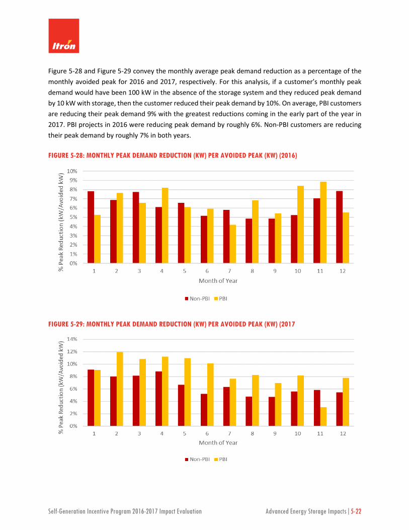
Self-Generation Incentive Program 2016-2017 Impact Evaluation Advanced Energy Storage Impacts|5-22
Figure 5-28 and Figure 5-29 convey the monthly average peak demand reduction as a percentage of the monthly avoided peak for 2016 and 2017, respectively. For this analysis, if a customer’s monthly peak demand would have been 100 kW in the absence of the storage system and they reduced peak demand by 10 kW with storage, then the customer reduced their peak demand by 10%. On average, PBI customers are reducing their peak demand 9% with the greatest reductions coming in the early part of the year in 2017. PBI projects in 2016 were reducing peak demand by roughly 6%. Non-PBI customers are reducing their peak demand by roughly 7% in both years.
FIGURE 5-28: MONTHLY PEAK DEMAND REDUCTION (KW) PER AVOIDED PEAK (KW) (2016)
FIGURE 5-29: MONTHLY PEAK DEMAND REDUCTION (KW) PER AVOIDED PEAK (KW) (2017
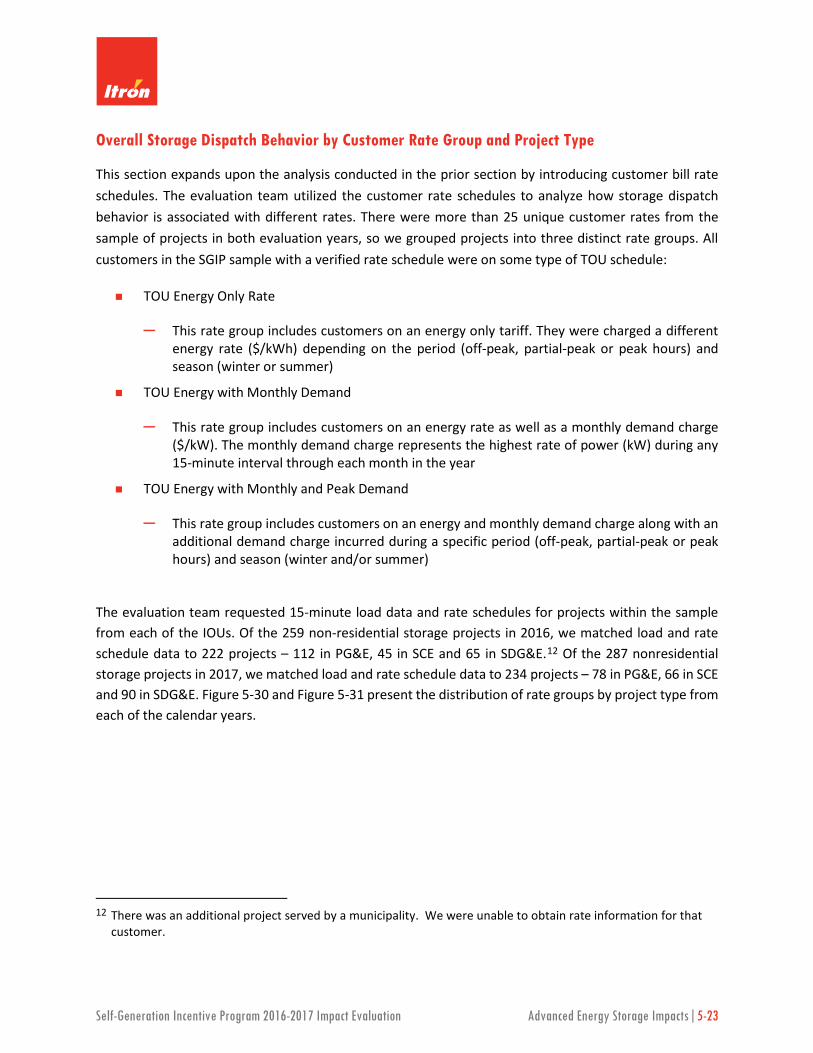
Self-Generation Incentive Program 2016-2017 Impact Evaluation Advanced Energy Storage Impacts|5-23
Overall Storage Dispatch Behavior by Customer Rate Group and Project Type
This section expands upon the analysis conducted in the prior section by introducing customer bill rate schedules. The evaluation team utilized the customer rate schedules to analyze how storage dispatch behavior is associated with different rates. There were more than 25 unique customer rates from the sample of projects in both evaluation years, so we grouped projects into three distinct rate groups. All customers in the SGIP sample with a verified rate schedule were on some type of TOU schedule:
TOU Energy Only Rate
─ This rate group includes customers on an energy only tariff. They were charged a different energy rate ($/kWh) depending on the period (off-peak, partial-peak or peak hours) and season (winter or summer)
TOU Energy with Monthly Demand
─ This rate group includes customers on an energy rate as well as a monthly demand charge ($/kW). The monthly demand charge represents the highest rate of power (kW) during any 15-minute interval through each month in the year
TOU Energy with Monthly and Peak Demand
─ This rate group includes customers on an energy and monthly demand charge along with an additional demand charge incurred during a specific period (off-peak, partial-peak or peak hours) and season (winter and/or summer)
The evaluation team requested 15-minute load data and rate schedules for projects within the sample from each of the IOUs. Of the 259 non-residential storage projects in 2016, we matched load and rate schedule data to 222 projects – 112 in PG&E, 45 in SCE and 65 in SDG&E.12 Of the 287 nonresidential storage projects in 2017, we matched load and rate schedule data to 234 projects – 78 in PG&E, 66 in SCE and 90 in SDG&E. Figure 5-30 and Figure 5-31 present the distribution of rate groups by project type from each of the calendar years.
12 There was an additional project served by a municipality. We were unable to obtain rate information for that
customer.
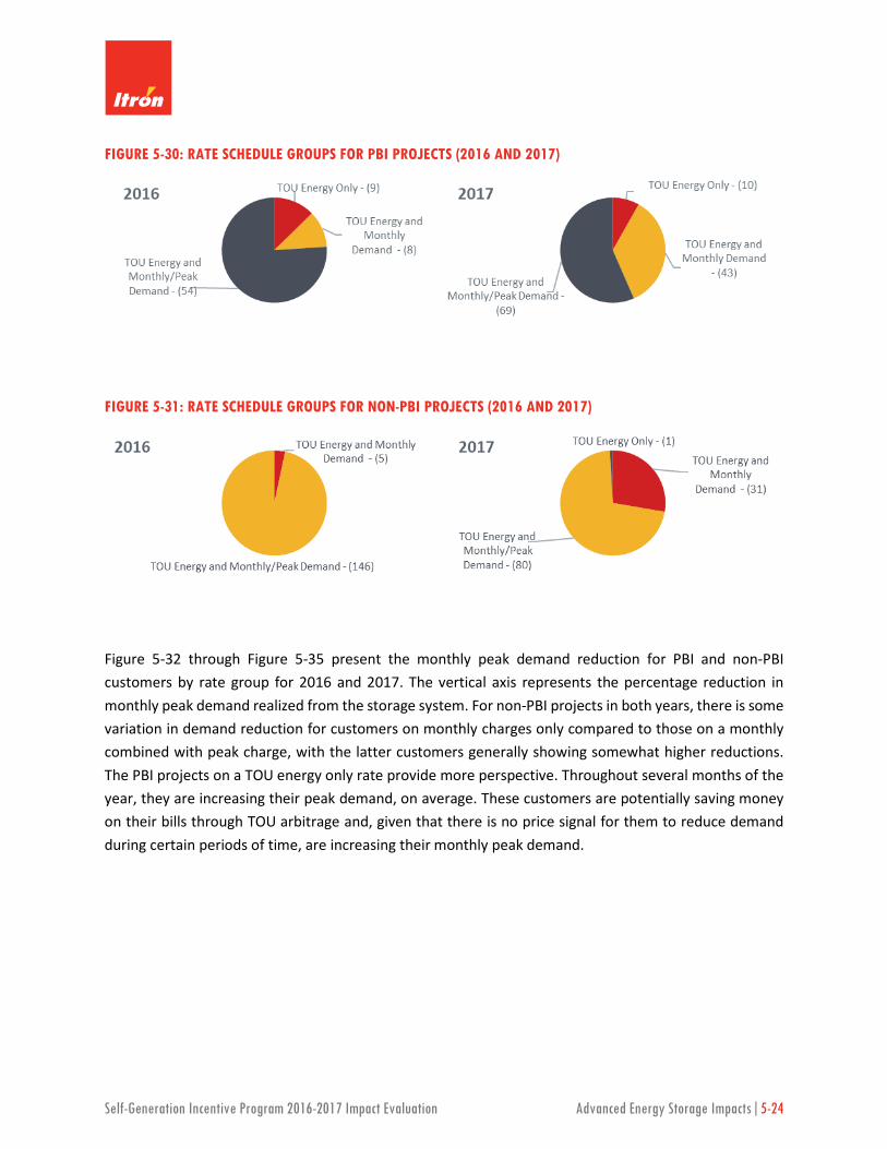
Self-Generation Incentive Program 2016-2017 Impact Evaluation Advanced Energy Storage Impacts|5-24
FIGURE 5-30: RATE SCHEDULE GROUPS FOR PBI PROJECTS (2016 AND 2017)
FIGURE 5-31: RATE SCHEDULE GROUPS FOR NON-PBI PROJECTS (2016 AND 2017)
Figure 5-32 through Figure 5-35 present the monthly peak demand reduction for PBI and non-PBI customers by rate group for 2016 and 2017. The vertical axis represents the percentage reduction in monthly peak demand realized from the storage system. For non-PBI projects in both years, there is some variation in demand reduction for customers on monthly charges only compared to those on a monthly combined with peak charge, with the latter customers generally showing somewhat higher reductions. The PBI projects on a TOU energy only rate provide more perspective. Throughout several months of the year, they are increasing their peak demand, on average. These customers are potentially saving money on their bills through TOU arbitrage and, given that there is no price signal for them to reduce demand during certain periods of time, are increasing their monthly peak demand.

Self-Generation Incentive Program 2016-2017 Impact Evaluation Advanced Energy Storage Impacts|5-25
FIGURE 5-32: PBI MONTHLY PEAK DEMAND REDUCTION (KW) PER AVOIDED PEAK (KW) BY RATE GROUP (2016)
FIGURE 5-33: PBI MONTHLY PEAK DEMAND REDUCTION (KW) PER AVOIDED PEAK (KW) BY RATE GROUP (2017)

Self-Generation Incentive Program 2016-2017 Impact Evaluation Advanced Energy Storage Impacts|5-26
FIGURE 5-34: NON-PBI MONTHLY PEAK DEMAND REDUCTION (KW) PER AVOIDED PEAK (KW) BY RATE GROUP (2016)
FIGURE 5-35: NON-PBI MONTHLY PEAK DEMAND REDUCTION (KW) PER AVOIDED PEAK (KW) BY RATE GROUP (2017)

Self-Generation Incentive Program 2016-2017 Impact Evaluation Advanced Energy Storage Impacts|5-27
Overall Customer Bill Savings ($/kW) by Rate Group and Project Type
Finally, we combined the energy rates charged during each of the TOU periods and compared energy consumption with storage versus calculated energy consumption in the absence of storage to develop bill impact estimates for customers. For customers with demand charges, we further estimated the reduction (or increase) in peak demand on a monthly level and during specific TOU periods and calculated demand savings (or costs) based on the specific customer rate schedule. The expectation is that customers on a TOU energy only rate are discharging during periods when energy rates are high and charging during periods of lower prices which would translate into bill savings. For customers with demand charges, the expectation is that they are optimizing either monthly facility demand charge reduction or peak period demand charge reduction, perhaps, at the expense of TOU energy arbitrage. Figure 5-36 and Figure 5-37 on the following page present those results for PBI and non-PBI projects by rate group for 2016 and 2017. The vertical axis represents the average monthly savings (or cost) in dollars, normalized by rebated capacity.
For both non-PBI rate groups, customers incurred energy costs, on average, by utilizing their storage systems. Both the monthly demand and the monthly demand with peak groups realized significant savings by optimizing their storage to reduce peak and/or monthly demand. PBI projects on a TOU energy only rate realized energy savings from the storage systems which suggests they were optimizing dispatch for TOU arbitrage. PBI customers with demand charges realized savings from demand reduction, while energy charges had a negligible effect on their bill.

Self-Generation Incentive Program 2016-2017 Impact Evaluation Advanced Energy Storage Impacts|5-28
FIGURE 5-36: CUSTOMER BILL SAVINGS ($/KW) BY RATE GROUP AND PBI/NON-PBI (2016)
FIGURE 5-37: CUSTOMER BILL SAVINGS ($/KW) BY RATE GROUP AND PBI/NON-PBI (2017)

Self-Generation Incentive Program 2016-2017 Impact Evaluation Advanced Energy Storage Impacts|5-29
5.2.2 Residential Projects
For the 28 projects for which data are available in 2017, we’ve conducted a high-level assessment of how residential storage systems are being utilized throughout the day and year. Figure 5-38 and Figure 5-39 convey those findings. These projects generally discharge from late morning starting at 11 am until midafternoon at about 4 pm. They are consistently charging directly after this period, from 4 pm until midnight.
FIGURE 5-38: AVERAGE HOURLY DISCHARGE (KW) PER REBATED CAPACITY (KW) FOR RESIDENTIAL PROJECTS
Jan Feb Mar Apr May Jun Jul Aug Sep Oct Nov Dec1 2 3 4 5 6 7 8 9 10 11 12
0 0.000 0.000 0.000 0.000 0.000 0.000 0.000 0.000 0.000 0.000 0.000 0.0001 0.001 0.000 0.000 0.000 0.000 0.000 0.000 0.000 0.000 0.000 0.000 0.0002 0.000 0.000 0.000 0.000 0.000 0.000 0.000 0.000 0.000 0.000 0.000 0.0003 0.000 0.000 0.000 0.000 0.000 0.000 0.000 0.000 0.000 0.000 0.000 0.0004 0.001 0.000 0.000 0.000 0.000 0.000 0.000 0.000 0.000 0.000 0.000 0.0005 0.001 0.000 0.000 0.000 0.000 0.000 0.000 0.000 0.000 0.000 0.000 0.0006 0.001 0.000 0.000 0.000 0.000 0.000 0.000 0.000 0.000 0.000 0.000 0.0007 0.000 0.000 0.000 0.000 0.000 0.000 0.000 0.000 0.000 0.000 0.000 0.0008 0.001 0.000 0.000 0.000 0.000 0.000 0.000 0.000 0.000 0.000 0.000 0.0009 0.000 0.000 0.000 0.000 0.000 0.000 0.000 0.000 0.000 0.000 0.000 0.00010 0.000 0.000 0.000 0.000 0.000 0.001 0.000 0.000 0.000 0.000 0.000 0.00011 0.053 0.053 0.049 0.041 0.046 0.053 0.036 0.038 0.047 0.081 0.139 0.15812 0.052 0.052 0.046 0.066 0.072 0.078 0.060 0.063 0.059 0.087 0.139 0.15813 0.052 0.050 0.046 0.065 0.073 0.077 0.060 0.062 0.053 0.035 0.022 0.05514 0.052 0.050 0.046 0.067 0.075 0.079 0.062 0.063 0.053 0.034 0.017 0.05415 0.034 0.040 0.039 0.063 0.066 0.070 0.057 0.055 0.040 0.028 0.016 0.04416 0.000 0.000 0.000 0.000 0.000 0.000 0.000 0.000 0.000 0.009 0.012 0.04017 0.000 0.000 0.000 0.000 0.000 0.000 0.000 0.000 0.000 0.000 0.000 0.00018 0.000 0.000 0.000 0.000 0.000 0.000 0.000 0.000 0.000 0.000 0.000 0.00019 0.001 0.000 0.000 0.000 0.000 0.000 0.000 0.000 0.000 0.000 0.000 0.00020 0.001 0.000 0.000 0.000 0.000 0.000 0.000 0.000 0.000 0.000 0.000 0.00021 0.001 0.000 0.000 0.000 0.000 0.000 0.000 0.000 0.000 0.000 0.000 0.00022 0.000 0.000 0.000 0.000 0.000 0.000 0.000 0.000 0.000 0.000 0.000 0.00023 0.000 0.000 0.000 0.000 0.000 0.000 0.000 0.000 0.000 0.000 0.000 0.000
Hour

Self-Generation Incentive Program 2016-2017 Impact Evaluation Advanced Energy Storage Impacts|5-30
FIGURE 5-39: AVERAGE CHARGE (KW) PER REBATED CAPACITY (KW) FOR RESIDENTIAL PROJECTS
5.3 CAISO AND IOU SYSTEM IMPACTS
The timing and magnitude of storage dispatch throughout the year can also have an impact on the electricity grid. As detailed above, SGIP storage projects are generally being utilized to reduce non-coincident monthly peak demand and, to a lesser extent, TOU energy arbitrage. Benefits that may accrue to the CAISO or IOU system are potentially due to participation in demand response programs (both system-level/localized and real-time/day-ahead), enrollment in IOU tariffs which include peak energy pricing like Critical Peak Pricing (CPP) or Peak Day Pricing (PDP) or are just merely coincidental. Storage project operators and host customers may not be aware of system or utility level peak hours unless they are enrolled in a demand response program or retail rate, where a price signal is generated to shift or reduce demand. Customers understand their facility operations and bill rate structure, but grid level demand may not be in their purview.
Storage discharge behavior that is coincident with critical system hours can provide additional benefits beyond customer-specific ones. These benefits include avoided generation capacity costs and transmission and distribution costs. The evaluation team assessed this potential benefit by quantifying
Jan Feb Mar Apr May Jun Jul Aug Sep Oct Nov Dec1 2 3 4 5 6 7 8 9 10 11 12
0 -0.007 -0.010 -0.013 -0.012 -0.012 -0.010 -0.010 -0.010 -0.009 -0.008 -0.006 -0.0071 -0.007 -0.009 -0.011 -0.010 -0.010 -0.009 -0.011 -0.009 -0.008 -0.008 -0.007 -0.0062 -0.007 -0.009 -0.011 -0.009 -0.010 -0.009 -0.010 -0.009 -0.008 -0.009 -0.007 -0.0073 -0.006 -0.010 -0.010 -0.008 -0.009 -0.009 -0.009 -0.008 -0.010 -0.009 -0.007 -0.0074 -0.006 -0.009 -0.009 -0.009 -0.009 -0.009 -0.008 -0.009 -0.008 -0.008 -0.007 -0.0075 -0.005 -0.007 -0.009 -0.009 -0.009 -0.010 -0.009 -0.010 -0.008 -0.009 -0.007 -0.0086 -0.005 -0.008 -0.010 -0.010 -0.010 -0.011 -0.009 -0.010 -0.011 -0.009 -0.008 -0.0077 -0.007 -0.009 -0.010 -0.010 -0.011 -0.011 -0.009 -0.010 -0.010 -0.009 -0.008 -0.0078 -0.007 -0.008 -0.009 -0.009 -0.009 -0.010 -0.009 -0.011 -0.008 -0.010 -0.007 -0.0079 -0.006 -0.008 -0.010 -0.009 -0.009 -0.009 -0.009 -0.010 -0.009 -0.010 -0.008 -0.00710 -0.006 -0.008 -0.009 -0.009 -0.010 -0.010 -0.010 -0.009 -0.009 -0.009 -0.007 -0.00811 -0.005 -0.006 -0.008 -0.008 -0.009 -0.008 -0.008 -0.008 -0.007 -0.005 -0.003 -0.00112 -0.004 -0.006 -0.009 -0.008 -0.008 -0.008 -0.009 -0.007 -0.006 -0.006 -0.003 -0.00113 -0.005 -0.007 -0.008 -0.008 -0.007 -0.008 -0.010 -0.008 -0.010 -0.028 -0.053 -0.04514 -0.005 -0.006 -0.008 -0.008 -0.007 -0.008 -0.009 -0.008 -0.015 -0.060 -0.129 -0.11015 -0.006 -0.007 -0.010 -0.008 -0.008 -0.010 -0.009 -0.011 -0.021 -0.064 -0.133 -0.11516 -0.046 -0.047 -0.048 -0.050 -0.054 -0.061 -0.046 -0.045 -0.049 -0.038 -0.038 -0.04317 -0.044 -0.047 -0.045 -0.055 -0.060 -0.064 -0.051 -0.052 -0.051 -0.033 -0.019 -0.03718 -0.043 -0.044 -0.042 -0.054 -0.060 -0.064 -0.051 -0.052 -0.050 -0.038 -0.023 -0.06319 -0.042 -0.044 -0.041 -0.060 -0.063 -0.070 -0.058 -0.061 -0.057 -0.052 -0.040 -0.09420 -0.041 -0.044 -0.042 -0.060 -0.066 -0.069 -0.054 -0.052 -0.042 -0.039 -0.033 -0.07821 -0.040 -0.043 -0.043 -0.059 -0.065 -0.069 -0.054 -0.054 -0.041 -0.036 -0.030 -0.07422 -0.038 -0.041 -0.039 -0.051 -0.058 -0.058 -0.048 -0.049 -0.041 -0.032 -0.025 -0.06123 -0.021 -0.027 -0.026 -0.039 -0.036 -0.033 -0.029 -0.029 -0.022 -0.015 -0.009 -0.011
Hour

Self-Generation Incentive Program 2016-2017 Impact Evaluation Advanced Energy Storage Impacts|5-31
the storage dispatch from our sample of nonresidential and residential projects throughout the top 200 peak demand hours in 2016 and 2017 for both the CAISO system13 as well as the three IOUs.
5.3.1 Non-Residential System Impacts
Figure 5-40 and Figure 5-41 below present the average kW discharge per rebated capacity for non-PBI projects along with the peak MW for each of the top 200 CAISO hours in 2016 and 2017, respectively. Non-PBI projects were charging during most top CAISO hours in both years and the magnitude of impact is similar across years.
FIGURE 5-40: AVERAGE HOURLY NET DISCHARGE KW PER KW DURING CAISO TOP 200 HOURS FOR NON-PBI PROJECTS (2016)
13 The top 200 CAISO peak hours all fall within June and September. In 2016, the top CAISO load hour was on 7/27
at 3 pm (PST). The top CAISO load hour in 2017 was on 9/1 at 3 pm (PST). The top 5 CAISO load hours occurred on that day (1 pm through 5 pm).

Self-Generation Incentive Program 2016-2017 Impact Evaluation Advanced Energy Storage Impacts|5-32
FIGURE 5-41: AVERAGE HOURLY NET DISCHARGE KW PER KW DURING CAISO TOP 200 HOURS FOR NON-PBI PROJECTS (2017)
Figure 5-42 and Figure 5-43 present the average kW discharge per rebated capacity for PBI projects along with the peak MW for each of the top 200 CAISO hours in 2016 and 2017, respectively. PBI projects were discharging throughout the majority of CAISO peak hours in both years. Results for 2017 are less consistent with findings from 2016 in terms of the magnitude of average net discharge kW throughout the top 200 hours.

Self-Generation Incentive Program 2016-2017 Impact Evaluation Advanced Energy Storage Impacts|5-33
FIGURE 5-42 AVERAGE HOURLY NET DISCHARGE KW PER KW DURING CAISO TOP 200 HOURS FOR PBI PROJECTS (2016)
FIGURE 5-43: AVERAGE HOURLY NET DISCHARGE KW PER KW DURING CAISO TOP 200 HOURS FOR PBI PROJECTS (2017)

Self-Generation Incentive Program 2016-2017 Impact Evaluation Advanced Energy Storage Impacts|5-34
While the peak CAISO load hours differ across years, the makeup of the PBI population has also changed considerably since 2016. In 2016, the top 200 CAISO hours occurred prior to October. Sixteen projects received their upfront payment in the final three months of that year. Furthermore, 62 additional projects received upfront payments in 2017 and were not subject to evaluation in 2016. Of those 78 total projects, 34 are primary and secondary schools.
Figure 5-44 presents the average storage discharge profiles of four facility types on September 1, 2017. The five top CAISO hours occurred within that day from 1 pm throughout 5 pm (PST) and are highlighted in light blue. The CAISO load profile is also overlaid in the figure. These facility types include (clockwise from top left), industrial facilities, schools, offices and retail establishments and represent 43%, 18%, 9% and 7%, respectively – or collectively, 77% – of the total 2017 rebated capacity for PBI projects. Schools are the only facility type, on average, charging throughout the top 5 CAISO hours. These systems were presumably discharging throughout the morning ramp period to satisfy non-coincident facility demand and charged throughout the afternoon period to maintain a balanced state of charge.
FIGURE 5-44: STORAGE DISCHARGE KW ON SEPTEMBER 1, 2017

Self-Generation Incentive Program 2016-2017 Impact Evaluation Advanced Energy Storage Impacts|5-35
We also examined the net discharge behavior of storage systems for peak IOU load hours. The results are presented below in Figure 5-45 through Figure 5-48. The results are much like those on the CAISO peak hours. PBI projects, on average, are discharging during system peak hours and non-PBI projects, on average, are charging during those hours. Again, this could be explained by the fact that non-PBI customers are optimizing storage dispatch for noncoincident peak demand reduction. They are smaller systems that exhibit a “snap-back” effect where discharge events are immediately followed by a charge event. Larger storage systems exhibit discharge behavior, often followed by an idle period. Charging does not occur until later in the evening or overnight.
One striking difference across utility top peak loads throughout 2017 is the average net charge of PBI storage systems operating in SDG&E territory. As presented above in Figure 5-44, schools were generally charging throughout CAISO peak hours (many of which were coincident with SDG&E system load) after discharging throughout the morning hours. Of the 43 PBI school storage systems, 21 were operating within SDG&E’s service territory in 2017. These systems combined represent 6.4 MW of rebated capacity or roughly 50% of the total rebated capacity for PBI systems operating in SDG&E territory. These projects received their upfront payment in 2017 and were not subject to evaluation in 2016.
FIGURE 5-45: NET DISCHARGE KWH PER REBATED CAPACITY KW DURING SYSTEM PEAK HOURS FOR PBI PROJECTS (2016)

Self-Generation Incentive Program 2016-2017 Impact Evaluation Advanced Energy Storage Impacts|5-36
FIGURE 5-46: NET DISCHARGE KWH PER REBATED CAPACITY KW DURING SYSTEM PEAK HOURS FOR PBI PROJECTS (2017)
FIGURE 5-47: NET DISCHARGE KWH PER REBATED CAPACITY KW DURING SYSTEM PEAK HOURS FOR NON-PBI PROJECTS (2016)

Self-Generation Incentive Program 2016-2017 Impact Evaluation Advanced Energy Storage Impacts|5-37
FIGURE 5-48: NET DISCHARGE KWH PER REBATED CAPACITY KW DURING SYSTEM PEAK HOURS FOR NON-PBI PROJECTS (2017)
5.3.2 Residential System Impacts
Figure 5-49 on the following page presents the average kW discharge per rebated capacity for residential projects along with the peak MW for each of the top 200 CAISO hours. The pattern of charge and discharge of residential storage systems is far less consistent than nonresidential projects. During summer months (which coincide with the CAISO peak hours), the sample of residential projects were either mostly idle or cycling throughout the daytime hours (Figure 5-8).
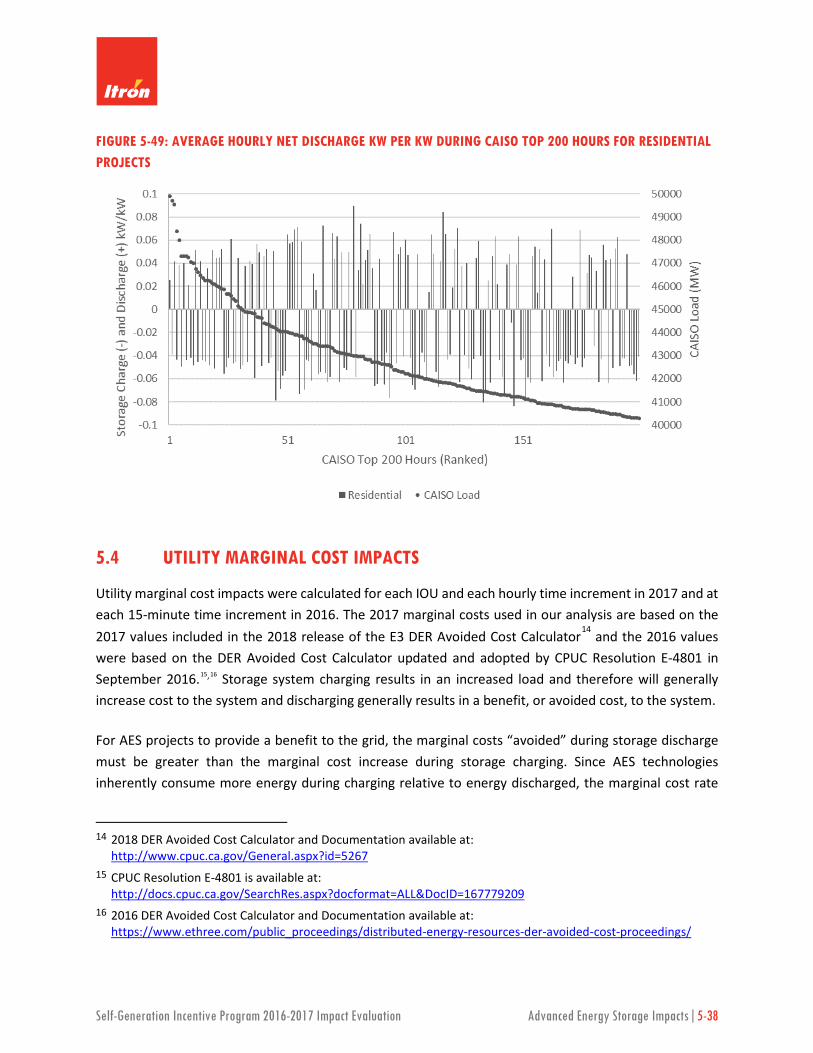
Self-Generation Incentive Program 2016-2017 Impact Evaluation Advanced Energy Storage Impacts|5-38
FIGURE 5-49: AVERAGE HOURLY NET DISCHARGE KW PER KW DURING CAISO TOP 200 HOURS FOR RESIDENTIAL PROJECTS
5.4 UTILITY MARGINAL COST IMPACTS
Utility marginal cost impacts were calculated for each IOU and each hourly time increment in 2017 and at each 15-minute time increment in 2016. The 2017 marginal costs used in our analysis are based on the 2017 values included in the 2018 release of the E3 DER Avoided Cost Calculator14 and the 2016 values were based on the DER Avoided Cost Calculator updated and adopted by CPUC Resolution E-4801 in September 2016.15,16 Storage system charging results in an increased load and therefore will generally increase cost to the system and discharging generally results in a benefit, or avoided cost, to the system.
For AES projects to provide a benefit to the grid, the marginal costs “avoided” during storage discharge must be greater than the marginal cost increase during storage charging. Since AES technologies inherently consume more energy during charging relative to energy discharged, the marginal cost rate
14 2018 DER Avoided Cost Calculator and Documentation available at:
http://www.cpuc.ca.gov/General.aspx?id=5267 15 CPUC Resolution E-4801 is available at:
http://docs.cpuc.ca.gov/SearchRes.aspx?docformat=ALL&DocID=167779209 16 2016 DER Avoided Cost Calculator and Documentation available at:
https://www.ethree.com/public_proceedings/distributed-energy-resources-der-avoided-cost-proceedings/

Self-Generation Incentive Program 2016-2017 Impact Evaluation Advanced Energy Storage Impacts|5-39
must be lower during charging hours relative to discharge hours. In other words, SGIP storage projects that charge during lower marginal cost periods and discharge during higher marginal cost periods will provide a net benefit to the system. The avoided costs that were included in this analysis include energy, system capacity, renewable portfolio standard (RPS), ancillary services ($/kWh) costs and distribution and transmission.17 It is important to note that system operators are generally not aware of the cost of generating, transporting and supplying energy.
5.4.1 Non-Residential Projects
The normalized utility marginal costs for 2016 and 2017 are shown in Figure 5-50 and Figure 5-51 by electric IOU and project type (non-PBI and PBI). Marginal avoided costs are positive (+) and marginal incurred costs are negative (-).
FIGURE 5-50: MARGINAL COST $ PER REBATED CAPACITY (KW) BY IOU AND PROJECT TYPE (2016)
17 The 2016 evaluation did not include the marginal costs associated with distribution.

Self-Generation Incentive Program 2016-2017 Impact Evaluation Advanced Energy Storage Impacts|5-40
FIGURE 5-51: MARGINAL COST $ PER REBATED CAPACITY (KW) BY IOU AND PROJECT TYPE (2017)
Overall, non-PBI projects represent a net cost to the utility system per rebated capacity. The marginal costs modeled in this study are highest when energy prices are high and the CAISO system load is peaking. Non-PBI projects are net charging, on average, throughout the year. In other words, these projects are charging during both low and high marginal cost periods. These projects were also charging during CAISO peak hours which represents a net capacity cost. PBI projects, conversely, are providing a net marginal benefit for two utilities in both 2016 and 2017. These projects were generally discharging during periods when energy prices were high and charging overnight, when marginal prices were lower. The benefits generated during the discharge periods are greater than the cost incurred during storage charge. Likewise, PBI systems were generally discharging during peak CAISO hours. This provides a significant capacity benefit.
5.4.2 Residential Projects
The normalized utility marginal costs are shown in Figure 5-52 for residential projects by electric IOU in 2017. Marginal avoided costs are positive (+) and marginal incurred costs are negative (-). The average marginal cost (-) for residential projects is $10.86 per rebated capacity (kW).

Self-Generation Incentive Program 2016-2017 Impact Evaluation Advanced Energy Storage Impacts|5-41
FIGURE 5-52: MARGINAL COST $ PER REBATED CAPACITY (KW) BY IOU (RESIDENTIAL PROJECTS) (2017)
5.5 POPULATION IMPACTS
Metered data available for the sample of projects were used to estimate population total impacts for both 2016 and 2017. Relative precision levels reported in the tables are based on a confidence level of 90%. Population estimates were calculated for the following impacts:
Customer average summer-time peak demand
CAISO system peak demand (top hour and top 200 hours)
Electric energy
Customer peak demand impacts during summer months provide some indication of the way nonresidential customers are utilizing their AES systems to manage loads and reduce electricity costs. Summarizing these impacts of SGIP AES systems is complicated by the fact that projects are coming online periodically throughout the year, and tariff definitions of ‘summer’ vary. Consequently, a simplified measure of average monthly population total customer peak demand impacts was calculated. For each customer, the impact of AES on billed demand for each of four summer months (June through September) was calculated as the difference between observed maximum 15-minute net load and an estimate of the load that would have been observed without the AES. Results calculated for each of those four summer months were averaged for each sampled participant. Finally, estimated impacts for the entire population were approximated based on the total number of complete projects at the end of July. Summer-time average customer peak demand impacts are summarized in Table 5-1. PBI and non-PBI nonresidential

Self-Generation Incentive Program 2016-2017 Impact Evaluation Advanced Energy Storage Impacts|5-42
projects produced reductions in summertime average customer peak demand in both 2016 and 2017. Residential projects increased peak demand slightly in 2017.
TABLE 5-1: POPULATION TOTAL SUMMER-TIME AVERAGE CUSTOMER PEAK DEMAND IMPACTS
Year Customer Sector N Population Impact (kW) Relative Precision
2016 Nonresidential PBI 69 -1,435 8% Nonresidential Non-PBI 240 -484 8% Total 309 -1,919 6%
2017
Nonresidential PBI 138 -1,918 3% Nonresidential Non-PBI 275 -496 8% Residential 400 28 18% Total 813 -2,386 3%
CAISO system peak demand impacts are summarized in Table 5-2 (top hour). In 2016, the CAISO statewide system load peaked at 45,981 MW on July 27 during the hour from 3 to 4 PM PST and in 2017, peaked at 49,909 MW on September 1 during the hour from 3 to 4 PM PST. While PBI projects delivered CAISO system peak demand reduction exceeding 8.8 MW in 2016 and 4 MW in 2017, non-PBI nonresidential projects were net consumers of electricity during this hour. On average, the non-PBI projects were charging during the hour of the CAISO system peak whereas the PBI projects were discharging. The poor relative precision reported for non-PBI (both residential and nonresidential) is largely a consequence of the small population estimate of total impacts and variability in project-specific storage dispatch behavior throughout the CAISO top hour.
TABLE 5-2: CAISO SYSTEM PEAK DEMAND IMPACTS (PEAK HOUR)
Year Customer Sector N Population Impact (kW) Relative Precision
2016 Nonresidential PBI 69 -8,848 8% Nonresidential Non-PBI 240 69 82% Total 309 -8,779 8%
2017
Nonresidential PBI 139 -4,002 13% Nonresidential Non-PBI 278 420 49% Residential 405 -53 141% Total 822 -3,635 15%

Self-Generation Incentive Program 2016-2017 Impact Evaluation Advanced Energy Storage Impacts|5-43
TABLE 5-3: CAISO SYSTEM PEAK DEMAND IMPACTS (TOP 200 HOURS)
Year Customer Sector N Population Impact (kW) Relative Precision
2016 Nonresidential PBI 76 -5,544 3% Nonresidential Non-PBI 242 127 11% Total 318 -5,416 3%
2017
Nonresidential PBI 139 -2,942 9% Nonresidential Non-PBI 278 200 13% Residential 405 14 79% Total 822 -2,728 9%
Electric energy impacts (i.e., the total energy impact that resulted from charging and discharging AES projects) during 2016 and 2017 are summarized in Table 5-4. Electric energy impacts for both PBI and non-PBI are positive, reflecting increased energy consumption, as expected. This summary result reflects the combined effects of several factors, including timing of charging and discharging, standby loss rates and utilization levels and roundtrip efficiency. The total energy impact was an increase in electric energy consumption of 5,579 MWh during 2017 and 4,672 MWh in 2016.
TABLE 5-4: ELECTRIC ENERGY IMPACTS
Year Customer Sector N Population Impact (MWh) Relative Precision
2016 Nonresidential PBI 83 3,692 2% Nonresidential Non-PBI 246 980 5% Total 329 4,672 2%
2017
Nonresidential PBI 143 4,339 2% Nonresidential Non-PBI 278 1,041 10% Residential 407 198 8% Total 828 5,579 3%
Utility marginal cost impacts during 2016 and 2017 are summarized in Table 5-5. Utility marginal costs are negative for PBI projects (costs were avoided) and positive for non-PBI residential and nonresidential projects (costs were incurred).

Self-Generation Incentive Program 2016-2017 Impact Evaluation Advanced Energy Storage Impacts|5-44
TABLE 5-5: UTILITY MARGINAL COST IMPACTS
Year Customer Sector N Population Impact (Avoided Cost $) Relative Precision
2016 Nonresidential PBI 83 ($86,384) 10% Nonresidential Non-PBI 246 $43,356 6% Total 329 ($43,029) 21%
2017
Nonresidential PBI 143 ($646,693) 10% Nonresidential Non-PBI 278 $144,719 17% Residential 407 $22,972 28% Total 828 ($479,002) 14%

Self-Generation Incentive Program 2016-2017 Impact Evaluation Environmental Impacts|6-1
6 ENVIRONMENTAL IMPACTS The Self-Generation Incentive Program (SGIP) was originally established in 2001 to help address California’s peak electricity supply shortcomings. Projects rebated by the SGIP were designed to maximize electricity generation during utility system peak periods and not necessarily to reduce greenhouse gas (GHG) or criteria air pollutant emissions. Passage of Senate Bill (SB) 412 (Kehoe) required the California Public Utilities Commission (CPUC) to establish GHG goals for the SGIP.
This section discusses the GHG and criteria air pollutant impacts of the SGIP during calendar years 2016 and 2017. The fleet of projects whose impacts are evaluated in this section includes projects completed before the passage of SB 412. The GHG impact analysis is limited to carbon dioxide (CO2) and CO2 equivalent (CO2eq) methane (CH4) emissions impacts associated with SGIP projects. The criteria air pollutant impact analysis is limited to NOX and PM10 emissions impacts associated with SGIP projects. The discussion is organized into the following subsections:
Methodology Overview and Summary of Environmental Impacts
Non-renewable Generation Project Impacts
Renewable Biogas Generation Project Impacts
Wind and Pressure Reduction Turbine (PRT) Project Impacts
Advanced Energy Storage (AES) Project Impacts
The scope of this analysis is further limited to operational impacts of SGIP projects and does not discuss any lifecycle emissions impacts that occur during the manufacturing, transportation, and construction of SGIP projects. A more detailed discussion of the environmental impacts methodology is included in Appendix C and Appendix D.
6.1 BACKGROUND AND BASELINE DISCUSSION
Emission impacts are calculated as the difference between the emissions generated by SGIP projects and baseline emissions that would have occurred in the absence of the program. The sources of these emissions (generated and avoided) vary by technology and fuel type. For example, all distributed generation technologies avoid emissions associated with displacing central station grid electricity, but only those that recover useful heat avoid emissions associated with displacing boiler use.

Self-Generation Incentive Program 2016-2017 Impact Evaluation Environmental Impacts|6-2
6.1.1 Grid Electricity Baseline
The passage of SB 412 established a maximum GHG emissions rate for SGIP generation technologies. Beginning in 2011, eligibility for SGIP generation projects was limited to projects that did not exceed an emissions rate of 379 kg CO2/MWh over ten years. Later, the CPUC revised the maximum GHG emission rate for eligibility to 350 kg CO2/MWh over ten years for projects applying to the SGIP in 2016.
When developing these emission factors for eligibility, the CPUC must look forward and forecast what baseline grid conditions will look like during an SGIP project’s life. These forecasts must make assumptions about power plant efficiencies and the useful life of SGIP projects. By contrast, an impact evaluation has the benefit of being backwards looking and is able to leverage historical data to quantify the grid electricity baseline.
Consequently, the avoided grid emissions rates used in this impact evaluation report to assess project performance are different than the avoided grid emissions factors used to screen SGIP applications for program eligibility requirements. This evaluation relies on avoided grid emissions rates calculated using the latest version of the CPUC’s Avoided Cost Calculator (ACC).1
6.1.2 Greenhouse Gas Impact Summary
Overall, the SGIP reduced GHG emissions by almost 155 thousand metric tons of CO2eq during 2016, and by almost 160 thousand metric tons of CO2eq during 2017. For 2016, this is equivalent to a rate of 314 metric tons of CO2eq reduced per rebated MW, and 287 metric tons of CO2eq per rebated MW for 2017.
Figure 6-1 shows the GHG impacts of the eight technology types rebated by the SGIP, including both generation and energy storage. The impacts shown in Figure 6-1 represent program level impacts for all fuel types (renewable and non-renewable). However, the environmental impacts for renewable and non-renewable projects vary greatly for any given technology. Detailed breakdowns of environmental impacts by technology and fuel type are provided in subsequent figures and tables.
Electric-only fuel cells achieved the largest reductions in GHG emissions during both 2016 and 2017, followed by IC engines during both years. Gas turbines, microturbines, and AES all showed a positive GHG emissions impact, indicating that these SGIP technologies emitted greater GHG emissions than their conventional baselines. Subsequent sections will explore potential reasons for the observed GHG impacts.
1 http://www.cpuc.ca.gov/General.aspx?id=5267

Self-Generation Incentive Program 2016-2017 Impact Evaluation Environmental Impacts|6-3
FIGURE 6-1: GREENHOUSE GAS IMPACTS BY TECHNOLOGY TYPE AND CALENDAR YEAR
Figure 6-2 below shows the GHG impacts of the program in 2016 and 2017 by their fuel energy source. Renewable biogas fueled technologies (both on-site and directed), along with technologies with no fuel input (e.g., AES, wind and pressure reduction turbines) reduced GHG emissions on average. Non-renewable generation technologies increased emissions across both years on average. However not all non-renewable technologies led to increased GHG emissions. Subsequent sections will explore each fuel type in detail. Non-renewable fueled projects saw a reduction in GHG emissions in 2017, driven by two factors. The first was the performance of non-renewable IC engines. IC engines saw reduced GHG emissions in 2017, as seen in Figure 6-7 below. The second factor had to do with electric-only fuel cells. There were about 50 new non-renewable electric-only fuel cells which came online in 2017, which reduced overall GHG emissions. These two factors combined provided the large increase in 2017 GHG reductions for non-renewable fueled projects.
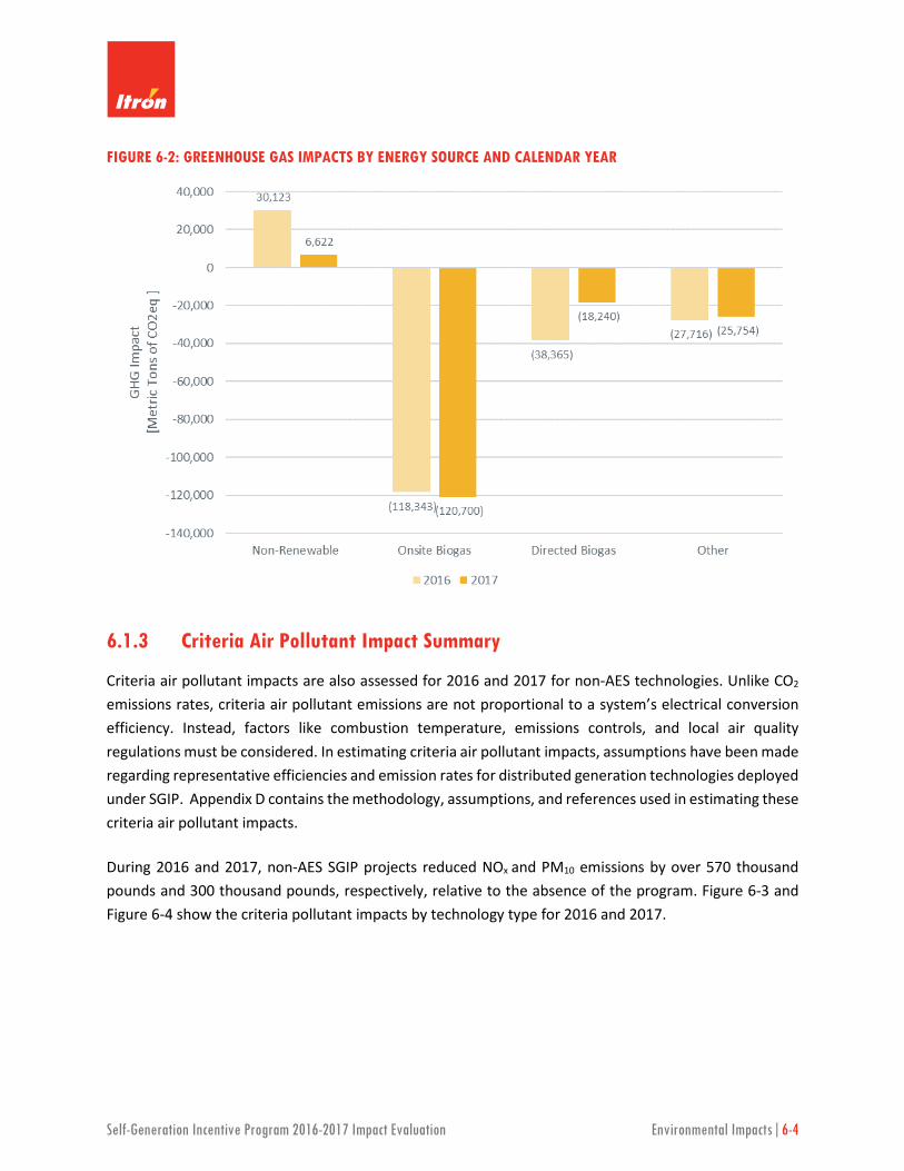
Self-Generation Incentive Program 2016-2017 Impact Evaluation Environmental Impacts|6-4
FIGURE 6-2: GREENHOUSE GAS IMPACTS BY ENERGY SOURCE AND CALENDAR YEAR
6.1.3 Criteria Air Pollutant Impact Summary
Criteria air pollutant impacts are also assessed for 2016 and 2017 for non-AES technologies. Unlike CO2 emissions rates, criteria air pollutant emissions are not proportional to a system’s electrical conversion efficiency. Instead, factors like combustion temperature, emissions controls, and local air quality regulations must be considered. In estimating criteria air pollutant impacts, assumptions have been made regarding representative efficiencies and emission rates for distributed generation technologies deployed under SGIP. Appendix D contains the methodology, assumptions, and references used in estimating these criteria air pollutant impacts.
During 2016 and 2017, non-AES SGIP projects reduced NOx and PM10 emissions by over 570 thousand pounds and 300 thousand pounds, respectively, relative to the absence of the program. Figure 6-3 and Figure 6-4 show the criteria pollutant impacts by technology type for 2016 and 2017.

Self-Generation Incentive Program 2016-2017 Impact Evaluation Environmental Impacts|6-5
FIGURE 6-3: CRITERIA POLLUTANT IMPACTS BY TECHNOLOGY TYPE (2016)
* Criteria air pollutant impacts were not evaluated in 2016 for AES technologies.
FIGURE 6-4: CRITERIA POLLUTANT IMPACTS BY TECHNOLOGY TYPE (2017)

Self-Generation Incentive Program 2016-2017 Impact Evaluation Environmental Impacts|6-6
Figure 6-5 shows the criteria pollutant impacts by energy source. Non-renewable sources demonstrated the largest reduction in NOx and PM emissions, with over 320 thousand pounds and 230 thousand pounds respectively.
FIGURE 6-5: CRITERIA POLLUTANT IMPACTS BY ENERGY SOURCE (2016 AND 2017)
6.2 NON-RENEWABLE GENERATION PROJECT IMPACTS
SGIP non-renewable generation projects include fuel cells (CHP and electric-only), gas turbines, IC engines, and microturbines. These projects are powered by natural gas and used to generate electricity to serve a customer’s load. These projects produce emissions that are proportional to the amount of fuel they consume. In the absence of the program, the customer’s electrical load would have been served by the electricity distribution company. Consequently, if SGIP projects only served electrical loads, they would need to generate electricity more cleanly than the avoided marginal grid generator to achieve GHG emission reductions.
SGIP CHP projects recover waste heat and use it to serve on-site thermal loads, like a customer’s heating or cooling needs. In the absence of the SGIP, a heating end use is assumed to be met by a natural gas

Self-Generation Incentive Program 2016-2017 Impact Evaluation Environmental Impacts|6-7
boiler, and the cooling end-use met with an electric chiller. Natural gas boilers generate emissions associated with the combustion of gas to heat water. The emissions associated with electric chillers are due to the central station plant that would have generated the electricity to run the chiller. Emissions impacts are the difference between the SGIP emissions and those avoided emissions.
6.2.1 Non-renewable Generation Project Greenhouse Gas Impacts
The GHG impact rates of non-renewable SGIP generation projects are shown below in Figure 6-6. Fuel cell technologies (both CHP and electric-only) demonstrated a reduction in greenhouse gas impacts, while combustion technologies increased the amount of GHG emissions over their assumed baseline. Microturbines were found to have the highest impact rates on a metric ton of CO2 per MWh generated basis than other technologies, at 0.29 and 0.36 for 2016 and 2017 respectively. IC engines in 2016 also saw high rates of 0.26 metric tons of CO2eq per MWh generated, but dropped significantly in 2017.
FIGURE 6-6: NON-RENEWABLE GREENHOUSE GAS IMPACT RATE BY TECHNOLOGY TYPE AND CALENDAR YEAR
While the impact rates displayed above in Figure 6-6, and below in Table 6-1 and Table 6-2 show that at a technology level, non-renewable fueled microturbines emit the highest GHG emissions per MWh, they are also responsible for the lowest total annual energy generation of the combustion technologies, making up just over 10% of the annual generation.

Self-Generation Incentive Program 2016-2017 Impact Evaluation Environmental Impacts|6-8
Table 6-1 and Table 6-2 show the impact rates of the individual contributors to the GHG impact calculations. CHP fuel cells have a higher emissions rate than the electrical power plants that they avoid (A > B) but are able to overcome this deficit by recovering useful heat for heating (C) and cooling (D) services. The result is a negative emission impact (F) relative to the conventional energy services baseline. Electric-only fuel cells do not recover useful heat but have a lower emissions rate than the electric power plants they avoid (A < B). Gas turbines, internal combustion engines and microturbines had high emissions rates and did not recover sufficient useful heat to achieve negative GHG impacts.
When reviewing SGIP GHG impacts results, it is important to keep in mind that results for technologies are reported in aggregate and are not necessarily indicative of individual project performance or technology potential. Non-renewable internal combustion engines and microturbines are capable of achieving GHG emissions reductions, and some do. However, when viewed as a group, their combined performance resulted in increased GHG emissions.
TABLE 6-1: NON-RENEWABLE GREENHOUSE GAS IMPACT RATES BY TECHNOLOGY TYPE (2016)
Technology Type
Metric Tons of CO2 per MWh Annual Energy
Generation [MWh]
SGIP Emissions
(A)
Electric Power Plant Emissions
(B)
Heating Services
(C)
Cooling Services
(D)
Total Avoided Emissions
(E = B+C+D)
Emissions Impact
(F = A-E) FC-CHP 0.46 0.44 0.08 0.01 0.52 (0.07) 63,437 FC-Elec. 0.36 0.44 - - 0.44 (0.08) 543,535 GT 0.61 0.44 0.11 0.02 0.58 0.03 242,825 ICE 0.79 0.44 0.09 0.01 0.54 0.26 212,452
MT 0.83 0.44 0.09 0.01 0.54 0.29 64,674
TABLE 6-2: NON-RENEWABLE GREENHOUSE GAS IMPACT RATES BY TECHNOLOGY TYPE (2017)
Technology Type
Metric Tons of CO2 per MWh Annual Energy
Generation [MWh]
SGIP Emissions
(A)
Electric Power Plant Emissions
(B)
Heating Services
(C)
Cooling Services
(D)
Total Avoided Emissions
(E = B+C+D)
Emissions Impact
(F = A-E) FC-CHP 0.47 0.43 0.06 0.01 0.50 (0.03) 75,866 FC-Elec. 0.35 0.43 - - 0.43 (0.08) 706,265 GT 0.61 0.43 0.13 0.02 0.59 0.02 256,958 ICE 0.62 0.44 0.02 0.00 0.46 0.16 212,366
MT 0.82 0.42 0.03 0.01 0.46 0.36 63,032

Self-Generation Incentive Program 2016-2017 Impact Evaluation Environmental Impacts|6-9
The overall impacts can be found by multiplying the annual electric generation by the impact rates for each technology, as shown below in Figure 6-7. Although microturbines demonstrated the highest emissions rates, their lower contribution to annual generation meant that their GHG emissions impacts were not as high as IC engines. Non-renewable electric-only fuel cells demonstrated the largest reduction in GHG emissions across all technologies, saving over 45,000 pounds metric tons of CO2 in 2016 and over 53,000 in 2017.
FIGURE 6-7: NON-RENEWABLE GREENHOUSE GAS IMPACT BY TECHNOLOGY TYPE (2016 AND 2017)
6.2.2 Non-renewable Project Criteria Pollutant Impacts
Like GHG emissions, the net impact of criteria air pollutant emissions is proportional to the amount of fuel consumed by the SGIP technology to generate electricity relative to grid sources and the amount of avoided boiler fuel. The criteria pollutant emission impact rates for non-renewable SGIP projects is summarized below in Figure 6-8 for both 2016 and 2017.

Self-Generation Incentive Program 2016-2017 Impact Evaluation Environmental Impacts|6-10
FIGURE 6-8: NON-RENEWABLE CRITERIA POLLUTANT IMPACT RATES BY TECHNOLOGY TYPE (2016 AND 2017)
All non-renewable fueled technologies showed a decrease in NOx and PM10 emissions. Non-renewable SGIP technologies with high electrical efficiencies and low air pollutant emissions (e.g. fuel cells) generate fewer emissions than the conventional energy services baseline. In addition, SGIP technologies with lower electrical efficiencies, but which recovered useful waste heat, reduce criteria air pollutants overall. Total criteria pollutant impact for non-renewable projects are shown below in Figure 6-9.
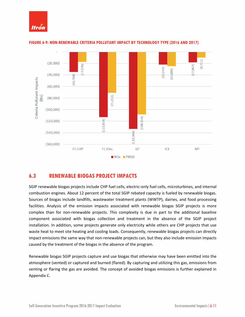
Self-Generation Incentive Program 2016-2017 Impact Evaluation Environmental Impacts|6-11
FIGURE 6-9: NON-RENEWABLE CRITERIA POLLUTANT IMPACT BY TECHNOLOGY TYPE (2016 AND 2017)
6.3 RENEWABLE BIOGAS PROJECT IMPACTS
SGIP renewable biogas projects include CHP fuel cells, electric-only fuel cells, microturbines, and internal combustion engines. About 12 percent of the total SGIP rebated capacity is fueled by renewable biogas. Sources of biogas include landfills, wastewater treatment plants (WWTP), dairies, and food processing facilities. Analysis of the emission impacts associated with renewable biogas SGIP projects is more complex than for non-renewable projects. This complexity is due in part to the additional baseline component associated with biogas collection and treatment in the absence of the SGIP project installation. In addition, some projects generate only electricity while others are CHP projects that use waste heat to meet site heating and cooling loads. Consequently, renewable biogas projects can directly impact emissions the same way that non-renewable projects can, but they also include emission impacts caused by the treatment of the biogas in the absence of the program.
Renewable biogas SGIP projects capture and use biogas that otherwise may have been emitted into the atmosphere (vented) or captured and burned (flared). By capturing and utilizing this gas, emissions from venting or flaring the gas are avoided. The concept of avoided biogas emissions is further explained in Appendix C.

Self-Generation Incentive Program 2016-2017 Impact Evaluation Environmental Impacts|6-12
6.3.1 Renewable Biogas Project Greenhouse Gas Impacts
When reporting emissions impacts from different types of greenhouse gases, total GHG emissions are reported in terms of metric tons of CO2 equivalent (CO2eq) so that direct comparisons can be made across technologies and energy sources. On a per mass unit basis, the global warming potential of CH4 is 21 times that of CO2. The biogas baseline estimates of vented emissions (CH4 emissions from renewable SGIP facilities) are converted to CO2eq by multiplying the metric tons of CH4 by 21. In this section, CO2eq emissions are reported if projects with a biogas venting baseline are included, otherwise; CO2 emissions are reported.
The annual GHG performance of renewable biogas SGIP projects are summarized below in Figure 6-10 by technology type and biogas baseline. CHP fuel cells, electric-only fuel cells, IC engines, and microturbines are all deployed in locations that would have otherwise flared biogas. Internal combustion engines were the only technology deployed at locations, such as dairies, which would have otherwise vented biogas.
FIGURE 6-10: RENEWABLE BIOGAS GREENHOUSE GAS IMPACT RATES BY TECHNOLOGY AND BIOGAS BASELINE TYPE (2016 AND 2017)
Figure 6-11 displays the same renewable biogas GHG impact rates as displayed in Figure 6-10, but further differentiates the fuel source by onsite biogas and directed biogas. As shown, directed biogas was only utilized at fuel cells, while all other, non-fuel cell technologies relied on onsite biogas. Renewable electric-only fuel cells relied solely on directed biogas.

Self-Generation Incentive Program 2016-2017 Impact Evaluation Environmental Impacts|6-13
FIGURE 6-11: RENEWABLE BIOGAS GREENHOUSE GAS IMPACT RATES BY TECHNOLOGY, BIOGAS SOURCE, AND BIOGAS BASELINE TYPE (2016 AND 2017)
All renewable biogas technologies reduced GHG emissions regardless of the biogas baseline type. Most technologies with flaring biogas achieved reductions between 0.16 and 0.49 metric tons of CO2 per MWh. Microturbines and electric-only fuel cells in 2017 were the exceptions. Internal combustion engines with vented biogas baselines achieved GHG reductions that were an over of magnitude greater, between 5.52 and 7.61 metric tons of CO2eq per MWh. The individual components contributing to renewable emissions impacts for each technology and biogas baseline are listed in Table 6-3 and Table 6-4 for 2016 and 2017 respectively.
TABLE 6-3: RENEWABLE GREENHOUSE GAS IMPACTS BY TECHNOLOGY TYPE (2016)
Technology Type
Metric Tons of CO2eq per MWh Annual Energy
Generation [MWh]
SGIP Emissions
(A)
Electric Power Plant Emissions
(B)
Heating Services
(C)
Biogas Treatment
(D)
Total Avoided Emissions
(E = B+C+D)
Emissions Impact
(F = A-E) FC - CHP (Flare) 0.47 0.43 - 0.39 0.83 (0.36) 64,258
FC - Elec. (Flare) 0.44 0.43 - 0.31 0.74 (0.30) 95,448
ICE (Flare) 0.77 0.44 0.05 0.77 1.25 (0.49) 123,251 ICE (Vent) 0.77 0.44 - 5.85 6.29 (5.52) 7,444
MT (Flare) 0.83 0.44 0.03 0.83 1.30 (0.47) 7,364

Self-Generation Incentive Program 2016-2017 Impact Evaluation Environmental Impacts|6-14
TABLE 6-4: RENEWABLE GREENHOUSE GAS IMPACTS BY TECHNOLOGY TYPE (2017)
Technology Type
Metric Tons of CO2eq per MWh Annual Energy
Generation [MWh]
SGIP Emissions
(A)
Electric Power Plant Emissions
(B)
Heating Services
(C)
Biogas Treatment
(D)
Total Avoided Emissions
(E = B+C+D)
Emissions Impact
(F = A-E) FC - CHP (Flare) 0.46 0.44 - 0.19 0.62 (0.16) 62,628
FC - Elec. (Flare) 0.42 0.43 - 0.12 0.55 (0.13) 142,607
ICE (Flare) 0.62 0.42 0.03 0.62 1.07 (0.45) 112,677
ICE (Vent) 0.62 0.43 - 4.71 5.15 (4.53) 12,500
MT (Flare) 0.81 0.42 - 0.81 1.23 (0.42) 5,911
The total CO2eq impact of renewable biogas projects is shown in Figure 6-12. Just over 40% of the total 2106 GHG impact for renewable CHP fuel cells came from directed biogas projects, while directed biogas in 2017 resulted in a small increase in GHG impacts due to biogas contracts expiring.2 All renewable electric-only fuel cell GHG impacts were from directed biogas projects.
FIGURE 6-12: RENEWABLE BIOGAS GREENHOUSE GAS IMPACT BY TECHNOLOGY AND BIOGAS BASELINE TYPE (2016 AND 2017)
2 For impact evaluation purposes we assume that all directed biogas projects consume biogas for five years from
their upfront payment date. After five years, directed biogas projects are assumed to consume 100% non-renewable natural gas.

Self-Generation Incentive Program 2016-2017 Impact Evaluation Environmental Impacts|6-15
6.3.2 Renewable Biogas Project Criteria Pollutant Impacts
The criteria pollutant emission impact rate of renewable biogas SGIP projects is summarized in Figure 6-13. All technologies with flaring biogas baseline reduce criteria pollutant impacts due to avoided emissions from the flare and from the grid baseline. Internal combustion engines with venting baselines do not significantly reduce criteria pollutants since the methane is only converted into criteria pollutants after the combustion process. In the baseline, the vented biogas remains as methane. CHP fuel cells with onsite biogas saw impact rates of 0.54 lb/MWh NOX and 0.17 lb/MWh PM10 while directed biogas projects had a higher impact rate of 0.08 lb/MWh and 0.06 lb/MWh for NOX and PM10, respectively.
FIGURE 6-13: RENEWABLE CRITERIA POLLUTANT IMPACT RATES BY TECHNOLOGY TYPE AND BIOGAS BASELINE (2016 AND 2017)
The total criteria pollutant impact for renewable biogas projects is shown in Figure 6-14. The total impact reduction attributable to directed biogas CHP fuel cell projects was almost 6,000 lbs of NOX and almost 4,000 lbs of PM10.

Self-Generation Incentive Program 2016-2017 Impact Evaluation Environmental Impacts|6-16
FIGURE 6-14: RENEWABLE CRITERIA POLLUTANT IMPACT BY TECHNOLOGY TYPE AND BIOGAS BASELINE (2016 AND 2017)
6.4 WIND AND PRESSURE REDUCTION TURBINE PROJECT IMPACTS
Wind and pressure reduction turbine projects (PRT) do not consume any type of fuel, and do not recover waste heat. Their emissions reduction rates (both for CO2 and criteria pollutants) are equal to the emissions rate of the grid, as described in Appendix C and Appendix D. The individual components contributing to wind and PRT GHG emissions are shown below in Table 6-5 and Table 6-6.
TABLE 6-5: WIND AND PRESSURE REDUCTION TURBINE GREENHOUSE GAS IMPACTS (2016)
Technology Type
Metric Tons of CO2 per MWh Annual Energy Impact [MWh]
SGIP Emissions
(A)
Electric Power Plant Emissions
(B)
Total Avoided Emissions
(C=B)
Emissions Impact
(D = A-C) PRT - 0.45 0.45 (0.45) 6,086 WD - 0.44 0.44 (0.44) 58,134

Self-Generation Incentive Program 2016-2017 Impact Evaluation Environmental Impacts|6-17
TABLE 6-6: WIND AND PRESSURE REDUCTION TURBINE GREENHOUSE GAS IMPACTS (2017)
Technology Type
Metric Tons of CO2 per MWh Annual Energy Impact [MWh]
SGIP Emissions
(A)
Electric Power Plant Emissions
(B)
Total Avoided Emissions
(C=B)
Emissions Impact
(D = A-C) PRT - 0.45 0.45 (0.45) 7,972 WD - 0.42 0.42 (0.42) 56,655
6.5 ADVANCED ENERGY STORAGE PROJECT IMPACTS
SGIP AES projects increase customer load when they charge, and they decrease load when they discharge. When load is increased, GHG emissions generally increase. Conversely, when load is reduced, GHG emissions are avoided. For AES projects to reduce GHG emissions, the GHG avoided during storage discharge must be greater than the GHG increase during storage charging. Since AES technologies inherently consume more energy during charging relative to energy discharged, the marginal emissions rate must be lower during charging hours relative to discharge hours. In other words, SGIP storage projects must charge during “cleaner” grid hours and discharge during “dirtier” grid hours to achieve GHG reductions. SGIP GHG impacts during 2016 and 2017 are summarized below in Figure 6-15 and Figure 6-16.
GHG impacts for all SGIP AES projects are positive during 2016 and 2017, reflecting increased emissions. The magnitude and the sign of GHG impacts is dependent on the timing of AES charging and discharging.
FIGURE 6-15: AVERAGE CO2 EMISSIONS PER SGIP REBATED CAPACITY (2016)

Self-Generation Incentive Program 2016-2017 Impact Evaluation Environmental Impacts|6-18
FIGURE 6-16: AVERAGE CO2 EMISSIONS PER SGIP REBATED CAPACITY (2017)
The evaluation team also estimated the impact that inefficiencies associated with parasitic losses have on the net GHG emissions for nonresidential projects (this analysis was conducted only in 2017). Figure 6-17 presents the influence these losses have on the overall GHG impacts for our sample of non-PBI nonresidential projects.3 Parasitic losses account for roughly 10% of the net GHG increase for non-PBI projects. While significant, it is notable that eliminating these parasitic losses is not sufficient to turn the fleet of non-PBI nonresidential projects into GHG reducers. The timing of charge/discharge relative to the grid marginal emissions rate remains the most important factor.
FIGURE 6-17: WATERFALL OF TOTAL CO2 IMPACTS FOR 2017 NON-PBI NONRESIDENTIAL PROJECTS (INCLUDING PARASITIC INFLUENCE)
3 The GHG increase in this figure represents the sample-level impact.

Self-Generation Incentive Program 2016-2017 Impact Evaluation Environmental Impacts|6-19
The criteria pollutant grid marginal emission shape is derived from similar inputs as the CO2 shape. Consequently, the results for SGIP AES criteria pollutant impacts are consistent with the CO2 impact findings discussed above. Both PBI and non-PBI AES projects increased PM10 and NOx emissions due to the timing of their charge/discharge and increased energy consumption due to losses. This analysis was only conducted in 2017. Results are summarized in Figure 6-18 and Figure 6-19.
FIGURE 6-18: AVERAGE PM10 EMISSIONS PER REBATED CAPACITY FOR ALL PROJECTS (2017)
FIGURE 6-19: NOX EMISSIONS PER REBATED CAPACITY FOR ALL PROJECTS (2017)
Total AES population GHG impacts during 2016 and 2017 are summarized in Table 6-7. Greenhouse gas impacts for both PBI and non-PBI are positive, reflecting increased emissions. The magnitude and the sign of greenhouse gas impacts is very dependent on the timing of AES charging and discharging. While the

Self-Generation Incentive Program 2016-2017 Impact Evaluation Environmental Impacts|6-20
timing of AES charging and discharging produced valuable reductions in summer-time customer peak demand, one consequence of that timing was an increase in greenhouse gas emissions. We observe similar results for NOx and PM10 impacts in 2017, as shown in Table 6-8 and Table 6-9.
TABLE 6-7: AES GREENHOUSE GAS IMPACTS
Year Customer Sector N Population Impact (MT C02)
Relative Precision
2016 Nonresidential PBI 83 441 6% Nonresidential Non-PBI 246 285 5% Total 329 726 4%
2017
Nonresidential PBI 143 974 4% Nonresidential Non-PBI 278 462 9% Residential 407 116 18% Total 828 1,552 4%
TABLE 6-8: AES NOX IMPACTS
Year Customer Sector N Population Impact (lbs NOx) Relative Precision
2017
Nonresidential PBI 143 6 279% Nonresidential Non-PBI 278 108 9% Residential 407 30 20% Total 828 144 15%
TABLE 6-9: AES PM10 IMPACTS
Year Customer Sector N Population Impact (lbs PM10) Relative Precision
2017
Nonresidential PBI 143 157 3% Nonresidential Non-PBI 278 61 9% Residential 407 15 18% Total 828 234 3%

Self-Generation Incentive Program 2016-2017 Impact Evaluation Appendix A: Program Statistics|A-1
APPENDIX A PROGRAM STATISTICS This appendix provides detailed Self-Generation Incentive Program (SGIP) statistics beyond the tables and figures included in Section 2.
A.1 PROGRAM STATISTICS
At the end of 2017, the SGIP had paid incentives to 1,768 projects representing 568 MW of rebated capacity. Table A-1 shows this counts and rebated capacities of all completed projects by program administrator (PA). PG&E made up 43% of all completed rebated capacity installed through the SGIP, followed by SCE at 23%, SCG and 22%, and CSE at 12%.
TABLE A-1: COMPLETED PROJECT COUNT AND REBATED CAPACITY BY PROGRAM ADMINISTRATOR
Program Administrator Project Count Rebated Capacity [MW] Percent of Rebated Capacity
CSE 312 70 12% PG&E 753 243 43% SCE 507 129 23% SCG 196 125 22%
Total 1,768 568 100%
The variety of technology types receiving incentives are shown below in Table A-2.
TABLE A-2: COMPLETED PROJECT COUNT AND REBATED CAPACITY BY TECHNOLOGY TYPE
Technology Type Project Count Average Capacity [kW]
Total Rebated Capacity [MW]
Percent of Rebated Capacity
Advanced Energy Storage 830 86 72 13% Fuel Cell - CHP 126 340 43 8% Fuel Cell - Electric Only 319 410 131 23% Gas Turbine 13 4,204 55 10% Internal Combustion Engine 290 677 196 35%
Microturbine 157 237 37 7% Pressure Reduction Turbine 6 510 3 1%
Wind 26 1,207 31 6% Waste Heat to Power 1 125 0.1 0.0% Total 1,768 321 568 100%

Self-Generation Incentive Program 2016-2017 Impact Evaluation Appendix A: Program Statistics|A-2
One focus in this evaluation has been to separate out the differences between those projects taking a performance-based incentive (PBI) payment and those without. The breakout of project counts and rebated capacities of completed projects by technology and incentive payment mechanism are shown below in Table A-3.
TABLE A-3: COMPLETED PROJECT COUNT AND REBATED CAPACITY BY PBI VS. NON-PBI
Technology Type
PBI Non-PBI
Rebated Capacity [MW] Count of Projects Rebated Capacity
[MW] Count of Projects
AES 62 145 10 685 FC-CHP 9 10 34 116 FC-Elec. 90 229 41 90 GT 25 4 30 9
ICE 40 34 156 256 MT 11 14 26 143 PRT 3 6 0 0 WD 18 9 14 17 WHP 0.1 1 0 0 Total 258 452 311 1,316
SGIP projects are fueled by a variety of renewable and non-renewable energy sources. The majority of SGIP projects are powered by non-renewable fuels such as natural gas. On-site biogas projects typically use biogas derived from landfills or anaerobic digestion processes that convert biological matter to a renewable fuel source. Anaerobic digesters are used at dairies, wastewater treatment plants, or food processing facilities to convert wastes from these facilities to biogas. Directed biogas projects purchase biogas fuel that is produced at a location other than the project site. The ‘Other’ energy source group includes advanced energy storage, wind turbine, waste heat to power, and pressure reduction turbine projects. These are displayed in Table A-4.

Self-Generation Incentive Program 2016-2017 Impact Evaluation Appendix A: Program Statistics|A-3
TABLE A-4: COMPLETED PROJECT COUNT AND REBATED CAPACITY BY TECHNOLOGY TYPE AND ENERGY SOURCE
Technology Type Energy Source Total Rebated Capacity [MW] Count of Projects Percent of Rebated
Capacity
AES Other 72 830 13%
FC-CHP
Non-Renewable 22 104 4% On-site Biogas 14 16 2%
Directed Biogas 7 6 1%
FC-Elec. Non-Renewable 102 260 18% Directed Biogas 29 59 5%
GT Non-Renewable 55 13 10%
ICE Non-Renewable 159 243 28% On-site Biogas 37 47 7%
MT Non-Renewable 28 126 5% On-site Biogas 9 31 2%
PRT Other 3 6 1% WD Other 31 26 6%
WHP Other 0 1 0% Total 568 1,768 100%
Combined heat and power (CHP) projects can recover useful heat to serve heating loads such as process hot water or cooling loads by use of an absorption chiller. The useful heat end use has important implications for natural gas distribution impacts and consequently greenhouse gas emissions impacts. Table A-5 summarizes the useful heat end uses observed in the SGIP.
TABLE A-5: PROJECT COUNTS AND REBATED CAPACITIES FOR PROJECTS WITH USEFUL HEAT RECOVERY BY USEFUL HEAT END USE
Useful Heat End Use Project Count Rebated Capacity [MW]
Percent of Rebated Capacity
Cooling Only 47 46.5 15% Heating Only 412 188.6 60% Heating and Cooling 95 80.1 25% Total 554 315.2 100%
* Technologies excluded from total capacity include advanced energy storage, pressure reduction turbines, wind turbines, and other generation technologies exempt from heat recovery requirements.
By the end of 2017, the SGIP paid or reserved $845 million in incentives. Eligible costs reported by applicants surpassed $3 billion. Table A-6 shows the breakdown of incentives paid by the SGIP and costs reported by applicants for each technology type. The leverage ratio, calculated as the ratio of SGIP participant investment to SGIP incentives, is one financial measure of the SGIP’s effectiveness in accelerating development of markets for distributed energy resources.

Self-Generation Incentive Program 2016-2017 Impact Evaluation Appendix A: Program Statistics|A-4
TABLE A-6: INCENTIVES PAID, REPORTED COSTS, AND LEVERAGE RATIO BY TECHNOLOGY TYPE
Technology Type Rebated Capacity [MW]
SGIP Incentive [Nominal $MM]
Eligible Costs [Nominal $MM] Leverage Ratio
AES 72 $126 $245 0.93 FC-CHP 43 $125 $326 1.61 FC-Elec. 131 $380 $1,506 2.96 GT 55 $10 $148 13.18
ICE 196 $136 $522 2.85 MT 37 $32 $139 3.36 PRT 3 $3 $13 3.94 WD 31 $33 $119 2.62 Total 568 $845 $3,018 2.57
SGIP projects are electrically interconnected to load serving entities that are either investor owned (IOU) or municipal utilities. Table A-7 shows each PA’s rebated capacity by electric utility type and technology type. Almost 92% of rebated capacity was interconnected to investor owned electric utilities.
TABLE A-7: REBATED CAPACITIES OF SGIP PROJECTS BY ELECTRIC UTILITY TYPE, PROGRAM ADMINISTRATOR, AND TECHNOLOGY TYPE
Program Administrator
Electric Utility Type AES FC-
CHP FC-
Elec. GT ICE MT PRT WD WHP All Proj.
CSE IOU 16 10 11 18 11 2 1 1 - 70
Municipal - - - - - - - - - -
PG&E IOU 29 13 62 15 83 15 1 15 0.1 235
Municipal 0 - 2 - 6 - - - - 9
SCE IOU 26 7 33 - 39 9 0 15 - 129
Municipal - - - - - - - - - -
SCG IOU 1 6 1 17 54 7 - - - 86
Municipal 0 6 22 4 3 3 - - - 39 Total 72 43 131 55 196 37 3 31 0.1 568
A.2 PROGRAM STATISTICS TRENDS
The date a project is issued its upfront payment is used as a proxy for the date it enters normal operations and begins to accrue impacts. Table A-8 and Table A-9 display the project counts and capacities by technology type and upfront payment year. Table A-8 shows the annual counts and capacities while Table A-9 shows cumulative counts and capacities.

Self-Generation Incentive Program 2016-2017 Impact Evaluation Appendix A: Program Statistics|A-5
TABLE A-8: PROJECT COUNTS AND REBATED CAPACITY BY TECHNOLOGY TYPE AND UPFRONT PAYMENT YEAR
Upfront Payment Year Metric AES FC-
CHP FC-
Elec. GT ICE MT PRT WD WHP All Proj.
2001
Count 0 0 0 0 2 1 0 0 0 3 Capacity [MW] - - - - 0.6 0.1 - - - 0.6
2002
Count 0 1 0 0 19 14 0 0 0 34 Capacity [MW] - 0.2 - - 11.9 1.9 - - - 14.0
2003
Count 0 0 0 0 53 27 0 0 0 80 Capacity [MW] - - - - 41.3 3.9 - - - 45.2
2004
Count 0 1 0 1 51 22 0 1 0 76 Capacity [MW] - 0.6 - 1.4 29.4 2.9 - 1.0 - 35.2
2005 Count 0 4 0 3 48 26 0 1 0 82
Capacity [MW] - 2.8 - 7.1 24.6 5.1 - 0.7 - 40.3
2006 Count 0 7 0 1 26 25 0 0 0 59
Capacity [MW] - 4.0 - 4.5 15.8 4.4 - - - 28.6
2007 Count 0 4 0 1 25 12 0 0 0 42
Capacity [MW] - 2.4 - 4.6 15.6 1.8 - - - 24.4
2008 Count 0 3 1 2 8 8 0 0 0 22
Capacity [MW] - 2.1 0.4 8.1 7.0 2.1 - - - 19.6
2009 Count 0 3 1 0 8 3 0 3 0 18
Capacity [MW] - 2.1 0.3 - 1.9 1.7 - 1.3 - 7.3
2010 Count 0 26 14 0 12 2 0 3 0 57
Capacity [MW] - 1.4 6.7 - 6.4 0.3 - 1.8 - 16.6
2011 Count 1 52 43 1 4 1 0 4 0 106
Capacity [MW] 1.0 5.0 17.2 4.4 2.0 0.8 - 4.6 - 34.9
2012 Count 2 10 41 0 0 3 0 7 0 63
Capacity [MW] 0.9 11.3 22.8 - - 0.9 - 14.0 - 49.9
2013 Count 13 4 35 1 2 2 1 2 0 60
Capacity [MW] 1.1 2.8 16.1 4.6 5.2 1.3 0.7 1.5 - 33.5
2014 Count 47 3 16 1 7 4 0 1 0 79
Capacity [MW] 1.5 0.0 10.5 11.3 6.1 4.4 - 1.3 - 35.0
2015 Count 281 4 69 1 14 0 1 3 0 373
Capacity [MW] 18.5 3.8 26.2 4.2 14.3 - 1.2 4.4 - 72.5
2016 Count 373 2 56 1 4 2 3 0 0 441
Capacity [MW] 29.6 2.3 15.2 4.4 4.7 1.8 0.6 - - 58.5
2017 Count 113 2 43 0 7 5 1 1 1 173
Capacity [MW] 19.1 2.2 15.5 - 9.7 3.8 0.5 1.0 0.1 51.9
Total Count 830 126 319 13 290 157 6 26 1 1,768
Capacity [MW] 71.6 42.9 130.9 54.6 196.4 37.1 3.1 31.4 0.1 568.2

Self-Generation Incentive Program 2016-2017 Impact Evaluation Appendix A: Program Statistics|A-6
TABLE A-9: CUMULATIVE PROJECT COUNTS AND REBATED CAPACITY BY TECHNOLOGY TYPE AND UPFRONT PAYMENT YEAR
Upfront Payment Year Metric AES FC-
CHP FC-
Elec. GT ICE MT PRT WD WHP All Proj.
2001
Count 0 0 0 0 2 1 0 0 0 3 Capacity [MW] 0.0 0.0 0.0 0.0 0.6 0.1 0.0 0.0 0.0 0.6
2002
Count 0 1 0 0 21 15 0 0 0 37 Capacity [MW] 0.0 0.2 0.0 0.0 12.4 2.0 0.0 0.0 0.0 14.7
2003
Count 0 1 0 0 74 42 0 0 0 117 Capacity [MW] 0.0 0.2 0.0 0.0 53.8 5.9 0.0 0.0 0.0 59.9
2004
Count 0 2 0 1 125 64 0 1 0 193 Capacity [MW] 0.0 0.8 0.0 1.4 83.2 8.8 0.0 1.0 0.0 95.1
2005 Count 0 6 0 4 173 90 0 2 0 275
Capacity [MW] 0.0 3.6 0.0 8.5 107.8 13.9 0.0 1.6 0.0 135.5
2006 Count 0 13 0 5 199 115 0 2 0 334
Capacity [MW] 0.0 7.5 0.0 13.0 123.6 18.3 0.0 1.6 0.0 164.1
2007 Count 0 17 0 6 224 127 0 2 0 376
Capacity [MW] 0.0 9.9 0.0 17.6 139.3 20.1 0.0 1.6 0.0 188.5
2008 Count 0 20 1 8 232 135 0 2 0 398
Capacity [MW] 0.0 11.9 0.4 25.7 146.3 22.1 0.0 1.6 0.0 208.1
2009 Count 0 23 2 8 240 138 0 5 0 416
Capacity [MW] 0.0 14.0 0.7 25.7 148.1 23.8 0.0 2.9 0.0 215.3
2010 Count 0 49 16 8 252 140 0 8 0 473
Capacity [MW] 0.0 15.4 7.4 25.7 154.5 24.1 0.0 4.7 0.0 231.9
2011 Count 1 101 59 9 256 141 0 12 0 579
Capacity [MW] 1.0 20.5 24.6 30.1 156.5 24.9 0.0 9.3 0.0 266.8
2012 Count 3 111 100 9 256 144 0 19 0 642
Capacity [MW] 1.9 31.7 47.4 30.1 156.5 25.8 0.0 23.2 0.0 316.7
2013 Count 16 115 135 10 258 146 1 21 0 702
Capacity [MW] 3.0 34.6 63.6 34.7 161.7 27.1 0.7 24.7 0.0 350.1
2014 Count 63 118 151 11 265 150 1 22 0 781
Capacity [MW] 4.5 34.6 74.1 46.1 167.7 31.5 0.7 26.0 0.0 385.2
2015 Count 344 122 220 12 279 150 2 25 0 1154
Capacity [MW] 22.9 38.4 100.2 50.3 182.0 31.5 1.9 30.4 0.0 457.7
2016 Count 717 124 276 13 283 152 5 25 0 1595
Capacity [MW] 52.5 40.7 115.4 54.6 186.7 33.3 2.5 30.4 0.0 516.1
2017 Count 830 126 319 13 290 157 6 26 1 1768
Capacity [MW] 71.6 42.9 130.9 54.6 196.4 37.1 3.1 31.4 0.1 568.2
A project’s program year is used to determine what program rules and policies are applicable to it. Table A-10 and Table A-11 list project counts and rebated capacities by program year and technology type for projects paid on or before December 31st, 2017. Table A-10 shows the annual counts and capacities while Table A-11 shows the cumulative counts and capacities.

Self-Generation Incentive Program 2016-2017 Impact Evaluation Appendix A: Program Statistics|A-7
TABLE A-10: PROJECT COUNTS AND REBATED CAPACITY BY TECHNOLOGY TYPE AND PROGRAM YEAR
Program Year Metric AES FC-CHP
FC-Elec. GT ICE MT PRT WD WHP All
Proj.
PY01 Count 0 1 0 0 27 21 0 0 0 49
Capacity [MW] - 0.2 - - 14.7 2.8 - - - 17.7
PY02 Count 0 1 0 1 54 17 0 0 0 73
Capacity [MW] - 0.6 - 1.4 36.5 2.9 - - - 41.4
PY03 Count 0 2 0 1 54 40 0 2 0 99
Capacity [MW] - 0.8 - 1.2 37.5 5.0 - 1.6 - 46.1
PY04 Count 0 3 0 1 49 30 0 0 0 83
Capacity [MW] - 2.3 - 1.4 24.6 5.7 - - - 33.9
PY05 Count 0 6 0 2 31 14 0 0 0 53
Capacity [MW] - 3.7 - 9.0 22.4 3.1 - - - 38.2
PY06 Count 0 7 0 3 17 13 0 0 0 40
Capacity [MW] - 5.1 - 12.7 11.2 4.1 - - - 33.1
PY07 Count 0 2 1 1 24 7 0 2 0 37
Capacity [MW] - 0.8 0.4 4.4 9.6 2.1 - 1.2 - 18.4
PY08 Count 0 6 0 0 0 0 0 1 0 7
Capacity [MW] - 0.6 - - - - - 0.2 - 0.9
PY09 Count 1 18 8 0 0 0 0 3 0 30
Capacity [MW] 1.0 7.3 2.7 - - - - 1.6 - 12.6
PY10 Count 1 64 80 0 0 0 0 7 0 152
Capacity [MW] 0.6 12.4 37.6 - - - - 9.1 - 59.7
PY11 Count 26 3 20 0 1 1 0 5 0 56
Capacity [MW] 2.8 0.8 12.6 - 0.7 0.8 - 11.0 - 28.6
PY12 Count 218 7 39 3 15 8 2 3 0 295
Capacity [MW] 9.7 1.4 17.4 20.1 23.3 5.2 1.9 4.4 - 83.5
PY13 Count 114 2 32 1 3 2 0 2 1 157
Capacity [MW] 9.7 2.0 19.2 4.4 1.6 1.8 - 1.3 0.1 40.0
PY14 Count 380 2 85 0 8 2 2 1 0 480
Capacity [MW] 30.1 2.8 24.3 - 3.3 1.9 0.5 1.0 - 63.8
PY15 Count 82 2 50 0 5 1 2 0 0 142
Capacity [MW] 17.0 2.2 14.7 - 9.5 0.2 0.6 - - 44.3
PY16 Count 8 0 4 0 2 1 0 0 0 15
Capacity [MW] 0.8 - 1.9 - 1.6 1.6 - - - 5.9
PY17 Count 0 0 0 0 0 0 0 0 0 0
Capacity [MW] - - - - - - - - - 0.0
Total Count 830 126 319 13 290 157 6 26 1 1,768
Capacity [MW] 71.6 42.9 130.9 54.6 196.4 37.1 3.1 31.4 0.1 568.2

Self-Generation Incentive Program 2016-2017 Impact Evaluation Appendix A: Program Statistics|A-8
TABLE A-11: CUMULATIVE PROJECT COUNTS AND REBATED CAPACITY BY TECHNOLOGY TYPE AND PROGRAM YEAR
Program Year Metric AES FC-CHP
FC-Elec. GT ICE MT PRT WD WHP All
Proj.
PY01 Count 0 1 0 0 27 21 0 0 0 49
Capacity [MW] 0.0 0.2 0.0 0.0 14.7 2.8 0.0 0.0 0.0 17.7
PY02 Count 0 2 0 1 81 38 0 0 0 122
Capacity [MW] 0.0 0.8 0.0 1.4 51.3 5.7 0.0 0.0 0.0 59.1
PY03 Count 0 4 0 2 135 78 0 2 0 221
Capacity [MW] 0.0 1.6 0.0 2.6 88.8 10.7 0.0 1.6 0.0 105.2
PY04 Count 0 7 0 3 184 108 0 2 0 304
Capacity [MW] 0.0 3.8 0.0 4.0 113.3 16.3 0.0 1.6 0.0 139.1
PY05 Count 0 13 0 5 215 122 0 2 0 357
Capacity [MW] 0.0 7.5 0.0 13.0 135.7 19.5 0.0 1.6 0.0 177.3
PY06 Count 0 20 0 8 232 135 0 2 0 397
Capacity [MW] 0.0 12.6 0.0 25.7 146.9 23.6 0.0 1.6 0.0 210.5
PY07 Count 0 22 1 9 256 142 0 4 0 434
Capacity [MW] 0.0 13.4 0.4 30.1 156.5 25.6 0.0 2.9 0.0 228.9
PY08 Count 0 28 1 9 256 142 0 5 0 441
Capacity [MW] 0.0 14.0 0.4 30.1 156.5 25.6 0.0 3.1 0.0 229.8
PY09 Count 1 46 9 9 256 142 0 8 0 471
Capacity [MW] 1.0 21.3 3.1 30.1 156.5 25.6 0.0 4.7 0.0 242.3
PY10 Count 2 110 89 9 256 142 0 15 0 623
Capacity [MW] 1.6 33.7 40.7 30.1 156.5 25.6 0.0 13.8 0.0 302.0
PY11 Count 28 113 109 9 257 143 0 20 0 679
Capacity [MW] 4.4 34.5 53.3 30.1 157.1 26.4 0.0 24.7 0.0 330.7
PY12 Count 246 120 148 12 272 151 2 23 0 974
Capacity [MW] 14.1 35.9 70.7 50.3 180.5 31.6 1.9 29.1 0.0 414.1
PY13 Count 360 122 180 13 275 153 2 25 1 1,131
Capacity [MW] 23.8 37.9 90.0 54.6 182.0 33.4 1.9 30.4 0.1 454.2
PY14 Count 740 124 265 13 283 155 4 26 1 1,611
Capacity [MW] 53.8 40.7 114.2 54.6 185.3 35.4 2.4 31.4 0.1 517.9
PY15 Count 822 126 315 13 288 156 6 26 1 1,753
Capacity [MW] 70.8 42.9 129.0 54.6 194.8 35.5 3.1 31.4 0.1 562.2
PY16 Count 830 126 319 13 290 157 6 26 1 1,768
Capacity [MW] 71.6 42.9 130.9 54.6 196.4 37.1 3.1 31.4 0.1 568.2
PY17 Count 830 126 319 13 290 157 6 26 1 1,768
Capacity [MW] 71.6 42.9 130.9 54.6 196.4 37.1 3.1 31.4 0.1 568.2

Self-Generation Incentive Program 2016-2017 Impact Evaluation Appendix A: Program Statistics|A-9
Table A-12 lists the total incentives, eligible costs, and leverage ratio by technology type and program year.
TABLE A-12: PROJECT INCENTIVES, COSTS, AND LEVERAGE RATIO BY TECHNOLOGY TYPE AND PROGRAM YEAR
Program Year Metric AES FC-CHP FC-Elec. GT ICE MT PRT WD WHP All Proj.
PY01
Incentive $- $0.50 $- $- $9.04 $2.22 $- $- $- $11.76 Cost $- $3.60 $- $- $30.71 $8.14 $- $- $- $42.45
Leverage - 0.86 - - 0.71 0.73 - - - 0.72
PY02
Incentive $- $1.50 $- $0.81 $20.67 $2.33 $- $- $- $25.31 Cost $- $4.26 $- $3.73 $81.12 $8.41 $- $- $- $97.53
Leverage - 0.65 - 0.78 0.75 0.72 - - - 0.74
PY03
Incentive $- $3.38 $- $1.00 $21.54 $4.78 $- $2.63 $- $33.33 Cost $- $7.28 $- $4.69 $81.33 $17.41 $- $5.38 $- $116.09
Leverage - 0.54 - 0.79 0.74 0.73 - 0.51 - 0.71
PY04
Incentive $- $5.58 $- $1.00 $16.86 $5.07 $- $- $- $28.51 Cost $- $16.97 $- $7.18 $61.53 $17.50 $- $- $- $103.19
Leverage - 0.67 - 0.86 0.73 0.71 - - - 0.72
PY05
Incentive $- $7.89 $- $1.05 $12.13 $2.85 $- $- $- $23.92 Cost $- $22.46 $- $13.30 $53.58 $11.62 $- $- $- $100.96
Leverage - 0.65 - 0.92 0.77 0.75 - - - 0.76
PY06
Incentive $- $19.46 $- $1.80 $6.96 $3.28 $- $- $- $31.50 Cost $- $37.43 $- $29.57 $29.78 $14.08 $- $- $- $110.86
Leverage - 0.48 - 0.94 0.77 0.77 - - - 0.72
PY07 Incentive $- $2.00 $1.00 $0.60 $6.61 $2.02 $- $1.84 $- $14.07
Cost $- $4.47 $3.85 $1.38 $34.30 $7.88 $- $6.35 $- $58.24 Leverage - 0.55 0.74 0.56 0.81 0.74 - 0.71 - 0.76
PY08 Incentive $- $2.78 $- $- $- $- $- $0.26 $- $3.03
Cost $- $5.98 $- $- $- $- $- $0.35 $- $6.33 Leverage - 0.54 - - - - - 0.25 - 0.52

Self-Generation Incentive Program 2016-2017 Impact Evaluation Appendix A: Program Statistics|A-10
Program Year Metric AES FC-CHP FC-Elec. GT ICE MT PRT WD WHP All Proj.
PY09
Incentive $2.00 $23.54 $11.50 $- $- $- $- $2.41 $- $39.45 Cost $6.49 $62.49 $30.51 $- $- $- $- $5.14 $- $104.62
Leverage 0.69 0.62 0.62 - - - - 0.53 - 0.62
PY10
Incentive $1.20 $40.02 $159.79 $- $- $- $- $9.75 $- $210.77 Cost $5.17 $90.73 $390.09 $- $- $- $- $33.46 $- $519.45
Leverage 0.77 0.56 0.59 - - - - 0.71 - 0.59
PY11
Incentive $3.93 $1.81 $34.71 $- $1.63 $0.44 $- $9.47 $- $51.98 Cost $6.77 $7.18 $158.96 $- $2.55 $2.83 $- $40.36 $- $218.65
Leverage 0.42 0.75 0.78 - 0.36 0.85 - 0.77 - 0.76
PY12
Incentive $19.84 $3.09 $46.58 $3.17 $29.35 $4.80 $1.31 $3.75 $- $111.89 Cost $34.86 $14.18 $204.74 $67.38 $78.90 $29.79 $4.70 $17.07 $- $451.62
Leverage 0.43 0.78 0.77 0.95 0.63 0.84 0.72 0.78 - 0.75
PY13
Incentive $17.61 $3.86 $46.14 $1.01 $0.72 $2.48 $- $1.44 $0.18 $73.43 Cost $31.63 $17.12 $238.75 $20.73 $6.80 $7.79 $- $5.57 $0.48 $328.87
Leverage 0.44 0.77 0.81 0.95 0.89 0.68 - 0.74 0.63 $5.92
PY14
Incentive $53.09 $6.34 $47.90 $- $4.76 $0.86 $0.55 $1.36 $- $114.86 Cost $103.51 $18.80 $279.94 $- $18.46 $6.19 $3.46 $5.60 $- $435.96
Leverage 0.49 0.66 0.83 - 0.74 0.86 0.84 0.76 - 0.74
PY15
Incentive $27.76 $3.30 $29.06 $- $2.63 $0.10 $0.68 $- $- $63.53 Cost $54.44 $13.12 $177.26 $- $29.78 $1.24 $4.42 $- $- $280.25
Leverage 0.49 0.75 0.84 - 0.91 0.92 0.85 - - 0.77
PY16
Incentive $1.07 $- $3.20 $- $2.77 $0.65 $- $- $- $7.68 Cost $1.80 $- $21.75 $- $13.62 $5.95 $- $- $- $43.12
Leverage 0.41 - 0.85 - 0.80 0.89 - - - 0.82
PY17 Incentive $- $- $- $- $- $- $- $- $- $-
Cost $- $- $- $- $- $- $- $- $- $- Leverage - - - - - - - - - -

Self-Generation Incentive Program 2016-2017 Impact Evaluation Appendix A: Program Statistics|A-11
Program Year Metric AES FC-CHP FC-Elec. GT ICE MT PRT WD WHP All Proj.
Total
Incentive $126.49 $125.05 $379.88 $10.44 $135.66 $31.88 $2.55 $32.90 $0.18 $845.02 Cost $244.66 $326.07 $1,505.85 $147.97 $522.47 $138.83 $12.58 $119.27 $0.48 $3,018.19
Leverage 0.48 0.62 0.75 0.93 0.74 0.77 0.80 0.72 0.63 $6.44

Self-Generation Incentive Program 2016-2017 Impact Evaluation Appendix B: Energy Impacts Estimation |B-1
APPENDIX B ENERGY IMPACTS ESTIMATION METHODOLOGY AND RESULTS
This appendix provides additional detail about the metered data and the ratio estimation methodology used to quantify the energy impacts of the Self-Generation Incentive Program (SGIP) in this evaluation report. This appendix also includes generation project energy and peak demand impacts detail not shown in Section 4. The focus of this section is estimation of impacts from generation projects, however we also discuss the ratio estimation process for energy storage projects. The following key topics are discussed in this appendix:
Estimation Methodology (Emphasis on Generation Projects)
─ Data Processing and Validation
─ Operational Status Research (OSR)
─ Ratio Estimation
Energy Impacts
Coincident Demand Impacts
B.1 ESTIMATION METHODOLOGY
Estimation of SGIP impacts relies on large datasets of metered electrical, fuel consumption and heat recovery. We use these data to estimate electrical generation, fuel consumption and heat recovery where we have no metered data that passes quality control validation. We multiply sums of metered impacts taken for a particular type of system over a particular period by of time by the ratio of sums of capacities without valid data to those with valid metered data. The impact estimate then is the sum of the metered and the estimated impact.
B.1.1 Data Processing and Validation
Electrical Net Generation Output (ENGO) Data
Metered electric NGO data provide information on the amount of electricity generated by SGIP projects net of ancillary loads such as pumps and compressors. These data are typically kWh recorded at 15-minute intervals but sometimes are at hourly or longer intervals or are average kW over the interval.
Electric NGO data are collected from a variety of sources, including meters installed by Itron and its subcontractors under the direction of the PAs, and meters installed by project hosts, applicants, electric utilities, and third parties. Because many different meters are in use among the many different providers,

Self-Generation Incentive Program 2016-2017 Impact Evaluation Appendix B: Energy Impacts Estimation |B-2
these electric NGO data arrive in a wide variety of data formats. Some formats require extensive processing to be associated with the correct project and put into a format common to all projects.
During processing to the common format, all electric NGO data pass through a rigorous quality control review. Only data that pass the review are accepted for use in this evaluation. Key factors in the review are system capacity, unit count, and technology. Some technologies can generate farther above nameplate capacity for longer periods than other technologies. Some technologies can generate at lower capacity factor for longer periods than other technologies. In addition, some fuel cells may consume substantial electricity during standby.
Fuel Consumption Data
Fuel consumption data are used in this impacts evaluation to determine system efficiencies and to estimate greenhouse gas (GHG) emission impacts. To date, fuel consumption data collection activities have focused exclusively on consumption of natural gas by SGIP projects. In the future, it may also be necessary to monitor consumption of gaseous renewable fuel (i.e., biogas) to more accurately assess the impacts of SGIP projects using blends of renewable and non-renewable fuels.
Fuel consumption data used in this impacts evaluation are obtained mostly in units of standard cubic feet or therms from natural gas metering systems installed on SGIP projects by natural gas distribution companies, SGIP participants, or by third parties. Itron reviews fuel consumption data and documents their bases prior to processing the data into a common data format and unit of MBtu LHV.
During processing of fuel consumption data, they are merged with electric NGO data for quality control reviews. The fuel data are examined for reasonableness of electrical conversion efficiency for the technology over the course of multiple hours or days. In cases where validity checks fail, data providers are contacted to further refine the basis of data, otherwise data are ignored as unrepresentative. In some cases, it is determined the data are for a host customer’s entire facility rather than from metering dedicated to the SGIP project.
Some fuel consumption data arrive already merged with NGO data but most fuel consumption data arrive in various formats and intervals much greater than one hour (e.g., in daily or monthly intervals). These longer interval data enable calculation of monthly and annual efficiencies but are not used to estimate performance for shorter intervals.
Useful Heat Recovery Data
Useful heat recovery is the thermal energy captured by heat recovery equipment and used to satisfy heating and/or cooling loads at the SGIP project site. Useful heat recovery data are used to assess overall

Self-Generation Incentive Program 2016-2017 Impact Evaluation Appendix B: Energy Impacts Estimation |B-3
efficiencies of SGIP projects and to estimate avoided baseline natural gas use. This avoided use is used in calculation of GHG emission impact estimates where it reduces net emissions.
Heat recovery data are collected from metering systems installed by Itron as well as metering systems installed by applicants, hosts, and third parties. Because many different meters are in use among the many different providers, these heat data arrive in a wide variety of data formats. Some formats require extensive processing to be associated with the correct project and put into a format common to all projects. Heat data may arrive in units of Btu or as flow with associated high and low temperatures. In the latter case, heat exchanger and fluid properties are identified in calculation of useful recovered MBtu.
Over the course of the SGIP, the approach for collecting useful heat recovery data has changed. Useful heat recovery data collection historically has involved installation of invasive monitoring equipment (i.e., insertion-type flow meters). Many third parties had this type of equipment installed at the time the SGIP project was commissioned, either as part of their contractual agreement with a third-party vendor or as part of an internal process/energy monitoring plan. In numerous cases, Itron obtains useful heat recovery data metered by others in an effort to minimize both the cost and disruption of installing useful heat recovery monitoring equipment. The majority of useful heat recovery data for years 2003 and 2004 were obtained in this manner.
Itron began installing useful heat recovery metering in the summer of 2003 for SGIP projects that were included in the sample design but for which data were not available. As the useful heat recovery data collection effort grew, it became clear that we could no longer rely on data from third party or host customer metering. In numerous instances, agreements and plans concerning these data did not yield valid data for analysis. Uninterrupted collection and validation of useful heat recovery data was labor-intensive and required examination of the data by more expert staff, thereby increasing costs. In addition, reliance on useful heat recovery data collected by SGIP host customers and third parties created evaluation schedule impacts and other risks that more than outweighed the benefits of not having to install new metering.
In mid-2006, Itron responded to the useful heat recovery data issues by changing the approach to collection of useful heat recovery data. We continued to collect useful heat recovery data from program participants in those instances where valid data could be obtained easily and reliably. For all other projects selected for metered data collection, we installed useful heat recovery metering systems ourselves. These systems utilized non-invasive components such as ultrasonic flow meters, clamp-on temperature sensors, and wireless, cellular-based communications to reduce the time and disruption of the installations and to increase data communication reliability. The increase in equipment costs was offset by the decrease in installation time and a decrease in maintenance problems.

Self-Generation Incentive Program 2016-2017 Impact Evaluation Appendix B: Energy Impacts Estimation |B-4
Operational Status Research
Using a short phone survey, we collected categorical operating status data on systems for which no metered data are available and that are not already known to be permanently retired. Completed surveys allow classification of system-months as offline or online. For offline system-months, we estimated impacts using a zero-ratio estimator. For online system months, we estimated impacts using a ratio estimator developed from similar systems whose metered data indicate they were online that same month. Some surveys identify systems as being permanently retired or decommissioned. We identify a best estimate of retirement date in the survey and estimate impacts from that date forward using a zero-ratio estimator.
Operational status research is conducted only with contacts familiar with the operational status of the unmetered system. The operating status survey identifies most recently known system contacts that may include system, hosts, applicants, or former data providers. Contact information from PA system lists, inspection reports, or site visit summaries are used. When these contacts are out of date, contact information may be sought from internet sources.
Ratio Estimation
Non-AES Project Approach
An overview of the ratio estimation methodology was included in Section 3. The strata included in the ratio analysis for electricity generation values were presented in Table 3-1, and are also listed below:
1. Technology type 2. Operational status 3. Program incentive structure (pre-SB 412 and post-SB 412) 4. Warranty status (under corresponding handbook) 5. Fuel type 6. Capacity size category 7. PA
The ratio estimation methodology works well when metered data are available in each stratum. In a limited number of cases, lack of metered data for certain strata necessitated use of more general strata. For these estimates the criteria of matching hours and/or project characteristics is relaxed. The relaxation begins with inclusion of other hours, daytime or night, from the same date. If fewer than five projects have metered data during those hours, the relaxation continues to any hours on the same date. If still fewer than five projects have metered data during that date, the hours are allowed to include the same hour in similar days, weekend or weekday, of the same week. The hours included continue to expand ultimately to include the entire month. If still fewer than five projects have metered data in that month, systems with a different PA are allowed and the hours then are contracted to the same hour on weekends

Self-Generation Incentive Program 2016-2017 Impact Evaluation Appendix B: Energy Impacts Estimation |B-5
or weekdays in that month. The cycle of expansion of allowed hours then repeats. All estimates include the same technology type and warranty status.
AES Projects Sample to Population Scaling Methodology
To scale sample data results up to the population level, the following calculation was performed to determine the weight of each individual system within the sample.
𝑤𝑤𝑖𝑖𝑎𝑎 = 𝐶𝐶𝑖𝑖𝑎𝑎 ×∑ 𝐶𝐶𝑗𝑗
𝑎𝑎𝑁𝑁𝑎𝑎𝑗𝑗=1
∑ 𝐶𝐶𝑘𝑘𝑎𝑎𝑛𝑛𝑎𝑎
𝑘𝑘=1 EQUATION B-1
Where: wi
a = weight of system ‘i’ in sample with technology type ‘a’ Cx
a = capacity (in kW) of system ‘x’ with technology type ‘a’ Na = number of systems in population with technology type ‘a’ na = number of systems in sample with technology type ‘a’
The capacity of the system we are weighing is multiplied by the total size (in kW) of all systems within the population with the same technology type. This result is then divided by the total size (in kW) of all systems within the sample of the same technology type. This is known as kW weighting.
The population mean was then estimated as:
𝑋𝑋� = ∑ 𝑤𝑤𝑖𝑖𝑥𝑥𝑖𝑖𝑛𝑛𝑖𝑖=1∑ 𝑤𝑤𝑖𝑖𝑛𝑛𝑖𝑖=1
EQUATION B-2
With standard deviation:
𝜎𝜎 = �∑ 𝑤𝑤𝑖𝑖(𝑥𝑥𝑖𝑖−𝑋𝑋�)2𝑛𝑛𝑖𝑖=1∑ 𝑤𝑤𝑖𝑖𝑛𝑛𝑖𝑖=1
EQUATION B-3
Where: xi = impact for system ‘i’ wi = weight of system ‘i’ n = number of systems in sample

Self-Generation Incentive Program 2016-2017 Impact Evaluation Appendix B: Energy Impacts Estimation |B-6
B.2 ENERGY IMPACTS
The following tables summarize the program energy impacts for 2016 and 2017. Some tables include earlier years to demonstrate trends over time. Table B-1 displays the annual electrical energy impact and associated annual capacity factor by technology type for 2016 and 2017, while Table B-2 shows the same information by technology type and energy source.
TABLE B-1: ANNUAL ELECTRICAL GENERATION AND CAPACITY FACTOR BY YEAR AND TECHNOLOGY TYPE
Technology Type
Annual Electricity Generation [GWh] Annual Capacity Factor
2016 2017 2016 2017 FC-CHP 128 138 0.52 0.60 FC-Elec. 639 849 0.72 0.80 GT 243 257 0.76 0.73 ICE 343 338 0.36 0.34 MT 72 69 0.44 0.38 PRT 6 8 0.32 0.39 WD 58 57 0.22 0.21 Total 1,489 1,715
TABLE B-2: ANNUAL ELECTRICAL GENERATION AND CAPACITY FACTOR BY YEAR AND TECHNOLOGY TYPE
Technology Type Energy Source
Annual Electricity Generation [GWh] Annual Capacity Factor
2016 2017 2016 2017
FC-CHP Non-Renewable 63 76 0.51 0.54 On-site Biogas 32 25 0.52 0.66 Directed Biogas 32 38 0.53 0.74
FC-Elec. Non-Renewable 544 706 0.80 0.84
Directed Biogas 95 143 0.44 0.66 GT Non-Renewable 243 257 0.76 0.73 ICE Non-Renewable 212 212 0.30 0.30
On-site Biogas 131 125 0.54 0.47 MT Non-Renewable 65 63 0.45 0.40
On-site Biogas 7 6 0.34 0.24 PRT Other 6 8 0.32 0.39 WD Other 58 57 0.22 0.21

Self-Generation Incentive Program 2016-2017 Impact Evaluation Appendix B: Energy Impacts Estimation |B-7
TABLE B-3: ANNUAL ELECTRICAL GENERATION BY TECHNOLOGY, YEAR, ENERGY SOURCE, AND PROGRAM ADMINISTRATOR
Technology Type Energy Source
CSE PG&E SCE SCG Total
2016 2017 2016 2017 2016 2017 2016 2017 2016 2017
FC-CHP
Non-Renewable 7 10 25 33 10 8 22 24 63 76 On-site Biogas 2 2 4 - 15 13 12 10 32 25 Directed Biogas 26 34 - - 6 4 - - 32 38 All 35 46 29 33 30 25 33 34 128 138
FC-Elec.
Non-Renewable 41 64 272 336 132 175 99 131 544 706
Directed Biogas 7 10 61 66 19 41 9 25 95 143 All 48 74 333 402 151 217 108 156 639 849
GT Non-Renewable 99 101 20 21 - - 124 136 243 257 All 99 101 20 21 - - 124 136 243 257
ICE
Non-Renewable 0 1 94 110 38 29 80 73 212 212 On-site Biogas 4 3 96 96 20 18 11 8 131 125 All 5 4 190 206 58 47 91 81 343 338
MT
Non-Renewable 0 0 36 30 10 7 19 25 65 63 On-site Biogas 1 1 3 2 4 3 - 1 7 6 All 1 1 39 32 13 10 19 26 72 69
PRT Other 3 4 2 3 1 2 - - 6 8 All 3 4 2 3 1 2 - - 6 8
WD Other 4 4 25 26 29 27 - - 58 57 All 4 4 25 26 29 27 - - 58 57
Non-Renewable - - - - - - - - - - On-site Biogas 7 5 103 98 38 33 22 19 170 156
Directed Biogas 33 44 61 66 25 45 9 25 127 181 Other 8 7 27 29 30 29 - - 64 65 Total 47 57 191 192 93 107 31 44 362 401
B.3 DEMAND IMPACTS
Plots of IOU peak hour generation from 2003 to 2017 follow for PG&E, SCE, and SDG&E. Totals and subtotals by PBI versus non-PBI, energy source and technology type, appear in the figures below.

Self-Generation Incentive Program 2016-2017 Impact Evaluation Appendix B: Energy Impacts Estimation |B-8
FIGURE B-1: PG&E PEAK HOUR GENERATION BY CALENDAR YEAR
FIGURE B-2: PG&E PEAK HOUR GENERATION BY PBI VERSUS NON-PBI

Self-Generation Incentive Program 2016-2017 Impact Evaluation Appendix B: Energy Impacts Estimation |B-9
FIGURE B-3: PG&E PEAK HOUR GENERATION BY ENERGY SOURCE
FIGURE B-4: PG&E PEAK HOUR GENERATION BY TECHNOLOGY

Self-Generation Incentive Program 2016-2017 Impact Evaluation Appendix B: Energy Impacts Estimation |B-10
FIGURE B-5: SCE PEAK HOUR GENERATION BY CALENDAR YEAR
FIGURE B-6: SCE PEAK HOUR GENERATION BY PBI VERSUS NON-PBI

Self-Generation Incentive Program 2016-2017 Impact Evaluation Appendix B: Energy Impacts Estimation |B-11
FIGURE B-7: SCE PEAK HOUR GENERATION BY ENERGY SOURCE
FIGURE B-8: SCE PEAK HOUR GENERATION BY TECHNOLOGY

Self-Generation Incentive Program 2016-2017 Impact Evaluation Appendix B: Energy Impacts Estimation |B-12
FIGURE B-9: SDG&E PEAK HOUR GENERATION BY CALENDAR YEAR
FIGURE B-10: SDG&E PEAK HOUR GENERATION BY PBI VERSUS NON-PBI

Self-Generation Incentive Program 2016-2017 Impact Evaluation Appendix B: Energy Impacts Estimation |B-13
FIGURE B-11: SDG&E PEAK HOUR GENERATION BY ENERGY SOURCE
FIGURE B-12: SDG&E PEAK HOUR GENERATION BY TECHNOLOGY

Self-Generation Incentive Program 2016-2017 Impact Evaluation Appendix B: Energy Impacts Estimation |B-14
Figure B-13 and Figure B-14 show for 2016 and 2017 respectively the total program generation coincident with the CAISO and IOU peak hours alongside average program generation coincident with the top 200 peak hours.
FIGURE B-13: 2016 CAISO AND IOU PEAK AND TOP 200 HOUR GENERATION
FIGURE B-14: 2017 CAISO AND IOU PEAK AND TOP 200 HOUR GENERATION

Self-Generation Incentive Program 2016-2017 Impact Evaluation Appendix C: Greenhouse Gas Impacts Estimation |C-1
APPENDIX C GREENHOUSE GAS IMPACTS ESTIMATION METHODOLOGY AND RESULTS
This section describes the methodology used to estimate the impacts on greenhouse gas (GHG) emissions from the operation of Self-Generation Incentive Program (SGIP) generation projects. The GHGs considered in this analysis are limited to carbon dioxide (CO2) and methane (CH4), as these are the two primary pollutants that are potentially affected by the operation of SGIP projects.
C.1 OVERVIEW
Figure C-1 shows each component of the GHG impacts calculation and is described below along with the variable name used in equations presented later.
FIGURE C-1: GREENHOUSE GAS IMPACTS SUMMARY SCHEMATIC

Self-Generation Incentive Program 2016-2017 Impact Evaluation Appendix C: Greenhouse Gas Impacts Estimation |C-2
Hourly GHG impacts are calculated for each SGIP generation project as the difference between the GHG emissions produced by the rebated distributed generation (DG) project and baseline GHG emissions. Baseline GHG emissions are those that would have occurred in the absence of the SGIP project. SGIP projects displace baseline GHG emissions by satisfying site electric loads as well as heating/cooling loads, in some cases.
SGIP projects powered by biogas may reduce emissions of CH4 in cases where venting of the biogas directly to the atmosphere would have occurred in the absence of the SGIP project.
SGIP Project CO2 Emissions (sgipGHG)
The operation of renewable and non-renewable fueled DG projects (excluding wind and PRT) emits CO2
as a result of combustion/conversion of the fuel powering the project. Hour-by-hour emissions of CO2
from SGIP projects are estimated based on their electricity generation and fuel consumption throughout the year.
Electric Power Plant CO2 Emissions (basePpENGO)
When in operation, power generated by all SGIP projects directly displaces electricity that in the absence of the SGIP would have been generated by a central station power plant to satisfy the site’s electrical loads.1 As a result, SGIP projects displace the accompanying CO2 emissions that these central station power plants would have released to the atmosphere. The avoided CO2 emissions for these baseline conventional power plants are estimated on an hour-by-hour basis over all 8,760 hours of the year.2 The estimates of electric power plant CO2 emissions are based on a methodology developed by Energy + Environmental Economics, Inc. (E3). Methodology details and calculators can be found on the CPUC website.3
1 In this analysis, GHG emissions from SGIP projects are compared only to GHG emissions from utility power
generation that could be subject to economic dispatch (i.e., central station natural gas-fired combined cycle facilities and simple cycle gas turbine peaking plants). It is assumed that operation of SGIP projects has no impact on electricity generated from utility facilities not subject to economic dispatch. Consequently, comparison of SGIP projects to nuclear or hydroelectric facilities is not made as neither of these technologies is subject to dispatch.
2 Consequently, during those hours when an SGIP project is idle, displacement of CO2 emissions from central station power plants is equal to zero.
3 Cost-effectiveness Methodology. http://www.cpuc.ca.gov/General.aspx?id=5267

Self-Generation Incentive Program 2016-2017 Impact Evaluation Appendix C: Greenhouse Gas Impacts Estimation |C-3
CO2 Emissions Associated with Heating Services (baseBlr)
Recovered useful heat may displace natural gas that would have been used in the absence of the SGIP to fuel boilers to satisfy site heating loads. This displaces accompanying CO2 emissions from the boiler’s combustion process.4
CO2 Emissions Associated with Cooling Services (basePpChiller)
SGIP projects delivering recovered heat to absorption chillers are assumed to reduce the need to operate on-site electric chillers using electricity purchased from the utility company. Baseline CO2 emissions associated with electric chiller operations are calculated based on estimates of hourly chiller operations and on the electric power plant CO2 emissions methodology described previously.
CO2 Emissions from Biogas Treatment (baseBio)
Biogas-powered SGIP projects capture and use CH4 that otherwise may have been emitted to the atmosphere (vented), or captured and burned, producing CO2 (flared). A flaring baseline was assumed for all facilities except dairies. Flaring was assumed to have the same degree of combustion as SGIP prime movers.
GHG impacts expressed in terms of CO2 equivalent (CO2eq)5 were calculated by date and time (hereafter referred to as “hour”) as:
∆𝐺𝐺𝐺𝐺𝐺𝐺𝑖𝑖,ℎ = 𝑠𝑠𝑠𝑠𝑠𝑠𝑠𝑠𝐺𝐺𝐺𝐺𝐺𝐺𝑖𝑖,ℎ − (𝑏𝑏𝑏𝑏𝑠𝑠𝑏𝑏𝑏𝑏𝑠𝑠𝑏𝑏𝑏𝑏𝐺𝐺𝑂𝑂𝑖𝑖,ℎ + 𝑏𝑏𝑏𝑏𝑠𝑠𝑏𝑏𝑏𝑏𝑠𝑠𝑏𝑏ℎ𝑠𝑠𝑖𝑖𝑖𝑖𝑏𝑏𝑟𝑟𝑖𝑖,ℎ + 𝑏𝑏𝑏𝑏𝑠𝑠𝑏𝑏𝑏𝑏𝑖𝑖𝑟𝑟𝑖𝑖,ℎ + 𝑏𝑏𝑏𝑏𝑠𝑠𝑏𝑏𝑏𝑏𝑠𝑠𝑜𝑜𝑖𝑖,ℎ) EQUATION C-1
Where: ΔGHGi,h = the GHG impact for SGIP project i for hour h [Metric Tons CO2eq per hour]
Negative GHG impacts (ΔGHG) indicate reduction in GHG emissions. Not all SGIP projects include all of the above variables. Inclusion is determined by the SGIP DG technology and fuel types and is discussed further in Sections C.2 and C.3. Section C.2 describes GHG emissions from SGIP projects (sgipGHG), as well as
4 Since virtually all carbon in natural gas is converted to CO2 during combustion, the amount of CH4 released from
incomplete combustion is considered insignificant and is not included in this baseline component. 5 Carbon dioxide equivalency describes, for a given mixture and amount of greenhouse gas, the amount of CO2
that would have the same global warming potential (GWP), when measured over a specific time period (100 years). This approach must be used to accommodate cases where the assumed baseline is venting of CH4 to the atmosphere directly.

Self-Generation Incentive Program 2016-2017 Impact Evaluation Appendix C: Greenhouse Gas Impacts Estimation |C-4
heating and cooling services associated with combined heat and power (CHP) projects. In Section C.3, baseline GHG emissions are described in detail.
C.2 SGIP PROJECT GHG EMISSIONS (sgipGHG)
The technology-specific emissions rates were calculated to account for CO2 emissions from SGIP projects. SGIP projects that consume natural gas or renewable biogas emit CO2. When multiplied by the energy generated by these projects, the results represent hourly CO2 emissions in pounds, converted to metric tons.
SGIP emission rates SGIP projects that use natural gas fuel were calculated as:
𝑠𝑠𝑠𝑠𝑠𝑠𝑠𝑠𝐺𝐺𝐺𝐺𝐺𝐺𝑖𝑖,ℎ = 𝑏𝑏𝐵𝐵𝐵𝐵 × 1𝑓𝑓𝑡𝑡3𝐶𝐶𝐻𝐻4935 𝐵𝐵𝑡𝑡𝐵𝐵
× 1𝑙𝑙𝑙𝑙𝑚𝑚𝑚𝑚𝑙𝑙𝑚𝑚 𝐶𝐶𝐻𝐻4379 𝑓𝑓𝑡𝑡3
× 1𝑙𝑙𝑙𝑙𝑚𝑚𝑚𝑚𝑙𝑙𝑚𝑚 𝐶𝐶𝑂𝑂21𝑙𝑙𝑙𝑙𝑚𝑚𝑚𝑚𝑙𝑙𝑚𝑚 𝐶𝐶𝐻𝐻4
× 44𝑙𝑙𝑙𝑙𝑙𝑙 𝐶𝐶𝑂𝑂21𝑙𝑙𝑙𝑙𝑚𝑚𝑚𝑚𝑙𝑙𝑚𝑚 𝐶𝐶𝑂𝑂2
) × 1 𝑚𝑚𝑚𝑚𝑡𝑡𝑚𝑚𝑖𝑖𝑚𝑚 𝑡𝑡𝑚𝑚𝑡𝑡 𝐶𝐶𝑂𝑂22,205 𝑙𝑙𝑙𝑙𝑙𝑙 𝐶𝐶𝑂𝑂2
EQUATION C-2
SGIP emission rates SGIP projects that use renewable biogas fuel were calculated as:
𝑠𝑠𝑠𝑠𝑠𝑠𝑠𝑠𝐺𝐺𝐺𝐺𝐺𝐺𝑖𝑖,ℎ = 𝑏𝑏𝑒𝑒𝑠𝑠𝑜𝑜ℎ𝑟𝑟𝑖𝑖,ℎ × 3412 𝐵𝐵𝑡𝑡𝐵𝐵𝑘𝑘𝑘𝑘ℎ
× � 1𝐸𝐸𝐸𝐸𝐸𝐸𝑇𝑇
� × 1𝑙𝑙𝑙𝑙𝑚𝑚𝑚𝑚𝑙𝑙𝑚𝑚 𝐶𝐶𝐻𝐻4379 𝑓𝑓𝑡𝑡3
× 1𝑙𝑙𝑙𝑙𝑚𝑚𝑚𝑚𝑙𝑙𝑚𝑚 𝐶𝐶𝑂𝑂21𝑙𝑙𝑙𝑙𝑚𝑚𝑚𝑚𝑙𝑙𝑚𝑚 𝐶𝐶𝐻𝐻4
× 44𝑙𝑙𝑙𝑙𝑙𝑙 𝐶𝐶𝑂𝑂21𝑙𝑙𝑙𝑙𝑚𝑚𝑚𝑚𝑙𝑙𝑚𝑚 𝐶𝐶𝑂𝑂2
× 1 𝑚𝑚𝑚𝑚𝑡𝑡𝑚𝑚𝑖𝑖𝑚𝑚 𝑡𝑡𝑚𝑚𝑡𝑡 𝐶𝐶𝑂𝑂22,205 𝑙𝑙𝑙𝑙𝑙𝑙 𝐶𝐶𝑂𝑂2
EQUATION C-3
Where: sgipGHGi,h = the CO2 emitted by SGIP project i during project h [Metric ton/hr] engohri,h = electrical output of SGIP project i during project h from metered data
collected from SGIP projects net of any parasitic losses [kWh] EFFT = the measured electrical efficiency of technology T (see Table C-1).
[Dimensionless fractional efficiency]
TABLE C-1: ELECTRICAL EFFICIENCY BY TECHNOLOGY TYPE USED FOR GHG EMISSIONS CALCULATION
Technology Type (T) 2016
Electrical Efficiency (EFFT)
2017 Electrical Efficiency
(EFFT) Fuel Cell – CHP 0.420 0.410 Fuel Cell – Elec. 0.539 0.545 Gas Turbine 0.316 0.316
Internal Combustion Engine 0.251 0.311 Microturbine 0.232 0.238
* Based on the lower heating value (LHV) metered data collected from SGIP projects

Self-Generation Incentive Program 2016-2017 Impact Evaluation Appendix C: Greenhouse Gas Impacts Estimation |C-5
C.3 BASELINE GHG EMISSIONS
The following description of baseline operations covers three areas. The first is the GHG emissions from electric power plants that would have been required to operate more in the SGIP’s absence. These emissions correspond to electricity that was generated by SGIP projects, as well as to electricity that would have been consumed by electric chillers to satisfy cooling loads discussed in the previous section. Second, the GHG emissions from natural gas boilers that would have operated more to satisfy heating load discussed in the previous section. Third, the GHG emissions corresponding to biogas that would otherwise have been flared (CO2) or vented in to the atmosphere (CH4).
Central Station Electric Power Plant GHG Emissions (basePpENGO & basePpChiller)
This section describes the methodology used to calculate CO2 emissions from electric power plants that would have occurred to satisfy the electrical loads served by the SGIP project in the absence of the program. The methodology involves combining emission rates (in metric tons of CO2 per kWh of electricity generated) that are service territory- and hour-specific with information about the quantity of electricity either generated by SGIP projects or displaced by absorption chillers operating on heat recovered from SGIP CHP projects.
The service territory of the SGIP project is considered in the development of emission rates by accounting for whether the site is located in Pacific Gas and Electric’s (PG&E’s) territory (northern California) or in Southern California Edison’s (SCE’s) or Center for Sustainable Energy’s (CSE’s) territory (southern California). Variations in climate and electricity market conditions have an effect on the demand for electricity. This in turn affects the emission rates used to estimate the avoided CO2 release by central station power plants. Lastly, timing of electricity generation affects the emission rates because the mix of high and low efficiency plants differs throughout the day. The larger the proportion of low efficiency plants used to generate electricity, the greater the avoided CO2 emission rate.
Electric Power Plant CO2 Emissions Rate
The approach used to formulate hourly CO2 emission rates for this analysis is based on methodology developed by E3 and found in its avoided cost calculation workbook. The E3 avoided cost calculation workbook assumes:
The emissions of CO2 from a conventional power plant depend upon its heat rate, which in turn is dictated by the plant’s efficiency, and
The mix of high and low efficiency plants in operation is determined by the price and demand for electricity at that time.

Self-Generation Incentive Program 2016-2017 Impact Evaluation Appendix C: Greenhouse Gas Impacts Estimation |C-6
The premise for hourly CO2 emission rates calculated in E3’s workbook is that the marginal power plant relies on natural gas to generate electricity. Variations in the price of natural gas reflect the market demand conditions for electricity. As demand for electricity increases, all else being equal, the price of electricity will rise. To meet the higher demand for electricity, utilities will have to rely more heavily on less efficient power plants once production capacity is reached at their relatively efficient plants. This means that during periods of higher electricity demand, there is increased reliance on lower efficiency plants, which in turn leads to a higher emission rate for CO2. In other words, one can expect an emission rate representing the release of CO2 associated with electricity purchased from the utility company to be higher during peak hours than during off-peak hours. Similarly, when prices are very low or negative, the CO2 emission rate is assumed to be zero and implies renewable curtailment on the margin.
baseCO2EFr,h = the CO2 emission rate for region r (northern or southern California) for hour h. This value is from Energy and Environmental Economics
[Metric tons / kWh]
Electric Power Plant Operations Corresponding to Electric Chiller Operation
An absorption chiller may be used to convert heat recovered from SGIP CHP projects into chilled water to serve buildings or process cooling loads. Since absorption chillers replace the use of electric chillers that operate using electricity from a central power plant, there are avoided CO2 emissions associated with these cogeneration facilities. The electricity that would have been serving an electric chiller in the absence of the cogeneration system was calculated as:
𝑐𝑐ℎ𝑖𝑖𝑟𝑟𝑏𝑏𝑖𝑖𝑏𝑏𝑐𝑐𝑖𝑖,ℎ = 𝑏𝑏ℎ𝑠𝑠𝑖𝑖𝑖𝑖𝑖𝑖𝑏𝑏𝑟𝑟𝑖𝑖 × ℎ𝑏𝑏𝑏𝑏𝐵𝐵ℎ𝑟𝑟𝑖𝑖,ℎ × 𝑏𝑏𝑂𝑂𝑏𝑏 × 𝑏𝑏𝑒𝑒𝑒𝑒𝑏𝑏𝑖𝑖𝑏𝑏𝑐𝑐𝑏𝑏ℎ𝑖𝑖𝑟𝑟 × �1𝑡𝑡𝑚𝑚𝑡𝑡ℎ𝑚𝑚𝐶𝐶𝑚𝑚𝑚𝑚𝑙𝑙𝑖𝑖𝑡𝑡𝑟𝑟12𝑀𝑀𝑙𝑙𝑡𝑡𝐵𝐵
�
EQUATION C-4
Where: chlrEleci,h = the electricity of a power plant that would be needed to provide baseline
electric chiller for SGIP CHP project i for hour h [kWh] Chilleri = an allocation factor whose value depends on the SGIP CHP project design
(i.e., heating only, heating and cooling, or cooling only), as determined from installation verification inspections report. See Table C-2.
heathri,h = the quantity of useful heat recovered for SGIP CHP project i for hour h from metering or ratio analysis [MBtu]
COP = 0.6 – assumed efficiency of the absorption chiller using heat from SGIP CHP project [Mbtuout/Mbtuin]
effElecChlr = 0.634 - assumed efficiency of the baseline new standard efficiency electric chiller [kWh/tonhr·Cooling]

Self-Generation Incentive Program 2016-2017 Impact Evaluation Appendix C: Greenhouse Gas Impacts Estimation |C-7
TABLE C-2: ASSIGNEMENT OF CHILLER ALLOCATION FACTOR
Project Design Chilleri
Heating and Cooling 0.5 Cooling Only 1 Heating Only 0
Baseline GHG Emissions from Power Plant Operations
The location- and hour-specific CO2 emissions rate, when multiplied by the quantity of electricity generated for each baseline scenario, estimates the hourly emissions avoided.
𝑏𝑏𝑏𝑏𝑠𝑠𝑏𝑏𝑏𝑏𝑠𝑠𝑏𝑏ℎ𝑠𝑠𝑖𝑖𝑖𝑖𝑏𝑏𝑟𝑟𝑖𝑖,ℎ = 𝑏𝑏𝑏𝑏𝑠𝑠𝑏𝑏𝑏𝑏𝑂𝑂2𝑏𝑏𝐹𝐹𝑖𝑖,ℎ × 𝑐𝑐ℎ𝑖𝑖𝑟𝑟𝑏𝑏𝑖𝑖𝑏𝑏𝑐𝑐𝑖𝑖,ℎ EQUATION C-5
𝑏𝑏𝑏𝑏𝑠𝑠𝑏𝑏𝑏𝑏𝑠𝑠𝑏𝑏𝑒𝑒𝑠𝑠𝑜𝑜𝑖𝑖,ℎ = 𝑏𝑏𝑏𝑏𝑠𝑠𝑏𝑏𝑏𝑏𝑂𝑂2𝑏𝑏𝐹𝐹𝑖𝑖,ℎ × 𝑏𝑏𝑒𝑒𝑠𝑠𝑜𝑜ℎ𝑟𝑟𝑖𝑖,ℎ EQUATION C-6
Where: basePpChilleri,h = the baseline power plant GHG emissions avoided due to SGIP CHP
project i delivery of cooling services for hour h [Metric Ton CO2/hr] basePpEngoi,h = the baseline power plant GHG emissions avoided due to SGIP CHP
project i electricity generation for hour h [Metric Ton CO2/hr]
Boiler GHG Emissions (baseBlr)
A heat exchanger is typically used to transfer useful heat recovered from SGIP CHP projects to building heating loads. The equation below represents the process by which heating services provided by SGIP CHP projects are calculated. This equation reflects the ability to use recovered useful heat in lieu of natural gas and, therefore, help reduce CO2 emissions, and were calculated based upon hourly useful heat recovery values for the SGIP CHP project as follows:
𝑏𝑏𝑏𝑏𝑠𝑠𝑏𝑏𝑏𝑏𝑖𝑖𝑟𝑟𝑖𝑖,ℎ = 𝑏𝑏𝑜𝑜𝑠𝑠𝑖𝑖𝑏𝑏𝑟𝑟𝑖𝑖 × ℎ𝑏𝑏𝑏𝑏𝐵𝐵ℎ𝑟𝑟𝑖𝑖,ℎ × 𝑏𝑏𝑒𝑒𝑒𝑒𝐺𝐺𝑒𝑒 × 1𝑚𝑚𝑓𝑓𝑓𝑓𝐵𝐵𝑙𝑙𝑚𝑚
× 1𝑓𝑓𝑡𝑡3𝐶𝐶𝐻𝐻4935 𝐵𝐵𝑡𝑡𝐵𝐵
× 1,000 𝐵𝐵𝑡𝑡𝐵𝐵1 𝑀𝑀𝑙𝑙𝑡𝑡𝐵𝐵
× 1 𝑙𝑙𝑙𝑙𝑚𝑚𝑚𝑚𝑙𝑙𝑚𝑚𝐶𝐶𝑂𝑂21𝑙𝑙𝑙𝑙𝑚𝑚𝑚𝑚𝑙𝑙𝑚𝑚𝐶𝐶𝐻𝐻4
× 44 𝑙𝑙𝑙𝑙𝑙𝑙 𝐶𝐶𝑂𝑂21𝑙𝑙𝑙𝑙𝑚𝑚𝑚𝑚𝑙𝑙𝑚𝑚 𝐶𝐶𝑂𝑂2
× 1 𝑚𝑚𝑚𝑚𝑡𝑡𝑚𝑚𝑖𝑖𝑚𝑚 𝑡𝑡𝑚𝑚𝑡𝑡 𝐶𝐶𝑂𝑂22,205 𝑙𝑙𝑙𝑙𝑙𝑙 𝐶𝐶𝑂𝑂2
EQUATION C-7

Self-Generation Incentive Program 2016-2017 Impact Evaluation Appendix C: Greenhouse Gas Impacts Estimation |C-8
Where: baseBlri,h = the CO2 emissions of the baseline natural gas boiler for SGIP CHP project i
for hour h [Metric tons CO2/hr] effBlr = 0.8 - assumed efficiency of the baseline natural boiler, based on previous
cost effectiveness evaluations [Mbtuout/Mbtuin]
BoilerI = an allocation factor whose value depends on the SGIP CHP project design (i.e., heating only, heating and cooling, or cooling only), as determined from installation verification inspections report. See Table C-3.
heathri,h = the quantity of useful heat recovered for SGIP CHP project i for hour h from metering or ratio analysis [MBtu]
effHX = 0.9 – assumed efficiency of the SGIP CHP project’s primary heat exchanger
TABLE C-3: ASSIGNEMENT OF BOILER ALLOCATION FACTOR
Project Design Boileri
Heating and Cooling 0.5 Cooling Only 0 Heating Only 1
Biogas GHG Emissions (baseBio)
Distributed generation projects powered by renewable biogas carry an additional GHG reduction benefit. The baseline treatment of biogas is an influential determinant of GHG impacts for renewable-fueled SGIP projects. Baseline treatment refers to the typical fate of the biogas in lieu of use for energy purposes (e.g., the biogas could be vented directly to the atmosphere or flared).
There are two common sources of biogas found within the SGIP: landfills and digesters. Digesters in the SGIP to date have been associated with wastewater treatment plants (WWTP), food processing facilities, and dairies. Because of the importance of the baseline treatment of biogas in the GHG analysis, these facilities were contacted in 2009 to more accurately estimate baseline treatment. This resulted in the determination that venting is the customary baseline treatment of biogas for dairy digesters, and flaring is the customary baseline for all other renewable fuel sites. For dairy digesters, landfills, WWTPs, and food processing facilities larger than 150 kW, this is consistent with PY07 and PY08 SGIP impact evaluation reports. However, for WWTPs and food processing facilities smaller than 150 kW, PY07 and PY08 SGIP impact evaluations assumed a venting baseline, whereas in PY09-PY13 impact evaluations the baseline is more accurately assumed to be flaring. Additional information on baseline treatment of biogas per biogas source and facility type is provided below.

Self-Generation Incentive Program 2016-2017 Impact Evaluation Appendix C: Greenhouse Gas Impacts Estimation |C-9
For dairy digesters the baseline is usually to vent any generated biogas to the atmosphere. Of the approximately 2,000 dairies in California, conventional manure management practice for flush dairies6 has been to pump the mixture of manure and water to an uncovered lagoon. Naturally occurring anaerobic digestion processes convert carbon present in the waste into CO2 and CH4. These lagoons are typically uncovered, so all CH4 generated in the lagoon escapes into the atmosphere. Currently, there are no statewide requirements that dairies capture and flare the biogas, although some air pollution control districts are considering anaerobic digesters as a possible Best Available Control Technology (BACT) for volatile organic compounds. This information and the site contacts support a biogas venting baseline for dairies.
For other digesters, including WWTPs and food processing facilities, the baseline is not quite as straightforward. There are approximately 250 WWTPs in California, and the larger facilities (i.e., those that could generate 1 MW or more of electricity) tend to install energy recovery systems; therefore, the baseline assumption for these facilities in past SGIP impact evaluations was flaring. However, in some previous SGIP impact evaluations, it was assumed that most of the remaining WWTPs do not recover energy and flare the gas on an infrequent basis. Consequently, for smaller facilities (i.e., those with capacity less than 150 kW), venting of the biogas (CH4) was used in PY07 and PY08 SGIP impact evaluations as the baseline. However, all renewable-fueled distributed generation WWTPs and food processing facilities participating in the SGIP that were contacted in 2009 said that they flare biogas, and cited local air and water regulations as the reason. Therefore, flaring was used as the biogas baseline for the PY09-PY17 impact evaluation reports.
Defining the biogas baseline for landfill gas recovery operations presented a challenge in past SGIP impact evaluations. A study conducted by the California Energy Commission in 20027 showed that landfills with biogas capacities less than 500 kW would tend to vent rather than flare their landfill gas by a margin of more than three to one. In addition, landfills with over 2.5 million metric tons of waste are required to collect and either flare or use their gas. Installation verification inspection reports and renewable-fueled DG landfill site contacts verified that they would have flared their CH4 in the absence of the SGIP. Therefore, the biogas baseline assumed for landfill facilities is flaring of the CH4.
In CPUC Decision 09-09-048 (September 24, 2009), eligibility for renewable fuel use incentives was expanded to include “directed biogas” projects. Deemed renewable fuel use projects, directed biogas projects are eligible for higher incentives under the SGIP. Directed biogas projects purchase biogas fuel
6 Most dairies manage their waste via flush, scrape, or some mixture of the two processes. While manure
management practices for any of these processes will result in CH4 being vented to the atmosphere, flush dairies are the most likely candidates for installing anaerobic digesters (i.e., dairy biogas projects).
7 California Energy Commission. Landfill Gas-to-Energy Potential in California. 500-02-041V1. September 2002. http://www.energy.ca.gov/reports/2002-09-09_500-02-041V1.PDF

Self-Generation Incentive Program 2016-2017 Impact Evaluation Appendix C: Greenhouse Gas Impacts Estimation |C-10
that is produced at another location. The procured biogas is processed, cleaned-up, and injected into a natural gas pipeline for distribution. Although the purchased gas is not likely to be delivered and used at the SGIP renewable fuel use project, directed biogas projects are treated in the SGIP as renewable fuel use projects.
For directed biogas projects where the biogas is injected into the pipeline outside of California, information on the renewable fuel baseline was not available.8 To establish a directed biogas baseline the following assumptions were made:
The renewable fuel baseline for all directed biogas projects is flaring biogas,9
Seventy-five percent of the energy consumed by directed biogas SGIP projects on an energy basis (the minimum amount of biogas required to be procured by a directed biogas project) is assumed to have been injected at the biogas source, and
Biogas is assumed to be consumed for a period of five years after the upfront payment date.
If a directed biogas project is known to have not received any directed biogas during the reporting period, the biogas baseline is set to zero. The GHG emissions characteristics of biogas flaring and biogas venting are very different and, therefore, are discussed separately below.
GHG Emissions of Flared Biogas
Methane is naturally created in landfills, wastewater treatment plants, and dairies. If not captured, the CH4 escapes into the atmosphere contributing to GHG emissions. Capturing the CH4 provides an opportunity to use it as a fuel. When captured CH4 is not used to generate electricity or satisfy heating or cooling loads, it is burned in a flare.
In situations where flaring occurs, baseline GHG emissions comprise CO2 only. The flaring baseline was assumed for the following types of biogas projects:
Facilities using digester gas (with the exception of dairies),
Landfill gas facilities, and
Projects fueled by directed biogas.
8 Information on consumption of directed biogas at SGIP projects is based on invoices instead of metered data. 9 From a financial feasibility standpoint, directed biogas was assumed to be procured only from large biogas
sources, such as large landfills. In accordance with Environmental Protection Agency (EPA) regulations for large landfills, these landfills would have been required to collect the landfill gas and flare it. As a result, the basis for directed biogas projects was assumed to be flaring.

Self-Generation Incentive Program 2016-2017 Impact Evaluation Appendix C: Greenhouse Gas Impacts Estimation |C-11
The assumption is that the flaring of CH4 would have resulted in the same amount of CO2 emissions as occurred when the CH4 was captured and used in the SGIP project to produce electricity.
𝑏𝑏𝑏𝑏𝑠𝑠𝑏𝑏𝑏𝑏𝑠𝑠𝑜𝑜𝑓𝑓𝑙𝑙𝑓𝑓𝑚𝑚𝑚𝑚𝑖𝑖,ℎ = 𝑠𝑠𝑠𝑠𝑠𝑠𝑠𝑠𝐺𝐺𝐺𝐺𝐺𝐺𝑖𝑖,ℎ EQUATION C-8
GHG Emissions of Vented Biogas
Methane capture and use at renewable fuel use facilities where the biogas baseline is venting avoids release of CH4 directly into the atmosphere. The venting baseline was assumed for all dairy digester SGIP projects. Biogas consumption is typically not metered at SGIP projects. Therefore, CH4 emission rates were calculated by assuming an electrical efficiency.
𝑏𝑏𝑏𝑏𝑠𝑠𝑏𝑏𝑏𝑏𝑠𝑠𝑜𝑜𝑣𝑣𝑚𝑚𝑡𝑡𝑡𝑡𝑖𝑖,ℎ = 3412 𝐵𝐵𝑡𝑡𝐵𝐵𝑘𝑘𝑘𝑘ℎ
× 1𝐸𝐸𝐸𝐸𝐸𝐸𝑇𝑇
× 1𝑓𝑓𝑡𝑡3𝐶𝐶𝐻𝐻4935 𝐵𝐵𝑡𝑡𝐵𝐵
× 1𝑙𝑙𝑙𝑙𝑚𝑚𝑚𝑚𝑙𝑙𝑚𝑚𝐶𝐶𝐻𝐻4379 𝑓𝑓𝑡𝑡3𝐶𝐶𝐻𝐻4
× 16𝑙𝑙𝑙𝑙𝑙𝑙𝐶𝐶𝐻𝐻4𝑙𝑙𝑙𝑙𝑚𝑚𝑚𝑚𝑙𝑙𝑚𝑚𝐶𝐶𝐻𝐻4
× 𝑏𝑏𝑒𝑒𝑠𝑠𝑜𝑜ℎ𝑟𝑟𝑖𝑖,ℎ × 1 𝑚𝑚𝑚𝑚𝑡𝑡𝑚𝑚𝑖𝑖𝑚𝑚 𝑡𝑡𝑚𝑚𝑡𝑡2,205 𝑙𝑙𝑙𝑙𝑙𝑙
× 21 𝑚𝑚𝑚𝑚𝑡𝑡𝑚𝑚𝑖𝑖𝑚𝑚 𝑡𝑡𝑚𝑚𝑡𝑡𝑙𝑙 𝐶𝐶𝑂𝑂21 𝑚𝑚𝑚𝑚𝑡𝑡𝑚𝑚𝑖𝑖𝑚𝑚 𝑡𝑡𝑚𝑚𝑡𝑡 𝐶𝐶𝐻𝐻4
EQUATION C-9
Where: baseBioi,h = the CO2 emissions of the baseline methane emissions for SGIP CHP
project i for hour h [Metric tons CO2/hr] EFFT = electrical efficiency of technology T (See Table C-1).
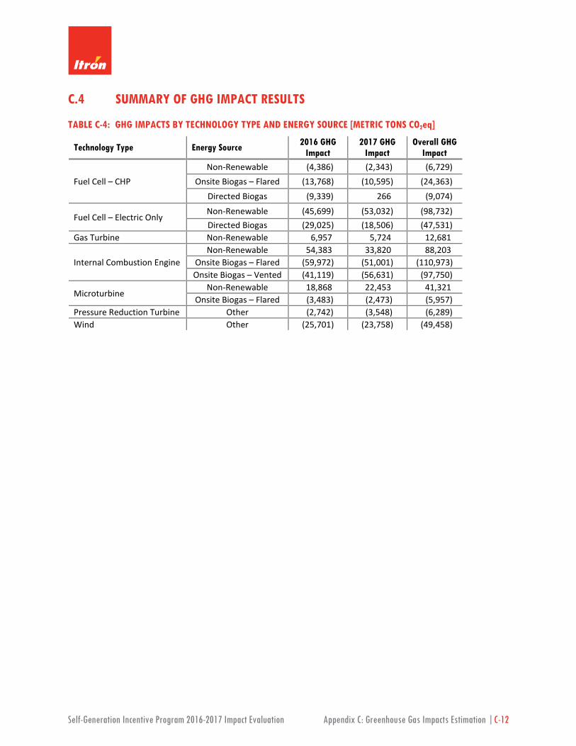
Self-Generation Incentive Program 2016-2017 Impact Evaluation Appendix C: Greenhouse Gas Impacts Estimation |C-12
C.4 SUMMARY OF GHG IMPACT RESULTS
TABLE C-4: GHG IMPACTS BY TECHNOLOGY TYPE AND ENERGY SOURCE [METRIC TONS CO2eq]
Technology Type Energy Source 2016 GHG Impact
2017 GHG Impact
Overall GHG Impact
Fuel Cell – CHP Non-Renewable (4,386) (2,343) (6,729)
Onsite Biogas – Flared (13,768) (10,595) (24,363) Directed Biogas (9,339) 266 (9,074)
Fuel Cell – Electric Only Non-Renewable (45,699) (53,032) (98,732) Directed Biogas (29,025) (18,506) (47,531)
Gas Turbine Non-Renewable 6,957 5,724 12,681
Internal Combustion Engine Non-Renewable 54,383 33,820 88,203
Onsite Biogas – Flared (59,972) (51,001) (110,973) Onsite Biogas – Vented (41,119) (56,631) (97,750)
Microturbine Non-Renewable 18,868 22,453 41,321
Onsite Biogas – Flared (3,483) (2,473) (5,957) Pressure Reduction Turbine Other (2,742) (3,548) (6,289) Wind Other (25,701) (23,758) (49,458)

Self-Generation Incentive Program 2016-2017 Impact Evaluation Appendix C: Greenhouse Gas Impacts Estimation |C-13
TABLE C-5: GHG IMPACTS BY PROGRAM ADMINISTRATOR AND TECHNOLOGY TYPE [METRIC TONS CO2eq]
PA Technology Type 2016 GHG Impact
2017 GHG Impact
Overall GHG Impact
CSE
Fuel Cell – CHP (9,402) (810) (10,212) Fuel Cell – Electric Only (6,821) (6,417) (13,238)
Gas Turbine 8,945 6,620 15,565
Internal Combustion Engine (1,906) (1,139) (3,045) Microturbine (99) (73) (172)
Pressure Reduction Turbine (1,523) (1,589) (3,112) Wind (1,784) (1,620) (3,405)
CSE Total (12,591) (5,029) (17,619)
PG&E
Fuel Cell – CHP (4,047) (977) (5,025) Fuel Cell – Electric Only (37,238) (24,404) (61,642)
Gas Turbine (191) 553 362 Internal Combustion Engine (62,116) (77,431) (139,547)
Microturbine 9,674 11,324 20,998 Pressure Reduction Turbine (887) (1,195) (2,081)
Wind (11,194) (10,677) (21,871) PG&E Total (105,999) (102,807) (208,806)
SCE
Fuel Cell – CHP (7,995) (5,889) (13,884) Fuel Cell – Electric Only (18,320) (26,900) (45,220)
Gas Turbine - - - Internal Combustion Engine 153 (3,827) (3,673)
Microturbine (267) 660 393 Pressure Reduction Turbine (331) (764) (1,096)
Wind (12,722) (11,461) (24,183) SCE Total (39,482) (48,181) (87,663)
SCG
Fuel Cell – CHP (6,048) (4,996) (11,044) Fuel Cell – Electric Only (12,345) (13,817) (26,163)
Gas Turbine (1,797) (1,449) (3,246) Internal Combustion Engine 17,160 8,585 25,745
Microturbine 6,076 8,069 14,145 Pressure Reduction Turbine - - -
Wind - - - SCG Total 3,045 (3,608) (562)
Program Total (155,027) (159,624) (314,651)

Self-Generation Incentive Program 2016-2017 Impact Evaluation Appendix D: Criteria Air Pollutant Impacts Estimation |D-1
APPENDIX D CRITERIA AIR POLLUTANT IMPACTS ESTIMATION METHODOLOGY AND RESULTS
This appendix describes the methodology used to estimate the impacts of criteria air pollutant emissions from the operation of Self-Generation Incentive Program (SGIP) projects. Criteria air pollutants are those air pollutants having national air quality standards with defined allowable concentrations in ambient air. Criteria air pollutants are carbon monoxide (CO), lead (Pb), oxides of nitrogen (NOX), ozone (O3), particulate matter (PM), and sulfur dioxide (SO2).1 Ozone is not directly generated by SGIP technologies and therefore ozone impacts are not reported.2 In addition, there is insufficient information on lead emissions to include an assessment of lead emission impacts. Criteria air pollutants considered in this analysis are limited to NOX and particulate matter in the 10-micron size range (PM10).
D.1 OVERVIEW
Criteria air pollutant impacts are estimated using an approach similar to the greenhouse gas (GHG) impacts estimation methodology described in Appendix C. Criteria air pollutant impacts are estimated as the difference between the emissions that occur from operation of SGIP projects and those that would occur from serving electrical, heating, and cooling loads via conventional energy services (i.e., the electricity grid, boilers, and electric chillers) in the absence of the SGIP. The principal difference between the GHG and criteria pollutant impacts methodologies is that the emissions from central station grid generation, boilers, and SGIP generators are not a simple function of the amount of gas consumed. For example, NOX emissions rates are a function of combustion stoichiometry and temperature, which can vary from one internal combustion engine to the next. In addition, post-combustion emission control technologies such as catalysts can significantly impact emissions rates. Emission control requirements can vary by air quality management district (AQMD) and program year (PY). This variability in potential emissions rates necessitates the development of emissions rate estimates that are specific to a given technology, program year, and energy source.
The sections below describe the overall approach and assumptions made in estimating emissions rates for each of the criteria air pollutants treated.
D.2 OXIDES OF NITROGEN (NOX) EMISSION RATES
The rate at which NOX is created is a function of the energy source, the combustion process/chemical reaction, and the type of emissions control technology installed. All fuel-consuming SGIP technologies
1 Environmental Protection Agency, from https://www.epa.gov/criteria-air-pollutants 2 Ozone or oxidant makes up photochemical smog and NOX emissions are critical precursors to the formation of
oxidant.

Self-Generation Incentive Program 2016-2017 Impact Evaluation Appendix D: Criteria Air Pollutant Impacts Estimation |D-2
generate NOX emissions. Sources of avoided NOX emissions include central-station grid power plants, natural gas boilers, and biogas flares.
SGIP Project NOX Emission Rates
NOX emission rates from SGIP projects are based on literature research and personal communications with industry experts conducted by Itron. The amount of NOX produced by each technology type can vary by program year, primary due to changes in air emission requirements imposed by the California Air Resources Board (CARB) and improvements in Best Available Control Technology (BACT). Studies conducted in the 2000 to 2005 timeframe indicated that widespread adoption of distributed generation (DG) technologies could potentially lead to a degradation of air quality due to increased emissions of NOX from DG systems.3,4 Leading into 2000, many of the DG systems operating in California were fueled by diesel and had relatively high NOX emissions. A 2006 survey of air quality management district regulations on NOX controls for natural gas-fired reciprocating engines found NOX requirements ranged from 0.3 lb/MWh in the South Coast AQMD to over 4 lb/MWh.5 Due to concerns over potential increases in NOX emissions from DG resources, the Legislature passed Senate Bill 1298 (Bowen/Peace) in September 2000.6 SB 1298 directed by CARB to develop an air pollution control certification program for DG technologies by January 2003. The CARB certification had a phase-in approach that required increasingly lower NOX emissions between 2005 and 2007.
Table D-1 lists the NOX emission rates used to estimate 2016-2017 emissions from SGIP technologies.
3 Ianucci, J., Horgan, S., Eyer, J., Cibulka, L., 2000. “Air pollution emissions impacts associated with the economic
market potential of distributed generation in California,” Distributed Utility Associates, prepared for The California Air Resources Board, Contract #97-326.
4 California Institute for Energy and Environment, “Impacts of Distributed Generation on Air Quality: A Roadmap,” prepared for the California Energy Commission, CEC-500-2008-022, June 2008
5 SMUD, “Small Engine Emission Reduction for Dairy Digesters,” prepared by Itron, November 2006 6 http://leginfo.ca.gov/pub/99-00/bill/sen/sb_1251-1300/sb_1298_bill_20000927_chaptered.html

Self-Generation Incentive Program 2016-2017 Impact Evaluation Appendix D: Criteria Air Pollutant Impacts Estimation |D-3
TABLE D-1: NOX EMISSION RATES FOR SGIP TECHNOLOGIES
Technology Type Program Year Energy Source NOX Emission Rate [lb NOX/MWh]
Fuel Cell – CHP All All 0.010 Fuel Cell – Electric Only All All 0.002
Gas Turbine PY01-PY06 All 0.300
PY07 All 0.070 PY08-PY17 All 0.070
Internal Combustion Engine & Microturbine
PY01-PY06 All 0.200 PY07 All 0.135
PY08-PY17 All 0.070
Due to their chemistry, fuel cells tend to have significantly lower NOX emissions rates compared to combustion technologies. Prior to PY07, before stringent NOX control rules went into effect, combustion technologies had the highest NOX emission rates. All combustion technologies that applied after PY07 are assumed to meet CARB’s 0.070 lb / MWh target. During PY07, combustion technologies were eligible for SGIP incentives if they met the CARB’s NOX target either through emission controls or by using a combined heat and power (CHP) offset due to avoided boiler use. Consequently, it cannot be assumed that all PY07 combustion technologies achieved CARB’s emissions targets. Instead, PY07 is treated as a transition year for internal combustion engines and microturbines; their average emission rate is assumed to be half way between the PY01-PY06 rate and the CARB 0.070 lb / MWh target. This is a proxy for an assumption that half the projects achieved CARB’s target through emissions controls and the other half achieved CARB’s target via CHP credits. PY07 gas turbines are assumed to have met CARB’s NOX target using emission controls.
Baseline NOX Emission Rates
Central station power plants and on-site boilers all generate NOX as a result of the combustion of natural gas. Biogas flares also generate NOX as a result of the combustion of biogas.
Central Station Power Plant NOX Emission Rates
NOX emissions rates from central station power plants are based on Energy and Environmental Economics’ (E3’s) Avoided Cost Calculator assumptions.
Boiler and Flare NOX Emission Rates
NOX emission rates from natural gas boilers and biogas flares are based on literature research conducted by Itron. In most urban areas in California, air pollution control districts passed regulations in the mid-1990’s requiring some form of NOX control on commercial sized boilers (i.e., boilers in the size range of less than 10 MMBtu heat input up to about 50 MMBtu heat input). In these urban areas (e.g., Bay Area,

Self-Generation Incentive Program 2016-2017 Impact Evaluation Appendix D: Criteria Air Pollutant Impacts Estimation |D-4
Southern California, San Diego), the regulations required control of NOX to 30 parts per million by volume (ppmv) at 3% O2.7 This corresponds to approximately 0.037 lb of NOX /MMBtu heat input. In non-urban areas of California, boilers were left to meet new source performance standards (NSPS) requirements.
This analysis assumes that two thirds of SGIP projects are in urban areas with the remaining third in non-urban areas and that the average boiler NOX emission rate can be approximated by the following equation:
𝑁𝑁𝑂𝑂𝑋𝑋,𝑏𝑏𝑏𝑏𝑏𝑏𝑏𝑏𝑏𝑏𝑏𝑏 = 23
× 0.037 𝑏𝑏𝑏𝑏𝑀𝑀𝑀𝑀𝑀𝑀𝑀𝑀𝑀𝑀
+ 13
× 0.190 𝑏𝑏𝑏𝑏𝑀𝑀𝑀𝑀𝑀𝑀𝑀𝑀𝑀𝑀
= 0.088 𝑏𝑏𝑏𝑏𝑀𝑀𝑀𝑀𝑀𝑀𝑀𝑀𝑀𝑀
EQUATION D-1
Table D-2 lists the NOX emission rates used to estimate 2016-2017 emissions from baseline natural gas boilers and biogas flares.
TABLE D-2: NOX EMISSION RATES FOR NATURAL GAS BOILERS AND BIOGAS FLARES
Baseline Component NOX Emission Rate [lb NOX/MWh]
Natural Gas Boiler 0.088 Biogas Flare 0.056
Venting for biogas to the atmosphere does not produce NOX, therefore, there is no avoided NOX component for projects that would have otherwise vented biogas.
D.3 PARTICULATE MATTER EMISSION RATES
Particulate matter is a complex mixture of extremely small particles and liquid droplets. The size of particles is directly linked to their potential for causing health problems. The Environmental Protection Agency (EPA) is concerned about particles that are 10 micrometers in diameter or smaller because those are the particles that generally pass through the throat and nose and enter the lungs.8 Once inhaled, these particles can affect the heart and lungs and cause serious health effects.9 As with NOX, the rate at which PM10 is created is a function of the energy source, the combustion process/chemical reaction, and the types of emissions controls installed. All fuel-consuming SGIP technologies generate PM10 emissions. Sources of avoided PM10 emissions include central-station grid power plants, natural gas boilers, and biogas flares.
7 Bay Area Air Quality Management District, “BAAQMD Regulation 9, Rule 7: Nitrogen Oxides and Carbon
Monoxide from Industrial, Institutional and Commercial Boilers, Steam Generators and Process Heaters, May 2007
8 This report only examines particulate matter between 2.5 and 10 micrometers in diameter. 9 https://www.epa.gov/pm-pollution

Self-Generation Incentive Program 2016-2017 Impact Evaluation Appendix D: Criteria Air Pollutant Impacts Estimation |D-5
SGIP Project PM10 Emission Rates
PM10 emissions rates from SGIP projects are based on literature research and personal communications with industry experts conducted by Itron staff. Table D-3 lists the PM10 emission rates used to estimate 2016 – 2017 emissions from SGIP projects.
TABLE D-3: PM10 EMISSION RATES FOR SGIP TECHNOLOGIES
Technology Type Program Year Energy Source PM10 Emission Rate [lb PM10 /MWh]
Fuel Cell – CHP or Electric Only All All 0.00002 Gas Turbine All Natural Gas 0.05635
Internal Combustion Engine All Natural Gas 0.06006 All Biogas 0.06969
Microturbine All All 0.08575
As with NOX, fuel cells have the lowest PM10 emissions rates when compared to combustion technologies.
Baseline PM10 Emission Rates
Central station power plants and on-site boilers all generate PM10 as a result of the combustion of natural gas. Biogas flares also generate PM10 as a result of the combustion of biogas.
Central Station Power Plant PM10 Emission Rates
PM10 emissions rates from central station power plants are based on E3’s Avoided Cost Calculator assumptions.
Boiler and Flare PM10 Emission Rates
PM10 emission rates from natural gas boilers and biogas flares are based on literature research conducted by Itron. Table D-4 lists the PM10 emission rates used to estimate 2016 – 2017 emissions from natural gas boilers and biogas flares.
TABLE D-4: PM10 EMISSION RATES FOR NATURAL GAS BOILERS AND BIOGAS FLARES
Baseline Component PM10 Emission Rate [lb PM10 /MWh]
Natural Gas Boiler 0.00773 Biogas Flare 0.01418

Self-Generation Incentive Program 2016-2017 Impact Evaluation Appendix D: Criteria Air Pollutant Impacts Estimation |D-6
Venting of biogas to the atmosphere does not produce PM10, therefore, there is no avoided PM10 component for projects that would have otherwise vented biogas.
D.4 EMISSIONS IMPACT CALCULATIONS
Criteria pollutant impacts are calculated as the annual sum of hourly SGIP project emissions minus the annual sum of hourly electric power plant emissions, natural gas boiler emissions, and biogas flare emissions for all projects.
∆𝐶𝐶𝐶𝐶𝑏𝑏,ℎ = 𝑠𝑠𝑠𝑠𝑠𝑠𝑠𝑠𝐶𝐶𝐶𝐶𝑏𝑏,ℎ − �𝑏𝑏𝑏𝑏𝑠𝑠𝑏𝑏𝐶𝐶𝑠𝑠𝑏𝑏𝑏𝑏𝑠𝑠𝑏𝑏𝐶𝐶𝐶𝐶𝑏𝑏,ℎ + 𝑏𝑏𝑏𝑏𝑠𝑠𝑏𝑏𝐶𝐶𝑠𝑠𝐶𝐶ℎ𝑠𝑠𝑖𝑖𝑖𝑖𝑏𝑏𝑖𝑖𝐶𝐶𝐶𝐶𝑏𝑏,ℎ + 𝑏𝑏𝑏𝑏𝑠𝑠𝑏𝑏𝑏𝑏𝑖𝑖𝑖𝑖𝐶𝐶𝐶𝐶𝑏𝑏,ℎ + 𝑏𝑏𝑏𝑏𝑠𝑠𝑏𝑏𝑏𝑏𝑠𝑠𝑏𝑏𝐶𝐶𝐶𝐶𝑏𝑏,ℎ� EQUATION D-2
Where: ΔCPi,h = Criteria pollutant Impact for SGIP project i during project h [lb/hour]
Each component of the criteria pollutant impacts calculation is further described below.
SGIP Project Emissions
𝑠𝑠𝑠𝑠𝑠𝑠𝑠𝑠𝐶𝐶𝐶𝐶𝑏𝑏,ℎ = 𝑏𝑏𝑏𝑏𝑠𝑠𝑏𝑏ℎ𝑖𝑖𝑏𝑏,ℎ × 𝑠𝑠𝑠𝑠𝑠𝑠𝑠𝑠𝐶𝐶𝐶𝐶𝑠𝑠𝑏𝑏𝑠𝑠𝑏𝑏𝑏𝑏 × 1 𝑀𝑀𝑀𝑀ℎ
1,000 𝑘𝑘𝑀𝑀ℎ EQUATION D-3
Where: sgipCPi,h = Specific criteria pollutant emitted by SGIP project i during project h
[lb/hour] engohri,h = Electrical output of SGIP project i during project h based on metered data
collected from SGIP projects net any parasitic losses [kWh] sgipCPRatei = Criteria pollutant emissions rate for SGIP project i during project h as
defined in section D.2 (NOX) and D.3 (PM10) [lb/MWh]

Self-Generation Incentive Program 2016-2017 Impact Evaluation Appendix D: Criteria Air Pollutant Impacts Estimation |D-7
Baseline Power Plant Emissions
The baseline power plant criteria pollutant emission rate, when multiplied by the quantity of electricity generated for each baseline scenario, estimates the hourly emissions avoided from central station power plants.
𝑏𝑏𝑏𝑏𝑠𝑠𝑏𝑏𝐶𝐶𝑠𝑠𝐶𝐶ℎ𝑠𝑠𝑖𝑖𝑖𝑖𝑏𝑏𝑖𝑖𝐶𝐶𝐶𝐶𝑏𝑏,ℎ = 𝑠𝑠𝑏𝑏𝑝𝑝𝑏𝑏𝑖𝑖𝐶𝐶𝑖𝑖𝑏𝑏𝑏𝑏𝑠𝑠𝐶𝐶𝐶𝐶𝑠𝑠𝑏𝑏𝑠𝑠𝑏𝑏ℎ × 𝑐𝑐ℎ𝑖𝑖𝑖𝑖𝑏𝑏𝑖𝑖𝑏𝑏𝑐𝑐𝑏𝑏,ℎ × 1 𝑀𝑀𝑀𝑀ℎ1,000 𝑘𝑘𝑀𝑀ℎ
EQUATION D-4
𝑏𝑏𝑏𝑏𝑠𝑠𝑏𝑏𝐶𝐶𝑠𝑠𝑏𝑏𝑏𝑏𝑠𝑠𝑏𝑏𝐶𝐶𝐶𝐶𝑏𝑏,ℎ = 𝑠𝑠𝑏𝑏𝑝𝑝𝑏𝑏𝑖𝑖𝐶𝐶𝑖𝑖𝑏𝑏𝑏𝑏𝑠𝑠𝐶𝐶𝐶𝐶𝑠𝑠𝑏𝑏𝑠𝑠𝑏𝑏ℎ × 𝑏𝑏𝑏𝑏𝑠𝑠𝑏𝑏ℎ𝑖𝑖𝑏𝑏,ℎ × 1 𝑀𝑀𝑀𝑀ℎ1,000 𝑘𝑘𝑀𝑀ℎ
EQUATION D-5
Where: basePpChillerCPi,h = Baseline power plant criteria pollutant emissions avoided due to
SGIP project i delivery of cooling services during project h [lb/hour]
basePpEngoCPi,h = Baseline power plant criteria pollutant emissions avoided due to SGIP project i during project h [lb/hour]
powerPlantCPRateh = Baseline power plant criteria pollutant emissions rate as defined in section D.2 (NOX) and D.3 (PM10) [lb/MWh]
chlrEleci,h = the electricity of a power plant that would be needed to provide baseline electric chiller for SGIP CHP project i for hour h, as defined in Appendix C [kWh]
Baseline Boiler Emissions
Baseline natural gas boiler criteria pollutant emissions are calculated based upon hourly useful heat recovery values for the SGIP CHP project as follows:
𝑏𝑏𝑏𝑏𝑠𝑠𝑏𝑏𝑏𝑏𝑖𝑖𝑖𝑖𝐶𝐶𝐶𝐶𝑏𝑏,ℎ = 𝐻𝐻𝑏𝑏𝐻𝐻𝐻𝐻𝐻𝐻𝑁𝑁𝐺𝐺𝑏𝑏,ℎ × 1𝑏𝑏𝑒𝑒𝑒𝑒𝑀𝑀𝑏𝑏𝑏𝑏
× 𝑏𝑏𝑖𝑖𝑖𝑖𝐶𝐶𝐶𝐶𝑠𝑠𝑏𝑏𝑠𝑠𝑏𝑏 × 1 𝑀𝑀𝑀𝑀ℎ1,000 𝑘𝑘𝑀𝑀ℎ
EQUATION D-6
Where: baseBlrCPi,h = Criteria pollutant emissions of the baseline natural gas boiler for SGIP
CHP project i for hour h [lb/hour] HEATINGi,h = Heating services provided by SGIP CHP project i for hour h [MBtu] effBlr = 0.8 - assumed efficiency of the baseline natural boiler, based on -
previous cost effectiveness evaluations [Mbtuout/Mbtuin]
baseBlrCPi,h = Criteria pollutant emissions rate of baseline natural gas boilers as defined in section D.2 (NOX) and D.3 (PM10) [lb/MWh]
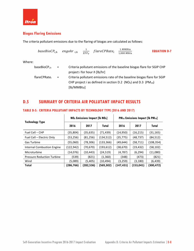
Self-Generation Incentive Program 2016-2017 Impact Evaluation Appendix D: Criteria Air Pollutant Impacts Estimation |D-8
Biogas Flaring Emissions
The criteria pollutant emissions due to the flaring of biogas are calculated as follows:
𝑏𝑏𝑏𝑏𝑠𝑠𝑏𝑏𝑏𝑏𝑠𝑠𝑏𝑏𝐶𝐶𝐶𝐶𝑏𝑏,ℎ = 𝑏𝑏𝑏𝑏𝑠𝑠𝑏𝑏ℎ𝑖𝑖(𝑏𝑏,ℎ) × 1𝐸𝐸𝐸𝐸𝐸𝐸𝑇𝑇
× 𝑓𝑓𝑖𝑖𝑏𝑏𝑖𝑖𝑏𝑏𝐶𝐶𝐶𝐶𝑠𝑠𝑏𝑏𝑠𝑠𝑏𝑏𝑏𝑏 × 1 𝑀𝑀𝑀𝑀𝑀𝑀𝑀𝑀𝑀𝑀1,000 𝑀𝑀𝑏𝑏𝑀𝑀𝑀𝑀
EQUATION D-7
Where: baseBioCPi,h = Criteria pollutant emissions of the baseline biogas flare for SGIP CHP
project i for hour h [lb/hr] flareCPRatei = Criteria pollutant emissions rate of the baseline biogas flare for SGIP
CHP project i as defined in section D.2 (NOX) and D.3 (PM10) [lb/MMBtu]
D.5 SUMMARY OF CRITERIA AIR POLLUTANT IMPACT RESULTS
TABLE D-5: CRITERIA POLLUTANT IMPACTS BY TECHNOLOGY TYPE (2016 AND 2017)
Technology Type NOX Emissions Impact [lb NOX] PM10 Emissions Impact [lb PM10]
2016 2017 Total 2016 2017 Total
Fuel Cell – CHP (35,804) (35,635) (71,439) (14,950) (16,215) (31,165) Fuel Cell – Electric Only (53,256) (81,256) (134,512) (35,775) (48,737) (84,512) Gas Turbine (55,060) (78,306) (133,366) (49,644) (58,711) (108,354) Internal Combustion Engine (122,942) (70,670) (193,612) (38,670) (19,432) (58,102)
Microturbine (14,076) (10,443) (24,519) (4,787) (6,294) (11,080) Pressure Reduction Turbine (539) (821) (1,360) (348) (473) (821) Wind (5,089) (5,405) (10,494) (3,259) (3,180) (6,439) Total (286,766) (282,536) (569,302) (147,431) (153,041) (300,472)

Self-Generation Incentive Program 2016-2017 Impact Evaluation Appendix D: Criteria Air Pollutant Impacts Estimation |D-9
TABLE D-6: CRITERIA POLLUTANT IMPACTS BY ENERGY SOURCE (2016 AND 2017)
Energy Source NOX Emissions Impact [lb NOX] PM10 Emissions Impact [lb PM10]
2016 2017 Total 2016 2017 Total
Non-Renewable (151,189) (170,169) (321,358) (110,719) (120,609) (231,327)
Onsite Biogas (119,716) (88,940) (208,656) (26,027) (18,362) (44,389)
Directed Biogas (10,232) (17,201) (27,433) (7,079) (10,418) (17,497)
Other (5,628) (6,226) (11,854) (3,606) (3,653) (7,259)
Total (286,766) (282,536) (569,302) (147,431) (153,041) (300,472)
Self-Generation Incentive Program 2016-2017 Impact Evaluation Appendix E: Sources of Uncertainty and Results|E-1
APPENDIX E SOURCES OF UNCERTAINTY AND RESULTS This appendix provides an assessment of the uncertainty associated with Self-Generation Incentive Program (SGIP) impacts estimates for generation technologies. Program impacts discussed include those on energy (electricity, fuel, and heat), as well as those on greenhouse gas (GHG) emissions. The principal factors contributing to uncertainty in the results reported for these two types of program impacts are quite different. The treatment of those factors is described below for each of the two types of impacts.
Generation project uncertainty estimates are provided for annual and peak electrical impacts.
E.1 OVERVIEW OF ENERGY IMPACTS UNCERTAINTY
Electricity, fuel, and useful heat recovery impacts estimates are affected by at least two sources of error that introduce uncertainty into the population-level estimates: measurement error and sampling error. Measurement error refers to the differences between actual values (e.g., actual electricity production) and measured values (i.e., electricity production values recorded by metering and data collection systems). Sampling error refers to differences between actual values and values estimated for unmetered systems. The estimated impacts calculated for unmetered systems are based on the assumption that performance of unmetered systems is identical to the average performance exhibited by groups of similar metered projects. Very generally, the central tendency (i.e., an average) of metered systems is used as a proxy for the central tendency of unmetered systems.
The actual performance of unmetered systems is not known, and will never be known. It is, therefore, not possible to directly assess the validity of the assumption regarding identical central tendencies. However, it is possible to examine this issue indirectly by incorporating information about the performance variability characteristics of the systems.
Theoretical and empirical approaches exist to assess uncertainty effects attributable to both measurement and sampling error. Propagation of error equations are a representative example of theoretical approaches. Empirical approaches to quantification of impact estimate uncertainty are not grounded on equations derived from theory. Instead, information about factors contributing to uncertainty is used to create large numbers of possible sets of actual values for unmetered systems. Characteristics of the sets of simulated actual values are analyzed. Inferences about the uncertainty in impacts estimates are based on results of this analysis.
For this impacts evaluation an empirical approach known as Monte Carlo Simulation (MCS) analysis was used to quantify impacts estimates uncertainty. The term MCS refers to “the use of random sampling techniques and often the use of computer simulation to obtain approximate solutions to mathematical or

Self-Generation Incentive Program 2016-2017 Impact Evaluation Appendix E: Sources of Uncertainty and Results|E-2
physical problems especially in terms of a range of values each of which has a calculated probability of being the solution.”1
A principle advantage of this approach is that it readily accommodates complex analytical questions. This is an important advantage for this evaluation because numerous factors contribute to variability in impacts estimates, and the availability of metered data upon which to base impact estimates is variable. For example, metered electricity production and heat recovery data are both available for some cogeneration systems, whereas other systems may also include metered fuel consumption, while still others might have combinations of data available.
E.2 OVERVIEW OF GREENHOUSE GAS IMPACTS UNCERTAINTY
Electricity and fuel impacts estimates represent the starting point for the analysis of GHG emission impacts; thus, uncertainty in those electricity and fuel impacts estimates flows down to the GHG emissions impact estimates. However, additional sources of uncertainty are introduced in the course of the GHG emissions impact analysis. GHG emissions impact estimates are, therefore, subject to greater levels of uncertainty than are electricity and fuel impact estimates. The two most important additional sources of uncertainty in GHG emissions impacts are summarized below.
E.2.1 Baseline Central Station Power Plant GHG Emissions
Estimation of GHG emission impacts for each SGIP project involves comparison of emissions of the SGIP project with emissions that would have occurred in the absence of the program. The latter quantity depends on the central station power plant generation technology (e.g., natural gas combined cycle, natural gas turbine) that would have met the participant’s electric load if the SGIP project had not been installed. Data concerning marginal baseline generation technologies and their efficiencies (and, hence, GHG emissions factors) were obtained from Energy + Environmental Economics (E3). Quantitative assessment of uncertainty in E3’s avoided GHG emissions rates is outside the scope of this SGIP impacts evaluation.
E.2.2 Baseline Biogas Project GHG Emissions
Biomass material (e.g., trash in landfills, manure in dairies) would typically have existed and decomposed (releasing methane (CH4)), even in the absence of the program. While the program does not influence the existence or decomposition of the biomass material, it may impact whether or not the CH4is released
1 Webster’s dictionary.

Self-Generation Incentive Program 2016-2017 Impact Evaluation Appendix E: Sources of Uncertainty and Results|E-3
directly into the atmosphere. This is critical because CH4is a much more active GHG than are the products of its combustion (e.g., CO2).
The CH4 disposition baseline assumptions used in this GHG impact evaluation are summarized in Table E-1. A more detailed treatment of biogas baseline assumptions is included in Appendix C.
TABLE E-1: METHANE DISPOSITION BASELINE ASSUMPTIONS FOR BIOGAS PROJECTS
Renewable Fuel Facility Type Methane Disposition Baseline Assumption
Dairy Digester Venting Waste Water Treatment
Flaring Landfill Gas Recovery
Directed Biogas
Due to the influential nature of this factor, and given the current relatively high level of uncertainty surrounding assumed baselines, this evaluation continues to incorporate site-specific information about CH4 disposition into impacts analyses.
E.3 SOURCES OF DATA FOR UNCERTAINTY ANALYSIS
The usefulness of MCS results rests on the degree to which the factors underlying the simulations of actual performance of unmetered systems resemble factors known to influence those SGIP projects for which impacts estimates are being reported. Several key sources of data for these factors are described briefly below.
E.3.1 SGIP Project Information
Basic project identifiers include PA, payment status, project location, technology type, fuel type, and project size. This information is obtained from the statewide database maintained by the Program Administrators (PAs). More detailed project information (e.g., heat exchanger configuration) is obtained from site inspection verification reports developed by the PAs or their consultants just prior to issuance of incentive payments.
E.3.2 Metered Data for SGIP Projects
Collection and analysis of metered performance data for SGIP projects is a central focus of the overall program evaluation effort. In the MCS study, the metered performance data are used for two principal purposes:

Self-Generation Incentive Program 2016-2017 Impact Evaluation Appendix E: Sources of Uncertainty and Results|E-4
Metered data are used to estimate the actual performance of metered systems. The metered data are not used directly for this purpose. Rather, information about measurement error is applied to metered values to estimate actual values.
The variability characteristics exhibited by groups of metered data contribute to development of distributions used in the MCS study. Values from the distributions are randomly picked to estimate the performance of unmetered systems in large numbers of simulation runs to explore the likelihood that actual total performance of groups of unmetered systems deviates by certain amounts from estimates of their performance.
E.3.3 Manufacturer’s Technical Specifications
Metering systems are subject to measurement error. The values recorded by metering systems represent very close approximations to actual performance; they are not necessarily identical to actual performance. Technical specifications available for metering systems provide information necessary to characterize the difference between measured and actual performance.
E.4 UNCERTAINTY ANALYSIS ANALYTICAL METHODOLOGY
The analytic methodology used for the MCS study is described in this section. The discussion is broken down into five steps:
Ask Question,
Design Study,
Generate Sample Design,
Calculate the Quantities of Interest for Each Sample, and
Analyze Accumulated Quantities of Interest.
E.4.1 Ask Question
The first step in the MCS study is to clearly describe the question(s) that the MCS study was designed to answer. In this instance, that question is: How confident can one be that actual program total impact deviates from reported program total impact by less than certain amounts? The scope of the MCS study includes the following program total impacts:
Program Total Annual Electrical Energy Impacts,
Program Total Coincident Peak Electrical Demand Impacts, and
Program Total System Efficiency.

Self-Generation Incentive Program 2016-2017 Impact Evaluation Appendix E: Sources of Uncertainty and Results|E-5
E.4.2 Design Study
The MCS study’s design determines requirements for generation of sample data. The process of specifying study design includes making tradeoffs between flexibility, accuracy, and cost. This MCS study’s tradeoffs pertain to treatment of the dynamic nature of the SGIP and to treatment of the variable nature of data availability. Some of the projects came online during 2017 and, therefore, contributed to energy impacts for only a portion of the year. Some of the projects for which metered data are available have gaps in the metered data archive that required estimation of impacts for a portion of hours during 2016 and 2017. These issues are discussed below.
Sample data for each month of the year could be simulated, and then annual electrical energy impacts could be calculated as the sum of the monthly impacts. Alternatively, sample energy production data for entire years could be generated. An advantage of the monthly approach is that it accommodates systems that came online during 2017, and, therefore, contributed to energy impacts for only a portion of the year. The disadvantage of using monthly simulations is that this approach is 12 times more processor-intensive than an annual simulation approach.
A central element of the MCS study involves generation of actual performance values (i.e., sample data) for each simulation run. The method used to generate these values depends on whether or not the project is metered. However, for many of the SGIP projects, metered data are available for a portion – but not all – of 2016 and 2017. This complicates any analysis that requires classification of projects as either “metered” or “not metered.”
An effort was made to accommodate the project status and data availability details described above without consuming considerable time and resources. To this end, two important simplifying assumptions are included in the MCS study design.
Each data archive (e.g., electricity, fuel consumption, useful heat recovery) for each month for each project is classified as being either “metered” (at least 90% of any given month’s reported impacts are based on metered data) or “unmetered” (less than 90% of any given month’s reported impacts are based on metered data) for MCS purposes.
An operations status of “Normal” or “Unknown” was assigned to each month for each unmetered system based on a telephone survey of participants.2
2 This research primarily involved contacting site hosts to determine the operational status of unmetered
systems. More details are provided in Appendix B.

Self-Generation Incentive Program 2016-2017 Impact Evaluation Appendix E: Sources of Uncertainty and Results|E-6
E.4.3 Generate Sample Data
Actual values for each of the program impact estimates identified above (“Ask Question”) are generated for each sample (i.e., “run” or simulation).
If metered data are available for the project, then the actual values are created by applying a measurement error to the metered values. If metered data are not available for the project, the actual values are created using distributions that reflect performance variability assumptions. A total of 1,000 simulation runs were used to generate sample data.
Metered Data Available – Generating Sample Data that Include Measurement Error
The assumed characteristics of random measurement-error variables are summarized in Table E-2. The ranges are based on typical accuracy specifications from manufacturers of metering equipment (e.g., specified accuracy of +/- 2%). A uniform distribution with mean equal to zero is assumed for all three measurement types. This distribution implies that any error value within the stated range has an identical probability of occurring in any measurement. This distribution is more conservative than some other commonly assumed distributions (e.g., normal “bell-shaped” curve) because the outlying values are just as likely to occur as the central values.
TABLE E-2: SUMMARY OF RANDOM MEASUREMENT ERROR VARIABLES
Measurement Range Mean Distribution
Electrical Generation -0.5% to 0.5% 0% Uniform Fuel Consumption -2% to 2%
Useful Heat Recovered -5% to 5%
Metered Data Unavailable – Generating Sample Data from Performance Distributions
In the case of unmetered projects, the sample data are generated by random assignment from distributions of performance values assumed representative of entire groups of unmetered projects. Because measured performance data are not available for any of these projects, the natural place to look first for performance values is similar metered projects.
Specification of performance distributions for the MCS study involves a degree of judgment in at least two areas. The first is in deciding whether or not metered data available for a stratum are sufficient to provide a realistic indication of the distribution of values likely for the unmetered projects. The second is when metered data available for a stratum are not sufficient in deciding when and how to incorporate the metered data available for other strata into a performance distribution for the data-insufficient stratum.

Self-Generation Incentive Program 2016-2017 Impact Evaluation Appendix E: Sources of Uncertainty and Results|E-7
Table E-3 shows the groups used to estimate the uncertainty in the California Independent System Operator (CAISO) peak hour impact.
TABLE E-3: PERFORMANCE DISTRIBUTIONS DEVELOPED FOR THE 2016 AND 2017 CAISO PEAK HOUR MCS ANALYSIS
Technology Type Energy Source PA
Fuel Cell – Combined Heat and Power Non-renewable, Renewable
All
Fuel Cell – Electric only All Gas Turbine Non-renewable
Internal Combustion Engine Non-renewable, Renewable Microturbine Non-renewable, Renewable Wind All
Table E-4 shows the groups used to estimate the uncertainty in the yearly energy production. Internal combustion engines, gas turbines, and microturbines are grouped together for the uncertainty analysis of the annual energy production because of the small number of systems within each technology group for which data were available for 90% of each month in the year.
TABLE E-4: PERFORMANCE DISTRIBUTIONS DEVELOPED FOR THE 2016 AND 2017 ANNUAL ENERGY PRODUCTIONS MCS ANALYSIS
Technology Type Energy Source PA
Fuel Cell – Combined Heat and Power All
All
Fuel Cell – Electric only All Gas Turbine All Internal Combustion Engine/ Microturbine Non-renewable, Renewable
Pressure Reduction Turbine All Wind All
Performance Distributions for Coincident Peak Impacts
Performance distributions were developed for each of the groups in Table E-3 and Table E-4 based on metered data and engineering judgment. In the MCS, a capacity factor is randomly assigned from the performance distribution and sample values are calculated as the product of the capacity factor and system size. All of these performance distributions are shown in Figure E-1 through Figure E-10.

Self-Generation Incentive Program 2016-2017 Impact Evaluation Appendix E: Sources of Uncertainty and Results|E-8
FIGURE E-1: MCS DISTRIBUTION – CHP FUEL CELL COINCIDENT PEAK OUTPUT (NON-RENEWABLE FUEL)
FIGURE E-2: MCS DISTRIBUTION – CHP FUEL CELL COINCIDENT PEAK OUTPUT (RENEWABLE FUEL)
FIGURE E-3: MCS DISTRIBUTION – ELECTRIC-ONLY FUEL CELL COINCIDENT PEAK OUTPUT (ALL FUEL)
FIGURE E-4: MCS DISTRIBUTION – GAS TURBINE COINCIDENT PEAK OUTPUT (NON-RENEWABLE FUEL)
FIGURE E-5: MCS DISTRIBUTION – INTERNAL COMBUSTION ENGINE COINCIDENT PEAK OUTPUT (NON-RENEWABLE FUEL)
FIGURE E-6: MCS DISTRIBUTION – INTERNAL COMBUSTION ENGINE COINCIDENT PEAK OUTPUT (RENEWABLE FUEL)

Self-Generation Incentive Program 2016-2017 Impact Evaluation Appendix E: Sources of Uncertainty and Results|E-9
FIGURE E-7: MCS DISTRIBUTION – MICROTURBINE COINCIDENT PEAK OUTPUT (NON-RENEWABLE FUEL)
FIGURE E-8: MCS DISTRIBUTION – MICROTURBINE COINCIDENT PEAK OUTPUT (RENEWABLE FUEL)
FIGURE E-9: MCS DISTRIBUTION – PRT COINCIDENT PEAK OUTPUT
FIGURE E-10: MCS DISTRIBUTION – WIND TURBINE COINCIDENT PEAK OUTPUT
Performance Distributions for Energy Impacts
Performance distributions used to generate sample data for annual energy impacts are shown in Figure E-11 through Figure E-17.

Self-Generation Incentive Program 2016-2017 Impact Evaluation Appendix E: Sources of Uncertainty and Results|E-10
FIGURE E-11: MCS DISTRIBUTION – ENGINE/COMBUSTION TURBINE (NON-RENEWABLE) ENERGY PRODUCTION (CAPACITY FACTOR)
FIGURE E-12: MCS DISTRIBUTION – ENGINE/COMBUSTION TURBINE (RENEWABLE) ENERGY PRODUCTION (CAPACITY FACTOR)
FIGURE E-13: MCS DISTRIBUTION – CHP FUEL CELL (ALL FUEL) ENERGY PRODUCTION (CAPACITY FACTOR)
FIGURE E-14: MCS DISTRIBUTION – ELECTRIC-ONLY FUEL CELL (ALL FUEL) ENERGY PRODUCTION (CAPACITY FACTOR)

Self-Generation Incentive Program 2016-2017 Impact Evaluation Appendix E: Sources of Uncertainty and Results|E-11
FIGURE E-15: MCS DISTRIBUTION – GAS TURBINE (NON-RENEWABLE) ENERGY PRODUCTION (CAPACITY FACTOR)
FIGURE E-16: MCS DISTRIBUTION – PRESSURE REDUCTION TURBINE ENERGY PRODUCTION (CAPACITY FACTOR)
FIGURE E-17: MCS DISTRIBUTION – WIND TURBINE ENERGY PRODUCTION (CAPACITY FACTOR)
Figure E-18 through Figure E-20 display the performance distributions used to generate sample data for heat recovery rates.

Self-Generation Incentive Program 2016-2017 Impact Evaluation Appendix E: Sources of Uncertainty and Results|E-12
FIGURE E-18: MCS DISTRIBUTION – ENGINE/COMBUSTION TURBINE HEAT RECOVERY RATE (MBTU/KWH)
FIGURE E-19: MCS DISTRIBUTION – CHP FUEL CELL HEAT RECOVERY RATE (MBTU/KWH)
FIGURE E-20: MCS DISTRIBUTION – GAS TURBINE HEAT RECOVERY RATE (MBTU/KWH)
E.4.4 Bias
Performance data collected from metered projects were used to estimate program impacts attributable to unmetered projects. If the metered projects are not representative of the unmetered projects, then those estimates will include systematic errors called bias. Potential sources of bias of principal concern for this study include:
Planned Data Collection Disproportionally Favors Dissimilar Groups
Useful heat recovery metering is typically installed on projects that are still under their contract with the SGIP. If the actual useful heat recovery performance of older projects differs systematically from newer metered projects, then estimates calculated for older projects will be biased. A similar situation can occur

Self-Generation Incentive Program 2016-2017 Impact Evaluation Appendix E: Sources of Uncertainty and Results|E-13
when actual performance differs substantially from performance data assumptions underlying data collection plans.
Actual Data Collection Allocations Deviate from Planned Data Collection Allocations
In program impacts evaluation studies, actual data collection almost invariably deviates somewhat from planned data collection. If the deviation is systematic rather than random then estimates calculated from unmetered projects may be biased. For example, metered data for a number of fuel cell projects are received from their hosts or the fuel cell manufacturer. The result is a metered dataset that may contain a disproportionate quantity of data received from program participants who operate their own metering. This metered dataset is used to calculate impacts for unmetered sites. If the actual performance of the unmetered projects differs systematically from that of the projects metered by participants, then estimates calculated for the unmetered projects will be biased.
Actual Data Collection Quantities Deviate from Planned Data Collection Quantities
For example, plans called for collection of electrical generation data from all renewable fuel use projects; however, data were actually collected only from a small portion of completed renewable fuel use projects.
Treatment of Bias
In the MCS analysis, bias is accounted for during development of performance distributions assumed for unmetered projects. If the metered sample is thought to be biased, then engineering judgment dictates specification of a relatively “more spread out” performance distribution. Bias is accounted for, but the accounting does not involve adjustment of point estimates of program impacts. If engineering judgment dictates an accounting for bias, then the performance distribution assumed for the MCS analysis has a higher standard deviation. The result is a larger confidence interval about the reported point estimate. If there is good reason to believe that bias could be substantial, the confidence interval reported for the point estimate will be larger.
To this point, the discussion of bias has been limited to sampling bias. More generally, bias can also be the result of instrumentation yielding measurements that are not representative of the actual parameters being monitored. Due to the wide variety of instrumentation types and data providers involved with this evaluation, it is not possible to say one way or the other whether or not instrumentation bias contributes to error in impacts reported for either metered or unmetered projects. Due to the relative magnitudes involved, instrumentation bias – if it exists – accounts for an insignificant portion of total bias contained in point estimates of program impacts.
It is important to note that possible sampling bias affects only impacts estimates calculated for unmetered projects. The relative importance of this varies with metering rate. For example, where the metering rate

Self-Generation Incentive Program 2016-2017 Impact Evaluation Appendix E: Sources of Uncertainty and Results|E-14
is 90 percent, a 20 percent sampling bias will yield an error of only two percent in total (metered + unmetered) program impacts. All else equal, higher metering rates reduce the impact of sampling bias on estimates of total program impacts.
E.4.5 Calculate the Quantities of Interest for Each Sample
After each simulation run, the resulting sample data for individual projects are summed to the program level and the result is saved. The quantities of interest were defined previously:
Program Total Annual Electrical Energy Impacts, and
Program Total Coincident Peak Electrical Demand Impacts.
E.5 ANALYZE ACCUMULATED QUANTITIES OF INTEREST
The pools of accumulated MCS analysis results are analyzed to yield summary information about their central tendency and variability. Mean values are calculated and the variability exhibited by the values for the many runs is examined to determine confidence levels (under the constraint of relative precision), or to determine confidence intervals (under the constraint of constant confidence level).
E.6 2016 RESULTS
This section presents the confidence levels in the energy and peak demand impacts results and the precision and confidence intervals associated with those confidence levels during 2016. In cases where an accuracy level of 90 percent confidence and 10 percent precision (i.e., 90/10) was not achieved, the reported precision values and confidence intervals are based on a 70 percent confidence level. Results are shown for metered, estimated, and combined impacts.

Self-Generation Incentive Program 2016-2017 Impact Evaluation Appendix E: Sources of Uncertainty and Results|E-15
TABLE E-5: UNCERTAINTY ANALYSIS RESULTS FOR ANNUAL ENERGY IMPACT RESULTS BY TECHNOLOGY TYPE AND BASIS (2016)
Technology Type / Basis Confidence Level Precision Confidence Interval
Fuel Cell – Combined Heat and Power 90% 4.19% 0.358 to 0.389
Metered 90% 0.04% 0.338 to 0.338
Estimated 70% 6.84% 0.418 to 0.479
Fuel Cell – Electric Only 90% 0.30% 0.707 to 0.711
Metered 90% 0.01% 0.708 to 0.708 Estimated 90% 5.88% 0.677 to 0.761
Gas Turbine 90% 4.98% 0.714 to 0.789 Metered 90% 0.06% 0.761 to 0.762 Estimated 70% 7.67% 0.687 to 0.802
Internal Combustion Engine 90% 3.03% 0.204 to 0.217 Metered 90% 0.03% 0.178 to 0.178 Estimated 90% 6.66% 0.250 to 0.286
Microturbine 90% 3.08% 0.245 to 0.261 Metered 90% 0.04% 0.245 to 0.245 Estimated 70% 8.35% 0.258 to 0.306
Pressure Reduction Turbine 90% 0.70% 0.319 to 0.324 Metered 90% 0.10% 0.322 to 0.323 Estimated 70% 100.0% 0.000 to 0.368
Wind 90% 7.58% 0.243 to 0.283 Metered 90% 0.06% 0.240 to 0.240 Estimated 70% 12.63% 0.276 to 0.355

Self-Generation Incentive Program 2016-2017 Impact Evaluation Appendix E: Sources of Uncertainty and Results|E-16
TABLE E-6: UNCERTAINTY ANALYSIS RESULTS FOR ANNUAL ENERGY IMPACT RESULTS BY TECHNOLOGY TYPE, ENERGY SOURCE, AND BASIS (2016)
Technology Type / Basis Energy Source Confidence Level Precision Confidence Interval
Fuel Cell – Combined Heat and Power Non-Renewable
90% 3.66% 0.416 to 0.448
Metered 90% 0.05% 0.449 to 0.450
Estimated 70% 8.82% 0.355 to 0.423
Fuel Cell – Combined Heat and Power Renewable
70% 8.83% 0.224 to 0.267
Metered 90% 0.16% 0.053 to 0.054
Estimated 70% 10.18% 0.490 to 0.601
Fuel Cell – Electric Only All Fuel
90% 0.30% 0.707 to 0.711
Metered 90% 0.01% 0.708 to 0.708 Estimated 90% 5.88% 0.677 to 0.761
Gas Turbine Non-Renewable
90% 4.98% 0.714 to 0.789 Metered 90% 0.06% 0.761 to 0.762 Estimated 70% 7.67% 0.687 to 0.802
Internal Combustion Engine Non-Renewable
90% 3.95% 0.156 to 0.168 Metered 90% 0.03% 0.121 to 0.122 Estimated 90% 7.71% 0.218 to 0.255
Internal Combustion Engine Renewable
90% 5.27% 0.399 to 0.443 Metered 90% 0.05% 0.438 to 0.438 Estimated 70% 9.52% 0.357 to 0.433
Microturbine Non-Renewable
90% 3.08% 0.260 to 0.277 Metered 90% 0.04% 0.268 to 0.268 Estimated 70% 9.53% 0.241 to 0.292
Microturbine Renewable
70% 7.35% 0.180 to 0.209 Metered 90% 0.06% 0.153 to 0.153 Estimated 70% 19.10% 0.280 to 0.412
Pressure Reduction Turbine No Fuel
90% 0.70% 0.319 to 0.324 Metered 90% 0.10% 0.322 to 0.323 Estimated 70% 100.0% 0.000 to 0.368
Wind No Fuel
90% 7.58% 0.243 to 0.283 Metered 90% 0.06% 0.240 to 0.240 Estimated 70% 12.63% 0.276 to 0.355

Self-Generation Incentive Program 2016-2017 Impact Evaluation Appendix E: Sources of Uncertainty and Results|E-17
TABLE E-7: UNCERTAINTY ANALYSIS RESULTS FOR CSE - ANNUAL ENERGY IMPACT RESULTS BY TECHNOLOGY TYPE AND BASIS (2016)
Technology Type / Basis Confidence Level Precision Confidence Interval
Fuel Cell – Combined Heat and Power 90% 1.85% 0.444 to 0.461
Metered 90% 0.08% 0.456 to 0.457
Estimated 70% 63.95% 0.106 to 0.480
Fuel Cell – Electric Only 90% 0.04% 0.639 to 0.640
Metered 90% 0.04% 0.639 to 0.640 Estimated - - -
Gas Turbine 90% 0.08% 0.820 to 0.821 Metered 90% 0.08% 0.820 to 0.821 Estimated - - -
Internal Combustion Engine 70% 9.93% 0.050 to 0.062 Metered 90% 0.12% 0.049 to 0.049 Estimated 70% 53.81% 0.068 to 0.225
Microturbine 70% 8.20% 0.060 to 0.071 Metered 90% 0.10% 0.056 to 0.056 Estimated 70% 34.33% 0.093 to 0.190
Pressure Reduction Turbine 90% 0.15% 0.522 to 0.524 Metered 90% 0.15% 0.522 to 0.524 Estimated - - -
Wind 90% 0.15% 0.377 to 0.378 Metered 90% 0.15% 0.377 to 0.378 Estimated - - -

Self-Generation Incentive Program 2016-2017 Impact Evaluation Appendix E: Sources of Uncertainty and Results|E-18
TABLE E-8: UNCERTAINTY ANALYSIS RESULTS FOR PG&E - ANNUAL ENERGY IMPACT RESULTS BY TECHNOLOGY TYPE AND BASIS (2016)
Technology Type / Basis Confidence Level Precision Confidence Interval
Fuel Cell – Combined Heat and Power 90% 8.86% 0.265 to 0.316
Metered 90% 0.08% 0.287 to 0.288
Estimated 70% 17.38% 0.248 to 0.352
Fuel Cell – Electric Only 90% 0.44% 0.729 to 0.735
Metered 90% 0.02% 0.734 to 0.734 Estimated 70% 7.43% 0.647 to 0.750
Gas Turbine 70% 10.13% 0.624 to 0.765 Metered 90% 0.41% 0.014 to 0.015 Estimated 70% 10.15% 0.670 to 0.821
Internal Combustion Engine 90% 4.86% 0.246 to 0.271 Metered 90% 0.04% 0.222 to 0.222 Estimated 90% 9.33% 0.277 to 0.334
Microturbine 90% 5.03% 0.262 to 0.290 Metered 90% 0.05% 0.272 to 0.272 Estimated 70% 11.44% 0.252 to 0.317
Pressure Reduction Turbine 90% 0.18% 0.184 to 0.184 Metered 90% 0.18% 0.184 to 0.184 Estimated - - -
Wind 70% 8.10% 0.238 to 0.280 Metered 90% 0.07% 0.230 to 0.231 Estimated 70% 17.06% 0.249 to 0.352

Self-Generation Incentive Program 2016-2017 Impact Evaluation Appendix E: Sources of Uncertainty and Results|E-19
TABLE E-9: UNCERTAINTY ANALYSIS RESULTS FOR SCE - ANNUAL ENERGY IMPACT RESULTS BY TECHNOLOGY TYPE AND BASIS (2016)
Technology Type / Basis Confidence Level Precision Confidence Interval
Fuel Cell – Combined Heat and Power 90% 5.14% 0.479 to 0.531
Metered 90% 0.09% 0.325 to 0.326
Estimated 90% 7.74% 0.645 to 0.754
Fuel Cell – Electric Only 90% 0.56% 0.680 to 0.687
Metered 90% 0.02% 0.678 to 0.678 Estimated 90% 6.82% 0.699 to 0.801
Gas Turbine - - - Metered - - - Estimated - - -
Internal Combustion Engine 90% 5.87% 0.171 to 0.192 Metered 90% 0.05% 0.172 to 0.172 Estimated 70% 10.67% 0.180 to 0.223
Microturbine 90% 8.17% 0.207 to 0.243 Metered 90% 0.09% 0.220 to 0.220 Estimated 70% 22.33% 0.190 to 0.299
Pressure Reduction Turbine 90% 5.59% 0.399 to 0.446 Metered 90% 0.19% 0.456 to 0.458 Estimated 70% 100.0% 0.000 to 0.368
Wind 90% 9.24% 0.234 to 0.281 Metered 90% 0.09% 0.231 to 0.231 Estimated 70% 17.96% 0.277 to 0.399

Self-Generation Incentive Program 2016-2017 Impact Evaluation Appendix E: Sources of Uncertainty and Results|E-20
TABLE E-10: UNCERTAINTY ANALYSIS RESULTS FOR SCG - ANNUAL ENERGY IMPACT RESULTS BY TECHNOLOGY TYPE AND BASIS (2016)
Technology Type / Basis Confidence Level Precision Confidence Interval
Fuel Cell – Combined Heat and Power 70% 8.67% 0.293 to 0.349
Metered 90% 0.11% 0.252 to 0.252
Estimated 70% 15.19% 0.343 to 0.465
Fuel Cell – Electric Only 90% 0.95% 0.703 to 0.717
Metered 90% 0.03% 0.710 to 0.711 Estimated 70% 8.69% 0.648 to 0.772
Gas Turbine 90% 5.58% 0.709 to 0.793 Metered 90% 0.08% 0.760 to 0.761 Estimated 70% 10.58% 0.663 to 0.819
Internal Combustion Engine 90% 5.26% 0.186 to 0.206 Metered 90% 0.05% 0.169 to 0.169 Estimated 70% 7.73% 0.229 to 0.267
Microturbine 90% 1.54% 0.280 to 0.289 Metered 90% 0.07% 0.272 to 0.272 Estimated 70% 7.92% 0.384 to 0.450
Pressure Reduction Turbine - - - Metered - - - Estimated - - -
Wind - - - Metered - - - Estimated - - -

Self-Generation Incentive Program 2016-2017 Impact Evaluation Appendix E: Sources of Uncertainty and Results|E-21
TABLE E-11: UNCERTAINTY ANALYSIS RESULTS FOR PEAK DEMAND IMPACT BY TECHNOLOGY TYPE AND BASIS (2016)
Technology Type / Basis Confidence Level Precision Confidence Interval
Fuel Cell – Combined Heat and Power 90% 9.59% 0.300 to 0.364
Metered 90% 0.18% 0.284 to 0.285
Estimated 70% 17.67% 0.369 to 0.527
Fuel Cell – Electric Only 90% 1.09% 0.683 to 0.698
Metered 90% 0.04% 0.689 to 0.690 Estimated 70% 12.47% 0.633 to 0.813
Gas Turbine 70% 8.43% 0.679 to 0.804 Metered 90% 0.20% 0.747 to 0.750 Estimated 70% 21.85% 0.573 to 0.893
Internal Combustion Engine 70% 6.99% 0.233 to 0.267 Metered 90% 0.10% 0.205 to 0.206 Estimated 70% 14.81% 0.281 to 0.378
Microturbine 70% 6.77% 0.261 to 0.298 Metered 90% 0.12% 0.272 to 0.273 Estimated 70% 27.60% 0.219 to 0.386
Pressure Reduction Turbine 90% 0.36% 0.337 to 0.339 Metered 90% 0.36% 0.337 to 0.339 Estimated - - -
Wind 70% 14.29% 0.265 to 0.354 Metered 90% 0.20% 0.304 to 0.305 Estimated 70% 47.49% 0.168 to 0.473

Self-Generation Incentive Program 2016-2017 Impact Evaluation Appendix E: Sources of Uncertainty and Results|E-22
TABLE E-12: UNCERTAINTY ANALYSIS RESULTS FOR CSE - PEAK DEMAND IMPACT BY TECHNOLOGY TYPE, ENERGY SOURCE, AND BASIS (2016)
Technology Type / Basis Energy Source Confidence Level Precision Confidence Interval
Fuel Cell – Combined Heat and Power Non-Renewable
90% 0.72% 0.468 to 0.475
Metered 90% 0.26% 0.473 to 0.475
Estimated 70% 68.14% 0.082 to 0.432
Fuel Cell – Combined Heat and Power Renewable
90% 0.45% 0.717 to 0.724
Metered 90% 0.45% 0.717 to 0.724
Estimated - - -
Fuel Cell – Electric Only All Fuel
90% 0.14% 0.632 to 0.634
Metered 90% 0.14% 0.632 to 0.634 Estimated - - -
Gas Turbine Non-Renewable
90% 0.28% 0.889 to 0.895 Metered - - - Estimated 90% 0.28% 0.889 to 0.895
Internal Combustion Engine Non-Renewable
70% 100.0% 0.000 to 0.053 Metered 90% . 0.000 to 0.000 Estimated 70% 100.0% 0.000 to 0.700
Internal Combustion Engine Renewable
90% 0.39% 0.823 to 0.830 Metered 90% 0.39% 0.823 to 0.830 Estimated - - -
Microturbine Non-Renewable
70% 45.33% 0.051 to 0.136 Metered 90% 0.44% 0.063 to 0.063 Estimated 70% 100.0% 0.000 to 0.457
Microturbine Renewable
90% 0.45% 0.087 to 0.087 Metered 90% 0.45% 0.087 to 0.087 Estimated - - -
Pressure Reduction Turbine No Fuel
90% 0.45% 0.728 to 0.734 Metered 90% 0.45% 0.728 to 0.734 Estimated - - -
Wind No Fuel
90% 0.45% 0.696 to 0.703 Metered 90% 0.45% 0.696 to 0.703 Estimated - - -

Self-Generation Incentive Program 2016-2017 Impact Evaluation Appendix E: Sources of Uncertainty and Results|E-23
TABLE E-13: UNCERTAINTY ANALYSIS RESULTS FOR PG&E - PEAK DEMAND IMPACT BY TECHNOLOGY TYPE, ENERGY SOURCE, AND BASIS (2016)
Technology Type / Basis Energy Source Confidence Level Precision Confidence Interval
Fuel Cell – Combined Heat and Power Non-Renewable
70% 15.00% 0.269 to 0.364
Metered 90% 0.27% 0.346 to 0.348
Estimated 70% 57.38% 0.108 to 0.398
Fuel Cell – Combined Heat and Power Renewable
90% . 0.000 to 0.000
Metered 90% . 0.000 to 0.000
Estimated - - -
Fuel Cell – Electric Only All Fuel
90% 1.45% 0.697 to 0.718
Metered 90% 0.05% 0.710 to 0.711 Estimated 70% 28.76% 0.486 to 0.878
Gas Turbine Non-Renewable
70% 14.68% 0.663 to 0.891 Metered - - - Estimated 70% 14.68% 0.663 to 0.891
Internal Combustion Engine Non-Renewable
70% 12.42% 0.235 to 0.301 Metered 90% 0.16% 0.200 to 0.201 Estimated 70% 21.23% 0.277 to 0.427
Internal Combustion Engine Renewable
70% 22.42% 0.315 to 0.498 Metered 90% 0.28% 0.372 to 0.374 Estimated 70% 47.93% 0.235 to 0.668
Microturbine Non-Renewable
70% 13.97% 0.276 to 0.365 Metered 90% 0.18% 0.319 to 0.320 Estimated 70% 40.36% 0.192 to 0.452
Microturbine Renewable
70% 31.28% 0.125 to 0.238 Metered 90% 0.32% 0.158 to 0.159 Estimated 70% 100.0% 0.000 to 0.531
Pressure Reduction Turbine No Fuel
90% . 0.000 to 0.000 Metered 90% . 0.000 to 0.000 Estimated - - -
Wind No Fuel
70% 20.76% 0.282 to 0.429 Metered 90% 0.26% 0.384 to 0.386 Estimated 70% 66.41% 0.102 to 0.507

Self-Generation Incentive Program 2016-2017 Impact Evaluation Appendix E: Sources of Uncertainty and Results|E-24
TABLE E-14: UNCERTAINTY ANALYSIS RESULTS FOR SCE - PEAK DEMAND IMPACT BY TECHNOLOGY TYPE, ENERGY SOURCE, AND BASIS (2016)
Technology Type / Basis Energy Source Confidence Level Precision Confidence Interval
Fuel Cell – Combined Heat and Power Non-Renewable
70% 20.14% 0.213 to 0.321
Metered 90% 0.45% 0.161 to 0.162
Estimated 70% 38.20% 0.399 to 0.893
Fuel Cell – Combined Heat and Power Renewable
90% 0.00% 0.541 to 0.541
Metered 90% . 0.000 to 0.000
Estimated 90% 0.00% 0.700 to 0.700
Fuel Cell – Electric Only All Fuel
90% 1.94% 0.663 to 0.689
Metered 90% 0.08% 0.672 to 0.673 Estimated 70% 14.54% 0.655 to 0.879
Gas Turbine Non-Renewable
70% 18.33% 0.146 to 0.212 Metered 90% 0.25% 0.145 to 0.146 Estimated 70% 38.16% 0.148 to 0.332
Internal Combustion Engine Non-Renewable
90% 8.61% 0.320 to 0.380 Metered 90% 0.25% 0.342 to 0.344 Estimated 70% 100.0% 0.000 to 0.900
Internal Combustion Engine Renewable
70% 13.50% 0.240 to 0.315 Metered 90% 0.35% 0.289 to 0.291 Estimated 70% 100.0% 0.000 to 0.437
Microturbine Non-Renewable
70% 32.56% 0.210 to 0.413 Metered 90% 0.35% 0.290 to 0.292 Estimated 70% 100.0% 0.000 to 0.732
Microturbine Renewable
90% 0.46% 0.736 to 0.743 Metered 70% 20.14% 0.213 to 0.321 Estimated 90% 0.45% 0.161 to 0.162
Pressure Reduction Turbine No Fuel
70% 38.20% 0.399 to 0.893 Metered 90% 0.46% 0.736 to 0.743 Estimated - - -
Wind No Fuel
70% 25.48% 0.175 to 0.295 Metered 90% 0.38% 0.197 to 0.198 Estimated 70% 69.62% 0.107 to 0.596

Self-Generation Incentive Program 2016-2017 Impact Evaluation Appendix E: Sources of Uncertainty and Results|E-25
TABLE E-15: UNCERTAINTY ANALYSIS RESULTS FOR SCG - PEAK DEMAND IMPACT BY TECHNOLOGY TYPE, ENERGY SOURCE, AND BASIS (2016)
Technology Type / Basis Energy Source Confidence Level Precision Confidence Interval
Fuel Cell – Combined Heat and Power Non-Renewable
70% 24.69% 0.339 to 0.561
Metered 90% 0.44% 0.580 to 0.585
Estimated 70% 50.78% 0.179 to 0.547
Fuel Cell – Combined Heat and Power Renewable
90% 0.00% 0.076 to 0.076
Metered 90% . 0.000 to 0.000
Estimated 90% 0.00% 0.700 to 0.700
Fuel Cell – Electric Only All Fuel
90% 3.73% 0.652 to 0.703
Metered 90% 0.11% 0.680 to 0.682 Estimated 70% 23.81% 0.536 to 0.872
Gas Turbine Non-Renewable
70% 1.65% 0.665 to 0.687 Metered 90% 0.28% 0.629 to 0.632 Estimated 70% 5.88% 0.800 to 0.900
Internal Combustion Engine Non-Renewable
70% 10.87% 0.201 to 0.250 Metered 90% 0.21% 0.185 to 0.186 Estimated 70% 24.46% 0.234 to 0.385
Internal Combustion Engine Renewable
70% 38.81% 0.253 to 0.573 Metered 90% 0.45% 0.524 to 0.528 Estimated 70% 79.42% 0.069 to 0.605
Microturbine Non-Renewable
90% 4.60% 0.285 to 0.313 Metered 90% 0.25% 0.281 to 0.283 Estimated 70% 19.14% 0.369 to 0.543
Microturbine Renewable
70% 24.69% 0.339 to 0.561 Metered 90% 0.44% 0.580 to 0.585 Estimated 70% 50.78% 0.179 to 0.547
Pressure Reduction Turbine No Fuel
- - - Metered - - - Estimated - - -
Wind No Fuel
- - - Metered - - - Estimated - - -

Self-Generation Incentive Program 2016-2017 Impact Evaluation Appendix E: Sources of Uncertainty and Results|E-26
E.7 2017 RESULTS
This section presents the confidence levels in the energy and peak demand impacts results and the precision and confidence intervals associated with those confidence levels during 2017. In cases where an accuracy level of 90 percent confidence and 10 percent precision (i.e., 90/10) was not achieved, the reported precision values and confidence intervals are based on a 70 percent confidence level. Results are shown for metered, estimated, and combined impacts.
TABLE E-16: UNCERTAINTY ANALYSIS RESULTS FOR ANNUAL ENERGY IMPACT RESULTS BY TECHNOLOGY TYPE AND BASIS (2017)
Technology Type / Basis Confidence Level Precision Confidence Interval
Fuel Cell – Combined Heat and Power 90% 2.81% 0.360 to 0.381
Metered 90% 0.04% 0.365 to 0.365
Estimated 70% 7.61% 0.360 to 0.420
Fuel Cell – Electric Only 90% 0.31% 0.812 to 0.817
Metered 90% 0.01% 0.811 to 0.811 Estimated 90% 1.39% 0.815 to 0.838
Gas Turbine 90% 7.02% 0.615 to 0.708 Metered 90% 0.06% 0.739 to 0.740 Estimated 70% 10.89% 0.512 to 0.637
Internal Combustion Engine 90% 3.56% 0.178 to 0.191 Metered 90% 0.03% 0.164 to 0.164 Estimated 90% 7.77% 0.200 to 0.234
Microturbine 90% 5.41% 0.209 to 0.233 Metered 90% 0.04% 0.224 to 0.224 Estimated 70% 9.54% 0.193 to 0.234
Pressure Reduction Turbine 90% 5.05% 0.338 to 0.374 Metered 90% 0.10% 0.314 to 0.315 Estimated 70% 12.85% 0.497 to 0.643
Wind 90% 9.12% 0.195 to 0.234 Metered 90% 0.06% 0.226 to 0.226 Estimated 70% 25.05% 0.132 to 0.221

Self-Generation Incentive Program 2016-2017 Impact Evaluation Appendix E: Sources of Uncertainty and Results|E-27
TABLE E-17: UNCERTAINTY ANALYSIS RESULTS FOR ANNUAL ENERGY IMPACT RESULTS BY TECHNOLOGY TYPE, ENERGY SOURCE, AND BASIS (2017)
Technology Type / Basis Energy Source Confidence Level Precision Confidence Interval
Fuel Cell – Combined Heat and Power Non-Renewable
90% 3.18% 0.443 to 0.472
Metered 90% 0.05% 0.501 to 0.502
Estimated 70% 11.37% 0.288 to 0.362
Fuel Cell – Combined Heat and Power Renewable
90% 4.96% 0.182 to 0.201
Metered 90% 0.12% 0.117 to 0.118
Estimated 70% 6.75% 0.586 to 0.671
Fuel Cell – Electric Only All Fuel
90% 0.31% 0.812 to 0.817
Metered 90% 0.01% 0.811 to 0.811 Estimated 90% 1.39% 0.815 to 0.838
Gas Turbine Non-Renewable
90% 7.02% 0.615 to 0.708 Metered 90% 0.06% 0.739 to 0.740 Estimated 70% 10.89% 0.512 to 0.637
Internal Combustion Engine Non-Renewable
90% 4.74% 0.133 to 0.146 Metered 90% 0.04% 0.107 to 0.107 Estimated 90% 8.91% 0.172 to 0.206
Internal Combustion Engine Renewable
90% 6.03% 0.359 to 0.405 Metered 90% 0.04% 0.411 to 0.411 Estimated 70% 10.63% 0.302 to 0.374
Microturbine Non-Renewable
90% 5.50% 0.217 to 0.242 Metered 90% 0.05% 0.251 to 0.251 Estimated 70% 11.83% 0.165 to 0.209
Microturbine Renewable
70% 8.65% 0.172 to 0.204 Metered 90% 0.07% 0.118 to 0.118 Estimated 70% 14.40% 0.264 to 0.353
Pressure Reduction Turbine No Fuel
90% 5.05% 0.338 to 0.374 Metered 90% 0.10% 0.314 to 0.315 Estimated 70% 12.85% 0.497 to 0.643
Wind No Fuel
90% 9.12% 0.195 to 0.234 Metered 90% 0.06% 0.226 to 0.226 Estimated 70% 25.05% 0.132 to 0.221

Self-Generation Incentive Program 2016-2017 Impact Evaluation Appendix E: Sources of Uncertainty and Results|E-28
TABLE E-18: UNCERTAINTY ANALYSIS RESULTS FOR CSE - ANNUAL ENERGY IMPACT RESULTS BY TECHNOLOGY TYPE AND BASIS (2017)
Technology Type / Basis Confidence Level Precision Confidence Interval
Fuel Cell – Combined Heat and Power 90% 0.18% 0.584 to 0.586
Metered 90% 0.07% 0.589 to 0.589
Estimated 70% 17.90% 0.230 to 0.330
Fuel Cell – Electric Only 90% 1.08% 0.823 to 0.841
Metered 90% 0.04% 0.835 to 0.835 Estimated 90% 4.23% 0.787 to 0.857
Gas Turbine 90% 3.39% 0.717 to 0.767 Metered 90% 0.08% 0.770 to 0.772 Estimated 70% 40.03% 0.288 to 0.674
Internal Combustion Engine 70% 12.01% 0.042 to 0.053 Metered 90% 0.13% 0.036 to 0.036 Estimated 70% 39.95% 0.106 to 0.247
Microturbine 70% 17.42% 0.097 to 0.137 Metered 90% 0.11% 0.062 to 0.062 Estimated 70% 27.68% 0.178 to 0.314
Pressure Reduction Turbine 90% 8.94% 0.412 to 0.492 Metered 90% 0.17% 0.405 to 0.407 Estimated 70% 15.60% 0.476 to 0.652
Wind 90% 0.13% 0.353 to 0.354 Metered 90% 0.13% 0.353 to 0.354 Estimated - - -

Self-Generation Incentive Program 2016-2017 Impact Evaluation Appendix E: Sources of Uncertainty and Results|E-29
TABLE E-19: UNCERTAINTY ANALYSIS RESULTS FOR PG&E - ANNUAL ENERGY IMPACT RESULTS BY TECHNOLOGY TYPE AND BASIS (2017)
Technology Type / Basis Confidence Level Precision Confidence Interval
Fuel Cell – Combined Heat and Power 90% 4.96% 0.291 to 0.321
Metered 90% 0.08% 0.313 to 0.313
Estimated 70% 17.94% 0.228 to 0.327
Fuel Cell – Electric Only 90% 0.41% 0.786 to 0.793
Metered 90% 0.02% 0.781 to 0.781 Estimated 90% 2.16% 0.811 to 0.846
Gas Turbine 70% 16.21% 0.465 to 0.645 Metered 90% . 0.000 to 0.000 Estimated 70% 16.21% 0.488 to 0.676
Internal Combustion Engine 90% 5.38% 0.221 to 0.246 Metered 90% 0.04% 0.230 to 0.230 Estimated 70% 7.46% 0.219 to 0.254
Microturbine 90% 9.45% 0.200 to 0.241 Metered 90% 0.07% 0.210 to 0.210 Estimated 70% 12.53% 0.203 to 0.261
Pressure Reduction Turbine 90% 6.59% 0.222 to 0.253 Metered 90% 0.16% 0.207 to 0.207 Estimated 70% 33.33% 0.408 to 0.815
Wind 70% 10.54% 0.178 to 0.220 Metered 90% 0.06% 0.227 to 0.227 Estimated 70% 37.33% 0.095 to 0.209

Self-Generation Incentive Program 2016-2017 Impact Evaluation Appendix E: Sources of Uncertainty and Results|E-30
TABLE E-20: UNCERTAINTY ANALYSIS RESULTS FOR SCE - ANNUAL ENERGY IMPACT RESULTS BY TECHNOLOGY TYPE AND BASIS (2017)
Technology Type / Basis Confidence Level Precision Confidence Interval
Fuel Cell – Combined Heat and Power 90% 6.15% 0.342 to 0.386
Metered 90% 0.09% 0.184 to 0.184
Estimated 90% 8.87% 0.585 to 0.698
Fuel Cell – Electric Only 90% 0.62% 0.831 to 0.841
Metered 90% 0.02% 0.840 to 0.840 Estimated 90% 2.39% 0.805 to 0.844
Gas Turbine 90% 7.89% 0.145 to 0.169 Metered 90% 0.06% 0.137 to 0.137 Estimated 70% 10.63% 0.171 to 0.211
Internal Combustion Engine 70% 7.85% 0.159 to 0.186 Metered 90% 0.09% 0.159 to 0.159 Estimated 70% 21.60% 0.158 to 0.246
Microturbine 90% 4.94% 0.531 to 0.586 Metered 90% 0.14% 0.559 to 0.561 Estimated 70% 15.14% 0.456 to 0.619
Pressure Reduction Turbine 70% 7.28% 0.199 to 0.230 Metered 90% 0.09% 0.212 to 0.212 Estimated 70% 32.26% 0.150 to 0.293
Wind 90% 6.15% 0.342 to 0.386 Metered 90% 0.09% 0.184 to 0.184 Estimated 90% 8.87% 0.585 to 0.698

Self-Generation Incentive Program 2016-2017 Impact Evaluation Appendix E: Sources of Uncertainty and Results|E-31
TABLE E-21: UNCERTAINTY ANALYSIS RESULTS FOR SCG - ANNUAL ENERGY IMPACT RESULTS BY TECHNOLOGY TYPE AND BASIS (2017)
Technology Type / Basis Confidence Level Precision Confidence Interval
Fuel Cell – Combined Heat and Power 90% 9.53% 0.261 to 0.316
Metered 90% 0.09% 0.290 to 0.291
Estimated 70% 21.88% 0.219 to 0.341
Fuel Cell – Electric Only 90% 0.73% 0.837 to 0.849
Metered 90% 0.03% 0.849 to 0.849 Estimated 90% 3.19% 0.797 to 0.850
Gas Turbine 90% 7.43% 0.633 to 0.735 Metered 90% 0.08% 0.746 to 0.747 Estimated 70% 14.64% 0.504 to 0.677
Internal Combustion Engine 90% 6.52% 0.149 to 0.170 Metered 90% 0.05% 0.136 to 0.136 Estimated 70% 8.80% 0.182 to 0.217
Microturbine 90% 6.51% 0.266 to 0.303 Metered 90% 0.07% 0.318 to 0.319 Estimated 70% 33.83% 0.104 to 0.211
Pressure Reduction Turbine - - - Metered - - - Estimated - - -
Wind - - - Metered - - - Estimated - - -

Self-Generation Incentive Program 2016-2017 Impact Evaluation Appendix E: Sources of Uncertainty and Results|E-32
TABLE E-22: UNCERTAINTY ANALYSIS RESULTS FOR PEAK DEMAND IMPACT BY TECHNOLOGY TYPE AND BASIS (2017)
Technology Type / Basis Confidence Level Precision Confidence Interval
Fuel Cell – Combined Heat and Power 90% 9.82% 0.347 to 0.422
Metered 90% 0.16% 0.368 to 0.369
Estimated 70% 27.93% 0.316 to 0.561
Fuel Cell – Electric Only 90% 0.97% 0.805 to 0.821
Metered 90% 0.04% 0.811 to 0.811 Estimated 90% 5.34% 0.779 to 0.866
Gas Turbine 70% 20.47% 0.479 to 0.726 Metered 90% 0.21% 0.640 to 0.642 Estimated 70% 48.01% 0.290 to 0.826
Internal Combustion Engine 70% 7.48% 0.218 to 0.253 Metered 90% 0.09% 0.211 to 0.212 Estimated 70% 16.57% 0.228 to 0.318
Microturbine 70% 16.13% 0.151 to 0.209 Metered 90% 0.16% 0.175 to 0.176 Estimated 70% 38.03% 0.115 to 0.256
Pressure Reduction Turbine 70% 13.16% 0.418 to 0.545 Metered 90% 0.33% 0.425 to 0.428 Estimated 70% 33.33% 0.400 to 0.800
Wind 70% 27.37% 0.120 to 0.211 Metered 90% 0.27% 0.149 to 0.150 Estimated 70% 76.83% 0.047 to 0.360

Self-Generation Incentive Program 2016-2017 Impact Evaluation Appendix E: Sources of Uncertainty and Results|E-33
TABLE E-23: UNCERTAINTY ANALYSIS RESULTS FOR CSE - PEAK DEMAND IMPACT BY TECHNOLOGY TYPE, ENERGY SOURCE, AND BASIS (2017)
Technology Type / Basis Energy Source Confidence Level Precision Confidence Interval
Fuel Cell – Combined Heat and Power Non-Renewable
90% 0.91% 0.454 to 0.462
Metered 90% 0.33% 0.458 to 0.461
Estimated 70% 61.77% 0.127 to 0.539
Fuel Cell – Combined Heat and Power Renewable
90% 0.46% 0.874 to 0.882
Metered 90% 0.46% 0.874 to 0.882
Estimated - - -
Fuel Cell – Electric Only All Fuel
90% 3.04% 0.796 to 0.846
Metered 90% 0.12% 0.830 to 0.832 Estimated 70% 7.01% 0.774 to 0.890
Gas Turbine Non-Renewable
90% 0.35% 0.488 to 0.491 Metered 90% 0.35% 0.488 to 0.491 Estimated - - -
Internal Combustion Engine Non-Renewable
70% 100.0% 0.000 to 0.045 Metered 90% . 0.000 to 0.000 Estimated 70% 100.0% 0.000 to 0.600
Internal Combustion Engine Renewable
70% 28.57% 0.397 to 0.715 Metered 90% 0.45% 0.000 to 0.000 Estimated 70% 28.57% 0.500 to 0.900
Microturbine Non-Renewable
70% 49.49% 0.035 to 0.102 Metered 90% 0.45% 0.042 to 0.043 Estimated 70% 100.0% 0.000 to 0.364
Microturbine Renewable
70% 76.33% 0.051 to 0.376 Metered 90% 0.45% 0.094 to 0.095 Estimated 70% 100.0% 0.000 to 0.700
Pressure Reduction Turbine No Fuel
70% 33.33% 0.400 to 0.800 Metered - - - Estimated 70% 33.33% 0.400 to 0.800
Wind No Fuel
90% . 0.000 to 0.000 Metered 90% . 0.000 to 0.000 Estimated - - -
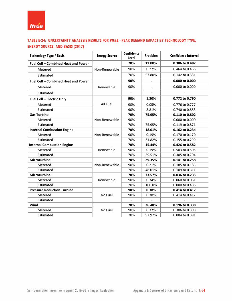
Self-Generation Incentive Program 2016-2017 Impact Evaluation Appendix E: Sources of Uncertainty and Results|E-34
TABLE E-24: UNCERTAINTY ANALYSIS RESULTS FOR PG&E - PEAK DEMAND IMPACT BY TECHNOLOGY TYPE, ENERGY SOURCE, AND BASIS (2017)
Technology Type / Basis Energy Source Confidence Level Precision Confidence Interval
Fuel Cell – Combined Heat and Power Non-Renewable
70% 11.00% 0.386 to 0.482
Metered 90% 0.27% 0.464 to 0.466
Estimated 70% 57.80% 0.142 to 0.531
Fuel Cell – Combined Heat and Power Renewable
90% . 0.000 to 0.000
Metered 90% . 0.000 to 0.000
Estimated - - -
Fuel Cell – Electric Only All Fuel
90% 1.20% 0.772 to 0.790
Metered 90% 0.05% 0.776 to 0.777 Estimated 90% 8.81% 0.740 to 0.883
Gas Turbine Non-Renewable
70% 75.95% 0.110 to 0.802 Metered 90% . 0.000 to 0.000 Estimated 70% 75.95% 0.119 to 0.871
Internal Combustion Engine Non-Renewable
70% 18.01% 0.162 to 0.234 Metered 90% 0.19% 0.170 to 0.170 Estimated 70% 31.82% 0.155 to 0.299
Internal Combustion Engine Renewable
70% 15.44% 0.426 to 0.582 Metered 90% 0.19% 0.503 to 0.505 Estimated 70% 39.51% 0.305 to 0.704
Microturbine Non-Renewable
70% 29.35% 0.141 to 0.258 Metered 90% 0.21% 0.185 to 0.185 Estimated 70% 48.01% 0.109 to 0.311
Microturbine Renewable
70% 73.57% 0.036 to 0.235 Metered 90% 0.34% 0.060 to 0.061 Estimated 70% 100.0% 0.000 to 0.486
Pressure Reduction Turbine No Fuel
90% 0.38% 0.414 to 0.417 Metered 90% 0.38% 0.414 to 0.417 Estimated - - -
Wind No Fuel
70% 26.48% 0.196 to 0.338 Metered 90% 0.32% 0.306 to 0.308 Estimated 70% 97.97% 0.004 to 0.391

Self-Generation Incentive Program 2016-2017 Impact Evaluation Appendix E: Sources of Uncertainty and Results|E-35
TABLE E-25: UNCERTAINTY ANALYSIS RESULTS FOR SCE - PEAK DEMAND IMPACT BY TECHNOLOGY TYPE, ENERGY SOURCE, AND BASIS (2017)
Technology Type / Basis Energy Source Confidence Level Precision Confidence Interval
Fuel Cell – Combined Heat and Power Non-Renewable
70% 7.50% 0.653 to 0.759
Metered 90% 0.27% 0.693 to 0.697
Estimated 70% 32.78% 0.500 to 0.988
Fuel Cell – Combined Heat and Power Renewable
70% 0.00% 0.300 to 0.300
Metered 90% . 0.000 to 0.000
Estimated 70% 0.00% 0.733 to 0.733
Fuel Cell – Electric Only All Fuel
90% 2.11% 0.818 to 0.853
Metered 90% 0.06% 0.843 to 0.844 Estimated 90% 8.83% 0.741 to 0.884
Gas Turbine Non-Renewable
70% 22.74% 0.104 to 0.165 Metered 90% 0.27% 0.089 to 0.090 Estimated 70% 39.41% 0.128 to 0.295
Internal Combustion Engine Non-Renewable
70% 12.13% 0.369 to 0.471 Metered 90% 0.24% 0.406 to 0.408 Estimated 70% 66.20% 0.166 to 0.817
Internal Combustion Engine Renewable
70% 48.39% 0.063 to 0.180 Metered 90% 0.40% 0.100 to 0.101 Estimated 70% 100.0% 0.000 to 0.312
Microturbine Non-Renewable
70% 100.0% 0.000 to 0.177 Metered 90% . 0.000 to 0.000 Estimated 70% 100.0% 0.000 to 0.640
Microturbine Renewable
90% 0.45% 0.477 to 0.481 Metered 90% 0.45% 0.477 to 0.481 Estimated 70% 7.50% 0.653 to 0.759
Pressure Reduction Turbine No Fuel
90% 0.27% 0.693 to 0.697 Metered 70% 32.78% 0.500 to 0.988 Estimated - - -
Wind No Fuel
70% 52.30% 0.045 to 0.145 Metered 90% 0.45% 0.044 to 0.044 Estimated 70% 79.82% 0.051 to 0.458

Self-Generation Incentive Program 2016-2017 Impact Evaluation Appendix E: Sources of Uncertainty and Results|E-36
TABLE E-26: UNCERTAINTY ANALYSIS RESULTS FOR SCG - PEAK DEMAND IMPACT BY TECHNOLOGY TYPE, ENERGY SOURCE, AND BASIS (2017)
Technology Type / Basis Energy Source Confidence Level Precision Confidence Interval
Fuel Cell – Combined Heat and Power Non-Renewable
70% 42.93% 0.231 to 0.579
Metered 90% 0.45% 0.562 to 0.567
Estimated 70% 96.21% 0.011 to 0.589
Fuel Cell – Combined Heat and Power Renewable
90% 0.45% 0.184 to 0.186
Metered 90% 0.45% 0.184 to 0.186
Estimated - - -
Fuel Cell – Electric Only All Fuel
90% 2.11% 0.828 to 0.864
Metered 90% 0.10% 0.856 to 0.857 Estimated 70% 6.44% 0.770 to 0.876
Gas Turbine Non-Renewable
70% 13.90% 0.669 to 0.885 Metered 90% 0.29% 0.872 to 0.877 Estimated 70% 39.44% 0.391 to 0.900
Internal Combustion Engine Non-Renewable
70% 10.94% 0.190 to 0.236 Metered 90% 0.18% 0.206 to 0.207 Estimated 70% 29.65% 0.159 to 0.292
Internal Combustion Engine Renewable
70% 31.78% 0.355 to 0.685 Metered 90% 0.45% 0.554 to 0.559 Estimated 70% 55.59% 0.220 to 0.772
Microturbine Non-Renewable
70% 18.92% 0.221 to 0.324 Metered 90% 0.25% 0.293 to 0.294 Estimated 70% 79.64% 0.045 to 0.397
Microturbine Renewable
90% 0.45% 0.743 to 0.750 Metered 90% 0.45% 0.743 to 0.750 Estimated - - -
Pressure Reduction Turbine No Fuel
- - - Metered - - - Estimated - - -
Wind No Fuel
- - - Metered - - - Estimated - - -