Embed Size (px)
Citation preview
2015 Washington Metropolitan Area Water Supply Study
Demand and Resource Availability
Forecast for the Year 2040 Prepared by S.N. Ahmed, K.R. Bencala, and C.L. Schultz
August 2015 ICPRB Report No. 15-4
The Section for Cooperative Water Supply Operations on the Potomac
Interstate Commission on the Potomac River Basin
30 West Gude Drive, Suite 450 · Rockville, Maryland 20850


2015 Washington Metropolitan Area Water Supply Study:
Demand and Resource Availability Forecast for the Year 2040
Prepared by S.N. Ahmed, K.R. Bencala, and C.L. Schultz
August 2015
ICPRB Report No. 15-4
Copies of this report are available at the ICPRB website, at www.PotomacRiver.org, under “Publications.” To receive printed copies of this report, please write to ICPRB at 30 West Gude Drive, Suite 450, Rockville, MD 20850; or call 301-984-1908.


2015 Washington Metropolitan Area Water Supply Study
Table of Contents
Acknowledgements .................................................................................................................................... viii
Disclaimer .................................................................................................................................................. viii
List of Abbreviations ................................................................................................................................... ix
Executive Summary ..................................................................................................................................... xi
Recent & Forecasted Water Use .............................................................................................................. xi
Upstream Consumptive Demand ........................................................................................................... xiii
Ability of Current System to Meet Forecasted Demands ...................................................................... xiv
System Performance under Repeat of Historical Drought Conditions ............................................... xv
System Performance under Climate Change....................................................................................... xv
Recommendations .................................................................................................................................. xvi
1 Study Objective & Background ......................................................................................................... 1-1
Objective .................................................................................................................................... 1-1
Introduction ................................................................................................................................ 1-2
Water Suppliers .......................................................................................................................... 1-4
History of Cooperation............................................................................................................... 1-4
2 Overview of the Washington Metropolitan Area Water Supply System ........................................... 2-1
System Demands ........................................................................................................................ 2-1
Water Service Areas ........................................................................................................... 2-1
Historical Water Production Trends................................................................................... 2-2
System Resources ...................................................................................................................... 2-4
Potomac River .................................................................................................................... 2-4
Shared Reservoirs .............................................................................................................. 2-4
Additional Resources ......................................................................................................... 2-5
3 Annual Demand Forecast ................................................................................................................... 3-1
Introduction ................................................................................................................................ 3-1
Method for Determining Past Unit Use Rates............................................................................ 3-1
Utility Billing Data............................................................................................................. 3-2
Current & Past Demographic Information ......................................................................... 3-2
Past Unit Use Rates .................................................................................................................... 3-4
Unit Use Trends ................................................................................................................. 3-6
i
2015 Washington Metropolitan Area Water Supply Study
Method for Forecasting Unit Use Rates ..................................................................................... 3-9
Selecting Unit Use Rate for Beginning of Demand Forecast Period ............................... 3-10
Potential Changes in Customer Demand.......................................................................... 3-10
Unit Use Forecast ..................................................................................................................... 3-11
Method for Developing the Annual Demand Forecast ............................................................ 3-13
Demographic Forecast ..................................................................................................... 3-13
Estimate of Unmetered Water Use ................................................................................... 3-18
Annual Demand Forecast ......................................................................................................... 3-19
Comparison of Annual Demand Forecast with Previous Estimates ........................................ 3-21
4 Modeling Daily Variations in Water Demand ................................................................................... 4-1
Data ............................................................................................................................................ 4-2
Removing the Long-term Time Trends ..................................................................................... 4-3
Monthly Mean Production ......................................................................................................... 4-6
Regression Models ..................................................................................................................... 4-9
ARIMA Model ......................................................................................................................... 4-13
Model Demonstration .............................................................................................................. 4-15
Effects of Water Use Restrictions ............................................................................................ 4-17
5 Modeling System Resources & Operations in PRRISM .................................................................... 5-1
Potomac River Flow .................................................................................................................. 5-1
Potomac Flow Recommendations ...................................................................................... 5-3
Reservoir Operations ................................................................................................................. 5-4
North Branch Reservoirs .................................................................................................... 5-4
Use of the Little Seneca, Occoquan, & Patuxent Reservoirs ............................................. 5-7
Effects of Sedimentation on Reservoir Storage ....................................................................... 5-11
Occoquan Reservoir ......................................................................................................... 5-12
Patuxent Reservoirs.......................................................................................................... 5-12
Little Seneca Reservoir .................................................................................................... 5-13
Jennings Randolph Reservoir ........................................................................................... 5-13
Treated Wastewater Return Flows ........................................................................................... 5-15
Production Losses .................................................................................................................... 5-17
Loudoun Water Quarry & Water Treatment Plant ................................................................... 5-19
6 Upstream Consumptive Demand ....................................................................................................... 6-1
Current Upstream Consumptive Use by Use Type .................................................................... 6-1
ii
2015 Washington Metropolitan Area Water Supply Study
Consumptive Demand Estimates for Potomac River Basin Public Water Suppliers ................. 6-3
Forecasts of Upstream Consumptive Use .................................................................................. 6-8
7 Climate Change .................................................................................................................................. 7-1
Approach .................................................................................................................................... 7-2
Potential Changes in Stream Flow ............................................................................................. 7-2
Method Verification ................................................................................................................... 7-4
Projected Changes in Temperature & Precipitation ................................................................... 7-6
Climate Response Function ....................................................................................................... 7-8
8 Results ................................................................................................................................................ 8-1
Model Run Overview & Measures of Performance (Metrics) ................................................... 8-1
Baseline 2035 & 2040 Scenarios ............................................................................................... 8-3
Minimum Reservoir Storage Levels .................................................................................. 8-5
Water Use Restrictions ....................................................................................................... 8-5
Potomac River Shortfalls ................................................................................................... 8-5
Patuxent Shortfalls & Partial Shutdowns ........................................................................... 8-5
Sensitivity of System Performance to Upstream Consumptive Use .......................................... 8-6
Sensitivity of System Performance to Climate Change ............................................................. 8-9
PRRISM Climate Change Results ..................................................................................... 8-9
Future Use of Climate Change Sensitivity Results .......................................................... 8-14
9 Summary & Conclusions ................................................................................................................... 9-1
10 Literature Cited ............................................................................................................................ 10-1
iii

2015 Washington Metropolitan Area Water Supply Study
Table of Appendices Appendix A – Production Data
Appendix B – Calculating the Annual Demand Forecast
Appendix C – Stationarity of Monthly Production Factors
Appendix D – Upstream Consumptive Use
Appendix E – Climate Change Results
Appendix F – PRRISM Input Parameters
iv
2015 Washington Metropolitan Area Water Supply Study
Table of Tables Table 3-1: Unit use values by water supplier (gpd). .................................................................................. 3-5 Table 3-2: Unit use factors calculated in past and current studies (gpd). .................................................. 3-7 Table 3-3: Summary of estimated effects of the Energy Policy Act of 1992 on WMA household water use in 2015 and 2040 (gpd). ........................................................................................................................... 3-11 Table 3-4: Unit use forecast by supplier (gpd)......................................................................................... 3-12 Table 3-5: Projected MWCOG Round 8.3 figures for households, employees, and population by supplier. ................................................................................................................................................................. 3-16 Table 3-6: Predicted demographic change between 2015 and 2040 by supplier. .................................... 3-17 Table 3-7: Comparison of Round 7.2 and Round 8.3 demographics for 2010. ....................................... 3-17 Table 3-8: Difference between Round 8.3 and Round 7.2 demographics for 2010. ................................ 3-17 Table 3-9: Forecasted dwelling unit ratios for each jurisdiction. ............................................................. 3-18 Table 3-10: Unmetered water use assumption for each supplier. ............................................................ 3-19 Table 3-11: Forecast of average annual water demand by supplier, 2015-2040 (MGD). ........................ 3-20 Table 3-12: Change in average annual demand by water use category and supplier, 2015-2040 (MGD). . 3-21 Table 4-1: Goodness-of-fit statistics for long-term time trend options. ..................................................... 4-5 Table 4-2: Empirical coefficients for the linear-quadratic composite model for long-term trend in production for Equation (4-1a) and Equation (4-1b). ................................................................................ 4-6 Table 4-3: Comparison of the 2010 and 2015 ICPRB studies’ long-term stationary means (MGD). ....... 4-6 Table 4-4: Production factors and monthly means by supplier. ................................................................. 4-7 Table 4-5: Spring (March, April, May) regression coefficients for Equation (4-3). ................................ 4-10 Table 4-6: Summer (June, July, August) regression coefficients for Equation (4-3). ............................. 4-11 Table 4-7: Fall (September, October, November) regression coefficients for Equation (4-3). ............... 4-12 Table 4-8: Summer ARIMA(2,0,1) model for the four suppliers. ........................................................... 4-14 Table 4-9: Comparison of statistics for total system demand time series for the period, 2005-2013. ..... 4-16 Table 4-10: Demand reduction percentages assumed for restrictions in model runs. .............................. 4-18 Table 5-1: Town of Westernport withdrawal thresholds for the increased withdrawal amount of 2.2 MGD for industrial use. ....................................................................................................................................... 5-7 Table 5-2: Statistics for low-flow model errors at Little Falls dam (MGD). ............................................. 5-9 Table 5-3: Percent of total demand estimated for each Fairfax Water service area (Gregory Prelewicz, personal communication, January 13, 2015). .......................................................................................... 5-11 Table 5-4: Effects of sedimentation on reservoir storage capacities. ....................................................... 5-12 Table 5-5: Updated estimates of Jennings Randolph Reservoir sedimentation rate and capacity.1 ......... 5-15 Table 5-6: Projected treated wastewater return flows (MGD) from the Seneca, Damascus, Broad Run, and UOSA plants to the Potomac River and Occoquan Reservoir. ................................................................ 5-16 Table 5-7: Production factors (MGD) for treated wastewater return flows for Seneca, Damascus, Broad Run, and UOSA plants. ............................................................................................................................ 5-17 Table 5-8: Assumed production losses for CO-OP system water treatment plants used in PRRISM. .... 5-18 Table 6-1: Current estimated total withdrawals and consumptive use (CU) in the upper Potomac River basin, upstream of the WMA supplier intakes (MGD). ............................................................................. 6-4 Table 6-2: Consumptive use coefficients used in the current study (percent). .......................................... 6-6
v

2015 Washington Metropolitan Area Water Supply Study
Table 6-3: Comparison of monthly PWS consumptive use coefficients from the study by Shaffer (2009), compared with coefficients computed for Potomac basin suppliers (percent). .......................................... 6-8 Table 6-4: Estimates of monthly upstream consumptive use (MGD) in 2010 and growth rates (MGD/yr). ................................................................................................................................................................. 6-10 Table 7-1: Percent change in stream flow associated with the 18 climate change scenarios. .................... 7-4 Table 7-2: Statistics for the linear regression analyses on the two minimum storage projections. ............ 7-6 Table 7-3: Two-sided hypothesis tests comparing the slopes and intercepts from Part 2 of the 2010 demand study and from the verification test. ............................................................................................. 7-6 Table 7-4: Percent changes in average summer flow at Little Falls dam. ................................................. 7-9 Table 7-5: Percent changes in average “other month” flow at Little Falls dam. ..................................... 7-10 Table 8-1: PRRISM results for the 2035 and 2040 baseline scenarios.1 .................................................... 8-4 Table 8-2: PRRISM results for alternative upstream consumptive use (CU) growth rates - 2035 demands.1
................................................................................................................................................................... 8-7 Table 8-3: PRRISM results for alternative upstream consumptive use (CU) growth rates - 2040 demands.1
................................................................................................................................................................... 8-8 Table 8-4: Response of minimum combined system storage (BG) to changes in stream flow - 2040 demands. .................................................................................................................................................. 8-10 Table 8-5: Response of minimum reservoir storage (BG) to changes in stream flow - 2040 demands. .. 8-10 Table 8-6: Response of percentage of years with restrictions to changes in stream flow - 2040 demands. 8-11 Table 8-7: Response of Potomac River flow (MGD) to changes in stream flow - 2040 demands. ......... 8-11 Table 8-8: Response of other performance metrics to percent changes in stream flow - 2040 demands.8-12
vi

2015 Washington Metropolitan Area Water Supply Study
Table of Figures Figure 1-1: WMA water supply resources and areas served by suppliers. ................................................ 1-2 Figure 2-1: Schematic of the Washington metropolitan area’s current and anticipated water sources and suppliers. .................................................................................................................................................... 2-2 Figure 2-2: Historical WSSC, Aqueduct, and Fairfax Water annual production, and combined total annual, summer, winter (by water year), and annual peak-day production. .............................................. 2-3 Figure 3-1: Components of annual demand forecast. ................................................................................ 3-1 Figure 3-2: Areas served by water suppliers in the WMA in 2013. (Note that Vienna became a wholesale customer of Fairfax Water in 2013. Figure 3-4 reflects this and additional changes that occurred in 2014.) ................................................................................................................................................................... 3-3 Figure 3-3: Unit use factors for the three major WMA suppliers for 1990-2013. ..................................... 3-8 Figure 3-4: Areas served by suppliers in the WMA in 2014 and beyond. ............................................... 3-14 Figure 3-5: Comparison of the current study’s WMA annual average demand forecasts with forecasts from earlier studies. ................................................................................................................................. 3-22 Figure 4-1: Production data (gray points) fitted to a linear-quadratic model (black line) with a break point (red point) in the beginning of 2008. ......................................................................................................... 4-4 Figure 4-2: Loudoun Water purchased data (gray points) fitted to a linear-quadratic model (black line) with a break point (red point) in the beginning of 2008. ........................................................................... 4-5 Figure 4-3: Daily production data detrended and compared to the monthly disaggregation of the long-term stationary mean. ......................................................................................................................................... 4-8 Figure 4-4: Daily Loudoun Water purchased data detrended and compared to the monthly disaggregation of the long-term stationary mean. .............................................................................................................. 4-9 Figure 4-5: Regression model results compared with detrended actual data for Fairfax Water, WSSC, Aqueduct, and Loudoun Water. ............................................................................................................... 4-13 Figure 4-6: Total system demand (including Loudoun Water) for the 2002 dry year. ............................ 4-15 Figure 4-7: Total system demand (including Loudoun Water) for the 2010 dry year. ............................ 4-16 Figure 5-1: Adjusted daily flow at Little Falls dam in 2002, daily adjusted flow percentiles for 1930-2013 data, and drought year (2002) demands plus flow-by. ............................................................................... 5-2 Figure 5-2: Comparing the forecast and actual data for historical Little Falls flows from the drought of 1930. .......................................................................................................................................................... 5-9 Figure 5-3: Comparing the forecast and actual data for historical Little Falls flows from the drought of 1966. ........................................................................................................................................................ 5-10 Figure 5-4: Estimated conservation pool storage capacity in Jennings Randolph Reservoir. ................. 5-15 Figure 6-1: Summertime (June, July, August) upstream consumptive use by water use type, excluding the Mount Storm power plant. ......................................................................................................................... 6-5 Figure 6-2: Estimated total PWS withdrawals upstream of WMA intakes. ............................................... 6-7 Figure 7-1: Projections of minimum combined Jennings Randolph water supply storage and Little Seneca Reservoir storage, given 2040 demands. ................................................................................................... 7-5 Figure 7-2: Projected change in temperature and precipitation for the Potomac River basin.................... 7-7 Figure 7-3: Other month flow percent change versus summer percent change. ........................................ 7-9 Figure 8-1: Predicted Potomac reserve versus percent change in summer basin-wide stream flow for a severe drought (percent changes applied to 1930 flows), given 2040 demands. ..................................... 8-13
vii
2015 Washington Metropolitan Area Water Supply Study
Acknowledgements Funds were provided for this report by the three major Washington, D.C., metropolitan area water suppliers: the Washington Suburban Sanitary Commission (WSSC); the Washington Aqueduct Division of the U.S. Army Corps of Engineers; and Fairfax Water.
This report would not have been possible without the many people who generously provided us with data and information. We thank the following individuals, as well as those whom we may have neglected to mention: Greg Prelewicz and Traci Kammer-Goldberg of Fairfax Water; Fatima Khaja of Fairfax County; Eric Forman of the City of Fairfax; Anne Spiesman and Alex Gorzalski of Washington Aqueduct; Nick Gardner and Kimberly Six of WSSC; Dave Hundelt of the Arlington County; Charles Sweeney and Lauren Preston of DC Water; Thomas Lipinski of Loudoun Water; Jill Kaneff of Loudoun County; David Guerra of Prince William County Service Authority; Frank Hunt, David McGettigan, and Bill Vaughan of Prince William County; Gary Fuller of the City of Falls Church; Ilene Lish and Manisha Tewari of the City of Rockville; Andrew Barnes and Dana Heiberg of the Town of Herndon; Marion Serfass of the Town of Vienna; Pat Mann of the City of Alexandria; Robert Ruiz of Montgomery County; Ted Kowaluk of the Maryland National Capital Park and Planning Commission.
We would especially like to thank Greg Prelewicz of Fairfax Water, Nick Gardner of WSSC, and Anne Spiesman of Washington Aqueduct for their advice and guidance and for taking the time to answer our many questions, and Roland Steiner of WSSC for his careful review of and comments on the report.
Disclaimer This report was prepared by the Interstate Commission on the Potomac River Basin, Section for Cooperative Water Supply Operations on the Potomac. The opinions expressed are those of the authors and should not be construed as representing the opinions or policies of the United States or any of its agencies, the several states, the Commissioners of the Interstate Commission on the Potomac River Basin, or the water suppliers.
viii

2015 Washington Metropolitan Area Water Supply Study
List of Abbreviations °C Degrees Celsius
°F Degrees Fahrenheit
AQU Aquaculture
ARIMA Autoregressive integrated moving average
BG Billion gallons
BRWRF Broad Run Water Reclamation Facility
CO-OP ICPRB’s Section for Cooperative Water Supply Operations on the Potomac
COM Self-supplied commercial
CU Consumptive use
DC Water District of Columbia Water and Sewer Authority
FW or Fairfax Water Fairfax County Water Authority
GCM General circulation model
gpd Gallons per day
HSPF Hydrologic Simulation Program – FORTRAN
ICPRB Interstate Commission on the Potomac River Basin
IND Self-supplied industry
IRRA Agricultural irrigation
IRRG Golf course irrigation
LFAA Low Flow Allocation Agreement
LIV Livestock
LW Loudoun Water
MAE Mean absolute error
ME Mean error
MSE Mean square error
MG Million gallons
MGD Million gallons per day
MGS Maryland Geological Survey
MIN Mining
MSL Mean sea level
MWCOG Metropolitan Washington Council of Governments
PP Thermoelectric power generation
PRRISM Potomac Reservoir and River Simulation Model
PWS Public water supply
ix

2015 Washington Metropolitan Area Water Supply Study
R2 Coefficient of determination
RMSE Root mean square error
SE Standard error
SD Standard deviation
SSD Self-supplied domestic use
UPRC Upper Potomac River Commission
USACE U.S. Army Corps of Engineers
USGS U.S. Geological Survey
WMA Washington, D.C., metropolitan area
WSCA Water Supply Coordination Agreement
WSSC Washington Suburban Sanitary Commission
WWTP Wastewater treatment plant
x

2015 Washington Metropolitan Area Water Supply Study
Executive Summary
This study provides forecasts of Washington, D.C., metropolitan area water demands through the year 2040 and assesses the ability of current system resources to meet those demands. The Potomac River is the primary water supply source for residents, businesses, and government facilities located in the Washington, D.C., metropolitan area (WMA). This study defines the WMA as the District of Columbia and the District’s Virginia and Maryland suburbs, including the City of Rockville. The main water suppliers for the WMA – the U.S. Army Corps of Engineers Washington Aqueduct Division (Aqueduct), Fairfax County Water Authority (Fairfax Water), and Washington Suburban Sanitary Commission (WSSC) (referred to in this report as the “CO-OP suppliers”) – have a long history of cooperation. This cooperative approach was formalized in a set of agreements signed in the late 1970s and early 1980s. These agreements include the Low Flow Allocation Agreement (LFAA), which allocates the amount of water each supplier can withdraw from the Potomac River in the event that total flow is not sufficient to meet all needs; the Water Supply Coordination Agreement (WSCA), which provides for coordinated operations during periods of low flow and regular planning studies; and multiple joint funding agreements covering shared storage in reservoirs located upstream of the WMA. During periods when Potomac River flows are low, these suppliers coordinate their operations with the assistance of ICPRB’s Section for Cooperative Water Supply Operations on the Potomac (CO-OP) in order to optimize use of available resources and maintain adequate flow downstream of their Potomac intakes to protect aquatic habitats.
Recent & Forecasted Water Use
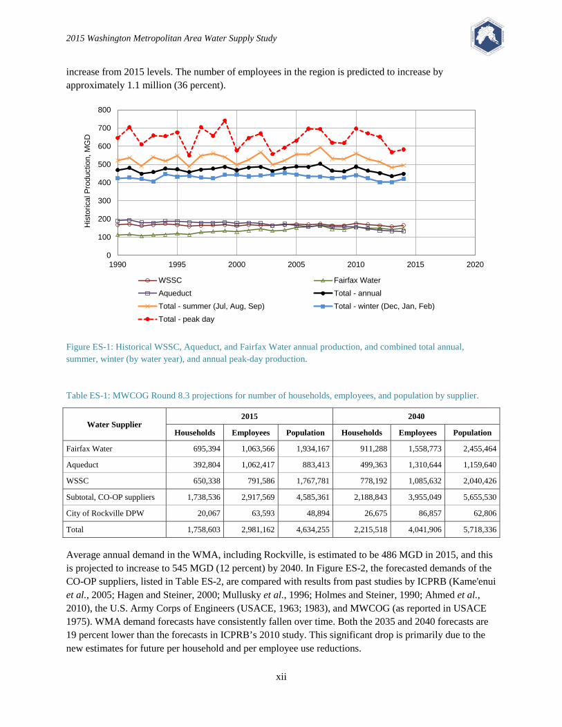
Water use in the WMA has held remarkably steady during the past two decades, averaging 466 million gallons per day (MGD) in recent years (2009-2013). Figure ES-1 shows total annual, summer, and winter water production by the CO-OP suppliers, as well as annual peak-day production, from 1990-2013. Though the WMA population rose 18 percent from 1990-2015, from 3.9 to 4.6 million people, its water demands have essentially remained constant over that period due to falling per household and per employee use. This decline in unit use is consistent with trends seen throughout the United States.
To improve forecasts of future household use this study uses a new model which accounts for future reductions in indoor use attributed to the U.S. Environmental Protection Agency’s WaterSense program and the U.S. Department of Energy’s Energy Star program, as well as reductions from the Energy Policy Act of 1992. The model estimates a reduction in indoor household use of 25.3 gallons per day between 2015 and 2040.
Forecasts of average annual water demand were developed by combining recent water use information derived from billing data provided by the suppliers and their wholesale customers, information on the current and future extent of the areas supplied, and the most recent demographic forecasts (Round 8.3) from the Metropolitan Washington Council of Governments (MWCOG). Forecasts were also made for the City of Rockville, which is part of the WMA but independently produces and delivers water to its customers. Water use data was disaggregated into three categories for forecasting purposes: single family households, multi-family households (apartments), and employees (including commercial, industrial, and institutional use). MWCOG projects that population in the WMA in 2040 will be 5.7 million, a 23 percent
xi
2015 Washington Metropolitan Area Water Supply Study
increase from 2015 levels. The number of employees in the region is predicted to increase by approximately 1.1 million (36 percent).
Figure ES-1: Historical WSSC, Aqueduct, and Fairfax Water annual production, and combined total annual, summer, winter (by water year), and annual peak-day production.
Table ES-1: MWCOG Round 8.3 projections for number of households, employees, and population by supplier.
Water Supplier 2015 2040
Households Employees Population Households Employees Population
Fairfax Water 695,394 1,063,566 1,934,167 911,288 1,558,773 2,455,464
Aqueduct 392,804 1,062,417 883,413 499,363 1,310,644 1,159,640
WSSC 650,338 791,586 1,767,781 778,192 1,085,632 2,040,426
Subtotal, CO-OP suppliers 1,738,536 2,917,569 4,585,361 2,188,843 3,955,049 5,655,530
City of Rockville DPW 20,067 63,593 48,894 26,675 86,857 62,806
Total 1,758,603 2,981,162 4,634,255 2,215,518 4,041,906 5,718,336
Average annual demand in the WMA, including Rockville, is estimated to be 486 MGD in 2015, and this is projected to increase to 545 MGD (12 percent) by 2040. In Figure ES-2, the forecasted demands of the CO-OP suppliers, listed in Table ES-2, are compared with results from past studies by ICPRB (Kame'enui et al., 2005; Hagen and Steiner, 2000; Mullusky et al., 1996; Holmes and Steiner, 1990; Ahmed et al., 2010), the U.S. Army Corps of Engineers (USACE, 1963; 1983), and MWCOG (as reported in USACE 1975). WMA demand forecasts have consistently fallen over time. Both the 2035 and 2040 forecasts are 19 percent lower than the forecasts in ICPRB’s 2010 study. This significant drop is primarily due to the new estimates for future per household and per employee use reductions.
0
100
200
300
400
500
600
700
800
1990 1995 2000 2005 2010 2015 2020
His
toric
al P
rodu
ctio
n, M
GD
WSSC Fairfax Water
Aqueduct Total - annual
Total - summer (Jul, Aug, Sep) Total - winter (Dec, Jan, Feb)
Total - peak day
xii

2015 Washington Metropolitan Area Water Supply Study
Figure ES-2: Comparison of Washington metropolitan area water supplier average annual demand.
Table ES-2: Forecast of average annual water demand for the WMA from 2015-2040 (MGD).
Water Supplier 2015 2020 2025 2030 2035 2040
Fairfax Water 188.5 192.0 200.5 209.4 214.5 222.2
Aqueduct 125.4 126.0 129.4 133.4 134.6 138.1
WSSC 167.4 164.6 166.9 171.4 174.1 179.3
Subtotal, CO-OP suppliers 481.3 482.7 496.8 514.2 523.2 539.6
City of Rockville DPW 4.9 4.9 5.0 5.3 5.4 5.7
Total 486.3 487.6 501.8 519.5 528.6 545.3
Upstream Consumptive Demand
Communities, farms, and industries located upstream of the WMA withdraw water from the Potomac River, its tributaries, and its groundwater aquifers. These upstream users impact the amount of water available to meet downstream needs. Much of the water withdrawn upstream is returned to watershed streams, for example, as water discharged by wastewater treatment plants. However, a portion is not returned due to evaporation, transpiration, incorporation into products, consumption by humans or
0.0
1.0
2.0
3.0
4.0
5.0
6.0
200
300
400
500
600
700
800
900
1000
1960 1970 1980 1990 2000 2010 2020 2030 2040
Popu
latio
n (M
illion
s)
Dem
and
(MG
D)
MWCOG, 1975
Population
USACE, 1983
ICPRB, 1990
ICPRB, 1995
ICPRB, 2000
ICPRB, 2010 (high)
ICPRB, 2010
ICPRB, 2005ICPRB, 2015
USACE, 1963
Actual Water Demands
xiii

2015 Washington Metropolitan Area Water Supply Study
livestock, diversion to another basin, or other processes. The portion of water withdrawn that is removed and not returned to be available for downstream use is termed “consumptive demand,” or equivalently in this study, “consumptive use.” The forecasts of upstream consumptive demand and its impact on WMA supplies are accounted for in the water availability analysis.
This study contains updated estimates of consumptive use upstream of the WMA suppliers’ Potomac River intakes. These were derived using ICPRB’s new database of Potomac basin water withdrawals and consumptive use, described in Ducnuigeen et al. (2015). Summertime upstream consumptive demand has the greatest impact on the WMA water supply system, since WMA demands are at their highest in the summer and flow in the Potomac River tends to be falling. The water use categories considered in this study are: aquaculture (AQU), self-supplied commercial (COM), self-supplied industry (IND), golf course irrigation (IRRG), mining (MIN), thermoelectric power generation (PP), public water supply (PWS), agricultural irrigation (IRRA), livestock (LIV), and self-supplied domestic use (SSD). A breakdown of average summertime (June, July, August) upstream consumptive use by use type is shown in Figure ES-3.1 Public water supply accounts for the greatest forecasted growth in summer consumptive use. Average total upstream consumptive use in the summer months (June, July, August) is estimated to be 111 MGD in 2015 and is projected to grow to 141 MGD in 2040, an increase of 27 percent.
Figure ES-3: Summertime (June, July, August) upstream consumptive use by water use type.
Ability of Current System to Meet Forecasted Demands
The aim of this study is to assess the ability of current water supply resources to meet projected WMA demands over a 25-year forecast horizon, both under conditions similar to historical droughts and taking into account potential changes in stream flow due to climate change. This evaluation was conducted using
1 This excludes West Virginia’s Mount Storm power plant, whose withdrawals are mitigated by releases from downstream reservoirs.
Aquaculture2% Commercial
1%
Ag irrigation20%
Golf irrigation7%
Livestock11%
Mining5%Power
9%
Industry19%
Public supply19%
Residential wells7%
xiv

2015 Washington Metropolitan Area Water Supply Study
ICPRB’s Potomac Reservoir and River Simulation Model (PRRISM). PRRISM simulates on a daily basis the processes that govern WMA water demand and availability, including:
• upstream consumptive demands; • flows in the Potomac River; • inflows, storage, and releases from the system of reservoirs; and • water withdrawals by the WMA suppliers.
PRRISM was used to evaluate how the current system would respond to forecasted water demands under the range of hydrologic conditions that occurred over the historic record, from 1929-2013, and under a range of potential conditions altered by climate change.
System Performance under Repeat of Historical Drought Conditions
Under a repeat of conditions similar to severe historic droughts, assuming no impact from climate change, PRRISM simulations predict that by 2035 the current water supply system will experience considerable stress, with mandatory water use restrictions required in the WMA. By 2040 there is some likelihood that storage in Little Seneca Reservoir will become exhausted. In both 2035 and 2040 there is a small probability that flow in the Potomac River would drop below the minimum environmental flow level of 100 MGD at Little Falls dam, though the predicted flow deficit is less than 1 MGD.
System Performance under Climate Change
To assess the potential impact of climate change on the performance of the current WMA water supply system, a sensitivity test was conducted by applying projected basin-wide percent changes in long-term average seasonal stream flow to the natural historic stream flow records used in PRRISM. The range of stream flow alterations projected for the Potomac basin by 2040 is large, and the corresponding impact on system performance varies dramatically depending on the change in stream flow. Results from this study indicate that in the event of a severe drought with 2040 forecasted demands, the following range of potential impacts on the WMA system could be expected due to long-term changes in average summer (June, July, August) stream flows:
• If summer flows fall by 10 percent or more: the decrease in flows would cause mandatory water use restrictions to occur; over the course of the severe drought, most system reservoirs would be drained and on some days the system would be unable to meet demands and the 100 MGD environmental flow-by at Little Falls.
• If summer flows change by 0 to +10 percent: the moderate increase in flows would not be enough to prevent mandatory water use restrictions from occurring during a severe drought; storage in the Patuxent and Little Seneca reservoirs could be seriously depleted.
• If summer flows rise by 20 percent or more: a substantial increase in flows would increase WMA supplies sufficiently to allow the current WMA system to meet forecasted 2040 demands.
Changes in long-term average stream flow used in the sensitivity test were obtained from climate response functions (Brown et al., 2011). The climate response functions link changes in seasonal basin-wide stream flow to potential changes in temperature and precipitation, and were developed from Chesapeake Bay Program Watershed Model stream flow output for climate change projections from
xv

2015 Washington Metropolitan Area Water Supply Study
ICPRB’s previous climate change study (Ahmed et al., 2013). Table ES- 3 shows climate response function predictions of changes in summer Potomac River flow for a range of changes in average temperature and precipitation. A 10 percent or greater decrease in summer stream flows is indicated by the shaded region of Table ES-3; this change is associated with serious adverse impacts to the WMA system, as discussed above. The climate response functions derived in this study provide water resource managers with information that can assist in the interpretation of new climate projections and research results on long-term hydrological trends as they become available.
Table ES- 3: Percent changes in average summer (June, July, August) Potomac River flow at Little Falls dam as a function of change in temperature and precipitation.
Precipitation Change, Percent
-10.0 -7.5 -5.0 -2.5 0.0 2.5 5.0 7.5 10.0
Tem
pera
ture
Cha
nge,
°F
0.0 -23 -17 -11 -6 0 6 11 17 23
0.5 -24 -19 -13 -8 -2 4 9 15 21
1.0 -26 -21 -15 -9 -4 2 7 13 19
1.5 -28 -23 -17 -11 -6 0 6 11 17
2.0 -30 -24 -19 -13 -8 -2 4 9 15
2.5 -32 -26 -21 -15 -9 -4 2 7 13
3.0 -34 -28 -23 -17 -11 -6 0 6 11
3.5 -36 -30 -24 -19 -13 -8 -2 4 9
4.0 -38 -32 -26 -21 -15 -9 -4 2 7
Recommendations
Recommended actions for consideration, based on the findings of this study, include the following: 1. The region’s water suppliers should continue their efforts to identify and evaluate potential new
water supply storage facilities. CO-OP should conduct an evaluation of the relative benefits to the system of a suite of potential options, including new storage facilities and non-structural changes in operations.
2. CO-OP should continue its development of real-time flow forecast tool, to help reduce flow forecast errors and minimize the probability that Potomac River flows will fall below environmental flow targets during droughts.
3. Support should be identified for further development of ICPRB’s database and model of Potomac basin water withdrawals and consumptive use to provide a sound foundation for basin-wide water supply planning and for the planned basin-wide comprehensive plan.
xvi

2015 Washington Metropolitan Area Water Supply Study
1 Study Objective & Background
Objective
The objective of the 2015 Washington Metropolitan Area Water Supply Study is to aid long-range water resource planning by
a) Forecasting water demands for the Washington, D.C., metropolitan area through the year 2040, taking into account projected demographic and societal changes that may affect future water use.
b) Evaluating the ability of current water supply resources to meet these projected demands, taking into account the potential impact of climate change.
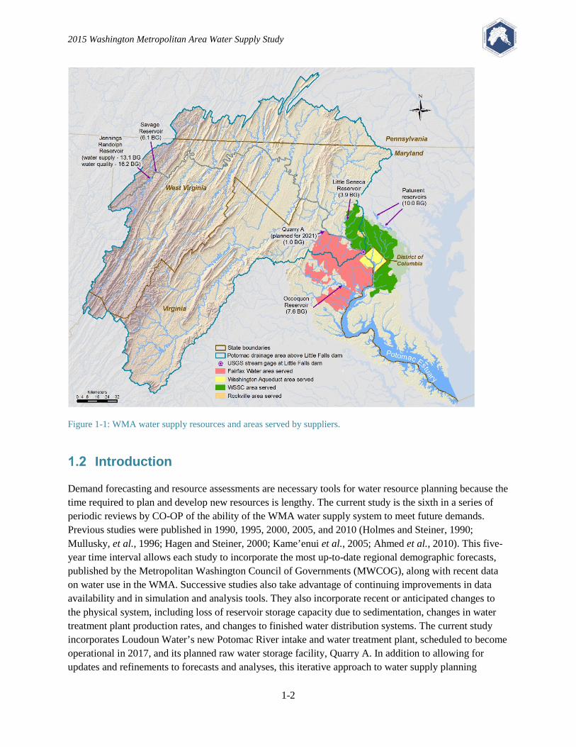
This study has been conducted by the Section for Cooperative Water Supply Operations on the Potomac (CO-OP) of the Interstate Commission on the Potomac River Basin (ICPRB) on behalf of the three major water suppliers (“CO-OP suppliers”): Fairfax County Water Authority (Fairfax Water), the Washington Suburban Sanitary Commission (WSSC), and the Washington Aqueduct (Aqueduct). The Washington, D.C., metropolitan area (WMA) (shown in Figure 1-1) is defined in this study as the District of Columbia and the portions of the Maryland and Virginia suburbs that are supplied water, either directly or indirectly, by the CO-OP suppliers and/or by Loudoun Water. It also includes the City of Rockville. Current water supply resources are defined as the Potomac River upstream of Little Falls dam near Washington, D.C., and the six existing or planned reservoirs depicted in Figure 1-1.
The study satisfies a requirement specified in both the Low Flow Allocation Agreement (LFAA), as amended by Modification 1, signed in 1978 by the United States, the State of Maryland, the Commonwealth of Virginia, the District of Columbia, WSSC, and Fairfax Water; and the Water Supply Coordination Agreement (WSCA), signed in 1982 by the United States, Fairfax Water, WSSC, the District of Columbia, and ICPRB. As stated in the WSCA, it is agreed that “In April 1990 and in April of each fifth year thereafter… the Aqueduct, the Authority, the Commission and the District shall review and evaluate the adequacy of the then available water supplies to meet the water demands in the Washington Metropolitan Area which may then be expected to occur during the succeeding 20-year period.” The specified 20-year period has been extended in the current study to include a 25-year planning horizon since demographic forecasts are currently available through 2040.
1-1
2015 Washington Metropolitan Area Water Supply Study
Figure 1-1: WMA water supply resources and areas served by suppliers.
Introduction
Demand forecasting and resource assessments are necessary tools for water resource planning because the time required to plan and develop new resources is lengthy. The current study is the sixth in a series of periodic reviews by CO-OP of the ability of the WMA water supply system to meet future demands. Previous studies were published in 1990, 1995, 2000, 2005, and 2010 (Holmes and Steiner, 1990; Mullusky, et al., 1996; Hagen and Steiner, 2000; Kame’enui et al., 2005; Ahmed et al., 2010). This five-year time interval allows each study to incorporate the most up-to-date regional demographic forecasts, published by the Metropolitan Washington Council of Governments (MWCOG), along with recent data on water use in the WMA. Successive studies also take advantage of continuing improvements in data availability and in simulation and analysis tools. They also incorporate recent or anticipated changes to the physical system, including loss of reservoir storage capacity due to sedimentation, changes in water treatment plant production rates, and changes to finished water distribution systems. The current study incorporates Loudoun Water’s new Potomac River intake and water treatment plant, scheduled to become operational in 2017, and its planned raw water storage facility, Quarry A. In addition to allowing for updates and refinements to forecasts and analyses, this iterative approach to water supply planning
1-2
2015 Washington Metropolitan Area Water Supply Study
increases the visibility of regional water supply issues and fosters communication between regional stakeholders (Hagen et al., 2005).
The 2015 study largely follows the methodology developed in recent ICPRB studies. It includes two main components: a demand forecast and a resource availability assessment. Forecasts of average annual water demand are developed by combining end-use customer billing data provided by the suppliers, information from suppliers and local planning agencies on the current and future extent of water service areas, and the most recent demographic forecasts from MWCOG. Seasonal and daily variations in demand, dependent on the time of year, day of the week, and meteorological conditions, are simulated using statistical regression and modeling techniques similar to those used by Ahmed et al., 2010; Kame’enui et al., 2005; and Steiner, 1984.
The resource availability assessment is conducted using ICPRB’s Potomac Reservoir and River Simulation Model (PRRISM) to simulate future water demand and availability for the WMA. The current version of PRRISM was developed using the object-oriented programming language ExtendSim™ Version 8 (Imagine That!, Inc.). PRRISM simulates on a daily basis the processes that govern water supply and demand in the system, including
• consumptive demands upstream of the WMA; • flows in the Potomac River; • inflows, storage, and releases from reservoirs; and • withdrawals by WMA suppliers.
The resource analysis evaluates how the WMA’s current system of water supply resources, the Potomac River and the existing or planned storage facilities shown in Figure 1-1, would respond to forecasted water demands under the range of hydrologic conditions that occurred from 1929-2013. It also assesses the vulnerability of the system to changes in stream flow that might occur during a severe, prolonged drought in a basin altered by global climate change. The climate change vulnerability assessment is informed by watershed modeling results obtained in Part 2 of CO-OP’s 2010 water supply forecast (Ahmed et al., 2013, herein referred to as Part 2 of the 2010 demand study).
The 2015 study includes the following updates and refinements: • incorporation of forecasts of monthly consumptive water use upstream of the WMA, derived
from data in ICPRB’s new Potomac River basin monthly withdrawal and consumptive use database, which replace the estimated summer and non-summer values from Steiner et al.(2000);
• a new forecast model for future declines in indoor water use based on reductions due to the U.S. Environmental Protection Agency’s WaterSense program, the U.S. Department of Energy’s Energy Star program, and standards imposed by the Energy Policy Act of 1992;
• improved representation of inefficiencies related to releases from Little Seneca Reservoir and use of Occoquan Reservoir during low-flow periods, due to current limitations in the accuracy of flow forecasts;
• recent changes in the region’s water suppliers, including the incorporation of the City of Fairfax and the City of Falls Church into the Fairfax Water system;
1-3
2015 Washington Metropolitan Area Water Supply Study
• Loudoun Water’s new intake on the Potomac River and Trap Rock Water Treatment Facility, expected to commence operations in 2017, and their use of a retired quarry (Quarry A) as a water storage facility beginning in 2021; and
• inclusion of the Town of Westernport’s additional withdrawal from Savage Reservoir.
Water Suppliers
The Potomac River is the primary water supply source for the WMA. This study represents the operations of the five WMA suppliers, listed below, that withdraw and treat water from the Potomac River (either currently or in the near future):
• Aqueduct, a Division of the U.S. Army Corps of Engineers (USACE), serving the District of Columbia via the District of Columbia Water and Sewer Authority (DC Water) and Arlington County, Virginia, and serving Falls Church, Virginia, via sale of water to Fairfax Water;
• WSSC, serving Montgomery and Prince George’s counties in Maryland, and providing a limited amount of water to Howard and Charles counties, and providing water on an emergency basis to the City of Rockville and to DC Water;
• Fairfax Water, serving most of Fairfax County, Virginia, and certain other Virginia suburbs; • City of Rockville, in Montgomery County, Maryland; and • Loudoun Water, in Loudoun County, Virginia; Loudoun Water currently supplies its customers
with water purchased from Fairfax Water, but in 2017 it will begin supplying a portion of its demand with water withdrawn from the Potomac River and produced by its new water treatment plant.
Collectively, these suppliers obtain approximately three quarters of their water from the Potomac River. The CO-OP suppliers – Aqueduct, WSSC, and Fairfax Water – jointly have rights to use water stored in two upstream reservoirs: Jennings Randolph and Little Seneca. Water in these reservoirs can be released during times of drought to augment natural river flow. In addition, Fairfax Water and WSSC rely, on a daily basis, on water stored in reservoirs which are outside of the drainage area of the fresh water portion of the Potomac River, on the Occoquan River and the Patuxent River, respectively. Loudoun Water’s Quarry A, scheduled for completion in 2021, will provide a portion of its supply during droughts, under conditions specified in its Water Protection Permit.
History of Cooperation
Concern about WMA water supply began in the 1960s. The population of the WMA was expected to grow to five million by 1985 (USACE, 1963), after having grown from 672,000 in 1930 to two million in 1960. During this same time period, drought-induced rationing was viewed as a real threat, as demand was forecasted to exceed the low flow of the largely unregulated (meaning few dams) Potomac River (Potomac Basin Reporter, 1982).
Potential measures for increasing water supply were evaluated during this period. The USACE conducted a study that identified 16 potential dam sites on the Potomac River upstream of Washington, D.C., whose reservoirs could augment supply during low-flow periods (USACE, 1963). There was significant public
1-4
2015 Washington Metropolitan Area Water Supply Study
opposition to many of these sites and only one, Jennings Randolph Reservoir near Bloomington, Maryland, was constructed. Other alternatives that were studied included estuary treatment plants, interconnections in the distribution systems, and inter-basin transfers (Ways, 1993).
The actual WMA population in 1985, approximately 3.1 million people (United States Census Bureau, 2004), was lower than forecasted by the USACE. However, WMA demand levels exceeded the Potomac River’s 1966 low-flow record 41 times during the period between 1971 and 1982 (Ways, 1993). The WMA did not experience water supply shortages during this period only because no serious droughts occurred.
Given the opposition to constructing reservoirs, the suppliers and local governments searched for other solutions. By the late 1970s, researchers at Johns Hopkins University had developed the basis of the cooperative system used today (Palmer et al., 1979; 1982; Sheer, 1977). This research indicated that the management of Jennings Randolph Reservoir, scheduled to be completed soon, in coordination with the existing Occoquan and Patuxent reservoirs, could meet the region’s projected demand and maintain adequate flow in the Potomac River through about 2020. Increased system reliability stems from operating rules which specify that participating suppliers depend more heavily on the free-flowing Potomac River during winter and spring months of low-flow years in order to preserve storage in the Patuxent and Occoquan reservoirs. This strategy is possible because even during droughts, the winter and spring Potomac River flow is more than adequate to meet water supply demand. This operating policy ensures that the Patuxent and Occoquan reservoirs remain available for use during the summer low-flow season and reduces the probability of system failure. Thus, a regional consensus emerged, minimizing the need for new dams or other costly and controversial structural measures.
Following this consensus, key agreements governing this cooperative approach were forged. In 1978, the U.S. Army (representing Aqueduct), Maryland, Virginia, the District of Columbia, Fairfax Water, and WSSC signed the LFAA. The agreement defines how Potomac River water withdrawals will be allocated between the suppliers in the event that the total flow is not sufficient to meet the needs of each supplier. These allocations are set annually, based on winter water use.
On July 22, 1982, eight agreements were signed that established the WMA’s cooperative system of water supply management, which includes shared funding and use of regional resources, coordinated operations during periods of drought, and regular forecasts of future water demands. Fairfax Water, WSSC, the District of Columbia, the USACE (representing Aqueduct), and ICPRB signed the WSCA. This agreement provides for the coordinated use of the major water supply facilities in the region, including those on the Patuxent and Occoquan rivers, as a means of minimizing the potential of triggering the LFAA’s low-flow allocation mechanism. Under the WSCA, the suppliers cooperate by operating as one entity that shares water across the Potomac, Patuxent, and Occoquan basins during low-flow periods.
The CO-OP suppliers jointly pay the capital and operating costs for Little Seneca Reservoir, which was completed in 1985, and for a portion of the water stored in the Jennings Randolph Reservoir, which was completed in 1981. These reservoirs are used during droughts to augment the natural flow of the Potomac River. Together, these sources provide approximately 17 billion gallons (BG) of storage upstream of the WMA Potomac River intakes designated for water supply purposes. The CO-OP suppliers also contribute to the operating costs of Savage River Reservoir.
1-5
2015 Washington Metropolitan Area Water Supply Study
As specified in the WSCA, ICPRB’s CO-OP Section assumes a direct role in managing water supply resources and WMA withdrawals during droughts. The WSCA established an Operations Committee, consisting of representatives from the Aqueduct, Fairfax Water, and WSSC, that is responsible for overseeing CO-OP activities. The agreement assigns to CO-OP the responsibility, in consultation with the suppliers, of directing water supply releases from Jennings Randolph and Little Seneca reservoirs and setting Potomac River withdrawal rates. This portion of the agreement was driven by the realization that coordinated operations would allow each supplier to meet their own demands and collectively meet the demands of the region. This decision to seek a joint solution to potential water supply shortages has made it possible to provide adequate water supply to the WMA in a manner that has been far less expensive than other proposed solutions.
Since the establishment of the CO-OP system in 1982, water supply releases to augment the natural flow of the Potomac River for water supply purposes have been made in only three years. Water supply releases were made from Jennings Randolph and Little Seneca reservoirs during low-flow periods in the summers of 1999 and 2002 and during the fall of 2010. In each of these years, cooperative operations ran smoothly, and the augmented flow of the Potomac provided the required water.
1-6
2015 Washington Metropolitan Area Water Supply Study
2 Overview of the Washington Metropolitan Area Water Supply System
This chapter provides an overview of the WMA water supply system, including the resources which provide water and the entities that withdraw, treat, and distribute the water to area residents, businesses, and institutions. Figure 1-1 shows the areas served by the WMA suppliers, system resources, and the U.S. Geological Survey (USGS) stream gage at Little Falls dam near Washington, D.C. This gage measures flow in the Potomac River downstream of WMA Potomac intakes. CO-OP’s goal during droughts is to operate in a manner that optimizes use of system resources, meets customers’ water demands, and maintains flow in the Potomac River at Little Falls dam above the environmental flow-by of 100 million gallons per day (MGD), equivalent to 155 cubic feet per second (cfs). More detailed descriptions of the system components are given in Chapter 5.
System Demands
The WMA suppliers provide water to approximately 4.6 million people who reside in their combined water service areas (Figure 1-1).
2.1.1 Water Service Areas
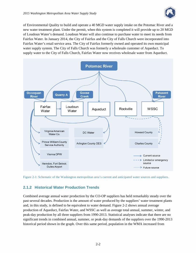
The WMA water suppliers and their water sources are shown in the schematic diagram in Figure 2-1. Four of these water suppliers currently withdraw and treat water from the Potomac River and distribute it directly to homes, businesses, and institutions located in their “retail” service areas, and/or sell treated water to “wholesale” customers. The wholesale customers are water suppliers that own water distribution systems in other areas of the WMA. As discussed in more detail below, a fifth supplier, Loudoun Water, currently purchases all of its water wholesale from Fairfax Water, but in the near future will begin supplying a portion of its demand with water withdrawn and treated via its new intake and water treatment plant on the Potomac River.
Fairfax Water provides water to customers in its retail service area in Fairfax County. It also serves other areas via its wholesale customers: Loudoun Water, Prince William County Service Authority, Virginia American Water Company (providing water to the City of Alexandria and Dale City), Dulles Airport, and the Vienna Department of Public Works (DPW). Aqueduct sells water to wholesale customers that provide water to the District of Columbia and Arlington: the District of Columbia Water and Sewer Authority (DC Water) and Arlington County Department of Environmental Services (DES). Aqueduct also supplies water on a wholesale basis to Fairfax Water for distribution to Fairfax Water’s retail customers in Falls Church, Virginia. WSSC serves Prince George’s and Montgomery counties, provides water on an emergency basis to the City of Rockville, and also provides a limited amount of water to Charles and Howard counties, all in Maryland. Rockville owns and operates its own water supply system which withdraws water from an intake on the Potomac River just downstream of WSSC’s intake.
A number of changes to the supplier service areas have taken place since 2010. In November 2012, Loudoun Water, a wholesale customer of Fairfax Water, obtained a permit from the Virginia Department
2-1
2015 Washington Metropolitan Area Water Supply Study
of Environmental Quality to build and operate a 40 MGD water supply intake on the Potomac River and a new water treatment plant. Under the permit, when this system is completed it will provide up to 20 MGD of Loudoun Water’s demand. Loudoun Water will also continue to purchase water to meet its needs from Fairfax Water. In January 2014, the City of Fairfax and the City of Falls Church were incorporated into Fairfax Water’s retail service area. The City of Fairfax formerly owned and operated its own municipal water supply system. The City of Falls Church was formerly a wholesale customer of Aqueduct. To supply water to the City of Falls Church, Fairfax Water now receives wholesale water from Aqueduct.
Figure 2-1: Schematic of the Washington metropolitan area’s current and anticipated water sources and suppliers.
2.1.2 Historical Water Production Trends
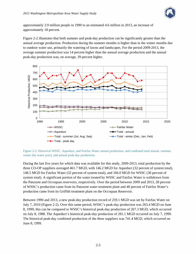
Combined average annual water production by the CO-OP suppliers has held remarkably steady over the past several decades. Production is the amount of water produced by the suppliers’ water treatment plants and, in this study, is defined to be equivalent to water demand. Figure 2-2 shows annual average production of Aqueduct, Fairfax Water, and WSSC as well as average total annual, summer, winter, and peak-day production by all three suppliers from 1990-2013. Statistical analyses indicate that there are no significant trends in combined annual, summer, or peak-day demands of the suppliers over the 1990-2013 historical period shown in the graph. Over this same period, population in the WMA increased from
2-2
2015 Washington Metropolitan Area Water Supply Study
approximately 3.9 million people in 1990 to an estimated 4.6 million in 2013, an increase of approximately 18 percent.
Figure 2-2 illustrates that both summer and peak-day production can be significantly greater than the annual average production. Production during the summer months is higher than in the winter months due to outdoor water use, primarily the watering of lawns and landscapes. For the period 2009-2013, the average summer production was 14 percent higher than the annual average production and the annual peak-day production was, on average, 39 percent higher.
Figure 2-2: Historical WSSC, Aqueduct, and Fairfax Water annual production, and combined total annual, summer, winter (by water year), and annual peak-day production.
During the last five years for which data was available for this study, 2009-2013, total production by the three CO-OP suppliers averaged 461.7 MGD, with 146.2 MGD for Aqueduct (32 percent of system total), 148.5 MGD for Fairfax Water (32 percent of system total), and 166.0 MGD for WSSC (36 percent of system total). A significant portion of the water treated by WSSC and Fairfax Water is withdrawn from the Patuxent and Occoquan reservoirs, respectively. Over the period between 2009 and 2013, 28 percent of WSSC’s production came from its Patuxent water treatment plant and 40 percent of Fairfax Water’s production came from its Griffith treatment plant on the Occoquan Reservoir.
Between 1990 and 2013, a new peak-day production record of 259.1 MGD was set by Fairfax Water on July 7, 2010 (Figure 2-2). Over this same period, WSSC’s peak-day production was 263.4 MGD on June 8, 1999; this can be compared to WSSC’s historical peak-day production of 267.3 MGD, which occurred on July 8, 1988. The Aqueduct’s historical peak-day production of 281.1 MGD occurred on July 7, 1999. The historical peak-day combined production of the three suppliers was 741.4 MGD, which occurred on June 8, 1999.
0
100
200
300
400
500
600
700
800
1990 1995 2000 2005 2010 2015 2020
His
toric
al P
rodu
ctio
n, M
GD
WSSC Fairfax Water
Aqueduct Total - annual
Total - summer (Jul, Aug, Sep) Total - winter (Dec, Jan, Feb)
Total - peak day
2-3
2015 Washington Metropolitan Area Water Supply Study
System Resources
The raw water supply sources assumed to be available over this study’s planning horizon are the Potomac River, which provides approximately three quarters of the supply, the Occoquan and Patuxent reservoirs, which are additional resources for Fairfax Water and WSSC, respectively, and Loudoun Water’s Quarry A, planned to be operational by 2021. The CO-OP suppliers rely on shared storage in two upstream reservoirs, Jennings Randolph and Little Seneca, to augment Potomac River flows during periods of drought. An additional upstream reservoir, Savage, is operated by the USACE’s Baltimore District Office in conjunction with Jennings Randolph Reservoir.
2.2.1 Potomac River
The fresh water portion of the Potomac River extends down to the head of tide, located between Little Falls dam and Chain Bridge near Washington, D.C. The area of the watershed upstream of Little Falls dam is approximately 11,560 square miles. The river’s average flow at the USGS stream gage at Little Falls dam (Station ID 01646500) is about 7.4 billion gallons per day (BGD), with higher flows typically occurring in the winter months and lower flows in the summer months. At most times, water supply withdrawals from the Potomac are a small fraction of its flow. The CO-OP suppliers’ average summer (June, July, August) demand for water from the Potomac River in recent years has been about 0.40 BGD (404 MGD), and the average for recent dry years (1999, 2002, 2007, and 2010) is approximately 0.46 BGD (459 MGD).
2.2.2 Shared Reservoirs
Per the WSCA discussed in Section 1.4, the CO-OP suppliers have agreed to jointly fund a number of water storage resources. A description of these reservoirs is given below.
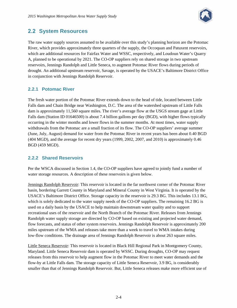
Jennings Randolph Reservoir: This reservoir is located in the far northwest corner of the Potomac River basin, bordering Garrett County in Maryland and Mineral County in West Virginia. It is operated by the USACE’s Baltimore District Office. Storage capacity in the reservoir is 29.3 BG. This includes 13.1 BG, which is solely dedicated to the water supply needs of the CO-OP suppliers. The remaining 16.2 BG is used on a daily basis by the USACE to help maintain downstream water quality and to support recreational uses of the reservoir and the North Branch of the Potomac River. Releases from Jennings Randolph water supply storage are directed by CO-OP based on existing and projected water demand, flow forecasts, and status of other system reservoirs. Jennings Randolph Reservoir is approximately 200 miles upstream of the WMA and releases take more than a week to travel to WMA intakes during low-flow conditions. The drainage area of Jennings Randolph Reservoir is about 263 square miles.
Little Seneca Reservoir: This reservoir is located in Black Hill Regional Park in Montgomery County, Maryland. Little Seneca Reservoir dam is operated by WSSC. During droughts, CO-OP may request releases from this reservoir to help augment flow in the Potomac River to meet water demands and the flow-by at Little Falls dam. The storage capacity of Little Seneca Reservoir, 3.9 BG, is considerably smaller than that of Jennings Randolph Reservoir. But, Little Seneca releases make more efficient use of
2-4

2015 Washington Metropolitan Area Water Supply Study
system storage because the travel time for a release to reach Little Falls dam is only about a day. Little Seneca Reservoir’s drainage area is about 21 square miles.
Savage Reservoir: This reservoir is located on the Savage River in the headwaters of the Potomac River basin near Jennings Randolph Reservoir. The reservoir is owned by the Upper Potomac River Commission (UPRC). The UPRC operates the dam with guidance from USACE’s Baltimore District Office. The USACE determines release rates from Savage Reservoir in tandem with those from Jennings Randolph Reservoir. During CO-OP drought operations, the combined Jennings Randolph and Savage releases are used to meet a flow target, determined by CO-OP, at the USGS stream flow gage (Station ID 01598500) at Luke, Maryland. The storage capacity of Savage Reservoir is approximately 6.1 BG. The drainage area of Savage Reservoir is about 105 square miles. Savage Reservoir is also the water supply source for the Town of Westernport, Maryland (see Section 5.2.1.2 for details).
2.2.3 Additional Resources
Three off-Potomac River reservoirs are operated by WSSC and Fairfax Water. In addition, Loudoun Water plans to have a pumped storage reservoir, Quarry A, operational by 2021.
Patuxent reservoirs: WSSC operates two reservoirs in the neighboring Patuxent River watershed, Tridelphia Reservoir and T. Howard Duckett Reservoir (sometimes referred to as Rocky Gorge Reservoir). These reservoirs are operated in series and are treated in this study as a single source. Total combined usable storage capacity of these reservoirs is about 10.0 BG. WSSC uses the Patuxent reservoirs on a daily basis to supplement its Potomac withdrawals. The combined drainage area of these reservoirs is about 132 square miles.
Occoquan Reservoir: Fairfax Water operates this reservoir on the Occoquan River, which is within the Potomac basin, but outside the freshwater drainage area that supplies water to the intakes on the Potomac mainstem. The reservoir’s current storage capacity is estimated by ICPRB to be about 7.6 BG. Water from the Occoquan Reservoir is treated at Fairfax Water’s Griffith treatment plant and then distributed to customers in the eastern portion of Fairfax Water’s service area and to Prince William County. Fairfax Water has a limited ability to transfer water from the Griffith plant to the western portion of its service area, at a rate of up to 35 MGD. The drainage area of Occoquan Reservoir is about 592 square miles.
Quarry A: Loudoun Water is reconfiguring a retired rock quarry for use as a raw water storage facility, planned to be operational in 2021. The quarry is located near Loudoun Water’s new water treatment plant adjacent to Goose Creek. The quarry’s capacity is expected to be 1.0 BG or greater. It will be filled with water pumped from the Potomac River and will be used to supplement Loudoun Water’s supply during low flow conditions.
2-5
2015 Washington Metropolitan Area Water Supply Study
3 Annual Demand Forecast
Introduction
In order to predict whether or not the current WMA water supply system will be able to meet demands in 2040, estimates of future annual water demand are made for all WMA suppliers. These annual average demand forecasts can be combined with models of daily variations in demand (Chapter 4) to simulate daily WMA water demand for a given forecast year. The resulting daily demand simulation models are incorporated into CO-OP’s water supply planning model, PRRISM, which is described in detail in Chapter 5. PRRISM is used to evaluate, on a daily basis, whether available water is sufficient to meet demand (Chapter 8).
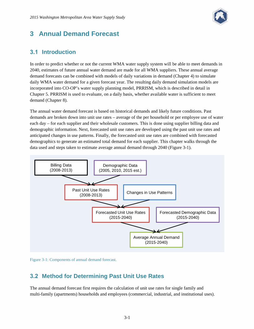
The annual water demand forecast is based on historical demands and likely future conditions. Past demands are broken down into unit use rates – average of the per household or per employee use of water each day – for each supplier and their wholesale customers. This is done using supplier billing data and demographic information. Next, forecasted unit use rates are developed using the past unit use rates and anticipated changes in use patterns. Finally, the forecasted unit use rates are combined with forecasted demographics to generate an estimated total demand for each supplier. This chapter walks through the data used and steps taken to estimate average annual demand through 2040 (Figure 3-1).
Figure 3-1: Components of annual demand forecast.
Method for Determining Past Unit Use Rates
The annual demand forecast first requires the calculation of unit use rates for single family and multi-family (apartments) households and employees (commercial, industrial, and institutional uses).
Past Unit Use Rates(2008-2013)
Billing Data(2008-2013)
Demographic Data(2005, 2010, 2015 est.)
Forecasted Unit Use Rates(2015-2040)
Changes in Use Patterns
Forecasted Demographic Data(2015-2040)
Average Annual Demand(2015-2040)
3-1

2015 Washington Metropolitan Area Water Supply Study
These three categories are used because they each have their own water use characteristics and trends. Calculating unit use rates for each requires disaggregated water use billing data from each supplier, including wholesale customers, and demographic data specific to the area served by the corresponding supplier. Each component of this calculation is explained below.
3.2.1 Utility Billing Data
The WMA suppliers and wholesale customers provided billing data, as available, for the period 2008-2013. Each supplier tracks and bills end users differently. In order to calculate unit use rates for this study’s single family households (SFH), multi-family households (MFH), and employee (EMP) categories, assumptions had to be made to put the billing data into these same categories. Appendix B explains this process in detail.
Data were either received as an annual number or aggregated into one from quarterly or fiscal year billing cycle data. The number and type of end user categories varied among suppliers. Some only had a residential and a commercial category; whereas, others had multiple categories for different types of residences and commercial activities.
In addition to the billing data, each supplier provided the amount of water produced and/or purchased and an estimate of unmetered water. Unmetered water can include water used to flush system pipes and clean tanks, fire hydrant use, or water lost to leaks, among other possibilities. It is also referred to as unaccounted for and non-revenue water. An estimate of unmetered water was made by calculating the difference between the amount of water produced and/or purchased and that billed to wholesale customers or end users. Unmetered water does not include water treatment plant production loss, which is defined in this study as the difference between withdrawals and production (see Section 5.5 for more information).
3.2.2 Current & Past Demographic Information
The second input into the unit use calculation is the number of single family households, multi-family households, and employees in each supplier’s service area. MWCOG gathers total household (occupied housing units), employee, and population data for WMA jurisdictions for the purpose of providing forecasts (Section 3.6.1). These data are available in five-year increments, so figures for 2008, 2009, 2011, 2012, and 2013 had to be interpolated. Round 7.2 (MWCOG, 2009) data were used for 2005 and Round 8.3 (MWCOG, 2014) data were used for 2010 and 2015 values.
3.2.2.1 Mapping to Service Area Boundaries
Since unit use rates are needed by supplier service area, but MWCOG data are by county and municipal jurisdiction, an additional step is needed to determine the demographics specific to each service area. This requires knowing the boundaries of each supplier’s service area and where they intersect with MWCOG’s planning units, known as traffic analysis zones (TAZ). TAZs are used throughout the country as geographic units for analyzing traffic patterns. They are the unit for which MWCOG reports the number of households, employees, and population.
3-2

2015 Washington Metropolitan Area Water Supply Study
The 2013 areas served by the suppliers and their wholesale customers are shown in Figure 3-2. Suppliers either provided updated GIS files of their service area boundary (Fairfax Water, WSSC, Rockville) or confirmed that there had been no changes since Part 1 of CO-OP’s 2010 water supply forecast (Ahmed et al., 2010, herein referred to as Part 1 of the 2010 demand study).
Figure 3-2: Areas served by water suppliers in the WMA in 2013. (Note that Vienna became a wholesale customer of Fairfax Water in 2013. Figure 3-4 reflects this and additional changes that occurred in 2014.)
To determine which TAZs are completely or partially within each service area, ESRI’s ArcMap™ was used to estimate a ratio of the area within a TAZ served by a supplier. For the TAZs that were not completely within an area served by one of the WMA water suppliers, it was assumed that the number of units (households, employees, or population) was allocated based on an area ratio. For example, if 50 percent of the area in a TAZ was within the area served by WSSC, then 50 percent of its households, employees, and population were assumed to be customers of WSSC.
To test this assumption, WSSC’s area served footprint and the overlapping TAZs were exported to Google Earth and overlaid on satellite imagery in order to survey visible households. If a TAZ was only
3-3

2015 Washington Metropolitan Area Water Supply Study
partially within the service area, the satellite image was used to estimate the percentage of households within the TAZ that were actually within the area. Both the original and the altered area ratios were applied to the TAZ data but only a small difference in the total number of households was found. Therefore, it was decided that the unadjusted area ratios were sufficient.
Once the ratios were applied to the TAZ data, the number of households, employees, and population for each service area were summed (Appendix B).
3.2.2.2 Dwelling Unit Ratios
The MWCOG data only supplies the total number of households within a TAZ, not disaggregated numbers of SFH and MFH. The disaggregated numbers are required to calculate the unit use rates for the two categories. In order to estimate the number of SFH and MFH, dwelling unit ratios are used. The dwelling unit ratio (DUR) is the number of single family households divided by the number of multi-family households.
Estimates of SFH and MFH were obtained or estimated from each jurisdiction’s planning agency or the U.S. Census Bureau. For suppliers that serve more than one county or that serve a portion of a county, an attempt was made to only include the households within the areas served by those suppliers. Often jurisdictions did not breakout these numbers by TAZ or planning area and a jurisdiction-wide number had to be used.
The ratios were applied to the 2010 and 2015 MWCOG data to estimate the number of SFH and MFH. The MWCOG numbers are used to maintain consistency with the numbers used in the annual demand forecast. Each supplier’s DUR and any assumptions are listed in Appendix B.
SFH and MFH calculations were done for 2010 and 2015. These numbers were used to interpolate estimated values for 2011-2013. To estimate 2008 and 2009 numbers, 2005 figures from Part 1 of the 2010 demand study were interpolated with this study’s 2010 estimate. The results are also available in Appendix B.
3.2.3 Past Unit Use Rates The billing and demographic data described above were used to calculate unit use rates for the years of available data (Table 3-1). These rates represent average daily water use by end user category in gallons per day (gpd). Unit use factors are calculated by dividing the total amount of water used per user category by the number of units (SFH, MFH, or EMP).
3-4

2015 Washington Metropolitan Area Water Supply Study
Table 3-1: Unit use values by water supplier (gpd).
Water Supplier 2008 2009 2010 2011 2012 2013
SFH MFH EMP SFH MFH EMP SFH MFH EMP SFH MFH EMP SFH MFH EMP SFH MFH EMP
Fairfax Water - Dulles International Airport (201.4) (163.3) 37.5 (195.5) (162.7) 34.9 (204.8) (161.9) 34.4 (197.6) (166.7) 34.8 (190.1) (155.5) 32.9 (184.0) (161.2) 32.9
Fairfax Water - Fort Belvoir (201.4) (163.3) 57.5 (195.5) (162.7) 48.9 (204.8) (161.9) 50.5 (197.6) (166.7) 47.9 (190.1) (155.5) 48.9 (184.0) (161.2) 38.7
Fairfax Water - Town of Herndon 165.0 49.5 155.0 46.6 160.3 49.3 151.9 48.5 144.9 45.3 127.2 45.4
Fairfax Water - Loudoun Water 221.9 157.2 50.5 208.8 150.0 45.0 220.5 146.8 50.3 202.0 141.0 47.6 202.3 137.7 52.8 191.0 139.2 47.4
Fairfax Water - Prince William County Service Authority
(221.9) (157.2) 51.6 (208.8) (150.0) 59.6 (220.5) (146.8) 43.4 (202.0) (141.0) 56.7 (202.3) (137.7) 52.6 (191.0) (139.2) 39.6
Fairfax Water – Retail customers 201.4 163.3 41.2 195.5 162.7 39.2 204.8 161.9 40.6 197.6 166.7 39.8 190.1 155.5 37.3 184.0 161.2 34.2
Fairfax Water - Virginia American Alexandria (201.4) (163.3) 20.5 (195.5) (162.7) 17.7 (204.8) (161.9) 22.6 (197.6) (166.7) 17.4 (190.1) (155.5) 23.4 (184.0) (161.2) 14.7
Fairfax Water - Virginia American Dale City1 (201.4) (163.3) 116.2 (195.5) (162.7) 33.5 (204.8) (161.9) 21.8 (197.6) (166.7) 14.2 (190.1) (155.5) 35.7 (184.0) (161.2) 18.5
Aqueduct - Arlington County DES 158.1 95.8 39.8 158.2 89.9 40.3 155.6 91.8 40.7 151.6 88.2 37.3 149.1 84.8 36.0 145.6 83.0 35.6
Aqueduct - City of Falls Church DES (201.4) (163.3) 47.1 (195.5) (162.7) 44.2 (204.8) (161.9) 40.6
Aqueduct - Vienna PWD (201.4) (163.3) 13.9 Aqueduct - DC Water 175.1 121.0 58.5 169.4 113.3 55.3 171.7 109.2 54.3 167.4 105.2 55.0 157.2 98.9 53.3 151.2 96.1 48.9
Aqueduct - Arlington - Fort Myer (201.4) (163.3) 63.0 (195.5) (162.7) 46.2 (204.8) (161.9) 41.0 (197.6) (166.7) 36.6 (190.1) (155.5) 42.9 (184.0) (161.2) 95.6
WSSC 182.5 154.5 40.0 165.6 154.9 36.0 166.3 159.1 40.3 161.9 153.6 41.0 158.1 133.6 46.0 155.7 138.5 41.6
City of Rockville DPW 157.8 142.0 25.9 156.3 140.7 20.3 149.0 134.2 26.9 149.2 Notes: Values in parenthesis are assumed, based on values from another supplier. Blank cells indicate no data or insufficient data were available to calculate the unit use rate. 1The value was calculated using the standard method for this section. See Appendix B for details.
3-5

2015 Washington Metropolitan Area Water Supply Study
3.2.4 Unit Use Trends
Unit use values fluctuate from year to year due to factors such as weather, demographic and economic conditions, and minor variations in estimation methods. Unit use factors are also expected to exhibit long-term trends because of changes in customer end use behavior.
Unit use factors calculated in the current and past studies are shown in Table 3-2 and graphed in Figure 3-3 for Fairfax Water (retail customers only), Aqueduct (DC Water customers only), and WSSC. Least square regression analyses indicate that SFH and MFH unit use for all three suppliers, as well as employee unit use for Fairfax Water and Aqueduct, have decreased significantly over 2002-2013, at the 95 percent confidence level (i.e., all p-values less than 0.05). The greatest rates of decline are for single family households and for Aqueduct and WSSC multi-family households.
3-6

2015 Washington Metropolitan Area Water Supply Study
Table 3-2: Unit use factors calculated in past and current studies (gpd).
Year Fairfax Water
(retail customers only) Aqueduct
(DC Water customers only) WSSC
SFH MFH EMP SFH MFH EMP SFH MFH EMP
19901 240.0 177.0 44.0 325.0 315.0 50.0 241.0 224.0 58.0
19952 229.0 156.0 47.0 237.0 237.0 50.0 249.0 233.0 53.0
19983 218.6 191.8 45.8 304.4 304.4 44.8 181.8 183.8 44.2
19993 161.0 171.1 42.9
20004 227.0 165.0 44.0 279.0 279.0 60.7 179.0 184.0 45.0
20025 241.5 171.1 49.9 168.2 172.9 58.1 185.0 173.4 45.9
20035 207.1 167.5 47.8 184.7 156.8 55.8 183.7 174.3 44.1
20045 206.4 158.9 45.1 169.6 159.8 56.9 178.9 175.3 46.6
20056 206.4 170.0 41.8 177.5 140.4 58.6 179.6 162.6 49.0
20066 211.2 167.5 42.3 174.7 137.9 61.5 185.7 154.2 44.0
20076 227.6 167.8 44.4 169.9 132.9 60.2 186.9 152.2 42.5
20087 201.4 163.3 41.2 175.1 121.0 58.5 182.5 154.5 40.0
20097 195.5 162.7 39.2 169.4 113.3 55.3 165.6 154.9 36.0
20107 204.8 161.9 40.6 171.7 109.2 54.3 166.3 159.1 40.3
20117 197.6 166.7 39.8 167.4 105.2 55.0 161.9 153.6 41.0
20127 190.1 155.5 37.3 157.2 98.9 53.3 158.1 133.6 46.0
20137 184.0 161.2 34.2 151.2 96.1 48.9 155.7 138.5 41.6 1 1990 study results (Holmes and Steiner, 1990), based primarily on 1988 data. 2 1995 study results (Mullusky et al., 1996), based primarily on 1993 or 1994 data (WSSC results are for existing housing units). 3 From 2000 study spreadsheet. 4 Revised 2000 value reported in 2005 study (Kame’enui et al., 2005). 5 2004 results from 2005 study (Kame’enui et al., 2005); 2002 and 2003 results from 2005 study spreadsheet. 6 Part 1 of the 2010 study results (Ahmed et al., 2010). 7 Current study results.
3-7
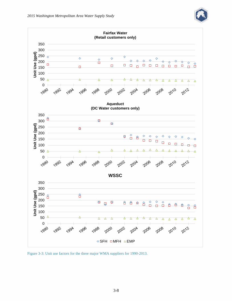
2015 Washington Metropolitan Area Water Supply Study
Figure 3-3: Unit use factors for the three major WMA suppliers for 1990-2013.
050
100150200250300350
Uni
t Use
(gpd
)Fairfax Water
(Retail customers only)
050
100150200250300350
Uni
t Use
(gpd
)
Aqueduct(DC Water customers only)
050
100150200250300350
Uni
t Use
(gpd
)
WSSC
SFH MFH EMP
3-8
2015 Washington Metropolitan Area Water Supply Study
3.2.4.1 Nationwide Trends
The recent trends in water use rates in the WMA are consistent with those seen across the country. Many, if not most, water suppliers are experiencing a decrease in SFH water use rates (Rockaway et al., 2011). Rockaway, et al. (2011) looked at water use trends in North America since 1992. They concluded that decreased water use can be attributed mainly to fewer people living in each household and the increasing use of low-flow appliances.
In a study of more than 3,000 homes, DeOreo and Mayer (2012) found the following water use rates in households built and sampled over different periods:
• 187 gpd in households sampled around 1999 and mostly built before the Energy Policy Act of 1992, which changed flow rates for some household fixtures;
• 162 gpd in existing households sampled around 2007; • 132 gpd in households built “off-the-shelf” after 2001; • 117 gpd in households retrofitted with high-efficiency appliances after 2001; and • 107 gpd in households built to WaterSense specifications after 2001.
The authors concluded that, “… there are reliable reductions in indoor water use in single-family residences that are due to changes in technology” (DeOreo and Mayer, 2012).
The reductions found in these and other studies are similar to those seen in the WMA. There is some question of what portion of the decrease starting in 2008 can be attributed to the national recession versus the use of more efficient appliances. The 2013 Tampa Bay Water Demand Management Plan (Hazen and Sawyer, 2013) came to two conclusions related to the recent recession:
• “It is important to note water use declined substantially following an all-time high in 2006. Although customer class growth is expected to resume, water use between WYs [water years] 2008-2010 was significantly impacted by economic recession. Water demand is not expected to recover to 2008 levels until 2015, at which time growth in projected water demand is expected to resume.
• During the economic recession, total retail demands decreased by 10 percent (20 MGD). Single-family experienced the greatest decrease at 13.5 MGD (12 percent), followed by nonresidential (11 percent, 5.2 MGD) and multifamily (4 percent, 1.6 MGD).”
Method for Forecasting Unit Use Rates The unit use rates calculated from billing and demographic data for 2008-2013, as shown in
Table 3-1, are the basis of the unit use forecast. From these past rates, a starting point for 2015 – the first year of the forecast in this study – was determined. Then, using information on potential changes in water use patterns, the unit use forecast through 2040 was developed. This section details the data and methods used for the forecast.
3-9
2015 Washington Metropolitan Area Water Supply Study
3.3.2 Selecting Unit Use Rate for Beginning of Demand Forecast Period
Different methods have been used in the previous demand studies to set the unit use rate for the first year in the forecast period. In the 2010 study, unit use factors from current and past studies for the WMA were compiled and analyzed to determine the most appropriate values (Section 3.8 of Part 1 of the 2010 demand study). Before the 2010 study, unit use factors for the beginning of the forecast period were generally approximated by the values calculated from the most recent years of available data. Sometimes minor adjustments would be made to account for weather effects. For this iteration of the study, the average of the unit rates for 2008-2013 (as available) was used for the 2015 forecast. This approach was selected because it recognizes the decrease in unit use, but assumes that some of it may be due to the economic recession, and that by 2015 use rates may return close to pre-recession levels.
3.3.3 Potential Changes in Customer Demand
Changes in water use behavior over a 30-year forecast period are difficult to predict and are a source of significant uncertainty in the demand forecasts. Changes in use over time can be attributed to a number of factors. For example, weather, retail rate structures, and government policies and regulations impact how much water is used. Block rate structures that increase charges as customers use more water can reduce the amount consumed. Policies, such as the Energy Policy Act of 1992, that require the use of more efficient plumbing fixtures can reduce water demand without requiring consumers to change their behavior. Government programs promoting voluntary water conservation, including the use of low-flow appliances as advocated for by the U.S. Environmental Protection Agency’s WaterSense program, may also affect consumer water use behavior. Long-term trends in regional temperature and precipitation which may result from global climate change could also have an impact on summer outdoor water use, which is a significant component of annual average demand. A detailed investigation of the potential impacts of global climate change on WMA water demand and resources was the subject of Part 2 of the 2010 demand study (Ahmed et al., 2013).
It is assumed that some of the reduction in unit use that has occurred in the WMA since the early 1990s can be attributed to the Energy Policy Act of 1992, and in more recent years to the WaterSense program as well. This study made assumptions based on the Energy Policy Act of 1992, WaterSense program, and consumer behavior literature to estimate reductions in household and employee unit use factors in the WMA (Appendix B). Changes over time in the number of households in the combined retail areas of the CO-OP suppliers were also incorporated.
The goal of this study was to estimate the average savings that could be expected for the entire WMA system, not to reflect estimates for any single supplier. More accurate estimates for each individual supplier could be computed based on supplier-specific data. The estimated savings computed in this study are independent of any changes that could be attributed to use behavior during the recession; they could be expected regardless. (Note that to limit the influence of the recession on future unit use estimates, the 2015 unit use estimates were averages of the unit use rates between 2008 and 2013.)
Specifically, estimated reductions were based on assumptions about residential water use rates; the number of existing households that have been remodeled; bathroom, fixture, and appliance replacement
3-10
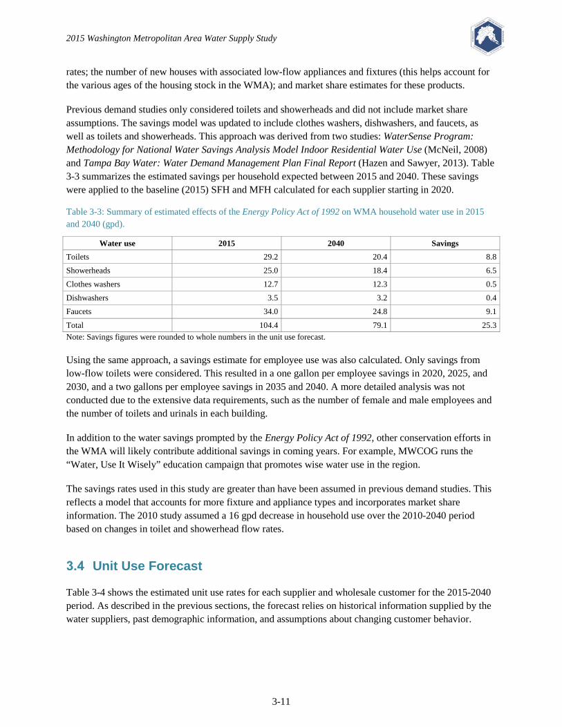
2015 Washington Metropolitan Area Water Supply Study
rates; the number of new houses with associated low-flow appliances and fixtures (this helps account for the various ages of the housing stock in the WMA); and market share estimates for these products.
Previous demand studies only considered toilets and showerheads and did not include market share assumptions. The savings model was updated to include clothes washers, dishwashers, and faucets, as well as toilets and showerheads. This approach was derived from two studies: WaterSense Program: Methodology for National Water Savings Analysis Model Indoor Residential Water Use (McNeil, 2008) and Tampa Bay Water: Water Demand Management Plan Final Report (Hazen and Sawyer, 2013). Table 3-3 summarizes the estimated savings per household expected between 2015 and 2040. These savings were applied to the baseline (2015) SFH and MFH calculated for each supplier starting in 2020.
Table 3-3: Summary of estimated effects of the Energy Policy Act of 1992 on WMA household water use in 2015 and 2040 (gpd).
Water use 2015 2040 Savings Toilets 29.2 20.4 8.8
Showerheads 25.0 18.4 6.5
Clothes washers 12.7 12.3 0.5
Dishwashers 3.5 3.2 0.4
Faucets 34.0 24.8 9.1
Total 104.4 79.1 25.3 Note: Savings figures were rounded to whole numbers in the unit use forecast.
Using the same approach, a savings estimate for employee use was also calculated. Only savings from low-flow toilets were considered. This resulted in a one gallon per employee savings in 2020, 2025, and 2030, and a two gallons per employee savings in 2035 and 2040. A more detailed analysis was not conducted due to the extensive data requirements, such as the number of female and male employees and the number of toilets and urinals in each building.
In addition to the water savings prompted by the Energy Policy Act of 1992, other conservation efforts in the WMA will likely contribute additional savings in coming years. For example, MWCOG runs the “Water, Use It Wisely” education campaign that promotes wise water use in the region.
The savings rates used in this study are greater than have been assumed in previous demand studies. This reflects a model that accounts for more fixture and appliance types and incorporates market share information. The 2010 study assumed a 16 gpd decrease in household use over the 2010-2040 period based on changes in toilet and showerhead flow rates.
Unit Use Forecast
Table 3-4 shows the estimated unit use rates for each supplier and wholesale customer for the 2015-2040 period. As described in the previous sections, the forecast relies on historical information supplied by the water suppliers, past demographic information, and assumptions about changing customer behavior.
3-11
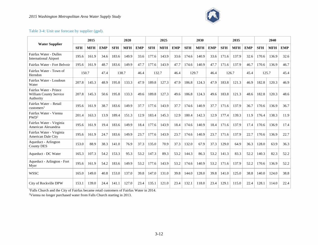
2015 Washington Metropolitan Area Water Supply Study
Table 3-4: Unit use forecast by supplier (gpd).
Water Supplier 2015 2020 2025 2030 2035 2040
SFH MFH EMP SFH MFH EMP SFH MFH EMP SFH MFH EMP SFH MFH EMP SFH MFH EMP
Fairfax Water - Dulles International Airport 195.6 161.9 34.6 183.6 149.9 33.6 177.6 143.9 33.6 174.6 140.9 33.6 171.6 137.9 32.6 170.6 136.9 32.6
Fairfax Water - Fort Belvoir 195.6 161.9 48.7 183.6 149.9 47.7 177.6 143.9 47.7 174.6 140.9 47.7 171.6 137.9 46.7 170.6 136.9 46.7
Fairfax Water - Town of Herndon 150.7 47.4 138.7 46.4 132.7 46.4 129.7 46.4 126.7 45.4 125.7 45.4
Fairfax Water - Loudoun Water 207.8 145.3 48.9 195.8 133.3 47.9 189.8 127.3 47.9 186.8 124.3 47.9 183.8 121.3 46.9 182.8 120.3 46.9
Fairfax Water - Prince William County Service Authority
207.8 145.3 50.6 195.8 133.3 49.6 189.8 127.3 49.6 186.8 124.3 49.6 183.8 121.3 48.6 182.8 120.3 48.6
Fairfax Water – Retail customers1 195.6 161.9 38.7 183.6 149.9 37.7 177.6 143.9 37.7 174.6 140.9 37.7 171.6 137.9 36.7 170.6 136.9 36.7
Fairfax Water - Vienna PWD2 201.4 163.3 13.9 189.4 151.3 12.9 183.4 145.3 12.9 180.4 142.3 12.9 177.4 139.3 11.9 176.4 138.3 11.9
Fairfax Water - Virginia American Alexandria 195.6 161.9 19.4 183.6 149.9 18.4 177.6 143.9 18.4 174.6 140.9 18.4 171.6 137.9 17.4 170.6 136.9 17.4
Fairfax Water - Virginia American Dale City 195.6 161.9 24.7 183.6 149.9 23.7 177.6 143.9 23.7 174.6 140.9 23.7 171.6 137.9 22.7 170.6 136.9 22.7
Aqueduct - Arlington County DES 153.0 88.9 38.3 141.0 76.9 37.3 135.0 70.9 37.3 132.0 67.9 37.3 129.0 64.9 36.3 128.0 63.9 36.3
Aqueduct - DC Water 165.3 107.3 54.2 153.3 95.3 53.2 147.3 89.3 53.2 144.3 86.3 53.2 141.3 83.3 52.2 140.3 82.3 52.2
Aqueduct - Arlington - Fort Myer 195.6 161.9 54.2 183.6 149.9 53.2 177.6 143.9 53.2 174.6 140.9 53.2 171.6 137.9 52.2 170.6 136.9 52.2
WSSC 165.0 149.0 40.8 153.0 137.0 39.8 147.0 131.0 39.8 144.0 128.0 39.8 141.0 125.0 38.8 140.0 124.0 38.8
City of Rockville DPW 153.1 139.0 24.4 141.1 127.0 23.4 135.1 121.0 23.4 132.1 118.0 23.4 129.1 115.0 22.4 128.1 114.0 22.4 1Falls Church and the City of Fairfax became retail customers of Fairfax Water in 2014. 2Vienna no longer purchased water from Falls Church starting in 2013.
3-12
2015 Washington Metropolitan Area Water Supply Study
Method for Developing the Annual Demand Forecast
Forecasting the total annual demand for each supplier involves multiplying the unit use rates from Table 3-4 above by the forecasts of the number of SFH, MFH, and EMP in each supplier’s area served and adding in assumptions for wholesale sales and unmetered water use. Unmetered water can include distribution system leaks and water used for fire suppression, construction, parks, and system and tank flushing. It does not include losses incurred during production. This section explains the development of the demographic forecast and unmetered water use assumption. This method is developed to be general enough to apply to all the region’s suppliers. Most suppliers conduct their own demand forecasts that often account for specific, local conditions that may lead to different results than the ones used in this study.
3.5.1 Demographic Forecast
Household, employment, and population projections for each water supplier’s area served are based on the MWCOG Round 8.3 Cooperative Forecast (MWCOG, 2014) and on a delineation of the current and future areas served by water suppliers using GIS tools. When available, the number of SFH and MFH in each jurisdiction was obtained to calculate the dwelling unit ratio (the number of SFH divided by the number of MFH) for each area served. In turn, the DUR was used to separate the MWCOG total household forecasts into the number of SFH and MFH.
The MWCOG forecast is developed through a cooperative process involving MWCOG and local government agencies. The Cooperative Forecasting Program, established in 1975 and administered by MWCOG, allows for coordinated local and regional planning using common assumptions about future growth and development. The forecast available at the beginning of this study, Round 8.3, for the period 2010-2040, was approved by the MWCOG Board of Directors in July 2014.
The development of the MWCOG forecast uses both a regional econometric model and bottom-up approach undertaken by local planning agencies. The econometric model is based on national and local economic and demographic trends, while the local planning agencies rely more on development and transportation plans, in addition to local economic and demographic trends. After these two forecasts have been independently completed, they are reconciled through MWCOG’s Cooperative Forecasting and Data Subcommittee and approved by MWCOG’s Board of Directors. The final product is an estimate of population, employees, and households as distributed by TAZ. Each county has several hundred TAZs, which allows for a forecast of water demand at the TAZ level by areas served by each supplier. In the WMA (as defined by this report) there are currently 2,567 TAZs of varying size. TAZs tend to be smaller closer to the urban core (i.e. D.C. has the most TAZs of all jurisdictions in the area). More information on the development of this forecast can be found at MWCOG’s website: www.mwcog.org.
3.5.1.1 Future Service Area Boundaries
The future extent of each area served by suppliers is difficult to predict. These estimations can be based on known physical constraints of the water supply system or on county zoning maps and comprehensive
3-13

2015 Washington Metropolitan Area Water Supply Study
plans. WSSC provided ICPRB with a future service area map which very slightly increased in size. Fairfax Water provided a map that detailed the incorporation of the City of Fairfax and the City of Falls Church into their retail service area in 2014. The remaining suppliers indicated no anticipated changes to their current area served. Figure 3-4 shows the anticipated future extent of each supplier’s service area.
Figure 3-4: Areas served by suppliers in the WMA in 2014 and beyond.
Using the updated service area boundaries, an analysis of the TAZs in each service area was done following the same method explained in Section 3.2.2.1. Once this process was complete, the population, household, and employee data for each area were extracted from the TAZ data (Table 3-5). Overall, Round 8.3 indicates continued growth throughout the area served by the WMA suppliers and their wholesale customers (Table 3-6). Fairfax Water is predicted to experience the most growth of all the suppliers over the next 25 years. The largest expected gain for Fairfax Water is again in the number of employees, which is predicted to grow by 47 percent between 2015 and 2040. Overall, the forecast indicates an increase in the number of households by 26 percent, employees by 36 percent, and population by 23 percent.
While Round 8.3 continues to indicate growth in the region, a comparison of the 2010 forecast in Round 7.2 (used in Part 1 of the 2010 demand study) and the estimated actual 2010 numbers in Round 8.3 shows that the number of households and employees were not quite as large as anticipated, but the total population exceeded predictions by a small amount (Table 3-7 and Table 3-8).
3-14

2015 Washington Metropolitan Area Water Supply Study
The 2010 study had to consider other potential growth areas that were not incorporated into MWCOG’s Round 7.2 forecast. There are no similar areas in Round 8.3, so no special areas were considered.
3-15
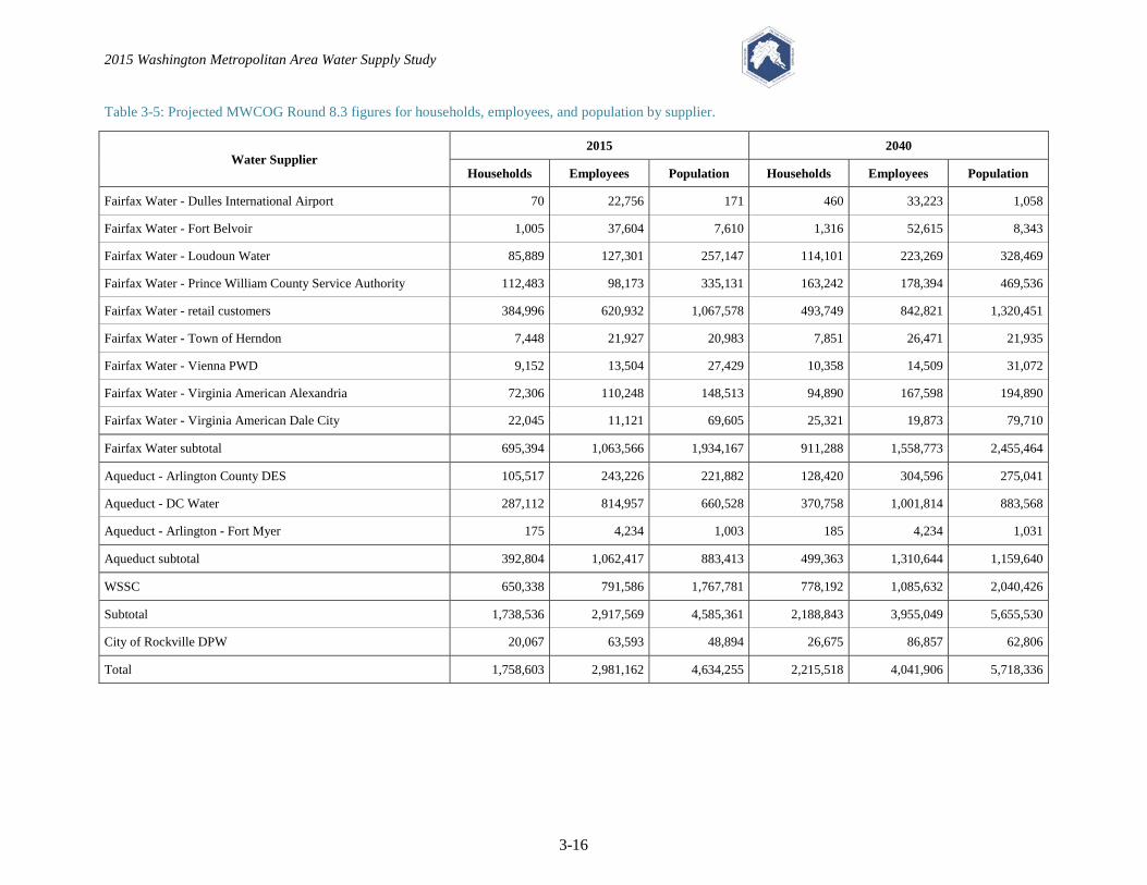
2015 Washington Metropolitan Area Water Supply Study
Table 3-5: Projected MWCOG Round 8.3 figures for households, employees, and population by supplier.
Water Supplier 2015 2040
Households Employees Population Households Employees Population
Fairfax Water - Dulles International Airport 70 22,756 171 460 33,223 1,058
Fairfax Water - Fort Belvoir 1,005 37,604 7,610 1,316 52,615 8,343
Fairfax Water - Loudoun Water 85,889 127,301 257,147 114,101 223,269 328,469
Fairfax Water - Prince William County Service Authority 112,483 98,173 335,131 163,242 178,394 469,536
Fairfax Water - retail customers 384,996 620,932 1,067,578 493,749 842,821 1,320,451
Fairfax Water - Town of Herndon 7,448 21,927 20,983 7,851 26,471 21,935
Fairfax Water - Vienna PWD 9,152 13,504 27,429 10,358 14,509 31,072
Fairfax Water - Virginia American Alexandria 72,306 110,248 148,513 94,890 167,598 194,890
Fairfax Water - Virginia American Dale City 22,045 11,121 69,605 25,321 19,873 79,710
Fairfax Water subtotal 695,394 1,063,566 1,934,167 911,288 1,558,773 2,455,464
Aqueduct - Arlington County DES 105,517 243,226 221,882 128,420 304,596 275,041
Aqueduct - DC Water 287,112 814,957 660,528 370,758 1,001,814 883,568
Aqueduct - Arlington - Fort Myer 175 4,234 1,003 185 4,234 1,031
Aqueduct subtotal 392,804 1,062,417 883,413 499,363 1,310,644 1,159,640
WSSC 650,338 791,586 1,767,781 778,192 1,085,632 2,040,426
Subtotal 1,738,536 2,917,569 4,585,361 2,188,843 3,955,049 5,655,530
City of Rockville DPW 20,067 63,593 48,894 26,675 86,857 62,806
Total 1,758,603 2,981,162 4,634,255 2,215,518 4,041,906 5,718,336
3-16
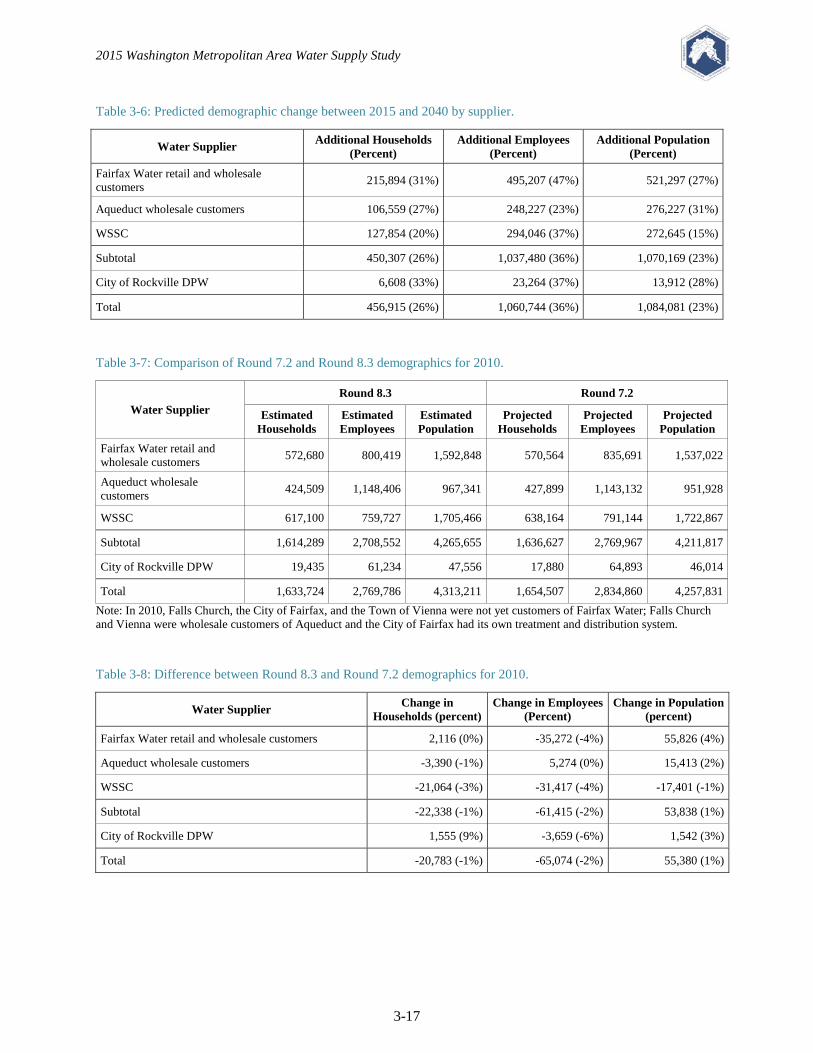
2015 Washington Metropolitan Area Water Supply Study
Table 3-6: Predicted demographic change between 2015 and 2040 by supplier.
Water Supplier Additional Households (Percent)
Additional Employees (Percent)
Additional Population (Percent)
Fairfax Water retail and wholesale customers 215,894 (31%) 495,207 (47%) 521,297 (27%)
Aqueduct wholesale customers 106,559 (27%) 248,227 (23%) 276,227 (31%)
WSSC 127,854 (20%) 294,046 (37%) 272,645 (15%)
Subtotal 450,307 (26%) 1,037,480 (36%) 1,070,169 (23%)
City of Rockville DPW 6,608 (33%) 23,264 (37%) 13,912 (28%)
Total 456,915 (26%) 1,060,744 (36%) 1,084,081 (23%)
Table 3-7: Comparison of Round 7.2 and Round 8.3 demographics for 2010.
Water Supplier Round 8.3 Round 7.2
Estimated Households
Estimated Employees
Estimated Population
Projected Households
Projected Employees
Projected Population
Fairfax Water retail and wholesale customers 572,680 800,419 1,592,848 570,564 835,691 1,537,022
Aqueduct wholesale customers 424,509 1,148,406 967,341 427,899 1,143,132 951,928
WSSC 617,100 759,727 1,705,466 638,164 791,144 1,722,867
Subtotal 1,614,289 2,708,552 4,265,655 1,636,627 2,769,967 4,211,817
City of Rockville DPW 19,435 61,234 47,556 17,880 64,893 46,014
Total 1,633,724 2,769,786 4,313,211 1,654,507 2,834,860 4,257,831 Note: In 2010, Falls Church, the City of Fairfax, and the Town of Vienna were not yet customers of Fairfax Water; Falls Church and Vienna were wholesale customers of Aqueduct and the City of Fairfax had its own treatment and distribution system.
Table 3-8: Difference between Round 8.3 and Round 7.2 demographics for 2010.
Water Supplier Change in Households (percent)
Change in Employees (Percent)
Change in Population (percent)
Fairfax Water retail and wholesale customers 2,116 (0%) -35,272 (-4%) 55,826 (4%)
Aqueduct wholesale customers -3,390 (-1%) 5,274 (0%) 15,413 (2%)
WSSC -21,064 (-3%) -31,417 (-4%) -17,401 (-1%)
Subtotal -22,338 (-1%) -61,415 (-2%) 53,838 (1%)
City of Rockville DPW 1,555 (9%) -3,659 (-6%) 1,542 (3%)
Total -20,783 (-1%) -65,074 (-2%) 55,380 (1%)
3-17

2015 Washington Metropolitan Area Water Supply Study
3.5.1.3 Forecasted Dwelling Unit Ratios
The same step that was used to divide the total number of MWCOG households into estimates of SFH and MFH to determine the historical unit use rates in Section 3.2.2.2 was taken to develop the demand forecasts. To complete this step, forecasts of dwelling unit ratios were needed (Table 3-9). These data were either provided by the jurisdiction or estimated from available data. The details of the data used and assumptions made are documented in Appendix B.
Table 3-9: Forecasted dwelling unit ratios for each jurisdiction.
Jurisdiction Water Supplier 2015 2020 2025 2030 2035 2040
Arlington County Arlington County, Fort Myer 0.52 0.48 0.45 0.43 0.42 0.40
City of Alexandria Virginia American Alexandria 0.38 0.36 0.35 0.33 0.32 0.31
City of Rockville City of Rockville 1.50 1.24 1.09 0.97 0.87 0.79
Dale City Virginia American Dale City 8.94 9.07 9.20 9.33 9.48 9.66
District of Columbia DC Water 0.59 0.59 0.59 0.59 0.59 0.59
Fairfax County Fairfax Water, Dulles Airport, Fort Belvoir 2.51 2.22 1.97 1.80 1.65 1.53
Loudoun County Loudoun Water 4.01 3.42 2.85 2.48 2.33 2.29
Montgomery County WSSC 1.88 1.74 1.61 1.44 1.34 1.27
Prince George's County WSSC 2.45 2.38 2.34 2.31 2.26 2.21
Prince William County Prince William County Service Authority 3.15 2.53 2.17 1.96 1.85 1.80
Town of Herndon Town of Herndon 2.15 2.15 2.15 2.15 2.15 2.15
Town of Vienna Town of Vienna 8.81 8.81 8.81 8.81 8.81 8.81 Note: See Appendix B for details on how each jurisdiction’s DUR was calculated.
3.5.2 Estimate of Unmetered Water Use
A water supplier’s average annual demand includes an estimate of unmetered water use. Unmetered use is calculated as the difference between the water produced at the treatment plant (or purchased at the wholesale level) and the water billed to customers. It is usually represented as a percent of the total amount produced or purchased. Each supplier’s past unmetered rate was calculated for the years of provided water use data (Appendix B). For the purposes of the forecasts, the past rates were averaged and applied to the forecasts for total SFH, MFH, and employee use. If the averaged rate was less than ten percent, ten percent was assumed. This provided a conservative planning-level estimate of future demand that accounts for increased losses as infrastructure ages, consistent with previous WMA demand studies. This assumption was made for Fairfax Water’s retail area, Herndon, and Vienna. Table 3-10 shows the rates used for each supplier.
3-18
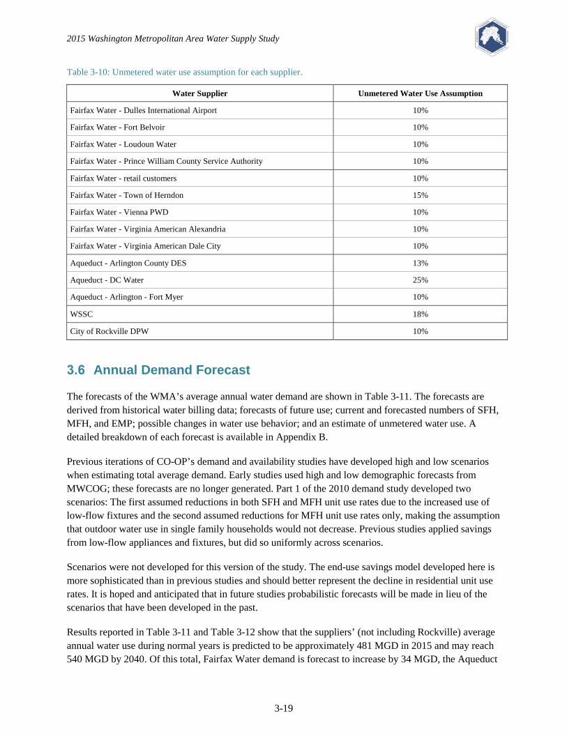
2015 Washington Metropolitan Area Water Supply Study
Table 3-10: Unmetered water use assumption for each supplier.
Water Supplier Unmetered Water Use Assumption
Fairfax Water - Dulles International Airport 10%
Fairfax Water - Fort Belvoir 10%
Fairfax Water - Loudoun Water 10%
Fairfax Water - Prince William County Service Authority 10%
Fairfax Water - retail customers 10%
Fairfax Water - Town of Herndon 15%
Fairfax Water - Vienna PWD 10%
Fairfax Water - Virginia American Alexandria 10%
Fairfax Water - Virginia American Dale City 10%
Aqueduct - Arlington County DES 13%
Aqueduct - DC Water 25%
Aqueduct - Arlington - Fort Myer 10%
WSSC 18%
City of Rockville DPW 10%
Annual Demand Forecast
The forecasts of the WMA’s average annual water demand are shown in Table 3-11. The forecasts are derived from historical water billing data; forecasts of future use; current and forecasted numbers of SFH, MFH, and EMP; possible changes in water use behavior; and an estimate of unmetered water use. A detailed breakdown of each forecast is available in Appendix B.
Previous iterations of CO-OP’s demand and availability studies have developed high and low scenarios when estimating total average demand. Early studies used high and low demographic forecasts from MWCOG; these forecasts are no longer generated. Part 1 of the 2010 demand study developed two scenarios: The first assumed reductions in both SFH and MFH unit use rates due to the increased use of low-flow fixtures and the second assumed reductions for MFH unit use rates only, making the assumption that outdoor water use in single family households would not decrease. Previous studies applied savings from low-flow appliances and fixtures, but did so uniformly across scenarios.
Scenarios were not developed for this version of the study. The end-use savings model developed here is more sophisticated than in previous studies and should better represent the decline in residential unit use rates. It is hoped and anticipated that in future studies probabilistic forecasts will be made in lieu of the scenarios that have been developed in the past.
Results reported in Table 3-11 and Table 3-12 show that the suppliers’ (not including Rockville) average annual water use during normal years is predicted to be approximately 481 MGD in 2015 and may reach 540 MGD by 2040. Of this total, Fairfax Water demand is forecast to increase by 34 MGD, the Aqueduct
3-19

2015 Washington Metropolitan Area Water Supply Study
by 13 MGD, and WSSC by 12 MGD. Most of the growth is expected in the employee category, followed by MFH. A decrease in total annual average demand in SFH is predicted. This is driven by decreasing unit use rates, assumed due to an increase use of low-flow fixtures and appliances, and fewer new single family homes. For the period 2015-2040, 191,863 more MFH than SFH are forecast.
Table 3-11: Forecast of average annual water demand by supplier, 2015-2040 (MGD).
Water Supplier 2015 2020 2025 2030 2035 2040
Fairfax Water - Dulles International Airport 0.880 1.003 1.126 1.209 1.227 1.271
Fairfax Water - Fort Belvoir 2.222 2.369 2.668 2.970 2.923 2.935
Fairfax Water - Loudoun Water 25.224 27.883 29.687 31.018 31.420 31.979
Fairfax Water - Prince William County Service Authority1 29.413 30.914 32.827 34.888 36.530 38.455
Fairfax Water - retail customers 105.146 104.711 108.496 112.839 115.298 119.407
Fairfax Water - Town of Herndon 2.485 2.423 2.435 2.466 2.467 2.517
Fairfax Water - Vienna PWD 2.196 2.094 2.093 2.113 2.115 2.156
Fairfax Water - Virginia American Alexandria 15.969 15.811 16.313 16.937 17.465 18.329
Fairfax Water - Virginia American Dale City 4.963 4.849 4.871 4.958 5.025 5.160
Fairfax Water subtotal 188.498 192.057 200.516 209.398 214.470 222.209
Aqueduct - Arlington County DES 23.811 23.904 24.224 24.607 24.220 24.497
Aqueduct - DC Water 101.311 101.794 104.870 108.503 110.104 113.334
Aqueduct - Arlington - Fort Myer 0.286 0.278 0.277 0.278 0.273 0.273
Aqueduct subtotal 125.408 125.976 129.371 133.388 134.597 138.104
WSSC – retail customers 161.028 158.239 160.473 165.035 167.697 172.913
WSSC – Charles County2 1.4 1.4 1.4 1.4 1.4 1.4
WSSC – Howard County2 5.0 5.0 5.0 5.0 5.0 5.0
WSSC subtotal 167.428 164.639 166.873 171.435 174.097 179.313
Fairfax Water, Aqueduct, WSSC Subtotal 481.334 482.672 496.760 514.221 523.164 539.626
City of Rockville DPW 4.962 4.894 5.014 5.266 5.407 5.668
Total 486.296 487.566 501.774 519.487 528.571 545.294 1Includes the 0.1 MGD sold to wholesale customers. 22015-2040 wholesale figures are based on total allowable amounts sold to Howard and Charles counties by WSSC.
3-20

2015 Washington Metropolitan Area Water Supply Study
Table 3-12: Change in average annual demand by water use category and supplier, 2015-2040 (MGD).
Water Supplier SFH MFH EMP Unmetered Total Difference
Fairfax Water - Dulles International Airport 0.040 0.019 0.296 0.036 0.391
Fairfax Water - Fort Belvoir -0.004 0.025 0.626 0.066 0.713
Fairfax Water - Loudoun Water 0.232 1.681 4.246 0.596 6.755
Fairfax Water - Prince William County Service Authority 1.442 3.076 3.702 0.822 9.042
Fairfax Water - retail customers -2.793 8.856 6.902 1.296 14.261
Fairfax Water - Town of Herndon -0.135 0.163 0.004 0.032
Fairfax Water - Vienna PWD -0.014 -0.007 -0.015 -0.004 -0.040
Fairfax Water - Virginia American Alexandria -0.064 1.433 0.777 0.214 2.360
Fairfax Water - Virginia American Dale City 0.036 -0.033 0.176 0.018 0.197
Fairfax Water subtotal -1.1925 15.050 16.792 3.046 33.695
Aqueduct - Arlington County DES -0.825 -0.311 1.741 0.081 0.686
Aqueduct - DC Water 1.691 -0.184 8.124 2.392 12.023
Aqueduct - Arlington - Fort Myer -0.003 -0.001 -0.008 -0.001 -0.013
Aqueduct subtotal 0.863 -0.496 9.857 2.472 12.696
WSSC -5.476 5.708 9.826 1.827 11.885
Fairfax Water, Aqueduct, WSSC Subtotal -5.8055 20.195 36.556 7.347 58.292
City of Rockville DPW -0.335 0.583 0.394 0.064 0.706
Total -6.1405 20.778 36.950 7.411 58.998 Note: Herndon's residential use savings are split in the totals for SFH and MFH savings.
Comparison of Annual Demand Forecast with Previous Estimates
Figure 3-5 compares the forecasted demands shown in Table 3-11, excluding Rockville, with results from previous studies done by ICPRB and other organizations (Ahmed et al., 2010; Kame'enui et al., 2005; Hagen and Steiner, 2000; Mullusky et al., 1996; Holmes and Steiner, 1990; USACE, 1975; MWCOG, as reported in USACE, 1983). It is clear from this figure that demand forecasts have consistently fallen over time. Throughout most of the past four decades, population has continued to grow in the WMA, but unit use values have fallen. The results from Part 1 of the 2010 demand study seemed to indicate that these decreasing trends in unit use might be leveling off. On the graph, this is illustrated by the position of the demand forecast lines for ICPRB’s 2005 and 2010 studies, which are close to one another. The 2015 forecast line shows that use rates have, in fact, not leveled off and have instead decreased since the last study. The difference between the 2040 annual demand forecast from Part 1 of 2010 study’s likely scenario and the 2015 scenario is approximately 70 MGD. Some of the decline can be attributed to the increased use of low-flow appliances and fixtures, but some of it is also likely due to the national recession. How much and whether or not rates will bounce back to pre-recession levels remains to be seen.
3-21

2015 Washington Metropolitan Area Water Supply Study
Figure 3-5: Comparison of the current study’s WMA annual average demand forecasts with forecasts from earlier studies.
0.0
1.0
2.0
3.0
4.0
5.0
6.0
200
300
400
500
600
700
800
900
1000
1960 1965 1970 1975 1980 1985 1990 1995 2000 2005 2010 2015 2020 2025 2030 2035 2040
Popu
latio
n (M
illion
s)
Dem
and
(MG
D)
MWCOG, 1975
Population
USACE, 1983
ICPRB, 1990
ICPRB, 1995
ICPRB, 2000
ICPRB, 2010 (high)
ICPRB, 2010
ICPRB, 2005
ICPRB, 2015
USACE, 1963
Actual Water Demands
3-22

2015 Washington Metropolitan Area Water Supply Study
4 Modeling Daily Variations in Water Demand
Water demand in the WMA varies with season, day of the week, and even hour of the day. In the summer and early fall, demand on any given day also depends on weather conditions, since people are more likely to water lawns and landscapes on hot, dry days. High summer demands often coincide with periods of low Potomac River flow, which falls to its lowest levels in September. In order to assess whether or not the current WMA water supply system will be able to meet future demands, seasonal and daily variations in demands need to be taken into account and combined with the average annual demand forecasts presented in Chapter 3.
In this study the terms “demand” and “production” are used interchangeably. In Chapter 3, average annual demand was by definition equal to the average annual production, since both include the “unmetered” or unbilled portion of water produced. Unmetered water was estimated as the difference between reported annual production by water treatment plants and reported customer demand estimated from billing data. Unmetered water includes many types of water uses that are not typically billed, such as water used by suppliers to flush water distribution systems or to clean tanks, and water used by municipalities or counties for firefighting or to maintain parks. It also includes water lost through leakage from the distribution system.
CO-OP’s planning model, PRRISM, incorporates water demand models which simulate the daily demands of each of the three CO-OP suppliers and also of Loudoun Water. (These demands include both retail and wholesale forecasts.) The models add daily variation to the annual demand forecasts described in Chapter 3. These daily demand models were developed using daily water production data for the years 1998-2013, provided by the four suppliers. In PRRISM, daily water demands are a function of:
• simulation year, • month, • season, • weather conditions, • day of the week, and • a daily error term based on an autoregressive integrated moving average (ARIMA) process.
PRRISM simulates monthly variations by applying empirically-derived monthly “production factors” to the annual demand forecasts to obtain monthly demand forecasts. Multiple least squares regression models are used to add variation due to weather conditions and day of the week. The sum of demand forecasts for the four suppliers is then further enhanced using an autoregressive integrated moving average (ARIMA) model, which adds information to the forecast not captured by the regression model. The models used in the current study include an independent multiple regression model for Loudoun Water demand, which had previously been based on Fairfax Water’s demand forecast.
This chapter describes the structure of the daily demand simulation models and the derivation from historical data of the model parameters used in PRRISM. The preparation of the raw data for the multiple regression and the ARIMA models is also discussed. Important features of the data preparation include the choice of predictor variables (independent variables), collation of data, preliminary analysis, detrending, and finally fitting the regression models for each supplier and season.
4-1
2015 Washington Metropolitan Area Water Supply Study
Data
The models used to simulate daily variations of WMA water demand are developed from the following data:
Daily production (MGD) records of water pumped from the treatment facilities of the three CO-OP suppliers and daily records of water purchased by Loudoun Water are used to estimate daily variations in demand. These data sets are used instead of billing data, which are relied upon for the average annual demand forecasts discussed in Chapter 3, because billing data is only available on a monthly, quarterly, or, in some cases, annual basis. Appendix A summarizes the production data as it was provided by each of the suppliers.
National Weather Service data includes daily maximum temperature (degrees Fahrenheit, oF), daily precipitation (inches), and number of consecutive days with precipitation less than 0.15 inches. These data sets came from records obtained from the National Climatic Data Center for Washington Reagan Airport (USW00013743), College Park (USC00181995), Frederick Police Barracks (USC00183348), Laurel 3 W (USC00185111), and Vienna (USC00448737).2 In order to represent the nonlinear response of demands to climate: (1) temperature was split so that different regression coefficients could be applied to temperatures greater than and less than 90oF. For temperatures lagged by more than one day, no partitioning was used; (2) Precipitation was capped at 0.2 inches for WSSC, and 0.3 inches for Aqueduct, Fairfax Water, and Loudoun Water. (See Section 5.6.4 of Part 1 of the 2010 study for more explanation on why this modification was made to the weather data.)
In addition, weekly and seasonal variations in user behavior are considered. Weekly variation in use is represented by day of the week, a variable in the multiple regression models. Instead of having variables represent seasonal influences, the multiple regression equations are separated into three independent analyses for spring, summer, and fall. Other social influences on water use are removed by detrending the raw data as described in Section 4.2.
The daily demand simulation models developed for the three main CO-OP suppliers are based on data for the time period of January 1, 1998, through December 31, 2013. The start and end year were chosen in order to include the 1999 drought and eliminate potentially out-of-date trends in production from earlier years. The year 2013 was the most recent full year of data at the time of the analysis. The models developed for Loudoun Water use a shorter time period of January 1, 2005, through December 31, 2013, because of a qualitative change in daily variation in the detrended purchased water between the earlier years and the selected period (discussed further in Section 4.3).
2 Fairfax Water precipitation is a composite of Vienna, Reagan, College Park, Laurel, and Frederick Police Barracks. WSSC precipitation is a composite of College Park, Laurel, Frederick Police Barracks, and Reagan. Aqueduct is a composite of Reagan, College Park, Laurel, and Frederick Police Barracks. The same temperature is used for all three locations and is based on a composite of Reagan, College Park, and Frederick Police Barracks. A composite time series is required to account for missing data. The priority of the data is based on the order in which it is listed above.
4-2
2015 Washington Metropolitan Area Water Supply Study
Removing the Long-term Time Trends
Long-term time trends are evident in the historical production data of all four suppliers. These trends are likely due to a combination of factors, including growth of the user populations, decreases in flow rates of plumbing fixtures and household appliances, and changes in economic conditions. These factors (with the exception of economic conditions) are included in the forecast of average annual water use, as described in Chapter 3. Therefore, these time trends are removed from the production data prior to the development of multiple regression equations to predict daily variations of demand from weather conditions and weekly and seasonal use patterns. This detrending procedure helps ensure stationarity in the mean of the data. Detrending is done by subtracting a time trend from the production data to obtain a set of residuals that are then added back to the most recent value of the original data. In this way, the influences on demand that are not explicitly accounted for in the multiple regression analyses (see Section 4.4) are removed.
The detrending procedure is modified from the method used by Steiner (1984), Kame’enui et al. (2005), and Ahmed et al. (2010). Instead of a linear model form for the time trend a composite model is used. The graphs of production data in Figure 4-1 and Figure 4-2 show that the data may be split into two regions. In the earlier portion of the data, a linear trend has historically been found to be appropriate, and that model form is maintained in the current study. However, at some point, the production data begins to slope downward. This later region is consistent with individual supplier accounts of decreasing water consumption rates. As discussed in Chapter 3, declining water consumption has been observed across the country and has been attributed to implementation of water saving fixtures and appliances, the effects of the recession, weather, and increased conservation (see Hunter et al., 2011 and Beecher, 2010). A quadratic model was found to provide a reasonable fit to this second region of the data. For the purpose of this study the boundary for the two regions was chosen as the beginning of 2008 (highlighted by the red point in Figure 4-1 and Figure 4-2), which is consistent with the onset of the “Great Recession.”
4-3

2015 Washington Metropolitan Area Water Supply Study
Figure 4-1: Production data (gray points) fitted to a linear-quadratic model (black line) with a break point (red point) in the beginning of 2008.
4-4
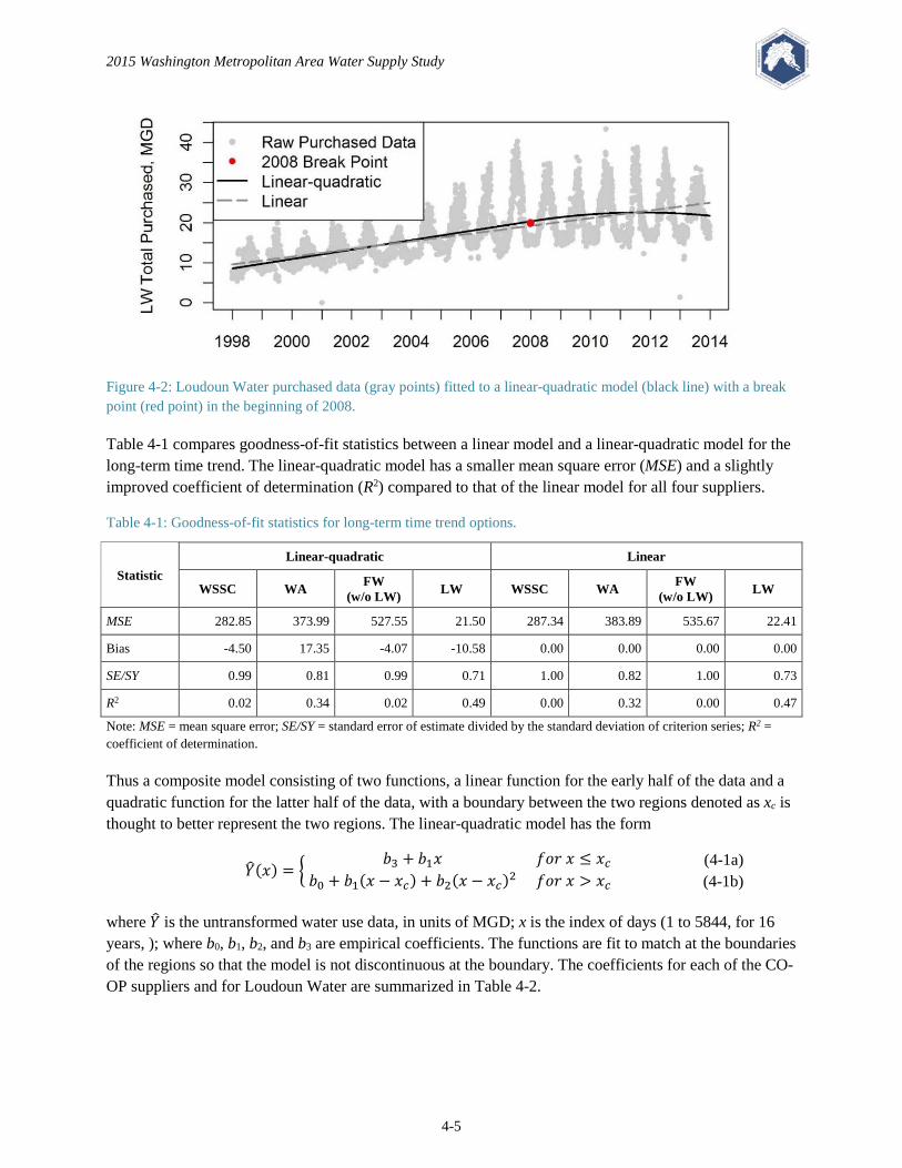
2015 Washington Metropolitan Area Water Supply Study
Figure 4-2: Loudoun Water purchased data (gray points) fitted to a linear-quadratic model (black line) with a break point (red point) in the beginning of 2008.
Table 4-1 compares goodness-of-fit statistics between a linear model and a linear-quadratic model for the long-term time trend. The linear-quadratic model has a smaller mean square error (MSE) and a slightly improved coefficient of determination (R2) compared to that of the linear model for all four suppliers.
Table 4-1: Goodness-of-fit statistics for long-term time trend options.
Statistic Linear-quadratic Linear
WSSC WA FW (w/o LW) LW WSSC WA FW
(w/o LW) LW
MSE 282.85 373.99 527.55 21.50 287.34 383.89 535.67 22.41
Bias -4.50 17.35 -4.07 -10.58 0.00 0.00 0.00 0.00
SE/SY 0.99 0.81 0.99 0.71 1.00 0.82 1.00 0.73
R2 0.02 0.34 0.02 0.49 0.00 0.32 0.00 0.47
Note: MSE = mean square error; SE/SY = standard error of estimate divided by the standard deviation of criterion series; R2 = coefficient of determination.
Thus a composite model consisting of two functions, a linear function for the early half of the data and a quadratic function for the latter half of the data, with a boundary between the two regions denoted as xc is thought to better represent the two regions. The linear-quadratic model has the form
𝑌𝑌�(𝑥𝑥) = � 𝑏𝑏3 + 𝑏𝑏1𝑥𝑥 𝑓𝑓𝑓𝑓𝑓𝑓 𝑥𝑥 ≤ 𝑥𝑥𝑐𝑐
𝑏𝑏0 + 𝑏𝑏1(𝑥𝑥 − 𝑥𝑥𝑐𝑐) + 𝑏𝑏2(𝑥𝑥 − 𝑥𝑥𝑐𝑐)2 𝑓𝑓𝑓𝑓𝑓𝑓 𝑥𝑥 > 𝑥𝑥𝑐𝑐 (4-1a)
(4-1b)
where 𝑌𝑌� is the untransformed water use data, in units of MGD; x is the index of days (1 to 5844, for 16 years, ); where b0, b1, b2, and b3 are empirical coefficients. The functions are fit to match at the boundaries of the regions so that the model is not discontinuous at the boundary. The coefficients for each of the CO-OP suppliers and for Loudoun Water are summarized in Table 4-2.
4-5

2015 Washington Metropolitan Area Water Supply Study
Table 4-2: Empirical coefficients for the linear-quadratic composite model for long-term trend in production for Equation (4-1a) and Equation (4-1b).
Water Supplier b0 b1 b2 b3
WSSC 1.69e2 1.25e3 -2.62e6 1.65e2
WA 1.61e2 -6.08e3 -3.88e6 1.83e2
FW (w/o LW) 1.36e2 2.35e-3 -3.52e-6 1.27e2
LW 2.03e1 3.22e-3 -1.18e-6 8.53e0
The last point on the long-term trend line, 𝑥𝑥′, is the long-term stationary mean, 𝑌𝑌�(𝑥𝑥′), to which all the residuals are added to form the detrended time series (see Figure 4-3 and Figure 4-4 in Section 4.3). The result is a demand series that represents current conditions from which forecasts can be made and from which model parameters can be estimated. The point on the regression line corresponding to the most recent observation can be represented by Equation (4-2):
𝑌𝑌�(𝑥𝑥′) = 𝑏𝑏0 + 𝑏𝑏1(𝑥𝑥′ − 𝑥𝑥𝑐𝑐) + 𝑏𝑏2(𝑥𝑥′ − 𝑥𝑥𝑐𝑐)2 (4-2)
where x’ is the time index of the most recent observation, which is 5844 and corresponds to December 31, 2013. Table 4-3 shows that the linear-quadratic formula in Equation (4-2) produces a long-term stationary mean that is lower than those obtained through the 2010 study and the 2015 study linear formulas.
Table 4-3: Comparison of the 2010 and 2015 ICPRB studies’ long-term stationary means (MGD).
Water Supplier 2010 Linear 𝒀𝒀�(𝒙𝒙′)
2015 Linear 𝒀𝒀�(𝒙𝒙′)
2015 Linear-Quadratic 𝒀𝒀�(𝒙𝒙′)
2013 Mean Annual Production from data
WSSC 169.07 166.51 159.34 158.63
WA 159.96 139.58 128.97 133.52
FW (no LW) N/A 133.79 124.15 125.53
LW N/A 24.93 21.69 21.80
Monthly Mean Production
Daily variation in demand was chosen as the criterion variable for the multiple regression analyses. This variable was computed from the detrended production data by using monthly production factors and the long-term stationary means. Definitions describing how this was done follow:
Monthly production factors are the ratio of average monthly production to average annual production, where the averaging period is 1998-2013. These are used to disaggregate annual production into monthly production. Values are provided in Table 4-4. (A trend analysis verifying that the assumption of stationarity in monthly production factors is acceptable is provided in Appendix C.)
Long-term monthly means are the product of monthly production factors and the long-term stationary means from Table 4-4.
4-6

2015 Washington Metropolitan Area Water Supply Study
Daily variation in demand is the residual difference between the detrended daily production data and the long-term monthly means. The two time series are compared in Figure 4-3 and Figure 4-4.
Using daily variation as the criterion variable enables simulations of potential daily differences from future monthly productions. When the daily variation estimates are added back to the monthly disaggregation of the annual production forecast the result is the daily production forecast.
Table 4-4: Production factors and monthly means by supplier.
Month
Average Monthly Production Factors Long-term Monthly Means, MGD
WSSC (1998-2013)
WA (1998-2013)
FW - no LW (1998-
2013)
LW (2005-2013) WSSC WA FW - no
LW LW
Jan 0.94 0.94 0.88 0.76 150.52 121.61 108.75 16.44
Feb 0.94 0.94 0.85 0.76 149.11 121.31 105.90 16.49
Mar 0.93 0.92 0.86 0.77 147.94 119.04 106.51 16.77
Apr 0.96 0.94 0.93 0.93 152.31 121.78 115.28 20.09
May 1.02 0.99 1.04 1.05 162.84 127.37 128.76 22.88
Jun 1.09 1.07 1.14 1.28 173.15 138.52 141.83 27.74
Jul 1.12 1.14 1.22 1.39 178.54 147.46 151.83 30.22
Aug 1.10 1.13 1.20 1.34 175.12 146.36 148.70 29.06
Sep 1.05 1.06 1.11 1.18 167.31 137.24 137.25 25.66
Oct 0.98 0.99 0.99 0.94 155.79 127.26 122.73 20.44
Nov 0.94 0.94 0.90 0.81 149.96 121.16 111.74 17.61
Dec 0.93 0.91 0.88 0.77 148.72 117.96 109.20 16.60
Annual 159.28 128.92 124.04 21.67
4-7

2015 Washington Metropolitan Area Water Supply Study
Figure 4-3: Daily production data detrended and compared to the monthly disaggregation of the long-term stationary mean.
4-8
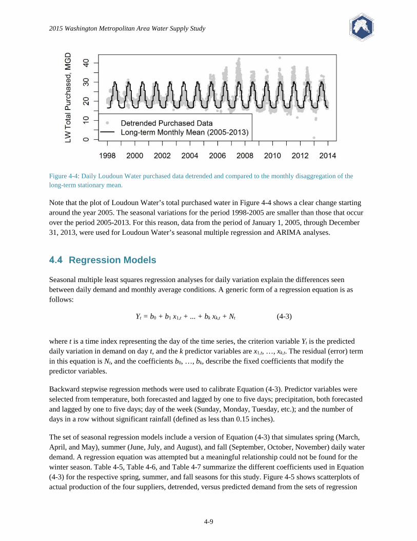
2015 Washington Metropolitan Area Water Supply Study
Figure 4-4: Daily Loudoun Water purchased data detrended and compared to the monthly disaggregation of the long-term stationary mean.
Note that the plot of Loudoun Water’s total purchased water in Figure 4-4 shows a clear change starting around the year 2005. The seasonal variations for the period 1998-2005 are smaller than those that occur over the period 2005-2013. For this reason, data from the period of January 1, 2005, through December 31, 2013, were used for Loudoun Water’s seasonal multiple regression and ARIMA analyses.
Regression Models
Seasonal multiple least squares regression analyses for daily variation explain the differences seen between daily demand and monthly average conditions. A generic form of a regression equation is as follows:
Yt = b0 + b1 x1,t + ... + bk xk,t + Nt (4-3)
where t is a time index representing the day of the time series, the criterion variable Yt is the predicted daily variation in demand on day t, and the k predictor variables are x1,t, …, xk,t. The residual (error) term in this equation is Nt, and the coefficients b0, …, bk, describe the fixed coefficients that modify the predictor variables.
Backward stepwise regression methods were used to calibrate Equation (4-3). Predictor variables were selected from temperature, both forecasted and lagged by one to five days; precipitation, both forecasted and lagged by one to five days; day of the week (Sunday, Monday, Tuesday, etc.); and the number of days in a row without significant rainfall (defined as less than 0.15 inches).
The set of seasonal regression models include a version of Equation (4-3) that simulates spring (March, April, and May), summer (June, July, and August), and fall (September, October, November) daily water demand. A regression equation was attempted but a meaningful relationship could not be found for the winter season. Table 4-5, Table 4-6, and Table 4-7 summarize the different coefficients used in Equation (4-3) for the respective spring, summer, and fall seasons for this study. Figure 4-5 shows scatterplots of actual production of the four suppliers, detrended, versus predicted demand from the sets of regression
4-9

2015 Washington Metropolitan Area Water Supply Study
models. These four graphs indicate that the regression models do a reasonable job predicting intermediate demands but tend to under-predict the highest demands and over-predict the lowest demands.
Table 4-5: Spring (March, April, May) regression coefficients for Equation (4-3).
Independent Variable WSSC Aqueduct Fairfax
Water (w/o LW)
Loudoun Water
Intercept, b0 -15.67 -20.75 -17.38 -0.45
Maximum daily temperature 0.12 0.09 0.16 0.04
Maximum daily temperature, one day prior 0.08 0.11 0.10
Maximum daily temperature, two days prior 0.10
Daily precipitation, one-day forecast -15.01 -4.22
Daily precipitation, actual -14.81 -5.21
Daily precipitation, one day prior -12.18 -12.38 -7.92 -3.46
Daily precipitation, two days prior -9.35 -7.57 -3.04
Daily precipitation, three days prior -6.39 -2.56
Daily precipitation, four days prior -2.29 -0.67
Daily precipitation, five days prior -2.69 -0.85
Day of week – Monday 2.24 -3.88 3.20
Day of week – Tuesday -1.63
Day of week – Thursday -1.97
Day of week – Saturday -4.52 -0.92
Day of week – Sunday 4.00 -8.47 2.95 -0.96
No. of days in a row without significant precipitation 0.69 0.34 0.55
Standard Error of Estimate 9.08 11.67 9.52 2.54
Standard Deviation of Criterion Series 10.30 12.81 11.46 2.84
Coefficient of Determination (R2) 0.22 0.17 0.31 0.20
4-10

2015 Washington Metropolitan Area Water Supply Study
Table 4-6: Summer (June, July, August) regression coefficients for Equation (4-3).
Independent Variable WSSC Aqueduct Fairfax
Water (w/o LW)
Loudoun Water
Intercept, b0 -78.59 -82.73 -77.67 -19.24
Maximum daily temperature >90 0.49 0.39 0.81 0.15
Maximum daily temperature <90 0.44 0.37 0.74 0.15
Maximum daily temperature >90, one day prior 0.47 0.43 0.27 0.09
Maximum daily temperature <90, one day prior 0.45 0.39 0.22 0.09
Maximum daily temperature, two days prior 0.26
Daily precipitation, one-day forecast -15.92 -5.64
Daily precipitation, actual -47.20 -10.93
Daily precipitation, one day prior -38.20 -18.96 -28.30 -6.65
Daily precipitation, two days prior -17.37 -13.93 -19.55 -5.02
Daily precipitation, three days prior -8.37 -16.84 -5.02
Daily precipitation, four days prior -3.38 -0.94
Daily precipitation, five days prior -4.84 -1.55
Day of week – Monday -6.28
Day of week – Tuesday -1.79 -5.89
Day of week – Thursday -2.16 -3.57
Day of week – Saturday -7.25 -0.69
Day of week – Sunday -14.41 -1.24
No. of days in a row without significant precipitation 0.96 0.61 0.50
Standard Error of Estimate 11.92 12.70 16.07 3.24
Standard Deviation of Criterion Series 16.58 16.97 22.19 4.23
Coefficient of Determination (R2) 0.48 0.44 0.48 0.41
4-11

2015 Washington Metropolitan Area Water Supply Study
Table 4-7: Fall (September, October, November) regression coefficients for Equation (4-3).
Independent Variable WSSC Aqueduct Fairfax
Water (w/o LW)
Loudoun Water
Intercept, b0 -20.98 -22.21 -28.55 -2.99
Maximum daily temperature 0.11 0.22 0.04
Maximum daily temperature, one day prior 0.13 0.32 0.14
Daily precipitation, one-day forecast -14.73 -4.48
Daily precipitation, actual -9.73 -3.53
Daily precipitation, one day prior -14.76 -9.50 -7.27 -2.78
Daily precipitation, two days prior -7.66 -8.63 -2.03
Day of week – Monday 5.09 -2.99 4.12
Day of week - Tuesday -1.97
Day of week – Saturday -6.72
Day of week – Sunday 5.06 -8.72 4.29
No. of days in a row without significant precipitation 0.67 0.70 0.83 0.12
Standard Error of Estimate 9.49 11.42 12.04 2.54
Standard Deviation of Criterion Series 11.03 13.17 14.28 2.89
Coefficient of Determination (R2) 0.26 0.25 0.29 0.23
4-12

2015 Washington Metropolitan Area Water Supply Study
Figure 4-5: Regression model results compared with detrended actual data for Fairfax Water, WSSC, Aqueduct, and Loudoun Water.
ARIMA Model
The ARIMA model is used to help simulate the autocorrelations observed in demand time series, that is, the fact that demand today is a fairly good predictor of demand tomorrow. In Equation (4-4) the error term, Nt, from Equation (4-3) is separated into a random and a non-random component:
Nt = ARIMAt + et (4-4)
50
100
150
200
250
50 100 150 200 250
FW P
redi
cted
Pro
duct
ion,
MG
D
FW Detrended Production, MGD
100
150
200
250
300
100 150 200 250 300
WSS
C P
redi
cted
Pro
duct
ion,
MG
D
WSSC Detrended Production, MGD
50
100
150
200
250
50 100 150 200 250
WA
Pred
icte
d Pr
oduc
tion,
MG
D
WA Detrended Production, MGD
0
25
50
0 25 50
LW P
redi
cted
Pro
duct
ion,
MG
D
LW Detrended Purchased Water, MGD
4-13

2015 Washington Metropolitan Area Water Supply Study
where ARIMAt is the non-random portion of Nt calculated by the ARIMA process at time t, and et is the random component of Nt at time t. The non-random portion of the error term, Nt, is based on the ARIMA model for all four suppliers combined.
The data used for the ARIMA analysis covers 828 days between January 1, 2005, and December 31, 2013. The shorter time period is to allow inclusion of Loudoun Water. This shorter time period does not significantly change the ARIMA model selection or coefficients even though the drought of 1999 is not included. Part of the reason for this is that: (1) the drought of 1999 is captured in the regression models; (2) the remaining residual errors have similar variations in both the early and later halves of the data.
A software program for data analysis called Statgraphics Centurion (Version 17.1.03) was used to select the ARIMA model. The selected model is classified as an “ARIMA(p,d,q)” model, where: p is the number of autoregressive terms, d is the number of non-seasonal differences needed for stationarity, and q is the number of lagged forecast errors in the prediction equation. This program fits coefficients to the selected model:
Nt = ϕ1 Nt-1 + ϕ2 Nt-2 + θ 1 et-1 + et (4-5)
where ϕ1 and ϕ2 correspond to a p of two, and θ1 corresponds to a q of one. The differencing term d was set to zero because of the previous detrending of the input data (Section 4.2). Table 4-8 summarizes the statistical significance of the terms of the chosen forecasting model. The p-values for the ϕ1 , ϕ2 , and θ1 terms are all less than 0.05 and are therefore significantly different from zero at the 95 percent confidence level. The estimated standard deviation of the input random variable, et, equals 22.52.
Table 4-8 also summarizes the performance of the selected model in fitting the historical data. It displays: (1) the root mean square error (RMSE), (2) the mean absolute error (MAE), (3) the mean error (ME). The first two statistics measure the magnitude of the errors. A better model will give a smaller value. The last statistic measures bias. A better model will give a value close to zero.
Table 4-8: Summer ARIMA(2,0,1) model for the four suppliers.
ϕ 1 ϕ2 θ 1 Coefficient 1.25 -0.28 -0.79
Standard Error 0.06 0.05 0.05
T 20.44 -5.19 -17.30
p-value 0.00 0.00 0.00
RMSE 22.52
MAE 17.36
ME -0.02
The ARIMA term is divided among the four suppliers based on the fraction of total demand that each one has provided for the period 2005-2013. The four fractions are 0.35, 0.28, 0.32, and 0.05 for WSSC, Aqueduct, Fairfax Water, and Loudoun Water, respectively. Note that without Loudoun Water the three fractions for WSSC, Aqueduct, and Fairfax Water would have been 0.37, 0.30, and 0.33, respectively, and
4-14

2015 Washington Metropolitan Area Water Supply Study
do not change between the 1998-2013 and 2005-2013 periods. Therefore, it should be acceptable to use the shorter 2005-2013 period in order to include Loudoun Water in the ARIMA model.
Model Demonstration
Daily demands in PRRISM are simulated by summing the daily variation predicted by the seasonal regression models; Equation (4-3) with coefficients from Table 4-5, Table 4-6, and Table 4-7; the residual error term from the ARIMA model; Equation (4-4) with coefficients from Table 4-8; and the predicted monthly demands for the forecast year. The monthly demands for the forecast year are given by the monthly production factors from Table 4-4 times the forecast of average annual demands in Table 3-11.
The model can also be used to predict demands for historical years. Figure 4-6 and Figure 4-7 show respective total system demand (including Loudoun Water) in two recent dry years, 2002 and 2010. In these graphs, actual demands are compared to total demands predicted by the regression models (with no random error term), shown as a broken line, and four total demand time series predicted by the ARIMA model, designated on the graphs as A1 through A4. These four demand time series were produced with four different time series of random errors, et. The graphs show how the ARIMA term maintains some of the qualitative characteristics of the time series, especially in the summer months.
Figure 4-6: Total system demand (including Loudoun Water) for the 2002 dry year.
250
300
350
400
450
500
550
600
650
700
Jan Feb Mar Apr May Jun Jul Aug Sep Oct Nov Dec
Tota
l Sys
tem
Pro
duct
ion,
MG
D
Detrended Regression A1 A2 A3 A4
4-15

2015 Washington Metropolitan Area Water Supply Study
Figure 4-7: Total system demand (including Loudoun Water) for the 2010 dry year.
Table 4-9 summarizes some of the statistical characteristics of the production data, regression, and ARIMA model simulated time series for total system demand, including Loudoun Water, over the 2005-2013 historical time period. Results given for the ARIMA model are averages of statistics from 12 different simulated time series, each of which was computed with a different random error time series, et. The ARIMA model, on average, does a good job in reproducing the system’s peak-day factor as well as other time series statistics, including the 90th percentile demand and the 10th percentile demand.
Table 4-9: Comparison of statistics for total system demand time series for the period, 2005-2013.
Detrended production data Predicted from regression
model (with no random error term)
Average of 12 ARIMA model simulations
Peak day factor 1.5 1.4 1.5
Max 658 611 654
Mean 435 437 437
90th percentile 529 519 526
Median 415 415 418
10th percentile 375 388 379
250
300
350
400
450
500
550
600
650
700
Jan Feb Mar Apr May Jun Jul Aug Sep Oct Nov Dec
Tota
l Sys
tem
Pro
duct
ion,
MG
D
Detrended Regression A1 A2 A3 A4
4-16

2015 Washington Metropolitan Area Water Supply Study
Effects of Water Use Restrictions
Water use restrictions are temporary reductions in water use during times of drought or other serious conditions. Restrictions can be voluntary or mandatory, depending on the severity of the drought. Such restrictions typically include the banning of lawn watering, filling of swimming pools, and operation of ornamental fountains. In 2000, the MWCOG board of directors endorsed a regionally coordinated public response plan that sets trigger levels for regional water use restrictions (MWCOG, 2000). Voluntary restrictions are triggered when combined storage in the Jennings Randolph and Little Seneca reservoirs drops below 60 percent of capacity. This trigger level for voluntary restrictions is represented in PRRISM. The MWCOG trigger level for mandatory restrictions is more complex and was not implemented in PRRISM, since it would have required excessive computational demand. Instead, “mandatory” restrictions are simulated in PRRISM when storage in either of the Jennings Randolph or Little Seneca reservoirs drops below 25 percent of capacity, and “emergency” restrictions are simulated when storage in either of these reservoirs drops below five percent of capacity.
Estimates of demand reduction levels when restrictions are in place are based on past regional experience and are provided in Table 4-10. A five percent reduction in demand is consistent with that achieved by Fairfax Water in March of 1993 during the Colonial Oil Company pipeline spill. Fairfax Water had to temporarily shut down its Potomac intake, taking all of its water instead from the Occoquan Reservoir. Fairfax Water asked its customers to voluntarily reduce their water use. Average demand from February 1 through March 28 was 97.6 MGD, and was reduced to 92.6 MGD during March 29 through April 7, which is equal to a five percent reduction. It is likely that even greater reductions in demand are possible during higher demand summer months with more discretionary outdoor water uses, but to be conservative a five percent reduction is assumed for summer months and three percent for other months.
Based on WSSC’s experience during the drought of 1999, mandatory restrictions are assumed to have an associated reduction in demand of 9.2 percent in June through September (Kame’enui et al., 2005).
An emergency demand reduction of 15 percent is chosen because it is consistent with restriction levels experienced in the nearby City of Frederick. Mandatory demand reduction measures were in place in October of 2002, and the City of Frederick achieved a demand reduction of 15.3 percent as compared to the prior October of 2001 (Jennifer P. Dougherty, Mayor of Frederick, October 11, 2002 Mayor’s Message). (In the WMA, detrended demand increased by 0.3 percent from October 2001 to October of 2002, so the demand reduction in the City of Frederick is likely real and not due to differences in weather patterns.)
4-17
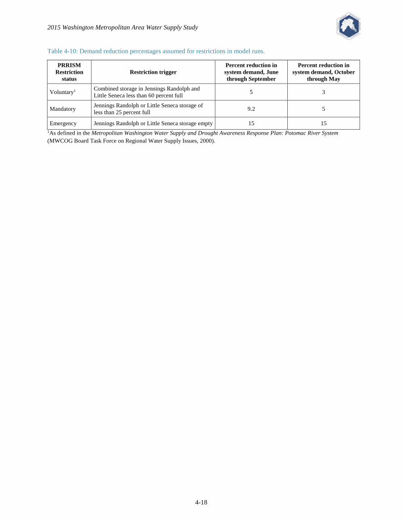
2015 Washington Metropolitan Area Water Supply Study
Table 4-10: Demand reduction percentages assumed for restrictions in model runs.
PRRISM Restriction
status Restriction trigger
Percent reduction in system demand, June through September
Percent reduction in system demand, October
through May
Voluntary1 Combined storage in Jennings Randolph and Little Seneca less than 60 percent full 5 3
Mandatory Jennings Randolph or Little Seneca storage of less than 25 percent full 9.2 5
Emergency Jennings Randolph or Little Seneca storage empty 15 15 1As defined in the Metropolitan Washington Water Supply and Drought Awareness Response Plan: Potomac River System (MWCOG Board Task Force on Regional Water Supply Issues, 2000).
4-18
2015 Washington Metropolitan Area Water Supply Study
5 Modeling System Resources & Operations in PRRISM
ICPRB’s planning model, PRRISM, is used in this study to evaluate the likelihood that the existing WMA water supply system could meet the demand forecasts presented in Chapter 3. The PRRISM model simulates the day-to-day operations of the system and the use of the Potomac River and system reservoirs during droughts to meet demands and the minimum flow-by target at Little Falls dam. This chapter provides details on PRRISM’s representation of system supplies, operations, and constraints.
The Potomac River supplies approximately three quarters of WMA system withdrawals. The remainder is provided by two “off-Potomac” reservoirs, Fairfax Water’s Occoquan Reservoir in the Occoquan watershed and WSSC’s Tridelphia and T. Howard Duckett reservoirs in the Patuxent watershed. The three CO-OP suppliers jointly fund storage in two reservoirs, Jennings Randolph and Little Seneca, located upstream of their Potomac River intakes, for augmentation of Potomac River flows during droughts. In addition, they fund a portion of the operations and maintenance costs of a third upstream reservoir, Savage, which is operated in conjunction with Jennings Randolph. The locations and storage capacities of system reservoirs are shown in Figure 1-1.
Changes are made to PRRISM on an ongoing basis to reflect recent changes in the system and improved knowledge resulting from new data and operational experience. The most significant changes since the last demand and availability forecast are:
• the use of a one-day Little Falls flow forecast to determine the Little Seneca Reservoir water supply release rate and Occoquan Reservoir withdrawal rate;
• a more detailed representation of the transfer of finished water between Fairfax Water’s eastern and western water service areas to improve simulation of load-shifts between Fairfax Water’s Potomac River and Occoquan Reservoir intakes;
• an update to the Patuxent water treatment plant’s minimum production rate from 27 MGD to 33 MGD to reflect recent plant upgrades, and use of a 20 MGD “emergency” Patuxent water treatment plant production rate to simulate intermittent use of the plant when Patuxent Reservoir storage falls below 1,000 MG;
• an update to the Jennings Randolph and Little Seneca reservoirs’ estimated sedimentation rates, based on recent hydrographic studies;
• the addition of Falls Church to the Fairfax Water system and simulation of the transfer of up to 35 MGD from Aqueduct to Fairfax Water;
• inclusion of Loudoun Water’s future water treatment plant and 1.02 BG raw water storage facility (Quarry A); and
• inclusion of the Town of Westernport’s additional withdrawal from Savage Reservoir.
Potomac River Flow
Flow in the Potomac River is usually ample and more than sufficient to meet water supply and environmental needs. Long-term average flow at the USGS stream gage at Little Falls dam (Station ID 01646500) is approximately 7,400 MGD, which is well above the 400 to 500 MGD typically withdrawn by the CO-OP suppliers. However, flow in the Potomac is highly variable and dependent on the time of year. Flows typically decrease during the summer and early fall due to higher evaporation rates in the
5-1

2015 Washington Metropolitan Area Water Supply Study
watershed and higher transpiration rates, that is, use of water by trees and other vegetation. The seasonal variation of flow in the Potomac River is apparent in Figure 5-1, which shows four daily statistics for historical “adjusted flow” values at Little Falls dam: minimum flow, 10th percentile flow, median flow, and 90th percentile flow. Adjusted flow at Little Falls dam is the flow that would have been observed in the absence of WMA withdrawals. The historical minimum flow, for example, 411 MGD on September 1, is the lowest adjusted flow that ever occurred on September 1 in the 84-year record of flow at the Little Falls gage (1930-2013). The median adjusted flow on September 1 of 1,855 MGD is the median of the 84 flow values that have occurred on September 1. From Figure 5-1 it is evident that on most days of the year WMA needs are still comfortably below the minimum flow ever recorded for that day. The graph also shows that flow in the Potomac River has at times been below the level necessary to meet today’s demands, especially in the months of August and September.
Figure 5-1: Adjusted daily flow at Little Falls dam in 2002, daily adjusted flow percentiles for 1930-2013 data, and drought year (2002) demands plus flow-by.
Figure 5-1 also shows WMA Potomac River demands in 2002, a recent drought year in which demands were high, plus the 100 MGD environmental flow-by at Little Falls dam. The graph of 2002 flows demonstrates the high variability in flows that can occur, even in drought years. The graph also shows that new minimum flow records were set 2002, notably in February, March and April.
The drought of record for the current WMA system occurred in 1930, when Potomac River flow was extremely low for an extended period of time, from mid-July through mid-December. The second most
100
1,0
00 1
0,00
0 1
00,0
00
Jan Feb Mar Apr May Jun Jul Aug Sep Oct Nov Dec
Adju
sted
Dai
ly F
low
at L
ittle
Fal
ls, M
GD
50th to 90th Percentile Flow 10th to 50th Percentile Flow
Historical Minimum to 10th Percentile Flow Zero to Historical Minimum Flow
Historical Minimum Flow
2002 WMA Potomac Demands plus Flow-by
2002 Adjusted Flow
5-2
2015 Washington Metropolitan Area Water Supply Study
serious drought in the basin occurred in the summer of 1966, when observed flow at Little Falls dropped to its lowest recorded level, 78 MGD.
PRRISM’s simulation of daily water availability is based on input time series of Potomac River natural flows, that is, estimates of flows that would have occurred without the effects of withdrawals, diversions, or reservoir regulations. Historical stream flow records have been used to develop “natural” daily Potomac River flows and reservoir inflows for input into PRRISM (Hagen and Steiner, 1998a; Hagen et al., 1998b; 1998c), during the period of record, October 1, 1929, through December 31, 2013. Thus, PRRISM can be used to evaluate whether the current system can meet forecasted demands under hydrologic conditions which occurred in each year of the 84-year historical record, including the drought years of 1930 and 1966. Results of this evaluation are given in Chapter 1. PRRISM is also used, as discussed in Chapter 7, to assess the vulnerability of the system to potential reductions in flow due to climate change.
5.1.1 Potomac Flow Recommendations
The current environmental flow recommendations for the Potomac River near Washington, D.C, are based on recommendations in a 1981 study conducted by the Maryland Department of Natural Resources (1981). This study was the result of a request by the USACE to the Maryland Department of Natural Resources to make a quantitative recommendation related to a clause in the LFAA on the “amount needed for flow in the Potomac River downstream from the Little Falls dam for the purpose of maintaining environmental conditions.” The study recommended a minimum daily environmental flow-by of 100 MGD at Little Falls dam. This number was subsequently incorporated into the LFAA emergency allocation. The study also contained a recommendation related to flow below Great Falls, which is located approximately nine miles above Little Falls dam. It recommended that when flow below Great Falls dropped below 500 MGD, Aqueduct begin shifting its withdrawal from its intake at Great Falls to its intake at Little Falls. This “load-shift” would have the effect of increasing flow between Great Falls and Little Falls dam by the amount of the shift. Because Aqueduct summer withdrawals at the time of the 1981 study were often near or at 200 MGD, this recommendation would have maintained flow between Great Falls and Little Falls dam at or near 300 MGD during low-flow periods.
A more recent study on the environmental needs of large rivers in the Potomac River basin, conducted by ICPRB, George Mason University, and the USGS for The Nature Conservancy (Cummins et al., 2010), reviewed these environmental flow recommendations. This study concluded that flow at Little Falls dam should be maintained above the 100 MGD flow-by and recommended that flow between Little Falls dam and Great Falls should be above 300 MGD, and that, as a precautionary measure until more ecological monitoring data is available to improve understanding of low-flow impacts, reservoir operating procedures should give consideration to maintaining variability during extreme low-flow periods.
CO-OP conducts drought operations with the goal of maintaining daily flow at Little Falls dam above the 100 MGD flow-by and flow between Great Falls and Little Falls dam above 300 MGD. As discussed below (Section 5.2.2.1), a substantial margin of safety of 130 MGD or greater is simulated in the current study for Little Seneca and Occoquan operations to help ensure that flow at Little Falls stays above 100 MGD.
5-3
2015 Washington Metropolitan Area Water Supply Study
Reservoir Operations
Jennings Randolph and Little Seneca reservoirs are both located upstream of the WMA water supply intakes and are used to augment flows in the Potomac River when the sum of predicted demands and the environmental flow-by at Little Falls dam is greater than forecasted Potomac River flow. Since the establishment of the CO-OP system and the completion of these reservoirs in the early 1980s, water supply releases from these reservoirs have only occurred during three periods of time: summer of 1999, summer of 2002, and fall of 2010.
The Patuxent and Occoquan reservoirs are used on a daily basis in conjunction with the Potomac River intakes to meet WSSC and Fairfax Water demands, respectively. The water withdrawn from these reservoirs reduces the amount of water that must be withdrawn from the Potomac. During periods of drought, the Patuxent and Occoquan reservoirs are operated based on CO-OP flow forecasts in coordination with Little Seneca Reservoir to maximize water supply reliability from a systems perspective.
All system reservoirs are operated in normal years with the goal that they have a 95 percent probability of being at least 90 percent full by June 1 of each year. This practice helps ensure that these reservoirs can be used to their maximum benefit under drought conditions. More details on these reservoir operations are given below.
5.2.1 North Branch Reservoirs
Jennings Randolph Reservoir and Savage Reservoir (the “North Branch reservoirs”) are located in the far northwestern corner of the Potomac River basin on the North Branch of the Potomac River (see Figure 1-1). These reservoirs are operated for four primary purposes: flood control, water quality enhancement, recreation, and water supply. Jennings Randolph is the system’s largest storage resource, with 13.1 BG of the reservoir’s conservation pool allocated to CO-OP water supply storage and the remaining 16.2 BG allocated to “water quality” storage. These two segments of storage are operated separately. The USACE’s Baltimore District Office manages this reservoir and makes releases from water quality storage continually to meet its primary objectives, and to the greatest degree possible, to provide whitewater boating and fishing opportunities downstream along with boating and beach access on Jennings Randolph Reservoir itself. Jennings Randolph water supply storage is only used at the request of CO-OP on behalf of the CO-OP suppliers. Savage Reservoir is operated in coordination with Jennings Randolph Reservoir, with releases generally made at a five-to-one ratio, but it does not have official storage allocations. Savage Reservoir also supplies water to the Town of Westernport, Maryland. The combined Jennings Randolph and Savage release is measured at the USGS stream gage (Station ID 01598500) at Luke, Maryland.
5.2.1.1 WMA Water Supply Releases
During periods of drought, CO-OP can request water supply releases from the North Branch reservoirs to augment flows in the Potomac River. CO-OP determines release rates based on forecasts of flow and demands. Because the North Branch reservoirs are located some 200 miles upstream of the WMA,
5-4

2015 Washington Metropolitan Area Water Supply Study
releases must be made approximately nine days in advance to allow for travel time downstream. To simulate the release decision, PRRISM uses an empirical equation for the recession of flow at Little Falls, derived from a data set of “natural” flows at Little Falls during historical periods of drought. Natural flow is defined as the flow that would have been observed at the USGS stream gage at Little Falls dam without the effects of WMA Potomac withdrawals and without the presence of the North Branch reservoirs. According to Equation (5-1), natural flow at Little Falls dam nine days in the future, Q Little Falls (t + 9), is related to natural flow at Little Falls dam on the current day, Q Little Falls (t), by the expression,
𝑄𝑄𝐿𝐿𝐿𝐿𝐿𝐿𝐿𝐿𝐿𝐿𝐿𝐿 𝐹𝐹𝐹𝐹𝐿𝐿𝐿𝐿𝐹𝐹(𝑡𝑡 + 9) = 289 𝑒𝑒(0.0009 𝑄𝑄𝐿𝐿𝐿𝐿𝐿𝐿𝐿𝐿𝐿𝐿𝐿𝐿 𝐹𝐹𝐹𝐹𝐿𝐿𝐿𝐿𝐹𝐹(𝐿𝐿)) (5-1)
where flow is measured in MGD and t represents time in days.
The Little Seneca Reservoir, less than a day's travel time from the WMA suppliers’ intakes, is used in conjunction with Jennings Randolph Reservoir so that releases made from the latter can be more conservative. No “margin of safety” is used to determine the Jennings Randolph Reservoir water supply release because if the release proves to be too small (because of lower than expected Potomac River flow or higher than expected demand), a release can be made from the smaller, closer Little Seneca Reservoir to make up for any temporary shortfalls that become apparent as water from Jennings Randolph Reservoir travels to the intakes. These operations are incorporated into PRRISM’s decision rules.
5.2.1.2 Operation of the North Branch Reservoirs
Management objectives for the North Branch reservoirs have been developed by the USACE’s Baltimore District Office in accordance with the reservoirs’ master manuals of operations and with input from the North Branch Potomac River Advisory Committee. This committee was established in 2005 to provide a stakeholder forum regarding operations and management of the reservoirs, the surrounding public lands, and downstream flow levels (NPS, 2008). The USACE management goals have evolved over the years as water quality conditions in the North Branch have changed. Prior to the 1980s, the North Branch Potomac River had serious pH problems due to acid mine drainage. Water quality releases from Jennings Randolph Reservoir and concurrent releases of higher quality water from Savage Reservoir were made to improve downstream pH conditions during low-flow periods in the summer and early fall. But by the late 1980s, acid mine remediation efforts had alleviated these water quality problems, and viable fisheries developed in Jennings Randolph Reservoir and in downstream reaches of the North Branch. Other water quality issues have come to the forefront, such as control of temperature to support cold-water trout populations. At the same time, recreational activities on and below the reservoirs have increased and gained in prominence, especially fishing and whitewater boating. Because of the changing conditions, CO-OP has spent a substantial amount of effort working with the reservoir operators and stakeholders to study how operations can be changed in order to better balance needs within the Potomac River basin. The USACE has gradually adjusted its operations to reflect these changes but it is possible that more can be done in future years.
The representation of Jennings Randolph Reservoir water quality releases in the current version of PRRISM, developed in close coordination with the USACE’s Baltimore District Office, is described in detail in Ahmed et al. (2010). PRRISM simulates all recreational and environmental storage elevation targets that are either mandated by the government or recommended by the North Branch Potomac River
5-5

2015 Washington Metropolitan Area Water Supply Study
Advisory Committee. PRRISM simulates the USACE’s balancing of competing needs for the limited water resource, including a stepped rule table to guide releases when downstream flow and reservoir elevation targets need to be abandoned during dry conditions.
PRRISM also simulates operation of Savage Reservoir according to rule curves, with adjustments of releases to accommodate the needs of downstream fisheries. Matched releases from Savage Reservoir concurrent with Jennings Randolph Reservoir water supply releases are also simulated. During the drawdown season (approximately late spring through early fall), Jennings Randolph Reservoir water supply releases are matched by Savage Reservoir releases at a five-to-one ratio. Thus, 84 percent of total flow augmentation needed for WMA water supply comes from Jennings Randolph Reservoir water supply storage and 16 percent comes from Savage Reservoir. The original need for the Savage Reservoir matched release is described in Savage Reservoir Operation and Maintenance Cost Sharing Agreement, signed in 1982 by the CO-OP suppliers, the UPRC, and Allegany County. The agreement states that the matched releases from Savage Reservoir were originally necessary to dilute the acidic water released from Jennings Randolph Reservoir water supply storage; and thereby reduce the acidity of water released from Jennings Randolph Reservoir during periods of extreme low-flow. Now that acid mine drainage has substantially subsided in the North Branch of the Potomac, matched releases from Savage Reservoir no longer serve their intended purposes. However, during the drought of 2002 Savage Reservoir was used to match the Jennings Randolph Reservoir water supply release even though water acidity was not a concern. The continuing implementation of this agreement is contingent on approval by the UPRC, the owners of Savage Reservoir. These matches are discontinued if Savage Reservoir drops below a guide curve from the Baltimore District Office’s Master Manual (Curve C, which is meant to protect the Town of Westernport’s water supply).
PRRISM’s simulation of the Town of Westernport’s withdrawal has increased by 2.2 MGD (annual average for industrial use) from its original assumption of 1 MGD (for municipal water supply) for a total withdrawal of 3.2 MGD. A recent permit from the Maryland Department of the Environment granted the Town of Westernport permission to increase its withdrawal from Savage Reservoir in order to supply water to the NewPage paper mill in Luke, Maryland, for use in a specific manufacturing process. NewPage previously withdrew water for this process directly from the North Branch Potomac River from its intake located just downstream of the USGS stream gage (Station ID 01598500) at Luke, Maryland, but prefers water from Savage Reservoir because its higher quality reduces operational costs. Wastewater from the NewPage plant is processed by the Westernport wastewater treatment plant, whose discharge point is downstream of both the USGS stream gage at Luke and the NewPage intake.
The increased withdrawal permit includes a set of triggers developed by CO-OP to predict major droughts. The trigger thresholds and associated withdrawal limits were designed to minimize depletion of Savage Reservoir storage while allowing the Town of Westernport to withdraw the full permitted amount as often as possible. The dates and trigger thresholds are shown in Table 5-1.
5-6
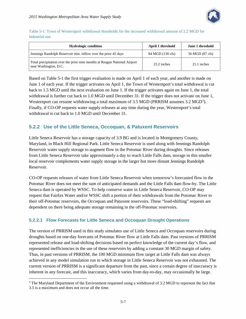
2015 Washington Metropolitan Area Water Supply Study
Table 5-1: Town of Westernport withdrawal thresholds for the increased withdrawal amount of 2.2 MGD for industrial use.
Hydrologic condition April 1 threshold June 1 threshold
Jennings Randolph Reservoir min. inflow over the prior 45 days 84 MGD (130 cfs) 56 MGD (87 cfs)
Total precipitation over the prior nine months at Reagan National Airport near Washington, D.C. 23.2 inches 21.1 inches
Based on Table 5-1 the first trigger evaluation is made on April 1 of each year, and another is made on June 1 of each year. If the trigger activates on April 1, the Town of Westernport’s total withdrawal is cut back to 1.5 MGD until the next evaluation on June 1. If the trigger activates again on June 1, the total withdrawal is further cut back to 1.0 MGD until December 31. If the trigger does not activate on June 1, Westernport can resume withdrawing a total maximum of 3.5 MGD (PRRISM assumes 3.2 MGD3). Finally, if CO-OP requests water supply releases at any time during the year, Westernport’s total withdrawal is cut back to 1.0 MGD until December 31.
5.2.2 Use of the Little Seneca, Occoquan, & Patuxent Reservoirs
Little Seneca Reservoir has a storage capacity of 3.9 BG and is located in Montgomery County, Maryland, in Black Hill Regional Park. Little Seneca Reservoir is used along with Jennings Randolph Reservoir water supply storage to augment flow in the Potomac River during droughts. Since releases from Little Seneca Reservoir take approximately a day to reach Little Falls dam, storage in this smaller local reservoir complements water supply storage in the larger but more distant Jennings Randolph Reservoir.
CO-OP requests releases of water from Little Seneca Reservoir when tomorrow’s forecasted flow in the Potomac River does not meet the sum of anticipated demands and the Little Falls dam flow-by. The Little Seneca dam is operated by WSSC. To help conserve water in Little Seneca Reservoir, CO-OP may request that Fairfax Water and/or WSSC shift a portion of their withdrawals from the Potomac River to their off-Potomac reservoirs, the Occoquan and Patuxent reservoirs. These “load-shifting” requests are dependent on there being adequate storage remaining in the off-Potomac reservoirs.
5.2.2.1 Flow Forecasts for Little Seneca and Occoquan Drought Operations
The version of PRRISM used in this study simulates use of Little Seneca and Occoquan reservoirs during droughts based on one-day forecasts of Potomac River flow at Little Falls dam. Past versions of PRRISM represented release and load-shifting decisions based on perfect knowledge of the current day’s flow, and represented inefficiencies in the use of these reservoirs by adding a constant 30 MGD margin of safety. Thus, in past versions of PRRISM, the 100 MGD minimum flow target at Little Falls dam was always achieved in any model simulation run in which storage in Little Seneca Reservoir was not exhausted. The current version of PRRISM is a significant departure from the past, since a certain degree of inaccuracy is inherent in any forecast, and this inaccuracy, which varies from day-to-day, may occasionally be large.
3 The Maryland Department of the Environment requested using a withdrawal of 3.2 MGD to represent the fact that 3.5 is a maximum and does not occur all the time.
5-7

2015 Washington Metropolitan Area Water Supply Study
Imperfect knowledge of tomorrow’s flow may result in operational decisions that fail to achieve the Little Falls flow-by. To reduce the probability of this event, margins of safety for Little Seneca Reservoir and Occoquan Reservoir operations have been increased in the new version of PRRISM from 30 MGD to 130 MGD, and higher under certain conditions. This more detailed incorporation into PRRISM of varying flow forecast accuracies provides a more realistic representation of actual CO-OP operations during past droughts. Of course, as flow forecast tools improve in the future, forecast inaccuracies may be reduced. CO-OP is currently testing a new tool which provides flow forecasts based on real-time meteorological data and forecasts from the National Weather Service and flow predictions from a version of the Chesapeake Bay Program’s watershed model.
A one-day flow forecast was determined to be most appropriate for simulation of both Little Seneca Reservoir and Occoquan Reservoir operational decisions based on CO-OP experience during recent droughts and drought exercises. Time of travel experiments and observations indicate that under very low flow conditions it takes a little over a day for a release from Little Seneca Reservoir to be observed at the USGS stream gage at Little Falls, and changes in withdrawal rates at Fairfax Water’s Potomac River intake take approximately 15 hours to be observed at this gage. In addition, Fairfax Water currently requires up to a full day to shift a portion of its withdrawals from the Potomac River to the Occoquan Reservoir, though in the future these times may be reduced. Since a daily time step is used in PRRISM simulations, a one-day lag time was chosen to simulate the impact of these operations at Little Falls, consistent with a one-day flow forecast for operational decisions.
The one-day flow forecast implemented in PRRISM is similar to the forecast currently used in CO-OP’s drought operations spreadsheet tools. It is based on upstream gage data from the USGS’s stream gage on the Potomac River at Point of Rocks, Maryland (Station ID 01638500), and also data from the watersheds of tributaries that discharge into the Potomac River between Point of Rocks and Little Falls dam. The flow prediction assumes that flow at Little Falls dam (“LF”) is approximately the sum of flow at Point of Rocks (“POR”) and flow from the tributary (“tribs”) watersheds, with appropriate lag times, ρ1 and ρ2 , that is,
Q LF (t) ≅ Q POR (t - ρ1) + Q tribs (t - ρ2) (5-2)
Flow at Little Falls dam tomorrow is flow today plus the change in flow over the course of one day, that is,
Q LF (t + 1) = Q LF (t) + [Q LF (t + 1) - Q LF (t)] (5-3)
The change in flow can be approximated by the sum of upstream flows given by Equation (5-2), giving
Q LF (t + 1) ≅ Q LF (t) + [Q POR (t + 1 - ρ1) - Q POR (t - ρ1) + Q tribs (t + 1 - ρ2) - Q tribs (t - ρ2)] (5-4)
In Equation (5-2) the lag times for the tributary flow contributions have been approximated by a single value, since these contributions are generally small compared to flow in the Potomac River at Point of Rocks and since these lags cannot be readily determined with the available data.
An evaluation of the low-flow prediction performance of the one-day forecast model, Equation (5-4), was made using PRRISM inputs of historical daily time series data for Point of Rocks, Little Falls dam, and tributaries from October 1, 1929, through December 31, 2013. In the current version of PRRISM, the
5-8

2015 Washington Metropolitan Area Water Supply Study
low-flow lag times, ρ1 and ρ2 , are both set at 2.4 days. This value provides the best model performance and is consistent with CO-OP’s experience during low-flow periods. Statistics for low-flow model errors are given in Table 5-2, where low-flow errors are defined as errors on days when flow at Little Falls dam is less than 700 MGD.
Table 5-2: Statistics for low-flow model errors at Little Falls dam (MGD).
Mean low-flow error
Mean low-flow absolute
error
Maximum low-flow
error
Minimum low-flow
error
1st percentile low-flow
error
5th percentile low-flow
error
Low-flow error
standard deviation
Low-flow coefficient of correlation
-3 41 515 -528 -244 -98 72 0.40
Graphs comparing the forecast and actual data for historical flows from the droughts of 1930 and 1966 are shown in Figure 5-2 and Figure 5-3, respectively. The graph indicates that Equation (5-4) does a reasonable job of predicting flows during these extreme low-flow periods. However, prediction errors can sometimes be significant, especially on days near the arrival of a small storm peak. This is due to the limitation of the constant time of travel approximation; higher flow portions of the hydrograph travel at faster velocities than lower flow portions.
Figure 5-2: Comparing the forecast and actual data for historical Little Falls flows from the drought of 1930.
5-9
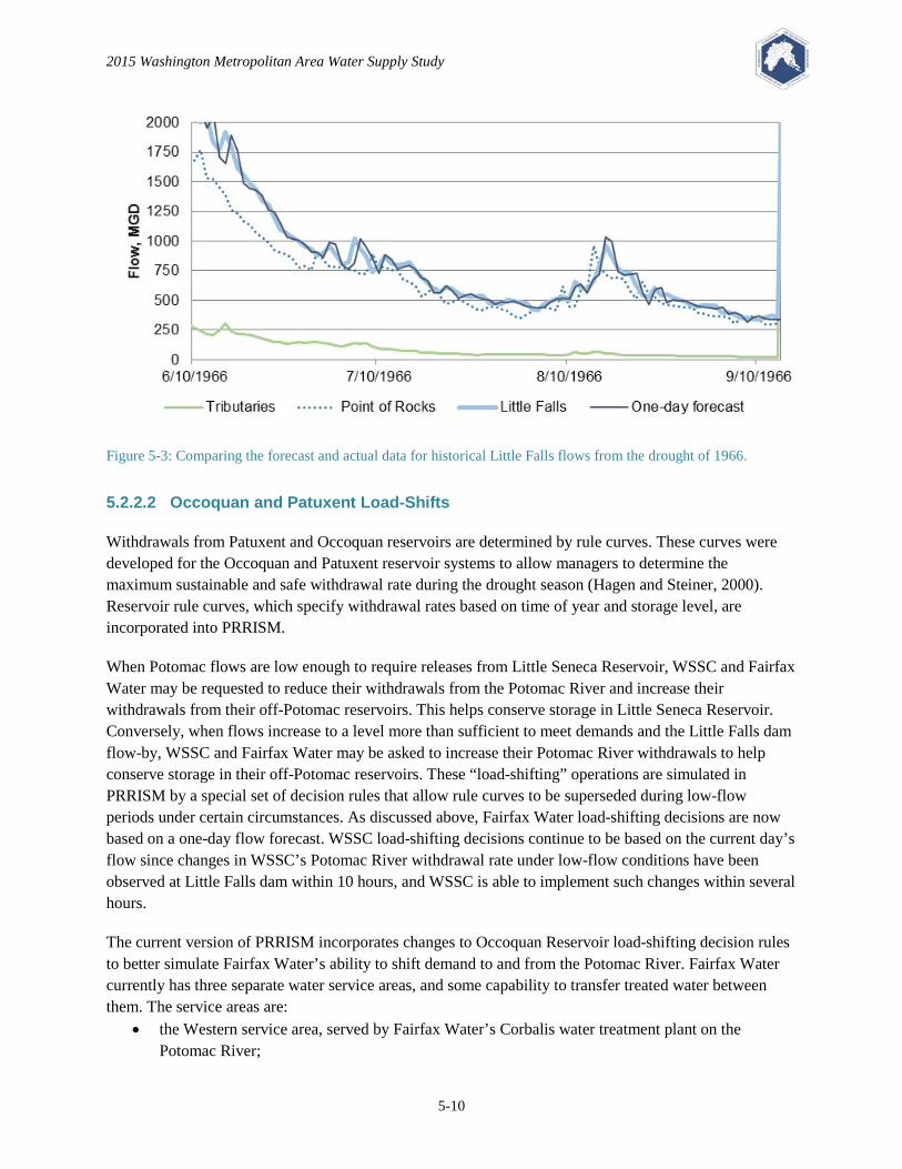
2015 Washington Metropolitan Area Water Supply Study
Figure 5-3: Comparing the forecast and actual data for historical Little Falls flows from the drought of 1966.
5.2.2.2 Occoquan and Patuxent Load-Shifts
Withdrawals from Patuxent and Occoquan reservoirs are determined by rule curves. These curves were developed for the Occoquan and Patuxent reservoir systems to allow managers to determine the maximum sustainable and safe withdrawal rate during the drought season (Hagen and Steiner, 2000). Reservoir rule curves, which specify withdrawal rates based on time of year and storage level, are incorporated into PRRISM.
When Potomac flows are low enough to require releases from Little Seneca Reservoir, WSSC and Fairfax Water may be requested to reduce their withdrawals from the Potomac River and increase their withdrawals from their off-Potomac reservoirs. This helps conserve storage in Little Seneca Reservoir. Conversely, when flows increase to a level more than sufficient to meet demands and the Little Falls dam flow-by, WSSC and Fairfax Water may be asked to increase their Potomac River withdrawals to help conserve storage in their off-Potomac reservoirs. These “load-shifting” operations are simulated in PRRISM by a special set of decision rules that allow rule curves to be superseded during low-flow periods under certain circumstances. As discussed above, Fairfax Water load-shifting decisions are now based on a one-day flow forecast. WSSC load-shifting decisions continue to be based on the current day’s flow since changes in WSSC’s Potomac River withdrawal rate under low-flow conditions have been observed at Little Falls dam within 10 hours, and WSSC is able to implement such changes within several hours.
The current version of PRRISM incorporates changes to Occoquan Reservoir load-shifting decision rules to better simulate Fairfax Water’s ability to shift demand to and from the Potomac River. Fairfax Water currently has three separate water service areas, and some capability to transfer treated water between them. The service areas are:
• the Western service area, served by Fairfax Water’s Corbalis water treatment plant on the Potomac River;
5-10
2015 Washington Metropolitan Area Water Supply Study
• the Eastern service area, served by Fairfax Water’s Griffith water treatment plant on Occoquan Reservoir; and
• the Central service area, consisting of the City of Falls Church, and served by water purchased from Aqueduct.
The breakdown of demands in the three smaller service areas is given in Table 5-3.
Table 5-3: Percent of total demand estimated for each Fairfax Water service area (Gregory Prelewicz, personal communication, January 13, 2015).
Fairfax Water service areas Percent of forecasted annual 2040 demand
Western 44.34
Central 10.51
Eastern 45.05
Total 100.00 Note: Loudoun Water demands are provided 100 percent by the Potomac River (Western service area) and add approximately 12.0 MGD to Fairfax Water’s Western service area estimate assuming that in 2040 an annual average of 20 MGD is provided by the Loudoun Water water treatment plant.
Treated water can be transferred from the Western service area to the Eastern service area at a maximum rate of 65 MGD. Changes in this transfer rate can be made quickly via remote adjustments of valves. Treated water can be transferred from the Eastern service area to the Western service area at a maximum rate of 35 MGD. Changes in this transfer rate are currently limited to 10 MGD per day and require up to a day of advance warning, since a manual adjustment of valves is required. PRRISM has been updated to better reflect the speed with which Fairfax Water can implement a transfer depending on the direction.
Effects of Sedimentation on Reservoir Storage
Reservoir storage capacities tend to decrease with time due to the deposition of sediment. Reservoir sedimentation rates are highly variable and dependent on hydrologic conditions, with the majority of sediment deposition occurring during very large storm events. New estimates of reservoir storage capacities and sediment depositions are available for several WMA reservoirs, based on recent bathymetric surveys. The decrease in storage capacity in the WMA water supply system, as a function of forecast year, is represented in PRRISM by means of an assumed sedimentation rate for each reservoir. Table 5-4 shows the estimated current and projected reservoir storage for the system reservoirs, along with sedimentation rates assumed in the current study. Some of the sedimentation rates in Table 5-4 are significantly less than the rates assumed in Part 1 of the 2010 demand study (Ahmed et al., 2010), resulting in higher estimates of future system storage capacity. A discussion of new data follows.
5-11

2015 Washington Metropolitan Area Water Supply Study
Table 5-4: Effects of sedimentation on reservoir storage capacities.
Reservoir Baseline year
Usable capacity in baseline year
(MG)
Usable capacity in year 2015
(MG)
Usable capacity in year 2040
(MG)
Rate of sedimentation
assumed (MG/yr)
Occoquan Reservoir1 2010 8.05 7,950 7,450 20
Patuxent reservoirs2 2004 10,320 10,176 9,708 17
Little Seneca Reservoir3 2010 3,903 3,883 3,783 4
Jennings Randolph Reservoir - water supply4 2013 13,098 13,057 12,556 45 (distributed
between water supply and quality
storages) Jennings Randolph Reservoir - water quality4 2013 16,295 16,246 15,622
Savage Reservoir5 2005 6,241 6,061 5,611 18 1 Baseline usable capacity and sedimentation rate from Fairfax Water (Greg Prelewicz, personal communication, March 18, 2014). 2 Baseline usable capacity and sedimentation rate from Ortt, et al. (2007). 3 Baseline usable capacity and sedimentation rate from Ortt, el al. (2011). 4 Baseline usable capacity based on the 2013 revised stage-storage curve provided by Bill Haines (personal communication, January 16, 2014). 5 Baseline usable capacity and sedimentation rate from Kame’enui et al. (2005).
5.3.1 Occoquan Reservoir
Reviews of past bathymetric surveys and sedimentation rate estimates are available in a report prepared for Fairfax Water by CDM (2002). Fairfax Water provided ICPRB with results from the most recent bathymetric survey, conducted in 2010. The 2010 survey found that the volume of the reservoir at full pool elevation, 122 feet above mean sea level (MSL), was 8.33 BG. This volume is larger than the volume computed in a survey conducted in 2000, which was 8.313 BG. A portion of the storage capacity, 0.28 BG, is located below the elevation of the invert of the lowest intake, 80 feet. Thus, the estimate of useable storage in 2010 is 8.05 BG.
Fairfax Water suggested that for planning purposes, the “low” value of the Occoquan Reservoir sedimentation rate estimated in past studies, 20 MG/yr, be used to account for potential future fluctuations in sedimentation. Recent CO-OP studies have assumed a sedimentation rate of 40 MG/yr, computed from the volume lost from 1995 to 2000, determined from detailed bathymetric surveys by the Occoquan Water Monitoring Laboratory (CDM, 2002).
5.3.2 Patuxent Reservoirs
The most recent estimates of volumes and sedimentation rates for WSSC’s Patuxent reservoirs, Tridelphia and T. Howard Duckett, are available from a study by the Maryland Geological Survey (MGS) for the Maryland Department of Natural Resources (Ortt et al., 2007). Bathymetric data was collected in May and June of 2004 for Tridelphia and in April and August of 2005 for T. Howard Duckett. Estimated total volume of Tridelphia at mean pool level (366.4 feet above MSL) was 6.66 BG. Estimated total volume of T. Howard Duckettat mean pool level (286.4 feet above MSL) was 5.54 BG. Thus, the estimated total
5-12
2015 Washington Metropolitan Area Water Supply Study
volume of the two reservoirs in 2004 was 12.2 BG. Subtracting an adjustment of 1.48 BG for the volume between mean pool level and normal pool level, and an adjustment of 0.4 BG for T. Howard Duckettdead storage, the resulting estimate for usable storage in the two reservoirs in 2004 is 10.32 BG.
The MGS observed from available data “a distinct pattern of mixed sediment erosion and deposition.” They estimated a combined net sedimentation rate for the two reservoirs of 17 MG/yr. This is based on a rate calculated from the loss of storage volume between 1942 and 2004 in Tridelphia Reservoir and the loss between 1954 and 2005 in T. Howard DuckettReservoir. A somewhat higher sedimentation rate of 24 MG/yr, used in previous ICPRB studies, was based on loss estimates from a 1995-1996 survey conducted by Ocean Services, Inc. (Ortt et al., 2007).
5.3.3 Little Seneca Reservoir
Updated information on the sedimentation rate of Little Seneca Reservoir is available in a recent study by the MGS for the Maryland Department of Natural Resources (Ortt et al., 2011). New bathymetric data for the reservoir was collected in July and August of 2010. These data indicated a total storage capacity of 3.922 BG at mean pool level (385 feet above MSL). This volume can be compared to a previous analysis of the pre-construction topography from 1979 and also to the bathymetric survey conducted by Ocean Surveys, Inc., in 1996, which indicated a storage capacity of 3.86 BG. According to the MGS, the fact that the current capacity of the reservoir is more than the calculated capacity from the 1996 survey is likely due to the greater density of data in the 2010 survey. The sedimentation rate calculated from the pre-construction topography and the 2010 bathymetry is 4 MG/yr.
5.3.4 Jennings Randolph Reservoir
The original “design” sedimentation rate for Jennings Randolph Reservoir was 20.65 acre-feet per year (ac-ft/year), or 6.7 MG/yr. This rate was estimated from suspended sediment concentrations measured in water samples from the North Branch Potomac River at Kitzmiller (Burns and McArthur, 1996). Since the completion of the reservoir, the USACE’s Baltimore District Office has conducted surveys to monitor sediment accumulation in Jennings Randolph Reservoir and to estimate changes in its capacity, as summarized in Table 5-5.
The original design sedimentation rate was used to reduce the reservoir storage capacity determined from the 1964 topographic survey, which was the first survey that took place before the completion of the dam in May 1981. Impoundment of water in the reservoir began in July 1981, and water in the reservoir reached the conservation pool level, at 1,466 feet, in May 1982. From the pre-impoundment survey, the original capacity of the reservoir conservation pool was estimated to be 94,707 ac-ft (30,860 MG), with a usable capacity (above the lowest gate sill) of 94,398 ac-ft (30,760 MG). The USACE gave the storage capacity of the reservoir as 92,000 ac-ft (29,978 MG), after subtracting an estimated 2,707 ac-ft to account for unusable storage and anticipated sediment accumulation over a 100-year period (USACE, 1986). According to the agreed upon percentage of storage in the reservoir allocated to water supply, 44.56 percent, and to water quality, 55.44 percent, the water supply and water quality storage capacities were 40,995 ac-ft (13,358 MG) and 51,005 ac-ft (16,620 MG), respectively.
5-13
2015 Washington Metropolitan Area Water Supply Study
Data from a new hydrologic survey conducted by Bowen Engineering and Surveying in April 2013 suggests a Jennings Randolph Reservoir sedimentation rate equal to 138 ac-ft/yr (45 MG/yr). This 2013 hydrographic data was merged with topographic (above water) mapping prepared in 1998 by Horizons, Inc. from a 1997-1998 survey to produce an updated composite data set (Bill Haines, personal communication, January 16, 2014). This survey resulted in a second revision of the elevation-area-capacity tables (dated December 2013) for the reservoir. Results indicated a total capacity of the reservoir conservation pool as 90,313 ac-ft (29,429 MG), and the usable capacity (above the lowest gate sill) is 90,203 ac-ft (29,393 MG). This results in a usable storage capacity of 40,194 ac-ft (13,097 MG) for water supply and 50,009 ac-ft (16,295 MG) for water quality. This equals a 4.6 percent loss (4,394 ac-ft, or 1,432 MG) in storage between impoundment of the reservoir in July 1981 and the completion of the hydrographic survey in April 2013. This also equals a 2.5 percent gain (2,087 ac-ft, 680 mg) in storage between the 1997-1998 survey and the 2013 survey.
The 2013 sedimentation rate was significantly less than the 1997-1998 estimate. A possible reason is that the 2013 hydrographic survey was done using different equipment and techniques from those used in earlier surveys (Bill Haines, personal communication, January 16, 2014). The 1997-1998 and 2013 survey had very different data densities. In 1997 TVGA Engineering used 60 transects spaced roughly 500-750 feet apart, where in 2013 Bowen Engineering & Surveying used about 175 transects spaced roughly 200-250 feet apart. Another difference is that the “frustum of a circular cone formula” or conical formula was used in 2013 instead of the average end area formula used in the 1997-1998 survey.
Available survey results for total conservation pool storage capacity are summarized in Table 5-5 and plotted in Figure 5-4. The current study assumed a sedimentation rate of 45 MG/yr taken from the simple slope calculation for the July 1981 and the April 2013 conservation pool volumes at an elevation of 1,466 feet. In contrast, the 2010 demand study assumed a sedimentation rate of 127 MG/yr estimated using a Sen’s nonparametric estimate for slope calculated from the median value of slopes computed from all possible pairs of data points (Gilbert, 1987). Using the 45 MG/yr rate along with the USACE’s estimated capacity in 2013, the best estimate for Jennings Randolph conservation pool storage capacity in the year 2015 is approximately 29.3 BG, with 13.1 BG allocated to water supply and 16.2 BG allocated to water quality (Table 5-5), reflecting a loss of storage capacity of 4.8 percent since 1981. By 2040, the storage capacity loss is projected to be 7.2 percent.
The 2013 hydrologic survey culminated in a letter from the USACE that formalized the redistribution of the water supply and water quality storage accounts in Jennings Randolph Reservoir through a revised Exhibit A (USACE, 2014). Both the initial and future water storage agreements contain clauses that address potential future changes in reservoir storage space due to sedimentation. These clauses state that whenever necessary, there shall be an equitable redistribution of storage space among purposes served by the project including municipal and industrial water supply. The revised Exhibit A contains a table displaying storage capacities associated with various reservoir elevations and project purposes, which are reflected in the text above, Table 5-5, and Figure 5-4.
5-14
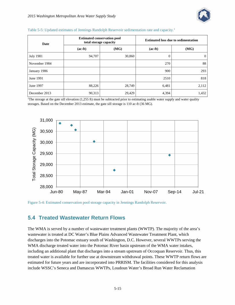
2015 Washington Metropolitan Area Water Supply Study
Table 5-5: Updated estimates of Jennings Randolph Reservoir sedimentation rate and capacity.1
Date Estimated conservation pool
total storage capacity Estimated loss due to sedimentation
(ac-ft) (MG) (ac-ft) (MG)
July 1981 94,707 30,860 0 0
November 1984 270 88
January 1986 900 293
June 1991 2510 818
June 1997 88,226 28,749 6,481 2,112
December 2013 90,313 29,429 4,394 1,432 1The storage at the gate sill elevation (1,255 ft) must be subtracted prior to estimating usable water supply and water quality storages. Based on the December 2013 estimate, the gate sill storage is 110 ac-ft (36 MG).
Figure 5-4: Estimated conservation pool storage capacity in Jennings Randolph Reservoir.
Treated Wastewater Return Flows
The WMA is served by a number of wastewater treatment plants (WWTP). The majority of the area’s wastewater is treated at DC Water’s Blue Plains Advanced Wastewater Treatment Plant, which discharges into the Potomac estuary south of Washington, D.C. However, several WWTPs serving the WMA discharge treated water into the Potomac River basin upstream of the WMA water intakes, including an additional plant that discharges into a stream upstream of Occoquan Reservoir. Thus, this treated water is available for further use at downstream withdrawal points. These WWTP return flows are estimated for future years and are incorporated into PRRISM. The facilities considered for this analysis include WSSC’s Seneca and Damascus WWTPs, Loudoun Water’s Broad Run Water Reclamation
28,000
28,500
29,000
29,500
30,000
30,500
31,000
Jun-80 May-87 Mar-94 Jan-01 Nov-07 Sep-14 Jul-21
Tota
l Sto
rage
Cap
acity
(MG
)
5-15
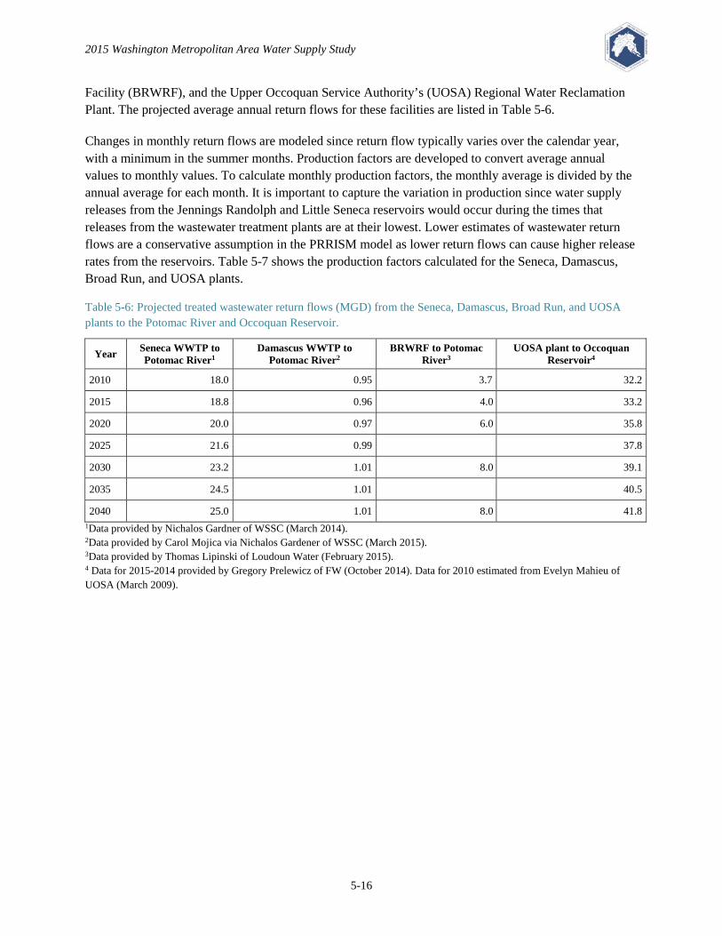
2015 Washington Metropolitan Area Water Supply Study
Facility (BRWRF), and the Upper Occoquan Service Authority’s (UOSA) Regional Water Reclamation Plant. The projected average annual return flows for these facilities are listed in Table 5-6.
Changes in monthly return flows are modeled since return flow typically varies over the calendar year, with a minimum in the summer months. Production factors are developed to convert average annual values to monthly values. To calculate monthly production factors, the monthly average is divided by the annual average for each month. It is important to capture the variation in production since water supply releases from the Jennings Randolph and Little Seneca reservoirs would occur during the times that releases from the wastewater treatment plants are at their lowest. Lower estimates of wastewater return flows are a conservative assumption in the PRRISM model as lower return flows can cause higher release rates from the reservoirs. Table 5-7 shows the production factors calculated for the Seneca, Damascus, Broad Run, and UOSA plants.
Table 5-6: Projected treated wastewater return flows (MGD) from the Seneca, Damascus, Broad Run, and UOSA plants to the Potomac River and Occoquan Reservoir.
Year Seneca WWTP to Potomac River1
Damascus WWTP to Potomac River2
BRWRF to Potomac River3
UOSA plant to Occoquan Reservoir4
2010 18.0 0.95 3.7 32.2
2015 18.8 0.96 4.0 33.2
2020 20.0 0.97 6.0 35.8
2025 21.6 0.99 37.8
2030 23.2 1.01 8.0 39.1
2035 24.5 1.01 40.5
2040 25.0 1.01 8.0 41.8 1Data provided by Nichalos Gardner of WSSC (March 2014). 2Data provided by Carol Mojica via Nichalos Gardener of WSSC (March 2015). 3Data provided by Thomas Lipinski of Loudoun Water (February 2015). 4 Data for 2015-2014 provided by Gregory Prelewicz of FW (October 2014). Data for 2010 estimated from Evelyn Mahieu of UOSA (March 2009).
5-16

2015 Washington Metropolitan Area Water Supply Study
Table 5-7: Production factors (MGD) for treated wastewater return flows for Seneca, Damascus, Broad Run, and UOSA plants.
Month Seneca WWTP (minimum of 2010-2013)1
Damascus WWTP (minimum of 2010-2014)2
BRWRF (minimum of 2010-2014)3
UOSA plant (minimum of 2010-2014)4
January 0.97 0.84 0.95 0.87
February 0.99 0.97 0.98 0.99
March 1.01 1.06 1.01 1.02
April 0.97 0.95 0.91 0.91
May 0.99 0.94 0.99 0.95
June 0.94 0.84 0.95 0.91
July 0.92 0.78 0.83 0.87
August 0.93 0.79 0.81 0.88
September 0.92 0.77 0.86 0.85
October 0.97 0.78 0.94 0.88
November 0.97 0.82 0.96 0.89
December 0.97 0.90 0.91 0.94 1Data provided by Nichalos Gardener of WSSC (March 2014). 2Data provided by Carol Mojica via Nichalos Gardener of WSSC (March 2015). 3Data provided by Thomas Lipinski of Loudoun Water (February 2015). 4Data provided by Gregory Prelewicz via Brian Owsenek of UOSA (March 2015).
Production Losses
New estimates of water losses from the raw water treatment process are incorporated into this study. In previous CO-OP studies, losses were only assumed to occur at Fairfax Water’s Griffith water treatment plant. Assumed water treatment plant losses used in the current study are compared with values used in the 2010 study (Ahmed et al., 2010) in Table 5-8.
Historically, residual solid material associated with water treatment processes, which includes sediment contained in the raw water and solids from treatment process coagulants, were typically discharged back into the source water. Because the residual material also contained water, this discharge resulted in negligible net water loss from the finished water treatment process. Water quality concerns have led to restrictions on discharges from water treatment plants and requirements that residual solids be dewatered and transported to off-site locations. In 1996, WSSC entered into an agreement with the Maryland Department of the Environment to build facilities to remove solids from its Potomac water treatment plant discharge, with an exception for periods of high Potomac River flow (Montgomery County, 2002). To satisfy new U.S. Environmental Protection Agency permit requirements, Aqueduct completed a new residuals management facility in November 2012 (USACE’s Baltimore District Office website: http://www.nab.usace.army.mil/Missions/WashingtonAqueduct/OngoingProjectsStudies.aspx, accessed February 1, 2015). Fairfax Water’s Griffith water treatment plant at the Occoquan Reservoir and its Corbalis water treatment plant on the Potomac River are relatively new, and both have residual solids
5-17

2015 Washington Metropolitan Area Water Supply Study
management facilities. In 2012, a change occurred in the Corbalis plant’s solids processing (Greg Prelewicz, personal communication, March 18, 2014). Water removed from the plant’s belt filter solids processing facilities was now sent through an on-site stormwater pond to discharge through a Virginia Pollutant Discharge Elimination System permitted outfall to a nearby tributary of Sugarland Run. Prior to 2012, this water, typically less than two to three percent of total production, was re-cycled to the head of the plant.
Table 5-8: Assumed production losses for CO-OP system water treatment plants used in PRRISM.
Study Year FW – Griffith FW – Corbalis WSSC – Potomac WSSC – Patuxent Aqueduct
2010 12% 0% 0% 0% 0%
2015 10% 3% 3% 3% 3%
Aqueduct provided daily withdrawal and production estimates for the period 2004-2013. Withdrawal estimates for both Little Falls and the total system are made hourly by system operators. System total withdrawal is the sum of flows from Dalecarlia Reservoir to the McMillan water treatment plant, which is measured with a Venturi meter and is fairly accurate, and to the Dalecarlia water treatment plant, which is measured with a meter thought to be less accurate. Production is the sum of flows to Arlington, Falls Church, and the District of Columbia. These production flows are measured by Venturi meters which are calibrated monthly (Alex Gorzalski, personal communication, March 7, 2014). Based on these data, Aqueduct’s average production loss is three percent. There was significant variation with season, with an average summer (June, July, August, September) loss of two percent and an average winter (December, January, February) loss of six percent.
WSSC provided daily data on production, raw water withdrawals, and net withdrawals from both their Potomac River and Patuxent reservoir intakes and water treatment plants (Nichalos Gardner, personal communication, March 11, 2014; June 20, 2014). Net withdrawals take into account water reclaimed and returned either to the finished water treatment process or to the source. Defining treatment loss as the difference between raw water withdrawal and water production, average treatment process losses for the period 2009-2013 were calculated to be three percent and five percent for the Potomac and Patuxent water treatment plants, respectively. Both winter and summer losses were three percent and four percent for the Potomac and Patuxent plants, respectively.
Fairfax Water provided forecasted production loss rates for the Griffith water treatment plant at the Occoquan Reservoir and the Corbalis water treatment plant on the Potomac River of 10 percent and three percent, respectively (Greg Prelewicz, personal communication, May 29, 2014).
In the current study, production loss rates for all plants was assumed to be three percent, with the exception of the Griffith water treatment plant, where a loss rate of 10 percent was used.
5-18

2015 Washington Metropolitan Area Water Supply Study
Loudoun Water Quarry & Water Treatment Plant
Loudoun Water is in the process of constructing a Potomac River intake, the new Trap Rock Water Treatment Facility, and a raw water storage facility (Quarry A). The water treatment plant and intake are planned to become operational in 2017 and the storage facility in 2021. These facilities received approval from the Virginia Department of Environmental Quality through the Virginia Water Protection Individual Permit Issuance Number 10-2020 on November 27, 2012. Therefore, they have been integrated into PRRISM following the permit constraints for the post-quarry condition for the forecast year 2040.
PRRISM currently simulates three sources of water for Loudoun Water in 2040. First, Loudoun Water plans on continuing their agreement with Fairfax Water to receive up to 50 MGD of treated water. Second, it will be able to treat water withdrawn directly from the Potomac River. Third, it will be able to withdraw and treat water stored in Quarry A.
Operation of Loudoun Water’s Trap Rock water treatment facility is modeled using a withdrawal range between a minimum of the previous day’s treated water discharge from the Broad Run Water Reclamation Facility and a maximum of 40 MGD. Following the permit language, the withdrawal is limited by the previous day’s flow at the USGS stream gage (Station ID 01638500) on the Potomac River at Point of Rocks, the initiation of CO-OP water supply reservoir storage releases, and a minimum flow-by requirement set by the Virginia Department of Environmental Quality. (For specific details on the withdrawal constraints refer to item I.2.a on page 9 of the permit.)
When flow at Point of Rocks drops below the permit threshold, Loudoun Water’s water treatment plant is modeled to switch its withdrawal from the Potomac River to Quarry A. This quarry is an off-stream surface impoundment with an anticipated usable storage capacity of 1.02 BG. The quarry is located on the eastern bank of Goose Creek just north of the right-of-way for the former Washington and Old Dominion Railroad in Loudoun County, Virginia. Quarry A will be filled with water withdrawn from the Potomac River.
The operational rules for use of water purchased from Fairfax Water and that produced by the new Loudoun Water Potomac system are undetermined at the moment. Therefore, PRRISM assumes that Loudoun Water will typically operate their plant at 20 MGD except when their purchased water needs exceed the maximum Fairfax Water purchase limit of 50 MGD. When this happens, it is assumed that Loudoun Water operates their plant at a higher rate with a maximum of 40 MGD.
5-19

2015 Washington Metropolitan Area Water Supply Study
6 Upstream Consumptive Demand
Updated estimates of current and future upstream consumptive use were included in the version of PRRISM used for this study. Communities, farms, and industries located upstream of the WMA withdraw water from the Potomac River, its tributaries, and its groundwater aquifers. These upstream users have an impact on the amount of water available to meet demand in the WMA. Some of the water withdrawn upstream is subsequently returned to Potomac basin streams and aquifers. However, a portion is not returned due to evaporation, transpiration by trees and other vegetation, incorporation into products, consumption by humans or livestock, diversion to another basin, or other processes. The portion of water withdrawn that is removed and not returned to be available for downstream use is termed “consumptive demand,” or equivalently in this study, “consumptive use.”
Estimating future consumptive demand is challenging, and forecast results will necessarily differ depending on assumptions used and approximations made to address the large number of uncertainties. These uncertainties include the rate of population growth, changing household water use rates, and future changes in the agricultural sector in response to market forces. The future national and state regulatory environment is also unknown and will have an impact on the consumptive use of water. For example, thermal electric generating facilities are large consumptive users, but the future configuration of the energy sector in the United States in response to environmental regulations is difficult to predict. As another example, water reuse is being promoted throughout the country and is attractive to Potomac basin municipalities as a revenue source and as a means of meeting Chesapeake Bay nutrient discharge limits. But most reuse alternatives are highly consumptive and state regulatory agencies will have to determine how to balance benefits and adverse impacts. Adding to the challenge of forecasting consumptive use are the gaps in available water use data and the inherent difficulty in estimating consumptive use for public water supply systems.
This chapter details the results used in PRRISM to simulate the reduction in flow at Little Falls dam due to upstream consumptive use. The results were derived with the aid of ICPRB’s new database of Potomac River basin water withdrawals and consumptive use, described in Ducnuigeen et al. (2015). A brief discussion of the methods used to obtain the preliminary estimates appears below and in Appendix D. Final results will be included in ICPRB’s comprehensive basin-wide plan, currently under development.
Current Upstream Consumptive Use by Use Type
Current upstream consumptive use values presented in this study represent total consumptive use upstream of the WMA intakes above Little Falls. Equivalently, these values are the sum of consumptive demand in the upper Potomac River basin, that is, the 11,560 square mile watershed upstream of Little Falls dam, excluding the Potomac River withdrawals by Aqueduct, Fairfax Water, WSSC, and Rockville. Also excluded from the analysis are the past withdrawals of the City of Fairfax, which, beginning in January 2014, became part of the area served by Fairfax Water.
In this study, upstream consumptive use is computed at the monthly time step from available water withdrawal data and from monthly consumptive use coefficients, which are estimates of the percentage of
6-1

2015 Washington Metropolitan Area Water Supply Study
a withdrawal that is consumptively lost. Estimates of current consumptive use in the basin upstream of the WMA supplier’s Potomac River intakes rely on the following data and information sources:
• Historical withdrawal data o ICPRB’s new database of historical withdrawals and estimated consumptive use for the
upper Potomac River basin, which includes a compilation of mean monthly withdrawal data time series provided by the following Potomac River basin state agencies: Maryland Department of the Environment, for 1979-2012 Pennsylvania Department of Environmental Protection, for 2005-2012 Virginia Department of Environmental Quality, for 1982-2002 and 2004-2008 West Virginia Department of Environmental Protection, for 2003-2011
o The USGS’s data sets of annual average withdrawals, by county, for the years 1985, 1990, 1995, 2000, 2005, and 2010, available via the USGS’s website (http://water.usgs.gov/watuse/data).
• Monthly consumptive use coefficients, by water use type, from o A USGS study on consumptive use in Ohio, Indiana, and Wisconsin (Shaffer, 2009); the
current study relies primarily on the coefficients calculated from Ohio withdrawal and return flow data
o Coefficients for public water suppliers derived by ICPRB from Potomac River basin withdrawal data using the “winter base rate” method, discussed below
The water use categories considered in this study are: aquaculture (AQU), self-supplied commercial (COM), self-supplied industry (IND), golf course irrigation (IRRG), mining (MIN), thermoelectric power generation (PP), public water supply (PWS), agricultural irrigation (IRRA), livestock (LIV), and self-supplied domestic use (SSD). Table 6-1 gives estimates of current upstream annual average withdrawals, annual average consumptive use, and average consumptive use in the summer (June, July, and August) in a dry year. These estimates, unless otherwise noted, are based on 2005-2008 state withdrawal data, since these are the only years in which monthly data is available for all four Potomac basin states.
The results in Table 6-1 show that the largest upstream users of water are thermoelectric power facilities, which have combined annual withdrawals of approximately 1,516 MGD. Two facilities account for almost all of the power facility withdrawals: Dominion’s Mount Storm Power Station in Grant County, West Virginia, and NRG’s Dickerson Generating Station in Montgomery County, Maryland. Both of these facilities use water for once-through cooling systems. However, the consumptive use of water by power plants is more modest, since consumptive use for once-through cooling systems is relatively small, on the order of two percent (see Table 6-2).
Surface water withdrawals account for 91 percent of the total of 1846 MGD withdrawals in the upper Potomac basin. However, this high percentage is due to the fact that withdrawals by thermoelectric power generating facilities are almost exclusively from surface waters. Excluding withdrawals in the PP water use sector, upper basin withdrawals total 331 MGD, with surface water withdrawals accounting for 52 percent and groundwater withdrawals accounting for 48 percent.
Upstream consumptive use in the summer months has the greatest impact on the WMA water supply system since demands are at their highest in the summer and flow in the river tends to be falling, as illustrated in Figure 5-1. The last column of Table 6-1 shows that the four water use types with the
6-2

2015 Washington Metropolitan Area Water Supply Study
highest summertime upstream consumptive use are self-supplied industry, thermoelectric power, public water supply, and agricultural irrigation. Following Steiner et al. (2000), the Mount Storm Power Station’s consumptive use is excluded from the total used in PRRISM to simulate the reduction in flow at Little Falls dam due to upstream consumptive use. This is because Mount Storm is located upstream of Jennings Randolph Reservoir, and its consumptive use from the North Branch of the Potomac River is mitigated by minimum water quality releases from the Jennings Randolph and Savage reservoirs to meet flow requirements at Luke, as discussed in Chapter 5. Figure 6-1 gives a breakdown by percentage of upstream consumptive use by use type, excluding Mount Storm.
For the most part, the consumptive use estimates in Table 6-1 were computed based on withdrawal data for individual sites and on the consumptive use coefficients appearing in columns 2 through10 in Table 6-2. For a small number of withdrawal sites in the upper Potomac basin, site-specific consumptive use coefficients were assigned in ICPRB’s database; more information on this is given in Appendix D. The coefficients in columns 2 through 9 of Table 6-2 were taken from the large scale study on monthly variations in consumptive use conducted by the USGS using 1999-2004 data from Ohio, Indiana, and Wisconsin (Shaffer, 2009). For water use sectors judged to be sensitive to dry conditions in the Potomac River basin, Shaffer’s 75th percentile values are used; for other sectors, average values are used. The PWS coefficients in column 10 of Table 6-2 (“PWS-1”) were computed from monthly PWS data for municipalities in the Potomac basin upstream of the WMA intakes using the winter base rate method, which is described below. The PWS coefficients in the last column of Table 6-2 (“PWS-2”) were computed from total monthly CO-OP system production data using the winter base rate method.
Consumptive Demand Estimates for Potomac River Basin Public Water Suppliers
The annual average of total water withdrawals by public water supply systems upstream of the WMA Potomac River intakes is 123.3 MGD (Table 6-1), based on 2005-2008 data. PWS has been the fastest growing water use sector in the upper Potomac basin. The graph in Figure 6-2 shows the growth in total upstream withdrawals by public suppliers over the period 1990-2008. This graph is based on available data for Maryland and Virginia suppliers for the years 1990-2004 (with a data gap in 2003), and on data from all states for the years 2005-2008. In years for which no Pennsylvania or West Virginia data are available, it was assumed that Pennsylvania and West Virginia together account for 33 percent of the total withdrawals, since in the period 2005-2008, when data are available from all four Potomac River basin states, PWS withdrawals in Pennsylvania and West Virginia accounted for 16 and 17 percent, respectively, of the PWS total. According to these estimates, annual average upstream PWS withdrawals grew from 75 MGD in 1990 to 119 MGD in 2008, an increase of 59 percent.
6-3

2015 Washington Metropolitan Area Water Supply Study
Table 6-1: Current estimated total withdrawals and consumptive use (CU) in the upper Potomac River basin, upstream of the WMA supplier intakes (MGD).
Use type Use description Annual average withdrawals
Annual average CU in a dry
year
Summer (Jun-Jul-Aug)
average CU in a dry year
AQU1 Aquaculture - the raising of fish, shellfish, and other organisms that live in water 33.2 1.6 2.0
COM1 Commercial self-supplied users 2.0 1.2 1.5
IND1 Industrial self-supplied users 60.6 19.2 21.4
IRRG1 Irrigation of golf courses 3.1 3.2 7.4
MIN1 Mining, including rock quarrying 33.5 6.1 5.8
PP – Mt. Storm1 Thermoelectric power – Mt. Storm Power Station 1,105.9 22.1 22.5
PP – other1 Thermoelectric power – other facilities 409.5 8.2 9.5
PWS1,2 Public water supply 123.3 9.2 21.3
IRRA3 Irrigation – agricultural (cropland and nurseries) 7.9 7.1 21.8
LIV3 Livestock 16.3 12.4 12.4
SSD3 Self-supplied domestic use 50.8 8.1 8.1
TOTAL 1,846.0 98.5 133.6
TOTAL – excluding Mt. Storm4 740.0 76.4 111.1 1 Based on 2005 through 2008 state withdrawal data. 2 Analysis excluded withdrawal data for Fairfax Water, Aqueduct, WSSC, Rockville, and City of Fairfax. 3 Based on 2010 USGS county data and Horn et al. (2008). 4 Mount Storm is upstream of Jennings Randolph Reservoir and its consumptive demand is mitigated by water quality releases from both Jennings Randolph and Savage reservoirs.
6-4

2015 Washington Metropolitan Area Water Supply Study
Figure 6-1: Summertime (June, July, August) upstream consumptive use by water use type, excluding the Mount Storm power plant.
6-5
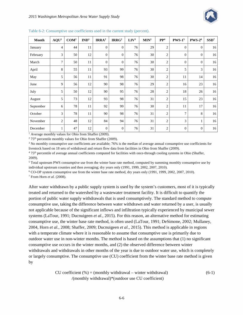
2015 Washington Metropolitan Area Water Supply Study
Table 6-2: Consumptive use coefficients used in the current study (percent).
Month AQU1 COM2 IND1 IRRA2 IRRG2 LIV3 MIN1 PP4 PWS-15 PWS-26 SSD7
January 4 44 11 0 0 76 29 2 0 0 16
February 3 50 12 0 0 76 30 2 0 0 16
March 7 50 11 0 0 76 30 2 0 0 16
April 8 55 11 93 99 76 30 2 5 3 16
May 5 56 11 91 98 76 30 2 11 14 16
June 9 56 12 90 98 76 29 2 16 23 16
July 5 50 12 90 95 76 28 2 18 26 16
August 5 73 12 93 98 76 31 2 15 23 16
September 6 78 11 92 99 76 30 2 11 17 16
October 3 78 11 90 98 76 31 2 7 8 16
November 2 48 12 84 94 76 31 2 3 1 16
December 1 47 12 0 0 76 31 2 0 0 16 1 Average monthly values for Ohio from Shaffer (2009). 2 75th percentile monthly values for Ohio from Shaffer (2009). 3 No monthly consumptive use coefficients are available; 76% is the median of average annual consumptive use coefficients for livestock based on 18 sets of withdrawal and return flow data from facilities in Ohio from Shaffer (2009). 4 75th percentile of average annual coefficients computed for facilities with once-through cooling systems in Ohio (Shaffer, 2009). 5 Total upstream PWS consumptive use from the winter base rate method, computed by summing monthly consumptive use by individual upstream counties and then averaging; dry years only (1991, 1999, 2002, 2007, 2010). 6 CO-OP system consumptive use from the winter base rate method, dry years only (1991, 1999, 2002, 2007, 2010). 7 From Horn et al. (2008).
After water withdrawn by a public supply system is used by the system’s customers, most of it is typically treated and returned to the watershed by a wastewater treatment facility. It is difficult to quantify the portion of public water supply withdrawals that is used consumptively. The standard method to compute consumptive use, taking the difference between water withdrawn and water returned by a user, is usually not applicable because of the significant inflows and infiltration typically experienced by municipal sewer systems (LaTour, 1991; Ducnuigeen et al., 2015). For this reason, an alternative method for estimating consumptive use, the winter base rate method, is often used (LaTour, 1991; DeSimone, 2002; Mullaney, 2004, Horn et al., 2008; Shaffer, 2009; Ducnuigeen et al., 2015). This method is applicable in regions with a temperate climate where it is reasonable to assume that consumptive use is primarily due to outdoor water use in non-winter months. The method is based on the assumptions that (1) no significant consumptive use occurs in the winter months, and (2) the observed difference between winter withdrawals and withdrawals in other months of the year is due to outdoor water use, which is completely or largely consumptive. The consumptive use (CU) coefficient from the winter base rate method is given by
CU coefficient (%) = (monthly withdrawal – winter withdrawal) (6-1) /(monthly withdrawal)*(outdoor use CU coefficient)
6-6

2015 Washington Metropolitan Area Water Supply Study
This study defines the winter withdrawal rate as the average of December through February withdrawals, and assumes that outdoor use is 100 percent consumptive. The winter base rate method has some obvious limitations. For example, it does not take into account consumptive use that does not vary seasonally, as might occur for a public supply system that supplies a large industrial facility whose consumptive use is constant.
Monthly consumptive use coefficients for Potomac basin public water suppliers were calculated in this study using the winter base rate method. Selected results appear in Table 6-3, which also includes results from Shaffer’s study. The coefficients for total PWS withdrawals upstream of WMA intakes, for both an average year and a dry year, are given in columns four and five of Table 6-3. The methodology used to compute these coefficients is described in Appendix D. The dry year coefficients in column five also appear in Table 6-2 in column 10 under “PWS-1,” and were used to compute the estimates of current annual and summer upstream consumptive use for the PWS sector given in Table 6-1. The coefficients for the CO-OP suppliers appear in columns six and seven of Table 6-3. The CO-OP suppliers’ dry year coefficients also appear in Table 6-2 in column 11 under “PWS-2,” and were used in the forecast of consumptive use in the PWS sector, as discussed in the next section. The last three columns of Table 6-3 give consumptive use coefficients calculated for three individual upstream suppliers – Loudoun Water, Rockville, and Leesburg – that are supplied by intakes in the Potomac River and for which there is fairly high quality data available.4
Figure 6-2: Estimated total PWS withdrawals upstream of WMA intakes.
Results in Table 6-3 provide a comparison of PWS consumptive use coefficients for various systems. Mean consumptive use coefficients for the CO-OP system are reasonably close to median values obtained by Shaffer (2009) and dry year coefficients are close to Shaffer’s 75th percentile values. Consumptive use coefficients computed for total upstream PWS withdrawals are lower than the USGS coefficients and
4 For the years in which data were available, Loudoun Water actually purchased most of its water from Fairfax Water. However, separate consumptive use coefficients for Loudoun Water’s total demand could be calculated from data it provided for this study. Leesburg withdrawals are also included in the calculation of upstream consumptive use by county.
0
20
40
60
80
100
120
140
1990 1995 2000 2005
PWS
With
draw
als,
MG
D
6-7
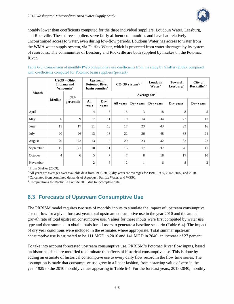
2015 Washington Metropolitan Area Water Supply Study
notably lower than coefficients computed for the three individual suppliers, Loudoun Water, Leesburg, and Rockville. These three suppliers serve fairly affluent communities and have had relatively unconstrained access to water, even during low-flow periods. Loudoun Water has access to water from the WMA water supply system, via Fairfax Water, which is protected from water shortages by its system of reservoirs. The communities of Leesburg and Rockville are both supplied by intakes on the Potomac River.
Table 6-3: Comparison of monthly PWS consumptive use coefficients from the study by Shaffer (2009), compared with coefficients computed for Potomac basin suppliers (percent).
Month
USGS – Ohio, Indiana and Wisconsin1
Upstream Potomac River basin counties2
CO-OP system2, 3 Loudoun Water2
Town of Leesburg2
City of Rockville2, 4
Median 75th percentile
Average for
All years
Dry years All years Dry years Dry years Dry years Dry years
April 4 5 3 3 18 8 5
May 6 9 7 11 10 14 34 22 17
June 15 17 11 16 17 23 43 33 16
July 20 26 13 18 22 26 48 38 21
August 20 22 13 15 20 23 42 33 22
September 15 21 10 11 15 17 37 26 17
October 4 6 5 7 7 8 18 17 10
November 2 3 2 1 6 8 2 1 From Shaffer (2009). 2 All years are averages over available data from 1990-2012; dry years are averages for 1991, 1999, 2002, 2007, and 2010. 3 Calculated from combined demands of Aqueduct, Fairfax Water, and WSSC. 4 Computations for Rockville exclude 2010 due to incomplete data.
Forecasts of Upstream Consumptive Use
The PRRISM model requires two sets of monthly inputs to simulate the impact of upstream consumptive use on flow for a given forecast year: total upstream consumptive use in the year 2010 and the annual growth rate of total upstream consumptive use. Values for these inputs were first computed by water use type and then summed to obtain totals for all users to generate a baseline scenario (Table 6-4). The impact of dry year conditions were included in the estimates where appropriate. Total summer upstream consumptive use is estimated to be 111 MGD in 2010 and 141 MGD in 2040, an increase of 27 percent.
To take into account forecasted upstream consumptive use, PRRISM’s Potomac River flow inputs, based on historical data, are modified to eliminate the effects of historical consumptive use. This is done by adding an estimate of historical consumptive use to every daily flow record in the flow time series. The assumption is made that consumptive use grew in a linear fashion, from a starting value of zero in the year 1929 to the 2010 monthly values appearing in Table 6-4. For the forecast years, 2015-2040, monthly
6-8
2015 Washington Metropolitan Area Water Supply Study
consumptive use is estimated from the 2010 value and the growth rate, and is then subtracted from the flow time series. The 2010 monthly values and the annual growth rates are given in the fifth and sixth columns of Table 6-4.
The forecasts of consumptive use by water use type required assumptions concerning future growth in each use sector, as discussed in more detail in Appendix D. It was assumed that no growth would occur for the following three use types: AQU, IND, IRRA, consistent with a review of available withdrawal time series data and other considerations. No growth for the IRRA sector is a preliminary assumption that may be revised when a new forecast becomes available later this year (see below). It was assumed that growth in the following sectors would occur at the same rate as projected population growth in the upstream portion of the basin: COM, IRRG, LIV, MIN, and SSD. The projected population growth rate in the upper Potomac River basin over the period 2010-2040, excluding areas served by the CO-OP suppliers, was estimated to be 35 percent. In the cases of agricultural irrigation and water use for livestock, new estimates of growth will be available later in 2015 from an analysis by the U.S. Department of Agriculture being conducted for the Chesapeake Bay Program. It is planned that these growth rates will be incorporated into final consumptive use values presented in ICPRB’s basin-wide comprehensive plan.
More detailed assumptions were used in the projections for PWS, as discussed in Appendix D. Separate forecasts were made for the counties bordering the Potomac River or its North Branch and for those that do not border these streams. The counties that border the Potomac River and the North Branch have access to an ample supply of water during droughts relative to their potential needs due to the Potomac River’s large drainage area and the regulation of low flows by Jennings Randolph and Savage reservoirs. Therefore, it was assumed that in the future in a dry year, their consumptive use coefficients would be similar to those of the CO-OP suppliers (column 11 in Table 6-2 and column seven in Table 6-3). It was assumed that the dry year consumptive use patterns of counties not bordering the Potomac River would not change from their estimated present values (column 10 in Table 6-2 and column five in Table 6-3).
Chapter 3 presents a forecast of declining household indoor water use rates and discusses how this decline is incorporated into forecasts of WMA demand in future years. Because the estimates for upstream PWS consumptive demand presented in the current chapter are based on assumed seasonal changes in outdoor use, declines in indoor use are not incorporated into the forecast for upstream consumptive use in the PWS sector.
There is considerable uncertainty in any estimate of current or future consumptive use. Therefore, the assessment of the ability of the WMA system to meet future needs, presented in Chapter 1, includes a sensitivity test of the impact of future upstream consumptive use. This sensitivity test considers two alternative consumptive use growth scenarios: a high growth scenario and a low growth scenario. Monthly annual growth rates and monthly values for total upstream consumptive use under these scenarios are given in Table 6-4. Forecasted 2040 upstream consumptive use in the low and high scenarios are –10 percent and +15 percent of the baseline scenario, respectively. Growth rates may be higher than the baseline forecast, for example, if several municipalities in the upper Potomac River basin implement water reuse plans to raise revenue and help meet their nutrient discharge limits, with the various purchasers using the treated wastewater for irrigation, power generation, and other highly consumptive purposes. Growth rates of upstream consumptive use may be lower than the baseline
6-9

2015 Washington Metropolitan Area Water Supply Study
forecast, for example, if several upstream municipalities construct water storage facilities to reduce their systems’ vulnerability to drought, and/or if adoption of residential solar power systems becomes widespread, reducing demand for power generated by thermoelectric facilities located in the Potomac River basin.
Table 6-4: Estimates of monthly upstream consumptive use (MGD) in 2010 and growth rates (MGD/yr).
Month
Previous study (Steiner et al., 2000)
Baseline scenario for upstream CU
Low upstream CU growth scenario
High upstream CU growth scenario
2010 Annual growth 2040 2010 Annual
growth 2040 Annual growth 2040 Annual
growth 2040
January 44 0.2 50 53 0.45 66 0.07 55 0.58 70
February 44 0.2 50 54 0.46 67 0.04 55 0.55 70
March 44 0.2 50 53 0.45 66 0.05 55 0.55 69
April 44 0.2 50 63 0.50 78 0.03 64 0.62 82
May 44 0.2 50 76 0.73 98 0.26 84 1.04 107
June 139 1.0 169 104 0.98 133 0.46 118 1.55 151
July 139 1.0 169 114 1.02 145 0.45 128 1.64 163
August 139 1.0 169 115 1.03 146 0.40 127 1.57 162
September 44 0.2 50 94 0.86 120 0.28 103 1.23 131
October 44 0.2 50 73 0.61 91 0.16 77 0.87 99
November 44 0.2 50 63 0.48 76 0.04 64 0.63 82
December 44 0.2 50 56 0.46 70 0.07 58 0.60 74
Average 68 0.4 80 76 0.7 96 0.2 82 1.0 105
Summer average 139 1.0 169 111 1.0 141 0.4 124 1.6 159
6-10
2015 Washington Metropolitan Area Water Supply Study
7 Climate Change
Evidence indicates that the Earth has been warming over the past century. This warming is causing the melting of mountain glaciers and sea ice in many parts of the world, a rise in sea levels, and changes in patterns of precipitation. Most scientists agree that these trends are likely to continue and to accelerate largely due to increasing levels of carbon dioxide and other “greenhouse” gases in our atmosphere. Of the potential consequences of climate change, water resources related impacts (availability, use, and management) are among the most significant. The current study includes an analysis of the potential alterations of Potomac basin stream flows due to climate change and the resulting impact on the ability of the WMA water supply system to meet future demands.
CO-OP conducted an assessment of the potential impact of climate change on regional water supplies in Part 2 of the 2010 study (Ahmed et al., 2013). This assessment used output from six different general circulation models (GCMs) which had been downscaled to the Chesapeake Bay region by the USGS’s National Research Program. The downscaled GCM output provided 18 separate projections of future temperature and precipitation changes in the Potomac River basin. GCMs have been constructed by teams of scientists throughout the world to simulate the physical processes which affect the global climate. They also incorporate projections of future economic, technological, and societal changes to construct scenarios of future global greenhouse gas emissions. In this previous assessment, CO-OP relied on the Chesapeake Bay Program Watershed Model (Phase 5.2) to simulate the effects of changing precipitation and temperature on Potomac River basin stream flows. PRRISM was used to assess the impact of the resulting altered stream flow scenarios on the current WMA water supply system.
Part 2 of the 2010 demand study was limited in its ability to provide water resource managers with information that they could use to inform planning decisions. Although 18 is considered a relatively large number of climate projections (Gleckler et al., 2008), the results were difficult to incorporate from a planning perspective because there were a wide range of projected impacts, with scenario results evenly divided between no impact, moderate impact, and major impact. Also, the projections from the GCMs had been scaled down to the watershed level using historical daily variability in weather from the period 1988-1999. This relatively short time period includes a moderate drought, occurring in 1999, but does not capture the full range of conditions that could be experienced in 2040 under an altered climate.
One goal of the sensitivity analysis described in this chapter and in Section 8.4 is to assess the ability of the current water supply system to meet forecasted demands under climate change in the event of a severe and prolonged drought. Basin-wide percent changes in stream flow are applied to the natural historic stream flow records used in PRRISM and the sensitivity of system performance metrics is determined. Changes in long-term average stream flow are linked to potential changes in temperature and precipitation by means of climate response functions, developed from Watershed Model output for the previous study’s 18 climate change projections. Thus, the sensitivity test results identify the range of climate conditions that may have a large enough impact to warrant preventative actions. They also provide the region’s WMA water resource managers with information that can help them interpret new climate projections and research results on long-term hydrological trends as they become available.
7-1

2015 Washington Metropolitan Area Water Supply Study
Approach
The assessment of potential climate change impacts was accomplished by conducting a sensitivity test informed by hydrologic modeling results from Part 2 of the 2010 study. The assessment was conducted in four steps:
1. Watershed Model stream flow predictions were averaged over the model simulation period 1988-1999 to derive percent changes for the 18 climate projections from Part 2 of the 2010 study.
2. As a verification step, PRRISM was used to show that values of key system performance metrics obtained using simple seasonal stream flow change factors are comparable to those obtained using Watershed Model stream flow output from Part 2 of the 2010 study.
3. A climate response function was developed to relate percent change in seasonal stream flow to changes in precipitation and temperature.
4. The vulnerability of the WMA system to climate change was determined by applying a range of percent changes in seasonal stream flow to the full 1929-2013 historic stream flow time series used in PRRISM.
The analysis included a verification step which demonstrated that simple basin-wide seasonal changes in stream flow, as opposed to the spatially-varying daily changes from the Watershed Model, could predict system storage reductions similar to those seen in Part 2 of the 2010 study. As discussed below, analyses indicated that the use in PRRISM of seasonal percent changes provided a better match to Part 2 results than use of annual stream flow changes. Once it was demonstrated that results were not significantly different, a regression equation relating precipitation and temperature change to seasonal stream flow change was developed. This representation of the system and its response to changing climate conditions has been termed a climate response function (Brown et al., 2011). In order to assess system vulnerability to climate change, PRRISM-input stream flow values were incrementally varied, on a basin-wide, seasonal basis, over a plausible range, determined by the climate change projections and climate response function. The climate conditions under which certain stream flow reductions caused system failure (e.g., minimum storage of zero or Potomac River shortfalls) were noted. Using these results the climate space, or realm of future possible climate conditions, can be associated with risk (in the case of performance metrics not being met). Thus, the climate response function allows an assessment of system vulnerabilities over a wide range of possible climate futures, not just the small number that was available in the GCM analysis of Part 2 of the 2010 demand study.
Potential Changes in Stream Flow
The current analysis uses as its starting point the Watershed Model stream flow predictions from Part 2 of the 2010 study. Watershed Model output included simulations of daily stream flow for each of the study’s 18 climate scenarios over the 12-year simulation period, 1988-1999, at many points along the Potomac River and along many of the river’s tributaries. The first four columns of Table 7-1, below, show the average annual changes in temperature and precipitation for each of the 18 climate scenarios, along with changes in basin-wide average annual stream flow predicted by the Watershed Model as presented in Part 2 of the demand 2010 study. Table 7-1 also contains three new flow results which were calculated from Watershed Model output: percent changes in average annual flow at Little Falls and average changes at Little Falls for two seasonal periods. The seasonal periods were defined as summer (June, July,
7-2

2015 Washington Metropolitan Area Water Supply Study
August) and an “other month” period. These stream flow percent changes were calculated based on natural Little Falls flow. Natural Little Falls flow is defined as observed flow at the USGS stream gage (Site ID 01646500) at Little Falls dam with adjustments made to remove the effects of WMA withdrawals and North Branch reservoir releases. Little Falls dam is also the location of the most downstream WMA water supply intake.
It should be noted that much of the reduction in stream flow reported in Table 7-1 is due to the simulated increase in evapotranspiration caused by rising temperatures. Results from some recent modeling studies indicate that the simple model of evapotranspiration used in the current version of the Watershed Model may be over-estimating this effect (de Boer et al., 2011; Wu et al., 2013; Butcher et al., 2014). Evapotranspiration is the combined loss of water to the atmosphere from evaporation from land and water surfaces and from transpiration, that is, the release of water to the atmosphere by vegetation. However, the response of transpiration to climate change is complex (Reich et al., 2006; Ainsworth and Rogers, 2007; de Boer et al., 2011). Increasing levels of carbon dioxide (CO2) will increase plant photosynthesis but decrease the density and apertures of leaf stomata, reducing diffusion of water vapor from leaves. The impact of the combined effects of increasing temperatures and increasing levels of CO2 on watershed hydrology is an active area of research. The Chesapeake Bay Program Watershed Model does not currently take into account the effects of rising CO2.
All values reported in Table 7-1, with the exception of temperature, are given as percent change from baseline scenario results. One difference between this study and the last study is the baseline scenario used to represent the “without” climate change condition for comparison with the 18 “with” climate change conditions. The baseline scenario for this study applies the monthly change factors derived from the 1988-1999 historical period from the Watershed Model to the full 1929-2013 historical period present in PRRISM rather than the simulated baseline conditions, based on the 1988-1999 historical period from the Watershed Model, used in the previous study.
Table 7-1 allows a comparison of changes in basin-wide average annual stream flow and changes in natural annual average Potomac River flow at Little Falls dam, given in columns four and five. These two sets of values are reasonably close. The average annual values were not used for the current analysis because the effects on stream flow during the summer months were too muted by the other months. The changes in seasonal Little Falls flow averages, given in the last two columns of Table 7-1, are shown in the next section to be useful surrogate measures of seasonal basin-wide flow averages.
7-3
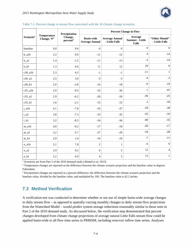
2015 Washington Metropolitan Area Water Supply Study
Table 7-1: Percent change in stream flow associated with the 18 climate change scenarios.
Scenario1 Temperature Change, oF2
Precipitation Change, percent3
Percent Change in Flow
Basin-wide Average Annual
Average Annual - Little Falls
Average Summer - Little
Falls
“Other Month” - Little Falls
baseline 0.0 0.0 0 0 0 0
b_a1b 2.2 0.0 -11 -12 4 -14
b_a2 1.4 -1.2 -11 -13 -3 -14
b_b1 1.3 6.6 11 12 29 9
c30_a1b 2.3 4.3 -1 -1 -11 1
c30_a2 2.5 3.6 -3 -3 -4 -3
c30_b1 2.0 -2.8 -16 -18 -9 -19
c35_a1b 2.9 -9.5 -35 -36 1 -41
c35_a2 2.9 -6.2 -26 -26 -36 -25
c35_b1 1.6 -2.1 -15 -15 2 -18
i_a1b 4.1 -7.8 -35 -37 -29 -38
i_a2 3.8 -7.3 -33 -35 -43 -34
i_b1 3.2 -8.5 -34 -36 -40 -35
m_a1b 4.0 -0.2 -17 -18 -28 -17
m_a2 3.2 -5.7 -27 -29 -34 -28
m_b1 2.9 1.4 -10 -10 -7 -11
n_a1b 3.1 7.8 2 1 6 0
n_a2 2.9 9.2 6 5 12 4
n_b1 2.2 6.9 4 3 13 1
1 Scenarios are from Part 2 of the 2010 demand study (Ahmed et al. 2013) 2 Temperature changes are reported as the difference between the climate scenario projection and the baseline value in degrees Fahrenheit. 3 Precipitation changes are reported as a percent difference: the difference between the climate scenario projection and the baseline value, divided by the baseline value, and multiplied by 100. The baseline value is 42.2 inches.
Method Verification
A verification test was conducted to determine whether or not use of simple basin-wide average changes to daily stream flow – as opposed to spatially-varying monthly changes to daily stream flow projections from the Watershed Model – would predict system storage reductions reasonably similar to those seen in Part 2 of the 2010 demand study. As discussed below, the verification step demonstrated that percent changes developed from climate change projections of average natural Little Falls stream flow could be applied basin-wide to all flow time series in PRRISM, including reservoir inflow time series. Analyses
7-4

2015 Washington Metropolitan Area Water Supply Study
indicated that the use of seasonal stream flow change factors provided a better match to Part 2 results than use of change factors for average annual flow.
The summer and “other month” change factors, derived from the percent changes in the last two columns of Table 7-1, were used in PRRISM. The resulting predictions of system reservoir storages were comparable to those found in Part 2 of the 2010 demand study. Figure 7-1 compares minimum combined Jennings Randolph water supply storage and Little Seneca Reservoir storage for two different PRRISM runs. The first run results were taken directly from Tables 6-5 through Table 6-7 in Part 2 of the 2010 demand study. The second run used baseline input time series with the seasonal stream flow change factors applied. For the runs with Potomac deficits, an additional storage amount, equal to the Potomac deficit, was subtracted from the storage total. This resulted in a negative value which provided an indication of the system’s storage deficit.
Figure 7-1: Projections of minimum combined Jennings Randolph water supply storage and Little Seneca Reservoir storage, given 2040 demands.
The two projections of minimum water supply storage in Figure 7-1 are similar, though minimum storages from the verification run tend to be higher than those predicted in Part 2 of the 2010 study. To compare the two sets of data, linear regression analyses were conducted. The basic statistics appear in
-4
-2
0
2
4
6
8
10
12
14
4 5 6 7 8 9 10 11
Jenn
ings
Ran
dolp
h w
ater
sup
ply
and
Littl
e Se
neca
Res
ervo
ir m
in. s
tora
ge, B
G
Little Falls annual average flow, BGD
Part 2 of the 2010 Study Verification for 2015 Study
Linear (Part 2 of the 2010 Study) Linear (Verification for 2015 Study)
7-5

2015 Washington Metropolitan Area Water Supply Study
Table 7-2, where SE stands for standard error, R2 stands for the coefficient of determination, and n is the sample size for each model. Although not shown in Table 7-2, all p-values were below 0.05, which indicates that the intercepts and slopes of the linear regressions are significant at the 95 percent confidence level.
Table 7-2: Statistics for the linear regression analyses on the two minimum storage projections.
Model Intercept, α Slope, β SEintercept SEslope R2 n
Part 2 of the 2010 Study -14.44 2.32 1.63 0.21 0.88 19
Verification for the 2015 Study -12.17 2.38 3.28 0.42 0.65 19
Next two tests were formulated to see if the parameters from the two models differ significantly. The first test is applied to the slope and the second test is applied to the intercept. The structure of the null and alternative hypotheses are the same: the null hypothesis (Ho) is that the parameter for the Part 2 model (β1 or α1) is the same as the parameter for the verification model for the 2015 study (β2 or α2 ); the two-sided alternative hypothesis (Ha) is that the parameters are not equal. The test statistic for both hypotheses is the student’s t, which required a calculation of pooled variances for the two datasets and used a sample size N equal to the sum of the two sample set sizes n.
The test statistics and outcome for both parameters are summarized in Table 7-3. The null hypothesis for both the slopes and intercepts were accepted at the two-tailed five percent confidence level, indicating that neither parameter was significantly different between the two models.
Table 7-3: Two-sided hypothesis tests comparing the slopes and intercepts from Part 2 of the 2010 demand study and from the verification test.
Parameter Null hypothesis
Two-sided alternative hypothesis
Standard error of difference Student’s t N Critical t
(5%) Outcome
Slope, β Ho: β1=β2 Ha: β1<>β2 0.47 -0.13 34 ±2.03 Accept Ho
Intercept, α Ho: α1=α2 Ha: α1<>α2 3.66 -0.62 34 ±2.03 Accept Ho
Projected Changes in Temperature & Precipitation
The precipitation and temperature changes shown in Table 7-1 were obtained by computing area-weighted averages of changes for Potomac River basin land segments from the Watershed Model, as described in Part 2 of the 2010 study. The calculations were restricted to areas upstream of the USGS stream gage (Station ID 01646500) on the Potomac River at Little Falls dam near Washington, D.C. The temperature and precipitation climate change projections used in the Watershed Model were developed by the USGS’s National Research Program for the Chesapeake Bay Program.
Figure 7-2 is a plot of changes in temperature and precipitation for scenarios used in Part 2 of the 2010 demand study. For comparison, projected temperature and precipitation changes from another study are also shown. This second study (WRF, 2013) was conducted for the Water Research Foundation (WRF) and led by the firm, Hydrologics, Inc., in partnership with Riverside Technologies, Inc. and Hazen and
7-6
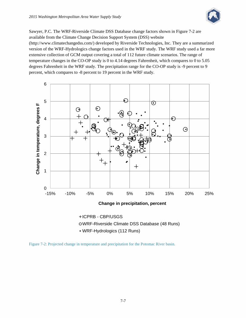
2015 Washington Metropolitan Area Water Supply Study
Sawyer, P.C. The WRF-Riverside Climate DSS Database change factors shown in Figure 7-2 are available from the Climate Change Decision Support System (DSS) website (http://www.climatechangedss.com/) developed by Riverside Technologies, Inc. They are a summarized version of the WRF-Hydrologics change factors used in the WRF study. The WRF study used a far more extensive collection of GCM output covering a total of 112 future climate scenarios. The range of temperature changes in the CO-OP study is 0 to 4.14 degrees Fahrenheit, which compares to 0 to 5.05 degrees Fahrenheit in the WRF study. The precipitation range for the CO-OP study is -9 percent to 9 percent, which compares to -8 percent to 19 percent in the WRF study.
Figure 7-2: Projected change in temperature and precipitation for the Potomac River basin.
0
1
2
3
4
5
6
-15% -10% -5% 0% 5% 10% 15% 20% 25%
Cha
nge
in te
mpe
ratu
re, d
egre
es F
Change in precipitation, percent
ICPRB - CBP/USGSWRF-Riverside Climate DSS Database (48 Runs)WRF-Hydrologics (112 Runs)
7-7

2015 Washington Metropolitan Area Water Supply Study
Climate Response Function
Climate response functions were developed for average summer season (June, July, August) and “other month” Potomac basin stream flow. The response function for summer flow was obtained by applying a least squares regression analysis to the data in columns two, three, and six of Table 7-1. The resulting equation for percent change in the average summer flow at Little Falls dam, Qsummer, is:
∆Qsummer = 2.254 * ∆P – 0.038 * ∆T (7-2)
where ∆P is the percent change in precipitation and ∆T is the change in temperature in degrees Fahrenheit. The p-values for these slope coefficients are 0.0003 and 0.0025, respectively. The zero intercept equation was determined to be appropriate from a conceptual point of view since the assumed response in the baseline case is zero. The alternative equation had an intercept with a p-value greater than 0.05, which indicates that the intercept is not significantly different from zero.
A response function for flow in other months was obtained from a regression analysis relating average summer flow at Little Falls dam to flow in the remaining months, using the data in columns six and seven of Table 7-1. The equation is
∆Qother = 0.752 * ∆Qsummer (7-3)
where ∆Qother is the percent change in average flow at Little Falls dam for the months of September through May. The p-value for the slope is 7.0e-5, where the assumption was again made that the intercept of the equation was zero.
Figure 7-3 shows a plot of the “other month” flow changes to the summer month flow changes for the 18 climate projections from Part 2 of the 2010 demand study (given in the last two columns of Table 7-1). This figure also shows the regression line for Equation (7-3).
7-8

2015 Washington Metropolitan Area Water Supply Study
Figure 7-3: Other month flow percent change versus summer percent change.
Values computed from the climate response functions, equations (7-2) and (7-3), are given in Table 7-4 and Table 7-5. The ranges of changes in temperature and precipitation used in these tables are consistent with the ranges of projected changes in the 18 scenarios used in Part 2 of the 2010 study. The computed ranges for percent change in Potomac River basin stream flow is -38 percent to +23 percent for the summer season (Table 7-4) and -28 percent to +17 percent for the “other month” period (Table 7-5). These ranges are used in the climate change sensitivity analysis presented in Section 8.4.
Table 7-4: Percent changes in average summer flow at Little Falls dam.
Precipitation Change, Percent
-10.0 -7.5 -5.0 -2.5 0.0 2.5 5.0 7.5 10.0
Tem
pera
ture
Cha
nge,
°F
0.0 -23 -17 -11 -6 0 6 11 17 23
0.5 -24 -19 -13 -8 -2 4 9 15 21
1.0 -26 -21 -15 -9 -4 2 7 13 19
1.5 -28 -23 -17 -11 -6 0 6 11 17
2.0 -30 -24 -19 -13 -8 -2 4 9 15
2.5 -32 -26 -21 -15 -9 -4 2 7 13
3.0 -34 -28 -23 -17 -11 -6 0 6 11
3.5 -36 -30 -24 -19 -13 -8 -2 4 9
4.0 -38 -32 -26 -21 -15 -9 -4 2 7
y = 0.7519xR² = 0.5942
-50%
-40%
-30%
-20%
-10%
0%
10%
20%
30%
-50% -40% -30% -20% -10% 0% 10% 20% 30% 40%
Oth
er m
onth
pe
rcen
t cha
nge
in fl
ow
Summer month percent change in flow
7-9
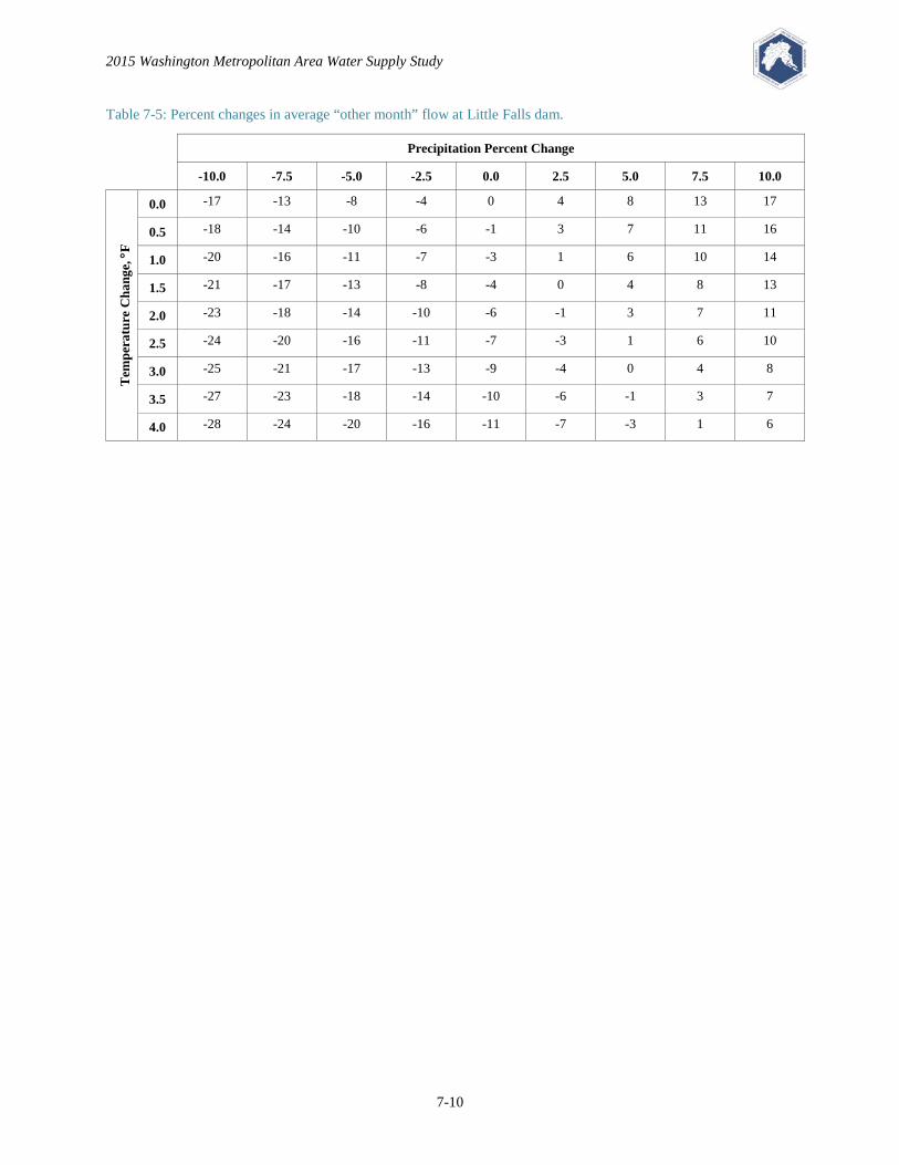
2015 Washington Metropolitan Area Water Supply Study
Table 7-5: Percent changes in average “other month” flow at Little Falls dam.
Precipitation Percent Change
-10.0 -7.5 -5.0 -2.5 0.0 2.5 5.0 7.5 10.0
Tem
pera
ture
Cha
nge,
°F
0.0 -17 -13 -8 -4 0 4 8 13 17
0.5 -18 -14 -10 -6 -1 3 7 11 16
1.0 -20 -16 -11 -7 -3 1 6 10 14
1.5 -21 -17 -13 -8 -4 0 4 8 13
2.0 -23 -18 -14 -10 -6 -1 3 7 11
2.5 -24 -20 -16 -11 -7 -3 1 6 10
3.0 -25 -21 -17 -13 -9 -4 0 4 8
3.5 -27 -23 -18 -14 -10 -6 -1 3 7
4.0 -28 -24 -20 -16 -11 -7 -3 1 6
7-10
2015 Washington Metropolitan Area Water Supply Study
8 Results
The resource analysis presented in this chapter uses PRRISM simulations to evaluate how the WMA’s current system of water supply resources would respond to forecasted water demands under the range of hydrologic conditions that occurred from 1929 through 2013. It also assesses the vulnerability of the system to changes in stream flow that might occur during a severe, prolonged drought in a basin altered by global climate change. Forecasts of average annual WMA demands, computed using MWCOG Round 8.3 demographic projections, were presented in Chapter 3. These annual forecasts, combined with estimates of seasonal and daily variations in demand described in Chapter 4, are used in PRRISM to generate a time series of daily withdrawals for a specified forecast year. PRRISM also simulates daily Potomac River flows, reservoir inflows, and system operations under the assumptions discussed in Chapter 5. This includes releases made to maintain the recommended minimum flow at Little Falls dam. The system was also evaluated to examine the sensitivity of results to changes in the assumed growth rate of upstream consumptive demand, as described in Chapter 6. Unless otherwise noted, all simulations use the set of PRRISM input parameters given in Appendix F.
Model Run Overview & Measures of Performance (Metrics)
Each PRRISM run simulates daily flows, demands, and system operations over an 84-year simulation period. As discussed in Chapter 4, the simulated water supply demands include a randomly generated component of demand; therefore, each model run is based on a slightly different 84-year time series of daily WMA demands. These demand time series represent the potential variation of demand for a given set of meteorological conditions, incorporating the randomness inherent in the original demand data set. (Section 4.5 and Section 4.6 provide more detail on the random component of demand.) Since demands and corresponding results are slightly different in each PRRISM simulation, the model is run 20 times and results are presented in terms of the average and standard deviation over the 20 runs.
PRRISM simulation results are expressed in terms of metrics that provide information on the reliability, vulnerability, and resiliency of the WMA water supply system, where these terms are consistent with those used in the water resources literature (Hashimoto et al., 1982). Reliability is the statement of probability of meeting a given demand, expressed as a percentage of time the demand can be met. Vulnerability is a measure of the magnitude or significance of a failure. Resiliency gages the ability of the system to recover from system failure, and can be defined as the maximum number of consecutive periods of shortage during a simulation (Wurbs, 1996). PRRISM output metrics are described below. In these descriptions, a “Potomac deficit” is defined as the difference on any given day between the amount of water needed from the Potomac River and the amount available, where the amount needed is the sum of Potomac demands and the 100 MGD environmental flow-by at Little Falls.
WMA water supply system performance metrics: • Percentage of years with no Potomac deficits. This metric is a measure of reliability, expressed as
a percentage of years in the 84-year simulation period in which all demand is met.
8-1
2015 Washington Metropolitan Area Water Supply Study
• Maximum number of days in a row with Potomac deficits. This metric is a measure of resiliency, expressed as the maximum number of consecutive days over the simulation period in which demand cannot be met.
• Number of days in which Potomac deficits must be allocated. This metric is a measure of the vulnerability of the system, expressed as the number of consecutive and non-consecutive days a shortfall exists.
• Maximum amount of deficit allocated in a single day, MGD. This metric is a measure of the vulnerability of the system, expressed as the maximum shortfall for any single day over the simulation period.
• Total amount of deficit allocated, MG. Another measure of vulnerability, expressed as the daily amount of a shortfall summed over the course of the simulation period.
• Number of Patuxent water supply shortfalls. This metric is a measure of the vulnerability of the Patuxent Reservoir, expressed as the number of days over the simulation period with zero storage and/or the number of days where the Patuxent release is below the emergency storage request of 20 MGD.
• Number of Occoquan water supply shortfalls. This metric is a measure of the vulnerability of the Occoquan Reservoir, expressed as the number of days where the Occoquan release is below the minimum demand of 43 MGD for Occoquan’s area served.
• Number of days Patuxent plant production is less than 33 MGD. This metric is a measure of vulnerability and can be used to estimate how many days the Patuxent plant must be shut down in order to reduce its withdrawal amount.
• Percentage of years with voluntary, mandatory, and emergency restrictions. These metrics are a measure of the reliability of the system, expressed as a percentage of historical stream flow years during the simulation in which water use restrictions are implemented. For single year runs this is reported as percentage of days.
Other model run metrics include: • Jennings Randolph water supply and Little Seneca Reservoir minimum storage, BG. Minimum
combined water supply storage in the two shared reservoirs experienced over the course of the simulation period.
• Jennings Randolph water supply and Little Seneca, Occoquan, and Patuxent reservoirs minimum storage, BG. Minimum combined water supply storage in both the shared reservoirs and water supplier owned off-Potomac reservoirs experienced over the course of the simulation period.
• CO-OP maximum average annual demand, MGD. This reports the maximum of the annual averages of combined demand for Fairfax Water, Aqueduct, and WSSC that occur over the 84-year simulation period, as reduced by simulated water use restrictions. This metric does not include water produced by Fairfax Water and sold to Loudoun Water.
• Loudoun Water maximum average annual demand, MGD. This reports the maximum of the annual averages of Loudoun Water demands that occur over the 84-year simulation period, as reduced by simulated water use restrictions. This metric includes both self-serviced water as well as purchased water from Fairfax Water.
• Minimum average late summer flow with no WMA impact, MGD. This metric is the minimum, over the 84-year simulation period, of the average flow in July and August, and is the flow that
8-2
2015 Washington Metropolitan Area Water Supply Study
would have occurred without upstream reservoir releases, return flows from CO-OP supplier wastewater treatment plants, or WMA withdrawals.
• Minimum average fall flow with no WMA impact, MGD. This metric is the same flow as described above, but averaged over the months of September, October, and November.
• Minimum average late summer flow downstream of intakes, MGD. This metric is the minimum over the 84-year simulation period of the average of flow downstream of the water supply intakes in July and August and represents the simulated flow after all upstream augmentation, withdrawals, and consumptive use.
• Minimum average fall flow downstream of intakes, MGD. This metric is the same flow as described above, but averaged over the months of September, October, and November.
Model results are presented for the 20-year demand forecast, out to 2035, and also for the 25-year demand forecast, out to 2040. The 25-year forecast provides a longer planning horizon, and was possible in the current study because MWCOG Round 8.3 demographic projections were available for 2040. The 2040 year also corresponds to the forecast year used in Part 2 of the 2010 demand study. Scenarios considered in the resource assessment are described below.
Baseline 2035 & 2040 Scenarios
The ability of available water supply resources to meet forecasted demand was evaluated for two baseline scenarios. The 2035 baseline scenario assumed:
• a 20-year WMA demand forecast; • current environmental flow recommendations; • anticipated levels of conservation; • no effects of climate change on resources or demands; • implementation of voluntary, mandatory, and emergency restrictions (Section 4.7); • upstream current and future consumptive demands (Chapter 6); and • a repeat of the 1929-2013 historical stream flow record.
The 2040 baseline scenario used the same information as the 2035 baseline scenario except it was based on a 25-year forecast.
PRRISM simulation results for the two baseline scenarios are summarized in Table 8-1. Results are shown for the full simulation period of 1929-2013 historical stream flows. This table reports averages (Ave.) and the standard deviation (SD) of results from 20 model runs, where each run covers the 84-year historical period from 1929-2013.
8-3

2015 Washington Metropolitan Area Water Supply Study
Table 8-1: PRRISM results for the 2035 and 2040 baseline scenarios.1
2035 baseline 2040 baseline
Ave. (SD) Ave. (SD)
Percentage of years with no Potomac deficits, % 99.8 (0.4) 99.9 (0.3)
Max. No. of days in a row of Potomac deficits 0.0 (0.0) 0.1 (0.4)
No. of Potomac deficits 0.2 (0.4) 0.1 (0.4)
Max. amount of deficit in a single day, MGD 0.6 (1.4) 0.2 (1.0)
Total amount of deficit in full simulation period, MG 0.6 (1.4) 0.3 (1.4)
No. of Patuxent shortfalls 18.6 (0.9) 18.3 (0.7)
No. of Occoquan shortfalls 0.0 (0.0) 0.0 (0.0)
No. of days with Patuxent production < 33 MGD 3769.0 (75.8) 3861.8 (162.3)
Percentage of years with voluntary restrictions, % 4.8 (0.3) 5.3 (0.6)
Percentage of years with mandatory restrictions, % 3.2 (0.6) 3.9 (0.5)
Percentage of years with emergency restrictions, % 0.0 (0.0) 0.5 (1.0)
Little Seneca Reservoir min. storage, BG 0.9 (0.3) 0.6 (0.5)
Jennings Randolph water supply min. storage, BG 2.3 (0.2) 1.2 (0.2)
Jennings Randolph water quality min. storage, BG 2.8 (0.0) 2.8 (0.0)
Patuxent Reservoir min. storage, BG 0.0 (0.0) 0.0 (0.0)
Occoquan Reservoir min. storage, BG 2.2 (0.2) 2.0 (0.3)
Savage Reservoir min. storage, BG 0.6 (0.0) 0.6 (0.0)
Loudoun Water Quarry A min. storage, BG 0.1 (0.0) 0.1 (0.0)
Jennings Randolph water supply and Little Seneca Reservoir min. storage, BG
3.2 (0.5) 1.9 (0.6)
Jennings Randolph water supply and Little Seneca, Occoquan, and Patuxent Reservoirs min. storage, BG
7.6 (0.9) 5.8 (0.9)
CO-OP max. average annual demands, MGD 524.2 (3.2) 541.0 (4.1)
Loudoun Water max. average annual demands, MGD 32.4 (0.2) 33.0 (0.2)
Min. average late summer flow at Little Falls with no WMA impact, MGD
605.7 (0.0) 600.6 (0.0)
Min. average fall flow at Little Falls with no WMA impact, MGD
523.6 (0.0) 520.4 (0.0)
Min. average late summer flow at Little Falls, MGD 327.2 (10.5) 323.8 (13.6)
Min. average fall flow at Little Falls, MGD 257.9 (4.9) 256.1 (4.7) 1 This table reports averages (standard deviations) of results from 20 model runs, where each run covers the 84-year historical period from 1929-2013.
8-4
2015 Washington Metropolitan Area Water Supply Study
8.2.1 Minimum Reservoir Storage Levels
Minimum reservoir storage values are key system performance metrics. The minimum storage value for a given reservoir is the lowest storage volume predicted to occur during an 84-year simulation period. Table 8-1 shows these values for each system reservoir as the average of 20 runs. Table 8-1 shows that during a repeat of the historical stream flow record, the minimum combined water supply storage in Jennings Randolph and Little Seneca Reservoir under the baseline scenario is predicted to be 3.2 BG, given 2035 demands and 1.9 BG, given 2040 demands. Table 8-1 also shows that minimum combined storage in Jennings Randolph’s water supply account, Little Seneca, Patuxent, and Occoquan reservoirs is 7.6 BG, given 2035 demands, and 5.8 BG, given 2040 demands. Predicted minimum storage in Little Seneca Reservoir is 0.9 BG, given 2035 demands, and 0.6 BG, given 2040 demands. However, it should be noted that Little Seneca Reservoir storage fell to zero during the 1930 historical year for three of the 20 model runs of the baseline 2040 scenario. Storage in the Patuxent reservoirs fell to zero at the end of the 1931 historical year due to very low inflows throughout that year in both the 2035 and 2040 baseline scenarios.
8.2.2 Water Use Restrictions
Another set of metrics shown in Table 8-1 is percentage of years with water use restrictions. These results show that as WMA and upstream demands rise, the likelihood of restrictions increases. Mandatory water use restrictions are predicted to occur on average in 3.2 percent of years for the 2035 baseline scenario and 3.9 percent of years for the 2040 baseline scenario. Emergency restrictions occur on average in 0.0 percent of years for the 2035 baseline scenario and 0.5 percent of years for the 2040 baseline scenario.
8.2.3 Potomac River Shortfalls
In both the 2035 and 2040 baseline scenarios, PRRISM simulations indicate that there is a small but finite chance of Potomac River shortfall events, that is, days in which flow could not meet demands plus the 100 MGD environmental flow-by at Little Falls. As discussed in Chapter 5, Potomac deficits are more likely in CO-OP’s latest version of PRRISM since they may occur on days in which the one-day flow forecast is poor. In the version of PRRISM used for the 2010 demand study, Potomac deficits would not occur unless Little Seneca Reservoir was empty. Table 8-1 shows that for the 2035 baseline scenario, the 20 model runs predict that the Potomac River could not meet demands on an average of 0.2 days over the simulation period; in the 2040 scenario a deficit occurred on average on 0.1 days. The average total predicted shortfall in both the 2035 and 2040 baseline scenarios was fairly small, less than one MGD.
8.2.4 Patuxent Shortfalls & Partial Shutdowns
Patuxent reservoir shortfalls occur in both the 2035 and 2040 baseline scenario runs. Patuxent shortfalls occur on days in which the Patuxent reservoirs are empty or nearly empty and the Potomac River would need to supply essentially all of WSSC’s demands. Model simulations predict that the Patuxent reservoirs would have an average of 18.6 days of shortfalls over the 84-year simulation period in the 2035 baseline scenario and 18.3 days in the 2040 baseline scenario. A detailed examination of PRRISM simulation time series shows that the emptying of the Patuxent reservoirs occurs at the end of the year of the 1931 historical hydrology due to very low inflows throughout that year in both the 2035 and 2040 baseline
8-5

2015 Washington Metropolitan Area Water Supply Study
scenarios. Partial Patuxent plant shutdowns were also tracked as the number of days the Patuxent water treatment plant production was less than 33 MGD in model simulations. Table 8-1 shows that partial Patuxent plant shutdowns occur for 3,769.0 days, given 2035 demands, and 3,861.8 days, given 2040 demands. Though the minimum Patuxent production rate is somewhat lower, at 30 MGD, 33 MGD is the minimum production rate at which the Patuxent water treatment plant is able to ramp up quickly to higher production rates (Karen Wright, personal communication, February 24, 2015), an operational flexibility that is depended upon in current drought operations.
Under normal conditions, the added demand on the Potomac River due to a partial Patuxent plant shutdown or due to zero usable storage in the Patuxent reservoirs would not be a problem. Under low-flow conditions, however, the ability to make quick load shifts to the Patuxent reservoirs can help alleviate the impact of a poor one-day flow forecast and prevent the occurrence of a Potomac River shortfall, therefore making the Patuxent reservoirs an important component of the WMA system.
Sensitivity of System Performance to Upstream Consumptive Use
An analysis was conducted to determine how sensitive system performance metrics are to uncertainties in future upstream consumptive use (see Chapter 6 for upstream consumptive use forecasts). The assumptions for the consumptive use scenarios are the same as the 2035 and 2040 baseline scenarios (as described in Section 8.2) except that daily Potomac River flows were modified in PRRISM to represent the changes due to lower and higher consumptive use. The assumed growth rates are given in Table 6-4.
Table 8-2 and Table 8-3 give average model performance metrics for low and high estimates of consumptive use, given 2035 and 2040 demands, respectively. Compared with results for the baseline scenarios in Table 8-1, minimum combined Jennings Randolph and Little Seneca water supply storage values and minimum combined system storage values are higher if upstream consumptive use is lower, and are lower if upstream consumptive use is higher. Changes are also evident in other performance metrics. Notably, the minimum average late summer and fall flows at Little Falls responds to changes in estimated upstream consumptive use. Minimum average late summer flow at Little Falls without WMA impact, that is, without reservoir releases or WMA withdrawals, is 600.6 for the 2040 baseline scenario. This value rises to 618.3 MGD with the low consumptive use forecast and falls to 582.9 MGD with the high estimate.
8-6

2015 Washington Metropolitan Area Water Supply Study
Table 8-2: PRRISM results for alternative upstream consumptive use (CU) growth rates - 2035 demands.1
2035 low upstream CU growth 2035 high upstream CU
growth
Ave. (SD) Ave. (SD)
Percentage of years with no Potomac deficits, % 99.9 (0.3) 99.9 (0.4)
Max. No. of days in a row of Potomac deficits 0.0 (0.0) 0.0 (0.0)
No. of Potomac deficits 0.1 (0.2) 0.1 (0.3)
Max. amount of deficit in a single day, MGD 0.1 (0.3) 0.6 (1.8)
Total amount of deficit in full simulation period, MG 0.1 (0.3) 0.6 (1.8)
No. of Patuxent shortfalls 18.2 (0.7) 18.6 (0.9)
No. of Occoquan shortfalls 0.0 (0.0) 0.0 (0.0)
No. of days with Patuxent production < 33 MGD 3853.2 (203.7) 3798.6 (129.3)
Percentage of years with voluntary restrictions, % 4.8 (0.4) 5.3 (0.6)
Percentage of years with mandatory restrictions, % 2.6 (0.9) 3.6 (0.0)
Percentage of years with emergency restrictions, % 0.0 (0.0) 0.2 (0.6)
Little Seneca Reservoir min. storage, BG 1.0 (0.3) 0.8 (0.4)
Jennings Randolph water supply min. storage, BG 2.8 (0.2) 1.7 (0.2)
Jennings Randolph water quality min. storage, BG 2.9 (0.0) 3.0 (0.0)
Patuxent Reservoir min. storage, BG 0.0 (0.0) 0.0 (0.0)
Occoquan Reservoir min. storage, BG 2.2 (0.3) 2.1 (0.3)
Savage Reservoir min. storage, BG 0.6 (0.0) 0.6 (0.0)
Loudoun Water Quarry A min. storage, BG 0.2 (0.0) 0.0 (0.0)
Jennings Randolph water supply and Little Seneca Reservoir min. storage, BG
3.8 (0.4) 2.6 (0.5)
Jennings Randolph water supply and Little Seneca, Occoquan, and Patuxent Reservoirs min. storage, BG
8.2 (0.8) 6.8 (0.8)
COOP max. average annual demands, MGD 522.4 (2.1) 523.8 (4.0)
Loudoun Water max. average annual demands, MGD 32.3 (0.1) 32.4 (0.2)
Min. average late summer flow at Little Falls with no WMA impact, MGD
620.4 (0.0) 590.9 (0.0)
Min. average fall flow at Little Falls with no WMA impact, MGD
535.8 (0.0) 517.1 (0.0)
Min. average late summer flow at Little Falls, MGD 327.2 (9.2) 320.9 (11.3)
Min. average fall flow at Little Falls, MGD 260.0 (7.1) 258.0 (5.3) 1 This table reports averages (standard deviations) of results from 20 model runs, where each run covers the 84-year historical period from 1929-2013.
8-7
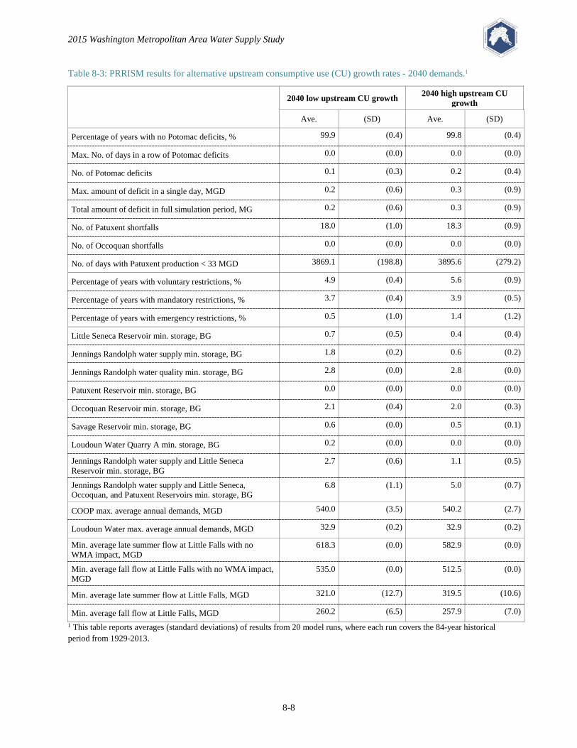
2015 Washington Metropolitan Area Water Supply Study
Table 8-3: PRRISM results for alternative upstream consumptive use (CU) growth rates - 2040 demands.1
2040 low upstream CU growth 2040 high upstream CU
growth
Ave. (SD) Ave. (SD)
Percentage of years with no Potomac deficits, % 99.9 (0.4) 99.8 (0.4)
Max. No. of days in a row of Potomac deficits 0.0 (0.0) 0.0 (0.0)
No. of Potomac deficits 0.1 (0.3) 0.2 (0.4)
Max. amount of deficit in a single day, MGD 0.2 (0.6) 0.3 (0.9)
Total amount of deficit in full simulation period, MG 0.2 (0.6) 0.3 (0.9)
No. of Patuxent shortfalls 18.0 (1.0) 18.3 (0.9)
No. of Occoquan shortfalls 0.0 (0.0) 0.0 (0.0)
No. of days with Patuxent production < 33 MGD 3869.1 (198.8) 3895.6 (279.2)
Percentage of years with voluntary restrictions, % 4.9 (0.4) 5.6 (0.9)
Percentage of years with mandatory restrictions, % 3.7 (0.4) 3.9 (0.5)
Percentage of years with emergency restrictions, % 0.5 (1.0) 1.4 (1.2)
Little Seneca Reservoir min. storage, BG 0.7 (0.5) 0.4 (0.4)
Jennings Randolph water supply min. storage, BG 1.8 (0.2) 0.6 (0.2)
Jennings Randolph water quality min. storage, BG 2.8 (0.0) 2.8 (0.0)
Patuxent Reservoir min. storage, BG 0.0 (0.0) 0.0 (0.0)
Occoquan Reservoir min. storage, BG 2.1 (0.4) 2.0 (0.3)
Savage Reservoir min. storage, BG 0.6 (0.0) 0.5 (0.1)
Loudoun Water Quarry A min. storage, BG 0.2 (0.0) 0.0 (0.0)
Jennings Randolph water supply and Little Seneca Reservoir min. storage, BG
2.7 (0.6) 1.1 (0.5)
Jennings Randolph water supply and Little Seneca, Occoquan, and Patuxent Reservoirs min. storage, BG
6.8 (1.1) 5.0 (0.7)
COOP max. average annual demands, MGD 540.0 (3.5) 540.2 (2.7)
Loudoun Water max. average annual demands, MGD 32.9 (0.2) 32.9 (0.2)
Min. average late summer flow at Little Falls with no WMA impact, MGD
618.3 (0.0) 582.9 (0.0)
Min. average fall flow at Little Falls with no WMA impact, MGD
535.0 (0.0) 512.5 (0.0)
Min. average late summer flow at Little Falls, MGD 321.0 (12.7) 319.5 (10.6)
Min. average fall flow at Little Falls, MGD 260.2 (6.5) 257.9 (7.0) 1 This table reports averages (standard deviations) of results from 20 model runs, where each run covers the 84-year historical period from 1929-2013.
8-8
2015 Washington Metropolitan Area Water Supply Study
Sensitivity of System Performance to Climate Change
The sensitivity of WMA water supply system performance to potential changes in climate was examined by conducting a series of PRRISM runs which simulated the effects of basin-wide changes in stream flow. Future changes in long-term average temperature and precipitation will lead to changes in stream flow. In Part 2 of the 2010 demand study the Chesapeake Bay Program’s Watershed Model was used to predict these changes for each of the study’s 18 climate change projections. It was shown in Chapter 7 of the current study that average changes in summer stream flow, as simulated by the Watershed Model, can be predicted with a fair degree of confidence based on changes in temperature and precipitation (equation (7-2)). For example, Table 7-4 shows that according to Watershed Model results, the percent change in average summer flow at Little Falls dam ranges from approximately -38 percent to +23 percent for the range of temperature and precipitation changes present in the 18 climate change projections used in Part 2 of the 2010 study. Corresponding changes to “other month” flow at Little Falls appear in Table 7-5.
In the current study, PRRISM inputs are altered to represent a basin-wide change in summer stream flow by applying a single percent change to all daily flow inputs, i.e. Potomac River flows and reservoir inflows, for the months of June, July, and August. This change is varied, in increments of 10 percent, from -40 percent to +30 percent to determine the response of system performance metrics. A second corresponding percent change, calculated from Equation (7-3) is applied to flow inputs for other months. In Chapter 7, results from a method verification step indicated that the use in PRRISM of simple seasonal basin-wide percent change factors produced results reasonably similar to those obtained in Part 2 of the 2010 study, which were based on the more detailed spatially and temporarily varying stream flow output from the Watershed Model. This verification step was limited to the 12-year simulation period available in the 2010 study, which only included a moderate drought. The analysis that follows assumes that the methodology can be extended to the current study’s entire 84-year simulation period.
8.4.1 PRRISM Climate Change Results
The assumptions for the climate change sensitivity test scenarios are the same as those used in the 2040 baseline scenario (see Section 8.2) except for the adjustments to stream flow. Demands were not adjusted in the current study because in Part 2 of the 2010 demand study it was shown that results were fairly insensitive to alterations in demands based on changes in climate. The overall climate change scenario development is described in more detail in Chapter 7.
The impact of the climate change sensitivity tests on WMA water supply system performance metrics are given in Table 8-4 through Table 8-8 and in Figure 8-1. Stream flow alterations represent changes in long-term average flows. The range of stream flow alterations simulated in this sensitivity test is large, from –40 to +30 percent, and according to model results, the corresponding impact on the performance of the current WMA system varies dramatically:
• If long-term average summer flows were to fall by 10 percent or more by the year 2040, simulation results indicate that during a severe drought emergency, emergency water use restrictions would occur, most system reservoirs would be drained, and on some days the system would be unable to meet demands and the 100 MGD environmental flow-by at Little Falls.
8-9

2015 Washington Metropolitan Area Water Supply Study
• If changes in average summer stream flow of 0 to +10 percent were to occur by the year 2040, results indicate that during a severe drought mandatory water use restrictions would be required and storage in the Patuxent and Little Seneca reservoirs could be seriously depleted.
• If long-term average summer stream flow rises by 20 percent or more, results indicate that the current WMA system will have no problem meeting forecasted 2040 demands.
Table 8-4: Response of minimum combined system storage (BG) to changes in stream flow - 2040 demands.
Flow change
Minimum combined water supply storage in Jennings Randolph and Little Seneca reservoirs
Minimum combined storage in Jennings Randolph water supply, Little Seneca, Occoquan, and Patuxent
reservoirs
Ave. (SD) Ave. (SD)
30% 7.6 (0.4) 13.4 (0.2)
20% 5.9 (0.3) 11.1 (0.2)
10% 4.1 (0.4) 9.2 (0.5)
0% 1.9 (0.6) 5.8 (0.9)
-10% 0.3 (0.3) 3.8 (0.8)
-20% 0.0 (0.0) 0.9 (0.4)
-30% 0.0 (0.0) 0.0 (0.0)
-40% 0.0 (0.0) 0.0 (0.0)
Table 8-5: Response of minimum reservoir storage (BG) to changes in stream flow - 2040 demands.
Flow Change
Little Seneca Jennings Randolph water supply Occoquan Patuxent Loudoun Quarry A
Ave. (SD) Ave. (SD) Ave. (SD) Ave. (SD) Ave. (SD)
30% 2.6 (0.4) 5.0 (0.1) 2.6 (0.1) 1.2 (0.0) 0.8 (0.0)
20% 2.1 (0.3) 3.7 (0.1) 2.5 (0.1) 0.9 (0.0) 0.8 (0.0)
10% 1.5 (0.3) 2.6 (0.2) 2.5 (0.0) 0.4 (0.0) 0.7 (0.0)
0% 0.6 (0.5) 1.2 (0.2) 2.0 (0.3) 0.0 (0.0) 0.1 (0.0)
-10% 0.1 (0.2) 0.0 (0.1) 1.9 (0.5) 0.0 (0.0) 0.0 (0.0)
-20% 0.0 (0.0) 0.0 (0.0) 0.1 (0.3) 0.0 (0.0) 0.0 (0.0)
-30% 0.0 (0.0) 0.0 (0.0) 0.0 (0.0) 0.0 (0.0) 0.0 (0.0)
-40% 0.0 (0.0) 0.0 (0.0) 0.0 (0.0) 0.0 (0.0) 0.0 (0.0)
8-10

2015 Washington Metropolitan Area Water Supply Study
Table 8-6: Response of percentage of years with restrictions to changes in stream flow - 2040 demands.
Flow Change
Percentage of years with voluntary restrictions
Percentage of years with mandatory restrictions
Percentage of years with emergency restrictions
Ave. (SD) Ave. (SD) Ave. (SD)
30% 3.6 (0.0) 0.0 (0.0) 0.0 (0.0)
20% 3.6 (0.0) 0.0 (0.0) 0.0 (0.0)
10% 4.8 (0.0) 2.7 (0.6) 0.0 (0.0)
0% 5.3 (0.6) 3.9 (0.5) 0.5 (1.0)
-10% 8.3 (0.7) 7.0 (0.4) 3.9 (0.9)
-20% 13.2 (0.8) 9.4 (0.4) 6.0 (0.0)
-30% 16.2 (1.1) 13.1 (0.0) 7.8 (0.6)
-40% 28.2 (1.5) 23.5 (1.2) 13.8 (0.9)
Table 8-7: Response of Potomac River flow (MGD) to changes in stream flow - 2040 demands.
Flow Change
Min. average late summer flow at Little Falls with
no WMA impact
Min. average fall flow at Little Falls with no WMA
impact
Min. average late summer flow at Little Falls
Min. average fall flow at Little Falls
Ave. (SD) Ave. (SD) Ave. (SD) Ave. (SD)
30% 808.9 (0.0) 659.7 (0.0) 450.4 (18.1) 346.4 (13.8)
20% 739.4 (0.0) 613.3 (0.0) 398.9 (14.2) 296.0 (9.5)
10% 670.0 (0.0) 566.8 (0.0) 361.4 (12.3) 270.9 (9.9)
0% 600.6 (0.0) 520.4 (0.0) 323.8 (13.6) 256.1 (4.7)
-10% 531.2 (0.0) 474.0 (0.0) 286.1 (11.2) 247.7 (7.2)
-20% 461.7 (0.0) 427.6 (0.0) 258.4 (6.1) 200.4 (12.4)
-30% 392.3 (0.0) 381.1 (0.0) 245.9 (9.7) 127.0 (13.0)
-40% 322.9 (0.0) 334.7 (0.0) 188.8 (9.2) 49.4 (10.3)
8-11

2015 Washington Metropolitan Area Water Supply Study
Table 8-8: Response of other performance metrics to percent changes in stream flow - 2040 demands.
Flow Change
No. of days with Potomac deficits in
1930
Maximum single day Potomac deficit
in 1930 (MG)
Total Potomac deficit in 1930 (MG)
No. of Patuxent shortfalls in 84-year
simulation period
No. of Occoquan shortfalls in 84-year
simulation period
Ave. (SD) Ave. (SD) Ave. (SD) Ave. (SD) Ave. (SD)
30% 0.0 (0.0) 0.0 (0.0) 0.0 (0.0) 0.0 (0.0) 0.0 (0.0)
20% 0.0 (0.0) 0.0 (0.0) 0.0 (0.0) 0.0 (0.0) 0.0 (0.0)
10% 0.0 (0.0) 0.0 (0.0) 0.0 (0.0) 0.0 (0.0) 0.0 (0.0)
0% 0.1 (0.4) 0.2 (1.0) 0.3 (1.4) 0.0 (0.0) 0.0 (0.0)
-10% 1.0 (0.7) 9.1 (6.9) 9.9 (7.9) 47.2 (0.5) 0.0 (0.0)
-20% 4.3 (2.4) 66.6 (33.6) 152.3 (134.6) 85.0 (0.0) 11.9 (13.2)
-30% 54.8 (9.8) 174.1 (21.8) 2997.3 (788.1) 183.2 (5.8) 60.8 (5.4)
-40% 136.1 (4.2) 271.9 (20.5) 12868.8 (1051.3) 442.6 (3.1) 80.5 (3.5)
The predicted relationship between the “Potomac reserve” and percent change in summer basin-wide stream flow is shown in Figure 8-1. The Potomac reserve is defined as the minimum combined Jennings Randolph water supply and Little Seneca Reservoir storage minus the Potomac deficit for the 1930 portion of the simulation period, representing a severe drought under climate change. The Potomac reserve is a measure of the system’s Potomac River resource reserve or deficit, depending on if the value is positive or negative. When the value of Potomac reserve is negative it gives an indication of the deficiency of upstream storage. Though, it should be noted that the amount of upstream storage necessary to alleviate a Potomac deficit would be considerably higher than the amount of the reported deficit. This is because use of upstream storage involves inefficiencies due to the inaccuracies of stream flow forecasts. Figure 8-1 indicates that if a severe drought were to occur in 2040, there would be no reserve Potomac storage to alleviate potential flow deficits if climate change caused a reduction in long-term average summer flows of 10 percent or more.
8-12
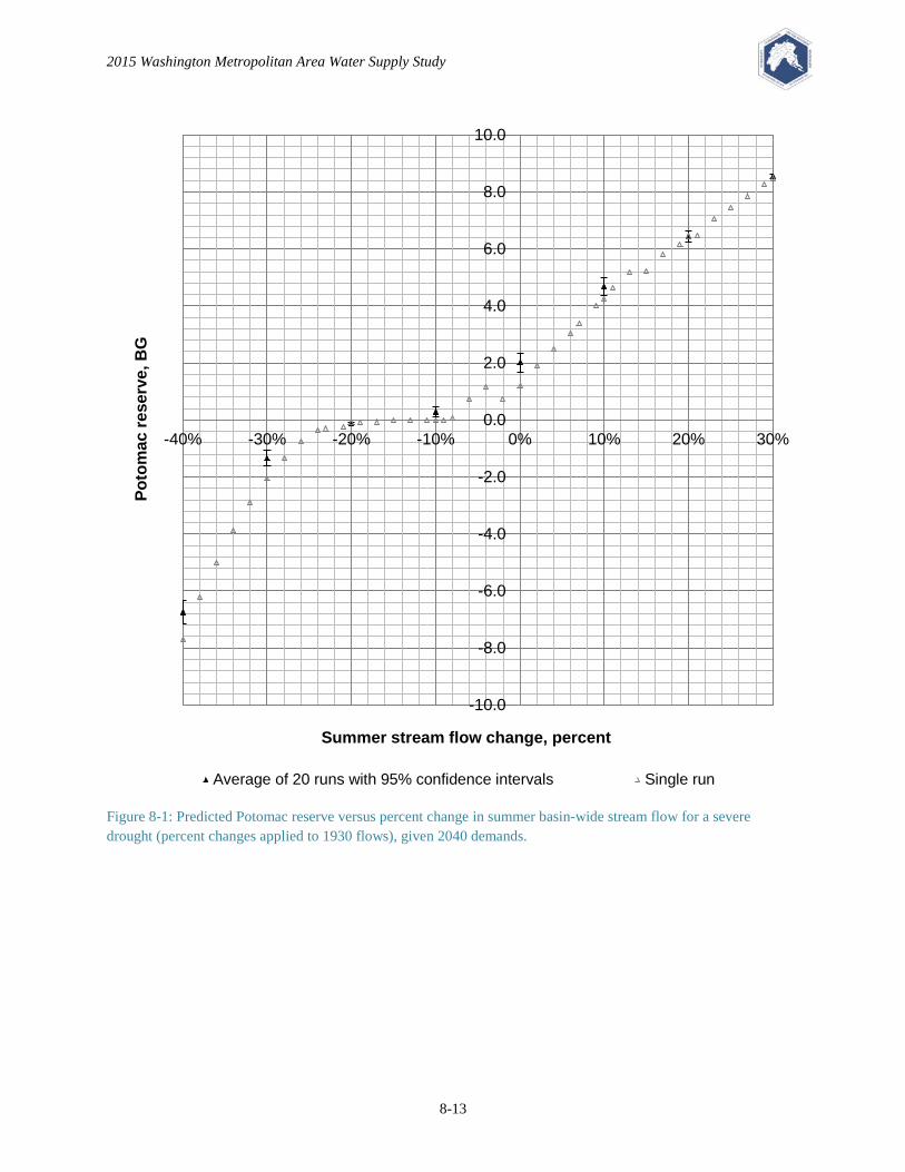
2015 Washington Metropolitan Area Water Supply Study
Figure 8-1: Predicted Potomac reserve versus percent change in summer basin-wide stream flow for a severe drought (percent changes applied to 1930 flows), given 2040 demands.
-10.0
-8.0
-6.0
-4.0
-2.0
0.0
2.0
4.0
6.0
8.0
10.0
-40% -30% -20% -10% 0% 10% 20% 30%
Poto
mac
rese
rve,
BG
Summer stream flow change, percent
Average of 20 runs with 95% confidence intervals Single run
8-13
2015 Washington Metropolitan Area Water Supply Study
8.4.3 Future Use of Climate Change Sensitivity Results
The results presented in Section 8.4 assess the sensitivity of the performance of the current WMA water supply system to changes in long-term average Potomac River basin stream flow. These sensitivities, coupled with the climate response function, Equation (7-2) and Table 7-4, provide a guide for using updated and refined climate projections as they become available. Similarly, these results can help managers interpret research on long-term meteorological and hydrological trends in the Potomac basin and the implications for the WMA water supply system.
Trends in precipitation are difficult to discern because of high inter-annual and inter-decadal variability. National studies have found increasing precipitation and stream flow trends across the United States (Karl and Knight, 1998; Lins and Slack, 1999). A long-term trend of increasing annual precipitation, at a rate of approximately 0.4 inches per decade, has been reported for the Northeast, though this trend may have reversed since 1970 (Hayhoe et al., 2007). For the Potomac River basin, no clear trend in precipitation has emerged from weather observation stations in Maryland (Boesch, 2008); however, significant increases of 5 to 20 percent over the last century have been documented in Pennsylvania (UCS, 2008).
There is some indication that the Potomac River basin is in a transition region, with stream flows increasing to the north and decreasing to the south. An investigation of long-term flow trends was recently completed by the USGS (Rice and Hirsch, 2012). This study analyzed stream flow data from gage stations in the Chesapeake Bay watershed with long-term records for the 1930-2010 period. Several flow statistics were analyzed, both annually and seasonally. The study detected a spatial pattern in its results with many of the mean and low-flow statistics tending to increase at gages above the latitude of 40.25 degrees north, and tending to decrease at gages below this latitude. One of the gages included in the study was the Potomac River at Point of Rocks, Maryland. At Point of Rocks, the study found that annual mean runoff and mean fall, spring, and winter runoff appear to be increasing, but summer mean and annual 7-day minimum flow appear to be decreasing slightly. A more recent study examined the hydrological response of streams along the North American east coast to climate and land use change over the period, 1901-2010 (Yang et al., 2015). Results of this study also indicate that stream flows south of the Potomac basin have been decreasing over the past century, and flows north of the basin have been increasing.
8-14
2015 Washington Metropolitan Area Water Supply Study
9 Summary & Conclusions
The Washington metropolitan area’s cooperative approach to water supply planning and management began in 1982, and it has served the region well for the past 33 years. Coordinated operations during low-flow periods in 1999, 2002, and 2010 provided a reliable supply of water for the residents, businesses, and the federal and local government agencies located in the region. Regular cooperative demand and availability forecasts, conducted using a planning horizon of 20 years or more, provide managers with sufficient warning to ensure that new resources are in place when the need arises. Average annual demand in the WMA, including the City of Rockville, is estimated in the current study to be 486 MGD in year 2015, and is projected to be 529 MGD in 2035, an increase of 9 percent. By the year 2040, WMA demand is forecast to increase by 12 percent from its 2015 level, to 545 MGD.
The WMA has been successful in its efforts towards sustainable demand management. Though the WMA population rose by approximately 18 percent from 1990 to 2015, its water demands have essentially remained constant over that period due to falling per household and per employee use. As discussed in Chapter 3, this decline in unit use is consistent with trends seen throughout the United States. To improve our forecasts of future unit use, a new model was developed for this study which takes into account future reductions in indoor use due to the effects of the U.S. Environmental Protection Agency’s WaterSense program and the U.S. Department of Energy’s Energy Star program, as well as reductions due to the Energy Policy Act of 1992, which was considered in past ICPRB studies. The resulting indoor household use reduction estimate over the 25-year period, 2015-2040, is 25.3 gpd.
Falling unit use rates provide both benefits and challenges for regional water suppliers. Falling unit demand has kept total system demand in check, thereby extending the time period during which current resources can be expected to meet future demands. But reductions in per household and per employee demand have curtailed water supplier revenues and their ability to maintain and augment their infrastructure to serve a growing population (Beecher, 2010). CO-OP water demand forecasts are primarily conducted to assist in long-term planning for water supply storage resources, and for this reason, have often incorporated conservative assumptions to help avoid an under-estimation of future demand. However, demand forecasts may also assist utilities with long-term financial planning, and for this purpose, such conservative assumptions are not appropriate. A probabilistic demand forecast which provided a range of future demand levels and associated probabilities could be used more broadly by water suppliers to inform both resource and financial planning decisions.
Growth in upstream consumptive demand poses another challenge for the region. Summertime upstream consumptive demand has the greatest impact on the WMA water supply system, since WMA demands are at their highest in the summer and flow in the Potomac River tends to be falling. A breakdown of average summer (June, July, and August) upstream consumptive use shows that the four categories of water use with the highest summer consumptive demand are thermoelectric power, public water supply, agricultural irrigation, and self-supplied industry, with public water supply accounting for the greatest forecasted growth. Total summer upstream consumptive use is estimated to be 111 MGD in 2010 and 141 MGD in 2040, an increase of 27 percent.
A final challenge for regional planning is the considerable uncertainty about the impact of climate change on WMA water supplies. This uncertainty stems from the wide range of precipitation projections for the
9-1

2015 Washington Metropolitan Area Water Supply Study
Potomac basin. In the current study, a sensitivity test was conducted to predict the impact on the WMA water supply system performance of precipitation changes of -10 percent to +10 percent and temperature increases of zero to four degrees Fahrenheit. According to a Potomac basin climate response function developed using modeling results from Part 2 of the 2010 demand study, these ranges are associated with changes in average summer stream flow of -38 to +23 percent. Results from the sensitivity test indicate that if future average summer stream flow in the basin rises by 20 percent or more, the current WMA system will have no problem meeting forecasted 2040 demands. If summer flows were to fall by 10 percent or more, with forecasted 2040 demands, model simulations predict that emergency water use restrictions would not be uncommon, during a severe drought system reservoirs would be emptied, and on some days little or no water would flow past Little Falls dam. The sensitivity tests and climate response functions presented here can help managers interpret new climate projections and research on long-term trends as they become available and help determine the implications for the WMA water supply system.
Based on the findings of this study, the following actions are recommended: 1. Regional water suppliers should continue their efforts to identify and evaluate potential new
water supply storage facilities. CO-OP should conduct an evaluation of the relative benefits to the system of a suite of potential options, including new storage facilities and operational changes.
2. CO-OP should continue its development of Watershed Model-based real-time flow forecast tools, to help reduce flow forecast errors and minimize the probability that Potomac River flows will fall below environmental flow targets during droughts.
3. Support should be provided for additional development of ICPRB’s database of Potomac River basin water withdrawals and consumptive use, to provide a sound foundation for basin-wide water supply planning and for the planned basin-wide comprehensive plan.
4. CO-OP should identify methodologies and data needs for conducting a demand forecast in 2020 that would provide a range of future demand levels and associated probabilities, to provide information to the regional suppliers for both resource planning and financial planning purposes.
5. ICPRB and the water suppliers should begin laying the groundwork for a new basin-wide cooperative approach to water supply management by engaging upstream suppliers and state and local agencies through drought exercises, workshops, and task-focused workgroups.
9-2

2015 Washington Metropolitan Area Water Supply Study
10 Literature Cited Ahmed, S. N., K. R. Bencala, and C. L. Schultz. 2010. 2010 Washington Metropolitan Area water supply reliability study, Part 1: Demand and resource availability forecast for the year 2040. Interstate Commission on the Potomac River Basin, ICPRB report 10-01, Rockville, Maryland.
Ahmed, S. N., K.R. Bencala, and C. L. Schultz. 2013. 2010 Washington Metropolitan Area water supply reliability study, Part 2: Potential Impacts of Climate Change. Interstate Commission on the Potomac River Basin, ICPRB report 13-07, Rockville, Maryland.
Ainsworth, E. A. and A. Rogers. 2007. The response of photosynthesis and stomatal conductance to rising [CO2]: mechanisms and environmental interactions. Plant, Cell & Environment, 30: 258–270, doi: 10.1111/j.1365-3040.2007.01641.x
Beecher, J.A. 2010. The conservation conundrum: How declining demand affects water utilities. Journal American Water Works Association, 102(2):78-80.
Boesch, D.F., ed., 2008. Global Warming in the Free State: Comprehensive Assessment of Climate Change Impacts in Maryland. University of Maryland Center for Environmental Science, Cambridge, Maryland.
Brown, C., W. Werick, W. Leger, and D. Fay. 2011. A Decision-Analytic Approach to Managing Climate Risks: Application to the Upper Great Lakes. Journal of the American Water Resources Association, 47 (3):524 -534, doi: 10.1111/j.1752-1688.2011.00552.x
Burns, M. and R. MacArthur. 1996. Sediment Deposition in Jennings Randolph Reservoir, Maryland and West Virginia. Proceedings of the Sixth Federal Interagency Sedimentation Conference. Interagency Advisory Committee on Water Data Subcommittee on Sedimentation, Las Vegas, Nevada, March 10-14.
Butcher, J. B., T. E. Johnson, D. Nover, and S. Sarkar. 2014. Incorporating the effects of increased atmospheric CO2 in watershed model projections of climate change impacts. Journal of Hydrology, 513:322-334.
CDM. 2002. Water Supply Master Planning: Identification of Future FCWA Water Supply Needs. Prepared for Fairfax County Water Authority, Fairfax, Virginia.
Cummins, J., C. Buchanan, C. Haywood, H. Moltz, A. Griggs, R.C. Jones, R. Kraus, N. Hitt, and R.V. Bumgardner. 2010. Potomac Basin Large River Environmental Flow Needs, ICPRB Report No. 10-03, Rockville, Maryland.
De Boer, H. J., E. I. Lammertsma, F. Wagner-Cremer, D. L. Dilcher, M. J. Wassen, and S. C. Dekker. 2011. Climate forcing due to optimization of maximal leaf conductance in subtropical vegetation under rising CO2. Proceedings of the National Academy of Sciences of the United States of America, 108(10): 4041–4046, doi:10.1073/pnas.1100555108
DeOreo, W. B. and P. W. Mayer. 2012. Insights into declining single-family residential water demands. Journal of the American Water Works Association, 104(6):41-42, doi: 10.5942/jawwa.2012.104.0080
10-1
2015 Washington Metropolitan Area Water Supply Study
Dougherty, J. P. 2011. 2002 Mayor’s Message, City of Frederick, Maryland.
Ducnuigeen, J., S. N. Ahmed, K. R. Bencala, H. L. Moltz, A. Nagel, and C. L. Schultz. 2015. Interactive Geospatial Analysis Tool for Estimating Watershed-Scale Consumptive Use: Potomac River Basin Case Study. In: T. Younos, T.E. Parece (eds.), Advances in Watershed Science and Assessment, The Handbook of Environmental Chemistry 33, (pp. 141-169). Springer International Publishing, doi: 10.1007/978-3-319-14212-8_6.
Gilbert, R.O. 1987. Statistical Methods for Environmental Pollution Monitoring. New York, NY: Van Nostrand Reinhold.
Gleckler, P.J., D.E. Taylor, and C. Doutriaux, 2008. Performance Metrics for Climate Models. Journal of Geophysical Research 113:D06114, doi: 10.1029/2007JD008972.
Hagen, E. R., and R.C. Steiner. 1998a. Occoquan Reservoir Watershed: “Natural” Daily Inflow Development. Interstate Commission on the Potomac River Basin, ICPRB report 98-3, Rockville, Maryland.
Hagen, E.R., R.C. Steiner, and J.L. Ducnuigeen. 1998b. Patuxent Reservoirs: “Natural” Daily Inflow Development. Interstate Commission on the Potomac River Basin, ICPRB report 98-4a, Rockville, Maryland.
Hagen, E.R., R.C. Steiner, and J.L. Ducnuigeen. 1998c. Jennings Randolph Reservoir Watershed: “Natural” Daily Inflow Development. Interstate Commission on the Potomac River Basin, ICPRB report 98-5, Rockville, Maryland.
Hagen, E. R., and R.C. Steiner. 1999. Little Seneca Reservoir “Natural” Daily Inflow Development. Interstate Commission on the Potomac River Basin, ICPRB report 99-3, Rockville, Maryland.
Hagen, E.R., and R.C. Steiner. 2000. Year 2000 Twenty-Year Water Demand Forecast and Resource Availability Analysis for the Washington Metropolitan Area. Interstate Commission on the Potomac River Basin, ICPRB report 00-6, Rockville, Maryland.
Holmes, K.J., and R.C. Steiner. 1990. Twenty-Year Water Demand Forecast and Resource Availability Analysis for the Washington Metropolitan Area, Interstate Commission on the Potomac River Basin, ICPRB 90-5, Rockville, Maryland.
Hagen, E.R, K.J. Holmes, J.E. Kiang, and R.C. Steiner. 2005. Benefits of Iterative Water Supply Forecasting in the Washington, D.C. Metropolitan Area. Journal of the American Water Resources Association, 41(6):1417-1430, doi: 10.1111/j.1752-1688.2005.tb03809.x.
Hashimoto, T., J. Stedinger, and D. Loucks. 1982. Reliability, Resiliency, and Vulnerability Criteria For Water Resource System Performance Evaluation. Water Resources Research, 18(1): 14-20, doi: 10.1029/WR018i001p00014.
Hayhoe, Katharine, C.P. Wake, T.G. Huntington, L.F. Luo, M.D. Schwartz, J. Sheffield, E. Wood, B. Anderson, J. Bradbury, A. DeGaetano, T.J. Troy, D. Wolfe, 2007. Past and future changes in climate and
10-2

2015 Washington Metropolitan Area Water Supply Study
hydrological indicators in the US Northeast. Climate Dynamics, 28(4):381-407, doi: 10.1007/s00382-006-0187-8.
Hazen and Sawyer. 2013. Tampa Bay Water - Water Demand Management Plan Final Report. Tampa Bay: Tampa Bay Water. < http://www.tampabaywater.org/documents/conservation/2013_tampabaywater-water-demand-management-plan.pdf>
Horn, M.A., Moore, R.B., Hayes, Laura, and Flanagan, S.M., 2008, Methods for and estimates of 2003 and projected water use in the Seacoast Region, southeastern New Hampshire: U.S. Geological Survey Scientific Investigations Report 2007–5157, 87 p., plus 2 appendixes on CD-ROM (Available at http://pubs.usgs.gov/sir/2007/5157).
Hunter, M., K. Donmoyer, J. Chelius, and G. Naumick. 2011. Declining Residential Water Use Presents Challenges, Opportunities. OpFlow, 37(5):18-20.
Imagine That! 2005. Object oriented software, San Jose, CA., www.imaginethatinc.com.
Kame’enui, A., E.R. Hagen, and J.E. Kiang. 2005. Water Supply Reliability Forecast for the Washington Metropolitan Area Year 2025. Interstate Commission on the Potomac River Basin, ICPRB 05-06, Rockville, Maryland.
Karl, T.R. and R.W. Knight, 1998. Secular trends of precipitation amount, frequency, and intensity in the United States. Bulletin of the American Meteorological Society, 79(2): 231-241.
LaTour, J. K. 1991. Determination of water use in Rockford and Kankakee areas, Illinois: U.S. Geological Survey Water-Resources Investigations Report 90–4166, p 70.
Lins, H.F. and J.R. Slack, 1999. Stream flow trends in the United States. Geophysical Research Letters, 26(2): 227-230, doi: 10.1029/1998GL900291.
Low Flow Allocation Agreement. 1978. Signatories include: the Secretary of the Army for the United States of America, the Governor for the State of Maryland, the Governor for the Commonwealth of Virginia, the Mayor for the District of Columbia, the Chairman of the Washington Suburban Sanitary Commission, and the Chairman of the Fairfax County Water Authority.
McNeil, M., C.D. Whitehead, V. Letschert, and M. Cava. 2008. WaterSense Program: Methodology for National Water Savings Analysis Model Indoor Residential Water Use. Lawrence Berkeley National Laboratory, Berkeley, California.
Mullusky, M. G., S. S. Schwartz, and R. C. Steiner. 1996. 1995 Water Demand Forecast and Resource Availability Analysis for the Washington Metropolitan Area. Interstate Commission on the Potomac River Basin, ICPRB 95-6, Rockville, Maryland.
MWCOG. 2000. Metropolitan Washington Water Supply and Drought Awareness Response Plan: Potomac River System. Metropolitan Washington Council of Governments Board Task Force on Regional Water Supply Issues, Publication number 20703, Washington, D.C.
10-3

2015 Washington Metropolitan Area Water Supply Study
MWCOG. 2009. Round 7.2 Cooperative Forecasting: Employment, Population, and Household Forecasts to 2040 by Traffic Analysis Zone. Metropolitan Washington Council of Governments, Pre-publication version, Washington, D.C.
MWCOG. 2014. Round 8.3 Cooperative Forecasting: Employment, Population, and Household Forecasts to 2040 by Traffic Analysis Zone. Metropolitan Washington Council of Governments, Pre-publication version, Washington, D.C.
NPS. 2008. Letter from D. R. Reidenbach, Northeast Region Regional Director, National Park Service to J. Hoffman, Executive Director, Interstate Commission on the Potomac River Basin, September 16, 2008.
Ocean Surveys, Inc. 1997. Sedimentation Surveys: Phase I– Triadelphia Reservoir: Phase II and III– Rocky Gorge and Little Seneca Lake Reservoirs, Howard and Montgomery Counties, Patuxent River, Maryland, Final Report: OSI Report #95ES047 F, submitted to Washington Suburban Sanitary Commission, WSSC Contract #94101450, Ocean Surveys, Inc., Old Saybrook, Connecticut.
Ortt, R.A., S. VanRyswick, and D. Wells. 2007. Bathymetry and Sediment Accumulation of Tridelphia and Rocky Gorge Reservoirs. Maryland Department of Natural Resources, Maryland Geological Survey, Coastal and Estuarine Geology, File Report No. 07-03, Baltimore, Maryland.
Ortt, R.A., D. V. Wells, and S.VanRyswick. 2011. Bathymetry and Sediment Accumulation of Little Seneca Lake. Maryland Department of Natural Resources, Maryland Geological Survey, Coastal and Estuarine Geology, File Report No. 11-03, Baltimore, Maryland.
Palmer, R.N., J.R. Wright, J.A. Smith, J.L. Cohon, and C.S. ReVelle. 1979. Policy Analysis of Reservoir Operations in the Potomac River Basin, Volume I. Executive Summary. University of Maryland, Water Resources Series Technical Report No. 59, College Park, Maryland.
Palmer, R.N., J.A. Smith, J.L. Cohon, and C.S. ReVelle. 1982. Reservoir management in the Potomac River Basin. Journal of Water Resources Planning and Management, 108(1): 47-66.
Potomac Basin Reporter. 1982. Interstate Commission on the Potomac River Basin, Vol. 38, No. 4, April-May.
Reich, P. B., B. A. Hungate, and Y. Luo. 2006. Carbon-nitrogen interactions in terrestrial ecosystems in response to rising atmospheric carbon dioxide. Annual Review of Ecology, Evolution, and Systematics, 37:611-636, doi: 10.1146/annurev.ecolsys.37.091305.110039.
Rice, K. C., R. M. Hirsch. 2012. Spatial and temporal trends in runoff at long-term streamgages within and near the Chesapeake Bay Watershed: U.S. Geological Survey Scientific Investigations Report 2012–5151, 56 p.
Rockaway, T. D., P. A. Coomes, J. Rivard, and B. Kornstein. 2011. Residential water use trends in North America. Journal of American Water Works Association, 103(2):76-89.
Shaffer, K.H. 2009. Variations in withdrawal, return flow, and consumptive use of water in Ohio and Indiana, with selected data from Wisconsin, 1999–2004: U.S. Geological Survey Scientific Investigations Report 2009–5096, 93 p.
10-4

2015 Washington Metropolitan Area Water Supply Study
Sheer, D.P. 1977. A Perspective on the Washington Metropolitan Area Water Supply Problem. Interstate Commission on the Potomac River Basin, ICPRB M-6, Rockville, Maryland.
Steiner, R.C. 1984. Short-Term Forecasting of Municipal Water Use. Ph.D, diss., The Johns Hopkins University, Baltimore, Maryland.
Steiner, R.C., E.H. Hagen, and J. Ducnuigeen. 2000. Water Supply Demands and Resources Analysis in the Potomac River Basin. Interstate Commission on the Potomac River Basin, ICPRB 00-5, Rockville, Maryland.
UCS. 2008. Climate Change in Pennsylvania Impacts and Solutions for the keystone state: A Climate Impacts Assessment for Pennsylvania. Union of Concerned Scientists. Cambridge, MA.
United States Census Bureau, 2004. Population Division, Information & Research Services Internet Staff. Retrieved August 13, 2004. http://www.census.gov.
USACE. 1963. Potomac River Basin Report. Dept. of the Army, U.S. Army Engineer Division, North Atlantic, Baltimore Basin Studies Branch, Baltimore, Maryland.
USACE. 1975. Metropolitan Washington Area Water Supply Study Report. Department of the Army, North Atlantic Division, Baltimore, Maryland.
USACE. 1983. Metropolitan Washington Area Water Supply Study. Department of the Army, North Atlantic Division, Baltimore, Maryland.
USACE. 1986. Master Manual for Reservoir Regulation in the North Branch Potomac River Basin. U.S. Army Corps of Engineers – Baltimore District, September.
USACE. 2014. Letter from J. R. Jordan, III, Colonel, District Engineer, U.S. Army Corps of Engineers – Baltimore District to C. Haywood, Executive Director, Interstate Commission on the Potomac River Basin, May 15, 2014.
Water Supply Coordination Agreement. 1982. Signatories include: The District Engineer Baltimore District COE for the United States of America, the Chairman of the Fairfax County Water Authority, the General Manager of the Washington Suburban Sanitary Commission, The Mayor of the District of Columbia, General Counsel for the Interstate Commission on the Potomac River Basin.
Ways, H.C. 1993. The Washington Aqueduct 1852-1992. Washington Aqueduct Division, U.S. Army Corps of Engineers, Washington, D.C.
WRF. 2013. Dynamic Reservoir Operations: Managing for Climate Variability and Change. Prepared by D.P. Sheer, M. Rivera, B.A. Wright, and J. Day for the Water Research Foundation. WRF, Denver, CO.
Wu, Y., S. Liu, and O. I. Abdul-Aziz. 2012. Hydrological effects of the increased CO2 and climate change in the Upper Mississippi River Basin using a modified SWAT. Climatic Change, 110(3-4):977-1003, doi: 10.1007/s10584-011-0087-8.
Wurbs, R.A. 1996. Modeling and Analysis of Reservoir System Operations. Upper Saddle River, NJ: Prentice Hall PTR.
10-5

2015 Washington Metropolitan Area Water Supply Study
Yang, Q., H. Tian, M.A.M. Friedrichs, M. Liu, X. Li, and J. Yang. 2015. Hydrological Responses to Climate and Land-Use Changes along the North American East Coast: A 110-Year Historical Reconstruction. Journal of the American Water Resources Association, 51(1): 47-67, DOI: 10.1111/jawr.12232.
10-6