on March 18, 2015http://rsif.royalsocietypublishing.org/Downloaded from

rsif.royalsocietypublishing.org

ResearchCite this article: Friston K, Levin M, Sengupta

B, Pezzulo G. 2015 Knowing one’s place: a

free-energy approach to pattern regulation.

J. R. Soc. Interface 12: 20141383.

http://dx.doi.org/10.1098/rsif.2014.1383

Received: 18 December 2014

Accepted: 24 February 2015

Subject Areas:biocomplexity, systems biology,

biomathematics

Keywords:active inference, morphogenesis, self-assembly,

pattern formation, free energy, random

attractor

Author for correspondence:Michael Levin

e-mail: michael.levin@tufts.edu

& 2015 The Authors. Published by the Royal Society under the terms of the Creative Commons AttributionLicense http://creativecommons.org/licenses/by/4.0/, which permits unrestricted use, provided the originalauthor and source are credited.

Knowing one’s place: a free-energyapproach to pattern regulation

Karl Friston1, Michael Levin2, Biswa Sengupta1 and Giovanni Pezzulo3

1The Wellcome Trust Centre for Neuroimaging, Institute of Neurology, Queen Square, London, UK2Biology Department, Center for Regenerative and Developmental Biology, Tufts University, Medford, USA3Institute of Cognitive Sciences and Technologies, National Research Council, Rome, Italy

Understanding how organisms establish their form during embryogenesis

and regeneration represents a major knowledge gap in biological pattern for-

mation. It has been recently suggested that morphogenesis could be

understood in terms of cellular information processing and the ability of cell

groups to model shape. Here, we offer a proof of principle that self-assembly

is an emergent property of cells that share a common (genetic and epigenetic)

model of organismal form. This behaviour is formulated in terms of variational

free-energy minimization—of the sort that has been used to explain action

and perception in neuroscience. In brief, casting the minimization of thermo-

dynamic free energy in terms of variational free energy allows one to

interpret (the dynamics of) a system as inferring the causes of its inputs—and

acting to resolve uncertainty about those causes. This novel perspective on

the coordination of migration and differentiation of cells suggests an inter-

pretation of genetic codes as parametrizing a generative model—predicting

the signals sensed by cells in the target morphology—and epigenetic processes

as the subsequent inversion of that model. This theoretical formulation

may complement bottom-up strategies—that currently focus on molecular

pathways—with (constructivist) top-down approaches that have proved

themselves in neuroscience and cybernetics.

1. IntroductionOne of the central problems of biology is the origin and control of shape [1–3].

How do cells cooperate to build highly complex three-dimensional structures

during embryogenesis? How are self-limiting growth and remodelling harnessed

for the regeneration of limbs, eyes and brains in animals such as salamanders [4]?

Understanding how to induce specific changes in large-scale shape (not only

gene expression or cell differentiation) is crucial for basic developmental and

evolutionary biology—and is a fundamental requirement for radical advances

in regenerative medicine and synthetic bioengineering [5–9].

Although we now know an enormous amount about the molecular com-

ponents required for patterning [3,10–12], it is currently unclear how the

macromolecular and cellular constituents of a system orchestrate themselves to

generate a specific structure and function [12–16]. Importantly, numerous organ-

isms are able to readjust their pattern to a specific target morphology despite

drastic external perturbations and are able to stop growth and remodelling

when the correct shape is reached [17–19]. It is largely unknown how cell beha-

viours are coordinated to reach correct large-scale morphologies, and how the

system is able to stop when the correct structure is complete. There are very

few constructivist models that show what dynamics are sufficient for complex pat-

terns to arise and be remodelled until a target anatomy results. The current focus

on specific protein pathways has engendered a knowledge gap: high-resolution

genetic data have not, in general, being able to specify what large-scale

shape—or deformations of that shape—can or will occur. An important corollary

is that it is difficult to know how or which of the myriad of low-level components

(genes or proteins) must be tweaked to obtain a specific patterning change [16].

rsif.royalsocietypublishing.orgJ.R.Soc.Interface

12:20141383

2

on March 18, 2015http://rsif.royalsocietypublishing.org/Downloaded from

This holds back progress in the biomedicine of birth defects

and regeneration, which seek to induce the formation of

coherent organs of correct size, shape and orientation—not

merely gene activity profiles or stem-cell differentiation.

In contrast to the near-exclusive pursuit of bottom-up strat-

egies, a complementary approach has recently been suggested

[20,21]. It is possible that top-down models [22–25] could

parsimoniously explain high-level phenomena [26], such as

coordination of cell behaviour towards a specific topological

arrangement, and could provide strategies for exploiting devel-

opmental modularity and pluripotentiality to achieve desired

changes in large-scale shape. Despite the successful use of

goal-seeking models in cybernetics [27], physics [28–30], and

cognitive neuroscience [31,32], these principled approaches

have not been applied to morphogenesis. Here, we explore a

specific application of these ideas, modelling morphogenesis

via an optimality principle.

In this paper, we pursue the notion that morphogenetic self-

organization requires each cell to have an implicit model of its

place in the final morphology [21]—and that self-assembly is

the process of moving to sample local signals that are predicted

by that model. In other words, we consider biologically plaus-

ible solutions to the inverse problem of how cells attain a target

morphology, based upon a forward or generative model of the

signals they should sense after they have attained that form

[16]. In brief, we formalize the solution in terms of an extre-

mum or optimality principle; namely, the minimization of

free energy. This minimization is an inherent aspect of self-

organization at many levels. For example, protein folding

that minimizes thermodynamic free energy [33]. However,

we consider free-energy minimization with a twist: by

re-writing the minimization of thermodynamic free energy in

terms of a variational free energy from information theory,

one can interpret self-organization in a Bayesian sense. Effec-

tively, minimizing variational free energy is equivalent to

maximizing the (Bayesian) evidence for a model that is con-

tained in the signals (data) sampled by a system. This

enables one to talk about self-organization in terms of inference

and probabilistic beliefs that are implicit in its exchange with its

local environment. This perspective is based upon a long his-

tory of theoretical work in the neurosciences that attempts to

formulate action and perception in terms of conscious and

unconscious inference [34–41]. In recent years, the ensuing

variational free-energy principle has been applied to cellular

[42] and pre-biotic self-organization [43]: in which the environ-

ment supplies (sensory) signals to a system’s internal states

which, in turn, inform action on the environment. Both the

changes in internal and active states minimize variational free

energy, resulting in Bayes-optimal perception and action,

respectively. This is known as active inference.Here, we ask whether the same principles can explain

self-assembly in the setting of morphogenesis. This is a par-

ticularly difficult problem because, unlike generic pattern

formation, morphogenesis implies a pre-determined pattern

or form to which an ensemble of cells should converge. How-

ever, from the point of view of any one cell, the remaining

cells constitute external or environmental states that can

only be inferred through intercellular signalling; molecular

or electrochemical [44]. This means that each cell can only

infer its place in the target morphology when all the cells

have reached their target destination—and are releasing the

appropriate (chemotactic) signals. This presents a difficult

chicken and egg (inverse) problem that requires each cell to

differentiate itself from all other cells, so that it can release

signals that enable other cells to differentiate themselves.

One solution to this hard problem of self-assembly is to

assume that every (undifferentiated) cell has the same

model of the cellular ensemble, which it uses to predict the

signals it should encounter at each location in the target

form. At the beginning of morphogenesis, all the cells are

thus identical: they possess the same model and implicit

(stem-cell like) pluripotentiality, and know nothing about

their past locations or their ultimate fate. If each cell then

minimizes variational free energy then it should, in principle,

come to infer its unique place in the ensemble and behave

accordingly. This is guaranteed because the minimum of

variational free energy is obtained when each cell is in a

unique location and has correctly inferred its place. At this

point, it will express the appropriate signals and fulfil the pre-

dictions of all other cells; thereby, maximizing the evidence

for its model of the ensemble (and minimizing the free

energy of the ensemble). This behaviour can be seen as auton-

omous, self-constructing or ‘autopoietic’ in the sense of

Maturana & Varela [45]. In fact, active inference (in many

respects) can be regarded as a formalization of autopoiesis.

In what follows, we present some simple simulations of cell

migration and differentiation that provide a proof of principle

that self-assembly can be understood in these terms. The result-

ing dynamics paint a relatively simple picture, where the

parameters of each cell’s model are genetically encoded—telling

each cell how it should behave (what it should express) if it knew

its place within the ensemble. One can then associate intracellu-

lar signalling—in response to signal receptor activation—with

inferring its place or identity. This inference then leads to the

transcription and release of appropriate molecular signals that

induce intracellular signalling in other cells. This (signalling-

dependent) transcription could be a metaphor for epigenetic

processes. We first briefly review the fundaments of (thermo-

dynamic) free-energy minimization in coupled (random

dynamical) systems and how these can be cast as active (Baye-

sian) inference. We then use this formalism to simulate the

morphogenesis of a simple organism (with a head, body and

tail) to illustrate the emergent behaviour. Finally, we simulate

some experimental perturbations to illustrate the predicted

consequences in terms of regeneration and dysmorphogenesis.

2. Generalized dynamicsWe will consider self-assembly in (weakly mixing ergodic)

random dynamical systems described by stochastic differential

equations of the following form:

_~x ¼ f(~x)þ ~v: (2:1)

Here, the flow of generalized states f(~x) is subject to random

fluctuations ~v. Generalized states ~x ¼ (x, x0, x00, . . . ) comprise

the states per se, their motion, velocity, acceleration and so on.

In essence, these equations specify probability distributions

over paths in generalized coordinates of motion. We can

now use the Helmholtz decomposition (a.k.a. the fundamen-

tal theorem of vector calculus) to express the flow in terms of

a divergence-free component and a curl-free descent on a

scalar Lagrangian L(~x) or Lyapunov function:

f(~x) ¼ (Q� G)rL(~x)

and L(~x) ¼ � ln p(~x):

)(2:2)

external states internal states

s ΠS a ΠA r ΠRy ΠY

Figure 1. Markov blankets and active inference. This schematic illustrates the partition of states into internal states and hidden or external states that areseparated by a Markov blanket—comprising sensory and active states. The internal states can be associated with the intracellular states of a cell, whilesensory states become the surface states of the cell membrane overlying active states (e.g. the actin filaments of the cytoskeleton). The ensuing self-organizationof internal states then corresponds to perception, while action couples internal states back to external states. See table 1 for a definition of variables. (Online versionin colour.)

rsif.royalsocietypublishing.orgJ.R.Soc.Interface

12:20141383

3

on March 18, 2015http://rsif.royalsocietypublishing.org/Downloaded from

This is known as the standard form [46], where the diffusion

tensor G is half the covariance (amplitude) of the random

fluctuations and the matrix Q satisfies r �QrL(~x) ¼ 0.

Because the system is ergodic (and weakly mixing), it

will converge over time to an invariant set of states called a

pullback or random global attractor [47,48]. The associated ergo-dic density p(~x) is the solution to the Fokker–Planck equation

describing the evolution of the probability density over

states. It is straightforward to show that ln p(~x) ¼ �L(~x) is

the solution to the Fokker–Planck equation [49]. In short,

any (weakly mixing ergodic) random dynamical system can

be formulated as a generalized ascent on the log likelihood

of its trajectories. However, this formulation does not dis-

tinguish the states of the self-organizing system from the

states of its local environment. To do this, we have to

consider how the states of a system are separated from its

environment (e.g. heat bath). This calls on the notion of a

Markov blanket.

3. Generalized dynamics and active inferenceA Markov blanket is a set of states that separates two other

sets in a statistical sense. The term was introduced in the

context of Bayesian networks or graphs [50] and refers to

the children of a set (the set of states that are influenced),

its parents (the set of states that influence it) and the other

parents of its children. A Markov blanket induces a partition

of states into internal states and external states that are hidden

(insulated) from the internal (insular) states by the Markov

blanket. For example, the surface of a cell may constitute a

Markov blanket separating intracellular (internal) and extra-

cellular (external) states [43,51]. Statistically speaking,

external states can only be seen vicariously by the internal

states, through the Markov blanket. The Markov blanket

itself can be partitioned into two sets that are, and are not,

children of external states. We will refer to these as surface

or sensory states and actuator or active states, respectively.

Put simply, the existence of a Markov blanket S � A implies

a partition of states into external, sensory, active and internal

states: ~x [ X ¼ C� S� A� R. External states cause sensory

states that influence—but are not influenced by—internal

states, whereas internal states cause active states that influ-

ence—but are not influenced by—external states. Crucially,

the dependencies induced by Markov blankets create a circu-

lar causality that is reminiscent of the action–perception

cycle (figure 1).

We can now consider the dependencies among states

implied by the Markov blanket, in terms of their equations of

motion. In particular, we are interested in the flow of internal

and active states that constitutes the systems response to

sensory signals:

fa(~s, ~a, ~r) ¼ (Qa � Ga)r~aL(~s, ~a, ~r),

fr(~s, ~a, ~r) ¼ (Qr � Gr)r~rL(~s, ~a, ~r)

and L(~s, ~a, ~r) ¼ � ln p(~s, ~a, ~rjm):

9>=>; (3:1)

See [43] for details. This equation is the homologue of

equation (2.2) for internal and active states. It says that their

flow performs a generalized gradient ascent on the marginalergodic density over internal states and their Markov blanket

denoted by m. This means we can describe the (open) system

in terms of a Lagrangian of the system’s states that we will

associate with its thermodynamic free energy—in the setting

of the stochastic thermodynamics of non-equilibrium steady

states [52].

On this point, one could stop and simply marvel at evol-

ution for having selected equations of motion with attractors

that have the intricate forms seen in biotic systems (e.g. pro-

tein folding, morphogenesis and pattern formation). These

attracting forms are described probabilistically in terms of the

thermodynamic free energy, describing the probability over

the systems internal states and Markov blanket. Although we

know this Lagrangian exists, it is practically (almost) imposs-

ible to evaluate its form. However, there is an alternative

formulation of equation (3.1) that allows one to describe

the flow in terms of a probabilistic model of how a system

thinks it should behave. This formulation is based on the

following lemma:

Lemma 3.1 (free energy): for any random dynamical system with aMarkov blanket and Lagrangian L(~x) ¼ � ln p(~c, ~s, ~a, ~rjm), thereis a variational free energy F(~s, ~a, ~r) that describes the flow of

rsif.royalsocietypublishing.orgJ.R.Soc.Interface

12:20141383

4

on March 18, 2015http://rsif.royalsocietypublishing.org/Downloaded from

internal and active states as a generalized descent

fr(~s, ~a, ~r) ¼ (Qr � Gr)r~rF,

fa(~s, ~a, ~r) ¼ (Qa � Ga)r~aF

and F(~s, ~a, ~r) ¼ Eq[L(~x)]�H[q(~cj~r)]

¼ L(~s, ~a, ~r)þDKL[q(~cj~r)jjp(~cj~s, ~a, ~r)]: (3:2)

Proof. See [43]. This lemma says that if one interprets

internal states as parametrizing some arbitrary (variational)

density or Bayesian beliefs q(~cj~r) about external states, then

the dynamics of internal and active states can be described

as a gradient descent on variational free energy. Importantly,

this free energy is a function of states that constitute the

system; namely, the internal states and their Markov blanket.

Variational free energy was introduced by Feynman to

solve difficult integration problems in path integral formu-

lations of quantum physics [53]. This is also the free energy

bound on log model evidence that is used extensively in

approximate Bayesian inference; for example, variational Bayes

and ensemble learning [54–56].

The expressions for variational free energy above highlight

its Bayesian interpretation: the first equality expresses free

energy as the expected Lagrangian (Gibbs energy) minus the

entropy of the variational density. The second equality

shows that variational free energy is the thermodynamic free

energy plus a relative entropy or Kullback–Leibler divergence

[57] between the variational density and the posterior density

over external states. The solution to equation (3.2) implies the

internal states minimize free energy rendering the divergence

zero (by Gibbs inequality). This means the variational free

energy becomes the thermodynamic free energy—and the

variational density becomes the posterior density. In this set-

ting, the thermodynamic free energy is also known as the

log marginal likelihood or log model evidence. In short, the

internal states will appear to engage in Bayesian inference,

effectively inferring the (external) causes of sensory states. Fur-

thermore, the active states are complicit in this inference,

sampling sensory states that maximize model evidence: in

other words, selecting sensations that the system expects.

This is active inference, in which internal states and action mini-

mize free energy—or maximize model evidence—in a way

that is consistent with the good regulator theorem and related

treatments of self-organization [49,58–61].

The variational formulation above speaks directly to two

fundamental observations made at the inception of cyber-

netics; namely, every good regulator is a model of its

environment, and the law of requisite variety [58,62]. The

first observation is endorsed by the fact that variational free

energy is a functional of a probabilistic model of how sensory

states are generated by external states. The law of requisite

variety follows from the fact that the variational density

must be encoded by internal states whose cardinality

equals or exceeds that of the sufficient statistics of the pos-

terior density. This is necessary to eliminate the divergence

between the variational and posterior densities. See [63] for

a closely related discussion of information-based optimality

criteria for control systems. The perspective afforded by the

good regulator theorem highlights the fact that the (open)

system can become the author of its environment. In other

words, it can control external or hidden states through

action—such that they fulfil the predictions of the generative

model. Indeed, as we will see later, the hidden states of the

generative model do not even need to exist—provided their

sensory consequences can be mediated through action. This

is important because it allows one to specify the thermo-

dynamic free energy in terms of a generative model,

thereby specifying sets of attracting states (e.g. target

morphologies) that can have quite complicated forms.

Equipped with this (active inference) formulation, we can

now simulate self-assembly by integrating equation (3.2)

given a (probabilistic generative) model that entails beliefs

about its environment. In other words, we only need to

specify the generative model p(~s, ~a, ~r, ~cjm) and the dynamics

of the environment fc(~c, ~s, ~a) and fs(~c, ~s, ~a) to completely

specify the requisite equations of motion for the system and

its environment. Generally, the model is specified in terms

of nonlinear mappings with additive noise:

s ¼ g(1)(c(1))þ v(1)

c(1) ¼ g(2)(c(2))þ v(2)

..

.

9>>>>=>>>>;

(3:3)

Gaussian assumptions (parametrized by their precision

or inverse variance) about the random fluctuations ~v pre-

scribe the likelihood and priors over external states that

define the Lagrangian or generative model

L(~x) ¼ � ln p(~s, ~a, ~r, ~cjm)

¼ � ln p(~s, ~a, ~rj~c(1))� ln p(~c

(1)j~c(2)) . . .

p(~s, ~a, ~rj~c(1)) ¼ N (g(1)(c(1)), P(1))

p( ~c(1)j~c(2)

) ¼ N (g(2)(c(2)), P(2))

..

.

9>>>>>>>>>>>=>>>>>>>>>>>;

(3:4)

where P(i) correspond to the precision or inverse variance of

the random fluctuations. In what follows, we integrated

equation (3.2) using the Matlab routine spm_ADEM.m in

the SPM academic freeware.1 This scheme uses the Laplace

assumption q(~cj~r) ¼ N (~r,�r~r~rL(~s, ~a, ~r, ~r)) and associates

divergence-free flow within generalized motion

QrrL(~r) ¼ D~r ¼ (r0, r00, . . . ). The resulting scheme can be

regarded as a generalized Bayesian filter, in which the

internal states become the expected values of the external

or hidden states, see [64] for details. This scheme has been

used in several papers to simulate active inference in the

neurosciences. In what follows, we use it to simulate self-

assembly—and how this illuminates the role of genetics

and epigenetics in morphogenesis. These simulations are

offered as a proof of principle that the above scheme provides

a sufficient explanation for (simple) self-assembly.

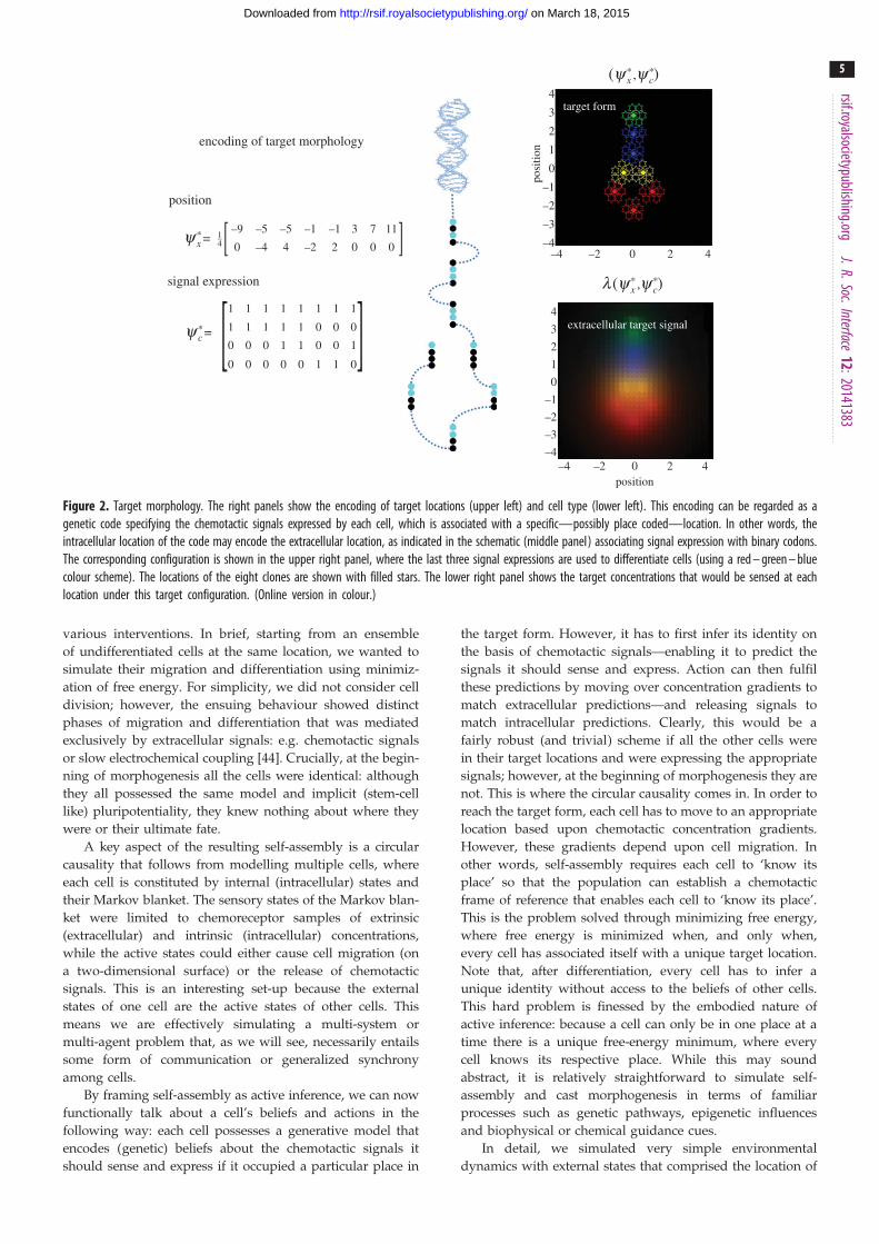
4. Simulating self-assemblyWe simulated morphogenesis given a target morphology

specified in terms of the location and differentiation of

eight clones or cells shown in figure 2 (a simple form with

a head, body and tail). Here, we focus on the migration

and differentiation of each clone prior to subsequent prolifer-

ation (filled cells in the upper right panel of figure 2). We

deliberately stripped down the problem to its bare essentials

to illustrate the nature of the dynamics, which will be used in

the final section to make predictions about the results of

encoding of target morphology

position

signal expression

–9 –5 –5 –1 –1 3 7 11

0 –4 4 –2 2

1 1 1 1 1 1 1 1 4

3

2

1

0

–1

–2

–3

–4–4 –2 0

position

posi

tion

extracellular target signal

target form

2 4

4

3

2

1

0

–1

–2

–3

–4–4 –2 0 2 4

1 1 1 1 1 0 0 0

0 0 0 1 1 0 0 1

0 0 0 0 0 1 1 0

0 0 0y *

x =

(y *x ,y *

c)

l (y *x ,y *

c)

y *c =

14–

Figure 2. Target morphology. The right panels show the encoding of target locations (upper left) and cell type (lower left). This encoding can be regarded as agenetic code specifying the chemotactic signals expressed by each cell, which is associated with a specific—possibly place coded—location. In other words, theintracellular location of the code may encode the extracellular location, as indicated in the schematic (middle panel) associating signal expression with binary codons.The corresponding configuration is shown in the upper right panel, where the last three signal expressions are used to differentiate cells (using a red – green – bluecolour scheme). The locations of the eight clones are shown with filled stars. The lower right panel shows the target concentrations that would be sensed at eachlocation under this target configuration. (Online version in colour.)

rsif.royalsocietypublishing.orgJ.R.Soc.Interface

12:20141383

5

on March 18, 2015http://rsif.royalsocietypublishing.org/Downloaded from

various interventions. In brief, starting from an ensemble

of undifferentiated cells at the same location, we wanted to

simulate their migration and differentiation using minimiz-

ation of free energy. For simplicity, we did not consider cell

division; however, the ensuing behaviour showed distinct

phases of migration and differentiation that was mediated

exclusively by extracellular signals: e.g. chemotactic signals

or slow electrochemical coupling [44]. Crucially, at the begin-

ning of morphogenesis all the cells were identical: although

they all possessed the same model and implicit (stem-cell

like) pluripotentiality, they knew nothing about where they

were or their ultimate fate.

A key aspect of the resulting self-assembly is a circular

causality that follows from modelling multiple cells, where

each cell is constituted by internal (intracellular) states and

their Markov blanket. The sensory states of the Markov blan-

ket were limited to chemoreceptor samples of extrinsic

(extracellular) and intrinsic (intracellular) concentrations,

while the active states could either cause cell migration (on

a two-dimensional surface) or the release of chemotactic

signals. This is an interesting set-up because the external

states of one cell are the active states of other cells. This

means we are effectively simulating a multi-system or

multi-agent problem that, as we will see, necessarily entails

some form of communication or generalized synchrony

among cells.

By framing self-assembly as active inference, we can now

functionally talk about a cell’s beliefs and actions in the

following way: each cell possesses a generative model that

encodes (genetic) beliefs about the chemotactic signals it

should sense and express if it occupied a particular place in

the target form. However, it has to first infer its identity on

the basis of chemotactic signals—enabling it to predict the

signals it should sense and express. Action can then fulfil

these predictions by moving over concentration gradients to

match extracellular predictions—and releasing signals to

match intracellular predictions. Clearly, this would be a

fairly robust (and trivial) scheme if all the other cells were

in their target locations and were expressing the appropriate

signals; however, at the beginning of morphogenesis they are

not. This is where the circular causality comes in. In order to

reach the target form, each cell has to move to an appropriate

location based upon chemotactic concentration gradients.

However, these gradients depend upon cell migration. In

other words, self-assembly requires each cell to ‘know its

place’ so that the population can establish a chemotactic

frame of reference that enables each cell to ‘know its place’.

This is the problem solved through minimizing free energy,

where free energy is minimized when, and only when,

every cell has associated itself with a unique target location.

Note that, after differentiation, every cell has to infer a

unique identity without access to the beliefs of other cells.

This hard problem is finessed by the embodied nature of

active inference: because a cell can only be in one place at a

time there is a unique free-energy minimum, where every

cell knows its respective place. While this may sound

abstract, it is relatively straightforward to simulate self-

assembly and cast morphogenesis in terms of familiar

processes such as genetic pathways, epigenetic influences

and biophysical or chemical guidance cues.

In detail, we simulated very simple environmental

dynamics with external states that comprised the location of

Table 1. Definitions of the tuple (V, C, S, A, L, p, q) underlying active inference.

a sample space V or non-empty set from which random fluctuations or outcomes v [ V are drawn

external states C : C� A�V! R—hidden states of the world that cause sensory states and depend on action

sensory states S: C� A�V! R—signals that constitute a probabilistic mapping from action and external states

active states A: S � R�V! R—action that depends on sensory and internal states

internal states R: R� S �V! R—representational states that cause action and depend on sensory states

ergodic density p( ~c, ~s, ~a, ~rjm)—a probability density function over external ~c [ C, sensory ~s [ S, active ~a [ A and internal states ~r [ R for a

Markov blanket denoted by m

variational density q( ~cj~r)—an arbitrary probability density function over external states that is parametrized by internal states

rsif.royalsocietypublishing.orgJ.R.Soc.Interface

12:20141383

6

on March 18, 2015http://rsif.royalsocietypublishing.org/Downloaded from

each cell cx [ R2 and its release of four chemotactic signals

cc [ R4, which were the corresponding active states of each

cell. More realistic simulations would model cell migration

and signalling as a function of action; however, we will

assume action is sufficiently fast to use the adiabatic approxi-

mation c � a: i.e. the solution to t _c ¼ a� c: t� 0. Sensory

states corresponded to chemotactic concentrations of intra-

cellular, exogenous and extracellular signals. Here we

assume the existence of exogenous (linear) concentration

gradients, which we will relax later

s ¼scsxsl

24

35 ¼ cc

cxl(cx, cc)

24

35þ v : (4:1)

The signal receptor noise was set at very low levels with a

log precision of 216. The function l(cx, cc) returns extra-

cellular signal levels generated by all cells assuming a

monoexponential spatial decay of concentration for each of

the signals: where, for the ith cell

li(cx, cc) ¼ t �X

jccj � exp (jcxi � cxjj) (4:2)

where, t [ [0, 1] is developmental time and models a linear

increase in sensitivity to extracellular signals (e.g. the progress-

ive expression of cell surface receptors over time). Finally, each

cell is assumed to have the same generative model specified in

terms of the mapping from hidden states to sensations

g(c) ¼c�cc�xl�

264

375s(c),

l� ¼ l(c�x, c�c )

and s(ci) ¼exp (ci)Pi exp (ci)

9>>>>>>>>>=>>>>>>>>>;

(4:3)

where, the matrices (c�x, c�c ) correspond to target locations

and the combinations of the four signals expressed at these

locations, respectively. The (softmax) function of hidden

states s(c) returns expectations about the identity of each

cell. These expectations enable the cell to predict which chemo-

tactic signals it should express and sense. We assumed (zero

mean) Gaussian priors over the hidden states with a small pre-

cision P(2) (with a log precision of minus two). This means that

the cells have prior beliefs that they have a high expectation of

being a particular clone but they do not know which clone they

only belong to. This form of prior is ubiquitous in generative

models of sparse causes (e.g. [65]). The resulting model is extre-

mely simple and has no hierarchical structure, enabling us to

drop the superscripts of equation (3.2).

This generative model or Lagrangian produces remarkably

simple dynamics for internal and external states (suppressing

higher order terms and using A � B W ATB):

fr(~s, ~a, ~r) ¼ (Qr � Gr)r~rF ¼ D~r�r~r~1 �P(1)~1�P(2)~r

fa(~s, ~a, ~r) ¼ (Qa � Ga)r~aF ¼ D~a�r~a~s �P(1)~1

)

_~ac ¼ D~ac �P(1)c ~1c þP

(1)l ~1l

_~ax ¼ D~ax �rx~sx �P(1)x ~1x þrx~sl �P(1)

l ~1l

1 ¼1c

1x

1l

264

375 ¼

sc � c�cs(r)

sx � c�xs(r)

sl � l�s(r)

264

375

9>>>>>>>>>>>>>>>>>=>>>>>>>>>>>>>>>>>;

(4:4)

where, 1 ¼ s� g(r) is the prediction error at the level of chemo-

tactic signal receptors whose gradients are rx~s ¼ @~s=@cx ¼@~s=@ax. The signal precision P(1) had a log precision of two,

where the precisions over (generalized) motion modelled

random fluctuations with a Gaussian autocorrelation function

of one. These equations have some straightforward interpret-

ations: the internal states organize themselves to minimize

(precision weighted) prediction error based upon predictions.

These predictions are weighted mixtures of target locations

and concentrations encoded by (c�x, c�c ). If we associate this

encoding with a genetic code, then its transcription into

predictions can be associated with epigenetic processes (i.e.

intracellular signalling-dependent transcription). Figure 2

illustrates this graphically using the target morphology

assumed for the simulations. Here, different segments of the

target form are associated with four cell types, defined in

terms of the combination of signals expressed.

The updates for action are even simpler. Active states

control the expression of chemotactic signals and cell

migration. Signal expression simply attempts to close the

gap between the predicted and detected signals, while

migration is driven by local concentration gradients sensed

by the cell. It is interesting to note that these gradients require

a distribution of receptors over a spatially extensive surface or

sensory epithelia, which is characteristic of living organisms.

Furthermore, it requires the spatial scale of cells to be non-

trivial in relation to chemotactic gradients; although see

[66] for a discussion of active sampling in this context.

Heuristically speaking, the cell moves to fulfil its expectations

about the signals it thinks it should encounter, while expres-

sing the signals associated with its current beliefs about its

place in the target ensemble.

Figure 3 shows the resulting self-assembly using the

target morphology shown in figure 2. These simulations

5

3.0

2.5

2.0

1.5

1.0

0.5

0

–0.5

–1.0

–1.5

–420 8

7

6

5

4

3

2

1

–400

–380

–360

–340

2.5

2.0

1.5

1.0

0.5

0

–0.5

–1.0

–1.5

–2.0 –4

–3

–2

–1

0

1

2

3

4

–4

–3

–2

–1

0

1

2

3

4

10 15time

expectations

free energy solutionsoftmax expectations

free

ene

rgy

cell

action morphogenesis

20 25 30

5 54321 6 7 8 –4 –2 0 2 410 15time cell location

20 25 30

5 10 15time

20 25 30 5 100 15time

loca

tion

20 25 30 35

Figure 3. Self-assembly. This figure shows the results of a simulation in terms of the solution or trajectory implied by active inference. This simulation used a locallinear approximation to integrate the generalized descent on free energy (equation (4.3)) in 32 time steps, using the target morphology for eight cells in figure 2.Each time step can be thought of as modelling migration and differentiation over several minutes. The upper panels show the time courses of expectations aboutcell identity (left), the associated active states mediating migration and signal expression (middle) and the resulting trajectories; projected onto the first (vertical)direction—and colour-coded to show differentiation. These trajectories progressively minimize free energy (lower left panel), resulting in expectations that establisha relatively unique differentiation of the ensemble (lower middle panel). This panel shows the softmax function of expectations for each of eight cells, which can beinterpreted as the posterior beliefs that each cell (column) occupies a particular place in the ensemble (rows). The columns have been reordered so that themaximum in each row lies along the leading diagonal. The lower right panel shows the ensuing configuration using the same format as figure 2. Here, the trajectoryis shown in small circles ( for each time step). The insert corresponds to the target configuration. (Online version in colour.)

rsif.royalsocietypublishing.orgJ.R.Soc.Interface

12:20141383

7

on March 18, 2015http://rsif.royalsocietypublishing.org/Downloaded from

used 32 time steps (each corresponding to several minutes).

The resulting trajectories show several interesting features.

First, there is a rapid dispersion and migration of the cells

to their target locations, followed by a differentiation into

the respective cell types (at about the eighth time step).

This migration and differentiation is accompanied by a pro-

found reduction in free energy—as the solution converges

towards the target configuration. Note the initial increase in

free energy as cells disperse a bit too quickly on the first iter-

ation (as often seen with nonlinear generative models). The

free energy here is the free energy of the ensemble or the

sum of the free energy of each cell (because the variational

and posterior densities are conditionally independent given

sensory signals). All the cells started at the same location

and with undifferentiated expectations about their fate

(using small random expectations with a log precision of

minus four). In this example, the self-assembly is not perfect

but reproduces the overall form and differentiation into a

head, body and tail cell types. We terminated the simulation

prematurely to illustrate the partial resolution of uncertainty

about cellular identity implicit in the expectations encoded

by the internal states. These are shown in the lower middle

panel of figure 3 for all cells (after application of the softmax

function) and can be interpreted as a confusion matrix. The

off-diagonal block structure of this confusion matrix shows

that, as one might expect, there is a mild confusion between

head and body cells, and between body and tail cells (but not

between head and tail cells). This confusion resolves after

continued differentiation (results not shown).

These results are compelling in the sense that they show

cells can resolve ambiguity about their fate, even when that

resolution depends upon the context established by other

(equally ambiguous) cells. Subsequent work will increase

these models’ biological realism by associating various quan-

tities with intracellular signalling and transcription, to enable

testing of specific predictions about the outcomes of various

experimental interventions. To illustrate the potential of this

sort of modelling, we conclude with a brief simulation of

regeneration and dysmorphogenesis to illustrate the sorts

of behaviour the simple system above can exhibit.

5. Simulating regeneration anddysmorphogenesis

Real biological tissues demonstrate remarkable self-repair

and dynamic reconfiguration. For example, planarian regen-

eration provides a fascinating model of reconfiguration

following removal of body parts or complete bisection

(reviewed in [4]); early embryos of many species are likewise

–4–4

–3

–2

–1

0

1

2

3

4

–4

–3

–2

–1

0

1

2

3

4

–2 00 5 10 15 20 25 30 35location

loca

tion

time

morphogenesis

regeneration of head

–4

–3

–2

–1

0

1

2

3

4

0 5 10 15 20 25 30 35

loca

tion

time

morphogenesis

regeneration of tail

2 4

Figure 4. Simulating regeneration. This figure reports simulated interventions that induce dynamic reorganization. The left panels show the normal self-assembly ofeight cells or clones over iterations using the format of the previous figures (with a veridical generative model). The right panels show the development of theensemble after it has been split into two (by the dashed line) and duplicated. The upper panels show the fate of the cells that were destined to be the tail, whereasthe lower panels show the corresponding development of cells destined to be the head. Both of these (split embryo) clones dynamically reconfigure themselves toproduce the target morphology, although the head cells take slightly longer before it ultimately converges (results not shown). (Online version in colour.)

rsif.royalsocietypublishing.orgJ.R.Soc.Interface

12:20141383

8

on March 18, 2015http://rsif.royalsocietypublishing.org/Downloaded from

regulative and fully remodel following bisection. To illustrate

this sort of behaviour, we simulated morphogenesis for eight

time steps and then cut the partially differentiated embryo

into two. We then simulated cell division by replicating the

cells in each half (retaining their locations and partial differ-

entiation) and continued integrating the morphogenetic

scheme for each part separately.

The left panels of figure 4 shows normal morphogenesis

over eight time steps, while the upper row shows the sub-

sequent development of the progenitor tail cells over 32

iterations. This effectively simulates the regeneration of a

head. The complementary development of the head cells

can be seen in the lower panels. One can see that the cells

(that were originally destined to become tail and head cells)

undergo a slight dedifferentiation before recovering to pro-

duce the target morphology. In this example, the head of

the split embryo takes slightly longer to attain the final

form. This example illustrates the pluripotential nature of

the cells and the ability of self-assembly to recover from

fairly drastic interventions.

To illustrate dysmorphogenesis (e.g. induced birth

defects), we repeated the above simulations while changing

the influence of extracellular signals—without changing the

generative model (genetic and epigenetic processes). Figure 5

shows a variety of abnormal forms when changing the levels

of (or sensitivity to) exogenous, intracellular and extracellular

signals. For example, when the sensitivity to exogenous gradi-

ents is suppressed, the cells think they have not migrated

sufficiently to differentiate and remain confused about their

identity. Conversely, if we increase the sensitivity to the verti-

cal gradient, the cells migrate over smaller vertical distances

resulting in a vertical compression of the final form. Doubling

the sensitivity to intracellular signals causes a failure of

migration and differentiation and generalized atrophy. More

selective interventions produce a dysmorphogenesis of various

segments of the target morphology: reducing sensitivity to

the second chemotactic signal—that is expressed by head

cells—reduces the size of the head. Similarly, reducing sensi-

tivity to the third signal induces a selective failure of body

cells to differentiate. These simulations are not meant to be

exhaustive but illustrate the predictions one could make fol-

lowing experimental manipulations (e.g. pharmacological) of

intercellular signalling.

6. ConclusionIn summary, we have introduced a variational (free energy)

formulation of ergodic systems and have established a

proof of principle (through simulations) that this formulation

can explain a simple form of self-assembly towards a specific

pattern. We have framed this in terms of morphogenesis,

relating the generative model implicit in any self-organizing

system to genetic and epigenetic processes. There are clearly

many areas for subsequent expansion of this work; for

example, cell division and neoplasia: see [67]—and the vast

knowledge accumulated about the molecular biology and

biophysics of morphogenesis. Furthermore, we have only

considered generative models that have a fixed point attrac-

tor. In future work, it would be interesting to include

equations of motion in the generative model, such that certain

cell types could express fast dynamics and generate dynamic

behaviours (like pulsation) following differentiation. Finally,

future work should explore whether and how the self-

organization and autopoietic dynamics that we demonstrated

in the morphogenetic domain generalize to larger-scale

gradient

Sx = ·yx12–

Sc2 = ·yc214– Sc3 = ·yc3

14–

Sx1 = 2·yx1

Ss = 2·ys

gradient

dysmorphogenesis

target

intrinsic extrinsicextrinsic

Figure 5. Perturbing self-assembly. The upper right and left panels show deviations from the target configuration when the self-assembly is confounded bychanging the concentration of (or sensitivity to) exogenous gradients. The first intervention illustrates a failure of migration and differentiation that resultsfrom non-specific suppression of exogenous signals, while selectively increasing the vertical gradient produces compression along the corresponding direction.More exotic forms of dysmorphogenesis result when decreasing the intracellular (intrinsic: lower left panel) and extracellular (extrinsic: lower right panels) receptorsensitivities. (Online version in colour.)

rsif.royalsocietypublishing.orgJ.R.Soc.Interface

12:20141383

9

on March 18, 2015http://rsif.royalsocietypublishing.org/Downloaded from

phenomena such as brains and societies, as has been

variously proposed [45,68].

The premise underlying active inference is based upon a

variational free energy that is distinct from thermodynamic

free energy in physics. In fact, strictly speaking, the formalism

used in this paper ‘sits on top of’ classical physics. This is

because we only make one assumption; namely, that the

world can be described as a random dynamical system.

Everything follows from this, using standard results from

probability theory. So how does variational free energy

relate to thermodynamic free energy? If we adopt the

models assumed by statistical thermodynamics (e.g. canoni-

cal ensembles of microstates), then variational free-energy

minimization should (and does) explain classical mechanics

(e.g. [69,70]). In a similar vein, one might hope that there is

a close connection with generalizations of thermodynamic

free energy to far-from-equilibrium systems [71] and

non-equilibrium steady state (e.g. [52,72]). This might be

important in connecting variational and thermodynamic

descriptions. For example, can one cast external states as a

thermal reservoir and internal states as a driven system? In

driven systems—with a continuous absorption of work fol-

lowed by dissipation—the reliability or probability of such

exchange processes might be measured by the variational

free-energy, so that stable structures are formed at its

minima [73]. However, questions of this sort remain an

outstanding challenge.

Our simulations rest on several simplifying assumptions,

such as what is coded in the cells, the (place-coded) nature of

the target location, and the specifics of cell–cell communication.

It is important to note that the framework does not depend

explicitly on these assumptions—and extending the model to

include more detailed and realistic descriptions of genetic

coding and signalling is an open challenge. A potentially excit-

ing application of these schemes is their use as observation

models of real data. This would enable the model parameters

to be estimated, and indeed the form of the model to be

identified using model comparison. There is an established pro-

cedure for fitting models of time-series data—of the sort

considered in this paper—that has been developed for the analy-

sis of neuronal networks. This is called dynamic causal modelling[74,75] and uses exactly the same free-energy minimization

described above. Although the nature of neuronal network

and morphogenetic models may appear different, formally

they are very similar: neuronal connectivity translates into

kinetic rate constants (e.g. as controlled by the precisions

above) and neuronal activity translates to the concentration or

expression of various intracellular and extracellular signals. In

principle, the application of dynamic causal modelling to

empirical measurements of morphogenesis should provide a

way to test specific hypotheses through Bayesian model com-

parison [76] and ground the above sort of modelling in a

quantitative and empirical manner. It should also be pointed

out that is now clear that even non-neuronal cells possess

many of the same ion channel- and electrical synapse-based

mechanisms as do neurons and use them for pattern formation

and repair [77–82]. This suggests the possibility that significant

commonalities may exist between the dynamics of neural net-

works and of bioelectric signalling networks that control shape

determination [20,21,83].

The example in this paper uses a fairly arbitrary genera-

tive model. For example, the choice of four signals was

rsif.royalsocietypublishing.orgJ.R.Soc.Interface

12:20141383

10

on March 18, 2015http://rsif.royalsocietypublishing.org/Downloaded from

largely aesthetic—to draw a parallel with DNA codons: the

first signal is expressed by all cells and is primarily concerned

with the intercellular spacing. The remaining three signals

provide for eight combinations or differentiated cell types

(although we have only illustrated four). One might also

ask about the motivation for using an exogenous gradient.

This is not a necessary component of the scheme; however,

our simulations suggest that it underwrites a more robust

solution for larger ensembles (with more than four clones).

Furthermore, it ensures that the orientation of the target

morphology is specified in relation to an extrinsic frame of

reference. Having said this, introducing a hierarchical

aspect to the generative model may be a more graceful way

to model real morphogenesis at different spatial scales.

We have hypothesized that the parameters of each cell’s

model are genetically encoded. Another intriguing possibility

is that the cells learn some model parameters during epigen-

esis and growth through selective expression of a fixed code.

In other words, during growth, each cell might acquire (or

adjust) the parameters of its generative model such that the

target morphology emerges during epigenesis. The organism

as a whole may therefore exhibit a self-modelling process—

where they are essentially modelling their own growth

process. A useful analogy here is self-modelling robots,

which learn models of their own structure (e.g. their body

morphology) and use those models to predict the sensory

consequences of movement—and maintain their integrity or

recover from injuries [84]. In computational neuroscience

and machine learning, various methods have been proposed

for this form of (structure) learning [85]. Technically, the

difference between learning and inference pertains to the

optimization of parameters and expected states with respect

to model evidence (i.e. free energy). We have focused on

inferring (hidden) states in this paper, as opposed to par-

ameters (like log precisions). It may be worth concluding

that although aspects of the target morphology are geneti-

cally encoded (in the parameters of the generative models);

epigenetic processes (active inference) are indispensable for

patterning. Indeed, it is possible to permanently alter the

regenerative target morphology in some species; for example,

perpetually two-headed planaria can be created by a brief

modification of the electric synapses [44,86].

Finally, we have not considered the modelling of different

phases of development or hierarchical extensions of the basic

scheme. Having said this, the variational formulation offered

here provides an interesting perspective on morphogenesis

that allows one to talk about the beliefs and behaviour of

cells that have to (collectively) solve the most difficult of infer-

ence problems as they navigate in autopoietic frame of

reference. It is likely that this is just a first step on an impor-

tant roadmap to formalize the notion of belief and

information-processing in cells towards the efficient, top-

down control of pattern formation for regenerative medicine

and synthetic bioengineering applications. Perhaps the last

word on this spatial inverse problem should go to Helmholtz

[35], p. 384

Each movement we make by which we alter the appearance ofobjects should be thought of as an experiment designed to testwhether we have understood correctly the invariant relations ofthe phenomena before us, that is, their existence in definitespatial relations.

Acknowledgements. We would like to thank Daniel Lobo for helpfulguidance and comments on this work.

Funding statement. We are grateful for the support of the Wellcome Trust(K.F. and B.S. are funded by a Wellcome Trust Principal ResearchFellowship Ref: 088130/Z/09/Z), the G. Harold and Leila Y. MathersCharitable and Templeton World Charity Foundations (M.L.), theEuropean Community’s Seventh Framework Programme (G.P. isfunded by FP7/2007-2013 project Goal-Leaders FP7-ICT-270108) andthe HFSP (G.P. is funded by grant no: RGY0088/2014).

Endnote1http://www.fil.ion.ucl.ac.uk/spm/. The simulations in this papercan be reproduced by downloading the SPM freeware and typingDEM to access the DEM Toolbox graphical user interface. The requi-site routines can be examined and invoked with the morphogenesis

button. Annotated Matlab code provides details for performingsimulations with different target morphologies—or differentchemotactic signalling.

References

1. Turing AM. 1952 The chemical basis ofmorphogenesis. Phil. Trans. R. Soc. Lond. B 237,37 – 72. (doi:10.1098/rstb.1952.0012)

2. Iskratsch T, Wolfenson H, Sheetz MP. 2014Appreciating force and shape—the rise ofmechanotransduction in cell biology. Nat. Rev. Mol.Cell Biol. 15. 825 – 833. (doi:10.1038/nrm3903)

3. Sandersius SA, Weijer CJ, Newman TJ. 2011 Emergentcell and tissue dynamics from subcellular modelingof active biomechanical processes. Phys. Biol. 8,045007. (doi:10.1088/1478-3975/8/4/045007)

4. Mustard J, Levin M. 2014 Bioelectrical mechanismsfor programming growth and form: tamingphysiological networks for soft body robotics. SoftRobot. 1, 169 – 191. (doi:10.1089/soro.2014.0011)

5. Levin M. 2011 The wisdom of the body: futuretechniques and approaches to morphogenetic fieldsin regenerative medicine, developmental biology

and cancer. Regener. Med. 6, 667 – 673. (doi:10.2217/rme.11.69)

6. Davies JA. 2008 Synthetic morphology: prospects forengineered, self-constructing anatomies. J. Anat.212, 707 – 719. (doi:10.1111/j.1469-7580.2008.00896.x)

7. Doursat R, Sanchez C. 2014 Growing fine-grainedmulticellular robots. Soft Robot. 1, 110 – 121.(doi:10.1089/soro.2014.0014)

8. Doursat R, Sayama H, Michel O. 2013 A review ofmorphogenetic engineering. Nat. Comput. 12,517 – 535. (doi:10.1007/s11047-013-9398-1)

9. Lander AD. 2011 Pattern, growth, andcontrol. Cell 144, 955 – 969. (doi:10.1016/j.cell.2011.03.009)

10. Davidson EH. 2009 Network design principles fromthe sea urchin embryo. Curr. Opin. Genet. Dev. 19,535 – 540. (doi:10.1016/j.gde.2009.10.007)

11. Woolf NJ, Priel A, Tuszynski JA, Woolf NJ, Priel A,Tuszynski JA. 2009 Nanocarriers and intracellulartransport: moving along the cytoskeletal matrix.In Nanoneuroscience: structural andfunctional roles of the neuronal cytoskeleton inhealth and disease (eds NJ Woolf, A Priel,JA Tuszynski), pp. 129 – 176. Berlin, Germany:Springer.

12. Wolkenhauer O, Ullah M, Kolch W, Cho KH. 2004Modeling and simulation of intracellular dynamics:choosing an appropriate framework. IEEE Trans.Nanobiosci. 3, 200 – 207. (doi:10.1109/TNB.2004.833694)

13. Cademartiri L, Bishop KJ, Snyder PW, Ozin GA. 2012Using shape for self-assembly. Phil. Trans. R. Soc. A370, 2824 – 2847. (doi:10.1098/rsta.2011.0254)

14. Lutolf MP, Hubbell JA. 2005 Synthetic biomaterialsas instructive extracellular microenvironments for

rsif.royalsocietypublishing.orgJ.R.Soc.Interface

12:20141383

11

on March 18, 2015http://rsif.royalsocietypublishing.org/Downloaded from

morphogenesis in tissue engineering. Nat.Biotechnol. 23, 47 – 55. (doi:10.1038/nbt1055)

15. Foty RA, Steinberg MS. 2005 The differentialadhesion hypothesis: a direct evaluation. Dev. Biol.278, 255 – 263. (doi:10.1016/j.ydbio.2004.11.012)

16. Lobo D, Solano M, Bubenik GA, Levin M. 2014 Alinear-encoding model explains the variability of thetarget morphology in regeneration. J. R. Soc.Interface 11, 20130918. (doi:10.1098/rsif.2013.0918)

17. Vandenberg LN, Adams DS, Levin M. 2012Normalized shape and location of perturbedcraniofacial structures in the Xenopus tadpole revealan innate ability to achieve correct morphology.Dev. Dyn. 241, 863 – 878. (doi:10.1002/dvdy.23770)

18. Thornton CS. 1956 Regeneration in vertebrates.Chicago, IL: University of Chicago Press.

19. Morgan TH. 1901 Growth and regeneration inPlanaira lugubris. Arch. f. Entwickelungsmech. 13,179 – 212.

20. Levin M. 2012 Morphogenetic fields inembryogenesis, regeneration, and cancer: non-localcontrol of complex patterning. Bio Syst. 109,243 – 261. (doi:10.1016/j.biosystems.2012.04.005)

21. Pezzulo G, Levin M. 2015 Re-membering the body:applications of cognitive science to thebioengineering of regeneration of limbs and othercomplex organs. Annu. Rev. Biomed. Eng 17.

22. Auletta G. 2011 Teleonomy: the feedback circuitinvolving information and thermodynamicprocesses. J. Mod. Phys. 2, 136 – 145. (doi:10.4236/jmp.2011.23021)

23. Auletta G, Ellis GF, Jaeger L. 2008 Top-downcausation by information control: from aphilosophical problem to a scientific researchprogramme. J. R. Soc. Interface 5, 1159 – 1172.(doi:10.1098/rsif.2008.0018)

24. Noble D. 2012 A theory of biological relativity:no privileged level of causation. Interface Focus 2,55 – 64. (doi:10.1098/rsfs.2011.0067)

25. Ellis GFR, Noble D, O’Connor T. 2012 Top-downcausation: an integrating theme within and acrossthe sciences? Introduction. Interface Focus 2, 1 – 3.(doi:10.1098/rsfs.2011.0110)

26. Theise ND, Kafatos MC. 2013 Complementarity inbiological systems: a complexity view. Complexity18, 11 – 20. (doi:10.1002/cplx.21453)

27. Ashby WR. 1956 An introduction to cybernetics,p. 295. New York, NJ: John Wiley.

28. Kaila VRI, Annila A. 2008 Natural selection for leastaction. Proc. R. Soc. A 464, 3055 – 3070. (doi:10.1098/rspa.2008.0178)

29. Georgiev G, Georgiev I. 2002 The least action andthe metric of an organized system. Open Syst. Inf.Dyn. 9, 371 – 380. (doi:10.1023/A:1021858318296)

30. Feynman R. 1942 The principle of least action inquantum mechanics. PhD thesis, PrincetonUniversity, Princeton, NJ.

31. Pezzulo G, Castelfranchi C. 2009 Intentional action: fromanticipation to goal-directed behavior. Psychol. Res. 73,437 – 440. (doi:10.1007/s00426-009-0241-3)

32. Pezzulo G, Verschure PF, Balkenius C, Pennartz CM.2014 The principles of goal-directed decision-making: from neural mechanisms to computation

and robotics. Phil. Trans. R. Soc. B 369, 20130470.(doi:10.1098/rstb.2013.0470)

33. Lammert H, Noel JK, Onuchic JN. 2012 Thedominant folding route minimizes backbonedistortion in SH3. PLoS Comput. Biol. 8, e1002776.(doi:10.1371/journal.pcbi.1002776)

34. Dayan P, Hinton GE, Neal R. 1995 The Helmholtzmachine. Neural Comput. 7, 889 – 904. (doi:10.1162/neco.1995.7.5.889)

35. von Helmholtz H. 1971 The facts of perception(1878). In The selected writings of Hermann vonHelmholtz, (ed. R Karl). Middletown, CT: WesleyanUniversity Press.

36. Friston K. 2010 The free-energy principle: a unifiedbrain theory? Nat. Rev. Neurosci. 11, 127 – 138.(doi:10.1038/nrn2787)

37. Gregory RL. 1980 Perceptions as hypotheses. Phil.Trans. R. Soc. Lond. B 290, 181 – 197. (doi:10.1098/rstb.1980.0090)

38. Friston K. 2005 A theory of cortical responses. Phil.Trans. R. Soc. B 360, 815 – 836. (doi:10.1098/rstb.2005.1622)

39. Friston K, Schwartenbeck P, Fitzgerald T, MoutoussisM, Behrens T, Dolan RJ. 2013 The anatomy ofchoice: active inference and agency. Front Hum.Neurosci. 7, 598. (doi:10.3389/fnhum.2013.00598)

40. Friston K, Rigoli F, Ognibene D, Mathys C, FitzGeraldT, Pezzulo G. In press. Active inference andepistemic value. Cogn. Neurosci.

41. Pezzulo G. 2014 Why do you fear the bogeyman?An embodied predictive coding model of perceptualinference. Cogn. Affect Behav. Neurosci. 14,902 – 911. (doi:10.3758/s13415-013-0227-x)

42. Kiebel SJ, Friston KJ. 2011 Free energy and dendriticself-organization. Front. Syst. Neurosci. 5, 80.(doi:10.3389/fnsys.2011.00080)

43. Friston K. 2013 Life as we know it. J. R. Soc.Interface 10, 20130475. (doi:10.1098/rsif.2013.0475)

44. Levin M. 2014 Endogenous bioelectrical networksstore non-genetic patterning information duringdevelopment and regeneration. J. Physiol. 592,2295 – 2305. (doi:10.1113/jphysiol.2014.271940)

45. Maturana HR, Varela FJ. 1980 Autopoiesis andcognition: the realization of the living (Boston studiesin the philosophy and history of science). Dordrecht,Holland: D. Reidel Pub. Co.

46. Yuan R, Ma Y, Yuan B, Ping A. 2010 Bridgingengineering and physics: Lyapunov function aspotential function. (http://arxiv.org/abs/1012.2721v1 [nlin.CD]).

47. Crauel H, Flandoli F. 1994 Attractors for randomdynamical systems. Probab. Theory Relat. Fields 100,365 – 393. (doi:10.1007/BF01193705)

48. Crauel H. 1999 Global random attractors areuniquely determined by attracting deterministiccompact sets. Ann. Mat. Pura Appl. 4, 57 – 72.(doi:10.1007/BF02505989)

49. Friston K, Ao P. 2012 Free-energy, value andattractors. Comput. Math. Methods Med. 2012,937860.

50. Pearl J. 1988 Probabilistic reasoning in intelligentsystems: networks of plausible inference.San Francisco, CA: Morgan Kaufmann.

51. Auletta G. 2013 Information and metabolism inbacterial chemotaxis. Entropy 15, 311 – 326. (doi:10.3390/e15010311)

52. Seifert U. 2012 Stochastic thermodynamics,fluctuation theorems and molecular machines.Reports Progr. Phys. 75, 126001. (doi:10.1088/0034-4885/75/12/126001)

53. Feynman RP. 1972 Statistical mechanics. Reading,MA: Benjamin.

54. Beal MJ. 2003 Variational algorithms forapproximate Bayesian inference. PhD thesis,University College London, UK.

55. Hinton GE, van Camp D. 1993 Keeping neuralnetworks simple by minimizing the descriptionlength of weights. Proc. of COLT-93, 5 – 13. (doi:10.1145/168304.168306)

56. Kass RE, Steffey D. 1989 Approximate Bayesianinference in conditionally independent hierarchicalmodels ( parametric empirical Bayes models). J. Am.Stat. Assoc. 407, 717 – 726. (doi:10.1080/01621459.1989.10478825)

57. Kullback S, Leibler RA. 1951 On information andsufficiency. Ann. Math. Stat. 22, 79 – 86. (doi:10.1214/aoms/1177729694)

58. Ashby WR. 1947 Principles of the self-organizing dynamic system. J. Gen. Psychol.37, 125 – 128. (doi:10.1080/00221309.1947.9918144)

59. Nicolis G, Prigogine I. 1977 Self-organization in non-equilibrium systems. New York, NY: John Wiley.

60. van Leeuwen C. 1990 Perceptual-learningsystems as conservative structures: is economyan attractor? Psychol. Res. 52, 145 – 152. (doi:10.1007/BF00877522)

61. Pasquale V, Massobrio P, Bologna LL, ChiappaloneM, Martinoia S. 2008 Self-organization andneuronal avalanches in networks of dissociatedcortical neurons. Neuroscience 153, 1354 – 1369.(doi:10.1016/j.neuroscience.2008.03.050)

62. Conant RC, Ashby WR. 1970 Every good regulator ofa system must be a model of that system.Int. J. Syst. Sci. 1, 89 – 97. (doi:10.1080/00207727008920220)

63. Touchette H, Lloyd S. 2004 Information-theoreticapproach to the study of control systems. Phys. AStat. Mech. Appl. 331, 140 – 172. (doi:10.1016/j.physa.2003.09.007)

64. Friston K, Stephan K, Li B, Daunizeau J. 2010Generalised filtering. Math. Probl. Eng. 2010,621670. (doi:10.1155/2010/621670)

65. Olshausen BA, Field DJ. 1996 Emergence of simple-cell receptive field properties by learning a sparsecode for natural images. Nature 381, 607 – 609.(doi:10.1038/381607a0)

66. Vergassola M, Villermaux E, Shraiman BI. 2007Infotaxis as a strategy for searching withoutgradients. Nature 445, 406 – 409. (doi:10.1038/nature05464)

67. Dinicola S, D’Anselmi F, Pasqualato A, Proietti S, LisiE, Cucina A, Bizzarri M. 2011 A systems biologyapproach to cancer: fractals, attractors, andnonlinear dynamics. J. Integr. Biol. 15, 93 – 104.(doi:10.1089/omi.2010.0091)

rsif.royalsocietypublishing.orgJ.R.Soc.Interface

12:20141383

12

on March 18, 2015http://rsif.royalsocietypublishing.org/Downloaded from

68. Varela FJ, Thompson E, Rosch E. 1991 The embodiedmind: cognitive science and human experience,p. 308. Cambridge, MA: MIT Press.

69. Friston K, Ao P. 2012 Free energy, value, andattractors. Comput. Math. Methods Med. 2012,937860. (doi:10.1155/2012/937860)

70. Tome T. 2006 Entropy production in nonequilibriumsystems described by a Fokker – Planck equation.Braz. J. Phys. 36, 1285 – 1289. (doi:10.1590/S0103-97332006000700029)

71. England JL. 2013 Statistical physics of self-replication. J. Chem. Phys. 139, 121923. (doi:10.1063/1.4818538)

72. Evans DJ. 2003 A non-equilibrium free energytheorem for deterministic systems. Mol. Phys. 101,1551 – 1554. (doi:10.1080/0026897031000085173)

73. Perunov N, Marsland R, England J. 2014 Statisticalphysics of adaptation. (http://arxiv.org/pdf/1412.1875v1.pdf )

74. Moran RJ, Symmonds M, Stephan KE, Friston KJ,Dolan RJ. 2011 An in vivo assay of synaptic functionmediating human cognition. Curr. Biol. 21,1320 – 1325. (doi:10.1016/j.cub.2011.06.053)

75. Friston KJ, Harrison L, Penny W. 2003 Dynamiccausal modelling. NeuroImage 19, 1273 – 1302.(doi:10.1016/S1053-8119(03)00202-7)

76. Penny WD, Stephan KE, Mechelli A, Friston KJ. 2004Comparing dynamic causal models. Neuroimage 22,1157 – 1172. (doi:10.1016/j.neuroimage.2004.03.026)

77. Pullar CE. 2011 The physiology of bioelectricity indevelopment, tissue regeneration, and cancer.Biological effects of electromagnetics series. BocaRaton, FL: CRC Press.

78. McCaig CD, Song B, Rajnicek AM. 2009 Electricaldimensions in cell science. J. Cell Sci. 122,4267 – 4276. (doi:10.1242/jcs.023564)

79. Levin M. 2014 Molecular bioelectricity: how endogenousvoltage potentials control cell behavior and instructpattern regulation in vivo. Mol. Biol. Cell 25,3835 – 3850. (doi:10.1091/mbc.E13-12-0708)

80. Pai V, Levin M. 2013 Bioelectric controls of stem cellfunction. In Stem cells (eds F Calegari, C Waskow),pp. 106 – 148. Boca Raton, FL: CRC Press.

81. Levin M. 2013 Reprogramming cells and tissuepatterning via bioelectrical pathways: molecularmechanisms and biomedical opportunities. Wiley

Interdisc. Rev. Syst. Biol. Med. 5, 657 – 676. (doi:10.1002/wsbm.1236)

82. Levin M. 2012 Molecular bioelectricity indevelopmental biology: new tools and recentdiscoveries: control of cell behavior and patternformation by transmembrane potential gradients.BioEssays 34, 205 – 217. (doi:10.1002/bies.201100136)

83. Tseng A, Levin M. 2013 Cracking the bioelectriccode: probing endogenous ionic controls of patternformation. Commun. Integr. Biol. 6, 1 – 8. (doi:10.4161/cib.22595)

84. Bongard J, Zykov V, Lipson H. 2006 Resilientmachines through continuous self-modeling.Science 314, 1118 – 1121. (doi:10.1126/science.1133687)

85. Hinton GE. 2007 Learning multiple layers ofrepresentation. Trends Cogn. Sci. 11, 428 – 434.(doi:10.1016/j.tics.2007.09.004)

86. Oviedo NJ et al. 2010 Long-range neural and gapjunction protein-mediated cues control polarityduring planarian regeneration. Dev. Biol. 339,188 – 199. (doi:10.1016/j.ydbio.2009.12.012)