Embed Size (px)
Citation preview

CENTRE FOR NEWFOUNDLAND STUDIES
TOTAL OF 10 PAGES ONLY MAY BE XEROXED
(Without Author's Permission)


INFORMATION TO USERS
This manuscript has been reproduced from the microfilm master. UMI films
the text directly from the original or copy submitted. Thus, some thesis and
dissertation copies are in typewriter face. while others may be from any type of
computer printer.
The quality of this reproduction is dependent upon the quality of the
copy submitted. Broken or indistinct print, colored or poor quality illustrations
and photographs. print bleedthrough, substandard margins, and improper
alignment can adversely affect reproduction.
In the unlikely event that the author did not send UMI a complete manuscript
and there are missing pages, these will be noted. Also, if unauthorized
copyright material had to be removed, a note will indicate the deletion.
Oversize materials (e.g., maps, drawings, charts) are reproduced by
sectioning the original, begiMing at the upper left-hand comer and continuing
from left to right in equal sections with small overlaps.
Photographs included in the original manuscript have been reproduced
xerographically in this copy. Higher quality a· x g• black and white
photographic prints are available for any photographs or illustrations appearing
in this copy for an additional charge. Contact UMI directly to order.
ProQuest Information and learning 300 North Zeeb Road. Ann Arbor, Mt 48106-1346 USA
800-521-0600

NOTE TO USERS
This reproduction is the best copy available.

1+1 National Ubrary of Canada
~~uenati~e duCanada
~uisitions and Bibliographic Services
Acquisitions et services bibliographiques
385 Wellington Slreet OtlaWII ON K1A ON4 Cllnada
385, rue Welington Oltawa ON K1 A ON4 CMada
The author has granted a non· exclusive licence allowing the National Library of Canada to reproduce, loan, distnbute or sen copies of this thesis in microform, paper or electronic formats.
The author retains ownership of the copyright in this thesis. Neither the thesis nor substantial extracts from it may be printed or otherwise reproduced without the author's permission.
L' auteur a accorde une licence non exclusive permettant a Ia Bibliotheque nationale du Canada de reproduire, preter, distribuer ou vendre des copies de cette these sous Ia forme de microfiche/film, de reproduction sur papier ou sur format electronique.
L' auteur conserve Ia propriete du droit d' auteur qui protege cette these. Ni Ia these ni des extraits substantiels de celle-ci ne doivent etre imprimes ou autrement reproduits sans son autorisation.
0-612-62454-4
Canadl

HYDRODYNAMIC MODELING AND ECOLOGICAL
RISK-BASED DESIGN OF PRODUCED WATER
DISCHARGE FROM AN OFFSHORE PLATFORM
by
~ukhtasor
A Thesis submitted to the School of Graduate Studies
in partial fulfilment of the requirement for the degree
of Doctor of Philosophy
Faculty of Engineering and AppHed Science
Memorial University of Newfoundland
May2S,2001
St. John's Newfoundland Canada

Abstract
This study has two major components: hydrodynamic modeling and ecological risk
assessment (ERA) of produced water discharge. The general objective was to develop a
framework for ecological risk-based design of produced water discharge from an offshore
platfonn. This consisted of six more specific objectives: ( 1) developing an initial dilution
model; (2) integrating the developed initial dilution model with a far field dilution model;
(3) developing a methodology for probabilistic hydrodynamic modeling; (4) identifying
methodologies for ERA of produced water discharge; (5) developing a framework for
ecological risk-based design of a produced water outfall; and (6) applying the framework to
a case study dealing with the discharge from an offshore oil platform.
Conceptual and numerical problems associated with presently available initial dilution
models were elaborated in this study. A new approach to initial dilution modeling was
proposed based on the hypothesis of additive shear and forced entrainment combined with
non linea.- regression. Unlike the previous approach. which is typically .. trial and error". the
proposed approach is systematic and provides an objective means of evaluating the initial
dilution model. Based on the proposed approach. an alternative initial dilution model was
then developed. The developed model is more robust and justifiable conceptually and
numerically. It gives a unique, continuous, solution of centerline dilution. A comparison
with other available models shows that the proposed model is better in a number of ways:
(1) it does not assume that the current has no effect in the buoyancy-dominated near field
(BDNF), which other available models do; (2) in the buoyancy-dominated far field {BDFF)
region the model has one parameter fewer than a previously available model yet it is no less
accurate; (3) in the transition region it gives a unique solution which the asymptotic models
do not; (4) unlike the previous models, the proposed model has approximately the same
precision for all regions, i.e. the BDNF, the BDFF, and the transition; and (5) the proposed
model can also be presented in a probabilistic form that pennits calculation of failure
probability for specified model inputs and a threshold dilution.
ii

Hydrodynamic modeling was carried out by integrating near and far field models. The
developed initial dilution model was used as the near field model. The far field model and
the control volume approach for connecting near and far field models were adapted from
published methods. A comparison using a case study showed that the proposed
hydrodynamic model and the Cornell Mixing Zone Expert System (CORMIX) model are
generally in good agreement, panicularly in estimating average effluent concentrations.
However. the proposed model also provides the concentration field in the X-Y directions so
that it may be applicable for analysis of mixing zones, which in some cases is defined in
tenns of the horizontal area around the discharge location. The proposed model can also be
readily used in a probabilistic analysis to take into account the uncertainty associated with
the model inputs. model coefficients and error tenn. The probabilistic analysis was carried
out using Monte Carlo (MC) simulations. A comparison between random sampling and
Latin Hypercube Sampling (LHS) showed that LHS-based MC simulations were typically
about 15% more efficient than the random sampling MC simulations.
In the context of produced water discharges, ERA has usually been directed at monitoring
purposes. In the past, there is no consideration to the integration between ERA and
engineering design of the produced water outfalls. In this research, an approach was
identified to deal with specific problems relevant to design of produced water discharge in
the marine environment. It consists of three phases, i.e. problem formulation, analysis, and
risk characterization. A framework of ecological risk-based design was then developed by
integrating the methodology of hydrodynamic modeling and ERA discussed above. The
framework was. presented systematically using a case study by evaluating design scenarios
of produced water discharge relevant to an offshore oil production platform, the Terra Nova
oil field. located on the Grand Banks, southeast of St. John's, Newfoundland. Canada.
Instead of providing a solution for a particular problem of an existing oil production
platform, the emphasis of the case study is to show how the risk-based design of produced
water discharge could be undertaken.
iii

Acknowledgments
First of all, I am thankful to The Almighty God Allah ''subhanahu wata 'ala··. Who
in His infinite mercy have helped me to bring this work done. ''Aihamdulilaahi
rabbi/' aalamiin wa Allahu a "lam··.
I am highly indebted to my mother, Suratemi, and my father, lswandi, for their
continuous support and great sacrifices that were the major factors in making this work in
reality. I thank very much to my dear family. my wife, Ratri Handayani, and my sons.
Muhammad Fatih and Ahmad Shidqi, for their continuous love, care, patience and moral
support. Jazaakumullahu lchoiron.
I would like to express my sincere thanks to my supervisor, Dr. Tahir Husain, and co
supervisor Dr. Leonard M. Lye, for their supervision and guidance during the course of my
study until the completion of this thesis. I am also grateful to my supervisory committee,
Dr. Brian Veitch and Dr. Neil Bose, for their active supervision and help.
I also gratefully acknowledge the Government of the Republic of Indonesia and the
Sepuluh November Institute of Technology (ITS), Surabaya. Indonesia, for providing
financial support. Financial support for this research also came from an NSERC Strategic
Grant on Offshore Environmental Engineering Using Autonomous Underwater Vehicles,
led by Dr. Neil Bose. Financial support from NSERC grants through Dr. Leonard M. Lye
and that through Dr. Jim Sharp are also greatly acknowledged.
I would like to express my thanks to the staff of the Faculty of Engineering and
Applied Science and the School of Graduate Studies, panicularly to Dr. M. Haddara, Moya
Crocker, Dr. G. Sabin, Philip van Ulden, Tom Pike and all the staffs. I thank to Mr. Terry
Dyer for his help in drawing few figures. My thanks also extend to my brothers and
sisters,"ilchwah fillah", for their wisdom and moral support. Jazaakumullahu khoiron.
Finally, I like to thank all friends and colleagues, which I am unable to mention one by one
in this limited space, for providing me pleasant and friendly living and working
environment.
iv

Table of Contents
Abstract ii
Acknowledgment iv
Table of Contents v
List of Tables ix
List of Figures xi
List of Symbols and Abbreviations xvi
Chapter 1. Introduction
1.1 Background to study . . . . . . . . . . . . . . . . . . . . . . . . . . . . . . . . . . . . . . . . . . 1
1.2 Scope and purpose of the research . . . . . . . . . . . . . . . . . . . . . . . . . . . . . . . 4
1.3 Outline of the thesis . . . . . . . . . . . . . . . . . . . . . . . . . . . . . . . . . . . . . . . . . . . 7
Chapter 2. Initial DUution in Hydrodynamic Modeling: Probleuw of presently available models and potential modeling approaches
2.1 lntrt>duction . . . . . . . . . . . . . . . . . . . . . . . . . . . . . . . . . . . . . . . . . . ....... 9
2.2 Initial dilution in hydrodynamic modeling and design . . . . . . . . . . . . . . . . 11
2.3 Previous work on initial dilution modeling ........................ 14
v

2.4 Potential modeling approaches . . . . . . . . . . . . . . . . . . . . . . . . . ........ 25
2.5 Summary . . . . . . . . . . . . . . . . . . . . . . . . . . . . . . . . . . . . . . . . . . . . . . . . . . 27
Chapter 3. Development and Evaluation of Initial DUution Models
3.1 Introduction . . . . . . . . . . . . . . . . . . . . . . . . . . . . . . . . . . . . . . . . . . . . . . .. 30
3.2 Characteristics of initial dilution data ............................ 30
3.3 Preliminary analysis of the data ................................. 33
3.4 Model development ......................................... 35
3.5 Model presentation ........................................... 41
3.6 Model evaluation ............................................ 44
3.7 Application example ......................................... 54
3.8 Summary . . . . . . . . . ......................................... 58
Chapter 4. Hydrodynamic Modeling: Deterministic and Probabilistic Analyses
4.1 Introduction . . . . . . . . . . . . . . . . . . . . . . . . . . . . . . . . . . . . . . . . . . . . . . .. 59
4.2 Context .................................................... 60
4.3 Near field modeling .......................................... 62
4.4 Intermediate modeling ........................................ 68
4.4.1 Bulk dilution ............................. . .......... 70
4.4.2 Plume width and upstream intrusion length ................. 71
4.4.3 Distance of downstream end and plume thickness ........... 72
4.4.4 Transitional regime .................................... 73
4.5 Far field modeling ........................................... 74
vi

4.6 Integrated model ............................................ 80
4.7 Probabilistic analysis .......................................... 86
4.7.1 Uncertainty measures .................................. 89
4. 7.2 Probabilistic methods ................... . .............. 96
4.8 Summary ....... . ........... . .......................... . ... 107
Chapter S. Ecological Risk Assessmeat
5 .1. Introduction . . . . . . . . . . . . . . . . . . . . . . . . . . . . . . . . . . . . . . . . . . . . . . . 109
5.2 Review of ERA of produced water discharges ..................... 110
5.3 Methodology for ERA ....................................... 114
5.3.1 Problem fonnulation ................................. 114
5.3.2 Analysis phase ...................................... 123
5.3.3. Risk characterization ................................ 135
5.4 Summary .................................................. 145
Chapter 6. A Framework and Case Study for Ecological Risk-based Design of a Produced Water OutfaU
6.1 Introduction . . . . . . . . . . . . . . . . . . . . . . . . . . . . . . . . . . . . . . . . . . . . . . . 147
6.2 Relevance . . . . . . . . . . . . . . . . . . . . . . . . . . . . . . . . . . . . . . . . . . . . . . . . . 148
6.3 Fran1ework .......................................... . ..... 154
6.4 Description of the framework and a case study .................... 155
6.4.1 Formulating a problem of ecological risk-based design ...... 157
6.4.2 Identifying and evaluating preliminary design scenarios ...... 164
6.4.3 Screening the preliminary scenarios ........ . ........... 170
vii

6.4.4 Analysis of exposures and ecological effects ............ . .. 178
6.4.5 Characterizing ecological risks . . . . . . . . . . . . . . . . . . . . . . . . . 195
6.4.6 Discussion and design recommendations .......... . ....... 216
6.5 Summary .............. . .................................. 221
Chapter 7. Conclusioos and Recommendations
7.1 Conclusions . . . . . . . . . . . . . . . . . . . . . . . . . . . . . . . . . . . . . . . . . . . . . . . 222
7.2 Recommendations . . . . . . . . . . . . . . . . . . . . . . . . . . . . . . . . . . . . . . . ... 226
Chapter 8. Statement of Originality
............................................................. 229
References
................................. . ........................... 232
viii
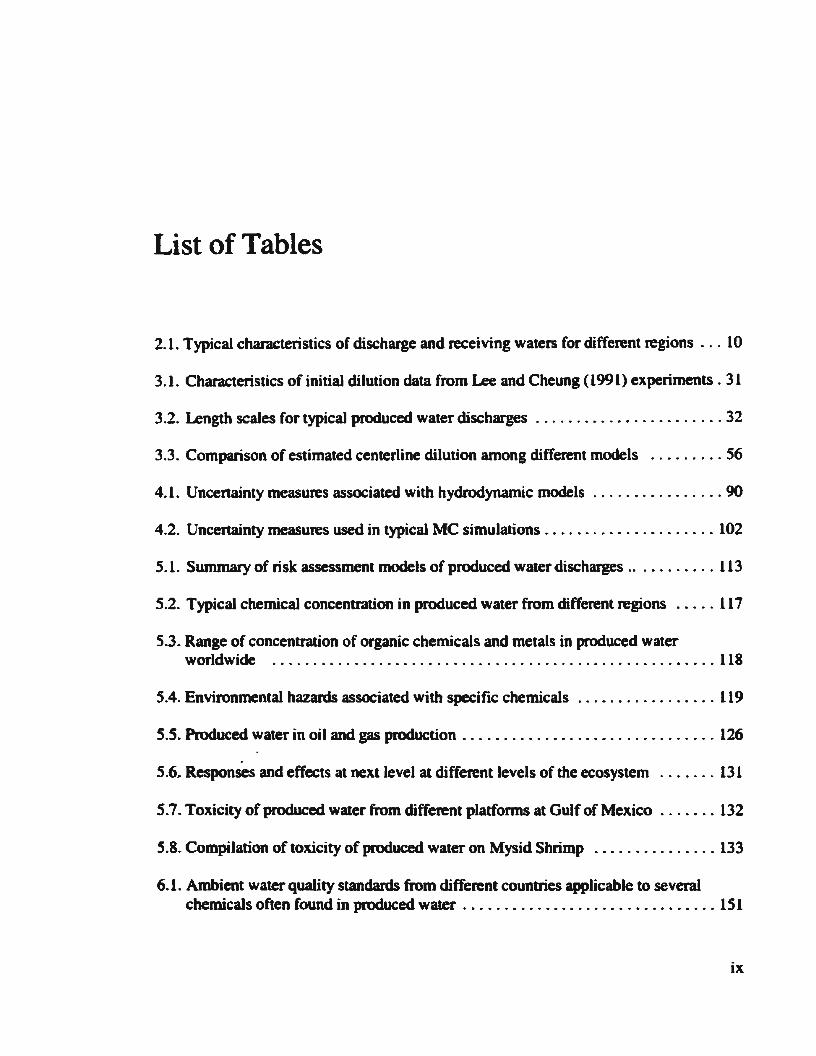
List of Tables
2.1. Typical characteristics of discharge and receiving waters for different regions ... 10
3.1. Characteristics of initial dilution data from Lee and Cheung (1991) experiments . 31
3.2. Length scales for typical produced water discharges ....................... 32
3.3. Comparison of estimated centerline dilution among different models ......... 56
4.1. Uncertainty measures associated with hydrodynamic models ................ 90
4.2. Uncertainty measures used in typical MC simulations ..................... 102
5.1. Summary of risk assessment models of produced water discharges ........... 113
5.2. Typical chemical concentration in produced water from different regions ..... 117
5.3. Range of concentration of organic chemicals and metals in produced water worldwide . . . . . . . . . . . . . . . . . . . . . . . . . . . . . . . . . . . . . . . . . . . . . . . . . . . . . . 118
5.4. Environmental hazards associated with specific chemicals ................. 119
5.5. Produced water in oil and gas production ............................... 126
5.6. Responses and effects at next level at different levels of the ecosystem ....... 131
5.7. Toxicity of produced water from different platforms at Gulf of Mexico ....... 132
5.8. Compilation of toxicity of produced water on Mysid Shrimp ............... 133
6.1. Ambient water quality standards from different countries applicable to several chemicals often found in produced water ............................... 151
ix

6.2. Typical module weights in the FPSO ................................. 157
6.3. Species caught commercially in Grand Banks and landed at Newfoundland pons between 1992-1994 ........................................... 162
6.4. Preliminary discharge scenarios for the case study ................... ... .. 168
6.5. Initial dilution associated with the preliminary discharge scenarios ....... . .... 172
6.6. Typical results from whole effluent toxicity tests ......................... 189
6. 7. Feeding relationships among species in terms of stomach contents of common fish species . . . . . . . . . . . . . . . . . . . . . . . . . . . . . . . . . . . . . . . . . . . . . . . 191
6.8. A summary of available data on ecological effects of Cd on different species .. 193
X

List of Figures
1.1. Schematic diagram of the research . . . . . . . . . . . . . . . . . . . . . . . . . . . . . . . . . . . . . 6
2.1. Schematic depiction of buoyant jet and plume following a produced water discharge from offshore oil fields (not to scale) ...... . ..... 12
2.2. Sketch definition for typical initial dilution modeling ..................... 13
2.3. Curve fitting of asymptotic solutions and laboratory data ................... 21
2.4. Discontinuity of asymptotic solutions proposed by Lee and Cheung ( 1991) ..... 22
2.5. Comparison between initial dilution models and laboratory data ............ 24
2.6. Residuals at different region for the Huang et al. (1998) model .............. 25
3.1. Plot SQ/ut versus lllb for 107 sets of data from Lee an Cheung (1991) ........ 34
3.2. Deterministic and probabilistic fit of the models to the data ................. 44
3.3. Comparison between the Huang et al. (1998) model and equation 3.19 ........ 45
3.4. Residuals of the Huang et al. (1998) model ............................. 46
3.5. Residuals of equation 3.19 .......................................... 46
3.6. Comparison between calculated dilution (Huang et al. 1998) and the data ...... 48
3.7. Comparison between calculated dilution (equation 3.19) and the data ......... 49
3.8. Comparison between calculated dilution {Ue and Cheung 1991) and the data ... 49
3.9. Comparison of percentage error of calculated dilution ..................... 50
xi

3.10.1nfluential points producing high residuals in the models .................. 51
3.11. Probability plot of residuals for the Huang et al. ( 1998) model with outliers ... 52
3 .12. Probability plot of residuals for the proposed model with outliers ............ 52
3.13. Probability plot of residuals for the Huang et al. (1998) model without outliers . 53
3.14. Probability plot of residuals for the proposed model without outliers ......... 53
3.15. Flow chart of the procedure of evaluating probability of failure associated with uncertainty in the model . . . . . . . . . . . . . . . . . . . . . . . . . . . . . . . . . . . . . . . . 57
4.1. Various discharge characteristics ...................................... 64
4.2. Typical intermediate region of discharges ............................... 69
4.3. A typical sketch definition of buoyant spreading ......................... 76
4.4. Coordinate definition for locating plume movement ....................... 81
4.5. Typical grid points showing nodes for the simulation ...................... 82
4.6. Concentration distribution (% ), a plan-view of the produced water plume ...... 84
4. 7. CORMIX output, a plan-view of the produced water plume ................ 85
4.8. Lognormal distribution of daily-averaged current speeds ................... 92
4.9. Beta distribution of daily-averaged direction of currents ................... 93
4.10. A typical comparison of random sampling and LHS-based MC simulations ... 103
4.11. Distribution of produced water concentration at 100-m downstream ......... 104
4.12. Exceedance probability for typical threshold concentrations ............... 104
4.13. Distribution of the mean concentrations ............................... 105
4.14. Distribution of the 95%-tile concentrations ............................ 106
4.15. Distribution of the maximum concentrations(%) ....................... 106
5 .1. General framework of ecological risk assessment . . . . . . . . . . . . . . . . . . . . . . . . 115
xii
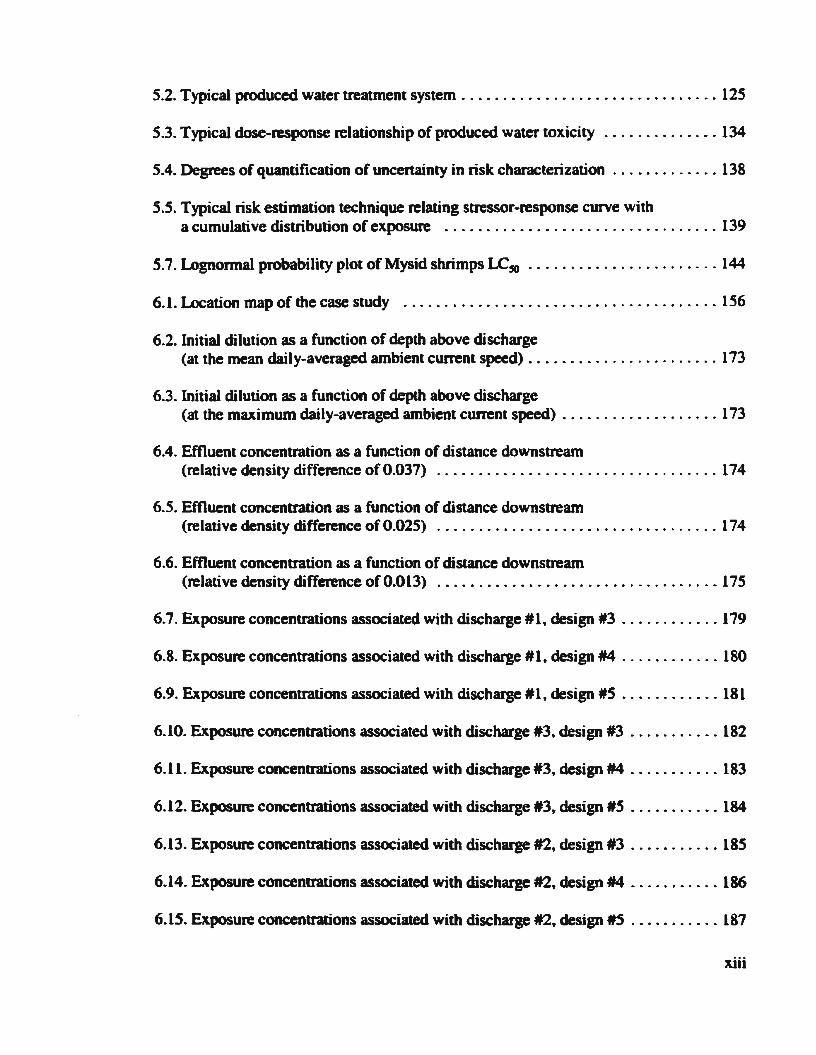
5.2. Typical produced water treatment system ............................... 125
5.3. Typical dose-response relationship of produced water toxicity .............. 134
5.4. Degrees of quantification of uncertainty in risk characterization ............. 138
5.5. Typical risk estimation technique relating stressor-response curve with a cumulative distribution of exposure ................................. 139
5.7. Lognormal probability plot ofMysid shrimps LC50 •••••••••••••••• • •••••• 144
6.1. Location map of the case study . . . . . . . . . . . . . . . . . . . . . . . . . . . . . . . . . . . . . . 156
6.2. Initial dilution as a function of depth above discharge (at the mean daily-averaged ambient current speed) ....................... 173
6.3. Initial dilution as a function of depth above discharge (at the maximum daily-averaged ambient current speed) ................... 173
6.4. Effluent concentration as a function of distance downstream (relative density difference of 0.037) .................................. 174
6.5. Effluent concentration as a function of distance downstream (relative density difference of 0.025) .................................. 174
6.6. Effluent concentration as a function of distance downstream (relative density difference of 0.013) ........................... . ...... 175
6.7. Exposure concentrations associated with discharge #1, design #3 ............ 179
6.8. Exposure concentrations associated with discharge #1, design #4 ............ 180
6.9. Exposure concentrations associated with discharge #1, design #5 ............ 181
6.10. Exposure concentrations associated with discharge #3, design #3 ........... 182
6.11. Exposure concentrations associated with discharge #3, design #4 ........... 183
6.12. Exposure concentrations associated with discharge #3, design #5 ........... 184
6.13. Exposure concentrations associated with discharge #2, design #3 . . . . . . . . . . . 185
6.14. Exposure concentrations associated with discharge #2, design #4 ........... 186
6.15. Exposure concentrations associated with discharge #2, design .S ........... 187
xiii

6.16. Plotting position for the toxicity data summarized in Table 6.8 ............. 193
6.17. Whole effluent chronic hazard quotients, design #3 (fish survival risks) ...... 197
6.18. Whole effluent chronic hazard quotients, design #3 (shrimp survival risks) ... 198
6.19. Whole effluent chronic hazard quotients, design #4 (fish survival risks) ...... 199
6.20. Whole effluent chronic hazard quotients, design #4 (shrimp survival risks) ... 200
6.21. Whole effluent chronic hazard quotients, design #5 (fish survival risks) ...... 201
6.22. Whole effluent chronic hazard quotients, design #5 (shrimp survival risks) ... 202
6.23. Exceedance probability of the whole effluent chronic benchmark (fish survival risks, design #3) ....................................... 203
6.24. Exceedance probability of the whole effluent chronic benchmark (Shrimp survival risks, design #3) . . .................................. 203
6.25. Exceedance probability of the whole effluent chronic benchmark (fish survival risks, design #4) ....................................... 204
6.26. Exceedance probability of the whole effluent chronic benchmark (Shrimp survival risks, design #4) .................................... 204
6.27. Exceedance probability of the whole effluent chronic benchmark (fish survival risks, design #5) ....................................... 205
6.28. Exceedance probability of the whole effluent chronic benchmark (Shrimp survival risks, design #5) ....•............................... 205
6.29. Chemical specific, 226Ra hazard quotients, design #3 (risks on fish) ......... 207
6.30. Chemical specific, 226Ra hazard quotients, design #4 (risks on fish) ......... 208
6.31. Chemical specific, 226Ra hazard quotients, design #5 (risks on fish) .... . .... 209
6.32. Exceedance probability of the 22~a benchmark, design #3 ................ 210
6.33. Exceedance probability of the 226Ra benchmark, design #4 ................ 210
6.34. Exceedance probability of the ~a benchmark, design #3 ................ 211
6.35. Cadmium protection level (the 95% aquatic species toxicity thresholds)
xiv
and associated probability ......................................... 213
6.36. Exceedance probability of the Cd protection level. design #3 .............. 214
6.37. Exceedance probability of the Cd protection level, design #4 .............. 214
6.38. Exceedance probability of the Cd protection level, design #5 .............. 215
6.39. Exceedance probability of the 90 Cd protection level {design #3) .......... 220
6.40. Exceedance probability of the 90.Cd protection level (design #5) .......... 220
XV

List of Symbols and Abbreviations
List of symbols:
a :coefficient of the Huang et al. (1998) initial dilution model.
a1, a2 :coefficient of the functional relationship of hydrofynacmic characteristics at
various region. i.e. BDNF. transition, and BDFF.
A( z) : area of the Standard Nonnal Distribution from 0 to z along the abscissa.
b : coefficient of the Huang et al. ( 1998) initial dilution model.
B : discharge specific buoyancy flux (m4/sec3).
c : coefficient of the Huang et al. (1998) initial dilution model.
C" : bulk pollutant concentration at the downstream end of the control volume.
C1 :coefficient of the Lee and Cheung (1991) initial dilution model.
C2 :coefficient of the Lee and Cheung (1991) initial dilution model.
C1 : coefficient of the equation of the horizontal boil location.
C., : coefficient of the equation of the horizontal boil location. it is a function of the
ratio of buoyancy and momentum length scales.
C5 : coefficient of the equation of the horizontal boil location.
C01 : coefficient of the equation of distance from the boil center to the downstream
end of the control volume.
xvi

C 02 : coefficient of the equation of distance from the boil center to the downstream
end of the control volume.
Cs1 : coefficient of the equation of the bulk dilution at the downstream end of the
control volume.
C 52 : coefficient of the equation of the bulk dilution at the downstream end of the
control volume.
C(x,y) :pollutant concentration at a point (x,y).
d : diameter of the outfall port (m).
d2 :coefficient of the Huang et al. (1998) initial dilution model.
e :coefficient of the proposed initial dilution model.
£ 1 : forced entraintment.
£ 1 : shear entraintment.
er/(w) : the enor function of w.
EC50 :pollutant concentration resulting in observed effect in 50% test animals.
f :coefficient of the proposed initial dilution model.
f : count of the failure cases in Monte Carlo simulations.
Fo :jet densimetric Froude number (dimensionless).
g : gravitational acceleration (mlsec2).
g' : reduced gravitational acceleration (mlsec2).
h : coefficient of the proposed initial dilution model.
ho : plume thickness (m).
h(x) : plume thickness (m) as a function of distance x.
H : depth of the ambient water (m).
xvii

Io.1 :regional variables (hydrodynamic characteristics) at the transitional regime
define as Hll, > 0. L
110 :regional variables (hydrodynamic characteristics) at the transitional regime
define as H/16 < 10.
~r : regional variables (hydrodynamic characteristics) at the transitional regime
define at 0.1 ~ HA, ~ 10.
1, : length scale (m) as a measure of the vertical distance at which the velocity
induced by the buoyancy has decayed to the value of the ambient velocity.
1,. : length scale (m) as a measure of the interaction of a momentum-dominated jet
with a cross-flow.
1M : length scale (m) as a measure of the distance at which the buoyancy becomes
more important that the jet momentum.
IQ : length scale (m) as a measure determining whether the jet geometry has a direct
influence on the flow characteristic.
LC 10 :pollutant concentration resulting in observed lethal effect in 10% test animals.
~ : pollutant concentration resulting in observed lethal effect in 25% test animals.
LC50 : pollutant concentration resulting in observed lethal effect in 50% test animals.
LC75 : pollutant concentration resulting in observed lethal effect in 75% test animals.
L, : plume width at the downstream end of the control volume (m).
LJ :upstream intrusion length (m).
Ux) : plume width (x) as a function of distance x.
M : discharge momentum flux (m4/s1).
n : number of species for which toxicity data is available for a particular chemical.
xviii

N : number of sample (data points).
ns : number of simulations performed in Monte Carlo simulations.
p-value: the smallest level of significant at which hypothesis would be statistically
rejected.
Q :outfall discharge (flow) rate (m3/sec)
r : count of the reliable cases in Monte Carlo simulation.
R 2 : coefficient of detennination.
R1 : flux Richardson number.
S :initial (centerline) dilution.
sa : bulk dilution at the downstream end of the control volume (dimensionless).
TU:a :acute toxicity unit.
TUc : chronic toxicity unit.
u : ambient current speeds (m/s).
u. : shear velocity (mls).
ui : initial jet velocity (m/s).
w :coefficient of the proposed initial dilution model.
x : distance along the plume centerline staning from the center of the downstream
end of the control volume (m).
xb : horizontal distance of the boil location from the port (m).
x0 : distance from the boil center to the downstream end of the control volume (m).
X : global coordinate system in the horizontal direction.
Y : global coordinate system in the vertical direction.
z : depth above discharge (m).
xix

a : entraintment coefficient.
p : constant in the equation of buoyant spreading.
E : error tenn in the proposed initial dilution model.
~ : value of the jth parameter minus its starting value in the iteration process of
the nonlinear regression.
Pu : density of ambient seawater {kglm3).
Po : density of the effluent (kglm3).
K : von Kannan constant.
8 : angle between the rising buoyant jet axis and the water surface (radian).
t/J : direction of the current with respect to the X -coordinate system (radian).
~i : derivative of the nonlinear function with respect to the jth parameter, used in
the nonlinear regression.
List of abbreviations:
AAN : Artificial neurol network.
ANZECC : Australia and New Zealand Environment and Conservation Council.
ARMCANZ : Agriculture and Resource Management Council of Australia and
BC
BDFF
BDNF
BTEX
CCME
New Zealand.
: Benchmark concentration.
: Buoyancy-dominated far field.
: Buoyancy..<fominated near field.
:Benzene, Toluene, Ethylene and Xylene.
: Canadian Council of Ministers of the Environment.
XX

CCB
CCC
CDF
CHARM
CORMIX
CMC
DFO
DREAM
EC
ERA
FPSO
FOSM
GBS
GM
HHC
HQ
LDEQ
LHS
MC
MSE
NOEC
ooc
PAH
: Critical body burden.
:Criterion continuous concentration.
:Cumulative distribution function.
: Chemical Hazard Assessment and Risk Management.
: Cornell Mixing Zone Expert System.
: Continuous maximum concentration.
: Department Fisheries and Ocean.
: Dose related Risk and Effects Assessment Models.
: Exposure concentration.
: Ecological risk assessment.
: Floating Production, Storage and Offloading.
: First Order Second Moment.
:Gravity-based structures.
: Geometric mean.
:Human health criterion.
: Hazard quotient.
: Louisiana Depanment of Environmental Quality.
: Latin hypercube sampling.
: Monte Carlo, it is used to refer Monte Carlo simulations.
:Mean square error.
: No observed effect concentration.
: Offshore Operators Committee.
: Polycyclic aromatic hydrocarbon.

PEC
PNEC
RSB
RSM
TU
U.S. EPA
VIF
: Predicted environmental concentration.
: Probability density function.
: Predicted no effect concentration.
: Roberts, Snyder and Baumgartner.
: Response surface methodology.
: Toxicity unit.
:United States Environmental Protection Agency.
:Variance inflation factor.
xxii

Chapter 1
Introduction
1.1. Background to Study
Associated with oil drilling and production are various types of wastes. These include
drilling fluids, drill cuttings, produced water, produced sand, deck drainage. sewage,
domestic wastes, and treatment chemicals. The major waste streams in terms of volumes
and amount of pollutants are drilling fluids and drill cuttings from drilling operations and
produced water from oil production operations. The term produced water refers to the water
(brine) brought up from the hydrocarbon-bearing strata during the extraction of oil and gas,
and can include formation water, injected water, and any chemical added downhole or
during the oil/water separation process (U.S. EPA 1993).
The quantity of produced water from an oil field varies from case to case depending upon
the characteristics of the oil reservoir and the age of the field. Typical examples of
produced water discharge rates from offshore fields are on the order of 4,000 m3/day in the
Guif of Mexico, USA, to 123,000 m1/day in the Java Sea. Indonesia (Brandsma and Smith
1

1996. Smith et al. 1996, Somerville et al. 1987). Considering the rate of oil or gas
production at a given platform. the flow rate of produced water is usually very substantial.
From the EPA's 30-facility study (U.S. EPA 1993), it is reported that produced water flow
rates range from 2 to 150,000 barrels per day. with associated production rates of 40 to
24,000 barrels per day and 0.1 to 150 million cubic feet per day for oiVcondensate and gas.
respectively. Generally, produced water can account for between 2 to 98% of the extracted
fluids from the reservoir (Stephenson 1992, Wiedeman 1996). As a result, cost-effective
and environmentally acceptable management and disposal of produced water is critical in
the petroleum industries.
The chemical composition of produced waters is site specific, and includes a variety of
inorganic, organic, and radioactive chemicals (Roe et al. 1996, Stephenson 1992). For
offshore and coastal oil industries, produced water is often discharged into the ocean.
following a treatment at the platform. The type and degree of the treatment depends on the
end use of the water or disposal method. Although a treatment is provided before discharge,
the produced water effluent commonly still contains toxic chemicals, making it an
environmental concern.
Typical produced water from North Sea platforms has been associated with ecological
impacts, which are reported in terms of effect concentration with 50% reduction in growth
(ECso, based on two-day exposure) of 45 to 535 mVl for algae (Brendehaug et al. 1992).
Lethal concentration with SO% mortality based on one-day exposure (LC50) was 100 mill
for the copepod Calanus jinmarchicus (Sommerville et al. 1987). For fish, the lowest value
2
registered of LCso is for the guppy~ Poecilia retivulata, at a value of 7.5-423 mill (Jacobs
and Marquenie 1991). Based on the evidence of toxicity~ environmental risk management is
becoming increasingly important in offshore oil production (Ofjord et al. 1996).
When produced water is discharged into the ocean, the process is subject to compliance
with relevant water quality standards. Recently, there has been a trend towards specifying
pollutant limits from ecological and epidemiological viewpoints, in which pollutant
concentrations are specified in tenns of ecological and human health risks (ANZECC and
ARMCANZ 1999, U.S. EPA 1999a). This raises the possibility that design of the produced
water outfall could itself be looked at from the point of view of ecological risk due to
exposure to produced water or specific toxic poUutants associated with it.
Ecological risks have been assessed for specit'ic pollutants found in produced waters from
offshore fields (Funsholt 1996, Karman et al. 1996, Neff and Sauer 1996, Ofjord et al.
1996). However, there are drawbacks associated with presently used approaches for
ecological risk assessment of produced water discharges. These are that endpoints of the
assessment are not well defined, and that uncertainty analysis is not carried out objectively.
Furthennore, risk assessments are usually directed at monitoring or remediation purposes,
rather than design. In particular, ecological risk assessment (ERA) has not been
incorporated during the engineering design of produced water outfalls.
The risks associated with the offshore discharge of produced waters depend strongly on the
contaminant distribution in the ambient seawater (Kannan and Reerink 1998, Meinhold et
3
al. 1996a. Smith et al. 1996. Stromgren et al. 1995, Girting 1989, Somerville et al. 1987).
Hydrodynamic modeling plays an important role in assessing contaminant levels for ERA
studies; however, there appears to be no generally accepted model for such a purpose.
Presently available approaches to hydrodynamic modeling have inherent problems. The
first problem is related to the reliability of the initial dilution models. This includes
assumptions taken in developing the models and the numerical accuracy of the models as
discussed in more detail in Chapter Two. Another problem is that presently used
approaches (e.g. Wasbum et al. 1999, Kannan et al. 1996, Reed et al. 1996, Brandsma et al.
1992, Somerville et al. 1987) do not provide uncenainty analysis, and that exposure
concentration at a fixed distance from the platfonn is calculated using a deterministic
approach. Indeed. uncertainty is inherent and inevitable in the mixing processes between
the produced water and the ambient seawater. Therefore, there is a need to develop a
probabilistic hydrodynamic model, which could be integrated into an ERA model, for
ecological risk-based design of produced water outfall.
1.2. Scope and Purpose of the Research
This study has two major components: hydrodynamic modeling and ERA. The previous
section has briefly discussed the problems, which will be critically reviewed in subsequent
chapters. Some limitations need to be established to ensure a realistic scope of the research
project. The general objective of this study was to develop a methodology for an ecological
risk-based design of produced water discharge from an offshore platfonn. This was carried
4

out through integrating a probabilistic hydrodynamic model with an ERA model as shown
schematically in figure 1.1.
As indicated in figure 1.1, the hydrodynamic modeling consists of the development of an
initial dilution model and its integration with a far field model. The study was directed at
the case of buoyant-jet discharge in unstratified moving waters. The deterministic far field
models were adapted from the published models and their development is beyond the scope
of this research. The integrated hydrodynamic model was used in the development of a
methodology for ERA. A framework for ecological-risk based design of produced water
outfall was then developed using the integrated hydrodynamic and ERA model. A case
study was presented to highlight a potential application of the proposed methodology.
Probabilistic and uncenainty analysis was applied throughout the modeling process.
Keeping in perspective the above problem formulation, this research has the following
more specific objectives:
l. developing an initial dilution model;
2. integrating the developed initial dilution model with far field dilution models;
3. developing a methodology for probabilistic hydrodynamic modeling;
4. identifying methodologies for ecological risk assessment of produced water
discharge;
5. developing a framework for ecological risk-based design of produced water outfalls;
6. Applying the framework of ecological-risk based design for a case study of outfall
design for an offshore oil platfonn.
5

Length scele end dimensional enalysis
INmAL DILUTION MODELING
Dell collection for initlel dilution of ttuoyent·jet discharges
Slelislicel evalualion of experimental data
PROIAIILISnC HYDRODYNAMIC MODELING
Plume location, control volume and fer tield dilution models
The developed initial dilution model
Unctflainty information for the models and input veriables
lntegreted hydrodynamic modeling
Development of a methodology far 1 probabilistic enalysis
ECOLOGICAL RISK ASSESSMENT AND ECOLOGICAL RISK· lASED DESIGN OF PRODUCED WATER OUTFALL
ldentlflcetion of methodologies for ecologicet risk eueaament of produced water discharge
Selection of a ceae study lnd design scenlriOS
Development of 1 framework tor ecologicel risk·besed design
AppticetiOn exemplt: characteriZation of ecologicll risk for tile apecllild scenerios
Figure 1.1. Schematic diagram of the resean:h
6

l~.Oudmeof~eTbnu
The thesis consists of eight chapters. Background, objectives and outline of the thesis have
been presented in this chapter. Chapter Two presents a critical review dealing with
problems of presently available initial dilution models and discusses potential initial
dilution modeling approaches, which may be useful to overcome the drawbacks discussed.
Development and evaluation of an initial dilution model are presented in Chapter Three, in
which a new approach to initial dilution modeling is proposed. A unique initial dilution
model is presented in a detenninistic and probabilistic form. An application example of the
proposed model is also provided. Chapter Four provides reviews of approaches to
integrating near and far field models in hydrodynamic modeling of produced water
discharges. A probabilistic hydrodynamic modeling approach is formulated in this chapter.
Chapter Five reviews available approaches to ecological risk assessment (ERA) and
identifies methodologies of ERA in the context of produced water discharges.
Chapter Six provides a framework of ecological risk-based design for produced water
outfall. A case study using data on potential discharge from the Terra Nova Floating,
Production, Storage and Offioading (FPSO) system, located at the Grand Banks,
Newfoundland, Canada (Petro-Canada 1996) is also given in this chapter. Different design
scenarios are evaluated on the basis of ecological risks. This makes it possible to classify
alternative designs (e.g. different geometries and/or different locations of outfalls)
according to the ecological risks, which might arise from the discharge scenario, and to
determine the degree to which one design is more appropriate than another. Conclusions
7

and recommendations are presented in Chapter Seven, and the statement of originality of
the thesis is given in Chapter Eight.
8

Chapter2
Initial Dllution in Hydrodynamic Modeling: Problems of Presently Available Models and Potential Modeling Approaches
2.1. Introduction
Once produced water is discharged into the ocean, it mixes with the ambient seawater. The
flow pattern of the discharge may be categorized as a buoyant jet flow as it is often found
that the discharge has both initial momentum and a density difference between the effluent
and the ambient seawater. Table 2.1 provides a summary of produced water discharges and
receiving water conditions from different regions. A typical discharge from a Nonh Sea
platform has a discharge rate of 10,000 m3 per hour and a density difference of 13 kglm3
less than ambient seawater (Somerville et at. 1987). Smith et at. (1996) noted that typical
characteristics of a discharge result in a buoyant plume that comes to the surface within 10
meters of the open-ended outfall.
Hydrodynamic characteristics of the discharge of produced water play an important role in
governing the fate of the effluent. Considerable attention has been given to modeling
9

hydrodynamic mixing between the effluent and the ambient seawater for the assessment of
the environmental impact (Smith et al. 1996, Brandsma and Smith 1996, Stromgren et al.
1995, Somerville et al. 1987) and ocean environmental risks (Kannan and Reerink 1998,
Meinhold et al. 1996). In addition to plume ttajectory and turbulent diffusion, initial
dilution is one of the most important measures in such a hydrodynamic modeling
(Washburn et al. 1999, Smith et al. 1996, Stromgren et al. 1995, Somerville et al. 1987).
This chapter outlines the definition of initial dilution and its use in design of effluent
discharges. Critical reviews on presently available initial dilution models are presented. It
also discusses potential modeling approaches in dealing with drawbacks of the models.
Table 2.1 Typical characteristics of discharge and receiving waters for different regions (data from Brandsma and Smith 1996. Smith et al. 1996, Somerville et al. 1987)
Region Parameters
Bass Strait Gulf of Mexico Java Sea NonhSea
Discharge Rate (m3/day) 14,000 3977.8 26.235- 10,000 123.225
EflnuentTe~~(°C) 90 29 62-90 30
Eflnuent Density (kglm3) 988 1088 - 1014
Ambient Density• (kg/m3) 1026 1017 - 1027
Density Gradient (kg/m•) 0 0.15 - 0
Port Diameter (m} or Holes of 0.2 0.2 0.76
Discharge configuration 2"x4''
Depth above Discharge (m) 12 0.3 3-15 s Port Orientation Downwards Downwards Radial Horizontal
Sea Water Depth (m) 72 27.4 21.3-30.5 150
Sea Water Speed (mls) 0.3 0.03-0.25 - 0.3
*ambient density in the area closed to the discharge poinL
10

2.2. Initial DUution in Hydrodynamic Mode6ng and Design
In modeling, hydrodynamics of produced water effluent from an ocean outfall can be
conceptualized as a mixing process occurring in two separate regions. The first region is
referred to as the "near field., in which the initial jet characteristics of momentum flux.
buoyancy flux. and outfall geometry influence the jet trajectory and mixing. For this region,
designers of the outfall may expect different characteristics of the initial mixing, such as the
degree of dilution, through appropriate manipulation of design variables. The second region
is referred to as the •'far field., where the effluent plume travels farther away from the
source. and the source characteristics become less important. The trajectory and dilution in
the far field are mainly controlled by characteristics of ambient seawater, such as the
strength and direction of seawater currents, through buoyant spreading motions and passive
diffusion (Doneker and Jirka, 1990). A typical schematic depiction of the near and far fields
is shown in Figure 2.1.
In hydrodynamic modeling, initial dilution has been widely used as a measure of the
mixing in the near field By definition, initial dilution is the dimensionless ratio of pollutant
concentration in the wastewater effluent prior to discharge to the concentration at an
equilibrium level: or the free surface, or seabed. Initial dilution can also be expressed in
tenns of centerline dilution, which is dilution at the centerline of the jet above, or below,
the discharge port. Initial dilution occurs because of the entrainment of the surrounding
fluid during the rise or sink of the effluent from the outfall ports. This rising or sinking
motion occurs because of buoyancy resulting from the difference between the densities of
11

wastewater and seawater. Figure 2.2 shows a typical depiction of a rising buoyant jet in a
cunent for typical initial dilution modeling.
Figure 2.1. Schematic: depiction of buoyant jet and plume following a produced water discharge from offshore oil fields (not to scale)
The use of initial dilution for the evaluation of discharge scenarios has been a traditional
practice in the management of various wastewaters. including the release of sewage
discharges. cooling water from a power plant. and produced water from oil production
platfonns. The discharge facility is usually designed in such a way that the effluent mixes
effectively with ambient seawater. The design is not simply to dilute the effluent but. more
12

imponantly. to permit natural processes in the ocean to stabilize the waste with minimal
environmental damage. In such a design. initial dilution is used as one important measure to
investigate the degree of the mixing between the wastewater effluent and ambient seawater.
Proper design ensures that the discharge results in sufficiently high initial dilution with
minimal thickness of the effluent slick. High initial dilution is also required to maintain
acceptably low ecological risks or to comply with relevant water quality standards within a
designated mixing zone.
Figure 2.2. Sketch definition for typical initial dilution modeling
13
2.3. Previous Work on Initial Dilution ModeHng
Many studies have been performed in the past for modeling initial dilution. For a stagnant
ambient water condition. Cederwall (1968) provides a good. simple, empirical initial
dilution model. This model is commonly accepted because its estimated dilution values
generally agree with other theoretically and experimentally derived results (Sharp 1 989a.
Wood et al. 1993). In moving waters, however. there appears to be no universally accepted
model for initial dilution calculations (Sharp and Moore 1989, Sharp and Moore 1987, Lee
and Neville-Jones 1987a).
Mathematical modeling approaches based on the fundamental equations of motion have
been employed for buoyant jets of drilling mud and produced water discharges (Brandsma
et al. 1992. Brandsma et al. 1980, Reed et al. 1996. Skatun 1996). In developing the initial
descent model, for example. the Offshore Operators Committee (OOC) model (Brandsma
et al. 1992; Brandsma et al. 1980) was based on the equations of conservation of mass.
momentum. buoyancy and constituent flux, and further based on the assumption of
independent clouds of the Lagrangian advection-dispersion scheme. The mathematical
models for initial dilution are theoretically sound. but suffer from a lack of well
documented, detailed data for validation (Sharp and Moore 1987). When applying
mathematical models. Andrade and Loder ( 1997) noted that the application should not be
viewed as reliable unless they have been properly validated.
14

Andrade and Loder (1997) compared the perfonnance of mathematical models for initial
dilution calculations. They found that the OOC model provides similar qualitative features
of the plume evolution and, in some cases, close agreement in values of the plume radius
and dilution with those of the United State Environmental Protection Agency (U.S. EPA)
models (Muellenhoff et al. 1985). The OOC model was originally developed for discharge
evaluation of drilling wastes; and the U.S. EPA models are commonly employed for the
analysis of sewage discharges. However. Sharp and Moore (1989) found that the same U.S.
EPA mathematical models typically overestimated dilution by a factor of about 2 to 4.
An alternative approach to the modeling of a buoyant jet is to use empirical equations
derived from experimental data. This approach has been applied for simulating initial
dilution of produced water in the Santa Barbara Channel near Carpinteria, CA eN ashburn
et al. 1999) using the RSB (Robens. Snyder and Baumganner's) model. which is based on
dimensional analysis and on laboratory experime11t~ dP.scribed by Robens et al. ( 1989a-c ).
Empirical equations for initial dilution have also been employed for produced water
discharge from the Krisna platfonn in the Java Sea, Indonesia (Smith et al. 1996). In this
case, the Cornell Mixing Zone Expert System (CORMIX) model (Jirka et al. 1996) was
calibrated and used for initial dilution calculations. CORMIX is computer software that
compiles flow classifications and mixing behaviors of effluent discharges. For a given case
of flow classification, mixing behavior is based on published empirical equations or
experiments.
15

Applying empirical equations for dilution analysis does have the advantage of being based
on physical data (Sharp and Moore 1987), so there is an increased confidence in the
reliability of the modeling. In deriving empirical equations for initial dilution, an
asymptotic approach has been widely used. The approach derives equations with the aid of
dimensional analysis and data from laboratory or field experiments (Wright 1977a, Fisher
et al. 1979, Lee and Neville-Jones 1987~ 1987b, Robert et al. 1989a, 1989b, 1989c, Lee
and Cheung 1991, Wood 1993, and Proni et al. 1994).
Using asymptotic approaches, initial dilution of a round turbulent buoyant jet discharge in
unstratified moving waters can be physically represented by the relevant parameters
(Wright 1977a, Lee and Neville-Jones 1987a, Lee and Cheung 1991):
S =f(Q. M. B, u, Z) (2.1)
in which S is the initial dilution at depth above discharge z: u is the ambient current speed;
and Q is the outfall discharge rate. M is the discharge momentum flux, defined as:
where ui is the velocity of jet discharge. B is the buoyancy flux, defined as:
B =Q g P. -p., P.
(2.2)
(2.3)
16

where g is the gravitational acceleration; and Pa and Po are densities of the ambient
seawater and effluent, respectively. Since all these parameters have units of lengths and
time only, Buckingham's 1t-theorem indicates that the phenomenon can be defined by only
four dimensionless groups.
Following Wright (1977a) and Lee and Cheung (1991), the jet·ambient parameters can be
combined into length scales, each of which characterizes a panicular aspect of the general
problem. The two length scales that characterize the jet discharge are IM and IQ. which are
defined as:
(2.4)
(2.5)
where d is the diameter of the port. The length scale IM is a measure of the distance at which
the buoyancy becomes more important than the jet momentum; the length scale IQ is a
measure determining whether the jet geometry will have a direct influence on the flow
characteristics.
In the presence of an ambient velocity, two more length scales can be formed, i.e. I"' and lb.
which are defined as:
M 112
l =. " (2.6)
17

B lb =-J
u (2.7)
The length scale lm relates to the interaction of a momentum-dominated jet with a cross-
flow; and the length scale lb represents the vertical distance at which the velocity induced
by the buoyancy (proportional to 8 113 1'i8 ) has decayed to the ambient v.:Jocity value u.
If the functional relationship in equation (2.1) is expressed in non-dimensional parameters
fonned from the various length scales, one possible result is {Wright 1977a):
( IQ l. z)
S=f -, ,-1 'l , • It
(2.8)
In dealing with this problem, a simplified solution using an asymptotic approach is usually
adopted (Lee and Neville-Jones 1987a, Lee and Neville-Jones 1987b, Wright 1977a)
because of the number of independent parameters that must be considered. In this approach,
the number of independent factors affecting the system is reduced through physical
reasoning. For instance, by considering the effects of the jet momentum and the buoyancy
separately, the number of independent parameters is reduced. For buoyancy dominated
discharges, 1,/lb << l, and for negligible volume flux, 1(/lb << 1, the relationship in
equation (2.8) becomes (Lee and Cheung 1991):
(2.9)
18

The relation developed using the asymptotic solutions is interpreted by examining the
relative magnitude of the various length scales, primarily 1, and lb. and by assuming that the
analysis is to be applied for distances somewhat greater than Ia from the source.
Large numbers of initial dilution models have been developed using this approach for
different cases (e.g. Wright 1977a. Fischer et al. 1979, Wood et al. 1993). For buoyancy
dominated discharges, e.g. freshwater discharges into the ocean, the following relationships
are common! y used (Lee and Cheung 1991 ):
( )
S/3
SQ=C ..£ u/2 t I
b b
forBDNF (2.10)
SQ =C (..£)2 u/2 2 I
b b
forBDFF (2.11)
The tenns BDNF and BDFF refer to the condition of the discharges. i.e. buoyancy-
dominated near field (BDNF) for (zllb <<1) and buoyancy-dominated far field (BDFF) for
(zllb >>1). The coefficients C1 and C2, were determined from experimental data, and are 0.1
and 0.51 for the BDNF and BDFF, respectively (Lee and Cheung 1991).
The reliability of using asymptotic solution-based initial dilution models has been
addressed from several aspects. Analytically, Sharp (1989b) noted that reananging these
equations reveal that the ambient current speed is absent in the BDNF zone, and the
effluent buoyancy will have no effect in the BDFF zone. The model is therefore
conceptually questionable. Lee and Neville-Jones (1989) noted that for moderately small
19

values of zllb of about 0.1, the dilution can exceed the dilution in still water by a factor of 2
or 3, and that this phenomena may be related to a marked change in flow structure (iet
bifurcation). However, it was shown in the field observations of the Hollywood outfall that
a low value of z/16 of about 0.04 to 0.1 was associated with ambient seawater currents of
about 8.5 to 10 crnls (data from Proni et al. 1994). This suggests that effects of the ambient
seawater current are not negligible even in cases with moderately small values of zllb. and
thus should not be missing in the model formulation (BDNF).
Numerically, the asymptotic solutions (equations 2.10 and 2.11) can also be of concern.
Figure 2.3. presents a curve fitting of equations 2.10 and 2.11 with the data from Lee and
Cheung ( 1991 ). Traditionally, the dilution data were plotted in the form of SQ I ul; versus
lll, (Lee and Neville-Jones 1987a, Lee and Cheung 1991, Wood 1993, Proni et al. 1994).
Huang et al. (1998) suggest that the data may be plotted in the form of SQ/uz~ versus z/16
so that the transition between BDNF and BDFF is clearly identified. From Figure 2.3 it is
shown that the transition region is evident at lAb about 0.05 to 0.5.
It can be seen in Figure 2.3 that in the BDNF region, in general, equation 2.10
underestimates dilution. There may be significant bias as the figure is presented in log-log
form. It is also evident that using either the BDNF or BDFF equation may result in a
substantial enor when it is applied in the transitional region. Facing this problem, Lee and
Cheung ( 1991) estimated a value of initial dilution for the transitional region using the
BDNF equation with a modified coefficient of C1 = 0.21.
20

The use of the BDNF equation with the modified coefficient seems to be practical. but it is
unrealistic when considering the nature of the data in the transition region. Consider data in
the transition region. unlike the slope of the data in the BDNF region. the slope in the
transition region is not negative as the data suggest. If continuous solution from the BDNF
through the transition to the BDFF is expected. then the slope in the transition region
should be positive. Not only does the modification (Lee and Cheung 1991) give unrealistic
slope but also discontinuity of solutions between the regions (as shown in Figure 2.4).
-
10~======~======~==~--=-------=-------~ •: I • Data (Lee and Cheung 1991 )
· · · BONF (Lee and Cheung 1991) -BDFF (Lee and Cheung 1991)
.
I
... . : . : . N • • • . • •
a-::1 1 -·················-;·-· ········· .•.•••• ; •••••••••..•.•••••.. ; . . ................ . , ... ............... . .. ... . : : . . : : • ! •• :• :• • • • : • : • va .. •. . a••tos • ••.
···-~. : - al• \~=.-., •a: •: . . • • : • ·I : • I •• : . ·. •• •• • •\li : : : · . ~·"'! • • .. : • . ·· !. • • . ..
0.1 +---------~--------~--------~------~~------~ 0.001 0.01 0.1 1 10 100
Figure 2.3. Curve fitting of asymptotic solutions and laboratory data
Lee and Neville-Jones (1989) noted that the concept of a BDNF and BDFF is strictly valid
only for lllb << 1 and >> 1, respectively. However, in the field, not all cases of ocean
outfall can exactly be classified into one of the regions (BDNF or BDFF). For example,
21

field studies of South Florida outfalls reveal that the outfalls can be characterized as being
in the transitional region, i.e. between BDNF and BDFF (Hazen and Sawyer 1994.
Mukhtasor et al. 1999b, Proni et al. 1994). This raises more evidence of the need of
developing an alternative initial dilution model applicable for such a case.
10~----------------------------~---------:--------~
•. I
BDN~ ~ Tr11n11t1on ~ BDFF ; ! ; 1 1 11 I : : : : I . . . . .
. . ~. ···•·•· ..... -~-................. ·1······· ·;;~··· .... +·· ............ ·-·~·-· ................ 1' . . :• :• . : . : . •· : • · ·-a•·w ···= 1 • • ., • . = :::::zil •• •: I • : • • : • ....... •• I
• • • •• • • • : •eoor • . ~. !
0.1 +---------+---------~------~~--~----~------~~ 0.001 0.01 0.1 1 10 100
Figure 2.4. Discontinuity of asymptotic solutions proposed by Lee and Cheung (1991)
To overcome the above problems, alternative transitional initial dilution models have been
proposed Alternative models were developed using a dimensional analysis combined with
a statistical analysis (Hazen and Sawyer 1994, Proni et al. 1994). The models were based
on data from field studies of South Florida outfalls, specifically two single-port discharges
gfollywood and Broward outfalls) and two diffuser discharges (Miami..Centtal and Miami-
North outfaUs). A probabilistic initial dilution model using the same approach (i.e. a
22

dimensional analysis combined with a statistical analysis) is also available for single pon
discharge based on data from the Hollywood outfall (Mukhtasor et al. 1999b ). However,
these models are limited for the transition region defined by <ilb ranging from 0.04 to 5.
Huang et al. (1998) proposed a centerline initial dilution equation that spans all flow
regimes, from the BDNF, through the transition, to the BDFF. providing continuous
predictions for dilutions. The model was derived based on the continuity equation for the
buoyant jet flow with a hypothesis of additive shear and forced entraintment. Holding this
hypothesis, the Huang et al. (1998) presented the following model:
( )
-1/J SQ z b
u zl =a I; + ( z )-d: 1+c-
lb
(2.12)
where a, b, c, and d2 are model constants, which were detennined by .. trial and error''. In
this approach, the coefficients from Lee and Cheung (1991) were used to determine two of
the four constants in the equation 2.12 (a= 0.10 and b = 0.51). The other two constants
were determined subjectively using the goodness of fit, which was evaluated by eye
(c = 0.10 and d2 = 2). The perfonnance of the model was compared to the asymptotic-based .
solutions and data from Lee and Cheung (1991) as shown in Figure 2.5.
Despite inherent uncertainty because of physical instability as the data suggest, the Huang
et al. (1998) model (equation 2.12) provides unique values of dilution in the transitional
region. As can be seen in Figure 2.5, however, outside the transitional region, solutions
23

given by the Huang et al. (1998) model are practically the same as those given by the Lee
and Cheung (1991) model for BDNF. On the other hand, at zllb > 0.5 the values given by
the Huang et al. (1998) model are somewhat higher that those given by the Lee and Cheung
(1991) model for BDFF. Huang et at's (1998) solutions underestimate dilution at BDNF
and overestimate dilution at BDFF. To investigate the problem more closely, residuals (data
minus estimated value of y-axis) of Figure 2.5 can be evaluated. Based on the data from
Lee and Cheung (1991), a residual plot at different regions of the BDNF, transition and
BDFF, is shown in Figure 2.6. As shown in this figure, the residuals are positive, about
zero, and negative for the BDNF, transition, and BDFF, respectively. This .. structured
bias", together with the use of the unsystematic approach (i.e. trial and error), leads to the
need to develop a new approach to initial dilution modeling for a buoyancy-dominated jet.
10~-------------------------------------------------------------------------~
. . . •: H.ng et •1. (1... BDFF (Lee !lnd Cheung 11[11) . . . .
- • } . . ...... ··:···· .......................................... .. . . . . •
0.1 +. -------~~~------~~~~----~--------~------~ 0.001 0.01 0.1 1 10 100
Figure 2.5. Comparison between initial dilution models and laboratory data (dot point)
24

o.e 0.5 • • 0.4 •
• 0.3
I 0.2 ~ 0.1 &
0.0
.0.1
-0.2
BDNF Tmnsilion 8DFF
Region
Figure 2.6. Residuals at different region for the Huang et al. ( 1998) model
2.4. Potential ModeUng Approaches
Encountering the conceptual and accuracy problems discussed above, alternative
approaches to initial dilution modeling have been proposed. An alternative approach of
modeling was assessed by reanalyzing available experimental data, using methods of the
Artificial Neural Network (ANN) combined with the Response Surface Methodology
(RSM) (Mukhtasor et al. 2000d). ANN is an information processing system that consists of
a number of interconne<:ted computational elements called processing elements or neurons.
By organizing the neurons into different layers and conne<:ting them with proper weights,
networks that are capable of ulearning" can be developed (Malik 1993). In Mukhtasor et al.
(2000d), after training and validation, the ANN perfonnance was then modeled using RSM
which is a colle<:tion of mathematical and statistical techniques for dealing with cases
25

where several independent variables influence a dependent variable, or response, with a
goal of optimizing this response (Montgomery 1976). Detailed description and discussion
of ANN and RSM is not given here, but can be found elsewhere, e.g., Bishop (1994),
Montgomery (1976), Myers and Montgomery (1995), and Smith (1993).
In Mukhtasor et al. (2000d), the ANN was trained using experimental data, and the length
scale ratios (liiQo l/1,.. llib) were used as input parameters of the network. After training, the
network was validated using different sets of data. The RSM was then employed to predict
the performance of the ANN in relating the initial dilution with associated parameters. The
aim of finding a replacement model for the ANN is to come up with a simple initial dilution
model that is easily integrated with other models for further analysis. It was concluded in
that study that the ANN provides better results than asymptotic-based models in terms of
accuracy. However, the ANN-based RSM model did not result in satisfactory results for
replacement of the ANN. The reason for this problem is not clear, but it might be because
the ANN only provided average estimates of initial dilution. The variability of the dilution
data might be then reduced. Therefore, when the outputs of the ANN were used as inputs of
the RSM, models developed by RSM cannot resemble actual initial dilution. These two
methods (RSM and ANN) were then not used further because appropriate laboratory data
specifically suitable for RSM modeling was not available, and because an ANN-based
initial dilution model is not easily integrated with other models such as far field dispersion
models and ecological risk assessment models.
26

Considering the nonlinear nature of the data (see Figures 2.3 to 2.5), it appears that
nonlinear regression modeling combined with length scale analysis may be required to
approach the problem (Mukhtasoret al. 200la). The Huang et al. (1998) model is nonlinear
in nature. but it does not provide a systematic approach to modeling neither objective
measures of the goodness of the fit. Application of the nonlinear regression modeling for
initial dilution is an alternative to the presently available models as discussed in the next
chapter.
2.5. Summary
This chapter discussed the concept of hydrodynamic modeling in tenns of near and far field
models. At the beginning of the chapter, definition of initial dilution and its importance in
the hydrodynamic modeling and outfall design are outlined. Then, presently used modeling
approaches are reviewed and the focus is directed at critical review of conceptual and
numerical problems associated with presently available initial dilution models. Potential
modeling approaches to initial dilution are also discussed in this chapter.
Mathematical models based on the fundamental equations of motion have been proposed in
the past for modeling initial dilution. They are theoretically sound but suffer from a lack of
well documented. detailed data for validation. An alternative approach employs empirical
equations based on physical data; this increases confidence in the reliability of the
modeling. An approach that is widely used to develop empirical initial dilution models is an
asymptotic solution. which derives equations with the aid of dimensional analysis and data
27

from laboratory or field experiments. The asymptotic approach gives a solution that is
limited for two different zones, namely the buoyancy-dominated near field (BDNF) and the
buoyancy-dominated far field (BDFF).
The reliability of using asymptotic solution-based initial dilution models has been
addressed from several aspects. Analytically, it has been conceptually questionable because
rearranging the models reveals that the ambient current speed is absent in the BDNF zone.
and that the effluent buoyancy has no effect in the BDFF zone. Field test data indicated that
even at moderately small values of l/16 the effects of the ambient seawater current can be
quite significant, and should not thus be missing in the model fonnulation (BDNF).
Numerically, based on laboratory data (Lee and Cheung 1991), the asymptotic solution
underestimates dilution in the BDNF region and has no unique solution in the transitional
region. Not only does the manipulation approach to the transitional region adopted in the
previous studies give an unrealistic answer but also discontinuity of solutions between the
regions (BDNF, transition and BDFF). Although it was believed that the concept of a
BDNF and BDFF is strictly valid only for lll6 << 1 and>> 1, respectively, in the field,
some cases of the discharges cannot exactly be classified into one of the regions (BDNF or
BDFF). This raises another question of the applicability of the asymptotic solution for such
cases.
Alternative models have been proposed to overcome the above problems by using a
dimensional analysis combined with a statistical analysis of field data. A probabilistic
initial dilution model using the same approach is also available for single port discharge.
28
However, these models are limited for the transitional region defined by zllb ranging from
0.04 to 5. A model based on the continuity equation with a hypothesis of additive shear and
forced entraintment was proposed as another alternative (Huang et al. 1998), which
provides an equation that spans all flow regimes, from the BDNF, to the transition. to the
BDFF. A systematic approach to modeling and objective measures of the goodness of the
fit are not shown in the Huang et al. (1998) model. This model underestimates dilution in
the BDNF and overestimates dilution in the BDFF. Beside the assumption of stagnant water
adopted for BDNF region, residual analysis shows that this model suffers from the
ustructured bias".
Other potential modeling approaches are also discussed in this chapter. including Artificial
Neural Network (ANN) and Response Surface Methodology (RSM). However, previous
studies show that the ANN provides better results than asymptotic-based models in tenns of
accuracy but the ANN-based RSM models did not result in satisfactory results for the
replacement of the ANN. Considering the nonlinear nature of the data, it appears in this
chapter that nonlinear regression modeling combined with length scale analysis may be
required to approach the problem.
29

Chapter3
Development and Evaluation of Initial Dilution Models
3.1. Introduction
Conceptual and numerical problems associated with presently available initial dilution
models have been discussed in the previous chapter. A nonlinear regression modeling
combined with the additive entrainment hypothesis has been recommended as a potential
alternative approach to modeling initial dilution. This chapter provides a more detailed
description of this modeling. Following discussion on the characteristics of initial dilution.
the approach used in the model development is described. After that, model evaluation and
comparison with presently available models are presented. An application example is
shown at the end of the chapter for deterministic and probabilistic initial dilution modeling.
3.2. Characteristics of Initial Dilution Data
An empirical initial dilution model was developed in this study based on data from Lee and
Cheung (1991). The data was obtained from Lee and Cheung's (1991) series of 48
laboratory experiments (resulting in 107 sets of data) with a buoyancy-dominated vertical
30

heated water jet in a steady crossflow. The experiments were carried out in a 10 m x 0.45 m
by 0.3 m wide laboratory flumey from which the variation of characteristic jet dilution with
1/lb was studied. A statistical summary of parameters from the experiments is given in
Table 3.1. More detailed description of the experiment and the data can be found in Lee and
Cheung ( 1991 ).
Table 3.1. Characteristics of initial dilution data from Lee and Cheung (1991) experiments
Parameter averaae median min max stdev 5%-tile 95%-tile
Ua/Uj 0.16 0.13 0.02 0.52 0.13 0.03 0.45
IM (m) 0.02 0.02 0.01 0.03 0.01 0.01 0.03
I 11 (m) 6.11 0.42 0.00 116.80 15.16 0.01 31.71
l,, (m) 0.08 0.05 0.01 0.38 0.07 0.01 0.22
lQ (m) 0.007 0.007 0.007 0.007 0.000 0.007 0.007
z (m) 0.12 0.12 0.05 0.32 0.05 0.05 0.19
lMnb 0.4033 0.0560 0.0002 12.0000 1.2768 0.0005 1.8000
laAb 0.1253 0.0158 0.0001 2.6580 0.3160 0.0002 0.5809
1,.nb 0.3722 0.1470 0.0032 5.1597 0.6491 0.0065 1.5080
1/lb 1.5416 0.3305 0.0013 19.6000 2.8246 0.0029 7.1377
Most hydrodynamic parameters shown in Table 3.1 have been defined in the previous
chapter. and ui is the jet velocity at the oudet of the port. The length scale ratios (the last
four rows of the table) show that the experiment covers conditions of many operating ocean
outfalls. including produced water outfalls that are shown in Table 3.2. Three of the four
produced water outfalls shown in Table 3.2. are in operation but the last column. i.e. that
for Terra Nova. is not in operation and the values given in the last column are estimated
31

(Petro-Canada 1996, Mukhtasor et al. 2000c). It is evident that the laboratory experiment
covers a wide range of characteristics of produced water outfalls and that the data can be
used to develop an initial dilution model for application to produced water discharges.
Table 3.2 Length scales for typical produced water discharges (data from Brandsma and Smith 1996, Petro-Canada 1996, Somerville et al. 1987)
Parameters Region
Bass Strait Gulf of Mexico • NonhSea Terra Nova ..
Discharge Rate (m3/day) 14000 3978 10000 18300
Effluent Temperature (°C) 90 29 30 96
Effluent Density (kglm3) 988 1088 1014 988
Ambient Density* (kglm3) 1026 1017 1027 1025
Density Gradient (kglm"} 0 0.15 0 -Pon Diameter (m) 0.2 0.2 0.76 0 .305
Depth of Discharge (m) 12 0.3 5 10
Port Orientation Downwards Downwards Horizontal Horizontal
Sea Water Depth (m) 72 27 150 80
Sea Water Speed (mls) 0.300 0.03to0.25 0.300 0.140
ualu i 3.7 1.3 0.4 0.6
l, (m) 3.6 0.7 0.6 2.5
1, (m) 2.2 2 to 1168• o.s 27.3
l,.. (m) 3.05 1 to 8.7 0.57 5.6
lcz (m) 0.177 0.177 0.673 0.270
z (m) 12 27 5 10
1,11, 1.653 0.001 to 0.37• 1.117 0.093
lczll, 0.081 0.0002 to o.oss· 1.265 0.010
l ,..II, 1.398 0.001 to 0.5· 1.076 0.205
111, 5.503 0.023 to 13.4• 9.393 0.366
•The density of produced water from the Gulf of Mexico is heavier than that of ambient water. resulting in negative buoyancy and the plume sinking deep into the ocean.
··oata from this column is only c:stimated. at this ~ no produced water was expected ~1996).
32

3.3. Preliminary Analysis of the Data
As discussed in the previous chapter, from dimensional analysis Buckingham's n-theorem
indicates that there are four dimensionless parameters, which can be used to model initial
dilution empirically. The length scale analysis (Lee and Cheung 1991, Lee and Neville-
Jones l987a, Wood 1993, Wright 1977a) shows that for buoyancy-dominated discharge
with relatively negligible volume flux, only the length scale ratio of lAb may be employed
to parameterize initial dilution. Huang et al. (1998) proposed a model that relates initial
dilution in terms of SQ!ur versus lllb only.
A statistical analysis was employed in this study to evaluate correlation among the
independent variables used in equation 2.8 (i.e. using three independent variables of lt;/lb.
1,/lb and lilb). The equation is rewritten as:
(3.1)
Applying a statistical analysis to the data from Lee and Cheung (1991), it was found that
the functional relationship in equation 3.1 contains multi co linearity. This phenomenon is
indicated by a high variance inflation factor (VIF) of about 15 to 39, suggesting that the
input variables have quite a strong correlation between one another, and that one variable
may be explained by another. Therefore, simplification like the presently used approach
(i.e. using one independent variable of dlb only) is both physically and statistically
acceptable.
33

Prior to developing a model from ~ it is first necessary to take a closer look at the
structure of the data. The data in this study was plotted in the form of SQ/uz.2 versus lllb as
shown in Figure 3.1. It can be seen in the figure that five points are suspected to be far from
the expected fit of the rest of the data. These points are subject to further analysis before
being used in the modeling. It is observed that points # 1 to 4 seem to be close to the other
data but when considering the log scale of the data. they are actually quite far off. Point # 5
is extremely far from the rest of the data and it is not shown in Huang et al's. {1998) paper.
It is however not clear whether this point is removed in their analysis or just overlapped
with the legend of their graph.
10T-------------------------------------------------~ 51 . .
~ i i i : "'1i 1 r--~---······------~-----·-··-·······-~= ..... lJ~~~----l .................. L ................. . • • • • • • • • • • •• =· :. • • • : • : • . •· . ·Jill.··~ .... • • ~· • . - ••• , ~::• • ""' ··= .. . . . ~-· . . .. . . .. . .... : : .. . . .. : :
~. . . . : . . . . . . 0.1 +-----~~~~--~--~----~--~~----~~------~~
0.001 0.01 0.1 1 10 100
Figure 3.1. Plot SQiui versus lllb for 107 sets of data from Lee and Cheung (1991)
34
From the plot itself it is difficult to detennine if these five points are really outliers and
whether they should be removed from the analysis. Upon rechecking the data. it was found
that there is inconsistent data in row# 26 of 48 in Table 1 of Lee and Cheung's (1991)
paper. This might be because of a recording, typing, or calculation error. As a result. point
# 5 is extremely far from the others and was considered to be outlier. It was then removed
in the subsequent analysis. As for the other four points, it was difficult to identify whether
the same problem has been encountered so an effort of outlier identification was perfonned
as discussed in the following sections.
3.4. Model Development
A centerline initial dilution model was developed based on the continuity equation for the
buoyant jet flow with a hypothesis of additive shear and forced entraintment (Huang et al.
1998). In stagnant water or in a weak current like in the BDNF region, the shear between
the boundary of the jet and the ambient seawater generates eddies that cause shear
entrainment. On the other hand, when the ambient current is strong, a vortex pair is
generated as a result of interaction between the jet and the current. resulting in forced
entrainment. Holding the hypothesis of additive shear and forced entraintment, volume flux
of the jet at the elevation z can be fonnulated as:
SQ=Q + Es+Ef (3.2)
35
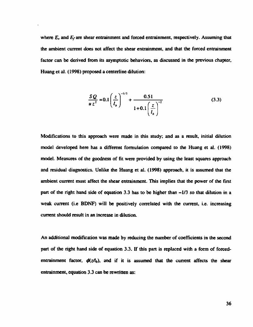
where Es and E1 are shear entrainment and forced entrainment. respectively. Assuming that
the ambient current does not affect the shear entrainment, and that the forced entrainment
factor can be derived from its asymptotic behaviors, as discussed in the previous chapter.
Huang et al. (1998) proposed a centerline dilution:
(3.3)
Modifications to this approach were made in this study; and as a result. initial dilution
model developed here has a different fonnulation compared to the Huang et al. ( 1998)
model. Measures of the goodness of fit were provided by using the least squares approach
and residual diagnostics. Unlike the Huang et al. (1998) approach. it is assumed that the
ambient current must affect the shear entrainment. This implies that the power of the first
part of the right hand side of equation 3.3 has to be higher than -l/3 so that dilution in a
weak current (i.e BDNF) will be positively correlated with the current, i.e. increasing
current should result in an increase in dilution.
An additional modification was made by reducing the number of coefficients in the second
part of the right hand side of equation 3.3. If this part is replaced with a form of forced-
entrainment factor. 1/(zllb), and if it is assumed that the current affects the shear
entrainment, equation 3.3 can be rewritten as:
36

S ~ =e(~]1
+t;(~J u z l, I,
(3.4)
where e and f are model coefficients to be determined based on the data. The forced-
entrainment factor, t/1(1/lb), is formulated by assuming that as 'lllb goes to infinity, equation
3.4 should converge to the advected thermal solution in which the value of the left hand
side of equation 3.4 approaches a constant. This requires that:
as1/lb -+ 0 (3.5)
as 1/lb -+ oo (3.6)
The form of t/l('lllb) that satisfies these requirements is proposed as:
(3.7)
where wand hare model coefficients. Using equation 3.7, equation 3.4 can be written as:
S ~ =e(~]f + wexp (_!!__] uz l, ~
(3.8)
Equation 3.8 is a nonlinear equation so that a nonlinear regression can be employed to
obtain the coefficients (e./. w and h). The least squares approach was used so that estimates
37

( e, j , li· and h ) of the coefficients in equation 3.8 were detennined by minimizing the sum
square error (SS,.,). Given a set of data ( ( :~). { ,: ). ) for i=l,2,3, ... ,n, the sum square
error was formulated as:
ss,.s = t[( s~) - e(.!.)i- w exp r~J ]2
1=1 u z i l b i z{ /lb i
(3.9)
To minimize this, equation 3.9 was differentiated with respect to e, i, w and h. and each
derivative was set to zero, resulting in the following equations:
i J = 0 (3.10) 1=1 U Z I /b i 74 ); /b i
i an(~) ) = o (3.11) 1=1 U Z i lb I '{ lb i lb i
/lb i
![( 5~ J _ e(.!.)i -w exp [.i__J][-exp [.i__J ] = o (3.12) 1=1 uz i lb i z{ z{
/ l, i / lb i
38

Equations 3.10 to 3.13 are also nonlinear in the parameter estimators e , j . w and h .
Therefore, they cannot be solved directly but require some type of iteration process. A
method that is often used in finding the least square estimators in a nonlinear model is a
Gauss-Newton procedure (Myers 1990). Essentially, the procedure is an iterative process
which first e~pands the nonlinear function in equation 3.8 in a Taylor series around a
starting value for the estimators - in this case the estimators are e , j . w and h - and which
retains only linear terms. Thus:
( ) (
W0 J {" .. ) W0 ( ho J + W- W0 exp J4
1
+ 1/t -h, (J4). exp J4 1
(i=l,2,3, ... n) (3.14)
Equation 3.14 can be viewed as a linear approximation in the neighborhood of the starting
values, e0 , io, w0 and h0 • The equation 3.14 can be expressed in the form of:
where OJ ii is the derivative of the nonlinear function (equation 3.8) with respect to the jth
parameter (coefficient). The y i is the jth parameter value minus the starting value. The left
hand side of equation 3.15 can be considered as the residual when the parameters are
39

replaced by staning values. For a given starting value, the (I) ii are known and can be
considered as regressor variables in a linear regression, while the y i plays the role of a
regression coefficient. As a result, the Gauss-Newton procedure builds on the linear
regression structure:
(3.16)
where,
( ) ( )io ( " ) SQ .. Z .. h0 Y; = --z - e0 - -w0 exp --
u z j lb i z{ /lb i
(3.17)
and E; is the enor term of the regression model.
The jth parameter value, i.e. the value of e, j , w and h , can be obtained from an iterative
process as follows:
1. Determine the starting value of the jth parameter, e0 , io, w0 and h0 •
2. Estimate y i in equation 3.16 by multiple linear least squares. Denote these first
iteration estimates by y j.I •
3. Compute the new value of the jth parameter, e.g. e1 = e0 +Y1•1 •
4. Use the jth parameter from step 3 to replace the starting values.
40

5. Return to the first step. and continue the process until converegence is reached
The convergence implies that after. say r iterations. the residual sum squares and
the jth parameter estimates are no longer changing.
This procedure can be carried out using a computer program or available statistical
packages. Applying this procedure, the coefficients in equation 3.8 were determined using
the statistical software SYSTAT from SPSS Science and DAT AFIT from Oakdale
Engineering. Both software packages gave the same answers to third or fourth decimal
places; and for simplicity, second decimal places are given here, i.e. the mean ±standard
enor of 0.13 ± 0.02, -0.31 ± 0.03, 0.46 ± 0.02. and ~.22 ± 0.04 for e, j, w and h,
respectively. The coefficients in equation 3.8 (e, f, w and h) can be replaced with these
estimates by introducing an error term, E, so that the equation 3.8 can be expressed as:
SQ A z A h ( )
j ( ... ) u z2 =e I; +wexp fi. +£ (3.18)
where the error ~nn. ~ is approximately normally distributed with a mean of about zero
and standard deviation of 0.092.
3.5. Model Presentation
The proposed centerline initial dilution can be expressed in detenninistic and probabilistic
forms as shown in equation 3.19 and 3.20, respectively.
41

s z -0.22 ( )
-0.31 ( ) u ~ =0.13 -;;: + 0.46 exp j{. (3.19)
( )
HU1±0.03) (< )) : ~ = (0.13 ± 0.02)
1: + (0.46 ± 0.02) exp -
0·2~ 0·04
+ N (o, 0.092)
(3.20)
where N(O, 0.092) is a random quantity normally distributed with a mean of zero and a
standard deviation of 0.092. This random quantity is basically the error term in the model
given in equation 3.18. The above equations 3.19 and 3.20 are essentially the same except
that equation 3.20 is specified probabilistically containing an error term, E, and uncertainty
measures of the model coefficients, i.e. the mean ± standard error. On the other hand,
equation 3.19 is specified detenninistically to estimate average dilution for a given value of
input varibles. The advantage of using the probabilistic model is that uncenainty associated
with the model itself can be explained. By doing so, the probabilistic presentation can
contribute insight into the reliability of answers given by the model itself for a panicular
situation.
In outfall design, like hydraulic design in general, uncertainty could arise from various
sources, including, but not limited to, data uncertainties, operational uncertainties, and
model uncenainties {Tung 1994, Mukhtasor et al. 1999a). Data uncertainties are associated
with inconsistency, and data measurement and recording enors. Operational uncenainties
42
refer to human factors that are not accounted for in the analysis. Model uncenainties
include the fact that the empirical laws do not describe the complete features of the true
process and that some coefficients in the model cannot be quantified with absolute
certainty.
However, empirical initial dilution models are commonly presented in a detenninistic
fashion without explicitly stating or elaborating the associated uncertainty (e.g. Lee and
Cheung 1991. Wood 1993. Wright 1977a). As a result, applying this deterministic model
may lead to loosing sight of the intrinsic uncertainty associated with the empirical equation.
In that way. much of the infonnation in the data is unused, resulting in unnecessary waste
of information and perhaps flawed design decisions (Tung 1994 ). Therefore, the
probabilistic model becomes a necessary alternative for initial dilution design problems.
This is particularly important because a deterministic solution is only one special case of
many of the probabilistic solutions. which encompass a wide spectrum of possible answers
to a design problem (Tung 1994 ).
Figure 3.2 shows a comparison between deterministic and probabilistic fits of the models
(equation 3.19 and 3.20) to the data. As can be seen from the figure, the deterministic
solution (equation 3.19) provides a single answer for a given value of input variables. For
example, at z/16 of 0.1. SQ/ul is 0.3. On the other hand, the probabilistic solution (equation
3.20) estimates that there is 50% certainty that SQ!ui equal 0.3 when lll, is 0.1. At this l/1,
value, it is also possible to evaluate the probability of getting any possible value of SQ!ui
using the probabilistic model, for example, the probability of having SQ!ui more than 0.5
43
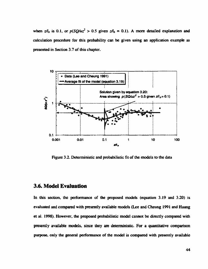
when 1/lb is 0.1, or p(SQ/ui > 0.5 given 11lb = 0.1). A more detailed explanation and
calculation procedure for this probability can be given using an application example as
presented in Section 3.7 of this chapter.
10~----------------------------------------------~
-... ... a. 1
~
• Data {Lee and Cheung 1991)
1 -Average fit of the model (equation 3.19)
Solution given by equation 3.20: Area showing p(SQiuz2 > 0.5 given zll,= 0.1)
0.1 +-~--~~~------~~----~~--~------~------~ 0.001 0.01 0.1 1 10 100
Ill.
Figure 3.2. Deterministic and probabilistic fit of the models to the data
3.6. Model Evaluation
In this section, the perfonnance of the proposed models (equation 3.19 and 3.20) is
evaluated and compared with presently available models (Lee and Cheung 1991 and Huang
et al. 1998). However, the proposed probabilistic model cannot be directly compared with
presently available models, since they are deterministic. For a quantitative comparison
purpose, only the general performance of the model is compared with presently available
44

models, meaning that only equation 3.19 is compared with praently available models.
Figure 3.3 shows a comparison between the Huang et al. (1998) model and equation 3.19.
10~----------------------------------------------~
• Data (Lee and Cheung 1991)
-Huang et al. (1998)
-Equation 3.19
. . . . . . ···············i··················-:···················-=···················;:-.................. .. . . : : : : . . : : .
0.1 +-------~~~----~~--------~------~~------~ 0.001 0.01 0.1 1 10 100
Figure 3.3. Comparison between the Huang et al. (1998) model and equation 3.19
Figure 3.3 shows that the perfonnance of the proposed model is better than that of the
Huang et al. (1998) model. The proposed model gives a less-biased solution in the whole
range of the BDNF, the transition, and the BDFF regions. Compared to the Huang et al.
(1998) model, the proposed model gives higher and lower dilutions for the BDNF and the
BDFF regions~ respectively. The problem of ustructun:d bias" as shown in the previous
chapter is not encountered in the proposed model. For any region, the mean residual of the
proposed model is about zero. The comparison is shown in Figures 3.4 and 3.5.
45

0.3
02
0.1
'iij ~ 0.0 t:) -;; Cl.)
cr -0.1
.02
0.3
02
0.1 1ij ~ t:) -;; Cl.)
0.0 ~
-0.1
-02
--
-
-- I
I I
Translian
Region
I I
BDFF
Figure 3.4. Residuals of the Huang et al. ( 1998) model
-• -
-
- I I -
I I
EIDFF
Region
Figure 3.5. Residuals of equation 3.19
46

From a residual diagnostic, the proposed model has mean values of the residuals of -0.017.
-0.007, and 0.004 for the BDNF. transition, and BDFF. respectively. These mean values
indicate that the model is less biased than the Huang et al. (1998) model, which gives mean
residuals of0.065, 0.021. and -0.050 for the BDNF, transition, and BDFF. respectively.
Furthennore, it can be seen from Figure 3.5 that the spread of residuals is about the same
for all cases, while Figure 3.4 shows that there is a wider spread of residuals in the
transition region. This suggests that, compared with equation 3.19, the Huang et al. (1998)
solution is relatively less precise in the transition region. The accuracy (bias and precision)
comparisons may also be evaluated using a comparison between calculated dilution versus
data, as shown in Figures 3.6 to 3.8. In those figures, a regression equation associated with
the calculated dilution and data is provided for each model. Overall accuracy is also
compared in terms of percentage error of calculated dilution. Statistics of the percentage
error are presented in Figure 3.9.
From Figures 3.6 to 3.8, the perfonnance of the three models can be assessed using the
slope and intercept of the regression equation. For the unbiased model, the slope, intercept
and coefficient ofdetennination, R2, are one, zero, and one, respectively. As can be seen
from those regression equations, all models seem to be acceptable. However, Figure 3.9
provides more meaningful comparative interpretation using the percentage error of dilution,
in which bias measure (mean, median). precision measure (standard deviation, 10- and 90-
percentile). overall accuracy (mean square enor, MSE) are provided. In general, equation
47

3.19 is relatively more accurate as indicated by the lowest value of mean, median, 10- and
90-percentiles, and MSE.
Considering the above comparisons and problems discussed in the previous chapter (i.e. the
conceptual problem. non-unique solution in the transition region, and structured bias),
equation 3.19 is considered to be more justifiable and preferable than presently available
models, i.e. Lee and Cheung (1991) and Huang et al. (1998). The probabilistic fonn of the
proposed model, equation 3.20, is also preferable for initial dilution calculations in
uncertain situations.
121 ~--------------------------------------------------------------------------~ Huang at al. (1998) solution
101 Calculated dilution= 0.019 + 1.08 dilution data R2 = 92.6o/o and s = 6.174
• •• :. ..
• • • •• til!! Une of equality
21
21
• • • • ••• •• • • • • •
41 61 81 101
Initial dilution ...
•
121
Figure 3.6. Comparison between calculated dilution (Huang et al. 1998) and the data
48

121 ~------------------------------------------------~ Equation 3.19:
101 Calculated c:ilution = 1.88 + 0.96 dilution data ~ = 91.3% and s = 6.014
Une of equality A
21
21 41 61 81 101 121
lnttt.l dilution data
Figure 3.7. Comparison between calculated dilution (equation 3.19) and the data
121 ~---------------------------------------------------,
~
.! :i =a
I ~
Lee and Cheung (1991) solution: 101 Calculated dilution = 1.44 + 0.93 dilution data
R2 = 90.9% and s = 5.972
81
61
.s 41 ~
• •
21 •
1 1 21 41 61
Initial dilution c11ta
•
Line of equality
81 101 121
Figure 3.8. Comparison between calculated dilution (Lee and Cheung 1991) and the data
49

c: 0 :;::: .:! :c -0 ... e ... Q)
Q) Cl .f! c: Q)
~ Q) D.
800~------------------------------------------~~------~ Dmean
~ ~~~
600 D 1 0 perct. 090 perct.
500 Dstdev
400 •MSE
300
200
100
0 -+---~==---L---1::::::::1
Huang et al. (1998}
stdev 13.8
MSE 514.7
Lee and Cheung (1991}
15.6
753.0
Equation 3.19
11.3 2.2
14.7 475.8
Figure 3.9. Comparison of percentage error of calculated dilution
It should be mentioned here that the proposed model was developed without taking the data
outliers into account. Figure 3.10 shows the comparison of the models when the outlier
points are included. As can be seen from this figure, there are five points lying far from the
others. As discussed previously, there might be a recording, typing, or calculation error
associated with point #5. It was therefore considered as an outlier and was removed in the
subsequent analysis. In the Huang et al. (1998) paper, treatment of this point was not
discussed.
Points# 1 to 4 seem to be closer to the other data because Figure 3.10 is presented in a log-
log scale. Actually these points are quite far off and affect the least squares solution
50

significantly. The presence of these points results in non-nonnal residuals of the model
using either the approach used in this study or the Huang et al. (1998) model. Removal of
these points improves the nonnality of the residuals. This is shown in Figures 3.11 to 3.14.
Even after removing outliers. the probability plot of the Huang et al. (1998) model gives a
p-value less than the significant level of 0.05 (Figures 3.11 and 3.13) so that the test does
not show that residuals are nonnally distributed. On the other hand. Figure 3,14 shows that
residuals of equation 3.19 are normally distributed with a p-value significantly higher than
the 5% significant level.
10 • Data (Lee and Cheung 1991)
5~ · · · · · · Huang et al. (1998)
-This study
- -~ u4 ell
l I 1
• •• • _...
_....,-.te•• . ··- .•... ···-·· .. • • • •
0.1 . 0.001 0.01 0.1 1 10 100
zll,
Figure 3.10. Influential points producing high residuals in the models
Sl

.998
.91
.95
~ .80 :s .50 as ,Q
~ .20
.05
.01
. 001
Normal Probability Plot
.. I • .•- - .., ~ - .., - 4 • - .., .., - - - - - - - - .., .., .., - - - ,.- • ... , • • - - .., , - - .., -.. ~.2 ~. 1 0.0 0.1 0.2 0.3 0.4 0.5
ttlang et al. Aver.ge: 0.01110301 SlDew: 0. 1~1
~-OM!ng Nom*ity T•t ~2.P-VIIue: 0.11110 N: 1011
Figure 3.11. Probability plot of residuals for the Huang et al. ( 1998) model with outliers
.991
.98
.95
.80
.50
.20
.01
.001
Av.,..: 0.01015t12 SlOw : 0.11.70 N: 108
NomaJ Probabiity Plot
' . ' ' - -.~ - - - - - !'"" - - - - - · - - - - - - -- -- - • - - - - - - • - - - - ·- • - - -
---------------------- - ---·---------------' '
~.2 ~-1 0.0 0.1 0.2
This study 0.3 0.4
...,..,_08111ng NclnNity T•t ~2.:.1 P-V- 0.000
Figure 3.12. Probability plot of residuals for the proposed model with outliers
52
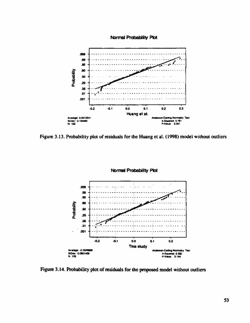
Normal Probability Plot
.119
. 99
.95
• . ----. . -. . ------. ------. --------~ ~ :~ l ~ ~ ~ ~ ... ~ .80 :s .so CD
~ CL
.20
.OS
.01 . . .. ·.---- ... ------.--.---------------.------- ......
. 001
-G.2 -G.1 0.0 0.1 0.2 0.3
Av..-gr. 0.001~1 StOW : 0 .10WM N: 102
1-ltang etal. ~on-O.tng NonM1i1y T•t ~0.711 P-v--= O.lJ't
Figure 3.13. Probability plot of residuals for the Huang et al. (1998) model without outliers
Normal Probability Plot
.991
.98
.95
~ .110 :a .so CD
l .20
.OS -- : -. r- --.. -- --. -·.---. -------- ----~ ----- -. . .
. 01 - -. ~ -- - - - - - ~ - - - - - - - -:- - - -- - -- ~ - - .. - - - ...... - - - - -.ocn --~-------~-------~-----------------------
Av..-gr. -o.~ SlOW: O.C*l1451 N: tal
.0.2 -G.1 0.0 0.1 0.2
This study Alldllaon-O.tng Narrnality T•l
--~0.510 p.v..._ 0.1 ..
Figure 3.14. Probability plot of residuals for the proposed model without outliers
53

From the above discussions, it may be stated that a nonlinear regression modeling
combined with a length scale analysis is a promising approach for modeling initial dilution.
This study suggests that experimental work on dilution analysis may be usefully
supplemented with a suitable data analysis. The approach discussed in this chapter may be
useful for such a purpose.
3.7. Appticadon Example
An example of an application is presented here using a case, which characterizes many
operating outfalls, taken from Lee and Cheung (1991). The example considers a single pon
buoyant jet from an ocean outfall with a diameter (d) of 0.5 m, an initial jet velocity (uj) of
0.6 m/s, a relative density difference ratio of 0.026, and a seawater depth above the
discharge (z) of 10m. With this situation, the outfall has a depth to diameter ratio (z/d) of
20. The volume, momentum, and specific buoyancy fluxes are computed to be 0.1178
m3/s, 0.0707 m4/s2, and 0.03 m4/s3
, respectively: With relevant length scales IQ and lM of
0.44 m and 0.79, respectively, relative to the depth, both the source geometry and the initial
momentum are not significant, that is, z >> IQ and z >> IM.
In order to evaluate the dilution in different regions, i.e. the BDNF, the transition, and the
BDFF, three values of ambient current speed. u, are specified at 0.025, 0.1, and 0.3 m/s.
This results in different buoyancy length scales, lb of 1920, 30, 1.1 m, respectively. and the
ratio of depth to buoyancy length scales, zll,, of 0.00521 (BDNF), 0.33 (transition), and 9
(BDFF)! respectively. For the asymptotic solution (Lee and Cheung 1991). centerline
54
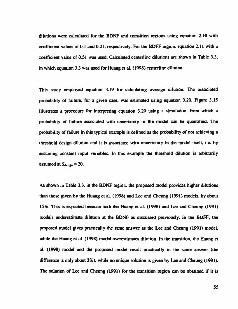
dilutions were calculated for the BDNF and transition regions using equation 2.10 with
coefficient values of 0.1 and 0.21. respectively. For the BDFF region, equation 2.11 with a
coefficient value of 0.51 was used. Calculated centerline dilutions are shown in Table 3.3.
in which equation 3.3 was used for Huang et al. (1998) centerline dilution.
This study employed equation 3.19 for calculating average dilution. The associated
probability of failure, for a given case, was estimated using equation 3.20. Figure 3.15
illustrates a procedure for interpreting equation 3.20 using a simulation, from which a
probability of failure associated with uncertainty in the model can be quantified. The
probability of failure in this typical example is defined as the probability of not achieving a
threshold design dilution and it is associated with uncertainty in the model itself. i.e. by
assuming constant input variables. In this example the threshold dilution is arbitrarily
assumed at Sdrsirn = 20.
As shown in Table 3.3, in the BDNF region, the proposed model provides higher dilutions
than those given by the Huang et al. (1998) and Lee and Cheung (1991) models, by about
15%. This is expected because both the Huang et al. (1998) and Lee and Cheung (1991)
models underestimate dilution at the BDNF as discussed previously. In the BDFF. the
proposed model gives practically the same answer as the Lee and Cheung (1991) model.
while the Huang et al. (1998) model overestimates dilution. In the transition. the Huang et
al. (1998) model and the proposed model result practically in the same answer (the
difference is only about 2%), while no unique solution is given by Lee and Cheung (1991).
The solution of Lee and Cheung (1991) for the transition region can be obtained if it is
55

assumed that it can be calculated using the BDNF equation with a modified coefficient ( C 1
= 0.21 ), resulting in different results of about 27%.
Table 3.3. Comparison of estimated centerline dilution among different models
Case I Region lee and Cheung (1991) 1 Huang et al. (1998)2 This st~. S(p,)
1 BDNF 12.2 12.2 14.1 (0.943)
2 Transition 25.8 34.9 35.6 (0.022)
3 BOFF 129.9 142.0 131.1 (0.000)
1Calculaaed using equaaions 2.10 and 2.11 2Calculated using equation 3.3 3Calculated using equation 3.19. The value in the brackels is lhe probability of failure (p1). for which a calculation procedure is outlined in Figure 3.15.
Furthermore. the proposed model can be used to evaluate the reliability of the model by
calculating the probability of not achieving a threshold design dilution for a given discharge
scenario. If the threshold is set at sd~s;gn = 20, for example, then the probability of failure is
94.3%, 2.2%, 0% for cases where the ambient current speed, u, is at 0.025, 0.1. and 0.3 rnls.
respectively. On the other hand, using the deterministic approach without considering
uncertainties in the model (e.g. Lee and Cheung 1991 and Huang et al. 1998), the resulting
dilution calculation would always correspond to a 50% failure probability.
56

Define problem: hydrodynamic characteristics
values of input variables threshold value of initial dilution
number of simulation (ns)
Set initial values (f= 0, r = 0)
Generate a random value from the normal distribution for the model coefficients and error term,
with associated mean and standard deviation
Calculate centerline dilution using equation 3.19
No
Probability of Failure, p, = fins
Figure 3.15. Flow chart of the procedure of evaluating probability of failure associated with model uncertainty.
57

3.8. Summary
A new approach to modeling initial dilution was proposed in this research. It was based on
the hypothesis of additive shear and forced entrainment combined with nonlinear
regression. The least squares approach and the Gauss-Newton numerical analysis were
employed in this study. Unlike a previously available approach, which is typically "'trial
and ertor''. the proposed approach provides an objective means of evaluating the model
performance. Using the proposed approach. an alternative initial dilution model, which is
more robust. is presented in this chapter. The model provides an unbiased solution for the
whole range of the BDNF. the transition, and the BDFF. It gives a unique, continuous.
solution of centerline dilution, which is presented in equation 3.19. A probabilistic form of
the model is also given in equation 3.20. An example of an application tor both
deterministic and probabilistic evaluation of initial dilution is also provided.
Comparison of the proposed model with other available models shows that the proposed
model is better in a number of ways: ( 1) it does not assume that the current has no effect in
the BDNF. which asymptotic solutions do; (2) in the BDFF region the model has one
parameter fewer than the Huang et al. (1998) model yet it is no less accurate; (3) in the
transition region it gives a unique solution which the asymptotic models do not; (4) unlike
the Huang et al. (1998) model, the proposed model has approximately the same precision
for all regions, i.e. the BDNF, the BDFF. and the transition; and (5) the proposed model can
also be presented in a probabilistic fonn that permits calculation of failure probability for
specified model inputs and a threshold dilution.
58

Chapter4
Hydrodynamic ModeHng: Deterministic and Probabilistic Analyses
4.1. Introduction
Concepts of hydrodynamic modeling and the importance of initial dilution as an element of
the modeling have been presented in Chapter Two. An alternative model for initial dilution
in the near field has been proposed in Chapter Three. This chapter discusses the integration
of near field and far field modeling, and an approach to evaluate the intermediate region
between the near and far fields. Hydrodynamic modeling of typical mixing processes,
which can occur as a result of discharging produced water into a marine environment, is
presented in this . chapter using deterministic and probabilistic analyses. Previous work
related to hydrodynamic modeling of effluent discharges is reviewed in light of its
application in the case of produced water discharge. Focus is directed at evaluating
uncertainty associated with modeling and methods of dealing with this uncertainty. This
chapter also describes an integrated hydrodynamic model using a detenninistic approach. A
methodology of probabilistic hydrodynamic modeling is then presented. An application
59

example based on available information relevant to a typical offshore discharge of
produced water is discussed in these sections.
4.2. Context
Hydrodynamic modeling using quantitative methods has been the most important tools for
outfall design and environmental assessment purposes. Some of the quantitative methods
have become quite elaborate and include sophisticated analysis; however, irrespective of
the level of sophistication in the models, including experimental models, they are
developed under some assumptions that simplify the problems. Consequently, they might
not reflect the actual conditions of the problems under investigation and are assoc1ated with
some degree of uncertainty. Furthermore, people have rarely provided complete
information, such as values of parameters and uncertainties in data.
One cannot predict with certainty the occurrence (or nonoccurrence) of specific event. The
underlying uncertainty may be due to: a) the inherent randomness of the natural
phenomenon, b) the inaccuracies in estimating the parameters and in choosing the
distribution. and c) the inaccuracies of modeling, which is based on idealized assumptions
(Ang and Tang 1975). As a result. the use of a deterministic approach. which does not
explicitly take these uncertainty factors into account in solving engineering problems.
although sometimes useful. may in some cases lead to unrealistic results. This may result in
a partial loss of infonnation~ misleading results. and incorrect solutions. Properly, the tools
60

of engineering analysis should therefore include methods and concepts for evaluating the
significance of uncertainty on system perfonnance and design (Mukhtasor 1998).
In hydrodynamic modeling, uncenainty may be associated with a number of different
factors, including uncertainty in model fonnulations and model inputs. Many model inputs
used in hydrodynamic modeling, e.g. seawater current speeds and directions, are highly
variable. In addition to this, as discussed in the previous chapter, model fonnulation may
pose some degree of uncertainty, which may in pan be reflected by uncertainty of its
coefficients. However, hydrodynamic modeling of the discharge of produced water is
unable to deal quantitatively with these uncertainties (e.g. Smith et al. 1996, Somerville et
al. 1987). Previous efforts of modeling typically use simplified models (e.g. Rye et al.
1996) and assume a worst-case scenario by looking at dilution at 500 m from the platfonn
(Kannan and Reerink 1998). Other approaches of modeling are also deterministic in nature,
such as the use of buoyant jet fonnulation (e.g. Skatun 1996) or far- field dispersion
modeling (e.g. Murray-Smith et al. 1996).
Considering a worst-case scenario without explicitly taking uncenainty into account, a
deterministic approach is compelled to rely on conservative assumptions. When these
assumptions are compounded in estimating toxic chemical concentration, for example, the
result becomes even more conservative, and can lead to misplaced control activities and
environmental management priorities (Finley and Paustenbach 1994 ). In this context,
presently widely used deterministic approaches need to be complemented by a probabilistic
analysis. Results of a probabilistic analysis should help risk managers to make explicit
61

decisions about how conservative their recommendations are (Finley and Paustenbach
1994).
4.3. Near Field ModeUng
Hydrodynamic mixing of the effluent discharge in the near field, or initial dilution, can be
increased by the proper design of the geometry of the outfall for specified characteristics of
the effluent and ambient seawater. This includes selection of the shape, size and
arrangement of effluent outlet, which may consist of a simple open end (single port) or a
multipart diffuser containing a regularly spaced line of relatively small pons. This Section
considers near field modeling of a single port discharge into a marine environment. The
reason for choosing the single port type is discussed in Chapter Six (Subsection 6.4.2).
The near field mixing presented in the previous chapters is applicable for a deep-water
condition, in which a distinct buoyant jet rises to the surface and dilution occurs because of
turbulent jet entrainment (Jirka and Lee 1994 ). Upon impingement on the free surface, the
effluent plume spreads laterally in the form of a stable density current (Hamdy 1981 ). A
criterion for a deep-water condition is defined as:
H - > 0.221;, d
(4.1)
62

where H is the depth of receiving water, and d is the diameter of port. Fo is the densimetric
Froude number, which is defined as (William 1985):
(4.2)
Equation 4.1 has little sensitivity to the discharge angle (Jirka and Lee 1994). When this
criterion is not satisfied, the discharge falls in the category of shallow water condition. in
which the discharge momentum may be sufficiently strong to cause a dynamic breakdown
(instability) of the buoyant jet motion and create a local circulation zone as shown in Figure
4.1 (modified from Hamdy 1981). In order to maximize the dilution, unstable discharge is
typically avoided because of recirculation of the plume and limited entrainment into the jet
(Hamdy 1981).
For stable discharges, Chapter Two defines the concept of initial dilution and discusses
problems associated with presently available initial dilution models. A unique, continuous.
initial dilution model, which was derived from experimental data covering conditions of
many operating ocean outfalls, including produced water outfalls, is presented in Chapter
Three. The model is suitable for a round buoyant jet, i.e. discharge from an open-ended
outfall into unstratified moving waters. The deterministic and probabilistic formulations of
the initial dilution model are rewritten in equations 4.3a and 4.3b, respectively.
63

Figuxe 4.1. Various discharge characteristics (Top: stable, deep water discharge, middle: transition discharge, and bottom: unstable, shallow water discharge)
64

SQ z -0.22 ( )
-().31 ( ) u z, =0.13 /; + 0.46 exp }{. (4.3a)
( )(~.31± 0.03) ( J : ~ = (0.13± 0.02)
1: + (0.46 ± 0.02) exp (-
0·2}(
0·04
) + N(O, 0.092)
(4.3b)
where Sis the initial (centerline) dilution (dimensionless) at an elevation z above discharge;
Q is the outfall discharge rate. u is the ambient cunent speed (m/s); N(O, 0.092) represents
residuals of the model that are normally distributed with a mean of zero and standard
deviation of 0.092; and lb is the buoyancy length scale defined as:
(4.4)
in which g is the gravitational acceleration; Pa and Po are the densities of the ambient
seawater and effluent, respectively.
Lee and Neville-Jones (1987a) provide a useful modeling approach to estimate the
trajectory of the buoyant jet. For a typical horizontal discharge, the motion in the horizonlal
(x·y) plane is driven by the jet momentum, M, and the ambient current, u. Since the
discharge imparts no vertical momentum, the motion in the vertical (x·z) plane is
65

determined primarily by the interaction of the discharge buoyancy and the ambient flow.
The trajectory equations have been reported in the literature (e.g. Lee and Neville-Jones
1987a. Wright 1977b) and models for the horizontal boil location xb at the seawater surface
can be written as:
for H <<lb (4.5)
for H >>lb (4.6)
where H is the water depth above discharge, and C J and C4 are coefficients determined
based on field and laboratory data. Huang et al. (1996) proposed an interpolation method to
deal with the nonlinearity in the transition between the two cases (equations 4.5 and 4.6). In
this interpolation method, equations 4.5 and 4.6 are used within the region of Hll, <0.1 and
>10, respectively. Between these two ranges, the value of a variabl•! is a function of those at
other regions, defined as:
(4.7)
where Io.r • Iro and Irr are regional variables for HA, <0.1, HA, >10, and 0.1~ HA, ~ 10,
respe<:tively. The coefficients a1 and a2 are estimated from (Huang et al. 1996):

a,= 0.5-0.Siog,{ ~) (4.8)
a.,=0.5+0.51og1{ ~) (4.9)
Wright (1977b) reponed values of C3 (equation 4.5) that depend on the method of obtaining
the da~ i.e. 0.6702 from photographic measurements and 0.4571 from concentration
measurements. Huang et al. (1996) used a value of 0.5824 for CJ based on the CORMIX
model (Doneker and Jirka 1990). From Wright (1977a). a variation of CJ from typical
photographic measurements is in the range of 0.5 17 to 1.494.
While CJ is usually treated as a constant. it seems that there is no common agreement
whether c., (equation 4.6) is a constant or a variable that depends on other physical
quantities. Lee and Neville-Jones (1987a) proposed a value of c., of 1.1 for estimating time-
averaged boil location Xb based on field experiments at six outfalls. However, Wright
( 1977b) noted that c., varied depending upon the ratio of the buoyancy and momentum
length scales i.e.
( ),, ..
c.= c, :: (4.10)
where l,. is defined as:
( )
Ill
" -Q I = --~---• "
(4.11)
67

Values of C5 also depend on the method of obtaining the dat~ i.e. 0.6037 and 1.2761 based
on data from photographic and concentration measurements. respectively.
A constant value for c., might be acceptable for a site-specific outfall condition with a small
variation in the ratio of the buoyancy and momentum scales (equation 4.10). Furthermore.
it is not uncommon practice to treat C4 as a constant. In produced water modeling. for
example. this practice has been adopted by employing the CORMIX model (Smith et al.
1996), in which the value of C4 is taken to be 1.0 (Huang et al. 1996, Doneker and Jirka
1990). Whether or not c, is actually a variable is one problem. Even if it is assumed to be a
constant. there is uncertainty in defining its value. which is another problem. From the
Wright (1977a) experiments. values of c., are typically in the range of 0.2254 to 1.7075.
Methods of dealing with this uncertainty are discussed in Section 4.6.
4.4. Intermediate Mode6ng
Completing the plume rise in the near field region. surface impingement takes place. The
jet is deflected and begins to spread horizontally. The process may result in the phenomena
of the boil and the hydraulic jump. if a jump occurs. A control volume. which is a region
where the surface impingement takes place. can be defined as the intermediate region.
which connects the near and far fields. Figure 4.2 provides a schematic definition of the
intermediate region (modified from Doneker and Jirka 1990).
68

Side View
(a) Near-horizontal plume
I ~,__Plume
Centerline
Side View ! I
Plan View
(b) Near-vertical plume
H
Figure 4.2. Typical inlermediate region of discharges
For typical produced waler modeling, the intermediate region has been neglected.
Somerville et al. (1987), for example, adopted the Brooks (1960) model as a far field
dispersion model. The inputs of the model are taken direcdy from the output of the initial
69

dilution model. Smith et al. ( 1996) used a similar approach to that of Somerville et al.
(1987): modification of the initial dilution outputs, before running into the far field
dispersion model, is not carried out in these cases.
Formulation for the analysis of the intermediate region is available in the literature
{Doneker and Jirka 1990. Wright et al. 1991 and Huang et al. 1996). These are based on a
control volume approach, in which the inflow is the rising buoyant jet flow near the water
surface and the outflow is the surface plume that is advected by the ambient cunent. The
outflow characteristics required for connecting the near and far fields include the bulk
dilution Sa (or alternatively the pollutant concentration of interest Ca. where Ca = Cr/Sa. and
Co is the pollutant concentration in the effluent prior to discharge), the plume width L0 , the
plume thickness hl'h and the distance from the boil center to the upstream (L:~) and
downstream end of the control volume (x0 ). The formulations proposed by Doneker and
Jirka (1990) and Huang et al. (1996) have been partly calibrated for typical field tests of an
outfall plume. The deterministic components of these formulations are considered in this
study for further modification into a probabilistic analysis of hydrodynamic modeling.
4.4.1. Bulle dilution
The bulk dilution at the downstream end of the control volume, Sa. is estimated
(Wright et al. 1991, Doneker and Jirka 1990, Huang et al. 1996) as:
Sa= Cs1 S
Sa= Csz S
forHAb <0.1
forHAb > 10
(4.12)
{4.13)
70

When HAb < 0.1, the rising buoyant jet is only weakly deflected by the ambient cunent and
approaches the water surface at a near-vertical angle. In this case. an internal hydraulic
jump is expected to occur. As relevant experimental data is unavailable, the coefficient Cs1
is typically estimated based on experiments in stagnant water (Wright et al. 1991. Huang et
al. 1996). This assumption. i.e. the applicability of a stagnant water experiment to a case
with a weak ambient current. poses some degree of uncertainty, which is unquantifiable.
Only the uncertainty associated with values of the coefficient Cs1 may be quantified by
specifying its values between 3 and 5 based on experiments from Wright et al. (1991).
When H/16 > 10, the rising buoyant jet is strongly deflected by the ambient current and
approaches the water surface at a near-horizontal angle. The flow is advected with the
ambient velocity at the speed u of the surface plume layer. For this case, the constant CS2 in
equation 4.13 is reported to be in the range of 1.5 to 2.0 (Doneker and Jirka 1990, Huang et
al. 1996). Typical field test-based calibrated values of the coefficients are 2.01 and 1. 74 for
Cs1 and CS2, respectively (Huang et al. 1996).
4.4.2. Pl11me width and 11pstream intnlsion length
The plume width at the downstream end of the control volume, Lo. is estimated
(Doneker and Jirka 1990, Huang et al. 1996) as:
£., = 5.2 Ls for Hllb < 0.1 (4.14)
71

where Ls is the upstream intrusion length, which is the distance from the boil center to the
upstream end of the control volume. For this case (i.e. H/111 < 0.1 ), the parameter L.f is
defined (Akar and Jirka 1994b, Doneker and Jirka 1990) as:
Ls = 2.12 H312 (I-eos 6)312 1,-113 for 1,/H > 6.11(1- cos 6) (4.15a)
Ls = 0.381, for 1,/H s 6.11(1 -cos 6) (4.15b)
where 6 is the angle between the rising buoyant jet axis and the water surface. estimated
from 6 = tan"1(Hix,) (Huang et al. 1996).
When HR, > 10, the plume width at the downstream ~nd of the control volume, Lo. and the
distance from the boil center to the upstream end of the control volume. Ln are estimated
from equations 4.16 and 4.17, in which an equivalent cross-section aspect ratio for the
outflow section of 2: 1 is assumed (Doneker and Jirka 1990, Huang et al. 1996).
L=-·-r·Q .. sin8 tr u
forHII, > 10
forHII, > 10
4.4.3. Disttmee of downstre11111 entl and plume thielmess
(4.16)
(4.17)
The distance from the boil center to the downstream end of the control volume, xlh
is estimated by assuming that it is proportional to the depth above discharge, H, defined as:
72

xo=CDI H
xo=Co2H
forHA, <0.1
forHA, > 10
(4.18)
(4.19)
where C01 and C02 are model coefficients. The value of Cor is typically set at 3 (Huang et
al. 1996. Wright et al. 1991) and C02 at 0.6 (Huang et al. 1996, Doneker and Jirka 1990). In
any case, the plume thickness ho can be estimated from the continuity equation as:
(4.20)
4.4.4. Transitional regime
Characteristics of interest discussed above are defined as the regional solutions, i.e.
in the regimes of HA, < 0.1 and HA, > 10. To have a smooth transition between these
regimes, the same treatment interpolation method defined in equations 4. 7 to 4.9 are
applied as suggested by Huang et al. (1996). That is, a solution for a characteristic in the
transitional regime (0.1 s HA, s 1 0) is taken to be a linear combination of the solutions of
the other two regimes for that characteristic with a formulation presented in equation 4. 7.
Values for the characteristics Sa.· Lo and ho discussed in this section are then taken as the
initial condition for the far field modeling.
73

4.5. Far Field Modeting
Hydrodynamic mixing of an effluent plume and ambient seawater in the far field is largely
governed by two mixing mechanisms: buoyant spreading and turbulent diffusion. Buoyant
spreading refers to a self-driven plume dispersion process. in which the buoyancy residual
contained in the plume promotes the vertical collapse and horizontal transverse spreading
of the plume. In addition to this self-driven process, oceanic turbulence disperses the
effluent plume. This later process is referred to as turbulent diffusion. Both buoyant
spreading and turbulent diffusion may be present in the dispersion processes of the effluent
plume in the ocean; however, the relative imponance of each mechanism depends upon the
characteristics of the discharge and ambient waters (Akar and Jirka 1994a, Huang and
Fergen 1997).
Typical field tests of outfall plumes indicate that the effluents were dominated by buoyant
spreading over a range of severa1 hundred meters from the outfall (Hazen and Sawyer
1994). Such spreading processes result from the buoyancy forces caused by the density
difference of the mixed flow relative to the ambient density. If the discharge is not buoyant,
or is weakly buoyant and the ambient is unstratified, there is no buoyant spreading
(Doneker and Jirka 1990). This is, however, not the case for most produced water
discharges as discussed in Chapter Two.
One approach to produced water dispersion typically neglects the buoyant spreading
without evaluating whether or not the residual buoyancy is significantly absent (e.g.
74

Somerville et al.l987, Washburn et al. 1999). A deterministic far field analysis of
dispersion processes considering the residual density difference is provided in the new
version of the Offshore Operators Committee (OOC) model (Brandsma et al. 1992). The
OOC model was developed analytically by employing mathematical models of
conservation of mass, momentum. and energy.
A simpler fonnulation than the OOC model has been proposed by Doneker and Jirka
(1990) and was implemented in the CORMIX model. The CORMIX model is widely used
for offshore discharge analysis (e.g. Huang et al. 1996, U.S. EPA 1997) and was calibrated
using many sets of laboratory and field data (Doneker and Jirka 1990. Huang et al. 1996).
Figure 4.3 shows a sketch definition of a typical buoyant spreading process (modified from
Doneker and Jirka 1990 and Huang et al. 1996). Typical model formulations for the
spreading can be rewritten as:
h(x)= h,( Lt r (4.21)
L(x) =c.. ( 3P [ ~.r:. + l' (4.22)
where a is the entrainment coefficient ranging from 0.15 to 0.6. with a typical field test
calibrated value of 0.59 (Huang et al. 1996, Doneker and Jirka 1990), /3 is the model
constant ranging from 0.707 to 1.414, with a typical field test calibrated value of 1.33
75

(Huang et al. 1996, Doneker and Jirka 1990), lb is the buoyancy length scale, typically
evaluated for current speed at the S m depth (Hazen and Sawyer 1994 ), x is the distance
along the plume centerline and x = 0 is set at the center of the downstream end of the
control volume, and L(x) is the plume width. The parameter L(x) is assumed to be related
to the standard deviation cr(x) of the concentration distribution across the plume width by
L(x) = 2(3)112cr(x), being consistent with Brooks (1960).
y
-----~ ~I
~l"'iiiil
" Initial Condition
Plan View
.. 1 1.. Frontal zone v ~ =t.-~;~-5 I H
I I
I ~
Cross-section A-A
Figure 4.3. A typical sketch definition of buoyant spreading
76

Dilutions, or pollutant concentrations, associated with buoyant spreading processes are
typically estimated by assuming that the concentration of a tracer in the surface plume has
an error function distribution across the plume width and a uniform distribution across the
plume thickness. Based on these assumptions and a mass balance, the pollutant
concentration at a point (x, y) is estimated (Huang et al. 1996) as:
C(x, ) = 1.832 C ~ .!.[eJ 0·273 Lo + y) + e.J 0•273Lo- y)] for X 2:0 (4.23) y 11 h(x) 2 'J l J2 a(x) "J l J2 O'(x)
where y is the horizontal coordinate perpendicular to the other horizontal coordinate x
(which is along the plume centerline), Ca is the bulk pollutant concentration at the
downstream end of the control volume (x = 0) estimated from the associated bulk dilution
(equations 4.12 and 4.13), erj() is the error function defined as:
2 w : erf(w) = c J e-" dv
'lt/Tr 0
(4.24)
The error functio~ can be solved approximately using Simpson's rule (Markham 1993). The
function can also be evaluated from a statistical table of the area under the Nonnal
Distribution curve by a change in variable such that (Williams 1985):
erf(w) = 2 A(z) (4.25)
77

where z = 1.414 w, and A(z) is the area of the Standard Normal Distribution from 0 to z
along the abscissa.
As indicated, equation (4.23) may only be used for x ~ 0, otherwise it must be modified. It
is typically assumed that the concentration is zero when x < (-Ls- xo). When (-xo + Ls) <
x < 0 the concentration is 1.2 Ca to be consistent with Huang et al. (1996). The average boil
concentration [CJ(1.7 S)] is defined when (-Ls- xo) s x s (-xo + Ls). where C, is the
concentration prior to discharge and Sis the centerline initial dilution (Hazen and Sawyer
1994, William 19985). A parabolic shape defined by Akar and Jirka (1995b) is adopted in
this study to formulate a relationship of the width and the distance of the plume within
( -Ls - xo) s x <0 such as:
(4.26)
This type of deterministic hydrodynamic model that assumes buoyant spreading has been
calibrated based on data from laboratory and field tests, e.g. field tests on outfall discharges
in the South Florida marine environment (Huang et al. 1996). The model is intended to
estimate hydrodynamic characteristics of the plume in the vicinity of the discharges, in
which effects of turbulent diffusion are less dominant than those of buoyant spreading. This
approach may be valid only for a distance relatively close to the discharge. As the
spreading plume travels downstream, the buoyancy effects gradually diminish, and at a
particular distance the ambient turbulence of the receiving water is more dominant in the
78

mixing process (Akar and Jirka 1995a). A criterion to characterize this transition is
typically set by using the flux Richardson number R1 which may be approximated from
(Akar and Jirka 1994a~ Doneker and Jirka 1990):
(4.27)
where K is von Kannan constant~ with a value of 0.4. h is the plume depth. u. is the shear
velocity, and g' is the reduced gravitational acceleration defined as:
(4.28)
R1 can be used as a criterion in employing far field hydrodynamic models. i.e. buoyant
spreading or turbulent diffusion models. When R1 falls below some critical value R~r the
buoyancy effects become relatively unimportant. Critical values of R1 between 0.1 and 0.2
have been reported from experimental tests, and an average value of 0.15 is typically
adopted (Akar and Jirka 1994a).
It should be noted here that although the models formulated in this chapter may be
applicable for only a limited case, i.e. relatively close to the discharge location, they are
useful for evaluating discharge scenarios of produced water from offshore platforms.
Despite the fact that there are field variations in produced water effects~ studies show that
ecological effects of produced water can generally be associated with the distance from the
79

outfall and that the effects are usually limited close to the discharge location (within 500 to
1000 m radii). This may be because of rapid dilution in the marine environment (Frost et al.
1998, Somerville et al. 1987, Stromgren et al. 1995). Besides that, the design of the
discharge scenario is usually directed at evaluating regulatory ambient water quality criteria
which are in tum typically specified using a mixing zone concept, e.g. about 100 m or 200
m from the discharge location. It is obvious that if the analysis is extended in the range
larger than that considered in this study, both of the phenomena (i.e. buoyant spreading and
turbulent diffusion) may have to be considered for the problem of interest.
4.6. Integrated Model
The models discussed in the previous sections are detenninistic steady state models based
on physical principles. Local concentrations of produced water near an ocean outfall
following a discharge may vary continuously both in space and time, mainly due to
variability of ocean currents that advect the effluent plume. To simulate the variation, a
coordinate system defined by Huang et al. (1996) is shown in Figure 4.4. This coordinate
definition can be used to locate and simulate plume movement around the outfall discharge.
In that figure, a fixed global coordinate system X. Y is defined; X is to the right (horizontal
direction), Y is to the top (vertical direction), and the origin is set at the outfall location. A
translating local coordinate system x.y for the surface plume is defined so that it varies
depending on the variation of governing parameters, such as ambient current speeds and
directions. A transfonnation between the translating coordinate system and the fixed
coordinate system can be defined as:
80

x = X cos t/) + Y sin t/) - xb - xo
y = Y cos t/) - X sin t/)
(4.29a)
(4.29b)
where t/) is the current direction (radian) with respect to the X -coordinate direction.
If simulated concentrations at points of concern can be assumed to be a representative
sample of produced water concentrations. a simulated concentration field at an instance
may be regarded as one possible "snapshot .. of an outfall plume. The concentration field
can be defined by dividing an area around the outfall into grids (Figure 4.5). Concentration
at every grid point is calculated by employing near. intennediate, and far field models
discussed above. By doing this, the model may be regarded as a quasi steady state model.
X
Figure 4.4 Coordinate definition for locating plume movement
81

200U • • • • ••• • • • • 4
• • • • • ••• • • • • 4
100 • • • • • ••• • • • • • I • • • • • ••• • • • • l i • • • • • ••• • • • • - 0 • • • • ••• • • • • t .. • • • • ••• • • • •
4 • • • • ••• • • • • -100 I • • • • ••• • • • • •
I~ • • • • ••• • • • • • -200 • • • • • ••• • • • • 4 •
-~._----~-.---4-~~----4H~~.-~~~---4~------
-300 -200 -100 0
X(ID)
100
Figure 4.5. Typical grid points showing nodes for the simulation
300
An application example of an analysis is presented here by considering a hypothetical study
associated with a potential discharge of produced water from an offshore platform on the
Grand Banks, southeast of St. John's, Newfoundlan~ Canada (Petro-Canada 1996,
Mu.khtasor 2000, Mukbtasor et al. 2000c). The focus in this analysis is to show a potential
application of the methodology outlined above using a deterministic approach. A
comparison is given using a presently available model, i.e. the CORMIX model (Jirka et al.
1996), which is recommended for use for a typical dilution analysis of produced water
(U.S. EPA 1997).
82

For this purpose, consider a potential discharge of produced water with a flow rate of
approximately 0.212 m3/s~ and a relative density difference of about 0.025. A discharge
design is specified with a single port located about 11 m below the sea surface. With these
parameters, hydrodynamic characteristics of the discharge would likely be in the range of
those calculated based on data from other produced water discharges worldwide (Brandsma
and Smith 1996, Smith et al. 1996, and Somerville et al. 1987). Using this information.
simulations were carried out using the methodology discussed above and the concentration
distribution up to 300 m downstream is shown in Figure 4.6.
This study estimated that the far field dispersion region begins at about 22.9 m downstream
from tht: boil location, with the centerline effluent concentration at the edge of the mixing
zone, 100 m downstream, of approximately 2.3% and average effluent concentration of
about 1.4%. The CORMIX model (DOS version 3.20, Jirka et al. 1996) was also used in
this study; and its typical plume evaluation result is graphically shown in Figure 4. 7. The
CORMIX model estimated the edge of the near field region to be at 23.5 m downstream,
with an average effluent concentration at the edge of mixing zone, 100 m downstream, of
approximately 1.5%. The comparison shows that the two approaches are generally in good
agreement, particularly in estimating average effluent concentrations.
It should be noted here that the scale of the horizontal axis in Figures 4.6 and 4. 7. are
different because of restriction in the CORMIX model, in which the horizontal distance
must be specified at least 100 times the average depth. H the depth of the water at the Grand
Banks site is about 80 m, for example, the minimum horizontal distance that has to be
83

specified in the CORMIX model is at least 8 km, which is typically beyond the distance of
interest in the case of produced water discharge. To manipulate this restriction, the water
depth of 15m, i.e. 4 m below the discharge port, and the horizontal distance of 2 km were
specified for the CORMIX simulations.
E
>
-50
-100
-150
-200
-25
·300+---.----.---,----,---,----,---,----,---.----.---.----+ -300 ·250 -200 -150 ·1 00 -50 0 50 100 150 200 250 300
X (m)
Figure 4.6. Concentration distribution (% ), a plan-view of the produced water plume.
84

13ran" Bank Produced" water " dLscharge" scenario" Nl
i
CORMIXl Pred1ction File: sLm '-. l"luktasor.cxl
............................................................................................................................................
~ I
0 iOO 800 1200 1600
Plan Uieu 2000
X (Jn)-
Help
Quit
Figure 4.7. Typical CORMIX output, a plan-view of the produced water plume
In contrast to the methodology presented here, the CORMIX model provides only averaged
concentrations at different distances downstream, even though the width of the plume can
typically be as much as about 65% of the downstream distance as shown in Figures 4.6 and
4.7. Furthermore, since a regulatory mixing zone may also be defined in terms of horizontal
area (Doneker and Jirka 1990, Huang et al. 1996), the distribution of effluent concentration
in both X- and Y-directions are important to analyze so that the area of impact zones can be
estimated. In this situation, the approach employed in this study, which provides
concentration distribution in the horizontal (X-Y) plane, is more appropriate, particularly
when this is combined with an analysis of plume location around the boil as a result of
85

variation of ambient current speeds and directions. In addition. the approach described here
is readily modified into a probabilistic analysis to estimate. for instance, concentration
distributions or exceedance probability fields for prescribed threshold toxic concentrations.
Uncertainty associated with modeling can also be evaluated for better assurance of the
reliability of the modeling as discussed in the following section.
4. 7. Probabilistic Analysis
The immediate objective in a probabilistic analysis is to present a systematic approach to
deal with uncertainty, which is inevitable in hydrodynamic modeling. The tenn uncertainty
is sometimes associated specifically with partial ignorance or lack of perfect infonnation
and it is different from variability (U.S. EPA 1996a. Frey and Burmaster 1999). In other
cases, like in this study, the term uncertainty may also be used to refer to either variability
or lack of perfect infonnation about phenomena or model variables (Ferson et al. 1999,
Mukhtasor et al. 1999a). Variability represents diversity or heterogeneity in a well
characterized population, and is a property of nature and usually not reducible through
further measurement or study (Frey and Bunnaster 1999). It may include temporal and
spatial variation, and heterogeneity among individuals (Ferson et al. 1999). For example. at
different seasons an offshore site may have different ambient currents, no matter how
carefully they are measured. Furthermore, when a model is developed under partial
ignorance or lack of perfect infonnation about poorly-characterized phenomena being
investiga~ uncertainty is also exposed. The partial ignorance is a propeny associated with
the risk analyst and is sometimes reducible through further measurement or study (Frey and
86

Burmaster 1999). For example, even though a true daily current speed at a panicular site is
not known, more samples can be taken to gain additional (but still imperfect) information
about that daily current speed.
One type of model uncertainty in hydrodynamic modeling can be associated with
assumptions on which the analysis is based upon, e.g. the assumption of equivalent cross
section aspect ratio discussed in the previous section. This type of uncertainty is difficult to
take into account quantitatively in the analysis. Other model uncertainty is also raised
because of the difficulty to accurately specify values of coefficients in a model. This latter
type of uncertainty may be quantified by using uncertainty measures of these coefficients.
Another issue in hydrodynamic modeling is how to cope with variability in model inputs,
such as variability in the;: ambient current speed and directions.
Different approaches have been employed to deal with uncertainty. as described. for
example. by Person et al. (1999). Deterministic or so-called worst case analysis is a
traditional approach, which recognizes the fact that uncertainty exists but does not try to
model it explicitly. In this approach, uncertainty is typically accounted for by selecting
values for uncertain parameters so as to come up with a conservative answer, meaning that
it is intended to be "safen. For example, values for uncertain parameters in hydrodynamic
modeling may be selected so that an estimated toxic concentration is not to be less than the
true concentration, although the true concentration is not known, so as to be
"environmentally protective". Figures 4.6 and 4.7 above are typical results of detenninistic
analysis.
87

The worst case analysis, considering its simplicity, is remarkably effective. It is also useful
as a preliminary screening procedure (U.S. EPA 1996a). Despite the fact that the worst case
analysis is useful and championed for some cases of engineering applications, Ferson et al.
( 1999) highlighted problems associated with it. The main problem is that the degree of
conservatism is not regulated in the worst case analysis. Furthermore, extreme values are
not always selected for uncertain parameters involved in the analysis; instead, a mixed
approach that uses mean estimates for some parameters and extreme values for other
parameters is often found. Which parameters are estimated by which values is more a
product of tradition than the result of serious justification (Ferson et al. 1999). These
problems lead to situations where ecological risk assessment from different agencies, or
focused on different potential hazards, are difficult to compare in the context of
environmental management. Results of worst case analyses for different assessments may
not be indicative of the likely actual outcomes or their rank order. This, as a result, limits
their usefulness in planning and decision making (Ferson et al. 1999).
One approach to dealing with uncenainty is to use a sensitivity analysis. This approach is
the most straightforward way to figure out what effect uncenainty has on a model by
repeating the calculation for each of several possible values of an uncertain parameter of
interest and depicting the final answer as a function of the uncertain parameter. This
approach may be reasonably simple for some cases, however, when there are multiple
numbers of uncenain parameters and a complex. modeling formulation, this can be
computationally prohibitive .. and sometimes practically cumbersome even on computers.
88

Worst of all, the results can be difficult to interpret and hard to explain when there is
conelation among uncertain parameters (Ferson et. al. 1999). The sensitivity analysis will
always be an imponant tool in modeling. particularly, for instance. for evaluating the
relative imponance of uncertainty in parameters of interest. However, it needs to be
complemented with methods that can provide an explanation about effects of several
uncenain parameters on modeling results, such as a probabilistic analysis. This section
presents a methodology for the probabilistic analysis of hydrodynamic modeling to better
understand effects of uncertainty on modeling results.
4.7.1. Uncertllinty metJSures
In order to proceed to a probabilistic analysis, uncenainty measures need to be first
determined so that they can be taken into account quantitatively. The uncenainty measures
may include statistics of the parameters, such as the mean. variance, minimum, maximum,
and in some cases, the probability density function (PDF) or the cumulative distribution
function (CD F). Table 4.1 presents uncenainty measures associated with model coefficients
summarized from the modeling description presented in previous sections. As discussed
previously, beside uncertainty in the model. which is reflected by uncenain values of model
coefficients, uncertainty may also be exposed because of variability in model inputs. The
model inputs include ( 1) ambient parameters, e.g. seawater current speed and directions.
seawater depth above discharge. and density of ambient water, and (2) discharge
parameters, e.g. flow rate of the produced water discharge and density of effluent.
89

Table 4.1. Uncertainty measures associated with hydrodynamic models
Parameter UncertainlY measures References
Near Field:
lnitia dilution. S (eq. 4.3)
Model coefficients e =0.13 ±0.02 a) This thesis. Section 3.4
f = ...0.31 ± 0.03 See a)
w = 0.46 ± 0.02 See a)
h = -0.22 ± 0.04 See a)
Error tenn. E E =0±0.092 See a)
Boil location. x b
Model coefficients C 1 =0.5824 b) Huanget al. (1996)
Doneker and Jirka (1990)
c J = 0.4571 - 0.6702 c) Wright (1977b)
C 4 =a function of I b/1,. See c)
c' = 0.6037- 1.2761 See c)
latermssii!Je Field: Bulk dilution. Sa (eqs. 4.5- 4.7)
Model coefficients Cs1 = 3- S d) Wright et al. {1991)
c S2 = 1.5 - 2.0 See b)
Far Field:
Buoyant spreading (eqs. 4.21- 4.22)
Model coefficients a =0.15- 0.6 See b)
B = 0.101 - 1.414 See b)
Uncertainty measures associated with ambient seawater currents have bee1• reported in the
literature, e.g. Wood et al. (1993), Webb (1987, and Orlob and Tumeo (1986). Although,
when data are not available, the surface currents might be assumed to be induced by winds
(Sullivan and Vithanage 1994), seawater current for design of the discharge should ideally
be estimated based on site specific data. For example, when presenting discharge scenarios
oi produced water, Petro-Canada (1996} reponed ambient characteristics including ambient
90

current speeds and directions. The current speed of 0.14 mls used in the detenninistic
analysis above was one of possible values based on infonnation reponed by Petro-Canada
(1996). The Department of Fisheries and Ocean (DFO, 1999) provides infonnation on
ambient water characteristics for the East Coast of Canada. Data from DFO ( 1999) were
analyzed in this study to fit probability distributions to those data. Figures 4.8 and 4.9 show
the best fit of the daily-averaged ambient current speeds (Lognormal distribution, p-value >
0.10) and their directions (Beta distribution, p-val11e > 0.15) for moor depth of 20m or less
at the Grand Banks, located at 48-N 48-W to 4 7 -N, 49-W.
Uncenainty measures for seawater depth may be required when there is a significant
variability in the depth because of tide, which rises and falls gradually. Huang et al. (1994)
took tidal variation into account when calculating initial dilution using a time domain
simulation. Although they were unable to fit the data for tidal height into a theoretical
probability density function, they noted that the distribution of the tidal height might be
bimodal, and that the distribution might be approximated using the unifonn distribution.
They found that the difference between the mean water level and the mean lower low water
level was typically 1.4 m for the Miami-Central Outfall at the east coast of South Florida,
and that the 10 percentile on the cumulative distribution for the tidal height was 1.0 m.
However, Lee and Koenig (1995) suggested that it was unnecessary to consider tidal
variations because the variation in the Huang et al. (1994) study was small relative to the
total depth and because the deterministic calculations for tide is often accurate.
91

-c:
~ l.
95 90
80 70 80 50 40 30 20
tO
5
~ :s ca ~
~
Lognormal probability plot of current speeds (mls)
,' . #
f I i .... ," I I- - - - - .,.. - - - -•- - ~ - ~ - - - - - • • - .. , .. - ... - ...... - - - -.' - , .,_ • --1 ..........
. .,.. , , , .
, --------• -,--• -----------.--7 ; ~""'-.II:~:= = = = ~ = ~ = - -" , ,- - --- ... - ----- .. - ---- --.--- - ~ - ,.- - -- - . -- - _.- - -- - - - - --- - .. , ... , ~ - - - - - . - - - - r - - . - -:- -
'-~-------------·-I - - .... - - • - - - • - - ~ .... · .... - - - .... - - .. J . , - - - - - - - - .... - - - -- - - - - - - -~ -----~-------------~' . ' , ,- - - - - ... - - - _,- ---~ - -;; . - - - - - .......... - -·- .... - - ~ ; .. .
, ! - - -- - - _,_ - ..:. - - - - - - _; - - - - - - - - - -
"' ,
0.001
.999
,, I . '
;-----~ - ---~-~-~----~----~-----,• I I , • . .
-~ - --- --- - ....... - - _,_ -. - ~ -"' "' '
0.010 0.100
Data
(a) Original averaged daily data
Normal Probability Plot
1.000
. . .99 ·-·--------;-------,-------~-------1----··-T • . 95
.80 -- ... ...,------- ..,------- - - -- - - -
.50
.20
. ' .05 -------------------------------. . .01 ---~------------ ----·- -------- - -- ----- . -
.ocn I • ' t • --------------------------------------------1 I I I •
·5 ·• -3 ·2 ·1
Log data AM-.: -3.21&10 SIDev: 0.9118151 N: 132
W·teat ror NciiiMIIy R: 0.9930 P·V.U. (..-ax): ,. 0.1000
(b) Log-transformed averaged daily data
Figure 4.8. Lognonnal distribution of daily-averaged current speeds (mls)
92

0
Q-Q Comparison Between Input Distribution and Beta(1.63, 1.24) * 6.25 + 0.0346
2 3 4 5 6
(a) Q-Q plot of Beta distribution and the input data (unit in radian)
1.0.--------,------.---,..-------,------,:;;IOI
D
1.3 2.5 3.8 5.0 6.3
(b) Cumulative distributions of direction of currents (radian)
Input
Beta
Figure 4.9. Beta distribution of daily-averaged ambient current directions (radian)
93

Petro-Canada (1996) noted that the tide along the east coast of Newfoundland and over the
Grand Banks was associated with an amplitude of approximately 0.4 m. For a specific case
where produced water is discharged from Floating Production, Storage and Oftloading
(FPSO) systems, effects of the variation in tidal height on the degree of the effluent dilution
might be negligible. If the pipe of the outfall is attached to the floating system, the rises and
falls of the tide may be followed by those of the port of the jet so that changes in the depth
of the discharge, and thus in the dilution of the effluent, may be negligible.
Another ambient characteristic that is associated with the mixing process is the density of
seawater. For example, it is noted (Petro-Canada 1996) that the density of seawater at 8 km
east of St. John's, Newfoundland, is typically subject to seasonal variability with the largest
seasonal cycles occurring at the surface. where maximum temperatures (greater than l2 °C)
and minimum densities (salinities of approximately 31.1 ppt) occur in late August. The
annual minimum in temperature (less than -1 °C), and maxima in density (salinity of about
32.3 ppt) occur in March. The development of a stratified water column in spring and
summer is evident in the monthly temperature and salinity. During the winter, stratification
throughout the water column is typically low. A similar pattern to the above seasonal
temperature·density variability is observed over the centtal portion of the Grand Banks.
The density of ambient water is an important parameter in governing mixing processes,
panicularly initial dilution and buoyant spreading processes. However, its effects in the
mixing processes are relative, in that they are usually attributed to the relative density
difference between densities of ambient water and produced water, instead of the absolute
94

value of the ambient density. The relative density difference is usually expressed as
(Pa - pJ, where Pa and Po are the densities of the ambient seawater and effluent, Po
respectively. During design of the discharge, however, data on effluent density is not
available; and an estimate is the only infonnation which can used in the design. Studies
(Brandsma and Smith 1996, Somerville et al. 1987) show that the relative density
difference in offshore discharges of produced water varies significantly, typically 0.037
(Bass Strait, Australia), -0.069 (Gulf of Mexico, U.S.A.), and 0.013 (North Sea, Europe).
Similarly to the case of effluent density, uncertainty measures for produced water flow rate
is very difficult to define accurately during the design stage. The flow rate may, however,
be detennined using estimates; and for evaluation purposes, produced water flow rates from
other offshore sites can be considered. Studies show that the discharge rates of produced
water from offshore oil fields are on the order of 4,000 m3/day in the Gulf of Mexico,
U.S.A. to 123,000 m3/day in the Java Sea, Indonesia (Brandsma and Smith1996, Smith et
al. 1996, Somerville et al. 1987). This confirms results from the 30-platform study (U.S.
EPA (1993), indicating that the ratio of produced water to oil production rates is typically
in the range of 0.1 to more than 12, with the mean of the ratio of 3.5. The flow rate .
typically ranges from 2 to 150,000 bbllday. The flow rate varies from time to time and from
field to field; however, it is generally very significant in magnitude.
95
4. 7.2. Probabilistie methods
Probabilistic methods have been used in the past for assessing ocean discharge of
wastewater. however, for produced water discharges, the assessment is usually based on a
deterministic approach, e.g. Somerville et al. (1987), Smith et al. (1996). Meinhold et al.
(1996a) employed a probabilistic analysis in assessing human health risk associated with
produced water discharge, but uncertainty in hydrodynamic modeling was left unevaluated.
In the case of hydrodynamic modeling, Huang et al. ( 1994) proposed an approach, which
employs a Time Domain (TD) simulation using field data sets to generate a time series of
initial dilution of sewage discharge. They presented input parameters including ambient
seawater currents, seawater depth above discharge and wastewater flow rate, in tenns of
time series, hourly data sets. These were then used as inputs into a deterministic empirical
equation to produce a time series of hourly initial dilution. Values of the parameters at a
given time were used to calculate the initial dilution at that time. Other possible
combinations were not considered. As a result, although this approach takes into account
the variability of the input parameters, its application for estimating the extreme events can
be misleading.
Another method for addressing uncertainty is the first order second moment (FOSM)
method (Mukhtasor ct al. 1998). This method may be applied in a very limited case, in
which the perfonnance function of the system under consideration (e.g. initial dilution
equation) is simple. FOSM is a useful method for cases in which information on the
uncertainty of the parameters is limited to the mean and variance of the input parameters
and the probability distributions of the parameters are left undetermined (Ang and Tang
96

1975, 1984). The problem with this method is that its performance becomes unacceptably
poor when it is used for complex systems (Melching 1995; Mukhtasor et al. 1998, 200lb)
and therefore, this may not be applicable for complex formulations such as hydrodynamic
modeling described in the previous sections.
An alternative to these approaches is to evaluate the available infonnation in a way that
reveals just how probable each of the possible outcomes actually is and that typically
involves complex probability analysis, which can in tum be very difficult analytically
(Ferson et al. 1999). A practical approach to this problem is to use a numerical analysis
called Monte Carlo (MC) simulation, which involves random sampling from each of the
probability distributions characterizing uncertainty. The MC simulations can be applied to a
wide variety of problems involving uncertainty analysis. Driven by advancing
computational power, MC simulations for uncertainty analysis have been commonly used;
and software packages have become available providing general access to MC simulations
(Palisade 1997, U.S. EPA 1996a). These software packages make MC simulations
computationally practical and have been greeted with much enthusiasm in the risk
assessment community (Ferson et al. 1999, U.S. EPA 1996a).
MC simulations have been used to consider uncenainty associated with the variability of
model inputs of sewage discharge in the ocean environment, e.g. Orlob and Tumeo (1986),
Webb (1987), Bale et al. (1990). MC simulation are perfonned by replicating the real world
based on a set of assumptions and conceived models of reality. In each simulation, the MC
simulation uses a particular set of random values generated in accordance with the
97

corresponding probability distribution function of the input parameters. Then, for each
simulation, the performance function is calculated using the appropriate values of these
parameters. This simulation process is repeated many times and the results are recorded in a
form of output statistics or distributions. In other words, the main task in MC simulations is
to generate random values from a prescribed probability distribution. For a given set of
generated random values. the simulation is detenninistic (Ang and Tang 1984).
One of the most important steps in MC simulations is a sampling process, which is a
process by which values of a model input of interest are randomly drawn from a prescribed
probability distribution (Palisade 1997). Accurate results for output distributions depend on
a complete sampling of input distributions. MC sampling refers to a technique for using
random or pseudo-random numbers to sample from a probability distribution. The sampling
technique is random sampling in a sense that any given sample may fall anywhere within
the range of the input distribution. Samples are more likely to be drawn in areas of the
distributions, which have higher probabilities of occurrence. In some cases involving
complex systems, the number of iterations that is required in MC simulation to .. recreaten
the input distributions through sampling is typically very large (in the order of tens of
thousands) and is sometimes computationally cumbersome or prohibitive. H only a small
number of iterations is performed~ a problem of clustering may arise. The problem of
clustering becomes especially pronounced when the case includes skewed probability
distributions (Palisade 1997). That is the reason why MC sampling often requires a large
number of samples to approximate an input distribution, especially if the input distribution
is highly skewed.
98

An improvement in the sampling technique is developed by using a method of Latin
Hypercube Sampling (LHS), which is designed to accurately recreate the input distribution
through sampling in fewer iterations when compared with random sampling in the MC
simulation. In the LHS approach, stratification of the input probability distributions is
employed by dividing the cumulative curve into equal intervals on the cumulative
probability scales (0 to 1.0). A sample is then randomly drawn from each interval so that
sampling is forced to represent values in each interval and thus the input probability
distribution. The number of stratifications of the cumulative distribution is equal to the
number of iterations performed. By this approach, LHS offers great benefits in tenns of
increased sampling efficiency, faster runtimes because of fewer iterations. and assuring the
representation of the input probability by forcing the sampling to include the outlying
events (Palisade 1997).
The traditional approach of using MC simulation considers only uncenainty in model
inputs (e.g. Bale et al. 1990, Mukhtasor et al. 19998. Orlob and Tumeo 1986, Webb 1987)
but the significance of uncertainty associated with model coefficients and enor term is left
unevaluated. As discussed in Chapter Three, Tung ( 1994) suggested that information on
this type of uncertainty should be considered in the risk analysis. In this study, MC
simulations were employed using random sampling and LHS for the case of the produced
water discharge at the Grand Banks area, as considered in the previous sections.
Uncertainty measures discussed in Subsection 4.7.1 were used in this analysis, particularly
those related to the model uncenainty (Table 4.1) and the variability in model inputs
99
relevant for the Grand Banks discharge. Those uncenainty measures are defined and
summarized in Table 4.2 for MC simulations.
This analysis is typical in that it considers only one of the possible scenarios in a discharge
design; discussion on evaluating different scenarios of discharge is given in Chapter Six.
Figure 4.10 shows a typical comparison of MC simulation results using the random
sampling and LHS approaches. The simulations were perfonned using @RISK software
(Palisade 1997). As can be seen in Figure 4.10, using a "sufficient" number of simulations,
both the approaches provide the same answer. A sufficient number of simulations was
determined by specifying a convergence criterion. To monitor this convergence, a set of
statistics (typically mean, median, skewness and percentile probabilities) was calculated for
each output every 100 iterations (or interval) and compared with the same statistics
calculated at the prior interval during the simulation. As more iterations (simulations) are
run, statistics describing each distribution change less and less with additional iterations.
The processes continue until they .. converge" or change Jess than a specified threshold. In
this study, a typical threshold is set at 0.5%. For a simple case, i.e. for a given ambient
current direction, the LHS approach is typically about 15% more efficient than the random
sampling MC simulation, i.e. the time required to perfonn simulation using the LHS
approach is 15% less than that using random sampling MC simulation. The simulations
were performed using a medium type of computer (Celeron 333, 64 MB RAM). For this
reason, further probabilistic analysis was perfonned using the LHS-based MC simulations.
100

c: 0
~ -c: B c:
8
(a) LHS-based MC simulations (ns = 2400)
(b) Random sampling-based MC simulations (ns = 2600)
Figure 4.10. A typical comparison of random sampling and LHS-based MC simulations (a simple case, i.e. for a given ambient current direction)
101

The deterministic analysis presented in the previous section shows that the produced water
concentration at 100 m downstream is 1.5%. Unlike the detenninistic analysis. MC
simulations provide uncertainty measures of the concentration as shown in Figure 4.11.
which presents the distribution of the concentration. Figure 4.11 shows the likelihood of the
concentrations with the mean, median, standard deviation and 95% percentile of
approximately 2.0, 1.9, 1.0, and 3.9%, respectively. The concentration of 1.5% from the
detenninistic analysis is associated with a cumulative probability of approximately 36%,
meaning that there is 64% probability that this concentration is exceeded. This is one
advantage of the probabilistic analysis. that is the reliability of the calculation can be
estimated. Probabilistic analysis not only provides distributions shapes, but also takes into
account the uncertainty factors simultaneously. Sensitivity and deterministic analyses do
neither. The probability analysis can also be presented in term of exceedance probability of
a given threshold toxic concentration as shown in Figure 4.12.
102

Table 4.2. Uncertainty measures used in typical MC simulations
Parameter Value Uncertainty measure
in typical MC simulations
Near Field:
lnitia dilution. S (cq. 4.3)
Model coefficients m e = 0.13 ± 0.02 Normal (0.13. 0.02)
I = ..0.31 ± o.o3 Normal (-0.31. 0.03)
w = 0.46 ± 0.02 Normal (0.46. 0.02)
h = -0.22 ± 0.04 Normal (-0.22. 0.04)
Enor tenn. E ctl E =0±0.092 Normal (0. 0.092)
Boil location. x b
Model coefficients c J = 0.5824 (1) Triangle (0.46. 0.58. 0.67)
0.4571 - 0.6702 (3)
C 4 =a function of l bll"' C3l
c 5 = 0.6037- 1.2761 (3) Uniform (0.60. 1.28)
Between Near and Far Fields:
Bulk dilution. Sa (cqs. 4.5 - 4.7)
Model coefficients C Sl = 3- 5 (.&) Uniform (3. 5)
c 52 = 1.5 - 2.0 (l)
Far Field:
Buoyant spreading (eqs. 4.21 - 4.22)
Model coefficients a= 0.15-0.6 Cll Uniform (0.15. 0.6)
J\ = 0.707 - 1.414 Cll Uniform (0.71. 1.41)
V ariablli!! of model iDI!!!t:
Ambient seawarcr currents C'1 Daily mean current speeds (m/s) Lognormal ( -3.29. 0.96)
Direction of currents (radian) Beta ( 1.63. 1.24) • 6.25 + 0.0346
Note: 1. From Chapter Three of this thesis 2. From Huang et al. (1996) and Doneker and Jirka (1~l0) 3. From Wright (1977b) 4. From Wright et al. (1991) 5. Data analyzed from DFO (1999)
103

80 100%
70 90%
• Frequency 80% 60
~Cumulative % 70%
>.so 60% u = g40 SO%
l 30 40%
30% 20
20%
10 I II•• 10%
0 • 0% ..
'" ~ ~ ~, ~ ~ r.ft ~ ~ {l "' ,b ~ ~" ..c. ~- ~- 'V '\.- 'V 'V "\,· _,. ":1· ~- ~· ~- ~- b· ~a-
Concentration (%)
Figure 4.11. Distribution of produced water concentration at 100 m downstream
~~~~------------------------------------------------~
90%
80%
20%
10%
0%~~~~~~~~~~~~~~~~~~~~~~~~
~~b ~~ '~ '~ ,~'t, ,~ ,'f' ,~ ,~ ~p ~~' ,~" ~~ b~ ~~
Threshold concentration (%)
Figure 4.12. Ex.ceedance probability for typical threshold concentrations.
104

As can be seen in Figure 4.12, for example, if the threshold concentration is set using the
median fish survival and growth NOECs (No observed effect concentrations) of 2.5% and
4.9% (data from Meinhold et al. 1996c), the exceedance probability is approximately
27.8% and 0.8% for fish survival and growth, respectively. The effects of the direction of
currents on the concentration distribution can also be taken into account in this study by
presenting several statistics of produced water concentrations as shown in Figures 4.13 to
4.15. These figures were developed by taking the probability distribution of the ambient
current direction and other relevant parameters as defined in Table 4.2. The results in terms
of the concentration fields are useful for ecological risk assessment and ecological risk-
based design as discussed in Chapters Five and Six.
200
150
100
50
.s 0 >-
-50
·100
-150 0 ·o;
·200 -200 ·150 -100 -50 0 50 100 150 200
X (m)
Figure 4.13. Distribution of the mean concentrations(%)
105

£. >-
£. >-
200
150 ~q,
100
50
0
-50
-100
-150
-200,-t---.----.------,-----.------.---.----.---+ -200 -150 -100 -50 0 50 100 150 200
X (m)
10.0
9.5 9.0
8 .5 8 .0
7.5
7 .0
6.5 6.0
Figure 4.14. Distribution of the 95%-tile concentration (%)
200
150
100
50
0
-50
-100
-150
-200 -200 -150 -100 -50 0 50 100 150 200
X(m)
Figure 4.15. Distribution of the maximum concentrations(%)
106

4.8. Summary
This chapter presents analyses of hydrodynamic modeling for produced water discharge
from an offshore platform. A mixing process occurring in two separate regions. near and far
fields are discussed. Modeling of the intermediate region connecting the near- and far-fields
is provided using a control volume approach. An application example is discussed using
deterministic and probabilistic analysis and a comparison with a presently available model.
i.e. the CORMIX model. is also presented. The probabilistic analysis presented in this
chapter considers uncenainty measures associated with model coefficients and model
inputs.
The deterministic components of the proposed model presented in this chapter are not
entirely new in that the initial dilution model is based on the model developed in Chapter
Three and the far field model and the control volume approach are adapted from published
models. However. the methodology presented in this chapter has not been applied for the
probabilistic analysis of produced water discharge. Although the integrated model may only
be applicable for the limited area close to the discharge location. it is useful for assessing
discharge scenarios of produced water from an offshore platform. This is because
ecological effects of produced water are usually close to the discharge location (within SOO
to 1000 m) and because regulatory mixing zones are usually defined at a distance of
typically about 100 m or 200 m.
107

Comparison using a case study shows that the proposed model and the CORMIX model are
generally in good agreement, particularly in estimating average effluent concentrations.
However, the proposed model also provides the concentration field in the X-Y directions so
that it may be applicable for the analysis of the mixing zone, which in some cases is defined
in tenns of horizontal area around the discharge location. The proposed model is also
readily modified into a probabilistic analysis to take into account uncertainty associated
with model inputs and model coefficients.
The probabilistic analysis was carried out in this chapter using Monte Carlo (MC)
simulations. Concern regarding the uexcessive" number of simulation was addressed by
comparing two methods of sampling in the simulations, i.e. random sampling and Latin
Hypercube Sampling (LHS) methods. A comparison between random sampling and LHS
for MC simulations of a case of hydrodynamic modeling shows that LHS-based MC
simulations are typically about 15% more efficient than the random sampling MS
simulations. This chapter also shows that probabilistic analysis not only provides
distribution shapes, but also takes into account the uncertainty factors simultaneously. The
probabilistic analysis can also be presented in term of exceedance probability for a
specified threshold toxic concentrations, which may be used for funher study of ecological
risk based design of produced water discharge.
108

ChapterS
Ecological Risk Assessment
5.1. Introduction
The tenn ecological risk assessment (ERA) is typically defined as ••a process that evaluates
the likelihood that adverse ecological effects may occur or are occurring as a result of
exposure to one or more stressors" (U.S. EPA 1998). The purpose of ERA is to contribute
to the protection and management of the environment through scientifically credible
evaluation of the ecological effects of man-made activities such as disposal of wastes from
offshore oil production (Suter D 1993, Mukhtasor et al. 2000c). In the last two decades,
interest in ecological risk assessment has increased significantly and guidelines for the
assessment have been made available from regulatory agencies, e.g. Canadian Council of
Minister of Environment, CCME (1996a, 1996b, 1997) and U.S. EPA (1998). This chapter
reviews current approaches used for ERA of produced water discharges. Problems
associated with presently used approaches are discussed and a methodology relevant to
design of produced water discharges in the marine environment is identified. Application of
the methodology is provided in Chapter Six.
109

5.2. Review of ERA of produced water discharges
Ecological risks have been assessed for specific pollutants associated with produced water
discharges from offshore oil fields. Approaches used in the assessment vary from simple to
quite comprehensive. Neff and Sauer (1996) assessed ecological risks associated with
polycyclic aromatic hydrocarbon (PAH) from produced water discharges into the Western
Gulf of Mexico. In this assessment, concentrations of individual and total PAHs in ambient
water, sediment. and whole tissue of marine animals were compared to the highest no
observable effects concentrations, or threshold concentrations. The conclusion was that risk
of hann from P AHs in the produced water was minimal. However. the level of the minimal
risk was not quantitatively defined in terms of. for example. the probability of exceedance
of one in a million.
A quantitative ERA was performed to evaluate risks associated with produced water
discharged from the Statfjord and Gullfaks fields (Karman et al. 1996). An approach. which
is based on the Chemical Hazard Assessment and Risk Management (CHARM. Thatcher et
al. 1999) model, was employed in the Karman et al. (1996) study. The CHARM (Thatcher
et al. 1999) model was originally developed for ERA of discharges related to offshore oil
operations in the North Sea In this model, the ecological risk is calculated by taking the
ratio of predicted environmental concentration to predicted no-effect concentration,
(PECIPNEC). For calculating PNEC in water, the NOEC (No Observed Effect
Concentration) for the most sensitive effect parameter (e.g .• growth, reproduction) is
110

considered when data are available. When toxicity data for several species are available.
PNEC is defined as (Karman et al. 1996):
PNEC GM 10CJO/.Jn
(5.1)
where GM is the geometric mean of available ECso values (i.e. chemical concentration
resulting in observed effects in 50% of test animals), n is the number of species for which
toxicity data is available for a particular chemical. In the above equation. the coefficient of
1000 is a subjective factor (French 1999).
Karman and Reerink ( 1998) proposed a dynamic assessment of the ecological risk by
assuming that risks can be estimated from the ratio of time-integrated predicted
environmental concentration (PEC) to time-adjusted predicted no effect concentration
(PNEC). With this modification. they improved the current practice of using the CHARM
model by taking into account the variability of exposure concentration. However. like the
CHARM approach, Kannan and Reerink ( 1998) used the hazard quotient approach without
making any consideration of a probabilistic ERA. A recent version of the CHARM
(Thatcher et al. 1999) model vaguely addresses uncertainty associated with hazard or risk
quotients by simply dividing and multiplying the calculated quotient by 3 to define the
lower and upper 90% confidence level, respectively.
111
Unlike studies on acute effects, very limited studies have been conducted on chronic effects
of produced water discharges. Because of this, Reed ( 1996) suggested that the focus of
future research in environmental risk of produced water should be on potential chronic
effects. Reed et al. {1996) presented a model called PROV ANN for assessing potential
chronic effects of produced water. The model consists of four components: a near-field
release model, a far-field transport model, a biological exposure model, and a
bioaccumulation and biomagnification model. PROV ANN was modified into DREAM
(Dose related Risk and Effects Assessment Model) (Reed 1999). DREAM (Reed 1999)
addresses several problems in ERA, including time-space variations of discharge
concentration fields, exposure of organisms with different behavior patterns, assessment of
mixture of chemicals. and assessment of sub-lethal chronic effects in tenns of body
burdens.
A comparative summary among different risk assessment models is presented in Table 5.1.
The models differ in the degree of sophistication of fate modeling as well as assumptions in
characterizing exposures, effects and risks. In general, however, all the models do not
specify uncertainty associated with modeling. An uncertainty evaluation of produced water
discharges was presented by Meinhold et al. (1996a). They proposed an approach for the
assessment of human health risks associated with produced water discharges to open bays
in Louisiana, U.S.A. Monte Carlo simulations were used in that approach by focusing on
the human health effects of the two contaminants: radium and lead. However, uncertainty
associated with hydrodynamic modeling was not evaluated in that approach.
112

Table 5.1. Summary of risk assessment models for produced water discharges
Module CHARM PROVANN DREAM
FATES Fixed dilution factor Mathematical equations Mathematical equations for contaminant fates for contaminant fates
EXPOSE Gross exposure Exposure from water Exposure from water, estimate through only. sediments, and user-water, scdimnent Exposure to single defined food web. and food chain. chemical.
EFFECT No effect calculation Single-component Critical body burden critical body burden (CBB) defined for (CBB). short and long-tenn
exposures.
RISK PECIPNEC> 1 Risk threshold set for Risk distributed over the implies non BB/CBB > 1 local populations. negligible risk
As discussed above, considerable effort has been devoted in the past to assess ecological
risks of produced water discharges. The effort was usually directed towards monitoring
without specifically considering the integration between ERA and engineering design of the
produced water outfalls. Futhermore, in the presently used approaches, the endpoint of the
assessment is not well defined. Defining assessment endpoint is critical because it is an
explicit expression of the environmental value to be protected. uEcological rislc assessment
will not be influential until regulatory agencies say that some ecological entities are worth
protecting" (Suter n 2000).
113
5.3. Methodology for ERA
The objective of ERA in this study is to evaluate the likelihood that adverse ecological
effects may occur as a result of exposure to produced water from a designed outfall.
Guidelines for ERA are presently available but they are commonly intended for a wide
range of environmental issues. This section considers available ERA guidelines and
applications such as Efroymson et al. (1996). CCME (1996a. 1996b. 1997), and U.S. EPA
(1998). particularly those relevant for produced water discharges in the marine
environment. A typical framework for ERA is presented in Figure 5.1, which consists of
two major elements: characterization of effects and characterization of exposure. It
provides a focus for conducting three phases of risk assessment, i.e. problem formulation.
analysis, and risk characterization, enclosed by a dark solid line in that figure. Adaptation
of this framework to design of produced water discharge is discussed in the following
subsections. A compilation of information relevant for ERA of produced water discharge is
also provided.
5.3.1. Problem formulation
Problem formulation is the first step in the risk assessment framework. It provides
the foundation for the ERA processes and covers description of sources of contamination
with relevant features of the environment, identification of ecological endpoints, summary
of that information in tenns of a conceptual model of the hazard posed by the contaminants
to the endpoint biota, and analysis plans.
ll4

., iD ::I ::I
::I IC
::D iii" ... > .. .. CD .. .. ~ :u iii" ... !!:
"' ::I
"' IC CD
::: ::I
! CD .. ; Q. ., ~ iD .. c iD 0 IC c ~
PROBLEM FORMULATION
Integrate Available lnfromation
Characterization of Exposure Characterization of Ecological Effects
Measures of
Exposure
A N A L y s I s
Exposure Analysis
RISK CHARACTERIZATION
Measure of Ecosystem and
Receptor Characteristics
Risk Estimation
Measures of
Effects
Ecological Responses Analysis
Communicating Results to the Risk Manager
Risk Management and Communicating Results to Interested Parties
Figure 5.1. General framework of ecological risk assessment (after U.S. EPA 1998) (rectangles designate inputs, hexagons indicate actions, and circles represent outputs)
> .. z CD n CD .. .. !!: '<
> n .Q c ; c • Ji
! • ; ., 0 n CD .. !!' !!: 0 :. ~ ::D CD .. :.. ;
ll5

(i) Source of conl!mjnants and the environment
Produced water is the major waste stream during oil production. in tenns of
volumes and amount of pollutants. It includes fonnation water. injected water, and any
chemical added downhole or during the oiVwater separation process. The quantity of
produced water from an oil field varies considerably and depends on the characteristics of
the oil reservoir and the age of the field. A typical variation between 2 to 150,000 bbl/day
has been reponed in the literature for associated production rates of 40 to 24,000 bbllday
for oil/condensate and 0.1 to 150 MMCF/day for gas (U.S. EPA 1993). Generally.
produced water can account for between 2 to 98% of the extracted fluids from the reservoir
(Stephenson 1992. Wiedeman 1996).
Following tteatment at the platfonn, produced water is often discharged into the ocean.
Although it is subject to treatment before discharge, produced water effluent commonly
still contains toxic chemicals. The composition of the effluent varies from place to place
and includes various inorganic, organic. and radioactive chemicals (Roe et al. 1996,
Stephenson 1992). Tables 5.2 and 5.3 show chemical concentrations in produced water
compiled from different regions as well as a summary of the range of chemical
concentration in produced water worldwide. These chemicals have been identified to be of
potential ecological concern for ecological risks and have been subject to many
environmental studies, e.g. Frost et al. (1998), Neff (1997), and Roe et al. (1996).
116

Figure 5.2. Typical chemical concentration in produced water from different regions (in l!g/L or otherwise stated, data compiled from Roe et al. (1996), Smith et al. (1996), Stephenson (1992))
Parameter North Sea (6 platforms) Gulf Mexico (42 platforms) Java Sea (6 platforms) Bass Straits minimum avera&e maximum minimum average maximum minimum avera_g_e maximum ( 3 platforms)
As nr nr nr nr nr nr 1.5 4.7 9 <1.5 Ba 12000 27430 42100 nr nr nr nr nr nr nr Cd 20 6670 10000 0 27 98 nd 0,5 nd <5 Cr 0.08 13.2 40 0 186 390 1.5 124 185 <5 Cu 2 128.8 600 0 104 1455 nd 5.2 nd <5 Fe 4 20.57 23 nr nr nr nr nr nr nr Hg 1.9 4 9 nr nr nr 0.004 0.006 0.0012 0.044 Ni nr nr nr 0 192 1674 45 95 143 <5 Pb 50 112.5 270 2 670 5700 12 193 260 23 Zn 0.26 47 200 17 170 1600 nd nd nd <30
Benzene nr nr nr 2 1318 8722 69.3 1720 3000 24 Toluene nr nr nr 60 1065 4902 90.8 650 1300 nr
BTX 1100 15740 66900 nr nr nr nr nr nr nr Napthalene 38 185 398 0 132 1179 8.4 35 99 1.6
phenol 33 1617 5100 0 1049 3660 nr nr nr nr ll6Ra (pCi/1) nr nr nr 4 262 584 nr nr nr nr 228Ra (pCi/1) nr nr nr 18 277 586 nr nr nr nr
Note nr : data were not reponed. nd: concentration was not detected.
117

Table 5.3. Range of concentration of organic chemicals and metals in produced water worldwide (after Neff 1997}
Parameter Concentration (J.lgfl)
Total Organic Carbon ~ 100 to 2.100.000
Total Saturated Hydrocarbons 17,000 to 30,000
Total Benzene. Toluene, Ethylbenzene, Xylenes (BTEX) 68 to 578,000
Total Polycyclic Aromatic Hydrocarbons {PAHs) 80 to 3,000
Ster.anesffrite~anes 140 to 175
Ketones 1,000 to 2,000
Phenols 600 to 21,500
Organic Acids ~ 1.0 to 10,000,000
Sulfates ~ 1.000 to 8,000,000
Arsenic 0.004to 320 Barium ~ 1.0 to 2,000,000
Cadmium 0.0005 to 490 Chromium ~0.001 to 390 Copper ~ 0.001 to 55,000 Lead ~ 0.001 to 18,000 Mercury ~ 0.001 to 33 Nickel ~ 0.01 to 1,674 Zinc 0.005 to 150,000
Neff ( 1997) discusses in detail the environmental hazard of these contaminants in the
marine environment worldwide, based on a chemical specific basis. Table 5.4 provides an
example of environmental hazards associated with specific chemicals. A whole effluent
toxicity evaluation has also been reported for produced water. For example, typical
produced water from North Sea platfonns has been associated with ecological impacts,
which are reported in terms of effect concentration with 50% reduction in growth (EC50) of
algae (based on two-day exposure) of 45 to 535 mill (Brendehaug et al. 1992). Lethal
concentration with 50% mortality based on one-day exposure (LC~) was 100 mVI to the
118

copepod Calanus finmarchicus (Sommerville et al. 1987). For fish. the lowest value
registered of LC50 is for guppy. Poecilia retivulata, at a value of 7.5-423 ml/1 (Jacobs and
Marquenie 1991 ).
Table 5.4. Environmental hazards associated with specific chemicals (data from Middleditch 1984)
Substance Concentration {ppm) Sublethal effect Cd 0.01 Copepod reduction reduced
0.028-0.11 Hydroid growth rate reduc:ed 0.05 Decapod larval development retarded
0.078 Scallop growth rate reduced 0.1 Polychaete reproduction enhanced
0.56-2.5 Polychaete reproduction suppressed 0.76 Sluimp gills blackened
>2-10 Fish hatch rate decreased 100 Fiddler crab regeneration retarded
Cr{VI) 0.03-0.1 Polychaete spawning inhibited 0.05-0.1 Polychaete reproduction suppressed
0.1 Polychaete reproduction halted Cu 0.01-0.4 Phytoplankton growth rate reduced
0.01..0.013 Hydroid growth inhibited 0.012-0.05 Algal growth reduced 0.02-0.05 Dinoflagellate growth reduced
0.04 Shrimp growth rate reduced 0.1-0.25 Polychaete reproduction suppressed
0.1 Barnacle larvae photokinesis reduced 0.25 Clam inhalant siphon contracts
Pb 0.2-5 Polychaete reproduction suppressed 1.0-10 Fish hatch rate decreased
Hg 0.0016-0.0017 Hydroid growth inhibited 0.01 Phytoplankton growth rate reduc:ed
0.05-0.1 Polychaete reproduction suppressed 0.1-0.5 Crab melanogenesis inhibited
Zn 0.32-0.56 Polychaete reproduction s~sed
119

Once produced water is discharged into the ocean~ it mixes with the ambient seawater and
its concentration decreases. Characteristics of the ambient water and the effluent vary
considerably from place to place as discussed in the previous chapter. For example, the
density of produced water from different oil production fields typically varies from 977 to
1088 kglm3 (Bransma and Smith 1996; U.S. EPA 1996b). Considering the density
difference between effluent and ambient seawater, some produced water discharges result
in a positive buoyant plume that comes up to the sea surface, while others produce a
negative buoyant plume that sinks deep into the water. Variation in density stratification of
ambient water makes the environmental effects assessment more complex in tenn of which
ecological entities are exposed to the produced water discharges.
(ii) Selection of endooints
Assessment endpoints are selected to provide an explicit expression of the
environment value to be protected. The selection is based on ecological relevance,
susceptibility to known potential stressors (pollutants) and relevance to management goals.
Ecologically relevant endpoints reflect important characteristics of the system and are
functionally related to other endpoints (U.S. EPA 1998). These endpoints may be identified
at any level of organization, e.g., individual, population, community and ecosystem, as
discussed in a subsequent phase, i.e. characterization of effects.
The relevance of an endpoint in the assessment can be related to appropriateness of scale.
An endpoint has appropriate scale for a site if toxic effects on the site could have a
significant effect on the endpoint. For example. a site under assessment supports only a few
120

particular fish. which forms a very small fraction of the biological population to which they
belong. In this case, individual fish of this kind have an appropriate scale, but the fish
population does not. Ecological resources are considered susceptible when they are
sensitive to the stressor to which they are exposed. Sensitivity refers to how readily a
panicular stressor affects entities. It is related to the mode action of the stressor and is also
influenced by life history characteristics. Measures of sensitivity may include mortality,
growth, or adverse reproductive effects from exposure to the stressor.
As discussed earlier, the interaction between the effluent and the ambient seawater
determines which ecological entities may be potentially exposed to the contaminants from
the effluent plume. Considering variation in the characteristics of produced water and
ambient water to which produced water is discharged, selection of an endpoint is site
specific. Typically, effects on survival and growth of pelagic (e.g. fish) and benthic (e.g.
scallop) species are considered to be an appropriate assessment endpoint. This is because of
their ecological and societal importance and their susceptibility, and because of availability
of data on those endpoints reported from laboratory experiments (U.S. EPA 1993). The
ecological significance is due to the fact that much of the energy flow passes through these
species; the societal importance comes from economic (e.g. fishery) activities. Pelagic and
benthic species are sensitive to a variety of contaminants contained in produced water as
reported by Neff ( 1997).
Assessment endpoints are explicit expressions of the actual environmental value that is to
be protected. Meas~ment endpoints have to be defined to enable estimation of changes in
121
the assessment endpoints. Measurement endpoints are thus measurable responses to
stressors that can be correlated with the assessment endpoints. Typically, they can be a
lethal concentration of 50% of the species (LCso). or a No-observed effect concentration
(NOEC).
(iii) Conceptual models
A conceptual model in the problem fonnulation is to identify relationships between
ecological entities and stressors. The major emphasis is the development of a series of
hypotheses regarding how produced water might affect exposed ecosystems. Under the
conceptual model, a wide range of hypotheses about the effects of produced water on a
marine ecosystem could be considered. including interactions with abiotic environment and
impacts on ecosystem structure and function. Which hypothesis needs to be evaluated
during the discharge design may depend on specific problems under investigation. Typical
hypotheses which can be considered in the assessment might be that "'produced water may
cause adverse effects on survival and growth of fish and shrimp species. If exposures are
long, and the periods between exposures are short enough. a significant number of species
may be killed." These hypotheses can be tested during the analysis by assessing exposures
and effects based on laboratory or field data, or modeling, as discussed in the following
subsections.
(iv) Analysis plans
An analysis plan includes a delineation of lhe assessment design, data needs,
measures, and methods for conducting the analysis phases of the risk assessment. It can be
122

viewed as an assessment checkpoint to ensure that the analyses will provide infonnation
useable for decision making. When ecological risk assessment is perfonned during design
of produced water discharges, the interest is not only on the quantification of potential
ecological risks, but also on comparative evaluation of different design scenarions. During
design, actual infonnation relevant to the case under assessment is usually limited, or even
not available. For example, no information is known about the quantity and quality of
produced water during design of the facility, until it is actually produced in the field.
Therefore, assumptions or methods of obtaining such information need to be carefully
considered. Typically the information can be obtained from sites that are assumed to have
similar characteristics to those of the case under consideration.
The analysis plan also includes the analytical methods planned and the nature of the risk
characterization options and considerations to be generated, e.g., quotients, narrative
discussion, stressor-response curve with probabilities. In the design stage, a quantitative
expression of risk is preferable as it is easier to compare among different design alternatives
in terms of ecological risks associated with such designs.
5.3.2. Analysis phase
The analysis phase covers the two primary components of risk assessment:
characterization of exposures and characterization of effects. The analysis connects
problem formulation with risk characterization. The assessment endpoints and conceptual
models developed during problem formulation provide the focus and structure for the
123

analysis. Uncenainty is considered throughout the analysis phase. The objective is to
describe, and where possible quantify, the knowns and unknowns about exposures and
effects.
(i) Characterization of exposures
Characterizing exposure describes the potential or actual contact of stressors with
endpoint biota. It is based on the measures of exposure and the ecosystem, and also on
characteristics of the endpoints. It analyzes sources of pollution, distribution of
contaminants, and modes of contact between stressors and endpoints. In this stage, the
focus is directed at the identification of pollutant sources, the exposure pathway. and the
intensity and distribution of stressors.
Chemical contaminants may come into a marine environment from many different sources.
including produced water, sewage, drilling mud and so on. However, assessing potential
ecological risk associated with a scenario of produced water discharge may focus on a
single type of source, i.e. the produced waler outfall itself. Produced water discharged from
the outfall may consist of formation water, injected water, and any chemical added
downhole or during the oiVwater separation processes. Typically, the source of the
discharge can be associated with well and deck drainage-based effluent as shown
schematically in Figures 5.2 (modified from U.S. EPA 1993). Table 5.5 shows typical flow
rates of produced water from oil production platfonns. The table indicates that the flow rate
of produced water is substantial with a water-to-oil ratio ranging from 0.1 to more than 12.
124

Gas to Pipeline Oil to Pipeline
Discharge to Surface Water
Figure 5.2. Typical produced water treatment system
Oil
The second objective in the characterization of exposure is to describe the exposure
pathway and thus the contact between stressor and receptor. Stressor distribution in the
environment is examined by evaluating pathways from sources. Ecological entities in the
water column may be most affected by the effluent plume when the interaction between the
effluent and the ambient seawater results in a positive buoyant plume. On the other hand. a
negative buoyant plume may pose higher risk to biota living at the sediment. For shallow
discharges, both pelagic (water column) and benthic (sediment) community might be
exposed at a comparable intensity. In the case of deep and stratified density of ambient
water, the effluent plume may be trapped at a water depth and animals living at this depth
may be exposed significantly.
125

Table 5.5. Produced water in oil and gas production (data from U.S. EPA 1993)
No Company Oil or condensate Gas Produced water Water to Oil (bbllday) (MMCF/day) (bbllday) ratio•
1 Conoco 76.6 15.2 62.0 0.8
2 Mobil 807.0 13.1 2005.0 2.5
3 Conoco 890.0 3.4 2817.0 3.2
4 Shell 950.0 14.0 1298.0 1.4
5 Gulf 228.0 13.8 495.0 2.2
6 Shell 395.0 38.0 634.0 1.6
7 Exxon 250.0 0.2 625.0 2.5
8 Marathon 1200.0 150.0 500-2000 0.42- 1.67
9 Shell 750.0 45.0 1200.0 1.6 10 Mobil 3500.0 5.0 2000.0 0.6
11 Shell 21500.0 63.0 9733.0 0.5 12 Conoco 1501.0 0.2 350.0 0.2 13 Shell 2000.0 30.0 22000.0 11.0 14 Gulf 40.0 6.0 2.0 0.1 15 Placid 1500.0 100.0 1470.0 1.0 16 Chevron 501.0 1.2 4610.0 9.2 17 Chevron 2875.0 5.0 12500.0 4.3 18 Amoco 3000.0 7.0 800-1000 0.27-0.33 19 Gulf 2800.0 10.0 1072.0 0.4 20 Shell 10794.0 11.7 6590.0 0.6 21 Texaco 873.0 2.8 11028.0 12.6 22 Gulf 6000.0 18.0 8400.0 1.4 23 Amoco 2244.0 10.7 15000.0 6.7 24 Conoco 745.0 2.3 1578.0 2.1 25 Conoco 5273.0 15.5 10721.0 2.0 26 Texaco 554.0 0.1 3796.0 6.9 27 Shell 2091.0 12.1 7532 3.6 28 Shell 1800.0 1.3 3100.0 1.7 29 Shell 24000.0 40.0 150000.0 6.3 30 Shell 5000.0 8.0 3000.0 0.6
•The water-to-oil ratio has a mean. median. minimum and maximum of 3.5. 1.7. 0.1 and 12.6. respectively. This suggests that the rate of the produced water is generally very significant.
126
In general. pelagic fish are eJtposed primarily to contaminants in water. whereas benthic
organisms are exposed to those in water and sediments (i.e. pore water in the sediments).
Those benthic organisms that live on rocks and organic debris are primarily exposed to
contaminants in water. Total concentrations may be used as conservative estimates of the
exposure concentration (Efroymson et al. 1996). Alternatively. it is typically assumed that
aquatic biota are exposed to the dissolved fraction of the chemicals in water because that is
the bioavailable form. A leaching factor (LF) is usually used to convert concentration of a
chemical from total concentrations into dissolved fractions (e.g. Meinhold et al. 1996a. U.S.
EPA 1999b).
Contact between contaminant and ecological entities may be quantified as the amount of
the chemical ingested. inhaled. or material applied to the skin. Some stressors must not
only be contacted but also must be internally adsorbed to be able to result in effects. In that
case uptake is evaluated by considering the amount of stressor internally adsorbed by an
organism. For aquatic systems. organisms are continuously exposed to dissolved
contaminants in the water column (CCME 1997). Therefore. in its simplest fonn. contact
may be qualified as an environmental concentraton. assuming that contaminants are well
mixed or that organisms move randomly through the medium (U.S. EPA 1998). In the
absence of complete knowledge about the contact. the approach (U.S. EPA 1998) may be
employed for a conservative assessment.
The third objective of exposure analysis is to describe the distribution of stressors in the
environmenL Ecosystem characteristics influence the transport of all types of stressors; the
127

challenge is to detennine the particular aspects of the ecosystem that are most imponant. In
the marine environment water moves very rapidly and it is therefore likely to be more
variable in time than in space. Efroymson et al. ( 1996) suggest that the mean water
concentration in a sub-region is an appropriate estimate of chronic exposures experienced
by fishes, and the upper 95% confidence limit on the mean concentration is an
appropriately conservative estimate of this exposure. Unlike water, sediment is likely to be
more variable in space than in time due to its relative immobility. The organisms living at
sediments are also relatively immobile. and it is therefore more appropriate to use the
median sediment concentration as a central tendency of the contaminant data than
averaging their exposures to sediment over space or time (Efroymson et al. 1996).
Furthermore. Efroymson et al. (1996) suggest that an appropriate conservative estimate of
this exposure is the maximum concentration.
The final product of exposure analysis is an exposure profile, which can be combined with
effect assessment to characterize ecological risk. A typical exposure profile may be in terms
of distribution of effluent concentration at particular organism habitats, following discharge
from a produced water outfall. The analysis should take impact of uncertainty on exposure
estimates into consideration, for example using methods described in Chapter Four. In
general, the distribution of contaminants may be assessed by means of field monitoring or
modeling, or a combination of the two. Models are very imponant if a quantitative
relationship between sources and stressors is desired. In the case of design of the discharge,
the modeling approach is the only means possible to estimate the distribution of
contaminants. Hydrodynamic modeling to estimate the distribution of the contaminant
128

concentrations is required in this step of ecological risk assessment. Chapters Three and
Four provide a methodology for modeling the concentration distribution using deterministic
and probabilistic approaches. This study uses this methodology to characterize the
contaminant distributions.
(ii) Characterization or ecololical effects
Characterization of ecological effects includes describing the effects elicited by a
stressor(s), liking the effects to the assessment endpoints, and evaluating how they change
with varying stressor level. In general, ecological effects of produced water may be
categorized as acute and chronic effects. Acute means a stimulus severe enough to rapidly
induce an effect usually measured in terms of lethality. In aquatic systems, an effect
observed in 96 hours or less is considered acute (U.S. EPA 1991). On the other hand, a
chronic effect or so-called "long-term effect'' is defined as a stimulus that is lingering or
continues for a long time, often one-tenth of the life span or more. It depends on the life
cycle of the species. Chronic effects include growth. reduced reproduction, etc., in addition
to lethality (U.S. EPA 1991).
Many investigators, e.g. Frost et al. ( 1998), have reviewed various studies on ecological
effects of produced water. These studies show that there are field variations in the toxicity
of produced water. However, in general. ecological effects can be associated with the
distance from the outfall discharge points. Osenberg et al. (1992) evaluated infaunal density
at different distances from produced water outfall by surveying infauna at a total of 20 sites
along a gradient upcoast and downcoast of the outfall. In Osenberg et al. (1992), organisms
129
were picked from the sediments, counted and identified according to broad taxonomic
categories. There was evidence that infaunal densities were strongly associated with
distance from the outfall. They also found that mussels near the produced water outfall
tended to grow more slowly than those far from the outfall. Tissue production for mussel
was also correlated with the distance from the outfall. Sites farthest from the outfall had
production about two to three times greater than those near the outfall.
Ecological effects may be measured at individual level, e.g. growth of species, or at
population level, e.g. population density. Frost et al. (1998) summarize responses and
effects at different level of the ecosystem as shown in Table 5.6. Measures of effects are
required to define their state of changes associated with the discharge. As data gaps
between the assessment endpoints and measures of effects are usually encountered due to
limited resources or a practical means to acquire more data. extrapolations may be the only
way to bridge the gaps (U.S. EPA 1998). Extrapolation may be between taxa (e.g. among
different kinds of shrimp), between responses (e.g. monality to reproduction), from
laboratory to fiei«L between geographic areas, and from data collected over a shon time
frame to longer-tenn effects (U.S. EPA 1998).
The CCME (1997) provides examples of the extrapolation, such as the earthworm test,
which represents soil invertebrates and the rainbow trout, which represents freshwater fish.
Following the CCME (1997) and U.S. EPA (1998) approach of extrapolation, and taking
survival and growth of fish and shrimp as typical assessment endpoints for produced water
discharge in the marine environment, toxicity information that is available for the
130

Sheepshead minnow, Cyprinodon variegatus, and the Mysid shrimp. Mysidopsis bahia,
may be used as measures of effects. Measurement endpoints may then be defined by. for
example~ LCso or NOEC of these species. Table 5.7 shows typical results of toxicity tests
associated with produced water.
Table 5.6. Responses and effects at next level at different levels of the ecosystem (after Frost et al. 1998)
Level Types of response Effects at next level Biochemical level lmpainnent of metabolic pathways Disruption in energetics
Detoxification Reduction in energy stores Adaptation of organism
Organism Metabolic changes Reduction in perfonnance of
Behavioral changes populations
Increased incidence of disease Reduction in growth and reproduction Adjusttnents in rate functions
Disease defence Population Changes in population dynamics Effects on coexisting organisms
Adaptations of populations to stress and community
Community Changes in species composition Deterioration of community Reduced energy flow Reduced secondary production Ecosystem adaptation No change in community stability
As chemical composition of the produced water is different from case to case, there is
concern if toxicity tests from one site might be applicable to another sile. It might be
applicable if it is assumed lhat the produced water from the two sites have similar toxicity
characteristics. A typical study on toxicity evaluation from different platfonns with various
discharge rates and sampling times (Moffitt et al. 1992) found that no significant
differences were observed between results from samples collected at different time periods
131

or from different offshore platforms with varied discharges rates or between any
combinations. A typical compilation of toxicity information associated with 96-hour LC50
of mysid shrimp is shown in Table 5.8.
Table 5. 7. Toxicity of produced water from different platforms at Gulf of Mexico (concentration in% effluent, data from Moffitt et al. 1992)
Source of 96-hr. LC50 7-dayLC50 Survival NOEC Growth NOEC
produced water sample Mbl Cv2 Mbl Cv2 Mb' Cv2 Mb' Cv2
Platform A. sample t 1 8.27 27.3 7.29 >28 3 14 3 7 samplet2 4.66 25.7 4.48 21.7 1.5 14 1.5 7 samplet 3 7.2 15.1 7.47 18.1 3 14 1.5 1.5
Platform B. sample t 1 9.87 >28 8.72 >28 3 28 1.5 1.5 samplet2 3.95 >28 2.8 >28 1.5 14 1.5 3 samplet 3 5.65 N/A 4.38 N/A 3 N/A 0.75 N/A
Platform c. sample t 1 5.58 9.61 5.92 9.61 3 1 <0.75 <0.75 samplet2 2.9 18.14 2.55 17.56 1.5 14 0.75 1.5 samp1et3 2.78 5.44 2.81 4.49 1.5 1.5 <0.15 1.5
Platform D. sample t 1 6.18 >28 4.45 7.72 3 7 3 3 sample II 2 6.34 >28 7.37 >28 3 28 1.5 <0.15 samplet 3 3.15 >28 2.76 >28 1.5 1 <0.15 1.5
Platform E. sample II 1 4.76 11.3 6.21 3.68 1.5 1.5 1.5 0.75 samplet2 7.12 25.5 4.49 19.43 3 1 <0.75 <0.75 samplet 3 3.88 >28 3 24.17 1.5 14 <0.15 3
Platform F. sample t 1 9.9 16.6 4.82 14.58 7 1 <0.15 3 sample t2 6.15 13.3 6.97 15.95 3 1 <0.75 1.5 samplet3 9.61 20.6 9.61 17.46 7 14 1.5 1.5
Platform G. sample II 1 7.47 19.8 6.78 19.8 3 14 3 7 samplet2 16.6 23 10.05 21.84 3 7 0.15 3 samplet3 16 >28 5.22 >28 3 14 3 7
Platform H. sample II 1 7.65 17.6 9.03 18.88 7 14 7 <0.15 samplet2 14 >28 9.16 >28 1 1 0.15 3 samplet3 2.3 23 2.05 21.96 0.75 14 0.15 3
NOleS: 1Mb: Mysid shrimp. Mysidopsis bahia ~v: Sheepbead minnow. Cyprinodon variegatus
132

Table 5.8. Compilation of toxicity of produced water on Mysid Shrimp (units in % effluent)
No
I
2
3
4
s
6
7
Region Fadlity/PialformiNoces 96-hLC50 Refferences
Cook Inlet. Alaska1 Amoco Platform BnM:e 0.91 U.S. EPA (l996b)
Amoc:o Platform Baker 23.99 Marathon Granite Point 13.5 Mualhon Trading Bay 18 Philips Platfonn A 63.69
Shell East Forelands 21.66
Gulf of Mexico Platform II I 15.8 Brown et al. ( 1992) Pla&forml2 4.8
Mississippi Delta. U.S.A. Platfonn I 1 4.9 Schiffet al. (1992) ( 1988-1989) Plalfonnl2 11.8
Plarfonn II 3 11.4 Gulf of Mexico! Platfonn A. sample I I 8.27 Moffitt et al. ( 1992)
sample 12 4.66 samplelt3 7.2
Platform B. sample I I 9.87 sample12 3.95 samplel3 S.6S
Platform C. sample I I 5.58 samplelt2 2.9 sample I 3 2.78
Platform D. sample I I 6.18 sample 12 6.34 samplelt3 3.15
Platform E. sample ll l 4.76 sample12 7.12 samplelt3 3.88
Plllform F. sample It 1 9.9 samplell2 6.15
samplell3 9.61 Platform G, sample I I 7.47
sample12 16.6 samplell3 16
Platfonn H. sample t I 7.6S samplell2 >14
. . samplell3 2.3 Louisiana Coascal. U.S.A.3 Swnrnary of 222 oulfalls study U.S. EPA (1996b)
(mean. median) (12.4; 8.24) louisiana Stare • Swnrnary of 400 samples Moffitt et al. ( 1992)
(mean. standard deviation) (10.05; 10.36) Texas Coastal. U.S.A.5 Brown shrimp 37 U.S. EPA (1996b)
White shrimp 36
Nocc: 1Mean of two seasonal LC!O values; zSinglc grab samples were collected three times from each platform. with sampling times separated by approximately two weeks; 3·~w data was not available at the time of this study; 3'"1'his information is included in this table for visual comparison purposes.
133

Characterization of effects can also be more detailed by presenting the entire relationship
between concenttation and one or more responses. In that way, a broad range of effect
magnitudes, e.g. LC1o. LC25, LC50, LC,5 etc., is related to different levels of stressor
concentrations. Figure 5.3 shows a typical dose-response relationship for toxicity of
produced water on Mysid shrimp and Sheepshead minnow. Beside whole effluent-based
effects, chemical specific effects may also be considered (Middleditch 1984, Neff 1997).
As shown in Table 5.4 above, sublethal effects of several metals associated with produced
waters are observed.
0 4 8 12 16 20 24 Concentration (% Produced water)
Figure 5.3. Typical dose-response relationship of produced water toxicity (data from Moffitt et al. 1992)
28
Characterization of effects is to some extent subject to uncertainty because of the difficulty
in obtaining complete information required in the analysis of effects. For example,
134

modifying factors, which are any characteristics of an organism or the surrounding water
affecting toxicity. can contribute to uncertainty by either increasing or decreasing the
concentration of a contaminant required to produce a biological response or effect. Another
source of uncertainty is the extrapolation in modeling discussed previously. Models have
been developed for extrapolating among taxa, endpoints. and laboratory and field data with
some degrees of uncenainty (CCME 1997). Use of the models is the only way possible for
conducting ERA, particularly in predictive risk analysis like in this study.
5.3.3. Risk characterization
Risk characterization is the final step in ERA and is the combination of problem
fonnulation and analysis of estimated adverse effects associated with assessment endpoints.
Risk characterization clarifies the relationships between the stressors (i.e. produced water or
associated contaminants) and effects on endpoints to reach the conclusions (i.e. estimated
magnitude and probability of the effects). It combines the results of characterization of
exposure, which estimates the concentrations of contaminants in the environment, and
characterization of effects, which estimates the effects associated with various
concentrations. The risk estimate in the context of the significance of adverse effects is
described, and uncertainities and assumptions in the risk assessment are discussed. The
conclusions explained in the risk characterization should provide information for
environmental decision making (CCME 1996b, U.S. EPA 1998).
135

(i) Methods of Characterizing risk
Ecological risks may be described qualitatively or quantitatively. Qualitative
methods do not quantify the magnitude or probability of effects, and in many cases. depend
on professional judgement. Qualitative methods are usually used as a preliminary means of
identifying problems of concern (CCME 1996b). The CCME (1996b) provides examples of
methods in use. In a produced water study, a qualitative method was used by Neff and
Sauer (1996) to study ecological risks associated with polycyclic aromatic hydrocarbon
(PAH) by comparing concentrations of individual and total PAHs in ambient water,
sediment, and whole tissue of marine animals to published concentrations in these media
equivalent to the highest no observable effects concentrations, or threshold concentrations.
Since the magnitude or probability of effects are not quantified in the qualitative approach,
it is not readily applicable to engineering design for providing relative merits of different
design scenarios of a produced water outfall. In this case, a quantitative approach is
required. Basically, there are two methods of quantitative approach: quotient methods and
continuous exposure-response methods (CCME 1996b; U.S. EPA 1998). Quotient methods
require input of benchmark concentration (BC) and exposuse concentration (EC), and may
be expressed as:
Q . EC
uotJent =-BC
(5.2)
The quotient method identifies the presence of potential risk by, for example, defining a
quotient less than one to indicate low or extremely low risk or probability of effects and a
136

quotient equal to or more than one to indicate potential risk or effects. There are several
types of quotient methods. The first, simplest, type is a deterministic quotient method,
which charaterizes relative risks by comparing point estimates of EC (e.g. mean
concentration) to point estimates of BC (e.g. NOEC). This method has been adopted for
produced water discharges, e.g., the CHARM (Thatcher et al. 1999) and the PROV ANN
(Reed et al. 1996) models. Being based on the deterministic method, uncertainty associated
with ecological risks - or in this case hazard quotients - is left unevaluated. Furthermore,
Thatcher et al. ( 1999) acknowledged the uncertainty in the CHARM model, but it is
vaguely addressed by simply dividing and multiplying the calculated hazard or risk quotient
by 3 to define the lower and upper 90% confidence levels, respectively.
The second type of quotient method is a probabilistic approach, in which uncertainty is
evaluated in the analysis. Figure 5.4 shows degrees of quantification of uncertainty for
quotient risk characterization methods (CCME 1999b, U.S. EPA 1998). As seen in this
figure, the analysis may consider uncertainty by defining probability distributions in BC or
EC or both (CCME 1996b ).
Another version of the quotient method has also been used in other fields of ERA by using
different values of BCs associated with species representing the community under
assessment. Lenwood et at. (1998) assessed ecological risks associated with metal
contamination in the surface waters of the Chesapeake Bay Watershed. They compared the
probability distributions of environmental exposure concentrations with probability
distributions of species response data determined from laboratory studies. The objective of
137

the analysis was to protect at least 90% of the species 90% of the time. They repeated this
exercise for both chronic and acute data separately. Risk was defined on the basis of
exceedence of the 90th percentile of exposure to the lowest 10111 percentile of response value
(to protect 90% of the organisms 90% of the time). The U.S. EPA (1998) provides an
illustration of this approach. This approach can be shown graphically in Figures 5.5.
' I I
~I ~
I
EC ~
Concentration
EC , - ... , .. l \
I /
,' \ I \
I \
' \
: BC 1----.
I \ I
' i Concentration
EC 4 I
I
I ,
I I
Concentration
Figure 5.4. Degrees of quantification of uncerbinty in risk ch:ll':lCterization (Curves show probability distribution and straigt errows show point estimate)
138

80% 80% ~ c ~ .: &. :; :.11 .::; ~ "i 60% 60% !5 :a ·s u '; -~ =-'; &. :; -e 40% 40% ... = !! ~ -0
c .: ~
20% 20% J:
Intensity of suessor (e.g. exposure concenttation)
Figure 5.5. Typical risk estimation technique relating stressor-response curve with a cumulative distribution of exposure
(comparison of 90th percentile exposure with ECso)
The second type of quantitative approach is continuous exposure-response methods. Unlike
quotient methods. they do not rely on single BC, e.g. ECso. but use the entire relationship
between concentration and one or more responses (CCME 1996b ). Thus, a broad range of
effect magnitu~s. e.g. ECto. EC:zs, ECso. EC7s etc., is considered in characterizing risk. The
continuous exposure-response methods are particularly useful when the risk assessment
outcome is not based on exceedance of a predetermined decision rule like a toxicity
bechmark level (U.S. EPA 1998). Comparing a stressor-response curve with an exposure
distribution (Figure 5.5) can increase the capability of estimating changes in the magnitude
and likelihood of effects for different exposure scenarios (U.S. EPA 1998).
139

Many choices of approaches and methods are available to characterize ecological risks. For
the case of produced water discharge, particularly in design of an outfall. a quantitative
approach is required for doing ERA. The complexity of the methods that can be employed
depends on the availability of the required data. The information compiled in this study
indicates that both methods of quantitative approach, i.e. quotient methods and continuous
exposure-response methods, may be employed depending on the details of the assessment
required. An example of application of these methods is presented in Chapter Six.
<iil Dealing with emuent containing a mixture of chemicals
Another issue that is relevant for discussion is how to deal with effluent consisting
of multiple chemicals or mixtures. This is particularly important because produced water
contains various chemicals as shown previously in Table 5.2, making the characterization
of effects very complex. Each chemical in produced water might be associated with
different degrees of effects. Developing models addressing multiple chemicals is
theoretically possible but might be technically difficult in practice (CCME 1997). In this
situation, there are two approaches to characterizing ecological effects: chemical specific
and whole effluent toxicity approaches (U.S. EPA 1991). In the chemical specific toxicity
approach, each chemical component is evaluated based on its dose-response relationships.
The whole effluent toxicity approach considers the effluent as ••one entity" that has a
specific dose-response relationship. Evaluating the potential toxicity of the effluent does
not necessarily evaluate all chemicals contained in the produced water.
140
Each of the approaches has its own advantages and limitations. Conducting a chemical
specific study is sound in tenns of identifying cause-and-effect relationship. However, it is
difficult to identify which chemicals contribute more to the toxicity of produced water.
Frost et al. (1998) summarize toxicity studies indicating that the major contributors to the
acute toxicity in produced water might be associated with the aromatic and phenol
fractions. Polycyclic aromatic hydrocarbons (PAHs) may lead to cancer in fish, while
alkylated phenols are potential endocrine disrupters. In another case. metal, particularly Zn,
was considered relatively important so that produced water containing relatively high Zn
was more toxic than that with low Zn (Stromgren et al. 1995). Furthermore, Sauer et al.
(1997) argue that for most produced water samples9 toxicity to any one fraction represented
only part of the toxicity of the whole sample.
This complexity poses difficulty in conducting p~dictive risk assessment of produced
water discharge on the basis of a chemical specific approach. Nevertheless, Neff and Sauer
(1996) conducted qualitative ecological risk assessment for produced water by using a
specific chemical approach. in which risks associated with individual and total P AHs are
studied. Quantitative ERA also commonly employ a chemical-specific approach in risk
characterization, and defines total risk by summing up all elemental risk associated with
each chemical. The problem in this approach is that it is difficult to be sure how the
resultant toxicity may be influenced by the combination of the different chemicals. The
overall effluent toxicity could be equal to the sum of each chemical's toxicity (additivity),
less than the sum (antagonism)9 or greater than the sum (synergism).
141
Unlike the chemical specific approach, the whole effluent toxicity approach does not
require assumptions regarding the resultant toxicity because the toxicity tests are conducted
in terms of the whole effluent. Water quality associated with wastewater discharge can also
be evaluated using the whole effluent toxicity approach. The U.S. EPA (1991) provides
examples on the use of water quality standards. which are specified in terms of whole
effluent toxicity. For the case of produced water, many toxicity studies are conducted using
the whole effluent approach, for example, Brendehaug et al. (1992) and Moffitt et al.
(1992). In this approach, results of the toxicity test may be used for further analysis of
ERA. Concern in doing risk characterization on the basis of the whole effluent approach
arises because the toxicity test in this approach is performed on the effluent before it is
discharged. while when discharging it in the ambient water, the effluent composition may
change, and individual substances may partition according to their physico-chemical
propenies (Thatcher et al. 1999).
Because of this. many studies used a chemical-specific basis, e.g. CHARM (Thatcher et al.
1999). However, there is inconsistency in their approach. On one side the preference of
using the specific chemical approach is based on an acknowledgment that individual
substances may partition according to their physico-chemical properties; however, when ·
calculating concentration of a specific chemical at a distance from the discharge, the
composition of effluent is assumed to remain unchanged so that concentration of the
chemical can be calculated by dividing the concentration of the chemical before discharge
by the dilution factor of the effluent (Thatcher et al. 1999). The same approach of
calculating chemical concentration is used to estimate chemical concentrations associated
142

with discharge of drilling fluids (U.S. EPA 1999b). On the basis of this discussion. the
presently used chemical-specific approach for analysis of produced water discharge is not
more scientifically sound than the whole effluent approach.
Use of a whole effluent approach may be possible in ERA of produced water, particularly
for design of the discharge facility. because it does not require assumptions regarding the
resultant toxicity and because many toxicity studies of produced water present their results
in terms of whole effluent toxicity (Brendehaug et al. 1992; Moffitt et al. 1992). Another
consideration in designing a discharge facility is that chemical composition of produced
water is not known and that a large number of chemicals are present in produced water with
a great variability in quality and quantity among produced waters from different fields. In
this situation. chemical specific analysis is seriously subject to uncenainty.
Similar uncertainty is also faced when doing whole effluent analysis because of variability
of toxicity data among produced water from different oil production fields. However.
problems associated with variability of such toxicity data as presented in Table 5.8, may be
handled by using a probabilistic approach. It is found in this study that toxicity data shown
in Table 5.8. was lognonnally distributed. This is graphically shown in Figure 5.6. Until a
better and more scientifically sound method is available, the specific-chemical and whole
effluent approaches may be employed depending on their suitability to the case under
consideration, e.g. availability of data.
143

Lognormal Probability Plot for Mvaid shrift'C)
. - .... - - - ....... - .. - . - ...... -... -- ... -- - .. - - - - -; - --·- -·- .. ....,- --,• : .~ -. .
: ~: : ~: ~ ~ ~ ~ =: ~ : ~ ~~ = ~: : : : ~ : ~ :. ~:·-: ..: ~ :=": ~ : ~ ~ =: . , . . I " ., ~ ... - .. - -. - . - ..... . . -_- - -- ..... -,~·- - : ... ··!- --- ·-- .... ... ~- - ~
70 - 'f - ~ - - ...... - - - - .. - - - - . -.. ... .... -, - ..... - ... . ..... - - .. -- - "!
C eo .. - .. - ... - - - --- - .. - - - - - ~~~, .... ~ - .. - .. ..... -: - - - - - :-- - - - ~ ~ S() · - - - - - - · ·- .. · · -. ;,C. · -;,•-· - - ·-· - -- - - - - -- - -
~ : = : ~ : : : : - ~ = : ~: ~ ~;-_': ·;.!·:: = ~ : = : = = : : ~: =: :.: : : : ~ ~ 20 - • r • >,•' • .. 11 1 · . - : . - -
,0 ~ - ,;. ·- - - - - -- - # . ... .. - - - - - . - • • - - - - . . • • "" -· ~ ' - . , ' ' .. 5 . - . - .• -~ ~ - • -... ~ - . . - - - . - - - .. . - - - - . - . - . .. . - - . -
, . ~·· ,' ,. . . . -.
10
Data
. . -- - -- . . ' 100
Figure 5.6. Log-nonnal probability plot of Mysid shrimp LC50 (95% CI is also shown)
<iii) Uncertainty Analysis
In general, there are several sources of uncertainty, including inherent variability,
parameter uncertainty and model errors (CCME 1997). Inherent variability may be
associated with the natural variability such as variability in ambient water characteristics
possibly affecting different biological responses for a given discharge of produced waters.
Parameter uncenainty may be associated with estimation of parameters such as chronic
benchmark concentration from LCsoS· Model uncertainty may include uncenainty
associated with using a few variables to model many complex phenomena, or using
inappropriate boundaries to define the system under investigation, or employing
assumptions to simplify the analysis. An example of this is the use of the risk assessment
approach by employing an LC50 derived from a 96-hour laboratory test using constant
144

exposure levels, which may not be the most appropriate for an assessment of effects on
reproduction resulting from short-tenn, pulse exposures (U.S. EPA 1998).
The relative importance of these sources of uncertainty may vary among cases. Inherent
variability may be the most important source of uncertainty for retrospective and empirical
ERA, whereas parameter uncertainty may be a more important source for predictive and
theoretical ERA (CCME 1997). Approaches to dealing with uncertainty have been
discussed in Chapter Four. The U.S. EPA (1996a) provides guidance for use of Monte
Carlo (MC) simulations for risk assessment particularly relevant to human health risk
assessment. Mukhtasor et al. (1999a, 2001b) use MC simulations for dealing with
uncertainty in ocean outfall design and analysis. Use of MC simulations in ecological risk
assessment associated with soot deposition in the marine environment is shown in
Mukhtasor et al. (2000a). This method may be employed in ecological risk assessment of
produced water discharges, particularly in discharge design as shown in Chapter Six.
5.4. Summary
This chapter reviews cunent approaches used for ecological risk assessment of produced
water discharges. · Problems associated with presently used approaches are discussed.
Substantial effons have been devoted in the past for assessing ecological risks of produced
water discharges, and several models are now available for that purpose. The effons were
however usually directed at monitoring purposes, making no consideration for the
integration between ERA and engineering design of the produced water outfalls. In the
145

present! y used approaches. the endpoint of the assessment is not well defined; and
uncertainty associated with the assessment is evaluated only vaguelyy or not at all.
Approaches are identified to deal with specific problems relevant to design of produced
water discharges in a marine environment. The approaches are adapted from the literature
and consist of three phases of ERA. i.e. problem fonnulation. analysis and risk
characterization. Uncenainty associated with each phase is also identified. Discussion of
the approaches is directed at how to adapt the state-of-art of ERA to cope with specific
problems in produced water discharges. particularly in design of ocean outfalls.
146

Chapter6
A Framework and Case Study for Ecological Risk-based Design of a Produced Water Outfall
6.1. Introduction
Ocean outfall design is a very small subset of the engineering designs necessary to make
the world a more environmentally safe place to live in. The main purpose of ocean outfall
design is to optimize the mixing process so that the wastewater effluent. i.e. produced
water, is reduced to a level that is acceptable to the environment by utilizing natural
processes which are available in the ocean to dilute, disperse and assimilate the wastes. A
great deal of work must be conducted to properly design an ocean outfall system. The work
lies on a range from economic and ecological studies to technical evaluations, including the
selection of construction methods, the design parameters, the effluent dilution calculations
and the evaluation of potential environmental effects.
One of the most imponant tasks in the design is to mitigate any harmful local ecological
effects and to anticipate the global large·scale degradation and transfonnation processes
147
associated with the effluent discharge under a particular design scenario. This chapter
provides a framework for the design on the basis of potential ecological risks. The
methodology of hydrodynamic modeling and ecological risk assessment discussed in the
previous chapters is integrated here in the context of the design. The applicability of the
approach is presented by evaluating scenarios of produced water discharge relevant to an
offshore oil production platform located on the Grand Banks, southeast of St. John's,
Newfoundland, Canada. Instead of offering a solution for a particular problem of an
existing oil field, the emphasis of the case study is to show how a risk-based engineering
design could be potentially undertaken.
6.2. Relevance
Risk-based design of ocean outfalls has . been a subject of international discussions, e.g.
Mukhtasor (2000), Mukhtasor et al. (2000b, 2000c, 2001c), Mukhtasor and Husain (1999).
The primary consideration in such a design is to ensure that the outfall effluent is well
assimilated in the ocean by maintaining the assimilative capacity of the ocean. Referring to
Goldberg, Wolfe (1988) defined the assimilative capacity as "a concept for waste
management in which the waste inputs to an environment are balanced against natural
environmental processes of dilution, dispersion, and degradation to maintain the
potentially adverse environmental impacts within acceptable bounds." Thus, the
assimilative capacity of the ocean reflects the extent to which the ocean can receive wastes
discharged from the outfall without unacceptable impacts such as extremes in oxygen
concentration deficit, aesthetic impacts and ecoto;~ticological problems.
148

Outfall design has traditionally been undertaken on a detenninistic basis where worst.
normal, and best condition scenarios would be analyzed to ensure compliance with
regulations under all operating conditions. However, many environmental standards
(guidelines or criteria) include probabilistic elements and that has spurred an interest in
probabilistic design (Christoulas and Andreadakis 1994, Huang et al. 1996, Mukhtasor et
al. 1999a). The standards applicable to the discharge are generally set in two ways: based
on the quality of the discharge (end-of-pipe approach), or based on the quality of the
ambient water. The end-of-pipe approach is applied by specifying the physical and
chemical quality of the effluent. The second approach is usually applied using the concept
of a mixing zone, that is an "allocated impact zone .. where numeric water quality criteria
can be exceeded as long as toxic conditions are prevented (Doneker and Jirka 1990).
The end-of-pipe approach is commonly expressed in tenns of oil and grease concentrations
in the effluent to be discharged. Canadian guidelines (National Energy Board et al. 1996)
specify that produced water should be treated to reduce the concentrations of dispersed oil
to 40 mgiL or less, as averaged over a 30 day period. Similar guidelines are applied in oil
industries worldwide, but the level of concentration and frequency of monitoring may be
different from place to place, depending on the local regulatory bodies. The Norwegian
sector of the North Sea specifies the oil and grease concentration at 42 mg/L (Ray 1996).
The maximum permissible concentration of oil and grease in produced water discharged in
Australian marine water is in the range of 40 to 50 mgiL (Neff and Sauer 1996). The United
States Environmental Protection Agency (U.S. EPA 1993) provides guidelines limiting oil
and grease to a 29 mg/L monthly average and a 42 mg/1.. daily maximum. Oil and grease
149

are used as contaminant measures partly because they serve as indicators for toxic
pollutants in the effluent, including phenol. naphthalene, ethylbenzene. and toluene. and
partly because it is not technically feasible to control these toxic pollutants (U.S. EPA
1993).
The standards for the second type of approach specify the quality of ambient water being
protected. In this approach, the critical condition of ambient water is specified. and the oil
industries are required to study or monitor prior to and during the production to ensure that
the effluent discharge is in compliance with the standards. The marine water quality
standards vary in terms of ''environmental protective measures" and acceptable levels of
measures. Table 6.1 shows the variation in ambient water quality standards from several
countries. As shown in Table 6.1, Australian and New Zealand guidelines (ANZECC and
ARMCANZ 1999) use measures associated with toxic chemicals expressed in terms of a
protection level of (a,b%). The protection level (a,b%) is the concentration of chemical that
should not be exceeded in order to protect a% species with b% confidence. In a slightly
different way, the U.S. EPA (1999a) uses measures of the criterion maximum concentration
(CMC), the criterion continuous concentration (CCC), and the human health criterion
(IDIC). CMC is an estimate of the highest concentration of material in the surface water to
which an aquatic community can be exposed briefly without resulting in an unacceptable
effect. CCC is an estimate of the highest concentration of material in surface water to which
an aquatic community can be exposed indefinitely without resulting in an unacceptable
effecL HHC is based on an individual life-time cancer risk of one in one million following
consumption of organisms from the polluted water. Relatively simple guidelines are found
ISO

in Canadian water quality guidelines (CCME 1999), in which a single threshold
concentration is given for each of a number of specified toxic chemicals.
Table 6.1. Ambient water quality standards (J.Lg/1) from different countries applicable to several chemicals often found in produced waters
(ANZECC and ARMCANZ 1999, CCME 1999, U.S. EPA 1999a)
Australia and New Zealand Canada United States
Parameter 95,50% 90,50% CMC CCC HHC
As - - 12.5 69 36 0.14
Cd 5 12 0.12 42 9.3 -Cr 10 25 1.5 1,100 so -Cu 1.3 3 - 4.8 3.1 -Hg 0.1 0.4 - 1.8 0.94 0.94
Ni 190 380 - 74 8.2 4,600
Pb - - - 210 8.1
Zn 10 21 - 90 81 69,000
Benzene - - 110 - - 71 Toluene - - 215 - - 200,000
Napthalene 40 60 1.4 - -
In addition t~ the chemical-specific based criteria discussed above, water quality standards
are also available in terms of whole effluent toxicity. In this case. they are usually given in
terms of toxic units (TU's), namely toxic unit acute and toxic unit chronic. The U.S. EPA
(1991) defines the toxic unit acute (TU11) as the reciprocal of the effluent concentration that
causes 50% of the organisms to die by the end of the acute exposure period (i.e. 100/LC50);
and the toxic unit chronic (TUc) as the reciprocal of the effluent concentration that causes
no observable effect on the test organisms by the end of the chronic exposure period (i.e.
100/NOEC). The use of toxic units makes it easy to quantify the toxicity of an effluent and
151

to specify water quality criteria based upon toxicity. For example. an effluent that has 20
TU~ is twice as toxic as that with 10 TU'" (U.S. EPA 1991). Based on the whole effluent
toxicity approach. the U.S. EPA (1991) noted that for acute and chronic protection, the
CMC and CCC should be set at 0.3 TUa and 1.0 TU'". respectively. to the most sensitive of
at least three test species (e.g. a fish. an invertebrate, and a plant).
Each of the approaches discussed above has advantages and disadvantages. In the end-of
pipe approach, the operators (dischargers) know exactly where they stand and sampling for
compliance is relatively simple. However, the protection of ambient water quality is not
explicitly considered in this approach and measures to protect the ambient water into which
the effluent is being discharged are missing. By adopting the end-of-pipe approach alone,
the protection of ambient water quality becomes the responsibility of the regulatory
authority. On the other hand, if criteria or guidelines are set for ambient water, then the
responsibility for meeting these criteria or guidelines rests with the dischargers. Nowadays.
there are cases where both the approaches are used prior to issuing a permit for produced
water discharges (U.S. EPA 1997).
Development of water quality standards is usually based on scientific toxicity data
combined with acceptable risks. For example, as discussed above, the HHC assumes that
there would likely be a can:inogenicity risk of no more than one in one million with
consumption of organisms from contaminated water (U.S. EPA 1991, l999a). The
difference in chemical concentration levels specified by different regulations reflects a
willingness to accept different degrees of risks. As a result, a produced water discharge that
152

is in compliance with the standards specified by one regulatory body may not be in
compliance with those of others. Under this situation, environmental (ecological or human
health) risk assessment provides more direct measures of ecological effects.
In many cases, environmental risk assessment was applied for the purposes of monitoring
or mitigating of wastewater discharges, e.g. Meinhold et al. (1996b, 1996c). On the other
hand, in engineering design of such a discharge, efforts are conventionally directed at
compliance with relevant water quality standards, which, as discussed above, are in tum
commonly specified upon an epidemiological and ecological viewpoints. This raises the
possibility that the design of produced water outfalls could itself be looked at from the
point of view of the ecological risks from exposure to produced water.
In addition, and of more importance in the near future, the approach of ecological risk
based design should be sufficient to provide a guide to the relative merits of different
designs from an ecological risk viewpoint. It will therefore pennit designers to classify
alternative designs (e.g. different geometries and/or different locations) according to the
ecological risks, which might arise from their construction, and to determine the degree to
which one design is more appropriate than another. In this context, there is a possibility that
the outfall design criteria themselves might be changed to reflect an awareness of
ecological risks by incorporating engineering principles and ecotoxicological studies. In
light of the advances of the methodology in engineering design and ecotoxicological
studies, the approach described in this chapter provides a means for the better
153
understanding of ecological risks associated with a potential discharge of produced water
under particular designs.
6.3. Framework
The framework of ecological risk-based design is based on the integration of hydrodynamic
modeling and ecological risk assessment. The focus of the framework is directed at
providing design recommendations on the basis of ecological risk perspectives. The
framework consists of six steps. namely:
1. Formulate a problem of ecological risk-based design of produced water discharge~
2. Identify and evaluate preliminary design scenarios;
3. Screen the preliminary design scenarios. and if potentially acceptable scenarios
are not identified in the screening. return to step 2;
4. Perfonn analysis of exposures and ecological effects associated with potentially
acceptable scenarios;
5. Characterize ecological risks associated with potentially acceptable scenarios;
6. Provide discussions and design recommendations on the basis of ecological risks.
The first step in this framework is to define a problem of ecological risk-based design of
produced water discharge. As characteristics of produced water discharge and ambient
seawater are site-specific, the problem formulation may also be site specific. Once the
problem has been formulated. steps 2 and 3 are conducted to identify and screen
preliminary design scenarios. These two steps rely heavily on principles of hydrodynamic
154

modeling and engineering perfonnance as well as information about ambient water
standards or benchmark concentrations of the produced water toxicity. The hydrodynamic
modeling is then integrated with ecological risk assessment in steps 4 and 5. The last step is
to provide discussions and design recommendations, which are based on descriptions of
ecological risks and principles of outfall design. A more detailed description and an
example of an application of the framework is provided in the next section.
6.4. Description of the framework and case study
A description of the framework for ecological risk-based design is presented in this section
using a case study. The case study is based on information relevant to a potential discharge
of produced water from an offshore platform, the Terra Nova FPSO (Floating Production
Storage and Offloading) vessel, located at the Grand Banks. Newfoundland, Canada (Petro
Canada 1996). Figure 6.1 shows the location map of the Terra Nova project (modified from
MUN 2001 and CNOPB 2001). The FPSO vessel is located about 350 km east-southeast of
St. John's, 35 km southeast of Hibernia, a Gravity-based Structure (GBS) oil production
platform. The reason for choosing the Terra Nova is that information related to estimates of
the potential discharge of produced water were available (e.g. Petro-Canada 1996), and
that, based on the development application (Petro-Canada 1996), no similar framework
using an ecological risk-based design has been undertaken for the produced water outfaJI.
The primary objective of the analysis is to provide an example of an application of the
framework. Thus, this example might not reflect actual problems of the operational oil
production platform because assumptions were made when infonnation was not available.
155

Figure 6.1. Location map of the case study (modified from MUN 2001 and CNOPB 2001)
The produced water discharge under consideration is from the FPSO, which is a ship
shaped vessel with integrated oil storage from which oil will be offloaded onto a shuttle
156

tanker. The vessel is about 292.2 m long and 45.5 m wide. Crude oil storage capacity is
about 960,000 barrels (7.5 days storage at peak production). It has a Topside Processing
Unit that is designed to produce a maximum of 125,000 barrels per day (BPD) of stabilized
crude oil, and to treat and discharge produced water that is generated during the production.
In a typical offshore oil production, a module of produced water/glycol takes up a
significant space in the FPSO. Table 6.2 provides typical module weights, showing that
produced water handling takes considerable attention on the FPSO.
Table 6.2. Module weights in the FPSO (Terra Nova Project 2000)
Modules Weights (tonnes)
T08 Flare Tower 600
M09 Power Generator 1484
M05 Separation Low Pressure Compression 1790
M04 Produced Water/Glycol 1400
M03 Separation High Pressure Compression 2167
M02 Water Injection 1086
6.4.1 Fonnulating a problem of ecologieal risk-based design
Problem formulation for ecological risk assessment (ERA) has been discussed in
Section 5.3.1 (Chapter Five). Two primary objectives of the problem formulation in this
frdlllCwork can be highlighted here~ (1) defining a problem of ecological risk-based design.
157
and (2) outlining a plan for analyzing the problem. Problem definition is a process of
developing hypotheses about what ecological effects might occur if a discharge of produced
water is introduced into the marine environment. This includes describing characteristics of
the discharge and ambient seawater, and identifying potential risks to ecological resources.
A plan for analyzing the problem includes determining methods of conducting the design
on the basis of the ecological risks, which will be used in the analysis.
(i) Discharge characteristics
At the Terra Nova FPSO platform, the produced water that is separated from the
crude oil during the production process will be passed through a produced water treatment
system to reduce its oil content to meet the guidelines (National Energy Board et al. 1996,
Petro-Canada 1996). During the life of the field, about 46.5 x 10⁶ m3 of produced water,
which contains a maximum of 1863 m3 of oil, will be discharged. The Floating Production
Facility will be designed to treat 18,300 m3/d (0.2118 m3/s) of produced water (Petro
Canada 1996). The produced water was estimated to consist mostly of "breakthrough''
injected seawater. Estimates of produced water characteristics indicate that it will be
warmer and less dense than the receiving seawater and, if discharged, would form a
buoyant plume .. It· has been decided to enhance dispersion of the produced water by
discharging it 10m or more below the sea surface (Petro-Canada 1996).
Since produced water has not been actually generated from the Terra Nova project yet, its
chemical composition is presently not known. The previous chapter indicated that the
chemical composition of the produced water is site specific (Chapter Five, Table 5.2), and
158

in general includes various organic, inorganic and radioactive chemicals (Roe et al. 1996,
Stephenson 1992). In the absence of site specific data, panicularly during the design.
estimates may be based on chemical concentrations from other existing oil fields. For
example, when discussing potential effects of produced water from the Terra Nova project.
Petro-Canada (1996) considers polycyclic aromatic hydrocarbons (PAH) as the ··most
toxic" components of produced water based on a study done in Australia. Therefore,
chemical compositions of produced water in Table 5.2 (Chapter Five) might be used as
estimates for the case study under consideration.
(ii) Ambient water dulracterMtics
Ambient characteristics at the Terra Nova area (the Grand Banks) have been
described briefly when discussing uncenainty measures of ambient parameters for
probabilistic analysis of hydrodynamic modeling (Chapter Four). In general, characteristics
of the environment of the Terra Nova project can be summarized as follows (Terra Nova
Project 2000):
• Water depth: 95 m.
• Air temperature: ranging from-17 .3 to 26.8 to OC with a mean of 5 OC.
• Wind speeds: 35 kmlh on average.
• Water temperature: ranging from -1.7 to 15.4 OC.
• Fog: seasonal (May-July)
• Sea ice & icebergs: seasonal (April-June)
159

As discussed in Chapter Four, analysis of the available data (DFO 1999) shows that
averaged daily data of cunent speeds and directions fit Lognormal and Beta distributions.
respectively (Chapter Four, Table 4.2). As for tide data. Petro-Canada ( 1996) reported that
tide in the area had a typical range of about 1 m each day. with a maximum tidal amplitude
above mean water level of about 0.53 m and a minimum below mean water level of -0.51
m. Seasonal variation is observed for temperature and density of the water. The venical
profiles show that the water column is a two-layer system over most of the year, except in
winter when the water column is uniformly cold. The upper ponion of the water column is
most stratified in August, when the thickness of the upper mixed layer is about 15 m deep.
(iii) Potential ea»logical risks
Despite the possibility that some pans of the chemicals in the effluent, particularly
heavy metals, might leach, it is estimated that the produced water distributes mainly into
the upper part of the water column since the density of produced water from the Terra Nova
project is expected to be less than that of ambient water. Once it is in the seawater,
ecological entities, particularly those in the water column in the vicinity of the discharge are
potentially exposed to produced water, which is toxic or contains toxic chemicals. As
discussed in the previous chapter, produced water has been associated with a number of
ecological problems. Examples of the problems include inhibition of growth and survival of
fish. shrimp, algae and mussel (Brendchaug et al. 1992, Moffit et al. 1992, U.S. EPA
1996b, Osenberg et al. 1992).
160

In the context of the Terra Nova project, fish and shellfish might be potentially at risk. Fish
and shellfish species that occur in the Terra Nova area are not unique to the area and
include both pelagic (e.g. capelin. mackerel and tuna), demersal (e.g. skate, flatfish and
cod), and shellfish (e.g. northern shrimp and snow crab) (Petro-Canada 1996). Fish and
shellfish are important not only economically for humans but also ecologically as predators
and food for other species. As an example, one of the economically important fishery
resources on the Grand Banks is Atlantic cod, which inhabits cool-temperate to subarctic
waters from inshore regions to the edge of the Continental Shelf. They may be found from
the surface to depths of greater than 400 m. For the Grand Banks study area. exploitable
biomass in the early 1980s was estimated to be about 100,000 to 220,000 ton, and the
estimated trawlable biomass in the early 1990s was about 10,000 ton (Petro-Canada 1996).
Table 6.2 summarizes species caught commercially on Grank Banks and landed at
Newfoundland ports in 1992-1994.
Based on produced water studies from different oil fields as discussed in Chapter Five, the
hypotheses may be that produced water from the Terra Nova project might cause adverse
effects on survival and growth of fish species. Other ecological entities may also have
adverse responses to produced water. As the ecological effects are a function of
concentration of produced water or toxic chemicals associated with it, the effectiveness of
the mixing processes of the effluent and ambient seawater determines the degree of
ecological effects. The level of the toxic concentrations and the extent of the distribution
are~ which is a function of the discharge scenarios, should be considered in evaluating
161

discharge scenarios on the basis of ecological risks. Therefore, the problem in an ecological
risk based design is to find design scenarios associated with the least ecological risks.
Table 6.3. Species caught commercially in Grand Banks and landed at Newfoundland ports between 1992-1994 (after Petro-Canada 1996)
Common Name Scientific Name
Stimpson surf clam Macrromeris polynyma Snow aab Chioneceres opilio Scallops Chlamys islandica (predom.) Skate Raja radiara (predom.) Redfish Sebasres spp. Capel in Mallorus villosus Herring Clupea harengus Winter flounder Pleuronecres americanus Atlantic cod Gadusmorhua Quahogs Mercenaria mercenaria Monkfish Lophius americanus Turbot (Greenland halibut) Rheinhardlius hippoglossoides Lobster HomDrus americanus Swordfish Xiphias gla.dius Witch flounder Glyrocephalus cynoglossus American plaice Hippoglossoides plaressoides Squid /llex illecebrosus White hake Urophycis renuis Halibut Hippoglossus hippoglossus Pollock Pollachius virens Haddock Melanogrammus aeglefinus Wolffish Anarchichas lupus (predom.) Eels Anguilla rostrara Mackerel Sco~rscombrus Bluefin &una Thunnus thynnus Roundnose grenadier Coryphaenoides rupestris Mussels Mytilus edulis Rock cod Ga.dusogac Yellowtail flounder Limandll ferruginea Silver hake Merluccius bilinearis Lumpfish Cycloprerus lumpus Dogfish Squalus acanthias Trout Salmo truna. Salvelinus fontinalis Bar clams Various
162

(iv) Analysis plan
In the following sections. the problem of ecological risk-based design will be
analyzed by integrating the methodology of hydrodynamic modeling (Chapter Four) and
the principles of ecological risk assessment (Chapter Five). A quantitative risk
characterization is used in the analysis in order to enable comparative evaluation among
different discharge scenarios on the basis of potential ecological risks. The hazard quotient
methods will be employed using available toxicity data of single and multiple species.
Whole effluent and chemical specific approaches will be employed in the analysis. Before
characterizing ecological risks. hydrodynamic characteristics will be analyzed to ensure that
the discharge scenarios are acceptable from an engineering viewpoint. In addition, a
preliminary analysis to screen scenarios will be undertaken so that only the most attractive
scenarios will be carried out in further analysis. The final outputs of the analysis will be
descriptions of ecological risks of the attractive scenarios, and recommendations for the
design on the basis of potential ecological risks.
A toxicology study of produced water to site-specific ecological entities from the Grand
Banks is not readily available for the analysis. In this situation, toxicity data (NOEC) on
survival and growth of Sheephead minnows and Mysid shrimps will be used as
measurement endpoints because they are economically and ecologically important to the
area of interest as discussed above and because standard toxicity tests for fish are usually
perfonned using these species, e.g. Klemm et al. (1994). Available infonnation related to
the case study was considered in the analysis, including infonnation from the
Environmental Impact Statement of the Terra Nova project (Petro-Canada 1996} and DFO
163

(1996). In absence of the data. assumptions will be used as discussed in the following
sections.
6.4.2 Identifying and evaluating prelimiiUU'J design scenarios
Preliminary scenarios of the discharge design are identified and evaluated in this
second step, based on principles of hydrodynamic modeling and engineering performance.
Guidelines on analysis of the type of the outfall {single open-end and diffuser). length
scales. criterion of the deep water discharge, depth of the discharge, orientation of the
discharge, and diameter of the port(s) are used to identify and evaluate the scenarios.
General guidelines associated with engineering aspects of outfall design should include
(Sharp 1989a):
1. If required to maximize initial dilution. several ports may be used such that the
flow distribution is nearly unifonn along the diffuser when ambient velocities are
zero or approximately constants. If there is a variation in ambient velocities along
the diffuser (ports), the discharge effluent should be approximately proportional to
the ambient discharge distribution;
2. Rushing velocities (0.6 to 1.0 m/s) should be obtained in the manifold pipe at least
once per day to inhibit settlement of solid (particularly for designs involving
horizontal pipes and considerable suspended solids);
3. Arrangement of the outfall should be made to pennit periodic flushing if it is
required;
164

4. Ports of the outfall should be designed to flow full in order to prohibit seawater
intrusion which can lead to clogging because of marine growth. This requires the
jet densimetric Froude number (F o) to be in excess of 1.0;
5. It is good practice to ensure that the ratio of the sum of the areas of all ports is less
than (preferably between 1/3 to 213) the area of the manifold pipe;
6. If possible, pons should discharge horizontally and should be separated by about
one third of the depth above discharge.
The geometry of the jet may be designed by selecting the type of outfall outlet, i.e. a simple
open-end or a multi port diffuser containing a regularly spaced line of relatively small ports.
For large-diameter outfalls, the multipart diffuser has become a conventional design
feature. In this design. the end of the pipe is capped off and wastewater flow enters the sea
through a series of small holes spaced along the sides of the outfall. The length of pipe
through which effluent leaves the outfall is called the diffuser (Grace 1978). The use of a
multipart diffuser for produced water discharge is reported in Washburn et al. (1999). The
purpose of such multipon diffusers is to ensure a much greater initial interception of
ambient water by the effluent stream in order to obtain greater initial dilution.
However." a multipon diffuser provides increased initial dilution only within a small mixing
zone near the diffuser. At the distance of a few lengths downstream, particularly for density
unstratified conditions, the plume dilution distribution becomes independent of the diffuser
length. Unlike a multipon diffuser, a simple open end is the easiest terminus to build and
maintain. Therefore, use of a simple open end is recommended in cases where it will
165
provide adequate initial dilution to meet design requirements. and in cases where plume
submergence due to a diffuser is undesirable.
Furthermore, if the ratio of the port spacing to the discharge depth is greater than about one
third ( 1/3), diffuser discharges could be considered equivalent to single port discharges
with a flow rate taken to be a flow rate of one port (Proni et at. 1994, William 1985). This
ratio criterion is to ensure that jets do not interfere or merge with each other before they
reach the water surface. This particular case is usually referred to as ·'adequately spaced
ports or diffuser". Many operational and designed produced water outfalls are open-ended
(Brandsma and Smith 1996, Somerville et al. 1987, Petro-Canada 1996). Based on the
above discussions, whenever possible, this study focuses on a single port discharge and if
necessary, a modification into .. adequately spaced ports or diffuser" may be considered.
With this modification, the hydrodynamic modeling presented in the previous chapter may
still be employed even though the case study involves an outfall with the outlet consisting
of more than one port.
For the analysis of the length scales, the case study considers data from Petro-Canada
(1996), which estimated a produced water flow rate of 0.2118 m3/s and a discharge depth of
about 10m or more below the sea surface. If it is assumed for now that the diameter of the
port can be estimated to be 0.305 m (single open-ended pipe), the same as that used at the
Hibernia oil producing platform (Hibernia Management and Development Company 1996),
various length scale ratios defined in Chapters Two and Three can be calculated for the case
study under consideration, i.e. IQI'lb of 0.01, 1,/lb of 0.205, and lAb of 0.366. These
166
characteristics are in the range of those calculated based on data from other produced water
discharges (Brandsma and Smith 1996, Smith et al. 1996, and Somerville et al. 1987). or
field sewage discharges (Bennet 1981, Beness and Munro 1980, Lee and Neville-Jones
1987a. and Proni et al. 1994). The laboratory data used in developing the initial dilution
models (Chapter Three, and Lee and Cheung 1991) and those of Wright (1977a) are also in
a range that accommodates these values.
Design scenarios are identified and evaluated by further considering two types of
parameters: (1) discharge parameters and (2) design parameters. Scenarios for the first type
of parameters are required when the produced water has not actually been generated in the
production, meaning that actual numerical values for the discharge parameters are not
known. Therefore, scenarios of the discharge parameters reflect assumptions about the
discharge characteristics, e.g. scenarios of the flow rate and the relative density difference.
On the other hand, scenarios of the design parameters are identified and evaluated so as to
be in compliance with specified guidelines and criteria, e.g. selection of the depth above
discharge and the diameter of the port.
Table 6.4 shows possible preliminary design scenarios, which could be identified for the
Terra Nova case study. The single round open-ended outfall is considered with three
possible discharge scenarios. The flow rate is set at a fixed value of 0.2118 m3/s to be
consistent with the estimate from Petro--Canada (1996). Since infonnation on the relative
density difference is not available, three different values are assumed based on produced
water discharges from other oil fields discussed in Chapter Two. The depth of the discharge
167

is varied, ranging from 8 to 20 m. The estimate of the discharge depth from Petro-Canada
(1996) is 10m or more, which is within the range considered in this table. The diameter of
the port is given in the fonn of a range, where the minimum diameter is to satisfy the
deepwater criterion, and the maximum diameter is to satisfy the criterion for the
densimetric Froude number and the flushing velocity.
Table 6.4. Preliminary discharge scenarios for the case study
Scenario Discmge #1 01 Discharge 1#2b Discharge #3c
• H (m) d (m) range H (m) d (m) range H (m)
1 8 0.028 - 0.483 8 0.024 - 0.446 8
2 10 0.024 - 0.483 10 0.021 - 0.446 10
3 ll 0.022 - 0.483 11 0.020 - 0.446 11
4 14 0.019-0.483 14 0.017 - 0.446 14
5 17 0.017 - 0.483 17 0.015 - 0.446 17
6 20 0.015-0.483 20 0.013 - 0.446 20
Note: Discharge flow rate is taken at 0.2118 m3/s (Petro-Canada 1996). Relative density difference is specified for each discharge scenario. i.e.:
d (m) range
0.020-0.391
0.017-0.391
0.016-0.391
0.014 - 0.391
0.012 - 0.391
0.011 - 0.391
a 0.037 (based on the discharge at the Bass Strait. see Table 2.1. Chapter 2). b 0.025 (the mean of the uniformly distributed relative density difference ranging from 0.013
to0.037) c 0.013 (based on the discharge at the Nonh Sea. see Table 2.1. Chapter 2).
The scenarios identified in Table 6.4 need to be further evaluated. As an example, consider
a case of evaluating the diameter of the pon. Although the range of the diameter satisfies
the criteria discussed above, not all values in the range may be technically and
economically possible. For instance, setting a diameter at the minimum value of 0.01 m
(discharge #3, design scenario #6) is technically difficult in operation and maintenance.
168
Furthermore, with this diameter and the specified flow rate, the system requires an
extremely high discharge velocity, i.e. more than 2600 rnls, which could be economically
expensive because of the excessive energy required to maintain the discharge.
It can also be seen from Table 6.4 that the estimate based on data from Hibernia, i.e. port
diameter of 0.305 m (Hibernia Management and Development Company 1996), is on the
upper side of the range. Being on the upper side, setting a diameter of 0.305 m is suitable
only if the flow rate does not fall below 9.7 m3/d (0.1123 m3/s). However, a lower
discharge rate is possible particularly in the early stages of production. Based on the
~roduction and injection forecast (Petro-Canada 1996), the flow rate of about 0.1123 m3/s
is not reached until 2013 (i.e. 13 year old production). In order for the outfall to flow full
and prohibit seawater intrusion, which can lead to clogging because of marine growth, the
possibility of having a densimetric Froude number below unity should be minimized. An
example of a design that might be associated with a densimetric Froude number below
unity and thus potentially be at risk of seawater intrusion, is that from the North Sea oil
field presented in the last column of Table 2.1 (Chapter Two).
Based on the above discussion, the diameter of 0.305 m may not be the most suitable for
the case study at hand. A diameter of about 0.2 m may be set and may still be suitable even
at a flow rate as low as 4.1 m3/d (0.0475 m3/s), which is the estimate for the earlier stage of
oil production at the Terra Nova project (Petro-Canada 1996). The diameter of 0.2 m is also
comparable to that from other oil fields, i.e. Bass Strait, Australia, and the Gulf of Mexico,
U.S.A. (Table 2.1, Chapter Two).
169

6.4.3 Sereening the prelimiruuy scemzrios
The third step in the framework is a screening process prior to performing further
analysis of ecological risks. Initial dilution and effluent concentration of one-dimensional
( 1-D) cases, e.g. concentration as a function of distance downstream. can be used as
screening measures. The tenn 1-D case implies that only one direction of ambient current.
and thus effluent plume, is considered and it is towards the location of interest. e.g. 100m
downstream. In the evaluation. concentrations of whole effluent or specific chemicals at the
location of interest are compared with threshold concentrations, typically benchmark
concentrations of the produced water toxicity (e.g. LCso and NOEC), or ambient water
quality standards. Scenarios that are not in compliance with the threshold concentrations are
screened off and are not considered for further analysis.
The ambient water quaHty standards can be used as threshold concentrations in the
screening based on the chemical specific approach. The standards applicable for chemicals
that are often found in produced water have been discussed and presented in Table 6.1
(Section 6.2). As can be seen in Table 6.1, the level of the concentrations varies for
different chemicals. If several chemicals are subject to consideration, the number of the
analysis can be reduced by a modification. For example, water quality standards associated
with these chemicals may be modified by converting concentrations specified in the
standards into equivalent dilutions, which are calculated by dividing the concentration
specified in the standards for a given chemical with the concentration prior to discharge for
the same chemical. The highest equivalent dilutions can be used as representative
170

thresholds to evaluate different design scenarios based on the initial dilutions or chemical
concentrations, which are also in tenns of equivalent dilutions.
When the whole effluent toxicity approach is employed in the screening, the standards are
typically given in terms of toxicity units (as discussed in section 6.2), or alternatively, they
may be replaced by using benchmark concentrations of the produced water toxicity, e.g.
LC50 and NOEC. Toxicity of produced water for shrimp and fish from various studies at
different oil fields has been discussed in Chapter Five (Tables 5.7 and 5.8). A larger data
base of toxicity data for produced water from more than 220 outfalls is available at the
Louisiana Department of Environmental Quality (LDEQ), in which the median NOEC to
fish (Sheephead minnow) is 2.5% and 4.9% for survival and growth, respectively
(Meinhold et al. 1996c).
For the case study. preliminary scenarios presented in the previous subsection are evaluated
using the whole effluent analyses. For each scenario in Table 6.4. the initial dilution was
calculated using equations 4.2 (Chapter Four). The effective depth above discharge, z. for
the equation was taken at 75% of the total depth above discharge. H (William 1985). The
ambient cUJTent speed as an input parameter was based on the value of the mean and
maximum daily-averaged ambient current speeds of 0.056 mls and 0.30 rnls, respectively
(data from the Depanment Fisheries and Ocean, DFO 1999). Results of the calculated
initial dilution are shown in Table 6.5 and Figures 6.2 and 6.3.
171

Table 6.5. Initial dilution associated with the preliminary discharge scenarios
Scenario H(d) Discharge *1 a Discharge W2b Dischar e 13c:
' 1
2
3
4
5
6
m (m) S (at meanu) S(at max u) S (at mean u) S (at max u) S (at mean u)
8 (0.2) 4.7 26.4 4.1 26.5
10 (0.2) 6.8 41.4 6.0 41.4
11 (0.2) 8.0 50.1 7.1 50.1
14 (0.2) 12.1 81.2 10.7 80.9
17 (0.2) 16.7 119.7 14.9 119.1
20 (0.2) 22.1 165.4 19.9 164.4
Note: Discharge flow rate is taken at 0.2118 m3/s (Petro-Canada 1996). Relative density difference is specified for each discharge scenario. i.e.:
3.4
5.0
5.9
9.2
13.5
18.8
S (at max u)
26.4
41.4
49.7
80.1
117.7
162.4
;a 0.037 (based on the discharge at the Bass Strait. see Table 2.1. Chapter 2). b 0.025 (the mean of the uniformly distributed relative density difference ranging from 0.013
to0.037) c: 0.013 (based on the discharge at the North Sea. see Table 2.1. Chapter 2). Mean u is the mean daily-averaged ambient current speed of 0.056 mls. Max u is the maximum daily-averaged ambient current speed of 0.30 mls.
Effluent concentrations at different distances downstream are calculated based on the
methodology of hydrodynamic modeling (Chapter Four). Results of evaluating preliminary
discharge scenarios (Table 6.4) are presented in Figures 6.4 to 6.6. The mean daily-
averaged ambient current speed of 0.056 rn/s was taken for the evaluation, and the effluent
concentrations downstream associated with the maximum ambient current speed of 0.3 rn/s
are expected to be less than those presented in Figures 6.4 and 6.6. Those figures also show
threshold concentrations. i.e. benchmark concentrations of the produced water toxicity
using the median fish survival NOEC of 2.5% and the median fish growth NOEC of 4.9%,
upon which acceptability of the preliminary scenarios may be evaluated.
172
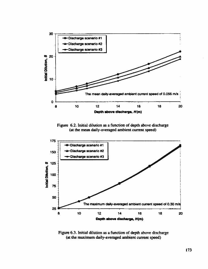
~~==============~---------------------; ._Discharge scenario 11
...-Discharge scenario 12
-Discharge scenario 13
V)2Q
i s a i = .5 10
' The mean daily-averaged ambient current speed of 0.056 mls !
0+. --------~--~--~------~--~----~--~--~------~ 8 10 12 14 16 18
Depth above di8Charge. H(m)
Figure 6.2. Initial dilution as a function of depth above discharge (at the mean daily-averaged ambient current speed)
20
175~================~-------------------------------------------------------------~ .,.Discharge scenario 11
150 ..-Discharge scenario 12
-Discharge scenario 13
V) 125 i ~ iS I
100
.s 75
50
i i ' i I
i I
The muimum daily-awraged ambient current speed of 0.30 mlsl I
25~------~------~-----------~--~--~------~--~--~· 8 10 12 14 16 18
Depth above dl..:harge, H(m)
Figure 6.3. Initial dilution as a function of depth above discharge (at the maximum daily-averaged ambient current speed)
20
173

15~--------------------------------------------------~ Discharge scenario 11:
I · •· · 8-m depth • o- ·1 O.m depth • •· 11-m depth
I · 6• ·14-m depth • • ·17-m depth • t> · 20.m depth
~ 10 -~ , Fash growth NOEC of 4.9%
I 5~---~~: •. :~·-·--~--~~--------------~~--~~~~~~~~ • • • b •••• • .. • .. Fish survivajl NOEC of 2.5% t. . ~ .... i.. .. ...... .
~:s ... '.~ ··::o._. ····•····•··· • . ·ii- : """ ii- : : : 4}.: - - =~ ~: : : :. : : : : ~: : : : ~: : : : ~: : : : ~: : : :~ ... ·c----·~-:.·.· .... 4:::: -··· ........... . ····C···· :::: :::: :::z :::a
0+. ------------~----------~------------~----------~ 0 50 100
aown.tr.m dlatance (m)
150 200
Figure 6.4. Centerline concentration as a function of distance downstream (relative density difference of 0.037)
15.---------------------------------------------------. . .
'
Discharge scenario 12:
• •· ·8-m depth • o· ·10.m depth • •· ·11.m depth
• 6· ·14-m dep1h • • ·17-m depth • o- · 20.m depth
# 10 -
I . ' ' . .
0
..... .. . .. ' . . .
Ash growth NOEC of 4.9o/o
50 100 150 200
Figure 6.5. Centerline concentration as a function of distance downstream (relative density difference of 0.025)
174

15~.~------------------------------------------------. •
- . . '# tO • • ....... " .. '
Discharge scenario •3:
I · •· ·8-m depth • o- ·1 ~m depth
I · -6· - t~m depth • • ·17-m depth
g • • • ::; '. '. • t=ish growth NOEC of 4.9%
• •· ·11-m depth
• o- ·20-m depth
I! ' ' • Ill Fish survival NOEC of 2.5%
o ~ , ',o. • • • • •• U-~~ .. ·, .......
5 ', .... o.. . ...... .. I .... ·.. .. • - " " • • ~ • .... • 0 • .. • • .. e .. .. • e • .... • e • ...... e
', '• ....• ::::o····o- ..... I ........... .,. •• A··· A •·········i-- ·O····O····t"l ~ Ullll • - ••••A •&••••&••••:J:
• .. _•····•.. - ·g••••.a.····A····A····A ~--··u-:::o--·-•···· ' ····u····O====O====O====O====e
0+---~~------~--------------~------------~---------~~ 0 50 100
Down.,_m dtmnce (m)
150 200
Figure 6.6. Centerline concentration as a function of distance downstream (relative density difference of0.013)
As discussed in section 2.3 (Chapter Two), sufficiently high initial dilutions are required to
maintain minimal thickness of the effluent slick. Unlike mixing in the far field, which is
mainly governed by ambient characteristics, initial dilution is highly dependent on the
design of the discharges. Despite its importance in design, however. no fixed threshold
value has been defined as an .. acceptable initial dilution". This might be because it likely
depends on the type of the discharges (e.g. sewage. cooling water, produced water etc.), the
quantity and quality of the discharge, and the environment where the discharge takes place.
For example, an ocean outfall discharging sewage from a small town in Newfoundland into
Spaniard's Bay was designed to achieve initial dilution of about 30 (Gowda 1992); while a
diffuser design for sewage discharge from a metropolitan city of Boston was b:~Sed on an
175

experiment, in which initial dilution was about 60 to 80 (Robens and Snyder 1993). For
produced water, Hodgins and Hodgins (2000) estimated that a potential produced water
discharge from the White Rose oil field, Grand Banks, Newfoundland, would have initial
dilution of 35.
The above calculations show that the range of dilution values associated with different
ambient current speeds for a given scenario is very wide. For instance, the initial dilution
for the discharge # 1 and scenario #6 (Table 6.5) ranges from 22.1 (at the mean current
speed) to 165.4 (at the maximum current speed), showing a more than 7-fold difference.
Initial dilution is also sensitive to the depth above discharge. The effect of the density
difference is less dominant than that of the ambient current speeds as presented in Figures
6.2 and 6.3. Those figures show that9 in this typical analysis, at the ambient current speed of
0.3 rnls the initial dilutions are practically the same irrespective of the variation in the
relative density difference. Because of this, the number of discharge scenarios associated
with the relative density difference may be reduced in the next analysis by considering the
minimum and maximum estimates, i.e. 0.013 and 0.037. Another treatment may also be
employed by taking the probability distribution of the relative density difference, instead of
using only its mean value of0.025.
Although the initial dilution is relatively low at the ambient cunent speed of 0.056 m/s, the
centerline concentrations are reduced very fast within 100 m downstream as shown in
Figures 6.4 to 6.6. When the relative density difference is high, i.e. 0.037 (Figure 6.4), at
100 m downstream all scenarios of depth above discharge result in centerline
176

concentrations below the fish growth NOEC of 4.9%. The majority of the scenarios (except
the 8-m depth) is associated with centerline concentrations below the fish survival NOEC
of 2.5%. In Figure 6.6, however, half of the scenarios are not in compliance with the
threshold concentration for fish survival at 100m downstream.
From the above analysis, it can be seen that the deeper the discharge pon, the better the
performance of the outfall in tenns of the initial dilutions and effluent concentrations
downstream. However, for the reason of construction, operation, maintenance and cost. an
extremely deep outfall may not be appropriate. If the distance of 100 m downstream is
assumed as the length of the mixing zone at which the effluent concentration should not
exceed the most stringent threshold value, i.e. the fish survival NOEC of 2.5%, scenarios
#l and #2 (the depth above discharge of 8 and 10 m) may then be screened off. The
scenario # 3 (the depth above discharge of 11 m) exceeds the threshold value only when the
relative density difference is low, i.e. 0.013 (Figure 6.6), but not in the other two cases.
Because of this, and because the above analysis is very conservative (i.e. effluent plume is
assumed always to be spreading towards the location of interest, no other direction is
considered), the scenario #3 (the depth above discharge of 11 m) will still be considered for
further analysis. On the other hand, the scenarios #5 and # 6 (the depth above discharge of
17 and 20 m) have almost the same value of the effluent concentrations at 100 m
downstream in all three cases, which are well below both the threshold concentrations.
Only one of them needs to be considered for further analysis. Therefore, scenarios #3, #4
and #5 (i.e. the depth above discharge of 11, 14 and 17 m) will be further evaluated as
discussed in the following steps.
177

6.4.4 Analysis of exposures and ecological effects
The analysis of exposure and ecological effects is based on the principles of
ecological risk assessment discussed in Chapter Five (Section 5.3.1 ). The analysis of
exposure considers the source of the pollutant, distribution of the contaminants, and modes
of contact between the pollutants and the endpoint biota. No other source of produced water
is identified near the Terra Nova project; the nearest is that from Hibernia (at about 35 km
distance). Further developments at White Rose (85 km away) and Hebron (20 km away) are
also beyond the distance of interest considered in the mixing zone analysis. It is therefore
assumed that the source is a single source of produced water outfall.
The U.S. EPA (1998) approach, which is discussed in Chapter Five (Section 5.3.2). is
adopted in the case study to estimate the exposure. In this approach, the exposure is
quantified using an environmental concentration of pollutant, assuming that the effluent is
well mixed in the ocean or that organisms move randomly through the water. Therefore,
distribution of effluent concentrations can be referred to as "exposure concentrations" (U.S.
EPA 1998). The exposure concentrations may be evaluated for each scenario under
consideration. The distribution of the exposure concentrations for the case study was
estimated based on hydrodynamic modeling discussed in the previous chapter (Chapter
Four). For the case study, the statistics of the concentrations are presented in Figures 6.7 to
6.12, showing the mean and the 95%-tile exposure concentrations at different scenarios of
depth above discharge (i.e. 11. 14 and 17 m) and relative density difference (i.e. 0.013 and
0.037). The 95%-tile exposure concentrations based on uniformly distributed relative
density difference (referred to as discharge #4) are also shown in Figures 6.13 to 6.15.
178
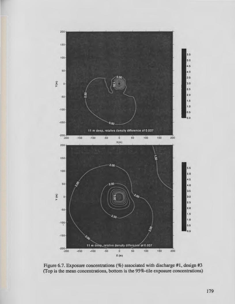
5.5
5.0
4 .5
4 .0
3 .5
E 3.0 >
2 .5
2 .0
1.5
1.0
0.5
0.0
5.5
5.0
4 .5
4 .0
3.5
.s 3.0 >
2 .5
2 .0
1.5
1.0
0.5
0.0
X (m)
Figure 6.7. Exposure concentrations(%) associated with discharge #1, design #3 (Top is the mean concentrations, bottom is the 95%-tile exposure concentrations)
179

5.5
5 .0
4 .5
4 .0
3 .5
.s 3.0 >
2.5
2 .0
1.5
1.0
0 .5
0 .0
5.5
5.0
4 .5
4 .0
3 .5
I 3 .0 >
2.5
2 .0
1.5
1 .0
0 .5
0.0
X (m)
Figure 6.8. Exposure concentrations(%) associated with discharge #1, design #4 (Top is the mean concentrations, bottom is the 95%-tile exposure concentrations)
180

5.5
5.0
4 .5
4 .0
3 .5
.§. 3.0 >-
2 .5
2 .0
1 .5
1.0
0 .5
0 .0
5.5
5.0
4 .5
4 .0
3.5
.§. 3.0 >-
2.5
2 .0
1 .5
1.0
0.5
0.0
X(m)
Figure 6.9. Exposure concentrations(%) associated with discharge #1, design #5 (Top is the mean concentrations, bottom is the 95%-tile exposure concentrations)
181

5 .5
5 .0
4 .5
4 .0
3.5
~ 3 .0 >-
2 .5
2 .0
1.5
1 .0
0 .5
0 .0
X(m)
5.5
5 .0
4 .5
4 .0
3 .5
~ 3 .0 >-
2 .5
2 .0
1.5
1 .0
0 .5
0 .0
X (m)
Figure 6.10. Exposure concentrations(%) associated with discharge #3, design #3 (Top is the mean concentrations, bottom is the 95%-tile exposure concentrations)
182

5.5
5 .0
4.5
4.0
3 .5
I 3.0 >
2 .5
2.0
1.5
1.0
0 .5
0 .0
5.5
5 .0
4.5
4.0
3.5
I 3.0 >
2 .5
2 .0
1.5
1.0
0 .5
0.0
X (m)
Figure 6.11. Exposure concentrations(%) associated with discharge #3, design #4 (Top is the mean concentrations, bottom is the 95%-tile exposure concentrations)
183

5.5
5 .0
4.5
4.0
3 .5
I 3.0 >-
2.5
2.0
1.5
1.0
0.5
0 .0
5 .5
5.0
4.5
4.0
3 .5
I 3.0 >-
2 .5
2.0
1.5
1.0
0 .5
0.0
X(m)
Figure 6.12. Exposure concentrations(%) associated with discharge #3, design #5 (Top is the mean concentrations, bottom is the 95%-tile exposure concentrations)
184

5.5
5.0
4 .5
4.0
3 .5
g 3.0 >-
2 .5
2 .0
1.5
1.0
0 .5
0.0
5.5
5.0
4 .5
4.0
3 .5
g 3.0 >-
2.5
2.0
1.5
1.0
0 .5
0 .0
X (m)
Figure 6.13. Exposure concentrations(%) associated with discharge #2, design #3 (Top is the mean concentrations, bottom is the 95%-tile exposure concentrations)
185

5.5
5 .0
4.5
4 .0
3 .5
I 3.0 >-
2 .5
2.0
1.5
1.0
0 .5
0 .0
5 .5
5.0
4.5
4 .0
3 .5
I 3.0 >-
2.5
2.0
1.5
1.0
0 .5
0 .0
X (m)
Figure 6.14. Exposure concentrations(%) associated with discharge #2, design #4 (Top is the mean concentrations, bottom is the 95%-tile exposure concentrations)
186
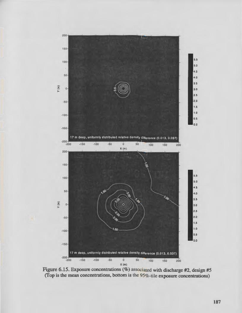
5.5
5.0
4.5
4.0
3.5
I 3.0 >-
2.5
2 .0
1.5
1.0
0 .5
0 .0
5 .5
5.0
4.5
4.0
3 .5
I 3.0 >-
2 .5
2.0
1.5
1.0
0.5
0.0
X (m)
Figure 6.15. Exposure concentrations(%) associated with discharge #2, design #5 (Top is the mean concentrations, bottom is the 95%-tile exposure concentrations)
187
It can be seen from Figures 6.7 to 6.15 that the effect of the depth above discharge to
exposure concentrations is generally significant. For example. for the relative density
difference of 0.037, the area of the mean exposure concentrations of 0.5% or more typically
reduces from approximately 17,000 m2 (Figure 6. 7. top: 11 m depth) to approximately
1,900 m2 (Figure 6.9, top: 17m depth), or about 88% in reduction. Similar evidence is also
observed for the area of the mean exposure concentrations of 0.5% or more at the relative
density difference of 0.013 (Figures 6.10 to 6.12. top). and for the area of the 95%-tile
exposure concentratior.s at the relative density difference of0.013 and 0.037 (Figures 6.7 to
6.12. bottom).
The effect of the density difference is also observed from those figures but in general is
relatively less than that from the depth above discharge. From the previous section, it
appears that the effect of the relative density 'Jifference on the exposure concentrations is
!ess dominant than that of the ambient current speeds (shown in Figures 6.2 and 6.3).
Unlike the depth above discharge. which is a design scenario and is specified upon the
decision of the designer. the relative density difference is a discharge characteristic
depending on the physical characteristics of produced water, which are not controllable. In
addition, only a range was available for the estimates of the relative density difference and
there was no evidence to support whether one value has more likelihood than another does.
For these reasons, uniform distribution may be a reasonable assumption to represent both
cases, the lowest and highest estimates of the relative density difference. Therefore, the
following risk characterization considers that the relative density difference is uniformly
distributed.
188

Once exposure concentrations have been define~ they may be integrated with the analysis
of ecological effects to enable characterization of ecological risks. The analysis of
ecological effects determines the relationships between the exposure to the contaminant and
effects on the measurement endpoint, and it is usually based on results of toxicity studies as
discussed in section 5.3.2 (Chapter Five). Ecological effects of produced water at the
organism level have been reponed in the literature. e.g. Brown et al. ( 1992), Meinhold et al.
(1996b, 1996c) and U.S EPA (1996b). Although field tests may be possible, most toxicity
tests of individual organisms are performed in the laboratory. Results of toxicity tests of
individual animals can be used as the basis for the effects assessment (Meinhold et al.
l996c). Acute and chronic effects are usually reponed in terms of the 96-hours median
lethal concentration LC50 and the Slm'ival or growth NOEC. respectively. Table 6.6 shows
typical results from toxicity studies of produced water on two organisms, i.e. Sheephead
minnows (fish) and Mysid shrimps (aquatic invertebrate).
Table 6.6. Typical results from whole effluent toxicity tests (after Meinhold et al.l996b)
Mysids Sheepshead Minnows
Statistics (Mvsidopsis bahia ) ( Cyprinodon varie atus)
96-hour 7-dNOEC 7-dNOEC 96-hour 7-dNOEC 7-dNOEC . . . LCso Survival Growth LCso Survival Growth
Mean 9.5 2.9 4.0 24.4 7.1 9.0
Standard deviation 11 2.9 3.5 38.2 5.1 6.9
Minimum 0.2 0.0004 0.1 2.4 0.2 0.2
Maximum 71.2 11.4 12.1 - 19.1 25.2
No. of outfaUs 41 43 42 39 41 39
189

As can be seen from Table 6.6, the aquatic organisms respond differently at various levels
of produced water concentration. As discussed in the problem formulation, the survival and
growth NOEC for both Sheephead minnows and Mysid shrimps are considered as
measurement endpoints. However. since the survival NOECs are more sensitive measures
than the growth NOECs (see Table 6.6), the use of survival NOECs as measurement
endpoints can reflect the protection level of both survival and growth NOECs for these
organisms.
Other ecological entities. which may also have adverse responses to produced water, may
also be considered. Aquatic ecological entities in the area under consideration are various.
which may be reflected by feeding relationships among species as shown in Table 6. 7. For
produced water as a whole effluent. repons of toxicity effects on various aquatic organisms
are not readily available. However, they may be evaluated in terms of chemical specifics
usually found in produced waters. As discussed previously, various chemicals reponed in
produced waters worldwide are shown in Tables 5.2 and 5.3 (Chapter Five). For the Terra
Nova project, studies have considered hydrocarbon chemicals (i.e. P AH) during the
evaluation of produced water effects in the environmental impact statement (Petro-Canada
1996). This analysis will therefore focus on other specific chemicals, i.e. a metal and a
radioactive chemical.
190
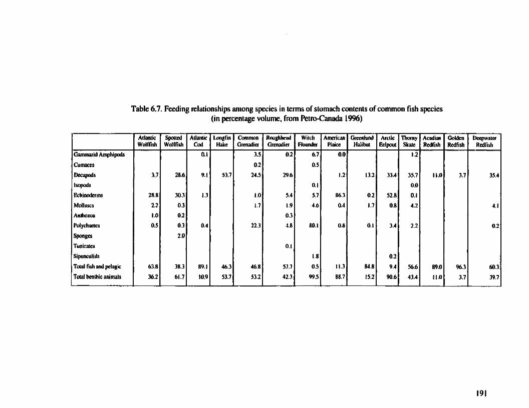
Oammarid Amphipods
Cumacea
Decapods
lsopods
Echinoderms
Molluscs
Anlhowa
Polychaeaes
Sponges
Tunicares
Slpunculids
Total fish IUld pelagic
Tocal benlhic animals
Table 6. 7. Feeding relationships among species in tenns of stomach contents of common fish species (in percentage volume. from Petro-Canada 1996)
Atlanaic Spoucd Atlantic Longtin Common Rooghhcad Witch American Grcentand Arctic Thorny Acadian Wolffish Wolffish Cod Hake Grcnadirr Grenadier Flounder Plaice Hali11111 Eel pour Skare Redfish
0.1 3.5 0.2 6.7 0.0 1.2
0.2 0.5
3.7 28.6 9.1 53.7 24.5 29.6 1.2 13.2 33.4 35.7 11.0
0.1 0.0
28.8 30.3 1.3 1.0 5.4 5.1 86.3 0.2 52.8 0.1
2.2 0.3 1.7 1.9 4.6 0.4 1.7 0.8 4.2
1.0 0.2 0.3
0.5 0.3 0.4 22.3 .u 80.1 0.8 0.1 3.4 2.2
2.0
0.1
1.8 0.2
63.8 38.3 89.1 46.3 46.8 57.1 o.s 11.3 84.8 9.4 56.6 89.0
36.2 61.7 10.9 53.7 53.2 42.3 99.5 88.7 15.2 90.6 43.4 11.0
Golden Deepwarrr Red fish Red fish
3.7 35.4
4.1
0.2
96.3 60.3
3.7 39.7
191

A detailed review of ecological effects of petroleum hydrocarbons, metals, and radioactive
materials has been reponed in Neff ( 1997). For metals, Neff ( 1997) noted that Barium (Ba),
Cadmium (Cd), Lead (Pb) and Zinc (Zn) typically have the highest enrichment factor (i.e.
the ratio of concentration in produced water and that in solution in seawater of
approximately on the order of 1000). In the context of ocean discharge of produced waters,
the review showed that Cd is generally the most potentially hazardous to the environment,
compared with the other three chemicals. Dissolved, ionic Cd is bioavailable and highly
toxic to marine organisms: even relatively low concentrations in sediments are considered
toxic (Neff 1997). Table 6.8 summarizes available toxicity information of Cd for different
species. Figure 6.16 presents the toxicity data from Table 6.8 in a form that is suitable for
assessing effects on the ecological community of interest. This figure employs a plotting
position approach so that the data can be assumed as a probability distribution of species
responses consistent with a methodology presented by Lenwood et al. (1998) and the U.S.
EPA (1998).
Other specific chemicals associated with produced water, which have not been assessed in
detail in the Terra Nova environmental impact statement for their potential ecological
effects, are radioactive materials {radionuclides). Radionuclides are known to occur in
produced water with typically very high enrichment, which can be up to about 6000 (Neff
1997). In addition to other decay products, ~a. 228Ra and 210pb may be expected in
produced water at relatively high concentration compared with other radioactive materials
(Meinhold et al. 1996b, Neff 1997).
192

100%
.~ ~ '5. u 1.11 ::s ... ~ ·~ ·;:c ~ ... u ·:; 8. ... ._ 0 ~ c ~
1:111:
90%
80%
70%
60%
SO%
40%
30%
20%
10%
0%
10 100
Concentration (Jig/l)
1000 10000
Figure 6.16. Planing position for the toxicity data summarized in Table 6.8 below
Code
A B c 0 E F
G H I
J K L
M
N
0 F Q
Table 6.8. A summary of available data on ecological effects of Cd on different species (adapted from Kennish 1997, Middleditch 1984)
Sublethal effects on various organisrm Concenttation (!'g/1)
Copepod reduction reduced 10
Decapod larval developftnt retarded so Enchinodenns (amsted fertilization and devclopftnt of sea urchin eggs) 600
Fish (reduced fcnilizalion of Spring-spawning hlning ) s Fish (reduced growth of P1~11ron~ct~s plat~ssa) s Fish hatch rare dec:reascd 2000
Hydroid growth rare reduced 28 Hydroids (ahered hydnnlh aaphology of Eir~n~ viridula) 10
Hydroids (reduced growth of Campanul4rilljlexll0sa) 195
Phytoplankton (reduced 1 .. C tixalion) I
Phytoplankton (reduced growth) 112
Polychaete reproduction suppressed 560
PolydWcs (reductions in reprodu&:tion of Capii~Ha capitllla) 560
Polychatcs (redu;tions in ~n of Ctenodrilus s~mmu) 2500 Polyc:hales (reductions in reproduction of N~anthls annac~tHkntata ) 1000
54:-.Uiop sruwlh ralc rcd..:al 78 Sbrimp gills blxkeued 760
193

Radioactivity has been quantified in tenns of the number of spontaneous energy emitting
transformations per unit time - a quantity . known as activity. An example of a
transformation is the decay of a radium 226 nucleus into a radon 222 nucleus, an alpha
particle and gamma ray. The unit of activity has historically been the Curie (Ci), in which
one Ci is equal to 3.7 x 10¹⁰ disintegrations per second. In the SI system, the unit has been
redefined as one disintegration per second, known as the Becquerel (Bq). One Curie is then
equal to 3.7 x 10¹⁰ Bq.
Exposure to ionizing radiation can result in injury at the molecular, cellular and whole body
level (Meinhold et al. 1996c ). The exposure to radionuclides is related to the absorbed dose
and dose rate. The absorbed dose is a measure of the energy impaned to matter and has the
Sl unit of the Gray (Gy, l Joule/kg). The ecological effects depend not only on the
absorbed dose but also the type and energy of radiation. Radiation weighting factors are
used to account for the differences in biological effectiveness of different radiation, such as
gamma and alpha panicles. The absorbed dose modified by the weighting factor is referred
to as the equivalent dose expressed in units of Joule/kg or Sieven (Sv). Meinhold et al.
(1996b, 1996c) have reviewed that thresholds of effects on aquatic biota are expected at the
equivalent dose of 0.004, l, and 10 mSv/hr for no adverse effects, reduced reproductive
success, and increased mortality threshold, respectively. Based on the International Atomic
Energy Agency (IAEA) dose conversion factors for typical fish species in 22~a
contaminated water (Meinhold et al. l996c), these doses are associated with radium
concentration in the water of 0.783, 195.65, and 1956.52 pCi/1 for no adverse effects,
reduced reproductive success, and increased mortality threshold, respectively.
194

6.4.5 Charaeterizing ecologkal risks
Characterization of ecological risks is based on the integration of the analysis of
exposures and ecological effects. The methods for characterizing ecological risks have been
discussed in Chapter Five (Section 5.3.3) and include qualitative and quantitative methods.
For the purpose of evaluating different design scenarios, the quantitative methods were
employed in this case study in a number of ways, including ( 1) the hazard quotients based
on the chronic benchmark concentrations of the whole effluent toxicity to individual
species, (2) the exceedance probability of the critical hazard quotient based on the whole
effluent toxicity approach, (3) the hazard quotients based on the no effect radium
concentration (chemical specific approach), (4) the exceedance probability of the no
ecological effect threshold of the chemical specific (radium), (5) and the protection level in
terms of percentage of ecological species affected as well as associated probability, based
on the chemical specific (cadmium) toxicity approach. For each of the above-mentioned
analyses, probability distributions of the parameters in the hydrodynamic models, i.e.
model inputs and coefficients, were taken from Table 4.2. As discussed in the previous
section, the discharge scenario #2, uniformly distributed relative density difference was
considered
For the case study at hand, the first characterization of risks was performed by evaluating
hazard quotients (HQs) associated with each design scenario. The characterization was
based on the chronic benchmark concentration of the whole effluent toxicity to individual
fish and shrimp species. From the analysis of ecological effects, measurement endpoints of
the survival NOECs for fish (Sheephead minnows) and shrimp (Mysids) were considered in
195

the analysis. From Table 6.6, the mean and standard deviation of the survival NOEC are
7.1% and 5.7%, respectively, for fish, and 2.9% and 2.9%, respectively, for shrimp. The
analysis presented in Chapter Five shows that the toxicity data (Mysid LCso) was
lognonnally distributed. Neither raw data on the NOECs nor their probability distributions
were available in this study; it was therefore assumed that the survival NOECs were also
lognonnally distributed. Using these inputs, MC simulations were performed and results of
the HQs associated with each design scenario are shown in Figures 6.17 to 6.22.
Hazard quotients (HQs) presented in Figures 6.17 to 6.22 can be viewed as "severity
measures" of risks as they show how far the exposure concentrations from the specified
benchmark concentrations are. When the hazard quotient is more than unity, ecological
effects, e.g. fish growth, may be expected. The higher the value of HQ above unity, the
more the ecological risks expected. Since uncertainty is taken into account in the analysis,
each HQ for a specified point near the discharge location is also uncertain and those figures
show the statistics of the HQ in tenns of 95% and 99%-tiles.
To evaluate the probability that ecological risks may be expected, probabilistic analysis was
performed to calculate the exceedance probability of HQs more than unity. An exceedance
probability is the probability of the exposure concentrations exceeding the chronic
benchmark concentrations of the whole effluent toxicity to individual fish and shrimp
species. For the case study at han~ exceedance probabilities associated with each design
scenario are presented in Figures 6.23 to 6.28.
196

3.6
3.2
2.8
2.4
I 2 .0 >
1.6
1.2
0.8
0.4
0.0
3.6
3.2
2.8
2.4
I 2.0 >
1.6
1.2
0.8
0.4
0.0
X (m)
Figure 6.17. Whole effluent chronic hazard quotients, design #3 (Fish survival risks: top is 95%-tile HQ and bottom is 99%-tile HQ)
197

3.6
3.2
2.8
2.4
~ 2.0 >
1.6
1.2
0.8
0.4
0.0
X (m)
3.6
3.2
2 .8
2 .4
~ 2.0 >
1.6
1.2
0.8
0.4
0.0
X(m)
Figure 6.18. Whole effluent chronic hazard quotients, design #3 (Shrimp survival risks: top is 95%-tile HQ and bottom is 99%-tile HQ)
198

3 .6
3.2
2.8
2.4
I 2 .0 >-
1.6
1.2
0 .8
0.4
0.0
3.6
3 .2
2 .8
2 .4
I 2.0 >-
1.6
1.2
0.8
0 .4
0 .0
X(m)
Figure 6.19. Whole effluent chronic hazard quotients, design #4 (Fish survival risks: top is 95%-tile HQ and bottom is 99%-tile HQ)
199

3.6
3.2
2 .8
2.4
:§: 2.0 >
1.6
1.2
0.8
0.4
0.0
X (m)
3.6
3.2
2.8
2.4
:§: 2 .0 >
1.6
1.2
0.8
0.4
0.0
X (m)
Figure 6.20. Whole effluent chronic hazard quotients, design #4 (Shrimp survival risks: top is 95%-tile HQ and bottom is 99%-tile HQ)
200

3.6
3.2
2.8
2 .4
~ 2 .0 >
1.6
1.2
0.8
0.4
0 .0
3.6
3.2
2 .8
2 .4
~ 2 .0 >
1 .6
1.2
0.8
0.4
0.0
X (m )
Figure 6.21. Whole effluent chronic hazard quotients, design #5 (Fish survival risks: top is 95%-tile HQ and bottom is 99%-tile HQ)
201

3.6
3.2
2 .8
2.4
§: 2 .0 >
1.6
1 .2
0.8
0 .4
0.0
X (m)
3.6
3.2
2 .8
2 .4
§: 2.0 >
1.6
1.2
0.8
0.4
0 .0
X (m)
Figure 6.22. Whole effluent chronic hazard quotients, design #5 (Shrimp survival risks: top is 95%-tile HQ and bottom is 99%-tile HQ)
202

10
8
6
3
2
0
y (m)
Figure 6.23. Exceedance probability (%) of the whole effluent chronic benchmark (Fish survival risks, design# 3)
.E. >-
"
~ ------~~ ~0 '--, " ·,
'0 "\"., ·o \
\ I )
\ ~
, I
.Exceedance probability(%), shrimp survival benchmark , deep1~ utfal l 0
X (m)
10
9
8
7
6
5
4
3
2
0
Figure 6.24. Exceedance probability (%) of the whole effluent chronic benchmark (Shrimps survival risks, design# 3)
203
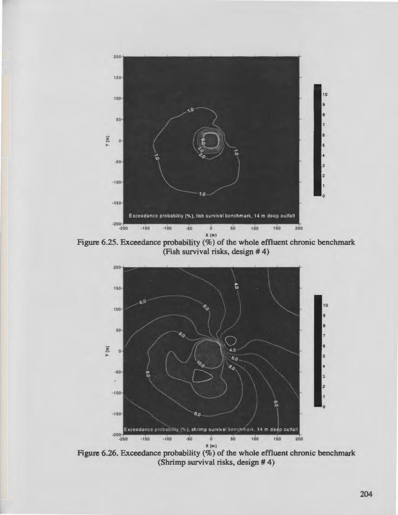
10
9
8
7
6
5
4
3
2
0
X(m)
Figure 6.25. Exceedance probability(%) of the whole effluent chronic benchmark (Fish survival risks, design# 4)
10
9
8
7
:§: 6
> 5
4
3
2
0
/ .o. I "o I i ·0 I e.o
CJ> \ ( -- . ' 0 I '---
\ \ '-........ ~l--
_.) \ \
' ' -~ \~ _ __/ ~" / .,..
•, -~ / ·o
B.o -----~-___./'
/ Exceedance probability (',o), shr1mp surv1val benchmark. 14m deep outfall
X(m)
Figure 6.26. Exceedance probability (%) of the whole effluent chronic benchmark (Shrimp survival risks, design# 4)
204

10
9
8
7
6
5
4
3
2
0
X (m)
Figure 6.27. Exceedance probability (%) of the whole effluent chronic benchmark (Fish survival risks, design# 5)
10
9
8
7
6
4
3
2
0
X (m)
Figure 6.28. Exceedance probability (%) of the whole effluent chronic benchmark (Shrimp survival risks, design # 5)
205

In the previous approaches of risk characterization. the whole effluent toxicity data were
employed by using the chronic fish and shrimp survival NOECs. Ecological risks may also
be assessed from chemical specific basis. In the previous subsection. the analysis of
ecological effects has identified two specific chemicals, namely radium (22~a) and
cadmium (Cd). In this third approach of risk characterization, the hazard quotients (HQs)
associated with 22~a were evaluated by using the ratio of the exposure concentrations to
the 2~a benchmark concentration. As discussed in the analysis of ecological effects. the
22~a threshold concentrations for bathypelagic fish are 0.78, 195.65. and 1956.52 pCi/1 for
no adverse effects, reduced reproductive success, and increased mortality threshold,
respectively.
No estimate of radium concentration is available for the Terra Nova project. If radium
concentrations from other oil fields are used as estimates. 22~a concentration may be
assumed to be in the range of 4 to 584 pCill. with the average of 262 pCill. based on
produced water from 42 oil production platfonns from the Gulf of Mexico (shown in Table
5.2, Chapter Five). With this limited infonnation, radium concentration may be typically
assumed to follow a triangular distribution, with a range from 4 to 584 pCi/1 and the most
likely value of 262 pCi/1. From these 22~a concentrations, no fish monality risk may be
expected. Results of the MC simulations showed that risks to the fish reproductive success
were also negligible since, for example, the maximum concentration at the water surface
above discharge point, 0(0,0), for the design #3 ( 11 m deep outfall) is typically about 98
pCi/1 or only about half of the reproductive success threshold. If. however. no adverse
effect threshold was adopted. potential effects were noticed {Figures 6.29 to 6.34).
206

15
14
12
11
9 E. > 8
6
5
3
2
0
15
14
12
11
9 E. > 8
6
3
2
0
-200 -150 -100 -50 0 50 100 150 200
X (m)
6.29. Chemical specific, 22~a hazard quotients, design #3. (Risks on fish: top is the 95%-tile HQs and bottom is 99%-tile HQs)
207

15
14
12
11
9
8
6
5
3
2
0
X(m)
15
14
12
11
g >- 8
6
5
2
0
X (m)
6.30. Chemical specific, 226Ra hazard quotients, design #4. (Risks on fish: top is the 95%-tile HQs and bottom is 99%-tile HQs)
208

15
14
12
11
9
8
6
3
2
0
15
14
12
11
8
6
3
0
X (m)
6.31. Chemical specific, 22~a hazard quotients, design #5 (Risks on fish: top is the 95%-tile HQs and bottom is 99%-tile HQs)
209

50
45
40
35
30
25
20
15
10
0
X(m)
Figure 6.32. Exceedance probability (%) of the 22~a benchmark, design #3
50
45
40
35
30
25
20
15
10
5
0
X (m)
Figure 6.33. Exceedance probability(%) of the 226Ra benchmark, design #4
210

X (m)
Figure 6.34. Exceedance probability (%) of the 226Ra benchmark, design #5
In the last approach of risk characterization, the protection level in terms of the percentage
of ecological species affected as well as associated probability are evaluated for each design
scenario. The evaluation is based on data of the chemical specific toxicity data in Table 6.8
presented in the previous subsection. Information on estimates of cadmium concentration
for the Terra Nova project is not available for this study. If it is assumed that cadmium
concentrations reported from the North Sea based on six discharges from offshore
platforms (Table 5.2, Chapter Five) can be used as estimates for the case study, cadmium
concentrations may be assumed to follow a triangular distribution with a range from 20 to
10,000 J.Lg/1 with the most likely value of 6670 J.Lg/1. As a metal, cadmium may leach so that
the concentration in the water column may be expected to be lower than that calculated
211

based on the total concentration. To take leaching into account, a leach factor of 0.11 (U.S.
EPA 1999b) was used in this analysis.
To illustrate the procedure of evaluating the protection level, consider a typical point A
located at a 100 m radius from the origin 0(0.0) as shown in Figure 6.35 (top). For this
particular point. exposure concentrations associated with each design scenario can be
obtained from MC simulations. Then, the exposure concentrations are presented in tenns of
a cumulative distribution and are superimposed with the toxicity data associated with
cadmium (Figure 6.16, the previous subsection). A typical presentation for evaluating the
protection level at the point A is shown in Figure 6.35 (bottom). From Figure 6.35
(bottom), it can be seen that, for example, scenarios #3, #4, and #5 can be associated with
the protection from the violation of the 95% of the species toxicity thresholds for 69.8%,
75.5%, and 79.8% probability, respectively. This means that there is an exceedence
probability of 30.2%, 24.5%, and 20.2%, respectively.
The procedure presented here is similar to that from Lenwood et al. (1998) and the U.S.
EPA {1998). In this case study, the protection level for each point of interest near the
discharge was considered and a probability field exceeding a specified protection level was
drawn based on results of the MC simulations. If, for example, protection of 95% of the
species toxicity thresholds is of concern, the exceedance probability field for whole region
of interest can be estimated as shown in Figures 6.36 to 6.38.
212

200
ISO 100 mradius
100
so
-!. 0 >
-SO
-100
-ISO
-200 +--~-....,.....-~----r----~-...-----
-200 -ISO -100 -SO 0 so 100 150 200
X(m)
100% 100%
9Q0_4 90%
80% 80% ?: ~
c: 70% 700/o i .2 ~ :I
60% 60o/o en c: ~ ~ 50% 50% )C c u -, t 0 40% 40%
u... c ~Cd diStribution. 11 m deep outfal 0 30% 30%
-a-Cd diltrib&aion, 14 m deep oUifal 0 20% -a-Cd distribution, 17 m deep outtau 20% '! ca
~
10% ~ ToJUc:ity data on various species 10o/o
0% 0% 1 10 100 1000 10000
Concentration (~gil)
Figure 6.35. Cadmium protection level (the 95% aquatic species toxicity thn~sholds) and associated probability: Location of a spot A (top) and the protection level (bottom)
213

50
45
40
35
30
25
20
15
10
0
0
X (m)
Figure 6.36. Exceedance probability (%) of the Cd protection level, design #3
50
45
40
35
30
25
20
15
10
0
X (m)
Figure 6.37. Exceedance probability (%) of the Cd protection level, design #4
214

X(m)
Figure 6.38. Exceedance probability (%) of the Cd protection level, design #5
As discussed, characterization of ecological risks was performed in various ways and the
results were shown in Figures 6.17 to 6.38. From these figures, in general, the choice of the
design scenario directly affects the extent of the potential ecological risks associated with
the produced water discharge. This makes it possible to provide design recommendations
on the basis of ecological risks. More detailed discussion of effects of the design scenarios
on the potential ecological risks is presented in the next subsection.
It should be noted here that ecological risks associated with each design scenario described
above are subject to uncertainty. Uncertainty associated with hydrodynamic modeling has
been quantitatively taken into account as discussed in Chapter Four. Another uncertainty is
215

associated with assumption used in the modeling. The assumption needs to be considered
with care so that they are reasonably suitable for the case under investigation. The case
study used several assumptions that directly affect the results of the characterized
ecological risks as presented in Figures 6.17 to 6.38 above. These assumptions include the
flow rate of the produced water discharge, Cd and ~a concentrations in the produced
water prior to discharge. relative difference of the produced water and ambient water
densities, and the toxicity benchmarks such as fish and shrimp survival benchmark
concentrations, 22~a no adverse effects concentration, and Cd protection level. Use of the
results of the analysis may not be possible until these assumptions are accepted.
6.4.6 Discussion and design recommendations
As discussed previously, the problem in an ecological risk-based design it to find
design scenarios that may be associated with the least ecological risks. The problem
formulation has determined that fish and shrimp survival NOECs may be used as
measurement endpoints in the characterization of ecological risks. The potential fish and
shrimp risks were evaluated based on the whole effluent toxicity approach. For comparative
and discussion purposes, other potential ecological risks were also evaluated to look at
potential effects of the radium and the cadmium protection level.
It appears from the risk characterization above that the extent of the ecological effects may
be reduced by selecting an appropriate design scenario. In general, the deeper the water
above discharge, the less the area potentially associated with ecological effects. For fish,
although design lt5 is associated with the least survival risks among other designs, HQs for
216

all design scenarios are generally low except in the area very close to the discharge point
For example, Figures 6.17, 6.19 and 6.21 show that the 95%-tile fish survival HQs
exceeding unity are observed only in the area less than 500m2 (about 40 min radius). Even
the 99%-tile fish survival HQs are reasonably low and are within a typical regulatory
mixing zone of radius of about 400 m (Huang et al. 1996). Exceedance probabilities for the
fish survival benchmark presented in Figures 6.23, 6.25 and 6.27 reveal the same results.
For shrimp. survival risks are expected to be higher than those for fish because benchmark
concentrations for shrimp are lower than those for fish (Table 6.6). These are observed in
Figures 6.17 to 6.28 above. Shrimp survival HQs are generally low, particularly those
associated with designs #4 and #5. For all design scenarios, the 95%-tile shrimp survival
HQs of 2 are within an area of approximately within 31,500 m2 (about 100m in radius) as
shown in Figures 6.18, 6.20 and 6.22. For design #3, the 99%-tile HQs seem to be higher
(Figure 6.18) and the exceedance probabilities of 10% are within an area with a radius of
about 175m (Figure 6.24). In design #5, the exceedance probability of 5% is within an area
of about 70,000 m2•
Considering the .. measurement endpoints defined in the problem formulation, the
acceptability of the design scenarios may be evaluated from Figures 6.17 to 6.28 above.
However, the acceptability has also to be evaluated based on an allowable area of specified
ecological effects and associated exceedance probability. Traditionally, criteria associated
with wastewater discharges have been defined by legislation which, in many jurisdictions,
leans towards the mixing zone concepts. For example. a maximum allowable surface area
217
of 502,655 m2 (or equivalent circular area with a radius of approximately 400 m) was
defined as a mixing zone in the state of Florida, U.S.A. (Huang et al. 1996). The state of
Michigan determined a mixing zone with a radius of approximately 300 m (Doneker and
Jirka 1990). On the other hand, engineering design of an ocean outfall is currently not
explicitly based on ecological risk criteria (although they could be in the future), which are
an acceptable way of comparing one outfall to a number of alternatives from the ecological
point of view. For example, if an exceedance probability of 10% for fish and shrimp
survival HQs at a maximum mixing zone of 150m in radius are specified as the criteria,
then design #4 is acceptably good. The challenge is now to define the criteria for different
purposes of ecological protection in different environments. This may be recommended as a
potential new research direction and is beyond the scope of this study.
As indicated, design recommendations depend on the ecological protection, which is
reflected by use of measurement endpoints as discussed in the problem formulation. For
comparative purposes, the risk characterization was also performed using measurement
endpoints other than those defined in the problem formulation. These were based on the
chemical specific approach, i.e. the 22~a no adverse ecological effect and Cd protection
level. As discussed. no fish mortality risk associated with ~a may be expected in this
case study. and risks to the fish reproductive success were also negligible. However. if the
~a no adverse ecological effect was defined as the measurement endpoint. Figures 6.29
to 6.34 show that none of the design scenarios are acceptable based on the exceedance
probability of 10% at a maximum mixing zone of 150 m in radius in the above example. In
this case. the design may be modified by, for example, adopting a diffuser type of outfall.
218

The following case shows another example how recommendations may be given using the
Cd protection level based on available toxicity data. If the protection of 95% of the species
toxicity thresholds is of concern. it appears from Figures 6.36 to 6.38 that the exceedance
probability of the specified protection level may typically be considered to be high and no
design scenario satisfies the exceedance probability of 10% at a maximum mixing zone of
150 m in radius in the above example.
As shown in Figure 6.35, the protection level in this typical analysis was associated with a
threshold Cd concentration of about 4 J.Lg/1, at which only the toxicity benchmark of J
(reduced 14C fixation of phytoplankton) is exceeded (Table 6.8). MC simulations were also
carried out to evaluate the exceedance probability when the protection level was lowered to
the 90% toxicity benchmarks. At this protection level, the toxicity benchmarks of 0, E and
J (reduced fertilization of Spring-spawning herring, reduced growth of Pleuronectes
platessa, and reduced 14C fixation of phytoplankton) are allowed to be exceeded. With this
change, the exceedance probability for designs #3 and #5 are shown in Figure 6.39 and 6.40
below. It can be seen that at this protection level design #5 is acceptable to satisfy the
exceedance probability of 10% at a mixing zone of 150m in radius in the above example.
219
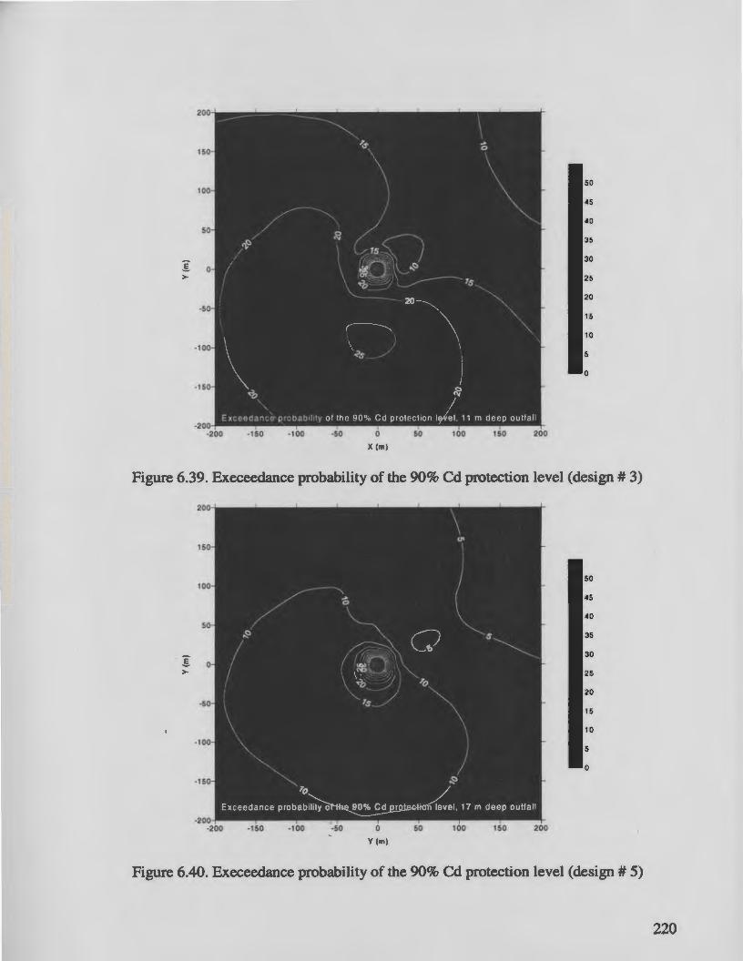
50
45
40
35
30
25
20
15
10
5
0
X (m)
Figure 6.39. Execeedance probability of the 90% Cd protection level (design# 3)
50
45
40
35
30
25
20
15
10
5
0
Y (m)
Figure 6.40. Execeedance probability of the 90% Cd protection level (design# 5)
220

6.5. Summary
A framework for the design on the basis of potential ecological risks is presented in this
chapter. The relevance of the framework is highlighted by reviewing traditional outfall
design approaches, which are conventionally directed at compliance with relevant water
quality standards. The standards are in tum commonly specified upon an epidemiological
and ecological viewpoint. As a complementary tool, the framework suggests a possibility
that the design of produced water outfalls could itself be looked at from the point of view of
the environmental risk from exposure to produced water or specific pollutants associated
with the produced water.
The framework of ecological risk-based design is developed by integrating the
methodology of hydrodynamic modeling and ecological risk assessment, which has been
discussed in Chapters Four and Five. The framework is directed at providing design
recommendations on the basis of ecological risk perspectives. The framework is
straightforward and consisted of six steps, and is discussed systematically within this
chapter by evaluating scenarios of produced water discharge relevant to an offshore oil
production platfonn located on the Grand Banks, southeast of St. John's, Newfoundland.
Canada. Instead of providing a solution for a particular problem of an existing oil
production platfonn, the emphasis of the case study is to show how the risk-based design of
produced water discharge could be undertaken.
221

Chapter 7
Conclusions and Recommendations
7 .1. Conclusions
In this section, conclusions are presented in the context of the scope and purpose of the
research, in which the general objective was to develop a methodology for ecological risk
based design of produced water discharge from an offshore oil production platform. The
study was carried out through integrating a probabilistic hydrodynamic model with an
ecological risk assessment model, and consisted of six parts: (1) developing an initial
dilution model; (2) integrating the developed initial dilution model with far field dilution
models; (3) developing a methodology for probabilistic hydrodynamic modeling; (4)
identifying methodologies for ERA of produced water discharge; (5) developing a
framework for ecological risk-based design of produced water outfall; and (6) applying the
framework for a case study dealing with an outfall design of potential discharge from an oil
offshore platform.
222
Keeping in perspective these objectives, it can be concluded that:
l. An initial dilution model was developed after conducting a critical review of presently
used initial dilution models, with emphasis on their conceptual and numerical problems
as discussed in Chapter Two. A new model is proposed in Chapter Three as an
alternative initial dilution model, which is more elegant and more justifiable. The model
was derived based on the hypothesis of additive shear and forced entrainment combined
with nonlinear regression. It gives a unique, continuous, solution of centerline dilution,
which can be presented in either a deterministic or probabilistic form. Comparison of
the proposed model with other available models shows that the proposed model is better
in a number of ways: (1) it does not assume that the current has no effect in the BDNF,
which asymptotic solutions do; (2) in the BDFF region the model has one parameter
fewer than the Huang et al. (1998) model yet it is no less accurate; (3) in the transition
region it gives a unique solution which the asymptotic models do not; (4) unlike the
Huang et al. (1998) model, the proposed model has approximately the same precision
for all regions, i.e. the BDNF, the BDFF, and the transition; and (5) the proposed model
can also be presented in a probabilistic form that permits calculation of fai ·~ ure
probability for specified model inputs and a threshold dilution.
2. An integrated hydrodynamic model is presented in Chapter Four. A mixing process
occurring in two separate regions, near and far fields, were discussed and integrated.
Modeling of the intennediate region connecting the near- and far-fields was provided
using a control volume approach. An application example of the integrated model was
discussed using a comparison with a presently available model. i.e. the CORMIX
223

model. The comparison showed that the proposed model and the CORMIX model are
generally in good agreement, particularly in estimating average effluent concentrations.
However, the proposed model also provides a concentration field in the X-Y directions
so that it may be applicable for analysis of the mixing zone, which in some cases is
defined in terms of horizontal area around the discharge location. The proposed model
is also readily modified into a probabilistic analysis to take into account uncertainty
associated with model inputs and model coefficients.
3. A methodology for probabilistic analysis was developed in Chapter Four for
hydrodynamic modeling using Monte Carlo (MC) simulations. Concern regarding the
··excessive,. number of simulations was addressed by comparing two methods of
sampling in the simulations, i.e. random sampling and Latin Hypercube Sampling
(LHS) methods. A comparison between random sampling and LHS for MC simulations
of a case of hydrodynamic modeling shows that LHS-based MC simulations are
typically about 15% more efficient that the random sampling MS simulations. This
chapter also shows that probabilistic analysis not only provides distribution shapes. but
also takes into account the uncertainty factors simultaneously.
4. In Chapter Five, methodologies for ERA of produced water discharge were presented
and problems associated with presently used approaches were discussed. Substantial
effort has been devoted in the past to assessing ecological risks of produced water
discharges; however, ERA was usually directed at monitoring purposes, making no
consideration to the integration between ERA and engineering design of the produced
224

water outfalls. An approach is identified to deal with specific problems relevant to
design of produced water discharges into the marine environment~ and consists of three
phases: problem fonnulation, analysis, and risk characterization.
5. A framework of ecological risk-based design was presented in Chapter Six. The
traditional outfall design approaches are conventionally directed at compliance with
relevant water quality standards, which are in tum commonly specified upon an
epidemiological and ecological viewpoint. As a complementary tool, the framework
suggests a possibility that the design of produced water outfalls could itself be looked at
from the point of view of the environmental risk from exposure to produced water or
specific pollutants associated with it. The framework was based on the integration of
the methodology of hydrodynamic modeling and ERA. It consists of six steps, namely
( 1) fonnulating a problem of ecological risk-based design of produced water discharge;
(2) identifying and evaluating preliminary design scenarios; (3) screening the
preliminary design scenarios, and if potentially acceptable scenarios are not identified
in the screening, returning to step 2; (4) performing analysis of exposures and
ecological effects associated with potentially acceptable scenarios; (5) characterizing
ecological risks associated with potentially acceptable scenarios; and (6) providing
discussions and design recommendations on the basis of ecological risks.
6. The framework of ecological risk-based design was described systematically in Chapter
Six by evaluating scenarios of produced water discharge as a case study. Produced
water potentially discharged from an offshore oil production platfonn located on the
225

Grand Banks. southeast of St. John's, Newfoundland, Canada, was considered. Instead
of providing a solution for a particular problem of an existing oil production platfonn,
the emphasis of the case study was to show how the risk-based design of produced
water discharge could be potentially undertaken.
7 .2. Recommendations
Recommendations. which may be useful for further research, are given here based on the
limitations or problems faced during the study. These include:
1. The initial dilution model proposed in this study is based on experimental data from Lee
and Cheung (1991). Applicability of the approach, i.e. the length scale analysis
combined with nonlinear modeling, has not been evaluated using other data sets from
other laboratory or field experiments. It may be useful to validate the proposed model
using other data sets, if available, and to investigate the applicability of the approach for
different discharge characteristics.
2. The integrated hydrodynamic model presented in this study is only valid for a short
distance from the discharge pon where the buoyant spreading is more important than
the turbulent diffusion. It may be useful to develop a methodology that considers a case
where the turbulent diffusion is more important that the buoyant spreading, or a case
where both processes are equally important.
226

3. This study uses Monte Carlo (MC) simulations for the probabilistic analysis. Care must
be taken in performing the MC simulations to deal with cases in which probability
distributions of the input parameters and correlation among the parameters are not
known or weakly defined. There are methods that do not require assumptions on the
probability distribution and the correlation, for example, interval analysis and
probability bound analysis. However, these methods, which are also available in the
form of software (e.g. Risk Calc, Applied Biomathematic 1999), are at present only
capable of handling relatively simple mathematical formulations. In this research.
effons were made to apply these methods for comparative purposes, but the methods
did not work because of complexities of the functional form in the hydrodynamic
models (Mukhtasor et al. 200ld). It may be useful to develop a methodology that makes
it possible to apply these methods to the case under investigation. and to compare their
results to those from MC simulations.
4. The methodology for ERA was integrated with the principles of outfall design. The
methodology was based on a simplified model of biological characteristics as discussed
in Chapter Five. It may be worth performing a more detailed study on modeling of
biological characteristics for ERA and its integration with the outfall design concept.
This, for example, includes modeling contact between ecological entities of interest and
the produced water plume.
5. As emphasized Chapter Six, the framework of ecological risk-based design of produced
water discharge is meant as a complementary tool in addition to the traditional approach
227

to the design. However, regulatory criteria, which are specifically meant for ecological
risk-based design, have not been established. This may require inputs from regulatory
bodies and other interested communities. Further study on outfall design criteria from
the ecological risk viewpoint may be useful.
228
ChapterS
Statement of Originality
Originality of the work presented in this thesis can be viewed from different aspects:
1. In initial dilution modeling, a new approach was proposed in this research. It is based
on the hypothesis of additive shear and forced entrainment combined with nonlinear
least squares regression analysis. Unlike the presently available modeling approach
(Huang et al. 1998), which is "trial and error". the proposed approach is systematic and
provides an objective means of evaluating the models.
2. A new model of initial dilution of buoyant jet in moving water is developed in this
research. The proposed initial dilution model differs from presently available models in
that it provides a unique, continuous, solution for the whole range of BDNF. transition
and BDFF, without suffering from .. structured bias". Compared with presently available
models, the proposed model is more robust and justifiable conceptually and
numerically.
229

3. The proposed initial dilution model is presented in detenninistic and probabilistic fonns
and has uncertainty measures associated with the model fonnulation, which is reflected
by the model coefficients and error tenn. These make it possible to perfonn a
probabilistic analysis considering both input and model uncertainties. The approach of
providing uncertainty measures to empirical models is not new. For example it has been
applied for the probabilistic riprap model (Tung 1994). However, no application of the
approach to initial dilution in the whole range of BDNF, transition and BDFF has been
found in the literature.
4. The deterministic approach to hydrodynamic modeling, particularly for the intermediate
and far fields, is not new. For example, it has been used for modeling sewage
discharges (Doneker and Jirka 1990. Huang et aJ. 1996). In this study. this approach
was used to combine the proposed initial dilution model and modified into a
probabilistic analysis. No similar probabilistic modification of these models and its
application to an ecological risk assessment of produced water discharge has been
found in the literature.
5. A probabilistic analysis was performed in this study using Latin Hypercube Sampling
(LHS)-based Monte Carlo (MC) simulations. Application of MC simulations is not
new. For example these have been applied for ocean outfall analyses (Bale et al. 1990,
Orlob and Tumeo 1986, Webb 1987). These applications, however, consider only
uncertainty associated with model inputs and that associated with the model itself is left
unaccounted for. This study employed LHS-based MC simulations considering
230

uncertainty from model inputs and model coefficients and an error term for the analysis
of hydrodynamic modeling. No similar work has been found in the literature.
6. The framework of ecological risk-based design of produced water discharge proposed
in this study is meant as a complementary tool in addition to the traditional approach to
engineering design. It consists of six steps described in Chapter Six. As a
complementary tool, it suggests a possibility that the design of produced water outfalls
could itself be looked at from the point of view of the ecological risk. No similar
framework has been found in the literature.
7. The methodology for ecological risk assessment used in this study is not new. It has
been used in other areas of research (CCME 1997, U.S. EPA 1998). In this study,
however, the ERA methodology was applied for assessing potential risk associated
produced water discharge, based on chemical specific and whole effluent toxicity
approaches. No such application has been found in the literature.
231

References
Akar, P.J. and Jirlca, G.G 1994a, Buoyant Spreading Processes in Pollutant Transport and Mixing, Part 1: Lateral Spreading with Ambient Current Advection, Journtll of Hydraulic Research,. 32(6): 815-831.
Akar, P.J. and Jirka,. G.G 1994b, Buoyant Spreading Processes in Pollutant Transport and Mixing, Part 2: Upstream Spreading in Weak Ambient Current, Journal of Hydraulic Research,33(1): 87-100.
Andrade, Y. and Loder, J. W. 1997. Convective Descent Simulations of Drilling Discharges on Georges and Sable Island Banks, Canadian Technical Report of Hydrography and Ocean Sciences 185, 83 pp.
Ang, A. H-S. and Tang, W. H. 1975, Probability Concepts in Engineering Planning and Design. Volume I: Basic Principles, John Wiley & Sons.
Ang, A. H-S. and Tang, W.H. 1984, Probability Concepts in Engineering Planning and Design, Volume II: Decesion. Risk and Reliability, John Wiley & Sons.
Australia and New Zealand Environment and Conservation Council (ANZECC) and Agriculture and Resource Management Council of Australia and New Zealand (ARMCANZ) 1999, National Water Quality Management Strategy: Australian and New Zealand Guidelines for Fresh and Marine Water Quality, Overview, Draft, July.
Bale, A.E. Meyer, G.K .• and Orlob, O.T. 1990, Probabilistic Simulation of Coastline Contamination, Proceedings of International Symposium on Water Resource Systems Applications, University of Manitoba, Winnipeg, pp. 492-501.
Bennet 1981, Initial Dilution: a Practical Study on the Hastings Long Sea Outfall, Proceedings of Institution of Civil Engineering, Part l, 70:113-122.
Bettess and Munro 1980, Field Measurements of Initial Dilutions at a Sea Outfall, Report No. IT 198, Hydraulics Research Station, Wallingfo~ England.
232

Bishop, C.M. 1994, Neural Networlcs and Their Applications: Review Article, Rev. Sci. Instrum. 65(6): 1803-1831.
Brandsma, M.G. and Smith, J. P 1996, Dispersion Modeling Perspectives on the Environmental Fate of Produced Water Discharges, in Produced Water2: Environmental Issues and Mitigation Technologies, Edited by M. Reed and S. Johnsen, Plennum Press, New York, pp. 215-224.
Brandsma, M.G., Smith, J. P., O'Reilly, J.E., Ayers, R.C., Jr. and Holmquist, A.L. 1992, Modeling Offshore Discharges of Produced Water, in Produced Water: TechnologicaVEnvironmental Issues and Solutions, Edited by J.P. Ray and F.R. Engelhart, Plennum Press, New York, pp. 59-71.
Brandsma, M.G., Davis, L.R., Ayers, R.C., Jr. and Sauer, T.C., Jr., 1980, A Computer Model to Predict the Short Term Fate of Drilling Discharges in the Marine Environment, Symposium/Research on Environmental Fate and Effects of Drilling Fluid and Cunings, January 21-24, Lake Buena Vista, Florida, pp. 588-610.
Brendehaug, J., Johnsen, S., Bryne, K.H., Gjose, A.L., Eide, T.H. and Aamot, E. 1992, Toxicity Testing and Chemical Characterization of Produced water- A Prelimnary Study, in Produced Water: TechnologicaVEnvironmentalissues and Solutions, Edited by J.P. Ray and F.R. Engelhart, Plennum Press, New York, pp. 245-256.
Brooks, N.H. 1960, Diffusion of Sewage Effluent in an Ocean Cunent, in Proceedings of the First International Conference on Waste Disposal in the Marine Environment, Edited by Pearson, E.A., Pergamon, pp. 246-267.
Brown, J. S., Sauer, Jr., T.C., Wade, MJ. and Neff. J.M. 1992, Chemical and Toxicological Characterization of Produced Water Freon Extracts, in Produced Water: TechnologicaVEnvironmental Issues and Solutions, Edited by J.P. Ray and F.R. Engelhart, Plennum Press, New York, pp. 113-131.
Canadian Council of Ministers of the Environment (CCME) 1999, Canadian Environmental Quality Guidelines, Summary Table.
Canadian Council of Ministers of the Environment (CCME), 1997, A Framework for Ecological Risk Assessment: Technical Appendices, The national Contaminated Sites Remediation Program, Winnipeg, Manitoba.
Canadian Council of Ministers of the Environment (CCME), 1996a, Introduction to Environmental Risk Assessment Studies: Environmental Technology, Canadian Standards Association, Z763-96.
233
Canadian Council of Ministers of the Environment (CCME), 1996b, A Framework for Ecological Risk Assessment: General Guidance. The national Contaminated Sites Remediation Program. Winnipeg. Manitoba. PN 1195.
Canadian-Newfoundland Petroleum Board (CNOPB) 2001, http://www.cnopb.nfnet.com
Cederwall, K.l968, Hydraulics of Marine Waste Disposal, Rep.42, Hydraulics Division. Chlamers Institute of Technology. Goteburg, Sweden.
Christoulas and Andreakadis 1994, Application of the EU Bathing Water Directive to the Design of Marine Sewage Disposal Systems. Water Science and Technology. 32(2): 53-60.
Department Fisheries and Ocean (DFO) 1999. http://www.mar.dfo-moo.gc.ca/science/ ocean/welcome.html
Doneker. R. L., and Jirka, G.H. 1990, Expert System for Hydrodynamic Mixing Zone Analysis of Conventional and Toxic Submerged Single Port Discharges (CORM/Xl). Rep. No. EPA/600/3-90/012, U.S. Environmental Protection Agency, Washington. D.C.
Efroymson. R.A., Jackson, B.L., Jones. D.S., Sample, B.E., Suter II, G.W. and Welsh, C.J.E. 1996, Waste Area Grouping 2. Phase I Task data Report: Ecological Risk Assessment and White Oak Creek Watershed Screening Ecological Risk Assessment, Prepared for the U.S. Depanment of Energy, ORNUER-366.
Ferson, S .• Root, W .• and Kuhn, R. 1999, RAMAS Risk Calc: Risk Assessment with Uncertain Numbers, Applied Biomathematics, Setauket, NY.
Fischer, H. B., List, E. J., Koh, R. C. H., Imberger, J, and Brooks, N. H .• 1979, Mixing in Inland and Coastal waters, Academic Press, New York.
Finley, B., and Paustenbach, D., 1994, The Benefits of Probabilistic Exposure Assessment: Three Case Studies Involving Contaminated Air, Water, and Soil, Risk Analysis, 14(1): 53-73.
French, D. P., Applied Science Associates, Inc. 1999, personal communication, email on July07.
Frey H. C. and Bunnaster D. E. 1999, Methods for Characterizing Variability and Uncenainty: Comparison of Bootstrap Simulation and Likehood-based Approaches, Risk Analysis, 19(1): 109-130.
Frost, T.K., Johnsen, S. and Utvik. T.R. 19989 Produced Wmer Discharges to the North Sea, Fate and Effects in the Water Column, Summary Report, December.
234

Furuholt, E. 1996, Environmental Effects of Discharge and Reinjection of Produced water, in Produced Water2: Environmental Issues and Mitigation Technologies, Edited by M. Reed and S. Johnsen, Plennum Press, New York, pp. 275-288.
Girling, A.E. 1989, Acute and Chronic Toxicity of Produced Water from a Nonh Sea Oil Production Platform to the Calanoid Capepod Acartia tonsa, Bulletin of Environmental Contaminant Toxicology, 43: 280-286.
Gowda, R.N., 1992, Field and Laboratory Studies of Mixing Tubes for Marine Outfalls. M.Eng. Thesis, Memorial University of Newfoundlan~ St. John's, Newfoundland. Canada.
Grace, R.A. 1978, Marine Outfall Systems: Planning, design and construction. PrenticeHall, Inc., Englewood Cliffs, New Jersey.
Hamdy, Y. 1981, Dispersion of Effluent Plumes from Diffusers on Near-shore Regions of the Great Lakes, Vol. 1: Initial Mixing Processes, Working Group n of the Water Management Steering Committee. Ministry of the Environment, 47 p.
Hazen and Sawyer 1994, Southeast Florida Outfall Experiment II: Final Report, June.
Hibernia Management and Development Company, Ltd. 1996, Hibernia Development Project Production Phase: Environmental Effects. Monitoring Plant, April 1996, prepared by Jacques Whitford Environment.
Huang, H., Fergen, R.E., Proni, J. R., and Tsai, J. J. 1998, Initial Dilution Equations for Buoyancy-dominated Jets in Current, Joumal of Hydraulic Engineering, 124(1):105-108.
Huang, H. and Fergen, R.E. 1997. A Model for Surface Plume Dispersion in An Ocean Current, Proceedings of Theme B. Water for A Changing Global Community, The 27 th Congress of the International Association for Hydraulic Research, 370-375.
Huang, H., Proni, J. R., and Tsai, J. J. 1996, Probabilistic Analysis of Ocean Outfall Mixing Zones, Journal of Environmental Engineering, U2(5):359-367.
Huang, H .• Proni, J. R., and Tsai, J. J., 1994, Probabilistic Approach to Initial Dilution of Ocean Outfalls, Water Environment Research, 66(6): 787-793.
Hodgins, D.O. and Hodgins, S.L.M. 2000, Modelled Predictions of Well Cunings Deposition and Produced Water Dispersion for the Proposed White Rose Development, Seaconsult Marine Research Ltd. Vancouver, BC.
235
Jacobs, R.P.W.M. and Marquenie, J.M. 1991, Produced water Discharges from Gas/Condensate Platfonns, Environmental Considerations, in Proceedings First Int. Conf. HSE in Oil and Gas Expl. And Prod., SPE, Richardson, Texas, 2:89-96.
Jirka, G.H., Doneker, R.L, Hinton. S.W. 1996, User·s Manual for Cormix: A Hydrodynamic Mixing Zone Model and Decision Support System for Pollutant Discharges into Surface Waters, U.S. Environmental Protection Agency, Office Science and Technology, Washington. D.C.
Jirka, G.H. and Lee, J.H.W. 1994, Waste Disposal in the Ocean, Water Quality and Its Control, in Hydraulic Structures Design Manual, Edited by Mikio Hino, IAHR, A.A. Balkema. pp. 193-242.
Karman, C.C. Johnsen, S., Schobben, H.P.M. and Scholten, M.C.Th. 1996, Ecotoxicological Risk of Produced water Discharged from Oil Production Platfonns in the Statfjord and Gullfaks Field, in Produced Water2: Environmental Issues and Mitigation Technologies, Edited by M. Reed and S. Johnsen. Plennum Press, New York, pp. 127-134.
Kannan, C.C. and Reerink, H.G. 1998, Dynamic Assessment of the Ecological Risk Assessment of the Discharge of Produced Water from Oil and Gas Producing Platforms, Journal of Hazardous Mcuerials, 61:43-51.
Kennish, M.J. 1997, Practical Handbook of Estuarine and Marine Pollution, Boca Raton: CRC Press.
Klemm, D.J., Morrison, G.E., Norbrg-King, TJ., Peltier, W.H. and Heber, M.A. 1994, Short-term Methods for Estimating the Chronic Toxicity of Effluents and Receiving Water to Marine and estuarine Organisms, Second Edition, United States Environmental Protection Agency, Research and Development (MD-591), EPA-600-4-91-003.
Lee, J.H.W. and Cheung, V. 1991, Mixing of Buoyancy-dominated Jets in a Weak Current, Proceedings of Institution of Civil Engineering, Part 2, 91: 113-129.
Lee, I. H. W. and Koening, A., 1995, Discussion of Probabilistic Approach to Initial Dilution of Ocean OutfaUs, Water Environment Research, 67(5): 878-880.
Lee, J.H.W. and Neville-Jones, P. 1989, Initial Dilution of Horizontal Jet in Crossflow: Closure, Journal of Hydraulic Engineering, 11!(2): 279-284.
Lee, J.H.W. and Neville-Jones, P. 1987a, Initial Dilution of Horizontal Jet in Crossflow, Journal of Hydraulic Engineering,133(!): 615--629.
236

Lee, J. H. Wand Neville-Jones. P.1987b, Sea Outfall Design -prediction of initial dilution, Proceedings of Institution of Civil Engineers, Pan 1. 82: 981-994.
Lenwood, W.H., Jr., Scott. M.C .• and Killen, W.D. 1998, Ecological Risk Assessment of Copper and Cadmium in Surface Waters of Chesapeake bay Watershed, Environmental Toxicology and Chemistry, 17(6): 1172-1189.
Malik, O.P. 1993, An Introduction to Artificial Neural Networks, A Tutorial Presentation at the Canadian Electrical Association. Electricity '93 Conference, Montreal, Quebec, 17 p.
Markham, S. 1993, Modelling of Sewage Outfalls in the Marine Environment, in An Introduction to Water Quality Modelling, Edited by James, A., Second Edition, John Wiley and Sons, 293-308.
Meinhold, A.F., Holtzman, S. and DePhillips, M.P. 1996a, Risk Assessment for Produced Water Discharges to Open Bays in Louisiana, in Produced Water2: Environmental Issues and Mitigation Technologies, Edited by M. Reed and S. Johnsen, Plennum Press, New York, pp. 395-409.
Meinhold, A.F., DePhillips, M.P. and Holtzman, S. 1996b, Final Report: Risk Assessment for Produced Water Discharges to wuisiana Open Bays, Brookhaven National Labolatory, BNL-62975 (Rev. 6196), 146 p.
Meinhold, A.F .• Holtzman, S., and DePhillips, M.P. 1996c, Produced Water Discharges to the Gulf of Mexico: Background Information for Ecological Risk Assessments, Brookhaven National Labolatory, BNL-63331, 156 p.
Memorial University of Newfoundland (MUN) 2001, http://www .mun.ca
Melching, C.S. 1995, Reliability Estimation, in Computer Models of Watershed Hydrology, edited by Singh, V.P., Chapter 3, Water Resources Publications.
Middleditch, B.S. 1984, Ecological Effects of Produced Water Effluents from Offshore Oil and Gas Production Platfonns, Ocean Mantlgement, 9:191-316.
Moffit. C.M. Rhea, M.R. Dom, P .B., Hall, J.F. and Bruney, J.M. 1992, Short-term Chronic Toxicity of Produced Water and Its Variability as a Function of Sample Time and Discharge Rate, in Produced Water: TechnologicaVEnvironmental Issues and Solutions, Edited by J.P. Ray and F.R. Engelhart, Plennum Press, New York, pp. 235-244.
Montgomery, D.C. 1976, Design and Anlllysis of Experiments, John Wiley&. Sons, 418 p.
237

Muellenhoff, W.P., Soldate, Jr, A.M., Baumgartner, D.J .• Schuldt. M.D., Davis, L.R. and Frick, W .E. 1985, Initial Mixing Characteristics of Municipal Ocean Discharges: Vol. 1., Procedures and Applications, Report No. EPA/600/3-8S/073a. U.S. Environmental Protection Agencies.
Mukhtasor 2000, Risk-based Design of Produced Water Discharge from Offshore Oil Production Platform, Applications of Risk Analysis in Industry and Government, Society for Risk Analysis (SRA) Annual Meeting, Crystal Gateway Marriott, Virginia, December 3-6.
Mukhtasor, Lye, L.M. and Sharp, JJ. 2001a. Initial Dilution Models for Buoyancydominated Jet in Moving Water, Journal of Hydraulic Research, (Submitted).
Mukhtasor, Lye, LM. and Sharp. JJ. 2001b. Methods of Compliance Evaluation for Ocean Outfall Design and Analysis, Environmental Management (Submitted).
Mukhtasor, Husain, T., Lye, L.M. and Sharp, J.J. 2001c, Human Health Risk-based Design of Ocean Outfall, The Croucher Foundation Advanced Study Institute on Recent Developments in Coastal Eutrophication Research: Prediction. Decision Support Systems, and Management, The University of Hong Kong, 5-12 February.
Mukhtasor, Lye, L.M. and Husain, T. 2001d, Far Field Hydrodynamic Modeling of Ocean Discharges: Methods of Dealing with Uncertainty, Conference of Canadian Society of Civil Engineering (CSCE), June, Victoria (Accepted).
Mukhtasor, Lye, L.M. and Sharp, JJ. 2001e, Mixing Zone Analysis of Produced Water Discharge from Offshore Oil Producing Platform, accepted for presentation at znd World Engineering Congress, Sarawak, Malaysia, 22-25 July 2002.
Mukhtasor, Sadiq R., Husain, T., Veitch, B. and Bose, N. 2000a, Acute Ecological Risk Associated with Soot Deposition: A Persian Gulf Case Study, Journal of Ocean Engineering (Accepted).
Mukhtasor, Husain, T., Lye, L.M. and Sharp J.J. 2000b, Human Health Risk-based Design of Ocean Outfall, Journal of Water. Maritime and Energy. The Institution of Civil Engineers, London, UK (Accepted).
Mukhtasor, Husain, T., Bose, N. and Veitch, B. 2000c, Produced Water Discharge into the Marine Environment: Water Quality Criteria and Environmental Risk Assessment, Proceedings of Third Specilllty Conference on Environmental Progress in the Petroleum & Petrochemical Industries, 1-3 May, Bahrain, paper#23.
Mukhtasor, Lye, L.M. and Husain, T. 2000d. Problems of Asymptotic Solution-based Initial Dilution Modeis and New Research Directions, Proceedings oj the Conference of Canadian Society of Civil Engineering (CSCE), June, London, ON.
238

Mukhtasor and Husain, T. 1999, Environmental Risk Assessment and Ocean Outfall Design, Proceedings of the 1999 CliiUldian Coastal Conference. 19-22 May, Victoria, BC, 2: 517-530.
Mukhtasor, Sharp, J.J. and Lye, L.M. 1999a, Uncertainty Analysis of Ocean Outfalls. Canadian Journal of Civil Engineering, 26:434-444.
Mukhtasor, Lye, L.M. and Husain, T. 1999b, Probabilistic Initial Dilution Model for Ocean Outfalls, Proceedings of the Conference of Canadian Society of Civil Engineering (CSCE), 2-5 June, Regina, l: 139-147.
Mukhtasor, Sharp, J.J. and Lye, L.M. 1998, Applicability of First Order Second Moment and Monte Carlo Simulations in Ocean Outfall Design and Analysis, in Proceedings of the 11th Congress of the IAHR-APD, September 8-10, Yogyakarta, Indonesia. 2: 331-340.
Mukhtasor 1998, Probabilistic Ocean Outfall Design, M.Eng. thesis, Memorial University of Newfoundland.
Murray-Smith, R., Gore, D., Flynn, S.A., Vance, I. and Stagg, R. 1996, Development and Appraisal of a Particle Tracking Model for the Dispersion of Produced water Discharged from an Oil Production Platform in the North Sea, in Produced Water2: Environmental Issues and Mitigation Technologies, Edited by M. Reed and S. Johnsen, Plennum Press, New York, pp. 225-245.
Myer, R.H. and Montgomery, D.C. 1995, Response Surface Methodology: Process and Product Optimisation using Designed Experiments, John Wiley & Sons, 700 p.
Myers, R. H. 1990, Classical and Modem Regression with Applications, Second Edition, PWS-KENT Publishing Company, Chapter 9.
National Energy Board, C-NOPB, C-NSOPB. 1996, Offshore Waste Treatment Guidelines. September 1995.
Neff 1997, Metals and Organic Chemicals Associated with Oil and Gas Well Produced Water: Bioaccumulation, Fates, and Effects in the Marine Environment, Gulf of Mexico Produced Water Bioaccumulation Study, Continental Shelf Associates, Inc. for Offshore Operators Committee, April.
Neff, J.M. and Sauer, Jr., T.C 1996, Aromatic Hydrocarbons in Produced Water, in Produced Water2: Environmental Issues and Mitigation Technologies, Edited by M. Reed and S.Johnsen, Plennum Press, New York, pp. 163-175.
239

Ofjord, GD., Bakke, S., and Vik, E.A. 1996, The CHARM Model Used in Environmental Risk Management of Produced Water on Ula, in Produced Water2: Environmental Issues and Mitigation Technologies, Edited by M. Reed and S. Johnsen, Plennum Press, New York, pp. 303-316.
Orlob, G.T. and Tumeo, M.A. 1986, Monte Carlo Simulation of Coastline Contamination by an <kean Discharge of Wastewater, in Proceedings of International Sysmposium on Buoyant Flows, Athens, Greece, pp. 469-480.
Osenberg, C. W ., Schmitt, R.J .• Holbrook, SJ.. and Canestro, D. 1992, Spatial Scale of Ecological Effects Associated with an Open Coast Discharge of Produced Water, in Produced Water: TechnologicaVEnvironmentallssues and Solutions, Edited by J.P. Ray and F.R. Engelhart, Plennum Press, New York, pp. 387-402.
Palesade 1997, @Risk. Advanced Risk Analysis for Spreedsheets, Guide to Using @Risk: Risk Analysis and Simulations, Add-In for Microsoft Excell or Lotus 1-2-3, Palisade Corporation, Newfield, NY.
Petro-Canada 1996, Development Application, Te"a Nova Development: Environmental Impact Statement, Prepared by Petro-Canada on behalf of the Terra Nova Proponents.
Pillard, D.A., Tietge, J.E. and Evans, J.M.1996, Estimating the Acute Toxicity of Produced Waters to Marine Organisms using Predictive Toxicity Models, in Produced Water2: Environmental Issues and Mitigation Technologies, Edited by M. Reed and S. Johnsen, Plennum Press, New York, pp. 49-59.
Proni, J.R., Huang, H., Dammann, W.P. 1994, Initial Dilution of Southeast Florida Ocean Outfalls, Journal of Hydraulic Engineering, ll0(12): 1409-1425.
Ray, J.P., 1996, Session Summary, in Produced Water 2: Environmental Issues and Mitigation Technologies, Edited by M. Reed and S. Johnsen, Plennum Press, New York, 1996, pp. 3-S.
Reed, M. 1996, Session Summary for Section V: Environmental Modelling, in Produced Water2: Environmental Issues and Mitigation Technologies, Edited by M. Reed and S. Johnsen, Plennum Press, New York.
Reed, M. SINTEF Applied Chemistry, Trondheim, N. 1999, personal communication, emails on July 07-08.
Reed, M., Johnsen, S., Melbye, A. and Rye, H. 1996, PROV ANN: a Model System for Assessing Potential Chronic Effects of Produced Water, in Produced Water2: Environmental Issues and Mitigation Technologies, Edited by M. Reed and S. Johnsen, Plennum Press, New York, pp. 317-330.
240

Roberts, PJ.W. and Snyder, W.H. 1993, Hydraulic Model Study for Boston Outfal,l: Riser Configuration, D: Environmental Performance, Joumal of Hydraulic Engineering 119:970-1003.
Roberts, P.J.W., Snyder, W.H., Baumgartner, D.J. 1989a, Ocean Outfalls. 1: Submerged W astefield Formation, Journal of Hydraulic Engineering 115: 1-25.
Roberts, P.J.W., Snyder, W.H., Baumgartner, OJ. 1989b, Ocean Outfalls. ll: Spatial Evolution of Submerged Wastefield, Joumal of Hydraulic Engineering 115: 26-48.
Robens, P.J.W., Snyder, W.H., Baumganner, D.J. 1989c, Ocean Outfalls. W: Effect of Diffuser Design on the Submerged Wastefield, Journal of Hydraulic Engineering liS: 49-70.
Roe, T.I., Johnsen, S. and the Norwegian Oil Industry Association 1996, Discharges of Produced Water to the North Sea, in Produced Water2: Environmental Issues and Mitigation Technologies, Edited by M. Reed and S. Johnsen, Plennum Press, New York, pp. 13-25.
Rye, H., Reed, M., Melbye, A. and Johnsen, S. 1996, An lntercomparison Between Field Measurements and Three Different Calculation Models for Estimates of Dilution Factors, in Produced Water2: Environmental Issues and Mitigation Technologies, Edited by M. Reed and S. Johnsen, Plennum Press, New York, pp. 257-269.
Sauer, T.C., Costa, H.J., Brown, J.S. and W~ T.J. 1997, Produced Water Series, Toxicity Identification Evaluations of Produced Water Effluent, Environmental Toxicity and Chemistry, 16(10): 2020-2028.
Schiff, K.C., Reish, D.J., Anderson, J.W. and Bay, S.M. 1992, A Comparative Evaluation of Produced Water Toxicity, in Produced Water: TechnologicaVEnvironmentalissues and Solutions, Edited by J.P. Ray and F.R. Engelhan, Plennum Press, New York, pp. 199-207.
Schobben, H.P.M., Vik, E.A., Hutjes, G.G., Karman, C.C. and Ofjord, G.D. 1996, An Introduction to the CHARM model, in Produced Water2: Environmental Issues and Mitigation Technologies, Edited by M. Reed and S. Johnsen, Plennum Press, New York, pp. 295-301.
Sharp, J. J. 1989a, Hydraulic Design of Marine Outfalls, in Marine Outfall Design and Siting, Seminar/Workshop, November 20-21, Continuing Education Division, Technical University of Nova Scotia
Sharp, J. J. 1989b, Discussion on Initial Dilution of Horizontal Jet in Crossflow, Journal of Hydraulic Division, Proceeding ASCE, 115 (l): 282-283.
241

Sharp, J.J. and Moore, E. 1989, Marine Outfall Design - Computer Models for Initial Dilution in a Current, Proceedings of Institution of Civil Engineering, Part 1. 86:953-961.
Sharp, JJ. :md Moore, E. 1987, Estimation of Dilution in Buoyant Effluents Discharged into a Current, Proceedings of Institution of Civil Engineering, Part 2, 83: 181-196.
Skatun, H. M. 1996, A Buoyant Jet/Plume Model for Subsea Releases. in Produced Water2: Environmental Issues and Mitigation Technologies, Edited by M. Reed and S. Johnsen, Plennum Press, New York, pp. 247-255.
Smith, J.P., SPE. Tyler A.O., Rymell, M.C., Shidharta, H. 1996, Environmental Impact of Produced Water in the Java Sea, Indonesia, in Proceedings of the 1996 SPE Asia pacific Oil and Gas Conference, Australia, 28-31 October.
Smith, M. 1993, Neural Networks for Statistical Modeling, Van Nostrand Reinhold, New York, 235 p.
Somerville, H.J., Bennet, D., Davenport, J.N., Holt, M.S., Lynes, A., Mahieu, A., McCoun, B., Parker. J.G., Stephenson, R.R .• Watkinson, RJ .• and Wilkinson, T.G. 1987, Environmental Effect of Produced Water from North Sea Oil Operations, Marine Pollution Bulletin, 18(10): 549-558.
Stephenson, M.T. 1992, A Survey of Produced Water Studies, in Produced Water: TechnologicaVEnvironmental Issues and Solutions, Edited by J.P. Ray and F.R. Engelhart, Plennum Press, New York, pp. 1-11.
Stromgren. T. Sorstrom, S.E., Schou, L .• Kaarstad, 1., Aunaas, T. Brakstad, O.G. and Johansen, 0. 1995, Acute Toxic Effects of Produced Water in Relation to Chemical Composition and Dispersion, Marine Environmental Research, 40(2): 147-169.
Sullivan, P. K. and Vithanage, D .• 1994, Impacts on the Nearshore Marine Environment from the Sand Island Municipal Outfall in Honolulu. Hawaii, in Proceedings of the MTS94, Challenges and Opponunities in Marine Environment, 663-668.
Suter ll, G.W. 2000, Generic Assessment Endpoints are Needed for Ecological Risk Assessment, Risk AMlysis: an International Journal, 20(2): 173-178.
Suter ll, G.W. 1993. Ecological Risk Assessment, Lewis Publishers.
Terra Nova Project 2000, Website: http://www.terranovaproject.com, 14 December.
Thatcher, M., Robson. M., Henriquez, L.R. and Karman. C.C. 1999, A CIN Revised CHARM III Reporr. An User Guide jor the Evaluation oj Chemicals Used and Discharged Offshore, Version 1.0, 3 August.
242

Tung, Y.K. 1994, Probabilistic Hydraulic Design: a Next Step to Experimental Hydraulics, Joumal of Hydraulic Research, 32(3): 323-336.
U.S. Environmental Protection Agency (EPA) 1999a, National Recommended Water Quality Criteria -Co"ection, Office of Water, Washington, D.C., EPA 822-Z-99-001.
U.S. Environmental Protection Agency (EPA) 1999b, Environmental Assessment of Proposed Effluent Limitations Guidelines and Standards for Synthetic-based Drilling Fluids and Other Non-aqueous Drilling Fluids i11 the Oil and Gas Extraction Point Source Category, Office of Water, Washington, D.C., EPA 821-8-98-019.
U.S. Environmental Protection Agency (EPA) 1998, Guidelines for Ecological Risk Assessment. Risk Assessment Forum. US EPA, Washington, D.C .• EPA/630/R-95/002F.
U.S. Environmental Protection Agency (EPA) 1997, Fact Sheet And Supplemental /nfonnation for The Proposed Reissuance Of the NPDES General Permit for New And Existing Sources In The Offshore Subcategory Of The Oil And Gas Extraction Point Source Category For The Western Portion Of The Outer Continental Shelf Of The Gulf Of Mexico, US EP Region 6, Dallas, TX.
U.S. Environmental Protection Agency (EPA) 1996a. Summary Report for the Workshop on Monte Carlo Analysis, Risk Assessment Forum, Office Research and Development, Washington DC, EPA/630/R-96/010.
U.S. Environmental Protection Agency (EPA) 1996b, Water Quality Benefits Analysis of Final Effluent Limitations Guidelines and Standards for the Coastal Subcategory of the Oil and Gas Extraction Point Source Category, Office of Water. EPA-821-R-96-024.
U.S. Environmental Protection Agency (EPA) 1993, Development Document for Eflluent Limitations Guidelines and New Source Performance Standards for the offshore Subcategory of the Oil and Gas Extraction Point Source Category: final, Office of Water, EPA-821-R-93-003.
U.S. Environmental Protection Agency (EPA) 1991, Technical Suppon Document for Water Quality-based Toxics Control, US EPA, Office of Water. Washington, DC., EPA/505/2-90-001 PB91-127415.
Washburn, L, Stone, S., Macintyre, S. 1999, Dispersion of Produced Water in a Coastal Environment and Its Biological Implications, Continental Shelf Research, 19: 57-78.
Webb, A.T. 198i, Ocean Outfaiis - a Simulation Design Approach. Conference on Hydraulics in Ci11il Engineering, Melbourne, 12-14 October.
243

Wiedeman, A. 1996, Regulation of Produced Water by the U.S. Environmental Protection Agency, in Produced Water2: Environmental Issues and Mitigation Technologies, Edited by M. Reed and S. Johnsen, Plennum Press, New York, pp. 27-41.
Williams, B.L., 1985, Ocean Outfall Handbook, Water and Soil Miscellaneous Publication No. 76, Wellington, New Zealand.
Wolfe, D. A., 1988, Urban wastes in coastal waters: assimilative capacity and management, in Oceanic Processes in Marine Pollution, Volume 5: Urban Wastes in Coastal Marine Environments, Wolfe, D.A. and O'connor, T. P. (Editors), Chapter l, Robert E. Krieger Publishing Company.
Wood, I.R., Bell, R.G. Willkinson. D.L 1993, Ocean Disposal of Wastewater, World Scientific, Singapore
Wright, SJ., Robens. P J.W., Zhongmin, Y. and Bradley, N.E. 1991, Surface Dilution of Round Submerged Buoyant Jets, Journal of Hydraulic Research,%9(1): 67-89.
Wright, S.J. 1977a, Effects of Ambient Crossflows and Density Stratification on the Characteristic Behavior of Round Turbulent Buoyant Jets, Report No. KH-R-36, California Institute of Technology. Pasadena.
Wright l977b, Mean Behavior of Buoyant Jets in a Crossflow, Journal of the Hydraulic Division. Proceedings of the American Society of Civil Engineers, 103(HYS): 499-513.
244


![A Guest From Allah (Subhanahu) [English]](https://img.pdfslide.us/doc/110x75/577cd6ab1a28ab9e789ceef4/a-guest-from-allah-subhanahu-english.jpg)