Embed Size (px)
Citation preview

'i
1111~lllllIlIlln~llmm#103188#
by
DEPARTMENT OF WATER RESOURCES ENGINEERING
In partial fulfillment of the requirement for the degree of
Roll No: 040216013(P)
PARTHA PRATIM SAHA
Master of Engineering in Water Resources Engineering
BANGLADESH UNIVERSITY OF ENGINEERING AND TECHNOLOGY,.~T-,~:f."'_.~......•.__ - ....__...r_~DHA:~.
j;>;j ~-_ .. ~-~-- _.
APRllr2007.----.~---.-.
AN ASSESSMENT OF INSTREAM FLOW !REQUIREMENT OFGORAl RIVER CONSIDERING SALINITY i~kuSION AND FISH
HABITAT

BANGLADESH UNIVERSITY OF ENGINEERING AND TECHNOLOGYDEPARTMENT OF WATER RESOURCES ENGINEERING
Member
Member
Chairman(Supervisor)
April 2007
(Dr. M Fazlul Bari)Professor and Head,Department of Water Resources Engineering,BUET, Dhaka
The project work titled An Assessment of Instream Flow Requirement of GoraiRiver Considering Salinity Intrusion and Fish Habitat submitted by ParthaPratim Saha, Roll No. 040216013 (P), Session April 2002, has been accepted assatisfactory in partial fulfillment of the requirement for the degree of Master ofEngineering in Water Resources Engineering on 12th April 2007.
&--(Dr. A B M Faruquzzaman Bhuiyan)Associate Professor,Department of Water Resources Engineering,BUET, Dhaka
(Hossain Shahid Mozaddad Faruque)Director General,Bangladesh Water Development Board,Dhaka, Bangladesh

CANDIDATE'S DECLARATION
It is hereby declared that this project work or any part of it has not been submitted
elsewhere for the award of any degree or diploma.
Signature
(Partha Pratim Saha)

?
. ,
"
(
T
j
••
\..\\
Abstract
Flows in the Gorai river have been considerably altered since the commission of
Farakka Barrage on the Ganges river in 1975. Effects of this flow alteration on
livelihood, environment and ecology have been significant. Gorai is the main source
of fresh water flow in the southwest estuarine area. Since Gorai flow is important for
fishery, agriculture, mangrove forest and prevention of salinity intrusion, knowledge
of instream flow is necessary for undertaking adequate river restoration and
resuscitation work.
The objective of this study is to gam experience m investigating instream flow
requirement of Gorai river considering river problems and functional requirements,
quantifying the impact of changing flows and developing techniques for
recommending flow regimes for altcrnative uses. For investigation of salinity
intrusion the entire reach of Gorai from its headwaters at the Ganges upto the
downstream limit and the interconnected channels were co~sidered. For analyzing the
habitat requirement for dominant fish species using Physical Habitat Simulation
(PHABSlM) model, a reach -of about 26 km of the river was selected. One-
dimensional unsteady salinity intrusion in a tidal estuary was based on salt balance
equation while the tidal hydrodynamics was solved using a system of one-
dimensional unsteady flow continuity and momentum equations. Taking the salinity
, concentrations observed in the April-May 2002 period when the minimum discharge
was 6.7 m)/s considered as the base condition, salinity concentrations were simulated
for discharge values ranging from 100 m)/s to 250 m3/s to quantify the effect of
changing flows. It was found that discharge of about i00 m3/s and 160 m)Is,
respectively are required to keep salinity level upto Khulna station (about 247 km
downstream of Gorai river headwaters) within allowable limits for irrigation water
and source of drinking water supply. Furthermore a discharge of about 250 m3/s is
needed to maintain salinity level within allowable limits for the part of mangrove
forest influenced by Gorai river. On the other hand PHABSIM simulation for two
selected fish species, Ayeer (Aorichthy oar) and Bacha (Eutropiichthes vacha),
yielded flow requirements of about 256 and 597 m3/s respectively. This shows that
flow needed to provide habitat for the selected target fish species also suffices to

maintain salinity concentration within tolerable limits for the specified uses. Since
there is no alJ encompassing method that wilJ provide for alJ needs, it is appropriate to
apply alternative flow assessment methods considering prevailing problems and
functions of a river in order to be able to present results and alternative scenarios tothe decision makers.
v
...
Acknowledgement
I express my immense gratitude and profound respect to my thesis supervisor Dr. M.
Fazlul Bari, Professor, Department of Water Resources Engineering, BUET for his
invaluable guidance, constant encouragement and keen interest at every stage of this
study. I consider it as a great opportunity to have a share of some of his knowledge
and expertise and find myself to be proud of working with him.
I am also grateful to Dr. A. B. M. Faruquzzaman Bhuiyan, Associate Professor,
Department of Water Resources Engineering, BUET and Mr. H. S. Mozaddad
Faruque, Director General, BWDB for their valuable comments and suggestions forthis research.
I am very much thankful to Engr. Emaduddin Ahmed, Executive Director, IWM,
Dhaka for providing me the working facilities in IWM. I would like to express my
sincere thanks and deep gratitude to Mr. Sohel Masud, Associate Specialist, IWM for
his valuable suggestions and very sincere cooperation regarding my work.
Special thanks are attributed to Mr. A. B. M. Baki, Lecturer, Dept of WRE, BUET,
Mr. Md. Imranul Haque and Mr. M. Mukteruzzaman, Research Assistants of BUET-
DUT Linkage Project for their support and continuous encouragement during thework.
At last but not the least, I express my heartfelt gratitude to my parents, sisters and
brother for their continuous encouragement, which helped me to complete the study.

.4-
I,
Abstract iv
Acknow ledgcmen t vi
Ta ble of Contents vi i
List of Tables ix
ListofF~~ x
List of Abbreviations xi
1. Introduction I
1.1 Importance of the Study : 1
J.2 Study Area and Scope 2
1.3 Objectives of the Study : 3
2. Literatu re Review 5
2.1 Introduction 5
2.2 Instream Flow Methods 6
2.2. I Hydrological Methods 7
2.2.2 Hydraulic Rating Methods 9
2.2.4 Holistic Approach J3
2.2.5 Ecotope Method 14
2.3 Instream Flow Requirements from Salinity Consideration 15
2.4 Related studies in Bangladesh 16
2.4:1 Instream flow studies 16
2.4.2 Sal inity Related Studies.............................................................................. I 7
2.5 Choice of Instream Flow Methods 18
2.6 Important Definitions : 19
3. Methodology 20
3.1 Approach of the Study 20
3.2 Selection of Study Reach 20
3.3 Data Collection 21
3.4 Simul ation of Sal inily Intrusion 22
3.5 Fish Habitat Simulation 22 -

3.6 Comparative Analysis of the Instream Flow Requirements AsSessed by
Alternative Methods 23
4. Instream Flow Requirement Based on Salinity Consideration 24
4.1 Influence of Salinity intrusion on in-river Functions 24
4.2 Salinity Intrusion 24
4.3 Allowable Limits of Salinity 25
4.4 Mathematical Simulation of Salinity Concentration 25
4.4.1 Basic Modules of MIKE II 26
4.5 Simulation of Salinity Concentration in Southwest Estuary 28
4.5.1 Model Schematization 28
4.5.2 Model Calibration 33
4.6 Effect ofIncremental Changes of Flow on Salinity Intrusion 36
4.7 Results of Salinity Simulation 37
5. Comparison of Flow Requirements Based on Salinity and Fish Habitat.. 41
5.1 Introduction 41
5.2 Insteam Flow Assessment using PHABSIM Method 41
5.3 Results of PHABSIM Simulations 47
5.4 Comparative Analysis 49
5.5 Limitations of the Study : 50
6. Conclusions and Recommendations 52
6.1 Conclusions 52
6.2 Recommendations 53
References 54
Appendix A 57
Vlll

2.1
4.1
4.2
4.3
4.4
4.5
4.6
4.7
4.8
5.1
List of Tables
Percentage of mean annual flow required to achieve
different objectives based on the Tennant method
Classification of Saline water
List of boundaries used in Hydrodynamic module
List of boundaries used in the salinity module
Values ofM used in Hydrodynamic module
Values of Calibration parameters (Kmix• and D) in the
Salinity module
Options selected for simulation of salinity concentration
Simulated salinity concentrations for Option 1 and 2
Simulated salinity concentrations for Option 3 and 4
Flow (ml/s) for indicated species for various exceedence
probabilities of WUA in different seasons of the year at
Gorai river
8
25
31
3233
34
36
37
39
49
1.1
2.1
2.2
2.3
3.1
4.1
4.2
4.3
4.4
5.1
5.2
5.3
5.4
5.5
5.6
5.7
List of Figures
Gorai- Nabaganga-Atai -Rupsa- Kazibancha-Pussur riversystem.Relation between wetted perimeter, cross-section anddischargeWeighted Usable Area vs Discharge functions
Ecotope modeling framework in setting environmental flow
requirements
PHABSIM study reach of Gorai river
Southwest region location map
South west region showing study river network
Comparison of Simulated and Observed Salinity of Pussur
river at Mongla, Passakhali and Hiron point on indicated date
and time
The variation of maximum salinity for different options along
the Gorai-Nabaganga-Atai-Rupsa-Kazibancha-Pussur flVer
system
Conceptualization of PHABSIM procedure of developing
discharge versus habitat value
Matrix of habitat cell attributes in a PHABSIM study
Habitat suitability criteria attributes for a habitat cell, showing
multiplicative aggregation option
Ingredients for constructing habitat time series
Duration analysIs of habitat available under baseline
conditions, with-project and after mitigation of project
Weighted Usable Area vs Discharge functions for Ayeer and
Bacha fish
Mean monthly habitat for Ayeer and Bacha fish
4
10
12
15
21
29
30
35
38
43
4445
4647
48
48

10
AD
BUET
EPA
FAO
GRB
GRRP
-"", HD
HSC
IFR
lWM
MIKEll
PHABSIM
ppm
ppt
RRI
SWMC
WARPO
WUA
't-
List of Abbreviations
One Dimensional
Advection-Dispersion
Bangladesh University of Engineering and Thecnology
Environmental Monitoring and Assessment Program
Food and Agricultural Organization
Gorai Railway Bridge
Gorai River Restoration Project
Hydrodynamic
Habitat Suitability Criteria
Instream Flow Requirement
Institute of Water Modelling
DHI's One Dimensional Modelling Software
Physical Habitat Simulation
Parts per Million
Parts per Thousand
River Research Institute
Surface Water Modelling Centre
Water Resources Planning Organization
Weighted Usable Area

Chapter 1
Introduction
1.1 Importance of the Study
River system plays an important role in the overall economy and lifestyle of
Bangladesh. However. the river flow is decreasing during the dry season due to
sedimentation, upstream withdrawal or diversions by constructing Barrages and Dams
and some other human interventions. The uses of river water specially through
diversion or storage have created significant impact on the natural flow regimes of the
affected rivers. These changes in flow regimes have in turn caused changes in the
dynamics of the aquatic system often with adverse impact on the ecological andenvironmental conditions in the rivers.
Many fivers 111 Bangladesh are subject to significant alterations due to human
activities, withdrawal by upper riparian country and natur~l causes, such as siltation.
It has been stated that out of about 230 large and medium rivers flowing through
Bangladesh, most of the rivers have deteriorated severely due to decreasing tributary
flows in the head reaches of catchments. These changes in the natural flow regimes in
turn are causing adverse changes in the ecological and environmental conditions of
rivers. Rivers are also experiencing significantly increased temporal variation in flows
leading to large fluctuation between monsoon and dry season flow rates and thus
causing aggravated floods and river erosion on the one hand and widespread siltation
and dry bed conditions on the other hand in many rivers in winter and dry season.
Knowledge of instream flow is necessary for undertaking any river restoration and
resuscitation task. Provision for instream flows is central to integrated water resourcesmanagement
Instream flows are the minimum amounts of water necessary to preserve a river and
safeguard in-river functions and values. Here the word 'river' includes not just the
river channel but the connected floodplains, wetlands and estuaries including aquatic
environment. Thus a comprehensive term 'instream flow' is often used to account for
all components of the river including natural flow variability, social and economic

'"'fill
issues, and ecological valucs. In addition to protection of ecology of a river. flows are
needed to protect basic human needs and rights of downstream users, navigation, to
prevent salinity intrusion and maintain channel diversity and flood carrying capacity.
The purpose of this research is to assess the instream flow requirement of Gorai river
in consideration of Salinity intrusion control and dominant Fish habitat requirement.
MIKE 11 Salinity model was used to determine the minimum amount of Gorai river
flow required for maintaining the salinity conditions within acceptable limits. Then
the flow requirement results were compared with habitat requirements obtained by
Bari and Marchand (2006) using PHABSIM approach to assess instream' flow
requirements from alternative functional needs.
1.2 Study Area and Scope
Bangladesh is the biggest delta formed by Ganges Meghna Bramhaputra (GMB)
basin. All the flows of this basin fall into Bay of Bengal through this country whereas
only 8% of the basin area lies in the territory of Bangladl')sh. Due to this huge flow
Bangladesh has to face a serious problem of flood almost every year. For this, the
water resource management of Bangladesh has so far mainly focused on flood
management and irrigation development without much attention to low flow
management. But reduction of flow during dry season in a number of rivers due to
upstream withdrawal and diversion causing a serious impact on the environment.
Instream flow assessment is necessary to quantifY water requirement for sustenance of
river to protect aquatic environment and safeguard subsistence use of river resources
by riparian people. The need for instrem flow requirement is explicitly recognized in
the National Water Policy (Ministry of Water Resources, 1999) and the National
Water Management Plan (WARPO, 2001).
For the present study the Gorai river is chosen for assessment of instream flow
requirement using two alternative approaches: (I) control of salinity intrusion and
(2) fish habitat requirement. The selection of the Gorai river is based on the changing
scenario of flow reduction resulting in increased salinity intrusion which has created
adverse impacts on the whole southwest region of the country. Gorai is the main
2 i

'>t'
source of freshwater in the southwest region. Gorai river is the major tributary of the
Ganges and falls into Bay of Bengal creating Gorai-Nabaganga-Atai-Rupsa-
Kazibancha-Pussur river system. The river started to receive less and less water in the
dry season due to upstream withdrawal at Farakka Barrage, which was commissioned
in 1975. Through progressive deterioration, the overall condition of the river
approaching the lower limit of its environmental state and ecosystem.
Results of such studies are expected to be useful for decision makers in undertaking
river restoration and resuscitation measures. Water Resources Planning Organization
and Bangladesh Water Development Board can use such information for the
allocation of water for different uses. Also results can be useful for Joint Rivers
Commission in negotiation on river water sharing with riparian countries.
1.3 Objectives of the Study
The main objective of this study was to understand the issue of environmental flow
requirements of Gorai river in terms of its functions an.d problems. The specific
objectives of the study were as follows:
I. To assess flow requirement to maintain salinity level within tolerable limits;
2. To make a comparative analysis of flow requirement for prevention of
salinity intrusion and fish habitat requirement assessed using Physical
Habitat Simulation (PHABSIM) method.
3
(

RiverHydrometric Stations
o Water Level
EI Wate~Level & Discharge
•
..... ":~,
60 Kilometersi
\
International BoundaryNLEGEND:
..............,~ti60 0
j
1:3,000,000
. ' .J'"'tf'~•••;,
'''',of
4
... - -...•....
"''->1''
Figure 1.1 Gorai-Nabaganga-Atai-Rupsa-Kazibancha_Pussur river system.
(Source: Institute a/Water Modelling)

--,(
Chapter 2
Literature Review
2.1 Introduction
To meet the ever-increasing human needs, the flows of the rivers are increasingly
being modified through storage, abstractions for agriculture and urban supply, and
structures for flood control. These interventions have had significantly impacts,
reducing the total flow of many rivers and affecting both the seasonality of flows and
the magnitude and frequency of floods. In many cases, these modifications had
adversely affected the ecological and hydrological regimes, which in turn have
increased the vulnerability of the people, especially the poor, who are the subsistence
users of the river resources. There is now an increasing recognition that modification
to river flows need to be balanced with maintenance of essential ecological functionsand values.
Deteriorating water dependant ecosystems not only threaten environmental values,
such as maintenance of biodiversity and protection of threatened species, but it
directly affects many economic sectors that rely on such ecosystems. In many parts of
the world, people depend on properly functioning rivers and estuaries for fish and
navigation; floodplain vegetation for grazing, fibre, and food; and wetlands for
sediment trapping and pollution removal. Biographical changes impact livelihood.
Incorporation of social data into flow assessment is necessary.
In developing regions such as Africa, south America and Asia, where large number of
poor people rely directly on rivers for subsistence, flow assessments should include
consideration of the social and economic implications of change in river flow. In
some cases these will be obvious, such as loss of a food fish or plant, deterioration of
the potable water, or filling in of a pool used for ceremonies. In others, the impacts
will be less obvious. Vitamins and minerals supplied by riparian plant may contribute
to the overall health of a community, or celiain levels of flow may dilute or aid
decomposition of wastes entering the river, so that the water can be drunk withoutincurring health risks.

During 1960s through 1990s water resources management in Bangladesh was focused
on flood management rather than low flow management. With increased concern for
environment, impacts of water resources developments on environment have come
under close scrutiny. Consequently explicit considerations of instream flow
requirement have now become mandatory in many countries. In Bangladesh water for
nature and instream uses are also explicitly recognized in the National Water Policy
(Ministry of Water Resources, 1999) and National Water Management Plan
(WARPO, 200 1). Although apparently there seems to be plenty of water in rivers of
Bangladesh over the annual cycle, river flows falls bellow critical limits in the dry
season. Typically rivers in this country are dynamic exhibiting high seasonal flow
variability and cause extensive inundation of flood plains in monsoon and severe low
flow conditions in the dry seasons. This phenomenon has further been exacerbated by
human interferences, such as deforestation and land use changes as well as
implementations and abstraction of water in the upper catchments by dams andbarrages.
2.2 Instream Flow Methods
A large number of methods have been developed to determine instream flow
requirement in the rivers. These are called instream flow methods because they deal
with flows 'in the stream'. There is no universally accepted method for all rivers.
Traditionally, some methods have been used to define a minimum flow, below which
no human influence should take place. However, currently attention has shifted from
methods that set one minimum flow towards. methods that consider the flow regime
with some degree of variability to maintain the natural morphology and ecosystem.
Attention has shifted because single minimum instream flows are commonly
inadequate to protect aquatic resources (Zappia and Hayes, 1998).
Since many different types of instream flow assessment methods are used in different
parts of the world, these methods can be classified in one or other way. Following the
classification schemes proposed by Jowett (1997), Gordon et al. (1992) and King et
6
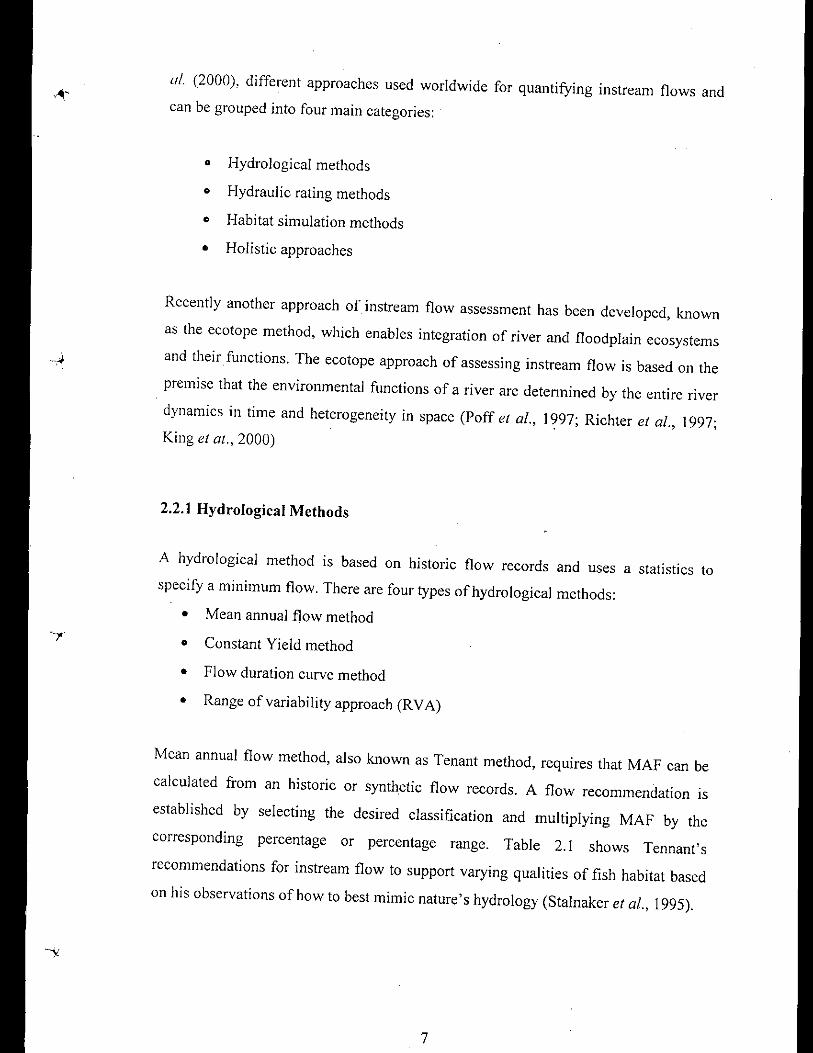
"I. (2000), different approaches used worldwide for quantifying instream flows andcan be grouped into four main categories:
• Hydrological methods
• Hydraulic rating methods
o Habitat simulation methods
o Holistic approaches
Recently another approach of instream flow assessment has been developed, known
as the ecotope method, which enables integration of river and floodplain ecosystems
and their functions. The ecotope approach of assessing instream flow is based on the
premise that the environmental functions of a river are determined by the entire river
dynamics in time and heterogeneity in space (Poff el al., 1997; Richter el al., 1997;King el al., 2000)
2.2.1 Hydrological Methods
A hydrological method is based on historic flow records and uses a statistics to
specify a minimum flow. There are four types of hydrological methods:
• Mean annual flow method
• Constant Yield method
• Flow duration curve method
• Range of variability approach (RVA)
Mean annual flow method, also known as Tenant method, requires that MAF can be
calculated from an historic or synthetic flow records. A flow recommendation is
established by selecting the desired classification and multiplying MAF by the
corresponding percentage or percentage range. Table 2.1 shows Tennant's
recommendations for instream flow to support varying qualities of fish habitat based
on his observations of how to best mimic nature's hydrology (Stalnaker el al., 1995).
7

8
Table 2.1 Percentage of mean annual flow required to achieve different objectivesbased on the Tennant method
The Constant Yield Method (Loar and Sale, 1981) developed in the USA uses a
combination of the median flow and constant yield statistics to represent watershed
hydrology. For unregulated streams with a drainage area greater than 130 km2 and
historic flow records greater than 25 years with a :t 10% accuracy of gauge, the
median monthly flow serves as the datum for evaluating instream flow needs.
Percent of mean annual flowLow flow season
20060-] 004030201010<10
Habitat qualityFlushing or maximumOptimumOutstandingExcellentGoodFairPoorSevere degradation
The Flow Duration Curve (FDC) Method utilizes historical records to construct flow
duration curves for each month to provide cumulative probabilities of exceedance for
various flows. Based on at least 20 years of daily flow records, a flow
recommendation is made for each month. This method includes the provision to
eliminate abnormal events, after which the recommended flow for instream protection
may be set at the 90th percentile (flow equaled or exceeded 90% of the time) for
normal months and the 50th percentile during high flow months. Since the level of
protection is implicit in the magnitude of percentage, different exceedance
probabilities have been used in specifYing flow.
The range of variability approach (RVA), relatively a new methodology (Richter et al.
1996, 1997), is intended for flow target setting on rivers where protection of the
natural ecosystem is the primary objective. It examines the whole river flow regime
rather than pre-derived statistics. A fundamental principle is to maintain integrity,
natural seasonality and variability of flows, including floods and low flows. The
method identifies the important components of a natural flow regime for the river,

indexed by magnitude (of both high and low flows), timing (indexed by monthly
statistics), frequency (number of events) and duration (indexed by moving average
minima and maxima). It uses gauged or modeled discharges, and a set of 32 statistical
parametcrs based upon them (mean annual 7, 30, 60 day minima and maxima, etc.)
may be included. A range of variation of the statistics is then set, based on +/_1
standard deviation from the mean or between the 25'h and 75th percentile. It is
intended to define interim standards, which can then be monitored and revised
(Dunbar et al., 1998; Dayson, et al., 2003).
2.2.2 Hydraulic Rating Methods
Hydraulic rating methods relate various parameters of the hydraulic geometry of the
stream channels to discharge. These are stated to be a little more than basic standard-
setting techniques but not quite incrementa!. One of the most commonly used
hydraulic methods considers the variation in wetted perimeter with discharge. The
wetted perimeter-discharge relationships as shown in Figure 2.1 are constructed from
measuring the length of the wetted perimeter at different'discharges in the river of
interest. The method is based on the assumption that fish rearing is related to food
production, which in turn is related to how much of the river bed is wet. It uses
relationships between wetted perimeter and discharge, depth and velocity to set
minimum discharges for fish food production and rearing (including spawning). The
wetted perimeter technique selects the narrowest wetted bottom of the stream cross-
section that is estimated to protect the minimum habitat needs. The relation of wetted
perimeter to cross-section is shown in Figure 2.1. The analyst selects an area assumed
to be critical for the stream's functioning (typically a riffle). When a riffle is used in
the analysis, the assumption is that minimum flow satisfies the needs for food
production, fish passage and spawning. Once this level of flow is estimated, other
habitat areas, such as pools and runs are also assumed to be satisfactorily protected.
The usual procedure is to choose the break or 'point of diminishing returns' in the
stream's wetted perimeter versus discharge relation as a surrogate for minimally
accepted habitat. This inflection point represents that flow above which the rates of
wetted perimeter gains begin to slow. Because the shape of the channel can influence
9

10
.<
Bank TOll
Ilruk [Hllnu In ~l(lpc
Dischuge
Wetted Perimeter Discharge relationshipTypical river cross-section
Figure 2.1 Relation between wetted perimeter, cross:section and discharge(Source: Bari and Marchand, 2006)
It is relatively a quick and cost-effective method and useful as a planning tool at
catchment scale or greater. Because it is widely used in the United States, there is a
great deal of expertise and experience to draw upon.
2.2.3 Habitat Simulation Method
W.ler level, cllrresp"ndlUJ::10bruk pollll~
the results of the analysis, this technique is usually applied to streams with cross-
sections that are wide, shallow and relatively rectangular.
Habitat simulation methods are the most advanced and an extension of hydraulic
methods. Their great strength is that they quantifY the loss and/or gain of habitat
caused by changes in flow regime, which helps the evaluation of alternative flow
proposals. The aim of habitat based methods is to maintain or even improve the
physical habitat for the biota or to avoid limitations of physical habitat. They require
detailed hydraulic data as well as knowledge of the ecosystem and the physical
requirement of stream biota. Within such methods, changes in physical microhabitat
with discharge are modeled using data on one or more hydraulic variables, most
commonly depth, velocity, substrate, cover and, more recently benthic shear stress
(Tharme, 1996). These data are collected at multiple cross sections within the study
reach. Simulated available habitat conditions are linked with information on suitable
and unsuitable microhabitat conditions for the target species. The final outputs,
usually in the form of habitat- discharge curves for the target biota, are used to predict
optimum discharges as instream flow recommendations.

Tharme (1996) and Dunbar et al (1998) provide an overview of some of the vast
number of habitat rating methods that in the past have been used and in some
instances, still are used to calculate instream flows. Commonly used habitat rating
methods are I) Usable Width method, 2) Weighted Usable Width method and 3)
lnstream Flow Incremental Methodology (IFIM).
Of the available habitat simulation methods, IFIM is considered to be the most
sophisticated and scientifically and legally defensible methodology available for
qualitatively assessing IFRs for rivers (Gore and Nestler, 1998). It is therefore the
most commonly used instream flow methodology worldwide, particularly in the USA
where it was developed (King and Thanne, J 994). The IFIM is an interdisciplinary
framework for the technical side of river flow management. It is termed a
methodology because the framework encompasses more. than one method. It IS
incremental because the procedure is to examine how stream characteristics change
incrementally with flow to determine acceptable levels to compare alternatives. The
evaluation of physical habitat (usually depth, velocity and substrate) is one of the
main components of IFIM, but the process of assessing the impact of varying flow
and determining an appropriate flow regime should be considered whether other
ecologically important characteristics change with flow.
IFIM comprises a set of analytical procedures and computer models, including its
main component, the Physical Habitat Simulation (PHABSIM) model. In its basic
form, PHABSIM comprises two sets of procedures, hydraulic simulation and habitat
simulation. The results of the simulation procedures are linked to produce an output of
Weighted Usable Area (WUA) versus discharge (Figure 2.2), showing losses or gains
in habitat, described by some combination of depth, velocity, substrate and cover, as a
function of discharge for the target species. Breakpoints on the WUA-discharge
curves are used to recommend instream flow.
Recently, several other habitat simulation models similar to and with many of the
same data requirements as the PHABSIM have emerged (Dunbar et aI 1998). The first
of these is the River Hydraulics and Habitat Simulation (RHYHABSIM) program
J I

Weighted Usable Area V5 Discharge
12
500035002000 2500 3000
Discharge (m'/s)
15001000500
Figure 2.2 Weighted Usable Area vs Discharge functions
(Source: Bari and Marchand, 2006)
oo
500000
." 3500000
6'~ 3OOCXXlO
1!'0 2500000E=g 200000o
4500000
developed in New Zealand. It is essentially a simplified version of PHABSIM and
possesses a similar though somewhat reduced scope for application, has similar data
requirement and comprises the same kind of procedure. The Riverine Habitat
Simulation (RHABSIM) is a commercial version of PHABSIM, developed in the
USA by Thomas R. Payne & Associates. It includes the habitat time series program in
addition to other PHABSIM programs. The Computer Aided Simulation Model for
InstreamFlow Requirement (CASIMIR) in regulated streams is a habitat simulation
methodology that has been developed for assessment of instream flows under
condition of hydropower. The River System Simulator (RSS) is a habitat simulation
program system developed in Norway for specific application to rivers regulated by
hydropower schemes. The RSS provides for the integration of several established
hydrological, hydraulic and habitat simulation models, for spatially and temporally
dynamic habitat modeling. The French Evaluation of Habitat Method (EVHA) and
Canadian microhabitat modeling system HABIOSIM are other habitat simulation
methodologies bearing some resemblance ofPHABSIM.
400000o
Habitat simulation methodologies provide a means of assessing instream flows in
situations where competition between instream and offstream uses is likely to be
highly controversial (Estes and Osborn, 1986), or where the river system and some of
its components are of exceptional importance.
As habitat simulation methodologies are able to assess the impact of incremental
changes in flow, and typically have dynamic hydrological and habitat time series
components, they can be used to examine a variety of alternative instream flow
scenarios for several species. Moreover, as they are computer based, they are able to
efficiently process large amount of hydrological, hydraulic and biological data in a
standardized, flexible and interactive manner. In addition, the outputs are produced at
increasingly high degree of resolution, particularly as advances are made in the field
of multidimensional hydraulic modeling. Such modeling more accurately reflects the
hydraulic conditions that are experienced by the biota and by different types of rivers
Stewart (2000) applied two dimensional hydraulic modeling using RMA2 model to
map mesohabitat units, which were then correlated with adult fish abundance
estimated by electro fishing.
Modeling approaches like PHABSIM are sufficiently flexible to enable alternative
hydraulic variables to be incorporated in future, provided that they can be objectively
quantified and that the way their influence changes with increments in discharge can
be accurately modeled. The methodologies are also highly adaptable. For example,
IFIM has been modified for and applied in several new contexts in recent years, such
as instream flows for peaking hydropower and sediment flushing. Advances are being
made in linking the outputs from habitat simulation methodologies with current water
quality and temperature models in more structured and sophisticated ways.
2.2.4 Holistic Approach
Holistic approaches are essentially ways of organizing and using flow-related data
and knowledge. They often incorporate some of the methods described above,
particularly the expert panel methods. They are better described as methodologies,
which implies the linking of several distinct procedures or methods to produce an
13

output that none could have produced alone. The Holistic Method in Australia
(Arthington, 1995, cited in Dunbar el al., 1998) and the Building Block Methodology
(BBM) in South Africa (King el aI., 2000) were developed in collaboration and share
the same basic tenets and assumptions. Both require early identification of the future
desired condition of the river. An instream flow regime is then constructed on a
month by month basis, through separate consideration of different components of the
flow regime to achieve and maintain this condition. Each flow component is intended
to achieve a particular ecological, geomorphologic or water-quality objective.
The family of holistic approach and expert panel based methods has the common
feature that they use a team of experts to make judgments on the flow needs of
different aquatic biota. The composition of the panel will depend on the specific
environmental and social features of the river in question, but typically includes a
hydrologist, geomorphologist, aquatic botanist and fish biologist. In many cases, one
or more community representatives will join the panel. The collective experience of
the panel members is used in the absence of reliable, predictive flow-ecology models.
By putting these experts on a panel, rather than employing them independently, it is
expected that an integrated assessment of flow needs will emerge.
2.2.5 Ecotope Method
To evaluate the impacts of a changed flow regime on the production function an
approach is used in which the concept of the ecotope plays a key role. The concept of
Ecotope originates from landscape ecology and was introduced by Tansley (1939).
Ecotopes are land units that are determined by various aspects and processes
occurring in the landscape. These involve physical aspects such as erosion and
sedimentation, soil development and flooding, as well as vegetation structure and
faunal species including crop growth and fisheries related activities by human.
Applying the ecotope concept thus allows integration of the physical, ecological andlivelihood functions ofrivers.
Such a method seems useful in lowland rivers systems such as in Bangladesh where
the floodplain fonus an intricate part of the riverine ecosystem (Bari and Marchand,
14

15
Remote sensingImages
SRTM LaserAltimetry
ID-2DHydrodynamic
Model
Digital ElevationModel
Remote sensingImages
IRSB&W+IRS Color
Landuse Map
Ecotope Map(future
situation)
Hydrological Data
Fish & Crop yield /Habitat evaluation
Habitat andLandusc
Suitability Rules
Field SurveysVegetation /Crops/ Fish
(ground truthing)
Ecotope modeling framework in setting instream flow requirements
(Source: Bari and Marchand, 2006)
Figure 2.3
2006). They presented the general procedure in thc ecotope approach for assessinginstream flow requirements as shown in Figure 2.3.
2.3 Instream Flow Requirements from Salinity Consideration
Increased salinities and vertical stratification of the water column and penetration of
the salt-wedge farther upstream are attributable to reduced inflows (Peirsoon, et aI,
2002). Salinity not only degrades the water quality to use it as a source of drinking
and irrigation water but also hampers the suitability of the aquatic environment. The
Ecotopc Classificationand Map
(present situation)
Present situation
Future situation
Remote sensingImages
IRS 13&W + RadarFlood

--y
US EPA recognises salinity as a common habitat indicator (abiotic condition
indicator) for use in estuaries. Salinity is well-defined and measurable, and has
ecological significance encompassing a number of estuarine properties and processes(Jassby et aI, 1995).
Corbett (2000) noted the use of an indicator species (Vallisneria americana) to
detcrmine the overall health of the Caloosahatchee River estuary in Florida. The
species was found to be especially sensitive to salinity and its growth steadily declines
with increasing salinity until approximately 8-9 ppt. It will survive in waters with 11-
13 ppt, but its density declines when salinity is over 10ppt. It was determined that
fresh water flows between 400-600 cubic feet per second from upstream keep the
salinity near healthy levels for this species of sea grass at a designated point.
2.4 Related studies in Bangladesh
Research and studies on instream flow is relatively new in Bangladesh and a few
studies have been conducted in recent years. Salinity intrusion is a major problem for
the south west region of the country. Related studies are reviewed in this section.
2.4.1 lnstream flow studies
Assessment of instream flow requirement of the Ganges river based on hydrologic
approach (Rahman, 1998) was the first application of instream flow methods in
Bangladesh. The study shows that the minimum instream flow requirement of the
Ganges is about 1154 mJ Is whereas the observed minimum flow of Ganges ranged
between 221 and 889 mJ/s. The minimum flow during the pre-Farakka was 1190 m3/s
which is found to be very close to the calculated instream flow requirement. Based on
the results obtained, instream flow requirement was indicted to range from 1150 to
2000 mJIs in order to restore and sustain the natural environment of the Ganges.
Zobayer (2004) applied Physical Habitat Simulation (PHABSIM) method to
determine the instream flow requirement of Surma river for three selected fish species
Ghagot, Baghair and Bhaca. The study demonstrates the use of the weighted usable
16

'~.'
area versus discharge function for recommending month wise instream flowrequirements.
Bari and Marchand (2006) applied various methods of instream flow requirements in
Teesta, Surma-Kushiyara and Gorai river in a research undertaken within the
framework of the BUET-Delft University of Technology Linkage Project. They
applied hydrologic, physical habitat simulation and ecotope approach for assessing
instream flow requirements for the selected rivers.
2.4.2 Salinity Related Studies
Environmental degradation in the Sundarban due to deterioration of water eco-
systems was studied under Sundarban Biodiversity Conservation Project (IWM,
2003). The Sundarban Reserve Forest is a complex ecosystem comprising the largest
diversified mangrove forest of the world, located in the southwest region of
Bangladesh. The area in general comprises a coastal flood plain criss-crossed by
numerous rivers, creeks and depressions. The study indicated that the biodiversity has
been affected by the adverse effects of salinity, pollution and siltation in the water and
soil. These adverse situations were said to be due to the insufficient freshwater inflow
to the region, long term effect of global warming and sea level rise. MIKE 11 model
was used for assessing the amount of fresh water inflow required to maintain the
salinity level within tolerable limit in the Sundarban.
Various options for protecting the Ganges Dependant Area from environmental
degradation were studied in the National Water Management Plan (Halcrow and Mott
MacDonald, 2001). The objective of the study was to test the impact of increasing
flow in Gorai, Mathabhanga and other spill channel on the Ganges dependent area
including the Sundarban through implementation of the Ganges Barrage.
In an effort to restore Gorai river by dredging the river mouth to increase inflow from
the Ganges, the Gorai River Restoration Project was taken and pilot scale dredging
was done during 1998-2001 (BWDB, 2000). The overall objective project was to
prevent environmental degradation in the southwest region, specially around Khulna,
17

the coastal belt and in the Sundarban by augmenting Gorai flow and thereby
increasing fresh water flow in the southwest region.
River Research Tnstitute and SWMC (1995) jointly studied to develop the Hydraulic
model for integrated Resource development of the Sundarban reserve Forest. Tn that
study they tried to develop a methodology to provide a qualitative assessment of the
hydraulic parameters like tidal range, ideal circulation and salinity distribution in the
river. The study also tested few options like the impact of Gorai river discharge and
sea level rise inside Sundarban Reserve Forest.
2.5 Choice of Instream Flow Methods
ln choosing an appropriate method for assessing instream flow, understanding of
several factors is required. The purpose of a flow assessment and the intended use of
the results should guide the selection of the assessment method. Project-specific flow
assessments for large or controversial projects, which are likely to call for
considerable negotiation and tradeoffs between environment and development issues,
require a more comprehensive approach than do flow assessments for coarse-scale
planning studies, where a single number might suffice.
Dunbar el al. (1998) observed that given the wide variety of river types and sizes in
existence, it is unlikely that one method could be appropriate in all cases. Since there
is no single all encompassing method, a range of approaches should be appropriate.
They cited Saccardo et al. (1994) who undertook a pilot TFTM/PHABSTMstudy on the
Arzino river and compared with a suite of standard-setting methods, based on daily
and annual mean flows, and flow percentiles.
Since no one method will provide for all needs and required flow assessment should
be reevaluated with changing demands and management strategies, a range of
approaches requiring different levels of expertise and amount of data should beappropriate.
18

~.
2.6 Important Definitions
Definitions of some important terms regarding this study are summarized In thissection.
Instream Flow Requirement (IFR): Instream flow or environmental flow requirements
are defined as those flows that are essential within a stream to maintain its natural
resources and dynamics at desired or specified level.
Salinity intrusion: Salinity intrusion is defined as the introduction, accumulation or
formation of saline water in a water of lesser salinity.
Habitat: A river or a stream which is the living place for many different types of
living organisms is known as habitat.
Weighted Usable Area (WUA): Weighted usable area is expressed as square meter of
habitat area estimated to be available per 1000 linear meter of stream reach at a givenflow.
Substrate preference: Substrate is the bed material of a river or stream. So substrate
preference is the suitability of the bed material for a specific species.
Habitat Suitability Criteria (HSC): The HSC are used to describe the adequacy of
various combinations of depth, velocity and channel index conditions in each habitat
computational cell to produce an estimate of the quantity of habitat in terms of surfacearea.
•
19

Chapter 3
Methodology
3.1 Approach of the Study
Two different Methods were involved in this study to assess the instream flow
requirement of Gorai river. Firstly the one dimensional salinity simulation was
performed considering salinity intrusion for assessing the flow requirement of Gorai
river to keep the salinity within allowable limits for Irigation and household use of
water and to support Sundari tree growth in Sundarban. Secondly the flow
requirement in Gorai river assessed by Bari and Marchand (2006) using PHABSIM
considering two dominant fish habitat, Ayeer and Bacha, was compared with thatassessed from salinity considertations.
The steps of the methodology of this research may be stated as follows:
3.2 Selection of Study Reach
For investigation of salinity intrusion, the entire reach of Gorai river from its
headwaters at the Ganges river upto its downstream limit including the interconnected
river system leading to the Bay of Bengal was considered. For application of
PHABSIM model, about a 26 km reach of Gorai river from just upstream of Gorai
Railway Bridge towards downstream direction was considered (Figure 3. I). Results of
PHABSIM method are available in Bari and Merchand (2006) which was used for
comparison in the present study.

3.3 Data Collection
WJ I~'
Gorai RailwayBridge
21
N
A
Cross-section
''''I'.
"'J'"
2 024,~ .__ .- ----1 kill
Figure 3.1 PHABSIM study reach of Gorai river(Source: Sari and Marchand, 2006)
?:
~.
• For simulation of salinity intrusion, data required include discharge, water
level, cross-sections and salinity concentration at various locations. These data
were collected from BWDB and Institute of Water Modeling as appropriate.
• For PHABSIM modeling discharge, cross-section and depth, velocity and
substrate preference data for dominant fish species are required. These data are
reported in Bari and Marchand (2006).

3.4 Simulation of Salinity Intrusion
Salinity concentration was simulated at various points along the Gorai river from
Bardia to Hiron Point as well as at several locations on Sibsa, Kobadak, Pussur,
Harintana and different interconnected rivers and khals. This was done using the
Salinity module of MIKE II.
Initially a salinity model for Gorai river including the interconnected rivers in the
southwest region was developed by IWM using an MIKE II version 200 I. Later
updated versions of MIKE 11 were available in IWM but they did not recalibrate the
salinity model as there was no specific project for application.
For the purpose of present study this salinity model was recalibrated using MIKE 11
version 2005 and was used for assessment of flow requirement for keeping salinity
concentration within the tolerable limits at different locations for different uses of
water, such as for irrigation, source of drinking water supply, and mangrove forestrequirement.
3.5 Fish Habitat Simulation
Physical Habitat Simulation (PHABSIM) model, first presented by Bovee and
Milhous (1978), discussed by Bovee (1982) and Milhous et al. (1984), is designed to
calculate the amount of habitat available for different life stages of selected fish
species at different flow levels. Habitat is an encompassing ten11 used to describe the
physical surroundings of plants and animals. In the PHABSIM analysis hydraulic
model is used to determine the characteristics of stream in terms of depth and velocity
as a function of discharge for the full range of discharges to be considered. In habitat
modeling process this information is integrated with habitat suitability criteria, i.e.
depth, velocity and substrate preference of selected fish species, to produce a measure
of available physical habitat as function of discharge, known as weighted usable area
versus discharge (WUA-Q) function. This curve is then used to define a flow range or
minimum flow for selected fish species. Bari and Marchand (2006) assessed flow
requirement in Gorai river to support two selected fish species: Ayeer (Aorichthyst ..:"••
22

aor) and Bacha (Eutropiichthys vacha). These results were used for a comparative
analysis of instream flow requirements from alternative functional needs.
3.6 Comparative Analysis of the Instream Flow Requirements Assessed byAlternative Methods
Finally flow requirement of Gorai river assessed from consideration to limit salinity
intrusion and to support selected fish species was compared. Since there is no all
encompassing method that will provide for all needs, it is appropriate to apply
alternative flow assessment methods in order to be able to present alternative flowscenarios to decision makers.
,, .,• •
23

Chapter 4
Instream Flow Requirement Based on SalinityConsideration
4.1 Influence of Salinity intrusion on in-river Functions
Salinity of water restricts its use for irrigation and drinking. Fish habitat availability of
river also changes with salinity according the suitability of specific fish species. Thus
in-river functions not only depend on the quantity of flow but also on salinityconcentration of water.
Salinity is defined as the relative concentration of dissolved salt found in a sample of
water. The salts dissolved in such water, are usually dominated by the carbonates,
chlorides and sulphates of calcium, magnesium and sodium. Seawater has an average
salinity of about 35000 ppm or 35 kg/m3. Salinity is most commonly measured by
salinometer. Generally, the units of salinity are used ~s kglm\ppt), mg/I(ppm),
mmohs/cm, Ilmohs/cm etc., kg/m3 or mg/I indicates the concentration, whereas
mmohs/cm or Ilmohs/cm indicates the electrical conductivity of salinity. The
conductivity of salinity varies with temperature.
4.2 Salinity Intrusion
Salinity intrusion is defined as the introduction, accumulation or formation of saline
water in a water of lesser salinity. Salinity intrusion refers to surface water
contamination while salinity encroachment refers to the contamination of ground
water (Louisiana, 1993).
Mixing of salt and fresh water is directly dependent upon the density difference
between them. At a temperature of 20°C, seawater has a density of about 1025 kg/m3,
whereas freshwater has a density of 1000 kg/m3• Because of its lesser density,
freshwater tends to float on top of the seawater (stratification). Turbulence generated
by the movement of the water over the bed of estuary causes visual mixing, which

tends to breakdown any saline freshwater stratification. The faster the water
movement, the stronger the turbulence and greater the resultant mixing
4.3 Allowable Limits of Salinity
Allowable limit of salinity for growth of Sundari tree in the Sundarban has been stated
as 10-15 ppt (Halcrow-Mott Macdonald, 2001). Water salinity for different uses is
defined by FAa. The allowable limits of salinity as prescribed by FAa are given in
Table 4.1.
-"'\' .Table 4. 1 Classification of saline water..Water class Electrical Salt Type of water
conductivity at concentration
25T(flmohs/cm) (kg/m30r ppt)
Non saline <750 <0.50 Drinking and irrigation
water
Slightly saline 750-3000 0.50-1.50 Irrigation water
Moderately 3000-10000 1.50-7.00 Primary drainage watersaline and ground waterHighly saline 10000-25000 7.00-15.00 Secondary drainage water
~and ground water
Very highly 25000-45000 15.00-35.00 Very saline ground watersaline
Brine >45000 >35.00 Sea water
Source: Soil and Salinity Monitoring Report. 1990-97, SRD1
4.4 Mathematical Simulation of Salinity Concentration
,.,The purpose of this study is to investigate the salinity variation and quantify the
amount of freshwater flow required for keeping the salinity within tolerable range in
the study river system. One-dimensional, unsteady salinity intrusion process in a tidal
estuary is solved using a salt balance equation while the tidal hydrodynamics is solved
25

USIng a system of one dimensional, unsteady flow continuity and momentum
equation. Both tidal hydrodynamic equations and salt balance equations are solved
using implicit schemes of finite difference methods. The tidal hydrodynamics are
calibrated by varying Manning's roughness coefficient and the salt balance equation
is calibrated by varying dispersion coefficient until the model computed values
matches with the measured values of selected variables. Stage-discharge relationships
are used for calibration of hydrodynamic model and salt concentration for salinity
modelling.
For the present study MIKE 11 was used for necessary hydrodynamic and salinity
concentration simulation in Gorai and interconnected rivers in the southwestern
estuary upto Hiron point on Pus sur river.
4.4.1 Basic Modules of MIKE 11
The primary features of the modeling system are its integrated modular struetures and
shared databases for the topographic and time series data. Tne related modules are:
• Rainfall-runoff (NAM)
• Hydrodynamics (HD)
• Advection-dispersion (AD)
Hydrodynamic Module
The hydrodynamic module is the nucleus of the MIKE 11 modelling system and it
forms the basis for most modules, advection-dispersion (AD). MIKE II
hydrodynamic module solves the vertically integrated equations of conservation of
mass and momentum (the Saint-Venant equation).
Data Requirements -- The following data are required for setting up HD module:
• River and channel network
• River cross-sectional data
• Water level and discharge time series for boundaries.
• Time series for lateral inflows.
• Initial conditions (water levels and flows in the entire module area)
26

River network includes the information of
• Shape of the river and channel cross-section
• Length of each river /channel
• Description of the river and channel network, i.e., the location of junctions.
• Catchment areas and drainage.
Advection-Dispersion (AD) module
The module is based on one-dimensional equation of conservation of mass of a
dissolved or suspended material and uses the results of the hydrodynamic module.
MIKE 11 AD module applies two transport mechanisms, advective or convective
transport with the mean volume of flow and dispersive transport for concentration
gradient. The movement of salts in the module depends on flow velocities and the
amount of mixing, which occurs with water of differing salinity.
Data requirements -- The data required for the simulation of AD module are:
• Result file from the hydrodynamic (HD) module, which provides the
discharges and water levels.
• The module boundaries, i.e., water level and discharge boundaries of the
hydrodynamic module must be specified as either open or closed for salinity.
Usually downstream water level boundaries are open connection boundaries
whereas upstream discharge boundaries are closed.
• The initial condition of salinity module, the time series of salinity or
constant salinity concentration needs to be specified in open boundaries,
where salt can either enter or leave the module. In closed boundaries, it is
assumed that no net transport of salt occurs.
Calibration parameters -- In advection-dispersion modeule, the variation of the
concentration of open boundaries depends upon the parameter Km;x, after a change
from outward to inward flow. The physical meaning of the Km;x is that, after the
current reversal, the concentration in the inward flow will be dominated by the
concentrations that occurred in the case of flow removal. Another important
27
-~-
calibration parameter is the dispersion coefficient, D, that is determined by the
function of flow velocity and channel conveyance, which is another turn lead to the
volume of flow passing through the channel section.
4.5 Simulation of Salinity Concentration in Southwest Estuary
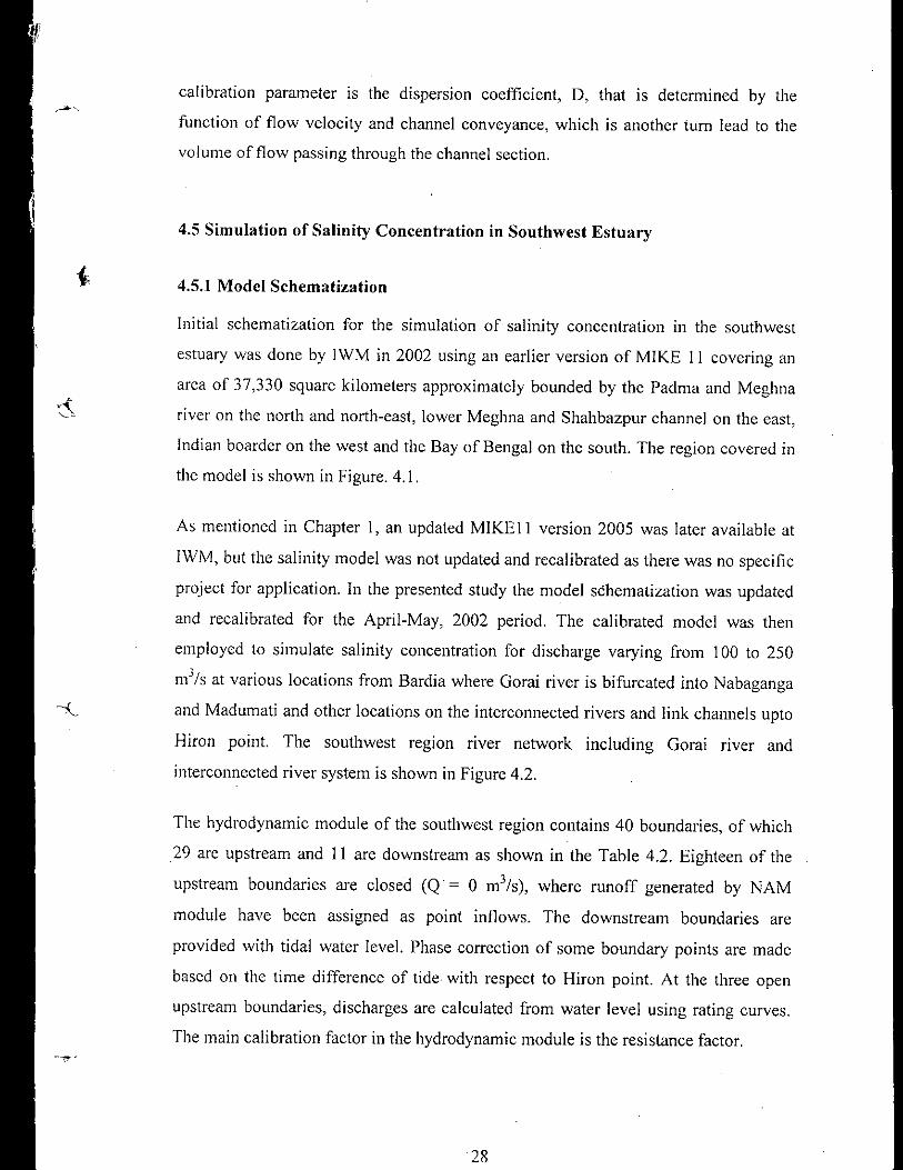
4.5.1 Model Schematization
Initial schematization for the simulation of salinity concentration in the southwest
estuary was done by IWM in 2002 using an earlier version of MIKE II covering an
area of 37,330 square kilometers approximately bounded by the Padma and Meghna
rivel' on the north and north-east, lower Meghna and Shahbazpur channel on the east,
Indian boarder on the west and the Bay of Bengal on the south. The region covered in
the model is shown in Figure. 4.1.
As mentioned in Chapter I, an updated MIKEl I version 2005 was later available at
lWM, but the salinity model was not updated and recalibrated as there was no specific
project for application. In the presented study the model schematization was updated
and recalibrated for the April-May, 2002 period. The calibrated model was then
employed to simulate salinity concentration for discharge varying from 100 to 250
m3/s at various locations from Bardia where Gorai river is bifurcated into Nabaganga
and Madumati and other locations on the interconnected rivers and link channels upto
Hiron point. The southwest region river network including Gorai river and
interconnected river system is shown in Figure 4.2.
The hydrodynamic module of the southwest region contains 40 boundaries, of which
29 are upstream and II are downstream as shown in the Table 4.2. Eighteen of the
upstream boundaries are closed (Q = 0 m3/s), where runoff generated by NAM
module have been assigned as point inflows. The downstream boundaries are
provided with tidal water level. Phase correction of some boundary points are made
based on the time difference of tide with respect to Hiron point. At the three open
upstream boundaries, discharges are calculated from water level using rating curves.
The main calibration factor in the hydrodynamic module is the resistance factor.
28

29
60 Kilometers
I
---J\
LEGEND:
I N-~rirAeo 0i
-••••
.'
N International Boundary
N RiverHyd romaine Stations
• ' Water level
• Water leYeI & Discharge
,------ --------~-------!
-
'.South Wes
Region
o , ,
-~--
1------
I-
I
Figure 4.1 Southwest region location map
(Sollrce: institllte of Water Modelling)
II. /~" , ....•,"! I V1f8 '--'~J I ••~' • , I' \..,)'! "',~, "\~Id,.,'I J ,j', .' :'-,'I.~ iI I! ,r II II iII !I '
:I .,...1,L;_, ---== _=:

Figure 4.2 South west Region showing study river network
(Sollrce: 1nstitllte of Water Modelling)
j_:
!
10 20 )(I i{ij(llndm
Sa.~:
10 0
.......+ + .
e Water Level & Baflrity StatiM!! (IWM)II (8ch8rge. S&d:ment. DO and
Water 0ua6ty Sta1IOM (IVVM)• Wat&r Level Station (Other)II Water level & D1lchmge Station (Other)It> Forestomce
30
LEGEND:
/\/ lntemstional boUnciary/\/ SchemBtized Rtver
m Sundarban Resmv8d Forest
-~-
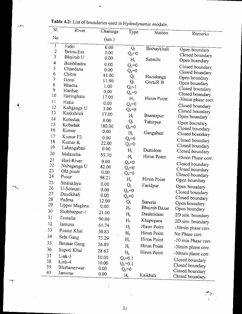
Table 4.2: List of boundaries used in Hydrodynamic module.r~"
SI. River Chainage Type Station RemarksNo (km.)1 Fatki 0.00 Q, Bishaykhali Open boundary2 Betna-Ext 0.00 Qc=O Closed boundary3 Bhairab U 0.00 H, Satmile Open boundary4 Buribhadra 0.00 Qc=O Closed boundary5 Chandana 0.00 Qc=O Closed boundary6 Chitra 41.00 Q, Hazidanga Open boundary7 Gorai II. 90 Q, GoraiRB Open boundary8 Bhadra 1.00 Qc=] Closed boundary9 Harihar 0.00 Qc=O Closed boundary10 Haringhata 17.00 H, Hiron Point -30min phase corr.II Hatia 0.00 Qc=O Closed boundary-{ 12 Kaliganga U 5.00 Qc=O Closed boundary13 Kaskshiali 17.00 H, Bsantapur Open boundary14 Kobadak 0.00 Q, Tahirpur Open boundary15 Kobadak 180.00 Qc=O Closed boundary16 Kumar 0.00 H, Gangabati Closed boundary17 Kumar F2 0.00 Qc=O Closed boundary18 KumarK 22.00 Qc=O Closed boundary19 Labangabati 0.00 H, Oumdom Closed boundary20 Malancha 55.70 H, Hiron Point -45min Phase corr.21 Hari-River 0.00 Qc=O Closed boundary22 Nabaganga U 42.00 Qc=O Closed boundary23 Old pissir 0.00 Qc=O Closed boundary24 Pusur 98.21 H, Hiron Point Open boundary25 Sitalakhya 0.00 Q, Faridpur Open boundary26 U-Solmari 0.00 Qc=O Closed boundary27 Oaudkhali 0.00 Qc=O Closed boundary28 Padma 12.00 Q, Baruria Open boundary29 Upper Meghna 0.00 H, Bhairab Bazar Open boundary30 Shahbazpur-] 21.00 H, Oaulatkhan 20 sim. boundary31 Tentulia 90.00 H, Khepupara 20 sim. boundary32 Jamuna 61.74 H, Hiron Point -30min phase corr." Pussur Khal 30.83 H, Hiron Point No Phase corr.
~~34 Sela Gang 73.29 H, Hiron Point -10 min Phase corr.35 Betmar Gang 36.89 H, Hiron Point -3Omin phase corr.36 Supoti Khal 28.63 H, Hiron Point -30min phase corr.37 Link-3 10.00 Qc=O.1 Closed boundary38 Link-4 10.00 Qc=O.1 Closed boundary39 Bhubaneswar 0.00 Qc=O Closed boundary40 Jamuna 0.00 H, Kaikhali Closed boundaryl'
~iI.
31
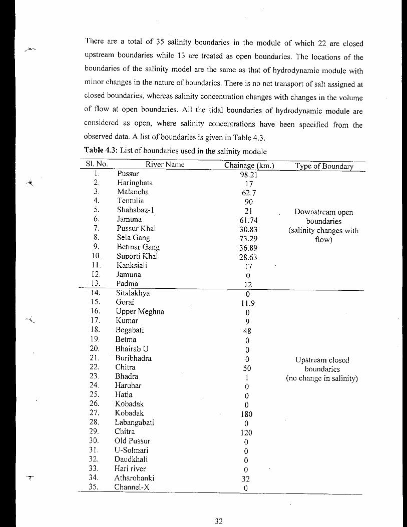
There are a total of 35 salinity boundaries in the module of which 22 are closed-- upstream boundaries while 13 are treated as open boundaries. The locations of the
boundaries of the salinity model are the same as that of hydrodynamic module with
minor changes in the nature of boundaries. There is no net transport of salt assigned at
closed boundaries, whereas salinity concentration changes with changes in the volume
of flow at open boundaries. All the tidal boundaries of hydrodynamic module are
considered as open, where salinity concentrations have been specified from the
observed data. A list of boundaries is given in Table 4.3.
Table 4.3: List of boundaries used in the salinity module
Sl. No. River Name Chainage (km.) Type of BoundaryI. Pus sur 98.21
•••• 2. Haringhata 173. Malancha 62.74. Tentulia 905. Shahabaz-I 21 Downstream open6. Jamuna 61.74 boundaries7. Pussur Khal 30.83 (salinity changes with8. Sela Gang 73.29 flow)9. Betmar Gang 36.8910. Suporti Khal 28.63II. Kanksiali 1712. Jamuna 013. Padma 1214. Sitalakhya 015. Gorai 11.916. Upper Meghna 0
~ 17. Kumar 918. Begabati 4819. Setma 020. Bhairab U 021. Buribhadra 0 Upstream closed22. Chitra 50 boundaries23. Bhadra I (no change in salinity)24. Haruhar 025. Hatia 026. Kobadak 027. Kobadak 18028. Labangabati 029. Chitra 12030. Old Pussur 031. U-Solmari 032. Daudkhali 033. Hari river 0
~'- 34. Atharobanki 3235. Channel-X 0
32

4.5.2 Model Calibration
Calibration of Hydrodynamic Model -- Hydrodynamic module was calibrated for
the period of April-May 2002. Discharge at Gorai Railway Bridge on the Gorai river
and water level at Hironpoint on the Pussur river was taken as upstream and
downstream boundaries respectively. Channel roughness was the controlling
calibration parameter of hydrodynamic module. The M (M=I1n, where n= Manning's
roughness coefficient) values were used as the calibration parameter in the
computation of hydrodynamic module for the river system as shown in the Table 4.4
Table 4.4: Values ofM used in Hydrodynamic module--(.
River Station Distance from Gorai offtake M value
(km) ml/3/sGorai Gorai Railway Bridge 12 30
Nabaganga Bardia 199 35Rupsha Khulna 247 50Pussur Mongla 292 50Pussur Hironpoint 374 60
Calibration of Salinity Model -- In salinity module, the calibration parameters are
Kmixand dispersion coefficient, D. The values of Kmixused for calibration varies from
0.043 to 0.083 and dispersion coefficient, D varies from 10 - 2400 m2/s. The higher
value of dispersion coefficient near the outfall of Pus sur in the Bay of Bengal signifies
that the dispersion process is more significant there than in the upper reaches. The
result from hydrodynamic module was used for the calibration of the salinity module.
The salinity module was calibrated for the period of April-May 2002. Hironpoint on
the Pus sur river was taken as an open boundary with a salinity of 28 ppt and Gorai
railway bridge on Gorai was taken as a closed boundary with zero salinity. The values
of Kmixand dispersion coefficient, D used in calibration is shown in the Table 4.5.
33

Table 4.5: Values of Calibration parameters (Kml>.and D) used in Salinity module.'.l.-- ___
River Station Distance from Gorai Kmix Dmin Dmax
offtake (Km)
Nabaganga Bardia 199 0.083 10 100
Rupsa Khulna 247 10 250
Pussur Mongla 292 200 500
Pussur Hironpoint 374 700 2400
The simulated and observed salinity concentration values in Pussur river at Mongla,
Passakhali and Hironpoint are plotted in Figure 4.3(a), (b) and (c) for May 9-29, 2002,
April 4-24, 2002 and May 4-20, 2002 respectively. In Figure 4.3(a) the observed
salinity values are seen to be slightly higher than the simulated values. In Figure
4.3(b) and (c) observed salinity values are found to fall both below and above the
simulated values. The overall the calibration was reasonably good .
•
34

,~
c-
00:0005-29
00;0004-24
00:0005-20
00;0005-18
.j...
Oh ••.•.•-rdSillIUbr.-d
00:0004-19
00;0005-24
00:0005-16
_.~,..
............. Om,c •••.t'dSb.ulahod
00:0005-14
....J
00:0004.14
,.......--'T'"
Time
00:0005-12
00;0005-19
Tim,
.; - .__ !.
00:0005-10
00:00Q4.<)9
(a) Pu:\s:urRiver at Mongla (Ma~' 9-29. 20(2)
(b) PlIS')Uf Rivet al Pas~lkh•.l[i(ApriI4-24. 20(2)
Time
(c) PUSSUf River III Hiron P<linl(M,y 4-20.20(2)
00;0005-14
00:00054)8
""--.j ..•..
00:0005-06
00:002002-<>4-04
....... - .. f ....
: ! ! c! "
I' ~l:R r 1\ 11\ i' rJ" "/vv\jVlJ''r,!\/Vv.VVV''rjJ,,J\/\/V\P,fvVVV'\/V\!\JyJ\/V \/~\iV\/IJV'J'v v VL'U ! [J ! ! .._- ..!._... - - - ..- --, - _- . -'.' - _, ..
30r----;----~---~---~-----C----,--- -,
20
18
16
= 14nEo
~ 12
!l 10
8
6
4
2
00;002002-05-09
10
00:002002..()5..()4
35
5
20
25
15
!"~ 10
I.~' 1S _ i
"~
Fig 4.3 Comparison of Simulated and Observed Salinity of Pussur river at Mongla,
Passakhali, and Hiron point on indicated date and time

4.6 Effect of Incremental Changes of Flow on Salinity Intrusion
The options for this simulation scheme is given below in Table 4.6. The first two
options were selected to quantify the minimum amount of flow required through the
Gorai river for keeping the salinity level upto Khulna station within tolerable range
for irrigation and drinking water uses. The third and fourth options were selected to
quantify the minimum amount of Gorai river flow required to keep to salinity in the
allowable range for Sundari tree growth in the Sundarbans.
The discharge of Gorai river has a considerable impact on the salinity intrusion
process in southwest estuary. Reduced freshwater flow through Gorai has led to
significant changes in the salinity regime. For investigation the effect of changing
flow regime on salinity concentration, the dry season of 2001-02 was considered as
base condition. During this period the salinity concentration at Khulna was observed
to be 5.924 ppt corresponding discharge of 6.7 m3/s in Gorai at Gorai railway bridge.
The salinity concentration at different locations were simulated for discharge values
of 100, 160, 200 and 250 m3Is at Gorai railway bridge
Purpose
Safeguard irrigation
and household use
Safeguard Sundari tree
Description
Minimum observed discharge 6.7 m3 Is inGorai river at Gorai Railway Bridgedruring April-May 2002
36
Minimum discharge of200 m3/s at GoraiRailway Bridge
Minimum discharge of 160 m3/s at GoraiRailway Bridge
'Minimum discharge of 100 m3 Is at GoraiRailway Bridge
2
3
4 Minimum discharge of250 m3/s at GoraiRailway Bridge
Option
No.
Basecondition
Table 4.6 Options selected for simulation of salinity concentration
-l(,

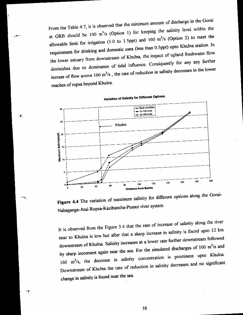
4.7 Results of Salinity Simulation
For four chosen options of upland freshwater flow (100 mJ/s, 160 mJ/s, 200 mJ/s and
250 mJ/s), salinity simulation for southwest region was conducted to assess the
minimum amount of Gorai flow required for two different purposes:
• To keep the salinity level upto Khulna station within allowable limits for
irrigation (1.0 to 1.5 ppt) and as a source of drinking water (less than 0.50
ppt).• To keep the salinity within the allowable range (10.0 to 15.0 ppt) for Sundari
tree growth in Sundarban.
The simulated salinity concentration values at different locations including
Nabaganga at Bardia, Rupsa at Khulna, pussur at Mongla and Hiron point for Option
1 and 2 together with the base condition are presented in rable 4.7. these simulated
values of salinity concentration from Bardia to Hiron point are plotted in Figure 4.4.
37
38
20016016014080 100 120
Distance from Bardla60402Q
oo
5
Variation of Salinity for Different Options
It is observed from the Figure 3.4 that the rate of increase of salinity along the river
near to Khulna is low but after that a sharp increase in salinity is found upto 12 km
downstream ofKhulna. Salinity increases at a lower rate further downstream followed
by sharp increment again near the sea. For the simulated discharges of 100 m3
/s and160 m3Is, the decrease in salinity concentration is prominent upto Khulna.
Downstream of Khulna the rate of reduction in salinity decreases and no significant
change in salinity is found near the sea.
Figure 4.4 The variation of maximum salinity for different options along the Gorai-
Nabaganga_Atai-Rupsa-Kazibancha-Pussur river system
25
1i:2Qic
m 15E,E"~10
From the Table 4.7, it is observed that the minimum amount of discharge in the Gorai
at GRB should be 100 m3/s (Option 1) for keeping the salinity level within the
allowable limit for irrigation (1.0 to 1.Sppt) and 160 m3/s (Option 2) to meet the
requirement for drinking and domestic uses (less than O.sppt) upto Khulna station. In
the lower estuary from downstream of Khulna, the impact of upland freshwater flow
diminishes due to dominance of tidal influence. Consiquently for any any further
incrase of flow avove 160 m3Is , the rate of reduction in salinity decresses in the lower
reaches of rupsa beyond Khulna.

Next, simulation results for keeping the salinity concentrations within the allowable
range (10.0 to 15.0 ppt) to support Sundari tree growth in Sundarban is presented in
Table 4.8 along with the base condition.
Table 4.8: Simulated salinity concentrations for Option 3 and 4
Simulated maximum salinityRiver (ppt) during April-May for
Place (Chainage) Reach Location indicated flowBase Option-3 Option-4
Condition Q=200 Q=250
Q=6.7rnJ/s rn3/s rn'/s
Ji', Nalianala Sibsa Northwest 18.020 17.024 16.708(21915.00)
Mongla Pussur Upper North 14.326 12.055 11.416(16835.00) Sundarban
Mrigamari Mrigamari Northeast 15.547 13.797 13.29(8300.00)
Kaikhali Jamuna Northwest 24.700 24.697 24.695(0.00)
Kobadak Kobadak Northwest 24.191 24.124 24.102(244000.0) Middle
Nandbala Pussur Sundarban Center 15.598 13.871 13.37(31000.00)
Harintana Harintana K East 15.436 15.115 15.000(3600.0)
Hiron piont Pussur South 26.323 25.885 25.818~ (98210.00)
Katka Betmargang3 Lower Southeast 19.547 19.542 J 9.540(6890.0) Sundarban
Supoti Supoti East 12.572 12.567 12.564(0.00)
In Table 4.8 maximum salinity at different locations of Sundarban are presented from
simulation result for two different discharges: 200 m3/s (Option 3) and 250 m3/s
(Option 4) at Gorai Railway Bridge. It is observed that the discharge of Gorai does
not have any major effect in the salinity of the east and west part of the Sundarban but
it has a significant impact on the salinity of the central part of the Saundarban. Due to
the presence of Bay of Bengal and impact of tide, the salinity at the lower boundary of
the Sundarban does not vary too much with the fresh water flow from upstream. As--"(.
there is no major source of freshwater at the western part of Sundarban the salinity of
that zone remains almost unchanged and the value is much higher than the critical
39

J.
j
range for sundari growth (10.0 to 15.0 ppt). Although the Gorai flow don't have any
significant impact on the salinity in the east part of Sundarban but the discharge of
Baleswar keeps the salinity of that zone within the acceptable limit for sundari
growth.
40

Chapter 5
Comparison of Flow Requirements Based on Salinity andFish Habitat
5.1 Introduction
In Chapter 3 flow requirements in Gorai River was assessed to maintain salinity
concentrations within specified limits to safeguard irrigation and domestic uses upto
Khulna and to support growth of Sundari tree in the Sundarban. In a recent study Bari
and Marchand (2006) investigated flow requirements to support selected fish species
considering a 26 km reach of Gorai river starting from just upstream of Gorai Railway
Bridge towards downstream direction. In this chapter efforts are made to make a
comparison of flow requirements obtained from these alternative considerations.
Firstly physical habitat simulation procedure for selected fish specIes usmg
PHABSIM model is briefly presented. Then the results obtained by Bari and
Marchand (2006) for Gorai river considering two species Ayeer (Aarichthys aar) and
Bacha (Eutrapiichthys vacha) are discussed. Finally flow requirement for alternative
functions, such as salinity control and support fish habitats are compared.
5.2 Insteam Flow Assessment using PHABSIM Method
Habitat simulation using PHABSIM compnses two sets of procedures: hydraulic
simulation and habitat simulation. PHABSIM is a specific model designed to
calculate an index to the amount of microhabitat available for different life stages at
different flow levels. The results of the simulation procedures are linked to produce an
output of Weighted Usable Area (WUA) versus discharge. Application of PHABSIM
involves four basic steps: (I) Study site selection and representation, (2) Development
of habitat suitability criteria, (3) Hydraulic simulation and (4) Habitat simulation.

Study Site Selection and Representation
The criteria that have to be taken into account in selecting the study sites include: (i)
availability of a discharge measuring station, cross-section and other hydraulic data,
and (ii) a stream segment having fish potential. Two approaches are available to select
a study reach for PHABSIM. One is representative reach approach in which a reach of
is selected approximately 10-IS channel widths in length and is assumed to contain all
of the mesohabitat types of the river segment (Bovee, 1982). Another is mesohabitat
type approach for irregular distribution of meso habitat throughout the reach Morhardt
el at. (1983). The stream segment is represented by a synthetic reach developed using
the data collected on each mesohabitat type, weighted by the proportion of the
mesohabitat type in the stream segment (Zobeyer, 2004).
Development of Habitat Suitability Criteria
Successful implementation of PHABSIM requires the acquisition and realistic habitat
suitability criteria for the selected species. The basic form for the expression of
suitability is a habitat suitability curve, or other categories of curve called utilization
curves or preference curves. The habitat criteria are derived from life history studies
in the literature, based on frequency analysis of microhabitat conditions utilized by
different life stages and species or from professional experience and judgment.
Suitabilty curves developed for Ayeer and Bacha for Gorai river are given inappendix A.
Hydraulic Simulation
PI-IABSIM has two major analytical components: stream hydraulics and life stage-
specific habitat requirements as shown in Figure 5.1. The stream hydraulics
component predicts depths and water velocities at specific locations on a cross-section
of stream. Field measurements of depth, velocity, substrate material and cover at
specific sampling points on a cross-section are taken at different flows. Hydraulic
measurements, such as water surface elevations, are also collected during the field
inventory. These data are used to calibrate the hydraulic models. The models are then
used to predict depths and velocities at flows different from those measured. The
42

DepHI (ft)
l1Jo I ! J .l
B: "Hahilul Suil:Jhilil.\' criteria
Ion
L'[TIo,~ _ll,~
lo..!
V', 11.2"
0,0Q I 1 .\ ~
Velociry (rtlscc)
II
~t~[Ill,n.:
" ,0 1 .1 ~ X lij
'-- (_;'_",.cr_'_"_"_li,O_"_, J}~------
C; Sellson:!1 relation Ill'tween disl'll:lr~('H1H.OUUanti mi{:mhnhit:lt rur cal'll life st.age
I'HABSJi\1
Crllss se(:lion n
~,III ,m"~II, : . , I ,
)) IIIIIIII! IIV'I vi \'} _~__. V('I,,<I,)"
I)] n~II,' 1l0l'lh
Cl .:: '-'.1 COl",-r.'1 "1.\.' ~ .._ 1\'00
IL , _---------
hydraulic models have two major steps. The first is to calculate the water surface
elevation for a specific flow, thus predicting the depth. The second is to simulate thevelocities across the cross-section
Figure 5.1 Conceptualization of PHABSIM procedure of developing discharge
versus habitat value curve (Source: Stalnaker et al. 1995)
43
Habitat Simulation
In the habitat modelling process the relation of depth and velocity with discharge
determined by hydraulic modelling is integrated with habitat suitability criteria to
produce a measure of available physical habitat as a function of discharge.
Habitat Model Computational Cells --Figure 5.2 shows a generalized representation
of a river segment for a transect that define a matrix of habitat cells with their
associated attributes of depth, velocity and substrate. The hydraulic models simulate
depths and velocities, dl, d2, VI and V2 as shown in Figure 5.2 at the verticals used inthe habitat models.

44
V2
Idi =(d] + d2)!2
Vi =(V] + V2)/2
WUA = I.A,*C;:1
The combined suitability of the cell is derived from the component attribute of each
cell which is evaluated against the species and life stage' habitat suitability curve
coordinates for each attribute to derive the component suitabilities as illustrated in
Figure 4.3, Once the individual component suitabilities have been determined, these
are then aggregated into single composite cell suitability,
Figure 5.2 Matrix of habitat cell attributes in a PHABSIM study
(Source: Zobeyer, 2004)
The 1110stcommon method is to use multiplicative composite index given by:Ci = Vi*Di*Si
where, Ci = composite suitability of cell i
Vi = suitability associated with velocity in cell i
Di = suitability associated with depth in cell i
Si = suitability associated with substrate in cell i
Once the composite suitability index Ci has been determined, then the amount of
WUA using all cells at this specific discharge is computed according to the followingequation:
where, WUA = total weighted usable area in stream at specified discharge
Ai = surface area of cell i
Ci = combined suitability index of cell i (composite of depth, velocity and
channel index individual suitabilities)

Depth
Velocity
Channel index
//
/I
,/
//
,/
o
Di
o
o
Vi
SiChannel index i
Figure 5.3 Habitat suitability criteria attributes for a habitat cell, showingmultiplicative aggregation option (Source: Zobeyer, 2004)
45
This procedure is repeated for a range of discharges to obtain a WUA versus
discharge function. WUA is expressed as square meter of habitat area estimated to be
availableper 1000 linear meter of stream reach at a given flow. Figure 5.1 (c) is an
example of a typical habitat versus flow function showing how incremental changes
in flow result in quantifiable changes in habitat values.
Habitat Time Series Analysis --The major premise of habitat time senes is that
habitat is a function of stream flow and that stream flow varies over time. The basic
steps to calculate habitat time series are illustrated in Figure 5.4 where the habitat
versus flow function (WUA vs. discharge) is integrated with the flow at each time
step to derive habitat availability at each time step. The habitat time series can be
analyzed to derive a habitat duration curve. 0...•-

46
(B)
DischargeQ1
Time
Time
"
"
A1
Figure 5.4 Ingredients for constructing habitat time series: (A) the dischargeassociated with a time step is read from the hydrologic time series, (B) the WUA forthe selected discharge is obtained from the habitat-discharge relationship and (C) theWUA for the time step is entered into the habitat time series.
(Source: Bari and Marchand. 2006)
Habitat Duration Analysis -- A duration curve, whether for flow, habitat or another
instream variable, displays the relationship between the variable and the percentage of
time it is exceeded. Duration curves are constructed by sorting the data (time series or
habitat values) from highest to lowest and expressing each data point as a percentage
of total number of values. These methods are of particular use in the analysis of how
varying and alternative flow regimes affect habitat available to individual life stage of
a species. Figure 5.5 illustrates the concept of habitat duration analysis which
summarizes the availability of habitat values across time under baseline condition,
with projects and after mitigation of project impacts. This information makes it
possible to analyze the effects of changes in flow on each life stage of every species
for which habitat suitability data is available.

Units of availlable hahilat
47
5.3 Results of PHABSIM Simulations
1'"I ..... Bast~linc
: - -----}Ji,.o'1 leel "-;11
! """',. "0" ~
1\L--- !~)l."~___ •L
---h1
0;03.006.2 9.3 12.4 15.518.6 21.724.S27.93 .0
Figure 5.5 Duration analysis of habitat available under baseline conditions, with-project and after mitigation of project (Source: Bari and Marchand, 2006)
The PHABSIM Simulation results of two selected fish species, Ayeer and Bacha is
presented in the form of WUA vs. discharge graph in Fig. 5.6 for the discharge values
from 20 m3/s to 3500 m3/s. The optimum WUA being observed corresponding to 400 .
m3/s and 1000 m3/s of flow for Ayeer (Aorichlhys aor) and Bacha (Eulropiichthys
vacha) respectively. Also habitat time series for each of 12 months for the selected
species are presented in Figure 5.7. From this figure it is seen that the maximum and
minimum mean habitat values for Ayeer occur in August and October and for Bacha
in August and March, respectively.
100...••..-- 90 -
SO -
70 --."~'tl 60 -
'"-" 50'"""'"" 40 -:;
30 ----'" 20 -::':< 10 -
0

4000350030001500 2000 2500Discharge (m'/s)
1- Ayeer - Bacha I
Weighted Usable Area vs Discharge
I
r, ;
; l;L I , I
Jul Aug Sep Oct Nov Dec Jan Feb Mar
ISAyeer IDBacha I
1000500
~ 300000jj 250000S8 200000S8. 150000
NS 100000~~ 50000
oo
500000
450000
50000
oApr May Jun
48
IVJl;;lUIIV1UllUUY ruwmnlOf t'l.yl;;tll
~400000i~350000~•= 300000~!250000~~ 200000;C•; 150000
i100000••
Figure 5.6 Weighted Usable Area vs Discharge functions for Ayeer and Bacha fish
(Source: Bari and Marchand, 2006)
Figure 5.7 Mean monthly habitat for Ayeer and Bacha fish
(Source: Bari andMarchand, 2006)

The ranges of the computed flows for 50"' and 75th percentile values of WUA are
summarized in Table 5.1 for high flow, intermediate flow and low flow months. The
bottom row of Table 5.1 shows that the maximum amount WUAs are obtained at
discharge values of 400 m3/s and,! 000 m3/s, respectively for Ayeer and Bacha fish.
Table 5.1 Flow (m3/s) for indicated species for various exceedence probabilities ofWUA in different seasons of the year at Gorai river
WUA (m'/ 1000 m Flow (m'/s) for indicated fish speciesSeason reach length) Ayeer Bacha
High flow (Jun, Jul, 50'" percentile 660 - 1900 1310-1920Aug, Sep) 75'10 '1 891-2500 1402-2530percentt e
Intermediate flow 50thpercentile 194-1610 194-1630(May, Oct) 75'10percentile 107-2280 106-2310
Low flow (Apr, Nov, 50'" percentile 120 -300 117 -750Dec, Jan, Feb, Mar) 75'10percentile 46-256 46-597
Optimum 400 1000
5.4 Comparative Analysis
An instream requirement depends on different in-river functions: Different approach
emphasizes on different functions. To include more river function in consideration it
is better \0 use alternative methodologies for the assessment of flow requirements.
Instream flow assessment based on alternative approaches, to limit salinity intrusion
and to support selected fish species, are compared.
Considering salinity, the freshwater flow requirement in Gorai for specified uses are
presented in Table 4.7 and Table 4.8. From fish habitat considerations, flow
requirement corresponding to indicated exceedence probalities of WUA are presented
in Table 5.1.
Salinity simulation result shows that minimum discharges of 100 m]/s and 160 m]/s of
Gorai is required respectively to keep the salinity within allowable limits for
irrigation, drinking and domestic uses of river water at Khulna station, whereas a
discharge of about 250 m3/s is needed to maintain salinity level within tolerable limits
49

to support Sundari tree growth for the part of Sundarban forest influenced by Gorai
river flow.
On the other hand physical habitat simulation for two selected fish species, Ayeer
(Aorichthyaor) and Bacha (Eutropiichthes vacha), yielded 400 m3/s and 1000 m3/s
of Gorai flow respectively for optimum habitat condition. During low flow months
when the salinity value remain maximum and considering 75th percentile vale of
WUA, the flow requirement for Ayeer is 256 m3/s and for Bacha is 597 m3/s.
Thus flow requirement of Gorai river considering salinity intrusion falls within that
obtained by habitat requirements for selected fish species, Ayeer and Bacha. The
minimum flow requirement to sustain Sundari tree growth in Sundarban is 250 m3/s
which approaches to the upper value of flow requirement for Ayeer fish. The flow
required for Bacha yielded 597 m3/s which suffices both habitat and salinity
requirements.
Since there is no all encompassmg method that will provide for all needs, it is
appropriate to apply alternative flow assessment methods considering prevailing
problems and functions of a river in order to be able to present results and alternative
scenarios to the decision makers.
5.5 Limitations of the Study
The limitations of the study are as follows:
• In the salinity model it is assumed that substance (salt) is completely mixed
over the cross-section, implying that a source/sink term is considered to mix
instantaneously over the cross-section.
• Only two values of salinity concentrations over a day were available for input
at boundary points. More observations during a day would improve the
salinity simulation results in tidal rivers.
50

• In the hydrodynamic model vertical acceleration is neglected and a static
pressure variation along the vertical is assumed. The computation of salinity
model is sensitive to the computation of discharge in the hydrodynamic model.
As hydrodynamic model is not accurate to mimic the actual situations, the
salinity model has got some obvious limitations to reproduce the salinity
concentrations as observed at different locations.
• Cross-sections of some rivers were not concurrent for the period of discharge
and in some rivers only a few cross-sections were available to represent the
river reach. Discharge and cross-sections for concurrent periods and of recent
years and closer intervals would improve simulation results.
51

•...;-~,~~~~ .<
~",. .I.J"
Chapter 6
Conclusions and Recommendations
6.1 Conclusions
In this study an attempt was made to assess the flow requirement in Gorai river, the
main source of fresh water in the southwest region of Bangladesh, to limit the salinity
within allowable limits for irrigation and domestic uses and to support Sundari tree
growth in Sundarban area. The results are compared with the flow requirements
obtained considering dominant fish species.
From the study, the following conclusions can be drawn:
• Usually the maximum salinity occurs in April and early May, at the end of dry
season. During this time the water is neither usable as a source of drinking
water nor for irrigation even at Khulna which is 127 km upstream from the
coast. The discharges required at Gorai railway bridge to keep the salinity
within the acceptable limits for above uses were found 160 mJ Is and 100 mJ Isrespectively.
• The Gorai flow is not the only influencing factor to control the salinity of
SUndarban for the sustainability of Mangrove forest, the other factors of
influence being tidal phenomenon in the lower estuary and discharges from
other upland freshwater sources. A flow of250 mJ/s of Gorai at Gorai railway
bridge reduces the salinity only of the central part of Sundarban to acceptable
limits of Sundari tree growth.
• The PHABSIM simulation shows a range of discharges for two dominant fish
species-Ayeer and Bacha. For 751h percentile value of WUA the required
discharge are 256 ml/s and 597 ml/s respectively .

~.--
• Alternative methods give a range of flow requirement values for selected
purposes. Considering salinity intrusion and fish habitat a range of instream
flow requirement values can be obtained. It shows that the habitat requirement
for the selected species Bacha (597 ml/s) suffices both requirements as a
source of irrigation, domestic uses and to support Sundari tree growth. Such an
approach of instream flow requirement enables analyst to present a range of
alternatives for the decision makers to choose.
6.2 Recommendations
On the basis of this study, the following recommendations can be made for further
studies:• This study was limited to the impact of Gorai riv,er discharge only. As the
South west region of Bangladesh is very complicated with intricate
interconnected river system comprising tidal channels, further studies would
provide better insight considering the impact of discharges from other sources
offreshwater, specially for the western part of the region
• In this study the MIKE 11 salinity model was calibrated for two months April
and May only considering the extreme buildup of salinity during this time. A
model considering more months would enable to characterize the variation of
salinity concentration with the seasonal changes of freshwater flow
• For PHABSIM, 26 km upstream reach of Gorai was considered in this study.
Efforts may be made to extend physical habitat modelling to assess instreaml
environmental flow requirement in estuaries.
53

References
Arthington, A.H., Pusey, D.R., Bluhdorn, S.E., Bunn, S.E, and King, J.M., 1995. AnHolistic Approach for assessing the environmental flow requirements of riverineecosystems: origins, theory, applications and new developments. LWRRDC andMDBC Workshop on Instream Flow Methodologies, Coomah, ACT, Jun
Bari, M. F. and Marchand, M., 2002, Baseline report, Management of rivers forinstream requirement and ecological protection, BUET, TUDelft, Delft hydraulics.
Bari, M. F. and Marchand, M,. 2006, Management of rivers for instream requirementand ecological protection, Final Technical report, BUET-DUT Linkage Project,Research project-2, BUET, TUDelft.
Bovee, K.D.,1982, A guide to stream habitat analysis using the instream flowincremental methodology. Instream Flow Information Paper 12. U.S Fish andWildlife Service FWS/OBS-82126.
Bovee, K.D., and Milhous., R. T., 1978. Hydraulic simulation in instreamflowstudies: Theory and Techniques. Instrcam Flow Information Paper 5. U.S Fish andWildlife Service FWS/OBS-78133.
BWDB, 2000. Environmental baseline of Gorairiver restoration project, Environment& GIS Support Project for Water Sector Planning (EGIS). .
Dayson, M., Bergkamp, G., and Scanlon, J. (eds)., 2003. Flow-The Essentials ofEnvironmental Flows. IUCN, Gland, Switzerland and Cambridge, UK.
Dunbar, MJ., Gustard, A., Acreman, M.C., and Elliot, C.R., 1998. OverseasApproaches to Setting River Flow Objectives, R&D Tech Report W6-161, Institute ofHydrology, Wallingford, UK, Dunbar, MJ., Gustard, A., Acreman, M.C., and Elliot,C.R., 1998. Overseas Approaches to Setting River Flow Objectives, R&D TechReport W6-161, Institute of Hydrology, Wallingford, UK.
Estes, C.C. and Orsborn, J. F., 1986, Review and analysis of methods for quantifyinginstream flow requirements. Water Resources Bulletin 22(30:389-398), AmericanWater Resources Association.FPCO, 1994, Fishpass pilot project implementation plan, Northeast regional WaterManagement Project (FAP 6).
Gordon, N.D., McMahon, T.A., and Finlayson, B.L., 1992. Stream Hydrology. AnIntroductionjiJr Ecologists, John Wiley & Sons, Ltd., Chichester.
Gore, J. A., and Nestler., J. M., 1988. Instrcam flow studies in perspective. RegulatedRivers: Research and Management.

Halcrow and Mott MacDonald, 2001. Option for the Ganges Dependent Area, DraliFinal Report, Volume 5, Water Resources Planning Organization, Ministry of WaterResources, Government of People's Republic of Bangladesh.
IWM, 2003, Surface Water Modelling of Sundarban Biodiversity ConservationProject, Final Report, Volume-I, Department of Forest, Government of People'sRepublic of Bangladesh.
Jowett, I.G., 1997. In-stream Flow Methods: A Comparison of Approaches RegulatedRivers: Research and Management.
King, J M., Tharme, R.E., 1994, Asessment of Instream flow IncrementalMethodology and initial development of alternative instream flow methodologies forSouth Africa. Water Resource Commission Report no. 295/1/94. Water ResourceCommission, Pritoria.
King, J M., Tharme, R.E., and de Villiers, D.E., 2000. Environmental FlowAssessments for Rivers: Manual for the Building Block Methodology, FreshwaterResearch Univ, University of Cape Town, WRE Report No. TT 131/00.
Loar, J.M., and Sale, MJ., 1981. Analysis of Envirorunental Issues Related to Small-Scale Hydroelectric Development, Instream Flow Needs for Fishery Resources,Puhlication No. J829, Oak Ridge National Laboratory, Oak Ridge, Tennessee.
Lousiana, USA, 1993, Non Point Source Pollution Assessment Report, Water QualityAssessment Plan.
Milhous, R.T., Wagner, D.L., and Waddle., T., 1984. User's guide to physical habitatsimulation system, US Fish and Wildlife Service Biological Services Program,FWS/OBS-81/43.
Ministry of Water Resources, 1999, National Water Policy, Bangladesh
Peirson, W L, Bishop, K, Van Senden, D, Horton, P Rand Adamantidis, C A., 2002,Technical Report Number 3, Environment Australia.
Poff, N.L., Allan, J.D., Bain, M.B., Karr, J.R., Prestegaard, K.L., Richter, B.D.,Sparks, R.E., and Stromberg, J.C., 1997. The natural flow regime in Bioscience 47.
Rahman, M., 1998, A hydrologic determination of instream flow requirement of theGanges River, M. Engg. Thesis, Department of Water Resources Engineering,Bangladesh University of Engineering and Tech.
Richter, B.D., Baumgartner, lV., Powell, J., and Braun, D.P., 1996. A method forassessing hydrological alteration within ecosystems, Conservation Biology.
Richter, B.D., Baumgartner, lV., Wigington, R., and Braun, D.P., 1997. How muchwater docs a river need? Freshwater Biology.
55

RRI & SWMC, 1995, Intrigated Resourse Development of the Sundarban ReserveForest, Hydraulic Modelling Stydy, Ministry of Water Rcsourecs, Govcrnmcnt ofBangladcsh.
Stcwart, G.B., 2000, Two dimcnsional hydraulic modclling for making instrcam flowrecommendations. M.Se Thesis, Dcpartment of Earth Resources, Colorado StatcUniversity, Fort Collins, Colorado.
SWMC. 2000, Surveys and Mathcmatical Modelling to Support the Design Work ofGorai Rivcr Restoration Project, Draft Final Report, Volumc III, Bangladesh WaterDevelopment Board, Ministry of Water Resources, Government of Bangladesh.
SWMC, 200 I, Environmental and Social Impact Assessmcnt of Gorai RiverRcstoration Project, Salinity Model Rcport, GRRP, Bangladesh Water DevelopmentBoard, Ministry of Water Resources, Government of Bangladesh.
Stalnaker, c., Lamb, B.L., Henriksen, J., Bovee, K., and Bartholow, J., 1995. TheInstrcam Flow Incremental methodology, A Primer for IFIM, Biological Rcport 29,National Biological Service, U.S. Department ofInterior, Washington, D.C. March.
Tenslcy, 1939, The British islcs and thcir vcgetation. Cambridgc University Press.
Thame, R.E., 1996, Review of international methodologies for the quantification ofthe instream flow rcquirements of he river, Water Law Review Report, for PolicyDevelopment, Freshwater rcsearch unit, Zoology Department, University ofCapetown, South Africa.
WARPO, 200 I, National Water Management Plan, Ministry of Watcr Resources,Bangladesh.
Zappia, H. and Haycs, D.C., 1998, A Demonstration of Instream Flow IncrementalMethodology, Shenandoah River, Water-Resources Investigation Report.
Zobcyer, A.T.M.H., 2004, Application of physical habitat simulation approach forinstream flow rcquiremcnt in the Surma rivcr, MSc. Engineering thesis, Dept ofWater Resources Engineering, Bangladesh University of Engineering & Technology.
56

200
200
1eo
180
100
180
Hiron point
140
Hiron point
140
.....-Mongla
80 100 120
D1atance fJ"Om Bardla(km)
80 100 120Distance from Banlia(km)
....--Mongla
60
80
+-- Khulna
....-- Khulna
40
4020oo
5
5
oo
25
10
30
Comparison of MIKE11 Version 2001 and 2005 Results
35
Comparison of MIKE11 Version 2001 and 2006 results
.....- MIKE11(2005)-MIKE11(2001)
_ MlKE11 (2CXJ5)_MIKE11(2001)
Appendix A
30
~ .--Bardia"20
i~B 15
i
25
!20 .....-Bardia
~c
i 15E~J
10
Figure A.1(b) Comparison of MIKE 11 version 2001 and2005 results for Q=lOO m3/s.
Figure A. 1(a) Comparison of MIKE 11 version 2001 and 2005 results for base condition

12
---- -- ----- --II
Ii
10
---- ---- .... --- ... -.,'. I
0_8
8
0_6
6
Depth (m)
--._....._-_.__ .+_-_._-_. -.- ..
OA
4
0_2
Velocity Suitability curve for Ayeer
Velocity (m/s)
2
..---"-. -~----.--_.
~ 0: r~--=-=------- -:-=-~-=__=--~~-----------1III ' 1~ 061-- 1~ OA/ -_ _:l!! 0.2 r---c _" --en Io __
o
2Substrate index
58
-~ 1 <-----I ---------------------------- .. J
r~ 08 i--- - -- -_ ____,"tl ,c: 0_6 I
;, i
; :: r=-=---~---~-=----~-=-~-~-=---==------------== ~-::-:-':; 0 IrJ) 0
r-- ------------- --- -------- ------------ _Depth Suitability curve for Ayeer
-._- ..._--_ .. --'--_. __..+,--~-_. - ---+-+
---------------- - ------------------------ --.._--- ----------- ------------------ --- - -,Substrate Suitability for Ayeer I
IiI,
Figure A. 2 (a) Habitat suitability curves for Gorai river reach for Ayeer fish(Source: Bari and Marchand, 2006)

862
Depth Suitability Curve fur Bacha------- ----.---------------.i
Iiio j:;: 0.5. _.---._ -.----.-- -..__ . .._ _. _ .1~ i
~ 0-, !;:l
C/l 0
[==~==----~-==--=--! !O~ 1' -~----------.--.-----.---- 'm_. -II
a 1 2
Depth (m)
Velocity Suitability curve for Bacha
._--_ ..•_---- - ..._-_. " .._.- ..---- ..._-----_._- ---------------,
1 r-- ----_. ._.__ .. ..-,
(jj I !'; 0.8 . '.' . . i.~ 0.61-- .. - .. _......_ ... - ...-.. ..j I<l' I I II::f~~:~~~~~.:.~----=--===-.=:~~:=-:~.--== I I
a 0.2 0.4 06 0.8 1.2 1.4 1.6 I. VeIOC~~.~m:~!._.____ __ .. .I
59
Substrate index
-~ 0.8~~ 0.6
~ 0.4:c.lS':;Ul
f-.--.- ..--------~ . .. ,I II Substrate Suitability for Bacha . !
Ii
II
I
Figure A.2(b) Habitat suitability curves for Gorai river reach for Bacha fish(Source: Bari and Marchand, 2006)

60
10 20 30 40 50 60 70 80 90 100
S 3000000 25000000- 200000•..•Q)0.. 150000
"'s 100000-<" 50000
~ 00
1-. Ayeer - Bacha I
o 10 20 30 40 50 60 70 80 90 100
Exceedance probability
Habitat duration Curve for April
Exceedance probability
Habitat Duration Curve for May
I-Ayeer -Bacha I
S 300000og 250000
- 200000li)0.. 150000
'" S 100000
~" 5000~
Figure A. 3 Habitat duration curve for Ayeer and Bacha in the Gorai river for themonth of April and May (Source: Bari and Marchand, 2006)