2014-ASME-FED-PSP Uncertainty-final-out-xx

1 Copyright © 2014 by ASME

Proceedings of the 14th

International Conference on Nuclear Engineering

ICONE14

August 3–7, 2014, Chicago, Illinois, USA

FEDSM2014-21230

MEASUREMENT UNCERTAINTIES ANALYSIS IN THE DETERMINATION OF

ADIABATIC FILM COOLING EFFECTIVENESS BY USING PRESSURE SENSITIVE

PAINT (PSP) TECHNIQUE

Blake Everett Johnson

Department of Aerospace Engineering Iowa State University, Ames, Iowa, USA

Present address: Dept. of Mech. Sci. & Engr., Univ. of Illinois at Urbana-Champaign, Urbana, Illinois, USA

Hui Hu*(��)

Department of Aerospace Engineering Iowa State University, Ames, Iowa, USA

Email: [email protected]

ABSTRACT

Pressure sensitive paint (PSP) is useful for measurements of wall pressure in high speed flows, but can be used in an alternative manner in low-speed flows as a gas species concentration detector. Film cooling technology studies have been greatly aided by this use of PSP through use of a mass transfer analogy to determine the adiabatic film cooling effectiveness. The PSP technique allows measurements that have high spatial resolution at high enough sampling rate that a good statistical mean can be determined rapidly. Due to the potential of this technique to deliver high quality adiabatic effectiveness measurements, a detailed analysis of its associated uncertainty is presented herein. In this study, an ambient temperature low speed wind tunnel drives air as the main flow while carbon dioxide (CO2, DR=1.5) is used as the “coolant” gas, though the experiments are done under isothermal conditions. A detailed analysis of the technique is performed here with focus on the measurement uncertainty and process uncertainty for a film cooling study using an array of five cylindrical holes spaced across the span of a flat test plate at a spacing of three diameters center-to-center. The final analysis indicates that the total uncertainty depends strongly on the local behavior of the coolant, with near-field uncertainty as high as 5% at isolated points. In the far-field, the total uncertainty is more uniform throughout the measurement domain and generally lower, at about 3%.

INTRODUCTION

Because of the widespread usage of gas turbine engines in fields as diverse as aircraft propulsion and electrical power generation, every innovation that improves their performance, if even by marginal increments, may lead to great value of savings. Maximizing the performance and efficiency is best achieved by elevating the temperature of the combustion stage. As the temperature has increased, advanced technologies have

been developed to protect the internal metal components from damage and failure. Some of these developments include manufacturing turbine blades from single crystals, the addition of ceramic thermal barrier coatings, improved internal cooling of the blades, and the fluid-based external protection of the blades via film cooling technologies.

Accurate experimental studies of film cooling effectiveness has proved particularly challenging from the measurement standpoint due to difficulties that arise from the effects of heat conduction within the solid test materials of the turbine blade, with some researchers going to extensive means to resolve the effects of heat conduction within the solid surface under question [Baldauf, et al (2001)]. Computational fluid dynamics models have had limited success recreating the measurements of experimental techniques and it is frequently theorized that the main difficulty lies in matching the heat conduction conditions appropriately [Silieti, et al (2009), Knost and Thole (2003)]. Common thermal measurement techniques that have been employed include direct measurements of the surface temperature through use of thermocouples, infrared thermography, and the temperature-sensitive paint technique [Kunze, et al, e.g.]. To provide the best-possible data for comparison to numerical models, it is desirable that the experimental measurements be able to achieve truly adiabatic measurements of the film cooling effectiveness.

Alternative techniques for measuring the film cooling effectiveness, based on mass transfer rather than temperature measurements, have been used as well. These techniques are necessarily performed under isothermal conditions and are based upon measurements of concentrations of different gas species. Researchers have used gas sampling to determine the gas concentrations [Pederson, et al (1977)] and, in recent years, have taken advantage of the function of pressure-sensitive paints (PSP) to measure species concentrations optically. The PSP technique allows measurements that have high spatial resolution at such sufficiently high sampling rate that a good


statistical mean can be determined rapidly. Because this technique shows promise for high-resolution adiabatic effectiveness measurements, it is desired to develop a detailed analysis of its accuracy.

PSP BASICS

PSP consists of a gas-permeable polymeric paint binder that contains certain luminescent molecules that are sensitive to diatomic oxygen. Oxygen can interact with the molecule so that the transition to the ground state is radiationless, in a process known as oxygen quenching, whereby the emission intensity is inversely related to the partial pressure PO2 of O2 gas. The intensity decrease can be described by the well-known Stern-Volmer equation:

2

2

10OSV

O

PKI

I+= , (1)

where I0 is the reference intensity of the PSP emission, IO2 is the emission intensity of the PSP, and KSV is a calibration-determined constant. In practice, a calibration curve of higher polynomial order is typically used.

Because the volume fraction of oxygen in air is fixed at 21%, higher partial pressure or concentration of oxygen would indicate higher local air pressure. The air pressure distribution on the painted surface can be determined based on the intensity distribution of the acquired image of the oxygen sensitive molecules. Generally, the luminescent response of PSP is small enough that it is only useful for measurements of pressure in flows where pressure gradients are large, such as high-speed compressible flows. Because its operation is based on the presence of O2 gas, PSP can alternatively be used to detect the concentration of gas species that are void of O2, even in low-speed incompressible flows.

Film Cooling Effectiveness and the Mass Transfer Analogy

Traditionally, the film cooling effectiveness is based on temperature measurements and defined as

c

aw

TT

TT

−

−=

∞

∞η , (2)

where Taw is the adiabatic wall temperature, T∞ is the mainstream temperature, and Tc is the temperature of the coolant. The mass transfer analogy works whereby the effectiveness is cast in terms of the oxygen concentrations C against the protected surface measured by the PSP technique

c

wall

CC

CC

−

−=

∞

∞η , (3)

where Cwall is the O2 concentration at the wall and the other subscripts are as for the thermal measurements. Note that Cc=0 for choice of some pure coolant gas that contains no free O2. If there is no significant density difference between the coolant gas and the mainstream gas, then equation (3) could be written

in terms of the partial pressures of O2 present in each stream and in at the wall:

( ) ( )( ) ( )

cOairO

wallOairO

PP

PP

22

22

−

−=η , (4)

which is a form that is measurable using PSP. The particular method necessary to obtain the partial pressures requires a series of four image captures of the PSP emission radiation.

Charbonnier, et al (2009) showed the appropriate way to relate the film cooling effectiveness measurement when the measurement technique detects the partial pressure of a gas species rather than the concentration, provided the coolant gas contains no O2. Their expression indicates that the effectiveness is a function of not only the partial pressure ratio but also of the density ratio DR of the coolant gas to the mainstream gas:

� = 1 − �� , (5)

where the terms in the pressure ratio here in the denominator in fact refer to the partial O2 pressures of the air jet measurement case and the coolant gas measurement case. In order to arrive at this pressure ratio, we use the PSP technique to measure it in the following way:

�� = �� ⁄�� ⁄ , (6)

where Pref is the pressure of some reference condition convenient to the PSP technique, specifically, the static pressure condition where the wind tunnel and coolant flows both are turned off, rendering the oxygen pressure acting on the PSP equivalent to the static ambient component of that partial pressure. In order to measure the pressure ratios in the numerator and denominator of the above expression, we rely on a PSP calibration of the form:

�� = �� = �� ∗", (7)

where i may refer to the air-as-coolant flow condition or the non-O2 coolant gas flow condition. Iref, Ib, and Ii here refer to the digital camera measurements of image intensities for the reference non-flow condition (static with excitation light on), ambient-lighting-only non-flow condition (static with excitation light off), and the image intensities for the aforementioned coolant flow conditions, respectively. As a shorthand notation, I*i is used to represent a normalized image intensity ratio. Thus, the basic measurements for the PSP technique consist of a series of four image ensembles Iref, Ib, Iair, and Igas, each of which is averaged to yield one intensity map.

EXPERIMENTAL RIG

1. PSP CALIBRATION

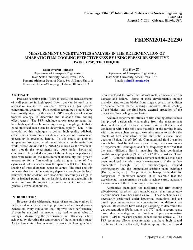
A pressure and temperature-controlled cell was used to calibrate the PSP, as in the diagram in Fig. 1(a). The calibration cell, seen in Fig. 1(b), contains two chambers separated by a


copper test plate. The front of the test plate was painted with PSP while the back of the test plate was exposed to an enclosed chamber through which coolant fluid was circulated. An external thermal regulator was used to circulate and control the temperature of the coolant. The frontal chamber has a silicon-quartz window through which the test plate was illuminated and imaged. This chamber is pressure-controlled and the pressure within the chamber was measured with a digital pressure transducer [DSA 3217 Module, Scanivalve Corp, 100 psi full scale with ±0.05 psi accuracy]. A K-type thermocouple and reader with 0.1˚C resolution continuously monitored the temperature of this chamber. Because the effectiveness measurements utilize a foreign gas with zero O2 content to simulate the coolant flow, the calibration needs to be performed using vacuum pressure. A vacuum pump was employed to depressurize the cell for most of the range of the calibration while a continuous CO2-flush was used to achieve a calibration point at true-zero O2 pressure. A reference pressure of 1 atm (absolute) was used, which corresponds in the wind tunnel

experiments to a condition of η=0.

The paint that was chosen for this experimental campaign

is ISSI UniFIB due to its low stated temperature sensitivity (~0.5%/˚C) and single-coat application. The paint has peak emission intensity at 650 nm upon illumination with 390 nm UV light. Imaging of the flow is accomplished through use of a

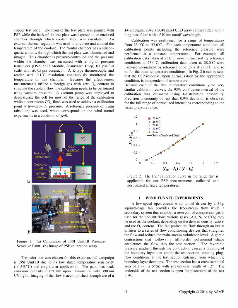
14-bit digital 2048 x 2048 pixel CCD array camera fitted with a long-pass filter with a 610 nm cutoff wavelength.

Calibration was performed for a range of temperatures from 23.0˚C to 32.6˚C. For each temperature condition, all calibration points including the reference pressure were performed at a constant temperature. For example, all calibration data taken at 23.0˚C were normalized by reference conditions at 23.0˚C, calibration data taken at 28.0˚C were likewise normalized by reference conditions at 28.0˚C, and so on for the other temperature conditions. In Fig. 2 it can be seen that the PSP response, upon normalization by the appropriate condition, is independent of temperature. Because each of the five temperature conditions yield very similar calibration curves, the 95% confidence interval of the calibration was estimated using t-distribution probability. Precision uncertainty of less than 0.9% deviation is observed for the full range of normalized intensities corresponding to the tested pressure range.

1. WIND TUNNEL EXPERIMENTS

A low-speed open-circuit wind tunnel driven by a 3 hp squirrel-cage fan provides the free-stream flow while a secondary system that employs a reservoir of compressed gas is used for the coolant flow; various gases (Air, N2 or CO2) may be used as the coolant, depending on the desired density ratio P and the O2 content. The fan pushes the flow through an initial diffuser to a series of flow conditioning devices that straighten the flow and reduce the main-stream turbulence level. A gentle contraction that follows a fifth-order polynomial shape accelerates the flow into the test section. The favorable pressure gradient through the contraction causes a thinning of the boundary layer that enters the test section, creating plug-flow conditions at the test section entrance from which the boundary layer develops. The test section has a cross-sectional area of 8”(w) x 5”(h) with stream-wise length of 12”. The underside of the test section is open for placement of the test plate.

(a)

(b)

Figure 1. (a) Calibration of ISSI UniFIB Pressure-

Sensitive Paint. (b) Image of PSP calibration setup.

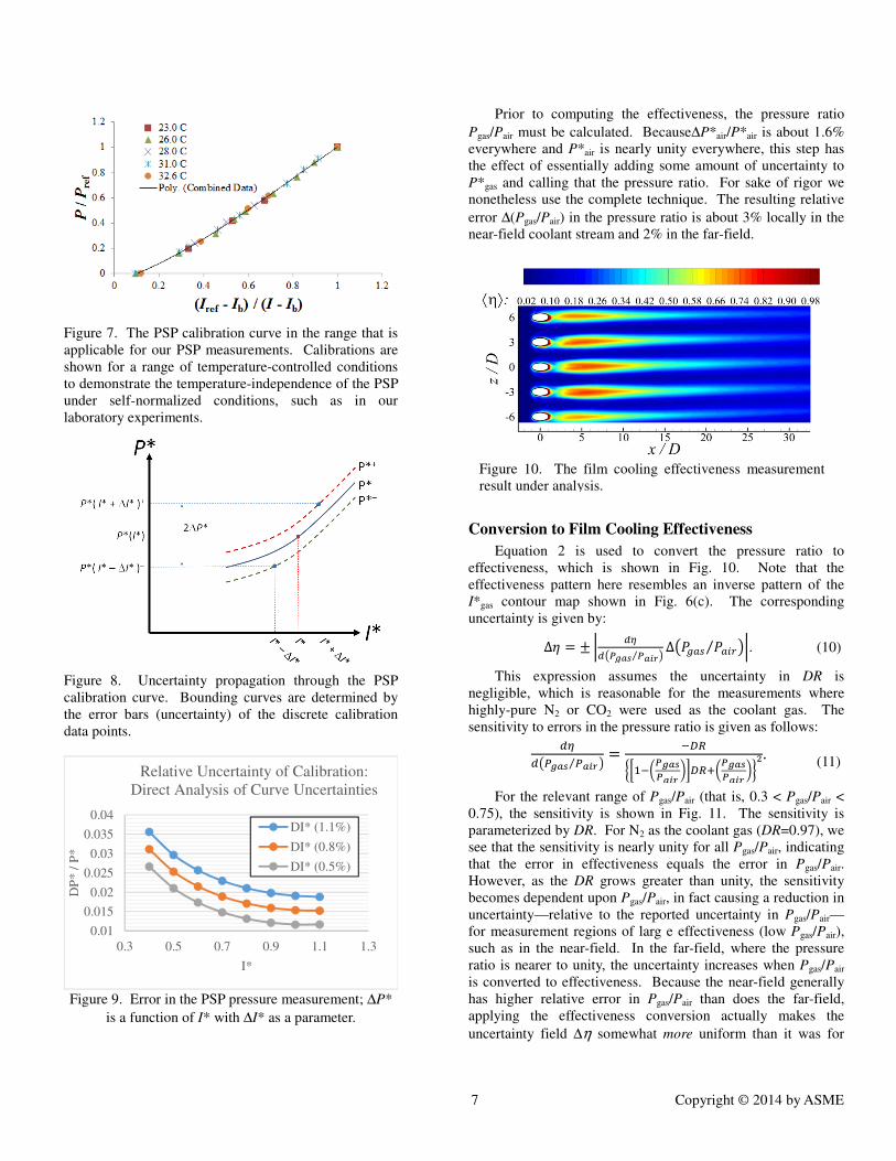
Figure 2. The PSP calibration curve in the range that is applicable for our PSP measurements, collected and

normalized at fixed temperatures.


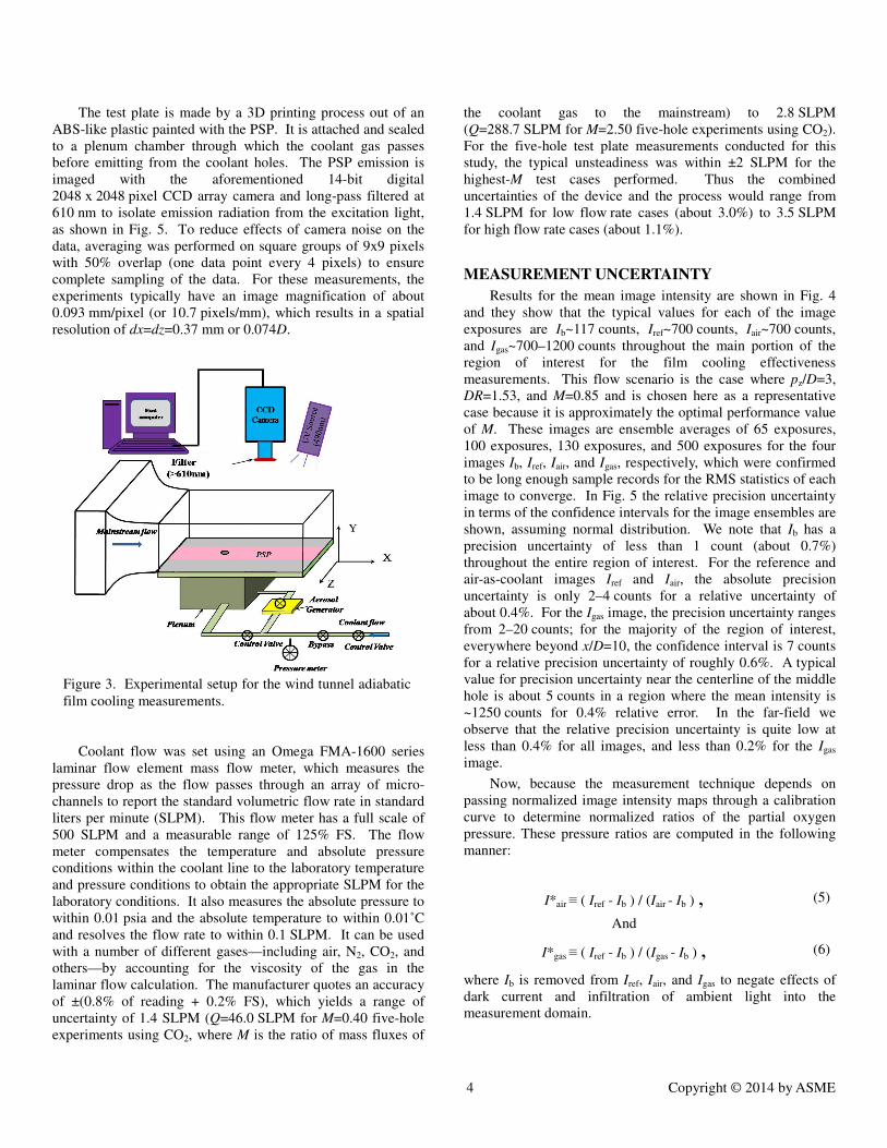
The test plate is made by a 3D printing process out of an ABS-like plastic painted with the PSP. It is attached and sealed to a plenum chamber through which the coolant gas passes before emitting from the coolant holes. The PSP emission is imaged with the aforementioned 14-bit digital 2048 x 2048 pixel CCD array camera and long-pass filtered at 610 nm to isolate emission radiation from the excitation light, as shown in Fig. 5. To reduce effects of camera noise on the data, averaging was performed on square groups of 9x9 pixels with 50% overlap (one data point every 4 pixels) to ensure complete sampling of the data. For these measurements, the experiments typically have an image magnification of about 0.093 mm/pixel (or 10.7 pixels/mm), which results in a spatial resolution of dx=dz=0.37 mm or 0.074D.

Coolant flow was set using an Omega FMA-1600 series laminar flow element mass flow meter, which measures the pressure drop as the flow passes through an array of micro-channels to report the standard volumetric flow rate in standard liters per minute (SLPM). This flow meter has a full scale of 500 SLPM and a measurable range of 125% FS. The flow meter compensates the temperature and absolute pressure conditions within the coolant line to the laboratory temperature and pressure conditions to obtain the appropriate SLPM for the laboratory conditions. It also measures the absolute pressure to within 0.01 psia and the absolute temperature to within 0.01˚C and resolves the flow rate to within 0.1 SLPM. It can be used with a number of different gases—including air, N2, CO2, and others—by accounting for the viscosity of the gas in the laminar flow calculation. The manufacturer quotes an accuracy of ±(0.8% of reading + 0.2% FS), which yields a range of uncertainty of 1.4 SLPM (Q=46.0 SLPM for M=0.40 five-hole experiments using CO2, where M is the ratio of mass fluxes of

the coolant gas to the mainstream) to 2.8 SLPM (Q=288.7 SLPM for M=2.50 five-hole experiments using CO2). For the five-hole test plate measurements conducted for this study, the typical unsteadiness was within ±2 SLPM for the highest-M test cases performed. Thus the combined uncertainties of the device and the process would range from 1.4 SLPM for low flow rate cases (about 3.0%) to 3.5 SLPM for high flow rate cases (about 1.1%).

MEASUREMENT UNCERTAINTY

Results for the mean image intensity are shown in Fig. 4 and they show that the typical values for each of the image exposures are Ib~117 counts, Iref~700 counts, Iair~700 counts, and Igas~700–1200 counts throughout the main portion of the region of interest for the film cooling effectiveness measurements. This flow scenario is the case where pz/D=3, DR=1.53, and M=0.85 and is chosen here as a representative case because it is approximately the optimal performance value of M. These images are ensemble averages of 65 exposures, 100 exposures, 130 exposures, and 500 exposures for the four images Ib, Iref, Iair, and Igas, respectively, which were confirmed to be long enough sample records for the RMS statistics of each image to converge. In Fig. 5 the relative precision uncertainty in terms of the confidence intervals for the image ensembles are shown, assuming normal distribution. We note that Ib has a precision uncertainty of less than 1 count (about 0.7%) throughout the entire region of interest. For the reference and air-as-coolant images Iref and Iair, the absolute precision uncertainty is only 2–4 counts for a relative uncertainty of about 0.4%. For the Igas image, the precision uncertainty ranges from 2–20 counts; for the majority of the region of interest, everywhere beyond x/D=10, the confidence interval is 7 counts for a relative precision uncertainty of roughly 0.6%. A typical value for precision uncertainty near the centerline of the middle hole is about 5 counts in a region where the mean intensity is ~1250 counts for 0.4% relative error. In the far-field we observe that the relative precision uncertainty is quite low at less than 0.4% for all images, and less than 0.2% for the Igas image.

Now, because the measurement technique depends on passing normalized image intensity maps through a calibration curve to determine normalized ratios of the partial oxygen pressure. These pressure ratios are computed in the following manner:

I*air ≡ ( Iref - Ib ) / (Iair - Ib ) , (5)

And

I*gas ≡ ( Iref - Ib ) / (Igas - Ib ) , (6)

where Ib is removed from Iref, Iair, and Igas to negate effects of dark current and infiltration of ambient light into the measurement domain.

Figure 3. Experimental setup for the wind tunnel adiabatic

film cooling measurements.


It is necessary to compute the uncertainties of the image

intensity ratios I*air and I*gas, ∆I*air and ∆I*gas, respectively. The appropriate expressions for the uncertainties of these intensity ratios are:

#��∗��∗ = $%#��#�� &' + �#��#�� '

, (7)

#��∗��∗ = $%#��#�� &' + %#��#�� &'

, (8)

where the numerators and denominators of I*air and I*gas are each treated distinctly to arrive at the two terms under the radicals. It should be noted here that bias error in the individual images is expected to cancel out during the image normalization operation, and that only the precision uncertainty of the four images propagates into the uncertainty of the intensity ratios. In Fig. 6 we see the computed intensity ratios and their relative uncertainties. The intensity ratio I*air is nearly unity throughout the entire painted measurement domain. In the near field, it has a value of roughly 1.02 and a value of 1.00 elsewhere in the region of interest. Therefore, the absolute and relative uncertainty are valued approximately identically at about ±0.02, or ±2%. The other intensity ratio I*gas ranges from 0.44 to 1.00 in the region of interest with a relative uncertainty of ±2% in isolated local regions in the near-field of the coolant streams and ±0.5% throughout the far field. Near-centerline values of the relative uncertainty near the middle hole are about ±2%. The corresponding absolute uncertainty values range from ±0.009 to ±0.01 throughout the region of interest.

PSP CALIBRATION UNCERTAINTY

The next step in the measurement process is to convert the intensity ratios to normalized oxygen pressure ratios through use of a calibration, which is shown in Fig. 7. The calibration was performed for five different temperature conditions that were later used to determine the precision uncertainty of the calibration curve, which came to about 0.9% or less, showing that the PSP is quite insensitive to temperature effects provided the images are normalized with a reference image taken at the same temperature, as they were for these calibration runs.

An additional check of the calibration uncertainty was performed whereby error bars of pressure and image intensity were determined for each calibration data point. The calibration data [(I*)i, (P*)i] were then plotted and a calibration curve fit to them. Additionally, calibration curves P*– and P*+

were also fit to the limiting extents of the error bars [(I*+∆I*)i,

(P*-∆P*)] and [(I*-∆I*)i, (P*+∆P*)], respectively. From there, the calibration curve was analyzed in the manner demonstrated in Fig. 8, where the range in variation of uncertainty in P* is determined as:

Δ*∗ = �' +*∗��∗ − Δ�∗" − *∗��∗ + Δ�∗",. (9)

The end result of this analysis is a lookup table for

measurement uncertainty where by ∆P*/P* is found as a

function of I* with ∆I* as a parameter, as shown in Fig. 9. The relative uncertainty in P* reaches as high as 3.6% at low I*

values where ∆I* is high, such as in the near-field edge regions of certain coolant streams.

(a)

(b)

(c)

(d) Figure 4. Mean intensity maps of the four ensemble-averaged image emission intensity maps. Units are in terms of image intensity counts, which is a multiple of electrons freed by photons incident upon the CCD array.

(a) Ib, (b) Iref, (c) Iair, (d) Igas.


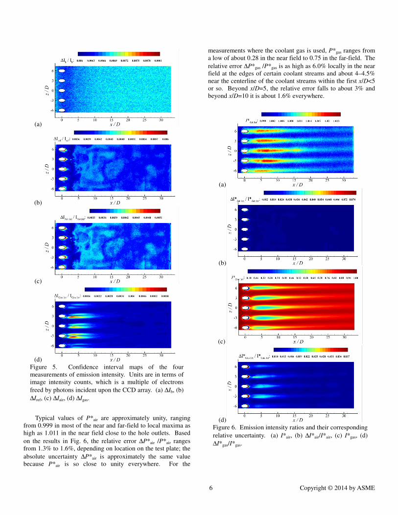
Typical values of P*air are approximately unity, ranging from 0.999 in most of the near and far-field to local maxima as high as 1.011 in the near field close to the hole outlets. Based

on the results in Fig. 6, the relative error ∆P*air /P*air ranges from 1.3% to 1.6%, depending on location on the test plate; the

absolute uncertainty ∆P*air is approximately the same value because P*air is so close to unity everywhere. For the

measurements where the coolant gas is used, P*gas ranges from a low of about 0.28 in the near field to 0.75 in the far-field. The

relative error ∆P*gas /P*gas is as high as 6.0% locally in the near field at the edges of certain coolant streams and about 4–4.5% near the centerline of the coolant streams within the first x/D<5 or so. Beyond x/D=5, the relative error falls to about 3% and beyond x/D=10 it is about 1.6% everywhere.

(a)

(b)

(c)

(d) Figure 5. Confidence interval maps of the four measurements of emission intensity. Units are in terms of image intensity counts, which is a multiple of electrons

freed by photons incident upon the CCD array. (a) ∆Ib, (b)

∆Iref, (c) ∆Iair, (d) ∆Igas.

(a)

(b)

(c)

(d) Figure 6. Emission intensity ratios and their corresponding

relative uncertainty. (a) I*air, (b) ∆I*air/I*air, (c) I*gas, (d)

∆I*gas/I*gas.


Prior to computing the effectiveness, the pressure ratio

Pgas/Pair must be calculated. Because∆P*air/P*air is about 1.6% everywhere and P*air is nearly unity everywhere, this step has the effect of essentially adding some amount of uncertainty to P*gas and calling that the pressure ratio. For sake of rigor we nonetheless use the complete technique. The resulting relative

error ∆(Pgas/Pair) in the pressure ratio is about 3% locally in the near-field coolant stream and 2% in the far-field.

Conversion to Film Cooling Effectiveness

Equation 2 is used to convert the pressure ratio to effectiveness, which is shown in Fig. 10. Note that the effectiveness pattern here resembles an inverse pattern of the I*gas contour map shown in Fig. 6(c). The corresponding uncertainty is given by:

Δ� = ± . /0/1�� ⁄ 2 Δ1*345 *4 6⁄ 2.. (10)

This expression assumes the uncertainty in DR is negligible, which is reasonable for the measurements where highly-pure N2 or CO2 were used as the coolant gas. The sensitivity to errors in the pressure ratio is given as follows:

/0/1�� ⁄ 2 = ��

78��%9��9� &:��%9��9� &;<. (11)

For the relevant range of Pgas/Pair (that is, 0.3 < Pgas/Pair < 0.75), the sensitivity is shown in Fig. 11. The sensitivity is parameterized by DR. For N2 as the coolant gas (DR=0.97), we see that the sensitivity is nearly unity for all Pgas/Pair, indicating that the error in effectiveness equals the error in Pgas/Pair. However, as the DR grows greater than unity, the sensitivity becomes dependent upon Pgas/Pair, in fact causing a reduction in uncertainty—relative to the reported uncertainty in Pgas/Pair—for measurement regions of larg e effectiveness (low Pgas/Pair), such as in the near-field. In the far-field, where the pressure ratio is nearer to unity, the uncertainty increases when Pgas/Pair is converted to effectiveness. Because the near-field generally has higher relative error in Pgas/Pair than does the far-field, applying the effectiveness conversion actually makes the

uncertainty field ∆η somewhat more uniform than it was for

Figure 7. The PSP calibration curve in the range that is applicable for our PSP measurements. Calibrations are shown for a range of temperature-controlled conditions to demonstrate the temperature-independence of the PSP under self-normalized conditions, such as in our laboratory experiments.

Figure 8. Uncertainty propagation through the PSP calibration curve. Bounding curves are determined by the error bars (uncertainty) of the discrete calibration data points.

Figure 9. Error in the PSP pressure measurement; ∆P*

is a function of I* with ∆I* as a parameter.

0.01

0.015

0.02

0.025

0.03

0.035

0.04

0.3 0.5 0.7 0.9 1.1 1.3

DP

* /

P*

I*

Relative Uncertainty of Calibration:Direct Analysis of Curve Uncertainties

DI* (1.1%)

DI* (0.8%)

DI* (0.5%)

Figure 10. The film cooling effectiveness measurement result under analysis.


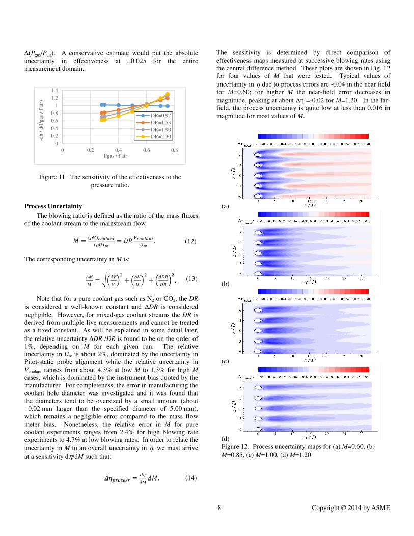
∆(Pgas/Pair). A conservative estimate would put the absolute uncertainty in effectiveness at ±0.025 for the entire measurement domain.

Process Uncertainty

The blowing ratio is defined as the ratio of the mass fluxes of the coolant stream to the mainstream flow.

= = �>?"@AABC��>D"E = FG ?@AABC�DE . (12)

The corresponding uncertainty in M is:

#HH = I�#?? �' + �#DD �' + �#�� '. (13)

Note that for a pure coolant gas such as N2 or CO2, the DR

is considered a well-known constant and ∆DR is considered negligible. However, for mixed-gas coolant streams the DR is derived from multiple live measurements and cannot be treated as a fixed constant. As will be explained in some detail later,

the relative uncertainty ∆DR /DR is found to be on the order of 1%, depending on M for each given run. The relative uncertainty in U∞ is about 2%, dominated by the uncertainty in Pitot-static probe alignment while the relative uncertainty in Vcoolant ranges from about 4.3% at low M to 1.3% for high M cases, which is dominated by the instrument bias quoted by the manufacturer. For completeness, the error in manufacturing the coolant hole diameter was investigated and it was found that the diameters tend to be oversized by a small amount (about +0.02 mm larger than the specified diameter of 5.00 mm), which remains a negligible error compared to the mass flow meter bias. Nonetheless, the relative error in M for pure coolant experiments ranges from 2.4% for high blowing rate experiments to 4.7% at low blowing rates. In order to relate the

uncertainty in M to an overall uncertainty in η, we must arrive

at a sensitivity dη/dM such that:

J�K6LMN55 = O0OH J=. (14)

The sensitivity is determined by direct comparison of effectiveness maps measured at successive blowing rates using the central difference method. These plots are shown in Fig. 12 for four values of M that were tested. Typical values of

uncertainty in η due to process errors are -0.04 in the near field for M=0.60; for higher M the near-field error decreases in

magnitude, peaking at about ∆η =-0.02 for M=1.20. In the far-field, the process uncertainty is quite low at less than 0.016 in magnitude for most values of M.

Figure 11. The sensitivity of the effectiveness to the

pressure ratio.

0

0.2

0.4

0.6

0.8

1

1.2

1.4

0 0.2 0.4 0.6 0.8

-dh

/ d

(Pgas

/ P

air)

Pgas / Pair

DR=0.97

DR=1.53

DR=1.90

DR=2.30

(a)

(b)

(c)

(d) Figure 12. Process uncertainty maps for (a) M=0.60, (b)

M=0.85, (c) M=1.00, (d) M=1.20


CONCLUSIONS

For the particular flow scenario in question, the PSP film cooling effectiveness measurement technique has a varying degree of certainty throughout the measurement domain. The combination of the measurement (bias) uncertainty and the precision uncertainty through the root-sum-square method gives the total uncertainty. Based on the estimates of uncertainty made so far, a fair estimate for the near-field

absolute uncertainty is about ∆ηtotal=±0.047 in the near field, or approximately %. Similarly, a fair estimate for the far-field

absolute uncertainty is ∆ηtotal=±0.032. In the near-field, where the coolant stream has freshly emitted from the plenum, there are regions of high fluctuation in the flow that cause a total uncertainty perhaps as high as 5% in certain locations. Comparatively, the total uncertainty in the far-field is significantly lower at 3%. The flow field in this region is characterized by weaker fluctuations than near the coolant holes and in that same spirit the PSP output is generally much steadier in this region, which allows a more reliable measurement in the far field than the near. Thus it would seem that this technique is somewhat better-suited for absolute effectiveness measurements in regions of stable flow. For comparison, the TSP technique carried out by Kunze, et al (2008) quotes uncertainties on the order of 4% for η = 0.8 and 10 % for η = 0.3. A comparison to the uncertainties of other methods would be of some use (IR thermography, TSP, etc), with citations to some representative papers regarding those methods.

ACKNOWLEDGMENTS The technical assistance of Dr. Wontae Hwang of GE

Global Research Center in Niskayuna, New York is greatly appreciated. Special thanks go to Mr. Bill Rickard, Mr. Andrew Jordan, and Mr. Jim Benson for their technical support and expertise throughout this study. Grateful acknowledgements also go to Mr. Marc Regan, Mr. Mark Johnson, and Mr. Omar Longuo for their assistance with setup and conduction of these experiments.

REFERENCES

Baldauf, S., Schulz, A, and Wittig, S. 2001. “High-Resolution Measurements of Local Effectiveness from Discrete Hole Film Cooling.” Journal of Turbomachinery. Vol. 123, pp. 758–765.

Charbonnier, D., Ott, P., Jonsson, M., Cottier, F., and Kobke, Th. 2009. “Experimental and Numerical Study of the Thermal Performance of a Film Cooled Turbine Platform.” Proc. Of ASME Turbo Expo 2009: Power for Land, Sea and Air. June 8–12, 2009.

Dhungel, A., Lu, Y., Phillips, W., Ekkad, S.V., Heidmann, J. 2009. “Film Cooling from a Row of Holes Supplemented with Antivortex Holes.” Journal of Turbomachinery. Vol. 131, pp. 021007-1–10

Goldstein, R. J., E. R. G. Eckert, and F. Burggraf. "Effects of hole geometry and density on three-dimensional film

cooling." International Journal of Heat and Mass

Transfer 17.5 (1974): 595-607.

Hammer, M., Norris, J., and Lafferty, J.F. 2004. “Recent Developments in TSP/PSP Technologies Focusing on High Velocity-Temperature and Non-Oxygen Environments.” 24th AIAA Aerodynamic Measurement Technology and Ground Testing Conference, June 28–July 1, 2004, Portland, Oregon.

Heidmann, J.D. and Ekkad, S. 2008. “A Novel Antivortex Turbine Film-Cooling Hole Concept.” Journal of Turbomachinery. Vol. 130, pp. 031020-1–9.

Jones, T.V. 1999. “Theory for the Use of Foreign Gas in Simulating Film Cooling.” International Journal of Heat and Fluid Flow. Vol. 20, pp. 349–354.

Kline, S. J., & McClintock, F. A. (1953). Describing uncertainties in single-sample experiments. Mechanical

engineering, 75(1), 3-8.

Knost, D. G., & Thole, K. A. 2003. “Computational predictions of endwall film-cooling for a first stage vane.” In ASME

Turbo Expo 2003, collocated with the 2003 International

Joint Power Generation Conference (pp. 163-173). American Society of Mechanical Engineers.

Kunze, M., Preibisch, S., Vogeler, K., Landis, K., & Heselhaus, A. (2008, January). A new test rig for film cooling experiments on turbine endwalls. InASME Turbo Expo 2008: Power for Land, Sea, and Air (pp. 989-998). American Society of Mechanical Engineers.

Leylek, J. H., and Zerkle, R. D., 1994, “Discrete-Jet Film Cooling: A Comparison of Computational Results With Experiments,” ASME J. Turbomach., 116, pp. 358–368.Ligrani, et al (1994a)

Pedersen, D. R., Eckert, E. R. G., and Goldstein, R. J., 1977, ‘‘Film Cooling With Large Density Differences Between the Mainstream and the Secondary Fluid Measured by the Heat–Mass Transfer Analogy,’’ASME J. Heat Transfer, 99, pp. 620–627.

Rallabandi, A.P., Grizzle, J., Han, J-C. 2011. “Effect of Upstream Step on Flat Plate Film-Cooling Effectiveness Using PSP.” Journal of Turbomachinery. Vol. 133, pp. 041024-1–8.

Silieti, M., Kassab, A. J., & Divo, E., 2009, “Film cooling effectiveness: Comparison of adiabatic and conjugate heat transfer CFD models.” International Journal of Thermal

Sciences, 48(12), 2237-2248.

Wright, Lesley M., Stephen T. McClain, and Michael D. Clemenson. "Effect of density ratio on flat plate film cooling with shaped holes using PSP." Journal of

turbomachinery 133.4 (2011).

Wright, Lesley M., Stephen T. McClain, and Michael D. Clemenson. "PIV Investigation of the Effect of Freestream Turbulence Intensity on Film Cooling from Fanshaped Holes." ASME, 2011.

Yang, Z. and Hu, H. 2011. “A Study of Trailing-Edge Cooling Using Pressure Sensitive Paint Technique.” Journal of Propulsion and Power. Vol. 27, No. 3, pp. 700–709.

Documents

2014-ASME-FED-PSP Uncertainty-final-out-xx