Embed Size (px)
Citation preview

Sarosh H. Lodi Aslam F. Mohammed Rashid A. Khan NED University of Engineering and Technology
M. Selim Gunay University of California, Berkeley
Supported by the Pakistan‐US Science and Technology Cooperation Program
of Reinforced Concrete Buildings with Masonry Infill Walls
A Practical Guide to Nonlinear Static Analysis


A Practical Guide to Nonlinear Static Analysis
Preface
Reinforced concrete (RC) frames with unreinforced masonry (URM) infill walls are commonly used as the structural system for buildings in many seismically active regions around the world. Structural engineers recognize that many buildings of this type have performed poorly during earthquakes. URM infill walls used in Pakistan and adjoining regions comprise of either burnt clay bricks or cement concrete block masonry. These URM infill walls are generally treated as non-structural elements, because they are used mainly for architectural purposes, and structural engineers often ignore them during structural design.
During earthquakes, infill walls affect the response of the structure, and may either beneficial or detrimental effects. Infill walls contribute to the lateral force resisting capacity and damping of the structure up to a certain level of ground motion. Infill walls increase the initial stiffness and decrease the fundamental period of the structure, which might be beneficial or detrimental, depending on the frequency content of the ground motion.
URM infill walls are prone to early brittle failure, and infill wall failures may lead to the formation of a weak story, which can cause the building to collapse. Infill walls interact with the surrounding frame in such a way that column shear failure is made more likely. In addition, an unequal spatial distribution of infill walls for functional reasons – for example, windows and open commercial spaces on the street frontage and full walls adjacent to neighbouring buildings – can create torsion that places additional demands on columns and may cause them to fail.
Because of the potentially dire consequences of ignoring the structural role of URM infill walls, proper consideration of infill walls is essential in any structural analysis of RC frame buildings with infill walls. This document provides engineers with guidance on how to model infill walls and include them in structural analyses. Because the consequences of ignoring infill walls are not region related but exist throughout the world, the authors anticipate that the guide will be useful for practicing engineers in Pakistan as well as in other countries with many similar buildings.
This document discusses and illustrates how to analyze infill building with an example in ETABS© building analysis and design software by Computers and Structures, Inc. of a 2-D nonlinear static “pushover” analysis of a six storey RC building with URM infill walls, based on guidelines and modeling procedures given in the ATC-40 and FEMA-356 documents. The procedures for defining the strength and stiffness of equivalent strut members used to model infill walls are also applicable for linear analyses.
This manual was developed as part of a project that NED University of Engineering (NED) and Technology and GeoHazards International (GHI), a California based non-profit organization that improves global earthquake safety, conducted together to assess and design seismic retrofits for existing buildings typical of the local building stock, such as the one described in this report. The project was funded by the Pakistan Higher Education Commission (HEC) and The National Academies through a grant from the United States Agency for International Development (USAID).
3

A Practical Guide to Nonlinear Static Analysis of Reinforced Concrete Buildings with Masonry Infill Walls
Copyright 2011 NED University of Engineering and Technology, and GeoHazards International. All rights reserved, with the exception that Computers and Structures, Inc. retains copyright to all material pertaining to their ETABS© building analysis and design software.
Developed by: Sarosh H. Lodi, Professor and Dean, Faculty of Civil Engineering and Architecture, NED University of Engineering and Technology, Karachi Aslam F. Mohammed, Assistant Professor, NED University of Engineering and Technology, Karachi Rashid A. Khan, Professor, NED University of Engineering and Technology, Karachi M. Selim Gunay, Post-doctoral Researcher, University of California, Berkeley Technical reviewers: Khalid M. Mosalam, Professor, University of California, Berkeley Gregory G. Deierlein, Professor, Stanford University David Mar, Principal, Tipping Mar, Berkeley California Sahibzada F. A. Rafeeqi, Professor and Pro-Vice Chancellor, NED University of Engineering and Technology, Karachi Technical editing: Janise Rodgers, GeoHazards International Justin Moresco, GeoHazards International
Acknowledgments: The project team wishes to thank Computers and Structures, Inc. of Berkeley, California for their generous donation of ETABS© building analysis and design software, which was used to perform the analyses in this guide.
Disclaimer: All parties, including but not limited to NED University of Engineering and Technology, GeoHazards International, Higher Education Commission, The National Academies, the United States Agency for International Development, and Computers and Structures, Inc., are not responsible for any damage or harm that may occur despite or because of the application of measures and techniques described in this guide. In addition, users of this guide are solely responsible for the accuracy of structural models, analyses, and results and for their subsequent usage in any structural design or construction works.

A Practical Guide to Nonlinear Static Analysis
Contents
Chapter 1 Introduction..........................................................................................................7 Chapter 2 Masonry Infill Walls are Important .....................................................................8
An Example of the Effects of Unreinforced Masonry Infill ................................................10 Chapter 3 Performance Based Analysis .............................................................................12
3.1 Nonlinear Static Procedures in Current Standards.........................................................12 3.1.1 Displacement Coefficient Method from FEMA 356 / ASCE 41...........................13 3.1.2 Capacity Spectrum Method from ATC-40 ............................................................14
3.2 Modelling Infill Walls as Struts....................................................................................15 Chapter 4 Pushover Analysis Using ETABS .....................................................................18
4.1 Defining how nonlinearity is considered .....................................................................18 4.2 Determining Analysis Cases ........................................................................................19 4.3 Defining Loading .........................................................................................................19 4.4 Selecting the Type of Load Control.............................................................................20 4.5 Analysis Results...........................................................................................................20 4.6 Procedure .....................................................................................................................21 4.7 Important Considerations.............................................................................................21
Chapter 5 Example of Pushover Analysis Using ETABS .......................................................22 5.1 Modelling.....................................................................................................................22 5.2 Defining and Assigning Loads on Structure .............................................................30 5.3 Analysis.....................................................................................................................34
5.3.2 Non-Linear Static Analysis................................................................................36 5.4 Results .......................................................................................................................53
Sources of Additional Information ..........................................................................................58 References................................................................................................................................59
5


A Practical Guide to Nonlinear Static Analysis
Chapter1 Introduction
The 2005 Kashmir earthquake dramatically demonstrated the lethal combination of vulnerable buildings and strong ground shaking. But the earthquake-affected areas aren’t the only places at risk – earthquake faults underlie many parts of Pakistan. The country’s cities, including Karachi (see sidebar) have many reinforced concrete (RC) frame buildings with masonry infill walls that are at risk of earthquake damage. There is a growing need for engineers to evaluate these buildings to determine their potential performance in a major earthquake. This guide will show you how to use a simple yet powerful analysis technique called nonlinear static analysis, or pushover analysis, to determine what type and extent of earthquake damage may occur in these buildings, and the effects of potential strengthening measures that you can apply to reduce damage.
The recent advent of structural design for a particular level of earthquake performance, such as immediate post-earthquake occupancy, (termed performance based earthquake engineering), has resulted in guidelines such as ATC-40 (1996), FEMA-273 (1996) and FEMA-356 (2000) and standards such as ASCE-41 (2006), among others. New Zealand’s building code is performance-based. Among the different types of analyses described in these documents, pushover analysis comes forward because of its optimal accuracy, efficiency and ease of use.
Pushover analysis gives necessary insight into nonlinear behaviour without the additional complexities of nonlinear dynamic analysis. Pushover analysis is a static, nonlinear procedure in which the magnitude of the structural loading is incrementally increased in accordance with a certain predefined pattern. As the load increases, the structure begins to yield and become damaged, and the structural deficiencies and failure modes of the building become
apparent. The loading is monotonic (i.e., in a single direction) with the effects of the load reversals that occur during a real earthquake being estimated by using modified monotonic force-deformation criteria and with damping approximations. The goal of static pushover analysis is to evaluate the real strength of the existing structure, rather than to give the lower bound strength for design.
The city of Karachi, with more than 14 million inhabitants, sits close to a tectonic plate boundary and within reach of earthquakes on numerous faults surrounding the city. Karachi’s buildings are at risk due to the combination of seismic hazard and structural vulnerability.
Due to the reasons mentioned above, this document focuses on nonlinear static analysis with an emphasis on RC frame buildings with masonry infill walls. Pushover analysis is demonstrated using the computer software ETABS, which was developed by Berkeley, California-based Computers and Structures Inc. and is one of several available software programs with the capability to conduct pushover analysis. ETABS is an integrated building
7
analysis and design software that incorporates linear, nonlinear, static and dynamic analysis capabilities with the building design features.
Chapter2MasonryInfillWallsareImportant
Reinforced concrete (RC) frame buildings with unreinforced masonry (URM) infill walls are commonly built throughout the world, including in seismically active regions. URM infill walls are widely used as partitions throughout Pakistan, and despite often being considered as non-structural elements, they affect both the structural and non-structural performance of RC buildings. Structural engineers recognize that many buildings of this type have performed poorly and have even collapsed during recent earthquakes in Turkey, Taiwan, India, Algeria, Pakistan, China, Italy and Haiti, as Figure 1shows.
a) b)
d) c)
f) e)

A Practical Guide to Nonlinear Static Analysis
Figure 1. Masonry infill-related damage in recent earthquakes
9
However, contrary to the experience gathered from these earthquakes, these buildings continue to be built in many seismic regions around the world. Particularly in countries with emerging economies, vulnerable infilled frame buildings continue to be built at a rapid rate in order to keep up with urban population growth and contribute greatly to increased global earthquake risk. When the seismic vulnerabilities present in the RC system (such as lack of confinement at the beam and column ends and the beam column joints, strong beam-weak column proportions, and presence of shear-critical columns) are combined with the complexity due to the interaction of the infill walls and the surrounding frame and the brittleness of the URM materials, non-ductile RC frames with URM infill walls may be considered as one of the world’s most common types of seismically vulnerable buildings. Therefore, it is essential to apply existing knowledge on the behaviour of this complex structural system to develop proper modelling techniques and adequate retrofit methods.
URM infill walls are generally treated as non-structural elements which are used mainly for architectural purposes. However, many researchers (e.g., Humar et al., 2001; Saatcioglu et al., 2001; Korkmaz et al., 2007; Mondal and Jain, 2008; Taher, et al., 2008) and the experiences in past earthquakes have shown that the presence of URM walls changes the seismic response of framed building. The URM walls function as structural elements, and they may have beneficial or detrimental effects. Infill walls contribute to the lateral force resisting capacity and damping of the structure up to a certain level of structural response. They increase the initial stiffness and decrease the initial period of the structure, which might be beneficial or detrimental depending on the frequency content of the experienced ground motion. URM infill walls are prone to early brittle failure. Infill walls interacting with frames tend to alter the building’s overall strength and stiffness distribution. This may be despite the design intent of the engineer, because infill walls are typically considered as “non-structural” and therefore neglected in the frame design. Many buildings have a soft storey created by commercial space (shops) or parking at the ground floor (Figure 1a and b). Even in buildings without open spaces at the ground floor, brittle infill wall failure may lead to the formation of a weak and soft storey during ground shaking in buildings that would have otherwise not had one (Figure 1c and d). In addition, infill walls interact with the surrounding frame in such a way that column shear failure is made more likely (Figure 1e). Infill walls can also induce torsion when some sides of the building have solid infill walls and the other sides have either infill walls with openings or no infill walls for architectural or usage purposes (Figure 1f).
Most of the damage to reinforced concrete buildings observed after the 2005 Kashmir earthquake was attributed to poor material quality, inadequate reinforcement details and poor construction practices. Many URM infill walls were damaged themselves, and led to soft storey collapses in medium to high rise buildings with commercial space (shops) or parking at the ground floor and a large concentration of heavy, stiff infill walls in the stories above. These vulnerabilities in RC buildings exist throughout Pakistan.
Considering the severity of the detrimental effects of infill – they can cause collapse – proper modelling of URM infill walls within RC frames is essential for seismic evaluation and consequently for the selection of adequate retrofit solutions to reduce damage and its consequences.
AnExampleoftheEffectsofUnreinforcedMasonryInfill
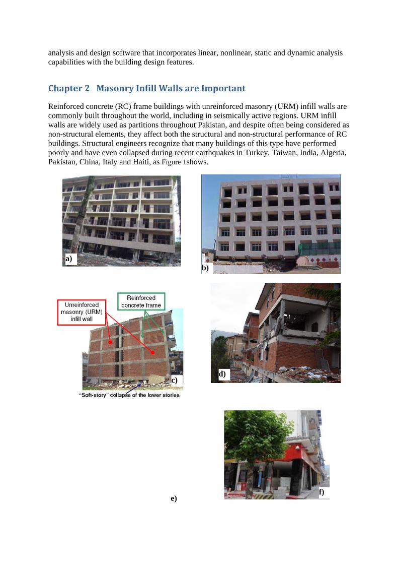
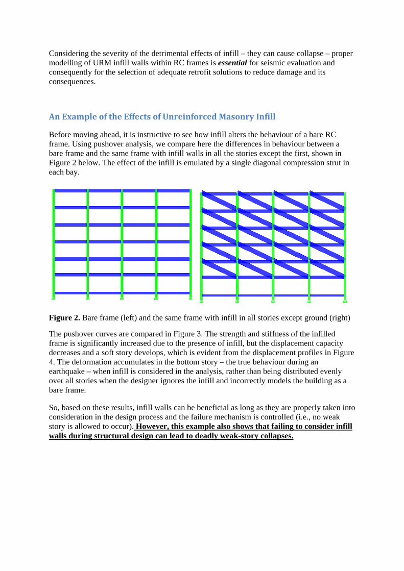
Before moving ahead, it is instructive to see how infill alters the behaviour of a bare RC frame. Using pushover analysis, we compare here the differences in behaviour between a bare frame and the same frame with infill walls in all the stories except the first, shown in Figure 2 below. The effect of the infill is emulated by a single diagonal compression strut in each bay.
Figure 2. Bare frame (left) and the same frame with infill in all stories except ground (right)
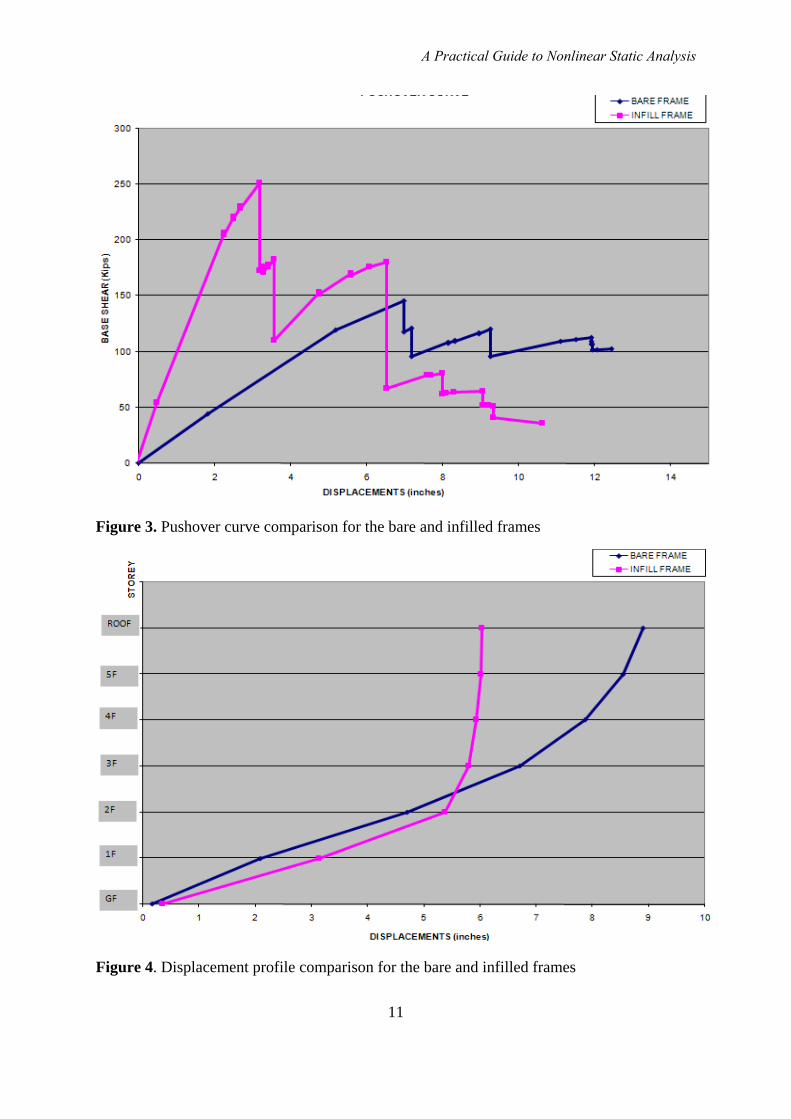
The pushover curves are compared in Figure 3. The strength and stiffness of the infilled frame is significantly increased due to the presence of infill, but the displacement capacity decreases and a soft story develops, which is evident from the displacement profiles in Figure 4. The deformation accumulates in the bottom story – the true behaviour during an earthquake – when infill is considered in the analysis, rather than being distributed evenly over all stories when the designer ignores the infill and incorrectly models the building as a bare frame.
So, based on these results, infill walls can be beneficial as long as they are properly taken into consideration in the design process and the failure mechanism is controlled (i.e., no weak story is allowed to occur). However, this example also shows that failing to consider infill walls during structural design can lead to deadly weak-story collapses.
A Practical Guide to Nonlinear Static Analysis
Figure 3. Pushover curve comparison for the bare and infilled frames
Figure 4. Displacement profile comparison for the bare and infilled frames
11

Chapter3 PerformanceBasedAnalysis
The guidelines and standards mentioned in the introduction include modelling procedures, acceptance criteria and analysis procedures for pushover analysis. These documents define force-deformation criteria for potential locations of lumped inelastic behaviour, designated as plastic hinges used in pushover analysis. As shown in Figure 5 below, five points labelled A, B, C, D, and E are used to define the force deformation behaviour of the plastic hinge, and three points labelled IO (Immediate Occupancy), LS (Life Safety) and CP (Collapse Prevention) are used to define the acceptance criteria for the hinge. In these documents, if all the members meet the acceptance criteria for a particular performance level, such as Life Safety, then the entire structure is expected to achieve the Life Safety level of performance. The values assigned to each of these points vary depending on the type of member as well as many other parameters, such as the expected type of failure, the level of stresses with respect to the strength, or code compliance.
Figure 5. Force-Deformation Relation for Plastic Hinge in Pushover Analysis
Both the ATC-40 and FEMA 356 documents present similar performance-based engineering methods that rely on nonlinear static analysis procedures for prediction of structural demands. While procedures in both documents involve generation of a “pushover” curve to predict the inelastic force-deformation behaviour of the structure, they differ in the technique used to calculate the global inelastic displacement demand for a given ground motion. The FEMA 356 document uses the Coefficient Method, whereby displacement demand is calculated by modifying elastic predictions of displacement demand. The ATC-40 Report details the Capacity-Spectrum Method, whereby modal displacement demand is determined from the intersection of a capacity curve, derived from the pushover curve, with a demand curve that consists of the smoothed response spectrum representing the design ground motion, modified to account for hysteretic damping effects.
3.1NonlinearStaticProceduresinCurrentStandards
Current standards such as ASCE 41 provide two alternate methods of estimating the peak displacement demand for use in nonlinear static procedures: the displacement coefficient method and the capacity spectrum method. Both methods rely on an equivalent linearization approach. The basic assumption in equivalent linearization techniques is that the maximum inelastic deformation of a nonlinear single degree of freedom (SDOF) system is approximately equal to the maximum deformation of a linear elastic SDOF system, provided
A Practical Guide to Nonlinear Static Analysis
that the linear elastic system has a period and a damping ratio that are larger than the initial values of those for the nonlinear system.
The displacement coefficient method is conceptually simpler and easier to use, and is not prone to the graphical misinterpretations that can occur with the capacity spectrum method. The authors recommend using the displacement coefficient method, either alone or to check results obtained by using the automated capacity spectrum method capabilities in ETABS.
3.1.1DisplacementCoefficientMethodfromFEMA356/ASCE41
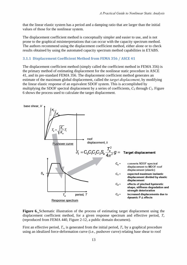
The displacement coefficient method (simply called the coefficient method in FEMA 356) is the primary method of estimating displacement for the nonlinear static procedure in ASCE 41, and its pre-standard FEMA 356. The displacement coefficient method generates an estimate of the maximum global displacement, called the target displacement, by modifying the linear elastic response of an equivalent SDOF system. This is accomplished by multiplying the SDOF spectral displacement by a series of coefficients, C0 through C3. Figure 6 shows the process used to calculate the target displacement.
Figure 6. Schematic illustration of the process of estimating target displacement using the displacement coefficient method, for a given response spectrum and effective period, Te (reproduced from FEMA 440, Figure 2-12, a public domain document).
First an effective period, Te, is generated from the initial period, Ti, by a graphical procedure using an idealized force-deformation curve (i.e., pushover curve) relating base shear to roof
13

displacement, which accounts for some stiffness loss as the system begins to behave inelastically. The effective period represents the linear stiffness of the equivalent SDOF system. The effective period is used to determine the equivalent SDOF system’s spectral acceleration, Sa, using an elastic response spectrum. The procedure assumes that the damping (usually 5%) is appropriate for a structure in the elastic range.
Then, the peak elastic spectral displacement is determined from the spectral acceleration using the following equation:
aeff
d ST
S2
2
4π= (1)
The Displacement Coefficient Method then uses four coefficients to convert the peak elastic spectral displacement first to elastic displacement at the roof and then to inelastic displacement at the roof. FEMA 440, Improvement of Nonlinear Static Seismic Analysis Procedures, explains each of the coefficients C0 through C3 as follows:
The coefficient C0 is a shape factor (often taken as the first mode participation factor) that simply converts the spectral displacement to the displacement at the roof. The other coefficients each account for a separate inelastic effect. The coefficient C1 is the ratio of expected displacement for a bilinear inelastic oscillator to the displacement for a linear oscillator. C1 depends on the ratio of elastic force, calculated as the spectral acceleration multiplied by the mass, to the yield strength, the period of the SDOF system, Te and the characteristic period of the spectrum. The coefficient C2 accounts for the effect of pinching in load-deformation relationships due to degradation in stiffness and strength. Finally, the coefficient C3 adjusts for second-order geometric nonlinearity (P-Δ) effects. The coefficients are empirical and derived primarily from statistical studies of the nonlinear response-history analyses of SDOF oscillators and adjusted using engineering judgment.
3.1.2CapacitySpectrumMethodfromATC‐40
The initial step in the capacity spectrum method (as used in ATC-40) is the same as in the displacement coefficient method: generate a pushover curve for the structure. However, in the capacity spectrum method, the results are plotted in acceleration-displacement response spectrum (ADRS) format, shown in Figure 7. To plot the pushover in ADRS format (called a capacity curve), the base shear versus roof displacement relationship must be converted using the dynamic properties of the system. The ground motion acceleration response spectrum, representing the seismic demand, is also converted to ADRS format, so that the capacity curve can be plotted on the same axes as the seismic demand. It is important to note that in ADRS format, period is represented by radial lines emanating from the origin.

A Practical Guide to Nonlinear Static Analysis
Figure 7. Graphical representation of the Capacity Spectrum Method, as presented in ATC-40 (reproduced from FEMA 440, a public-domain document).
Once the pushover curve and response spectrum are plotted together in ADRS format, iteration is required to determine the maximum inelastic displacement, called the performance point. FEMA 440 explains why:
The capacity spectrum method assumes that the equivalent damping of the system is proportional to the area enclosed by the capacity curve. The equivalent period, Teq, is assumed to be the secant period at which the seismic ground motion demand, reduced for the equivalent damping, intersects the capacity curve. Since the equivalent period and damping are both a function of the displacement, the solution to determine the maximum inelastic displacement (i.e., performance point) is iterative. ATC-40 imposes limits on the equivalent damping to account for strength and stiffness degradation.
3.2ModellingInfillWallsasStruts
The most common method of modelling infill walls is to use equivalent diagonal compression struts (Figure 8).
15

Figure 8. Equivalent diagonal compression strut modelling of infill walls (reproduced from FEMA 356, a public domain document)
The axial stiffness of an equivalent strut can be calculated with Equation 2 according to Section 7.5.2 of FEMA-356.
250
1 42 .
⎟⎟⎠
⎞⎜⎜⎝
⎛=
infcolfe
infm
hIEθ)sin(tE
λ (2a)
( ) diagcol Lha 4011750 .. −⋅= λ (2b)
diag
infminf L
tEak
⋅⋅= (2c)
In these equations, Em and Efe are the elastic moduli of the infill and the frame material, respectively, tinf is the thickness of the infill wall, hcol and Icol are the height and moment of inertia of the section of the column of the surrounding frame, hinf is the height of the infill wall panel and Ldiag is the length of the diagonal strut. The strength of the compression strut is calculated with Equation 3.

A Practical Guide to Nonlinear Static Analysis
cosθfsA
N infinfcomp
⋅= (3)
In Equation 3, Ainf is the cross sectional area of the infill wall, fsinf is the shear strength of masonry and θ is the angle of the diagonal strut with the horizontal.
As a special case, it is also possible to model an infill wall retrofitted with mesh reinforcement and concrete by using two diagonal struts, one of which is a compression member and the other is a tension member. In this case, stiffness is calculated with Equation 4 and distributed equally to the struts.
( ) ( )25.0
inf
inf1 4
2sin
⎥⎥⎦
⎤
⎢⎢⎣
⎡
⋅⋅⋅θ⋅⋅+⋅
=λhIE
tEtE
colfe
ccm (4a)
( ) diagcol Lha ⋅⋅λ⋅= 1175.0 − 4.0 (4b)
( )diag
ccmL
k = infinf
tEtEa ⋅+⋅⋅ (4c)
In Equation 4, Em, Ec and Efe are the elasticity moduli of the infill, concrete used for retrofit and the frame material, respectively. The other terms in the equation are defined as follows: tf is the thickness of the infill wall, tc is the thickness of the concrete, θ is the angle of the diagonal strut with the horizontal, hcol and Icol are the height and moment of inertia of the section of the column of the surrounding frame, hinf is the height of the infill wall panel and Ldiag is the length of the diagonal strut. The strengths of compression and tension members are calculated with Equations 5 and 6, respectively.
θ⋅⋅+⋅
=cos
3.3infinf cc fAfsANcomp (5)
θ
⋅⋅=
cosinfNtens yss sLfA
(6)
In Equations 5 and 6, Ainf and Ac (in2) are the cross sectional area of the infill wall and concrete, respectively, fsinf is the shear strength of masonry, fc is concrete strength (psi), and θ is the angle of the diagonal strut with the horizontal. As is the total cross sectional area of horizontal mesh reinforcement with spacing s, fys is the strength of steel, and Linf is the wall length.
17
Chapter4 PushoverAnalysisUsingETABS
Pushover analysis is a very powerful feature offered only in the non-linear version of ETABS. In addition to performing pushover analyses for performance-based seismic design, this feature can be used to perform general static nonlinear analysis and the analysis of staged (incremental) construction. ETABS menus and documentation refer to pushover analysis as static nonlinear analysis.
Performing any nonlinear analysis takes time and requires patience. Please read the following information carefully before performing pushover analysis. Make sure to pay special attention to the Important Considerations section later in this guide. The key points for conducting pushover analysis can be summarized as follows:
1. Defining how nonlinearity is considered 2. Determining analysis cases 3. Defining loading 4. Selecting the type of load control 5. Analysis Results 6. Procedure for conducting pushover analysis 7. Important Considerations
Information in the sections 4.1 through 4.7 has been adapted for Pakistan conditions from user documentation for ETABS software, prepared by Computers and Structures, Inc.
4.1Defininghownonlinearityisconsidered
Properly modelling the nonlinear behaviour that the structure is expected to undergo is very important for obtaining credible analysis results. However, more complicated models are not necessarily more accurate. When developing a model, keep in mind that pushover analysis contains inherent simplifications regarding the dynamic behaviour of the building, and select the level of model complexity accordingly. Several types of nonlinear behaviour can be considered in a pushover analysis:
1. Material nonlinearity at discrete, user-defined hinges in frame/line elements. Plastic hinges can be assigned at any number of locations along the length of any frame element (see Frame Nonlinear Hinge Assignments to Line Objects in ETABS documentation for details), wherever yielding or other inelastic behaviour is expected. Uncoupled moment, torsion, axial force and shear hinges are available. There is also a coupled P-M2-M3 hinge that considers the interaction of axial force and bending moments at the hinge location. More than one type of hinge can exist at the same location. For example, you might assign both an M3 (moment) and a V2 (shear) hinge to the same end of a frame element. Default hinge properties are provided based on ATC-40 and FEMA-356 criteria. For reinforced concrete frame buildings, use coupled P-M hinges when modelling columns and uncoupled moment hinges for beams. Separate shear hinges are recommended. To reduce the size and complexity of the model, a number of analysts check shear forces in each member against that member’s shear capacity rather than using shear hinges.
A Practical Guide to Nonlinear Static Analysis
2. Material nonlinearity in the link elements. The available nonlinear behaviour includes gap (compression only), hook (tension only), uniaxial plasticity along any degree of freedom, and two types of base isolators (biaxial plasticity and biaxial friction/pendulum). The link damper property has no effect in a static nonlinear analysis.
3. Geometric nonlinearity in all elements. You can choose between considering only P-delta effects or considering P-delta effects plus large displacements. Large displacement effects consider equilibrium in the deformed configuration and allow for large translations and rotations. However, the strains within each element are assumed to remain small. The P-Delta effects option (without large deformations) is recommended.
4. Adding or removing elements. Members can be added or removed in a sequence of stages during each analysis case.
4.2DeterminingAnalysisCases
Static nonlinear analysis can consist of any number of cases. Each static nonlinear case can have a different distribution of load on the structure. For example, a typical static nonlinear analysis might consist of three cases. The first would apply gravity load to the structure, the second would apply one distribution of lateral load over the height of the structure, and the third would apply another distribution of lateral load over the height of the structure.
A static nonlinear case may start from zero initial conditions, or it may start from the results at the end of a previous case. In the previous example, the gravity case would start from zero initial conditions, and each of the two lateral cases could start from the end of the gravity case.
Static nonlinear analysis cases are completely independent of all other analysis types in ETABS. In particular, any initial P-delta analysis performed for linear and dynamic analysis has no effect upon static nonlinear analysis cases. The only interaction is that linear mode shapes can be used for loading in static nonlinear cases.
Static nonlinear analysis cases can be used for design. Generally it does not make sense to combine linear and nonlinear results, so static nonlinear cases that are to be used for design should include all loads, appropriately scaled, that are to be combined for the design check.
4.3DefiningLoading
The distribution of load applied on the structure for a given static nonlinear case is defined as a scaled combination of one or more of the following:
• Any static load case.
• A uniform acceleration acting in any of the three global directions. The force at each joint is proportional to the mass assigned to that joint (i.e., that calculated from the tributary area) and acts in the specified direction.
19

• A modal load for any eigen or Ritz mode. The force at each joint is proportional to the product of the modal displacement (eigenvector), and the mass tributary to that joint, and it acts in the direction of the modal displacement.
The load combination for each static nonlinear case is incremental, meaning it acts in addition to the load already on the structure if starting from a previous static nonlinear case.
Floor slabs in reinforced concrete frame buildings are generally modelled as rigid diaphragms. The rigid diaphragm causes the joints connected to the same floor slab to displace the same amount horizontally. You will need to consider diaphragm deformations, and model the diaphragms as flexible, in the following cases:
• Concrete slab is thinner than 100 mm (4 inches); • Diaphragm has span to depth ratio of 4:1 or greater, where span is defined as the span
between lines of lateral resistance; and • Diaphragm has large opening (30% or more of floor area is a good rule of thumb).
4.4SelectingtheTypeofLoadControl
ETABS has two distinctly different types of control available for applying the load. Each analysis case can use a different type of load control. The choice generally depends on the physical nature of the load and the behaviour expected from the structure:
• Force control. The full load combination is applied as specified. Force control should be used when the load is known (such as gravity load), and the structure is expected to be able to support the load in the elastic range.
• Displacement control. A single Monitored Displacement component (or the Conjugate Displacement) in the structure is controlled. The magnitude of the load combination is increased or decreased as necessary until the control displacement reaches a value that you specify. Displacement control should be used when specified drifts are sought (such as in seismic loading), where the magnitude of the applied load is not known in advance, or when the structure can be expected to lose strength or become unstable.
4.5AnalysisResults
ETABS provides several types of output that can be obtained from the static nonlinear analysis:
1. Base Reaction versus Monitored Displacement can be plotted.
2. Tabulated values of Base Reaction versus Monitored Displacement at each point along the pushover curve, along with tabulations of the number of hinges beyond certain control points on their hinge property force-displacement curve can be viewed on the screen, printed, or saved to a file.
3. Base Reaction versus Monitored Displacement can be plotted in the ADRS format where the vertical axis is spectral acceleration and the horizontal axis is spectral displacement. The demand spectra can be superimposed on this plot.
4. Tabulated values of the capacity spectrum (ADRS capacity and demand curves), the effective period and the effective damping can be viewed on the screen, printed, or saved to a file.

A Practical Guide to Nonlinear Static Analysis
5. The sequence of hinge formation and the color-coded state of each hinge can be viewed graphically, on a step-by-step basis, for each step of the static nonlinear case.
6. The member forces and stresses can be viewed graphically, on a step-by-step basis, for each step of the static nonlinear case.
7. Member forces and hinge results for selected members can be written to a file in spreadsheet format for subsequent processing in a spreadsheet program.
8. Member forces and hinge results for selected members can be written to a file in Access database format.
4.6Procedure
The following general sequence of steps is involved in performing a static nonlinear analysis:
1. Create a model just like you would for any other analysis. Note that material nonlinearity is restricted to frame and link elements, although other element types may be present in the model.
2. Define the static load cases, if any, that are needed for use in the static nonlinear analysis (Define > Static Load Cases command). Define any other static and dynamic analysis cases that may be needed for steel or concrete design of frame elements.
3. Define hinge properties, if any (Define > Frame Nonlinear Hinge Properties command).
4. Assign hinge properties, if any, to frame/line elements (Assign > Frame/Line > Frame Nonlinear Hinges command).
5. Define nonlinear link properties, if any (Define > Link Properties command).
6. Assign link properties, if any, to frame/line elements (Assign > Frame/Line > Link Properties command).
7. Run the basic linear and dynamic analyses (Analyze > Run command).
8. Define the static nonlinear load cases (Define > Static Nonlinear/Pushover Cases command).
9. Run the static nonlinear analysis (Analyze > Run Static Nonlinear Analysis command).
10. Review the static nonlinear results (Display > Show Static Pushover Curve command), (Display > Show Deformed Shape command), (Display > Show Member Forces/Stress Diagram command), and (File > Print Tables > Analysis Output command).
11. Perform any design checks that utilize static nonlinear cases.
12. Revise the model as necessary and repeat.
4.7ImportantConsiderations
21
Nonlinear analysis takes time and patience. Each nonlinear problem is different. Expect to spend a certain amount of time to learn the best way to approach each new problem. Start
simple and build up gradually. Make sure the model performs as expected under linear static loads and modal analysis. Rather than starting with hinges everywhere, add them gradually beginning with the areas where you expect the most nonlinearity. Start with hinge models that do not lose strength for primary members; modify the hinge models later or redesign the structure.
Perform your initial analyses without geometric nonlinearity. Add P-delta effects, and possibly large deformations later. Start with modest target displacements and a limited number of steps. In the beginning, the goal should be to perform the analyses quickly so that you can gain experience with your model. As your confidence grows with a particular model, you can push it further and consider more extreme nonlinear behaviour.
Mathematically, pushover analysis does not always guarantee a unique solution. Inertial effects in dynamic analysis and in the real world limit the path a structure can follow. But this is not true for static analysis, particularly in unstable cases where strength is lost due to material or geometric nonlinearity.
Small changes in properties or loading can cause large changes in nonlinear response. For this reason, it is extremely important that you consider different loading patterns, and that you perform sensitivity studies on the effect of varying the properties of the structure. At minimum, the recommended lateral load patterns include a uniform load distribution and a triangular load distribution representing the fundamental vibration mode.
Chapter5ExampleofPushoverAnalysisUsingETABS
5.1Modelling
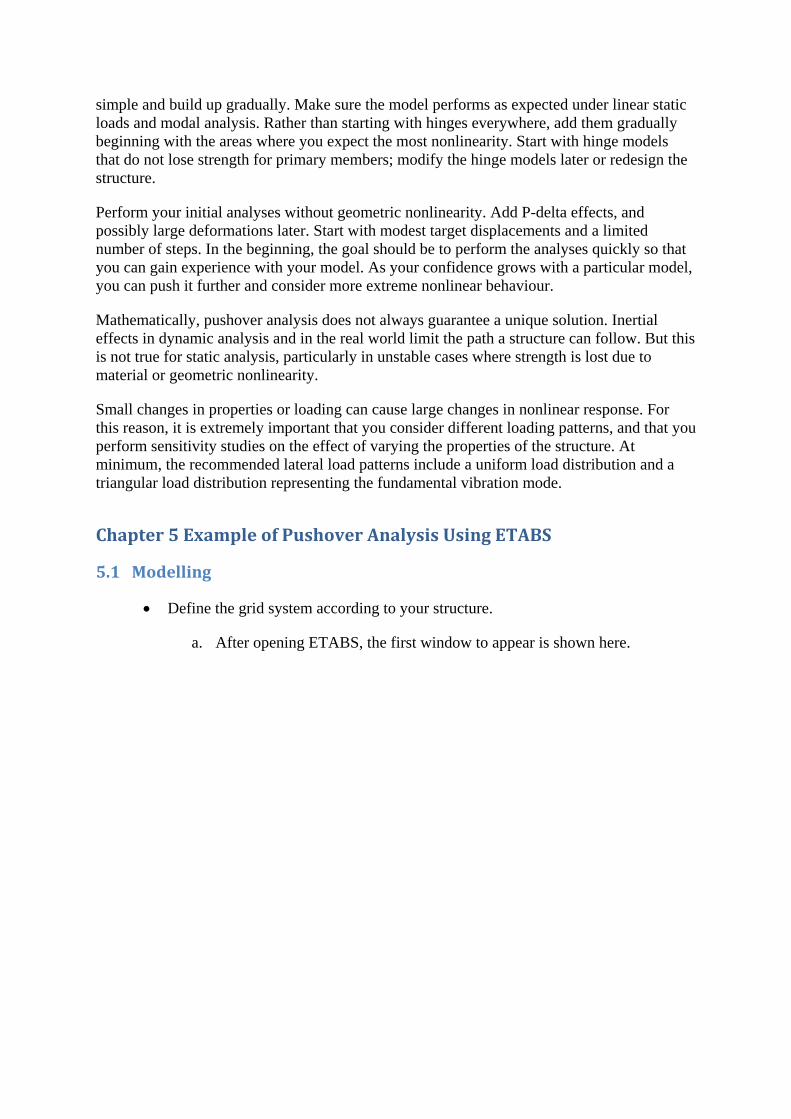
• Define the grid system according to your structure.
a. After opening ETABS, the first window to appear is shown here.

A Practical Guide to Nonlinear Static Analysis
b. Click on FILE followed by DEFAULT.EDB or NO, using the latter
option for a new model.
23
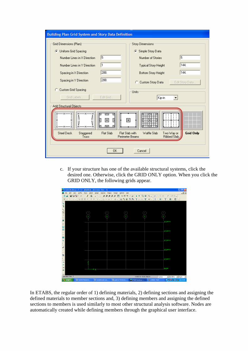
c. If your structure has one of the available structural systems, click the desired one. Otherwise, click the GRID ONLY option. When you click the GRID ONLY, the following grids appear.
In ETABS, the regular order of 1) defining materials, 2) defining sections and assigning the defined materials to member sections and, 3) defining members and assigning the defined sections to members is used similarly to most other structural analysis software. Nodes are automatically created while defining members through the graphical user interface.
A Practical Guide to Nonlinear Static Analysis
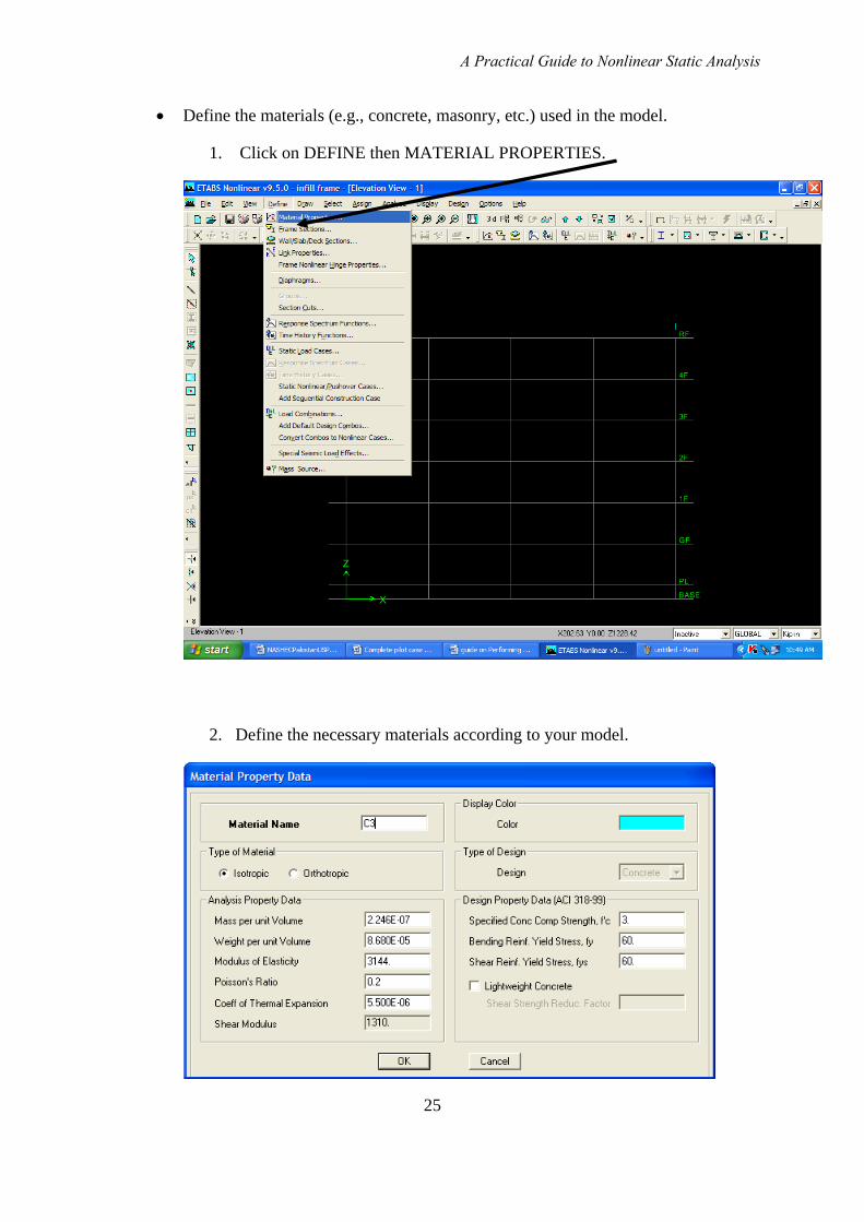
• Define the materials (e.g., concrete, masonry, etc.) used in the model.
1. Click on DEFINE then MATERIAL PROPERTIES.
2. Define the necessary materials according to your model.
25

• Define the frame sections for beams, columns, struts, etc. For masonry struts, use the actual masonry properties, if known, to calculate the equivalent strut capacity. If the actual properties are not known, use the low values in ASCE-41. Parametric studies, where the analyst conducts a series of analyses that vary one property of interest, such as a material strength, while leaving the others fixed, are very useful in bounding the potential response when the masonry properties are not known. Using lower masonry strengths is not necessarily conservative, because stronger infill panels can cause shear failures in the adjacent columns.
a. Click on DEFINE, then FRAME SECTIONS.

A Practical Guide to Nonlinear Static Analysis
b. The following window appears after clicking on FRAME SECTIONS.
27
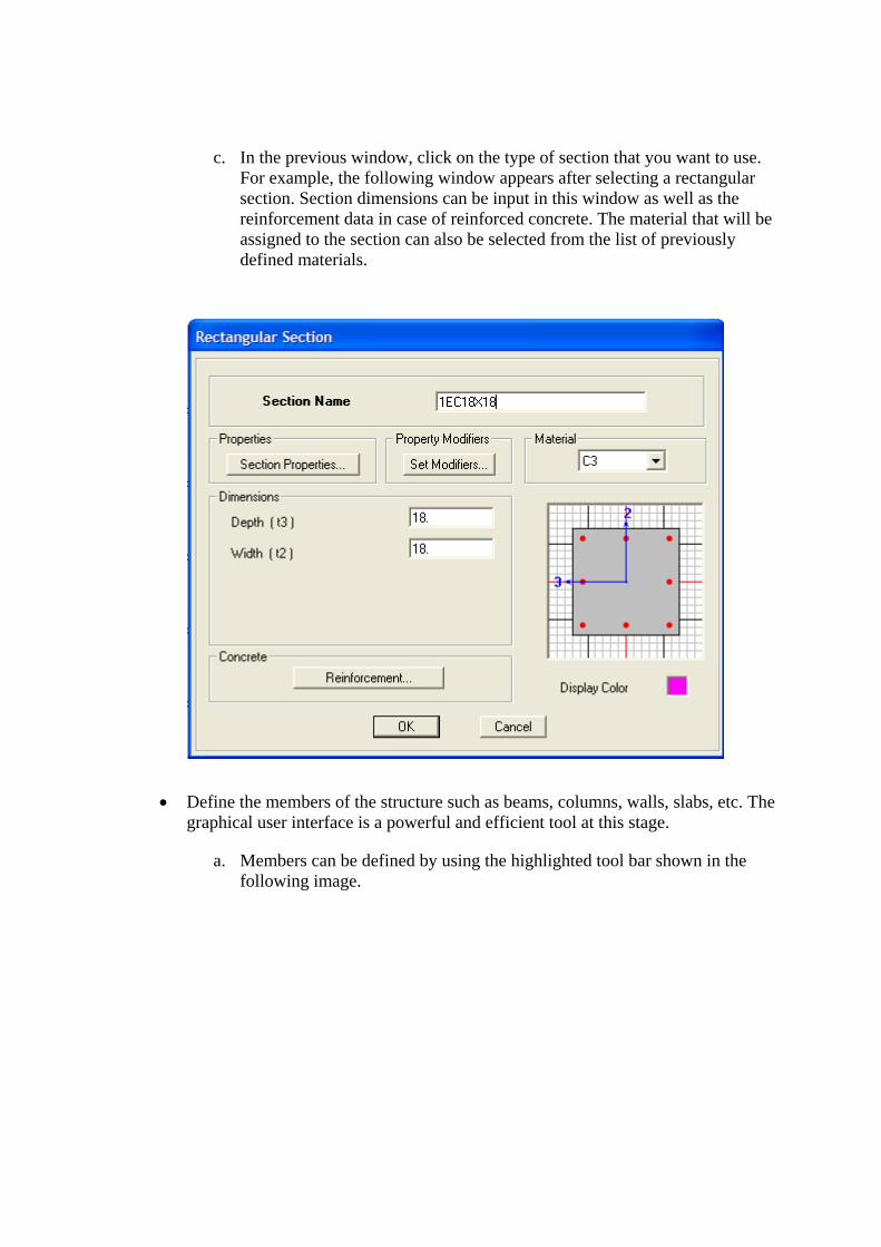
c. In the previous window, click on the type of section that you want to use. For example, the following window appears after selecting a rectangular section. Section dimensions can be input in this window as well as the reinforcement data in case of reinforced concrete. The material that will be assigned to the section can also be selected from the list of previously defined materials.
• Define the members of the structure such as beams, columns, walls, slabs, etc. The graphical user interface is a powerful and efficient tool at this stage.
a. Members can be defined by using the highlighted tool bar shown in the following image.

A Practical Guide to Nonlinear Static Analysis
b. For modelling of beams and columns, you can use line the element tool bar. When you click on this, the following window appears, from which a desired section can be selected.
c. For modelling an RCC wall, an area element tool bar can be used. When
you click on this, the following window appears.
29
5.2 DefiningandAssigningLoadsonStructure
• Apply gravity loads
Dead load and live load factors should be based on the expected gravity loads for the building. For most pushover analyses, use the total dead load and 50% of the live load (1.0 DL + 0.5 LL). You should also check the case of total dead load and zero live load (1.0 DL + 0 LL).
All dead loads in the building (structural components, partitions, architectural finishes and more) should be included in in defining the total dead load. The live load per unit area is accepted as 40, 60 and 100 psf for office buildings, residential buildings and mosques, respectively, per UBC-97, ASCE 7 and many other building design codes.
In this example, the partition load, live load and architectural finishes load are assumed to be 50 psf, 40 psf and 24 psf, respectively. Masonry infill walls should be considered as dead loads, because the infill walls are structural elements.
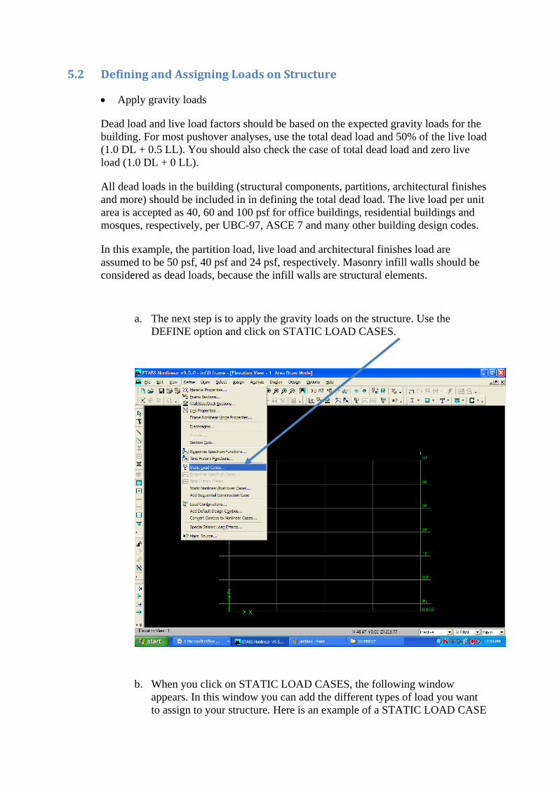
a. The next step is to apply the gravity loads on the structure. Use the DEFINE option and click on STATIC LOAD CASES.
b. When you click on STATIC LOAD CASES, the following window appears. In this window you can add the different types of load you want to assign to your structure. Here is an example of a STATIC LOAD CASE
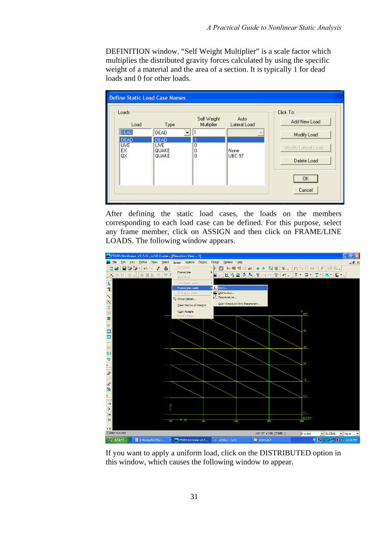
A Practical Guide to Nonlinear Static Analysis
DEFINITION window. “Self Weight Multiplier” is a scale factor which multiplies the distributed gravity forces calculated by using the specific weight of a material and the area of a section. It is typically 1 for dead loads and 0 for other loads.
After defining the static load cases, the loads on the members corresponding to each load case can be defined. For this purpose, select any frame member, click on ASSIGN and then click on FRAME/LINE LOADS. The following window appears.
If you want to apply a uniform load, click on the DISTRIBUTED option in this window, which causes the following window to appear.
31

c. In this window, you can enter the magnitude of loading, its direction and specify the load type.
• Define load combination as per design code.
a. The loads from individual static load cases can be combined using a load combination. Click DEFINE and then LOAD COMBINATION.

A Practical Guide to Nonlinear Static Analysis
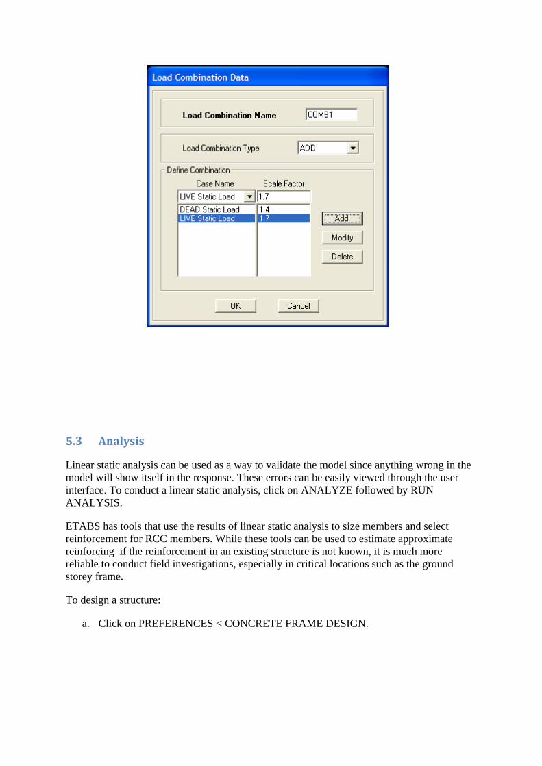
b. When you click on load combination, the following window appears. In this window, click on ADD NEW COMBO
c. When you click on ADD NEW COMBO, the following window appears in
which you can define the load combination as per design code.
33
5.3 Analysis
Linear static analysis can be used as a way to validate the model since anything wrong in the model will show itself in the response. These errors can be easily viewed through the user interface. To conduct a linear static analysis, click on ANALYZE followed by RUN ANALYSIS.
ETABS has tools that use the results of linear static analysis to size members and select reinforcement for RCC members. While these tools can be used to estimate approximate reinforcing if the reinforcement in an existing structure is not known, it is much more reliable to conduct field investigations, especially in critical locations such as the ground storey frame.
To design a structure:
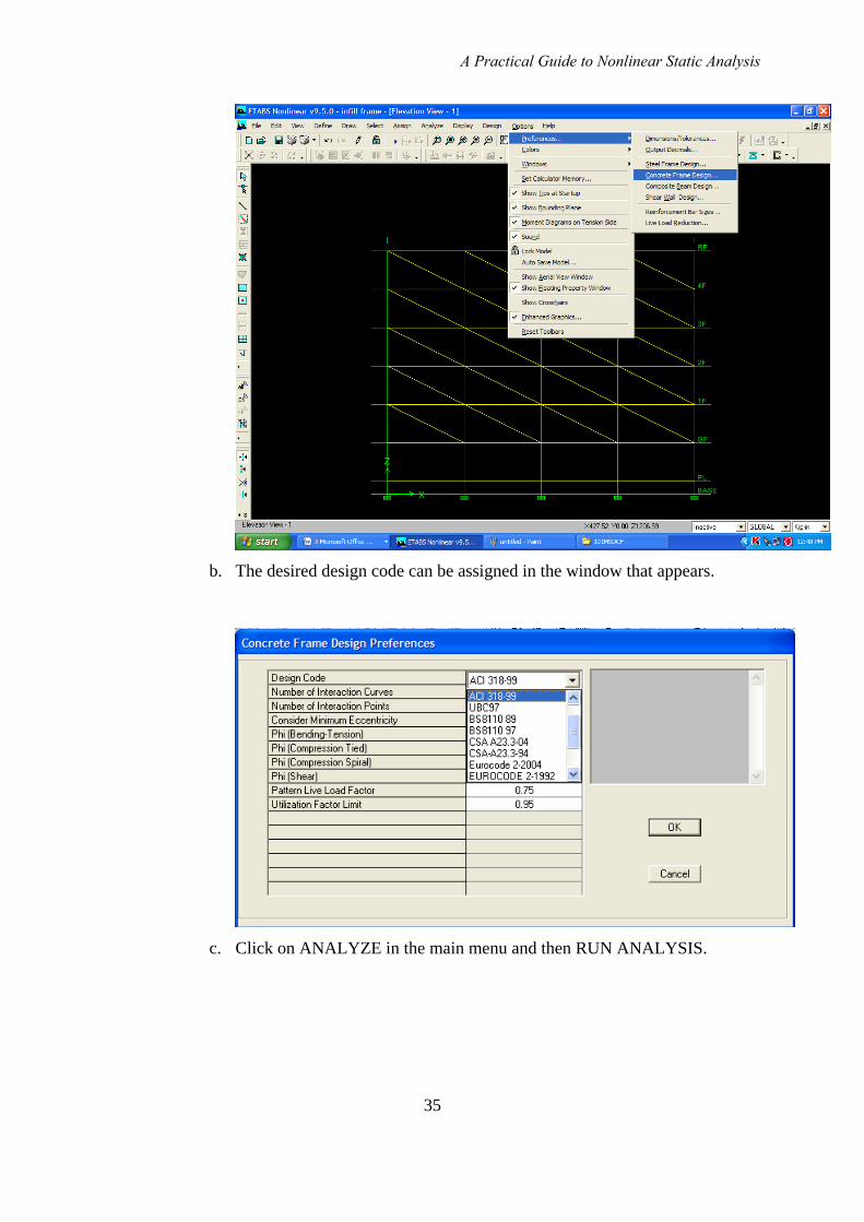
a. Click on PREFERENCES < CONCRETE FRAME DESIGN.
A Practical Guide to Nonlinear Static Analysis
b. The desired design code can be assigned in the window that appears.
c. Click on ANALYZE in the main menu and then RUN ANALYSIS.
35

d. After the analysis, you should design the structure by selecting member sizes and reinforcement. To do that, click on DESIGN < CONCRETE FRAME DESIGN << START DESIGN/CHECK OF STRUCTURE.
e. After obtaining the reinforcement, the moment curvature response of the sections can be determined for use in defining the behaviour of hinges for nonlinear analysis. For an existing structure, this can be done using the available reinforcement. One suitable software program for moment-curvature analysis is RESPONSE 2000.
5.3.2 Non‐LinearStaticAnalysis
• Define the hinge definition in model.
In nonlinear analysis the condition of a structure can be determined on the basis of the hinge status. In ETABS, there are several types of hinges, such as flexural, shear, axial and axial plus flexural. These hinges can be defined and assigned as required. For example, in the following case study, flexural hinges are used for columns and beams and axial hinges are used for struts. Generally, columns should be modelled with coupled axial-flexural (P-M) hinges. For simplicity, shear hinges were not included beams and columns, and the shear failure potential is controlled during post-processing by manually comparing the shear demand from nonlinear static analysis with the shear capacity.

A Practical Guide to Nonlinear Static Analysis
a. To define a hinge, use DEFINE < FRAME NONLINEAR HINGE PROPERTIES
b. When you click on FRAME NONLINEAR HINGE PROPERTIES, the
following window appears. In this window, click on ADD NEW PROPERTY
c. After clicking on ADD NEW PROPERTY, the following window appears. There are options available through which you can define any type of hinge.
37
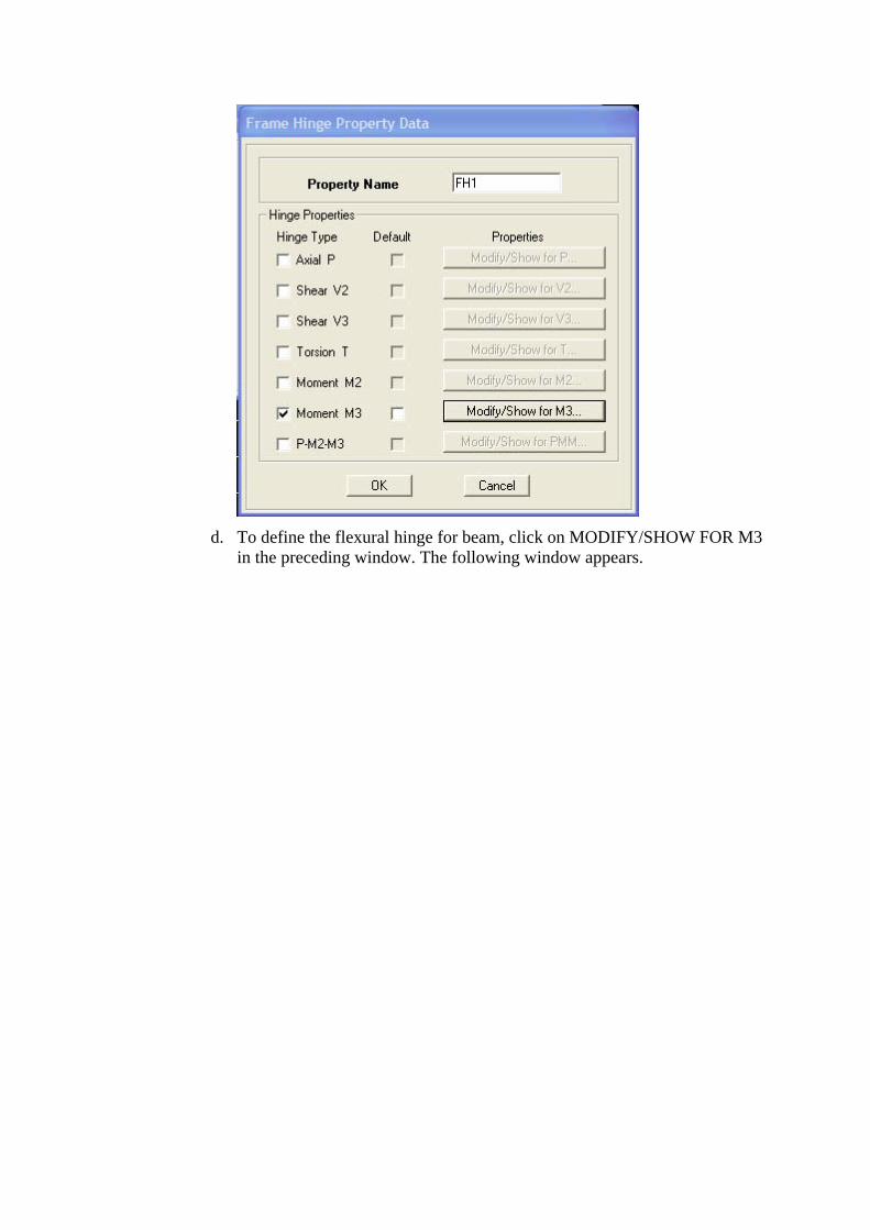
d. To define the flexural hinge for beam, click on MODIFY/SHOW FOR M3
in the preceding window. The following window appears.

A Practical Guide to Nonlinear Static Analysis
Define the hinges using the criteria in ASCE 41. The hinge properties should properly consider the likely as-built conditions, rather that only the design drawings or code provisions. Many buildings in Pakistan and the region will have columns with poor confinement and inadequate ties. Model the hinges conservatively, assuming that the strength and deformation capacity are on the low end of the possible range.
• Assign the hinges in the columns, beams, struts and other structural members.
a. After defining the hinges, the next step is to assign the hinge in the frame elements. Click on ASSIGN < FRAME/LINE < FRAME NONLINEAR HINGES.
39

b. After clicking on FRAME NONLINEAR HINGES, the desired type of
hinge can be assigned to the selected member from the list of defined hinges.
• Define the non-linear static analysis.
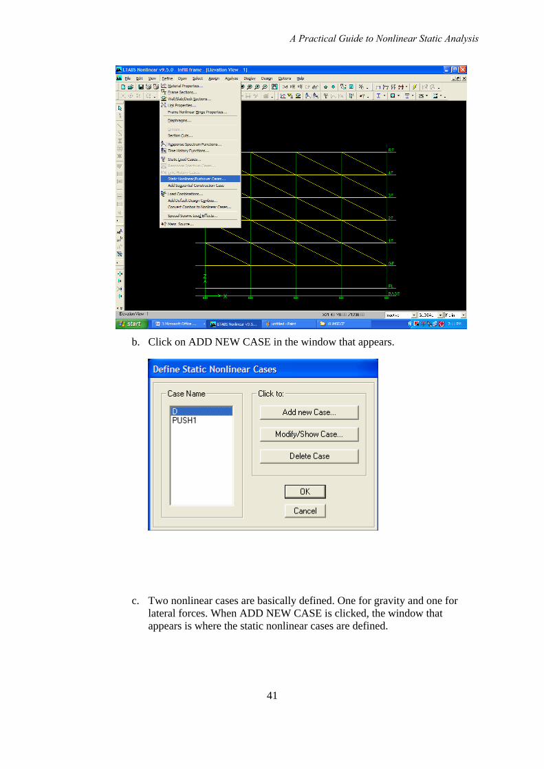
a. After assigning hinges, click on STATIC NONLINEAR PUSHOVER CASES.
A Practical Guide to Nonlinear Static Analysis
b. Click on ADD NEW CASE in the window that appears.
c. Two nonlinear cases are basically defined. One for gravity and one for lateral forces. When ADD NEW CASE is clicked, the window that appears is where the static nonlinear cases are defined.
41

A Practical Guide to Nonlinear Static Analysis
Before proceeding further, there are several terms that need to be defined in the nonlinear static case definition window. The description of the options below is reprinted from the ETABS software documentation.
A. Options
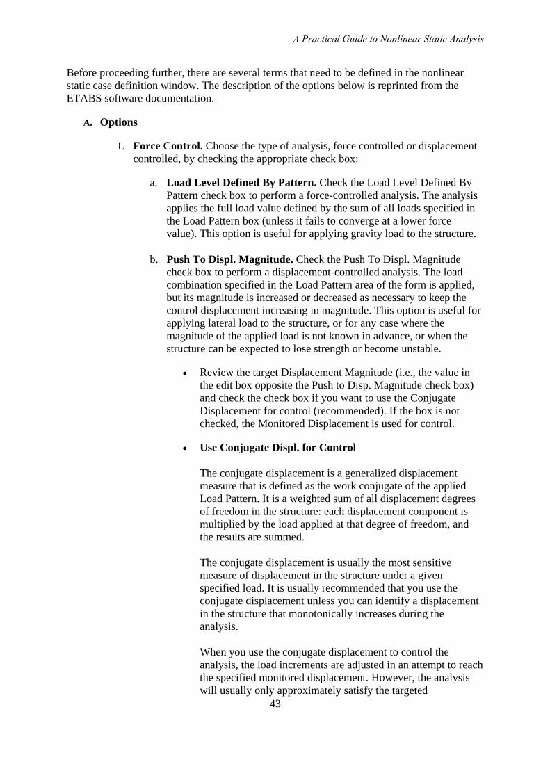
1. Force Control. Choose the type of analysis, force controlled or displacement controlled, by checking the appropriate check box:
a. Load Level Defined By Pattern. Check the Load Level Defined By Pattern check box to perform a force-controlled analysis. The analysis applies the full load value defined by the sum of all loads specified in the Load Pattern box (unless it fails to converge at a lower force value). This option is useful for applying gravity load to the structure.
b. Push To Displ. Magnitude. Check the Push To Displ. Magnitude check box to perform a displacement-controlled analysis. The load combination specified in the Load Pattern area of the form is applied, but its magnitude is increased or decreased as necessary to keep the control displacement increasing in magnitude. This option is useful for applying lateral load to the structure, or for any case where the magnitude of the applied load is not known in advance, or when the structure can be expected to lose strength or become unstable.
• Review the target Displacement Magnitude (i.e., the value in the edit box opposite the Push to Disp. Magnitude check box) and check the check box if you want to use the Conjugate Displacement for control (recommended). If the box is not checked, the Monitored Displacement is used for control.
43
• Use Conjugate Displ. for Control
The conjugate displacement is a generalized displacement measure that is defined as the work conjugate of the applied Load Pattern. It is a weighted sum of all displacement degrees of freedom in the structure: each displacement component is multiplied by the load applied at that degree of freedom, and the results are summed.
The conjugate displacement is usually the most sensitive measure of displacement in the structure under a given specified load. It is usually recommended that you use the conjugate displacement unless you can identify a displacement in the structure that monotonically increases during the analysis.
When you use the conjugate displacement to control the analysis, the load increments are adjusted in an attempt to reach the specified monitored displacement. However, the analysis will usually only approximately satisfy the targeted

displacement, particularly if the monitored displacement is in a different direction than the conjugate displacement.
• Monitor
Define the Monitored Displacement by selecting the displacement degree of freedom, and by entering the label and selecting the story level of the point to be monitored. The Monitored Displacement is used to plot the pushover curve and also for displacement control when the Push To Displ. Magnitude option is used.
The Monitored Displacement is a single displacement component at a single point that is monitored during a static nonlinear analysis. When plotting the pushover curve, the program always uses the monitored displacement for the horizontal axis. The monitored displacement is also used to determine when to terminate a displacement-controlled analysis.
The monitored degree of freedom and the monitored point location are all given default values by ETABS; you can easily replace those default values. The default value for the monitored point is a point located at the top of the structure; use this point for infill frame buildings. The default monitored degree of freedom is UX; other available directions are UY, UZ, RX, RY, and RZ.
For the most meaningful pushover curve, it is important that you choose a monitored displacement that is sensitive to the applied load pattern. For example, you should not typically monitor degree of freedom UX when the load is applied in direction UY. Likewise you should not monitor joints that are close to the restraints.
The same considerations apply when choosing a monitored displacement for the purposes of displacement control. Choose a displacement that is sensitive to the applied load and, if possible, one that increases monotonically during the analysis.
You may use the monitored displacement or the conjugate displacement for displacement control, but it is the magnitude of the monitored displacement that is used to determine when to terminate a displacement-controlled analysis.
When you use the conjugate displacement to control the analysis, the load increments are adjusted in an attempt to reach the specified monitored displacement. However, the analysis will usually only approximately satisfy the targeted displacement, particularly if the monitored displacement is in a
A Practical Guide to Nonlinear Static Analysis
different direction than the conjugate displacement. For the typical first mode or triangular load pattern, it is suitable to use the roof displacement in the lateral load direction as the monitored displacement
The analysis is terminated when the Monitored Displacement reaches the specified Displacement Magnitude (unless it fails to converge at a lower displacement value).
The target Displacement Magnitude for the Monitored Displacement is given a default value by ETABS of 0.04 times the Z coordinate at the top of the structure. Note that if the base of the structure has a Z coordinate greater than zero, the default displacement may be quite large. You may change this value as necessary. Only the absolute value of the Displacement Magnitude is used: the direction of loading is determined by the specified load pattern.
2. Start from Previous Case. To start the current case from the end condition of a previously specified static nonlinear case, select the name of the previous case from the Start From Previous Case drop down list. Typically this option is used for a lateral static nonlinear case to specify that it should start from the end of a gravity static nonlinear case.
3. Save Positive Increments Only. If you want only positive displacement increments of the pushover curve to be saved, check the Save Positive Increments Only check box. For the typical first mode or triangular load pattern and roof displacement used as the monitored displacement, this option is sufficient.
4. Review the following analysis control parameters, changing them if necessary. In general, start with smaller limits on the maximums, increasing them as you gain experience with your model.
• Minimum Saved Steps
The Minimum Saved Steps restricts the maximum step size used to apply the load in a static nonlinear case. ETABS automatically creates steps corresponding to events on the hinge stress-strain curves or to significant nonlinear geometric effects. The results of these steps are saved only if they correspond to a significant change in the slope of the pushover curve.
You can use the Minimum Saved Steps to force the program to save additional steps. A value between 5 and 20 is adequate for most cases, although if you expect a lot of hinge events, a value of 1 is often the
45

best. If the Member Unloading Method is set to Restart Using Secant Stiffness, a value of 1 is also recommended.
• Maximum Null Steps
The Maximum Null Steps is used, if necessary, to declare failure (i.e., non-convergence) in a run before it reaches the specified force or displacement goal. The program may be unable to converge on a step when catastrophic failure occurs in the structure, or when the load cannot be increased in a load-controlled analysis. There may also be instances where it is unable to converge in a step because of numerical sensitivity in the solution.
There are four types of null steps.
1. When an event in one hinge changes the stiffness of the structure such that another hinge has an immediate event. This shows up as zero-length step.
2. When the Member Unloading Method is set to Unload Entire Structure and the unloading of a hinge causes a reversal in the direction of load applied to the structure. This shows up as zero-length step.
3. When the Member Unloading Method is set to Apply Local Redistribution and the unloading of a hinge causes the application and removal of an internal local redistribution load. This shows up as multiple zero-length steps.
4. When a step fails to converge within the Maximum Iteration/Step and the step size is halved. This is not a zero-length step.
Null steps are to be expected in any analysis; they are not necessarily bad. However, an excessive number of them may indicate failure of the analysis.
Typically the Maximum Null Steps should be set to about 25% of the Maximum Total Steps (e.g., the default is 50 Maximum Null Steps for 200 Maximum Total Steps), but you may need at least twice as many when the Member Unloading Method is set to Apply Local Redistribution. Significant Large Displacement effects may also require more null steps.
• Maximum Total Steps
The Maximum Total Steps limits the total time the analysis will be allowed to run.

A Practical Guide to Nonlinear Static Analysis
ETABS attempts to apply as much of the specified load pattern as possible but may be restricted by the occurrence of an event, failure to converge within the Maximum Iterations/Step, or a limit on the maximum step size from the Minimum Number of Saved Steps. As a result, a typical static nonlinear analysis may consist of a large number of steps. Additional steps may be required by some Member Unloading Methods to redistribute load.
An event occurs whenever a hinge reaches a new point on its stress-strain curve or elastically unloads. Thus the number of steps required to reach a specified target load or displacement will increase with the number of hinges in the model.
Each step takes about the same amount of computer time. As you gain experience with a particular model, you will be able to set the Maximum Total Steps to limit the time the static nonlinear analysis is allowed to run. You should start small and gradually build up to larger numbers of steps.
If your analysis does not reach its target within the Maximum Total Steps, you can run it again with a larger number of steps, but first examine the results to see whether the structure is still stable enough to be worth pushing it any farther.
Only steps resulting in significant changes in the shape of the pushover curve are saved for output.
5. Review the following analysis control parameters, changing them if necessary. In most cases, the default values are adequate.
• Maximum Iterations/Step and Iteration Tolerance
Static equilibrium is checked at the end of each step in a static nonlinear analysis. The unbalanced load is calculated as the difference between the externally applied loads and the internal forces in the elements. If the ratio of the unbalanced-load magnitude to the applied-load magnitude exceeds the Iteration Tolerance, the unbalanced load is applied to the structure in a second iteration for that step. These iterations continue until the unbalanced load satisfies the Iteration Tolerance or the Maximum Iterations/Step is reached. In the latter case, the step size is halved and the load is applied again from the beginning of the step.
If necessary, the step size is continuously halved until equilibrium is finally achieved. Each halving of the step size counts as a null step. For the next step after convergence, the program repeatedly doubles the step size until it finds the largest size that will converge or until an event occurs.
47

Iteration is primarily activated by nonlinear link properties and by geometric nonlinearity, especially for large-displacement analysis. Iteration is not usually required for material nonlinearity in the frame hinges because of the event-to-event strategy used.
• Event Tolerance
The Event Tolerance is a ratio used to determine the lumping together of events. When ETABS determines that one hinge has experienced an event, it checks for other hinges that are close (within the Event Tolerance) to experiencing an event. For all hinges within the Event Tolerance, the program will modify their states to cause these nearby events to occur.
Larger event tolerances can shorten analysis time by reducing the number of steps caused by events, but can increase equilibrium errors within the elements due to the modification of the hinge states. Smaller event tolerances give more accurate results at the expense of more computational time. The default value of 0.01 works well for most cases.
Consider the figure, which shows the location of two hinges on their force-displacement plots. Hinge 1 has reached an event location. For hinge 2, if the Event Tolerance is met it too will be treated as part of the event. In the figure, if the Force Tolerance divided by the Yield Force is less than the Event Tolerance, and the Displacement Tolerance divided by the horizontal distance from B to C is less than the Event Tolerance, then hinge 2 will be treated as part of the event. When determining the Force Tolerance Ratio, the denominator is always the yield force. When determining the Displacement Tolerance Ratio, the denominator is the horizontal length of the portion of the force-displacement curve that the hinge is currently on. In the figure, hinge 2 is on the B-C portion of the curve, thus we used the B-C horizontal length in the denominator of the Displacement Tolerance Ratio.
B. Member Unloading Method
1. Select the method to be used to handle hinges that drop load. This may affect the number of steps you allow for the analysis.
When a hinge unloads, the program must find a way to remove the load that the hinge was carrying and possibly redistribute it to the rest of the structure. Hinge unloading occurs whenever the stress-strain (force-deformation or moment-rotation) curve shows a drop in capacity, such as is often assumed from point C to point D, or from point E to point F (complete rupture).
Such unloading along a negative slope is unstable in a static analysis, and a unique solution is not always mathematically guaranteed. In dynamic analysis (and the real world) inertia provides stability and a unique solution.
A Practical Guide to Nonlinear Static Analysis
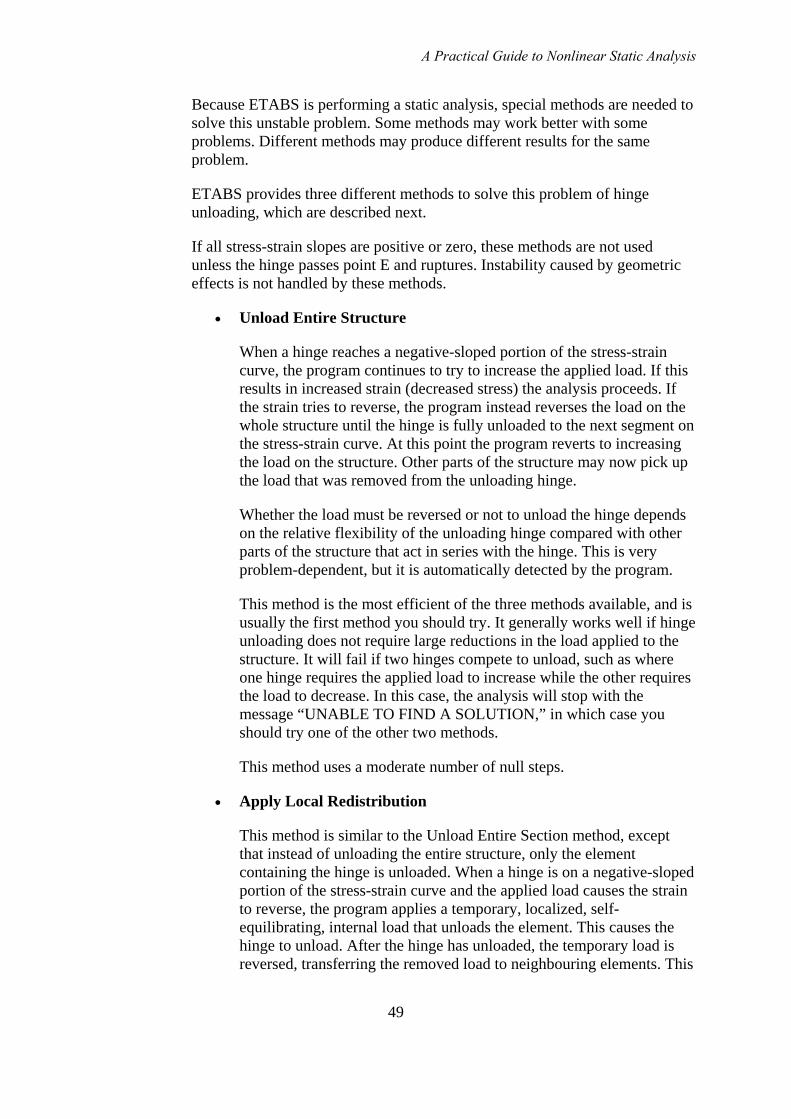
Because ETABS is performing a static analysis, special methods are needed to solve this unstable problem. Some methods may work better with some problems. Different methods may produce different results for the same problem.
ETABS provides three different methods to solve this problem of hinge unloading, which are described next.
If all stress-strain slopes are positive or zero, these methods are not used unless the hinge passes point E and ruptures. Instability caused by geometric effects is not handled by these methods.
• Unload Entire Structure
When a hinge reaches a negative-sloped portion of the stress-strain curve, the program continues to try to increase the applied load. If this results in increased strain (decreased stress) the analysis proceeds. If the strain tries to reverse, the program instead reverses the load on the whole structure until the hinge is fully unloaded to the next segment on the stress-strain curve. At this point the program reverts to increasing the load on the structure. Other parts of the structure may now pick up the load that was removed from the unloading hinge.
Whether the load must be reversed or not to unload the hinge depends on the relative flexibility of the unloading hinge compared with other parts of the structure that act in series with the hinge. This is very problem-dependent, but it is automatically detected by the program.
This method is the most efficient of the three methods available, and is usually the first method you should try. It generally works well if hinge unloading does not require large reductions in the load applied to the structure. It will fail if two hinges compete to unload, such as where one hinge requires the applied load to increase while the other requires the load to decrease. In this case, the analysis will stop with the message “UNABLE TO FIND A SOLUTION,” in which case you should try one of the other two methods.
This method uses a moderate number of null steps.
• Apply Local Redistribution
This method is similar to the Unload Entire Section method, except that instead of unloading the entire structure, only the element containing the hinge is unloaded. When a hinge is on a negative-sloped portion of the stress-strain curve and the applied load causes the strain to reverse, the program applies a temporary, localized, self-equilibrating, internal load that unloads the element. This causes the hinge to unload. After the hinge has unloaded, the temporary load is reversed, transferring the removed load to neighbouring elements. This
49
process is intended to imitate how local inertia forces might stabilize a rapidly unloading element.
This method is often the most effective of the three methods available, but usually requires more steps than the first method, including a lot of very small steps and a lot of null steps. The limit on null steps should usually be set between 40% and 70% of the total steps allowed.
This method will fail if two hinges in the same element compete to unload, such as where one hinge requires the temporary load to increase while the other requires the load to decrease. In this case, the analysis will stop with the message “UNABLE TO FIND A SOLUTION,” after which you should divide the element so the hinges are separated and try again. Check the .LOG file to see which elements are having problems. Caution: the element length may affect default hinge properties that are automatically calculated by the program, so fixed hinge properties should be assigned to any elements that are to be divided.
• Restart Using Secant Stiffness
This method is quite different from the other two. Whenever any hinge reaches a negative-sloped portion of the stress-strain curve, all hinges that have become nonlinear are reformed using secant stiffness properties, and the analysis is restarted.
The secant stiffness for each hinge is determined as the secant from point O to point X on the stress strain curve, where: Point O is the stress-stain point at the beginning of the static nonlinear case (which usually includes the stress due to gravity load); and Point X is the current point on the stress-strain curve if the slope is zero or positive, or else it is the point at the bottom end of a negatively-sloping segment of the stress-strain curve.
When the load is re-applied from the beginning of the analysis, each hinge moves along the secant until it reaches point X, after which the hinge resumes using the given stress-strain curve.
This method is similar to the approach suggested by the FEMA 273 guidelines, and makes sense when performing pushover analysis where the static nonlinear analysis represents cyclic loading of increasing amplitude rather than a monotonic static push.
This method is the least efficient of the three, with the number of steps required increasing as the square of the target displacement. It is also the most robust (least likely to fail) provided that the gravity load is not too large. This method may fail when the stress in a hinge under gravity load is large enough that the secant from O to X is negative. On the other hand, this method may also give solutions where the other two fail due to hinges with small (nearly horizontal) negative slopes.

A Practical Guide to Nonlinear Static Analysis
C. Geometric Nonlinearity Effects
1. Select the Geometric Nonlinearity Effects to be included. Geometric nonlinearity effects are considered on all elements in the structure. The following options are available:
The large displacement option should be used for cable structures undergoing significant deformation; and for buckling analysis, particularly for snap-through buckling and post-buckling behaviour. Cables (modelled by frame elements) and other elements that undergo significant relative rotations within the element should be divided into smaller elements to satisfy the requirement that the strains and rotations within an element are small.
For most other structures, the P-delta option is adequate, particularly when material nonlinearity dominates. If reasonable, it is recommended that the analysis be performed first without P-delta (i.e., use None), adding geometric nonlinearity effects later.
• None All equilibrium equations are considered in the undeformed configuration of the structure.
• P-Delta The equilibrium equations take into partial account the deformed configuration of the structure. Tensile forces tend to resist the rotation of elements and stiffen the structure, and compressive forces tend to enhance the rotation of elements and destabilize the structure. This may require a moderate amount of iteration.
• P-Delta and Large Displacements All equilibrium equations are written in the deformed configuration of the structure. This may require a large amount of iteration.
D. Load Pattern
One of the most difficult issues for pushover analysis is choosing the pushover load distribution. During an actual earthquake, the effective loads on a structure change continuously in magnitude, distribution and direction. The distribution of story shears over the height of a building can thus change substantially with time, especially for taller buildings where higher modes of vibration can have significant effects. In a static pushover analysis, the distribution and direction of the loads are fixed, and only the magnitude varies. Hence, the distribution of story shears stays constant. To account for different story shear distributions, it is necessary to consider a number of different pushover load distributions.
One option in FEMA 356 is to use uniform and triangular distributions over the building height. Note that a uniform distribution usually corresponds to a uniform acceleration over the building height, so that the load at any floor level is proportional to the mass at the floor. Similarly, a triangular distribution usually corresponds to a linearly increasing acceleration over the building height.
51

In ETABS the distribution of load applied on the structure for a given static nonlinear case is defined as a scaled combination of one or more of the following:
• Any static load case.
• A uniform acceleration acting in any of the three global directions. The force at each joint is proportional to the mass tributary to that joint and acts in the specified direction.
• A modal load for any eigen or Ritz mode. The force at each joint is proportional to the product of the modal displacement, the modal circular frequency squared (�2), and the mass tributary to that joint, and it acts in the direction of the modal displacement.
The load combination for each static nonlinear case is incremental, meaning it acts in addition to the load already on the structure if starting from a previous static nonlinear case.
Add, modify or delete a Load Pattern for the static nonlinear case using the following buttons.
• Add button. To add a Load to the Load Pattern definition, select the load from the Load drop down box, type in the appropriate scale factor in Scale Factor edit box, and click the Add button. If the selected load is a mode (only available if mode shapes have been requested for the analysis), input the mode shape in the resulting form and click the OK button.
• Modify button. To modify the scale factor for a load specified as part of the load pattern, highlight the load in the Load/Scale Factor list box, edit the scale factor in the Scale Factor edit box, and click the Modify button.Delete button. To delete a load specified as part of the load pattern, highlight the load in the Load/Scale Factor list box and click the Delete button.
Click the OK button to accept all of the changes made in the Static Nonlinear Case Data form. Clicking the Cancel button means that none of the changes will be accepted. Note that you must also click the OK button in the Define Static Nonlinear Cases form to accept the changes.
Run the non-linear static analysis. Click the ANALYZE option, RUN STATIC NONLINEAR ANALYSIS. During the analysis, sometimes there is a warning in nonlinear analysis. You should stop the analysis and increase the number of null steps and total steps in nonlinear static data form and again run the analysis.
A Practical Guide to Nonlinear Static Analysis
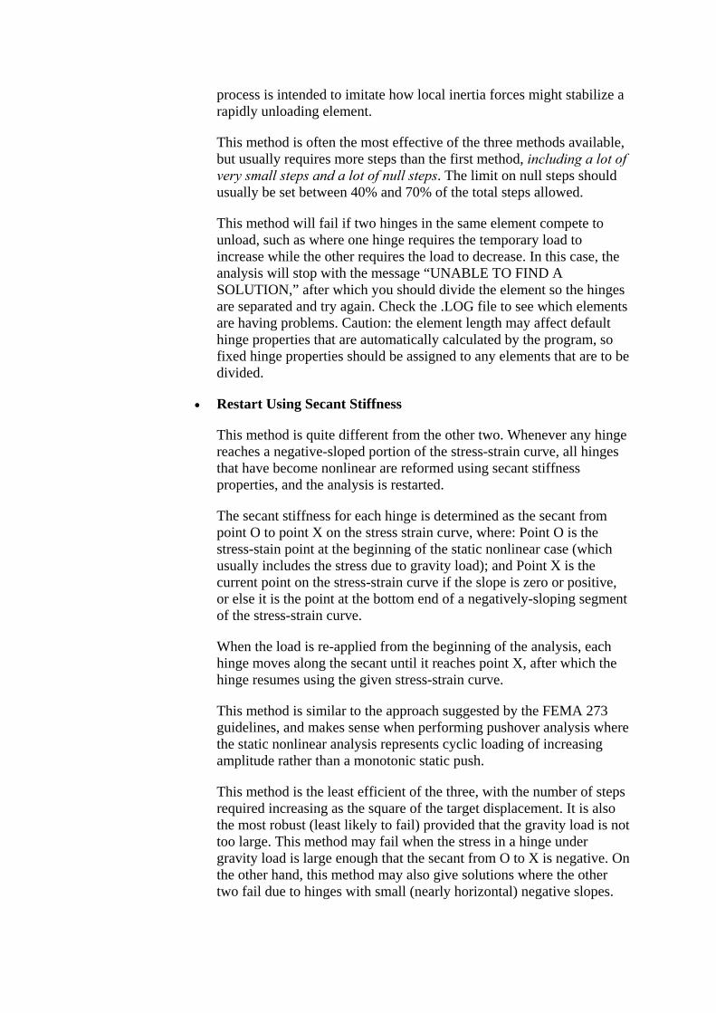
5.4 Results
• Check the pushover curve and capacity curve.
a. After the analysis, check the results by clicking on DISPLAY < SHOW STATIC PUSHOVER CURVE.
53

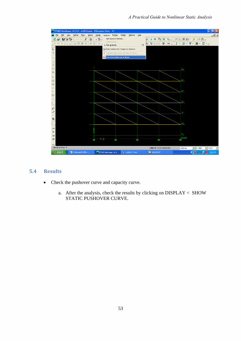
b. When we click on SHOW STATIC PUSHOVER CURVE, the following window appears.
A Practical Guide to Nonlinear Static Analysis
• Check the deformed shape of the structure at the performance point.
The performance point is the point at which the demand spectra and capacity spectra intersect each other. At that point, we have to check if the structure can meet the demand or not.
a. Next step is to check the number of steps at which the demand and capacity curves intersect. At that step display, the deformed shape by clicking on DISPLAY < SHOW DEFORMED SHAPE.
55
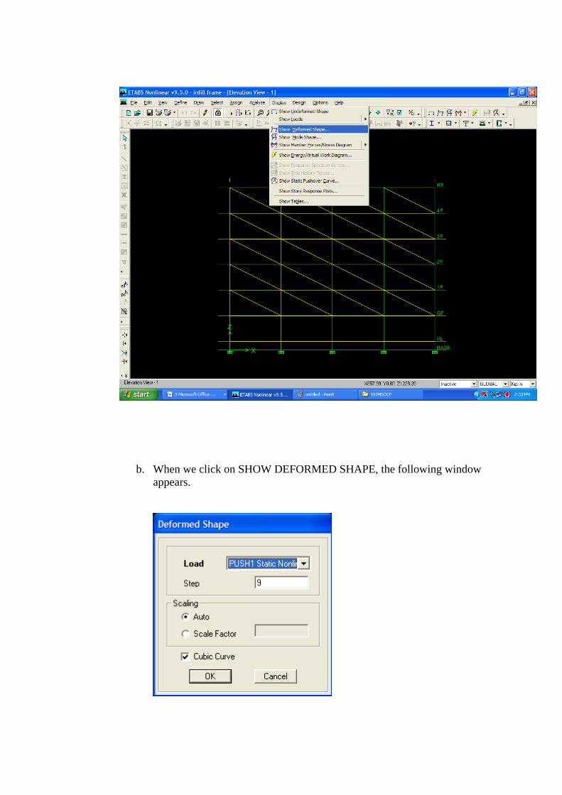
b. When we click on SHOW DEFORMED SHAPE, the following window appears.

A Practical Guide to Nonlinear Static Analysis
c. In the previous window, set the case and step number and the following window appears.
• Check the status of the internal hinges
Check the status of hinges to see if the structure can meet the demand or not. Based on the hinge states and the failure mechanisms, the need for retrofit and the type of retrofit can be determined.
The colour of hinges defines the status of hinges.
This building needs a retrofit to prevent the soft story from forming. Once you have created a model, it is straightforward to modify it by adding new elements in different places to test out potential retrofit solutions.
57

Sources of Additional Information
As the example in the previous chapter shows, nonlinear analysis is a powerful tool to examine the expected behaviour of a building during a strong earthquake. The building shown in the example needed a seismic retrofit, and a retrofit solution was selected by testing a number of different retrofit options in ETABS. FEMA 547, Techniques for the Seismic Rehabilitation of Buildings, which is available free of charge from www.fema.gov, provides detailed information on potential retrofit solutions and how to select them. Also, the reports on buildings analyzed as case studies during the Pakistan-US cooperative project provide detailed examples of retrofit solutions for typical Pakistani buildings. These reports can be downloaded from the GeoHazards International website at www.geohaz.org. Additional detailed information about nonlinear analysis can be found in the NEHRP Seismic Design Technical Brief No. 4, Nonlinear Structural Analysis for Seismic Design: A Guide for Practicing Engineers, available free of charge from www.nehrp.gov.

A Practical Guide to Nonlinear Static Analysis
References
1. ETABS, User Interface Reference Manual. 2002, Computers & Structures (CSi): California.
2. Federal Emergency Management Agency, FEMA-356: Prestandard and Commentary for the Seismic Rehabilitation of Buildings. 2000: Washington DC.
3. American Society of Civil Engineers, ASCE-41: Seismic Rehabilitation of Existing Buildings. 2006: Virginia.
4. Applied Technology Council, ATC-40: Seismic Evaluation and Retrofit of Concrete Buildings. 1996: California.
5. Humar, J.M., D. Lau, and J.-R. Pierre, Performance of buildings during the 2001 Bhuj earthquake. Canadian Journal of Civil Engineering, 2001. 28(6): p. 979-991.
6. Korkmaz, K.A., F. Demir, and M. Sivri, Earthquake Assessment of R / C Structures with Masonry Infill Walls. International Journal of Science and Technology, 2007. 2: p. 155-164.
7. Mondal, G. and S.K. Jain, Lateral Stiffness of Masonry Infilled Reinforced Concrete (RC) Frames with Central Opening. Earthquake Spectra, 2008. 24(3): p. 701.
8. Saatcioglu, M., et al., The August 17, 1999, Kocaeli (Turkey) earthquake — damage to structures. Canadian Journal of Civil Engineering, 2001. 28(4): p. 715-737.
9. Taher, S.E.-D.F. and H.M.E.-D. Afefy, ROLE OF MASONRY INFILL IN SEISMIC RESISTANCE OF RC STRUCTURES. The Arabian Journal for Science and Engineering, 2008. 33: p. 291-306.
12. Murty, C.V.R., et al., AT RISK : The Seismic Performance of Reinforced Concrete Frame Buildings with Masonry Infill Walls. 2006, Earthquake Engineering Research Institute and the International Association for Earthquake Engineering: Oakland. p. 83.
13. Kodur, V.K.R., M.A. Erki, and J.H.P. Quenneville, Seismic design and analysis of masonry-infilled frames. Canadian Journal of Civil Engineering, 1995. 22(3): p. 576-587.
59