Embed Size (px)
Citation preview

THE SKILL OF BICYCLE RIDING
Anthony John Redfern Doyle
Department of psychology, University of Sheffield
Submitted in part fulfilment of the requirements of the degree of PhD.
March 1987

SUMMARY
The Skill of Bicycle Riding
A.J.R. Doyle
The principal theories of human motor skill are compared. Disagreements between them centre around the exact details of the feedback loops used for control. In order to throw some light on this problem a commonplace skill was analysed using computer techniques to both record and model the movement. Bicycle riding was chosen as an example because it places strict constraints on the freedom of the rider's actions and consequently allows a fairly simple model to be used. Given these constraints a faithful record of the delicate balancing movements of the handlebar must also be a record of the rider's actions in controlling the machine.
An instrument pack, fitted with gyroscopic sensors and a handlebar potentiometer, recorded the roll, yaw and steering angle changes during free riding in digital form on a microcomputer disc. A discrete step computer model of the rider and machine was used to compare the output characteristic of various control systems with that of the experimental subjects. Since the normal bicycle design gives a measure of automatic stability it is not possible to tell how much of the handlebar movement is due to the rider and how much to the machine. Consequently a bicycle was constructed in which the gyroscopic and castor stability were removed. In order to reduce the number of sensory contributions the subjects were blindfolded.
The recordings showed that the basic method of control was a combination of a continuous delayed repeat of the roll angle rate in the handle-bar channel, with short intermittent ballistic acceleration inputs to control angle of lean and consequently direction.
A review of the relevant literature leads to the conclusion that the proposed control system is consistent with current physiological knowledge. Finally the bicycle control system discovered in the experiments is related to the theories of motor skills discussed in the second chapter.
Acknowledgements
This thesis was supported by a studentship grant from
the Science and Engineering Research Council. I gratefully
acknowledge the direction and support of my supervisor
Professor Kevin Connolly. I would also like to thank Bob
Chapman and Mick Cruse of the psychology technical
department for turning my vague notions into working
hardware, and especial thanks is due to Michael Port who
not only constructed the recording module and kept it
running, but also showed great patience in acting as one
of the test subjects.
Professor Linkens of the Control Engineering department
provided generous support, as did Dr. Neal of the
Mechanical Engineering department. I would also like to
thank my son James, my daughter Harriet and my
granddaughter Hannah for acting as experimental subjects.
I would very much like to thank Chris Brown and Max
Westby for their quite exceptional patience and generous
help under a bombardment of questions while I was
acquiring the computing skills on which this study
depended. I would like to extend similar thanks to Adrian
Simpson for being so tolerant and helpful with statistical
advice to, John Elliott for all his help and encouragement
in the early days of the project and to Judy Doyle and
Vicki Bruce for checking the final script.

CONTENTS
Chapters
1 Introduction 1
2 Motor Behaviour Research 4
3 Bicycle Riding as an Example of Human Skill 25
4 The Computer Model 55
5 The Calibrated Bicycle 85
6 Simulation of the Destabilized Bicycle Control 119
7 Control of the Autostable Bicycle 168
8 The Biological Correlates of the Control System 198
9 The Organization of Control
References
Appendices
234
254
l(a) The Simulator Programs 260
l(b) Scale Drawing of the Destabilized Bicycle. 272
2(a) Roll and bar angles. 274
2(b) Roll and bar rates.
2(c) Histograms of lag, half-wave & area.
3(a) Effect of Gain on Stability.
3(b) Regression residuals plots.
3(c) Relation between residuals & roll angle.
281
294
300
305
312

Bicycle Riding Chapter 1
1. INTRODUCTION
Much of the research into motor behaviour starts from
some theoretical position and explores the adequacy of
this experimentally. A task is chosen either because it
offers some specific advantage in the laboratory in terms
of ease of recording the variables or because it focuses
on some detail of particular interest to the theoretical
argument. Most naturally arising skills are too complex
and loosely defined to be examined in toto. The hope is
that rules of operation will appear in the laboratory
experiments which can then be used as primitive building
blocks from which complete skills can be synthesized.
This study starts from the opposite position. It takes
a naturally arising skill and attempts to analyse it so
that a determinate system model will accurately predict
the behaviour, over time, of a selected set of variables
measured on the real machine. Bicycle riding was chosen
because its inherent unstability allows only a few
alternative strategies of operation.
The word system appears frequently in the following
text in a number of different contexts. In its normal use,
such as in nervous system it is rather loosely defined to
mean a large number of parts connected together in a
determinate way to act as a complex whole. When it applies
to the bicycle control problem I will attempt to follow
Ross Ashby's tighter definition (1952, 2/4, page 15) by
using the word to refer to that particular set of
variables chosen by the experimenter to represent some
event in the real world. Thus the changes in lean angle
and steering angle over time recorded from a bicycle
constitute a system representing that particular part of
its behaviour, although, as will be shown, this system is
too limited to be state-determined and other variables
1

Bicycle Riding Chapter 1
must be added to form a system capable of accurate
predictions.
The first chapter is a review of the various general
theoretical approaches to skilled motor movements to which
the particular details of this study will be related in
the final chapter.
The second chapter deals with the specific control
problems that arise from the nature of the rider/bicycle
combination regarded as a mechanical system. It reviews
some of the engineering research that has been done into
the bicycle and touches on the psychological research into
feedback control loops in humans.
Chapter three describes in detail the computer
simulation of the bicycle which is used to test various
control systems for their effect on the general
characteristics of the bicycle/rider unit in later
chapters.
The next two chapters use the records from a specially
constructed bicycle to show in detail what a control
system must do to achieve slow-speed, straight-line
riding. In order to guarantee that all the control
movements of the riders were recorded and that these were
the only movements being used for control, the automatic
stability provided by the front forks of the normal
bicycle was removed to create a 'zero-stable' bicycle. It
was found that in the absence of built-in stability the
riders themselves provided sufficient for control. The
analysis shows that the principle control of roll velocity
for lateral stability was continuous but argues that there
is strong evidence that an intermittent movement
superimposed upon this underlying action was being used to
control the angle of lean. When the proposed control
solution was implemented on a simulation of the
destabilized bicycle it produced an output characteristic
almost identical with that obtained from the real riders.
2

Bicycle Riding
Chapter six
by the runs
Chapter 1
considers how the control system suggested
with the destabilized bicycle relates to
riding a normal bicycle. A comparison with an exactly
similar set of runs on an unmodified bicycle indicated
that there was little difference between the two in the
slow straight-ahead case, the automatic control being
relatively ineffective at very low speed. The general
interest in bicycle control must obviously focus on
manoeuvring at normal riding speeds and the original hope
had been to examine the effects of increased speed and
manoeuvre on both types of machine. Unfortunately, lack
of time prevented any further recording, and the only
successful record of a manoeuvring run available was one
made during the early pilot tests. The information from
this run together with some general observations of
control technique at speed and the predictions from the
computer model are used to hypothesize the most likely
technique for normal bicycle control. Once again the
predictions of the simulated bicycle using the proposed
technique show a close similarity with the output from the
real run.
The penultimate chapter discusses the requirements of
such a control system at the biological level and reviews
some of the research into human postural control to
illustrate the similarity between this and the control
used to balance the destabilized bicycle. The final
chapter relates the bicycle control revealed by the study
to the theoretical approaches discussed in the first
chapter and briefly discusses the problem of learning the
skill in the first place.
3

Bicycle Riding Chapter 2
2. MOTOR BEHAVIOUR RESEARCH
Introduction
It is rather surprising, considering the experimental
effort that has been brought to bear on the subject over
the past twenty five years, that a more comprehensive and
detailed theory of motor skill is not available.
Before considering why this should be, and examining some
of the theories that have been offered, it is useful first
to establish the basic form of the problem to be solved.
The distinction between movement, motor behaviour and
skilled behaviour is not a rigid one. The word skilled
entails a suggestion of intent on the part of the subject
but it is evident that there are many examples of complex
predictable behaviour which the psychologist would wish to
explain, and yet where the intent of the subject for the
end state is either absent or open to question. It is
therefore better to redefine the class of movements under
investigation as predictable movements where the end state
can only be reached by virtue of the precise application
of forces generated by the subject's muscles.
The study of motor skills embraces animal activities as
widely separated as the flight of a locust (Wilson,196l)
and piano playing (Shaffer,1980). In the former case a
full explanation can be made of the actual behaviour by
showing how oscillations in the controlling neuronal cell
lead, via activity in the connecting nerves and muscles,
to effective flight. Such an explanation, however, says
nothing about the origins of this relationship, nor is
it obliged to deal with symbolic cognitive activity in
the brain of the locust. At the piano-playing end of
the scale, although we find peripheral events which seem
very similar to the locust wing movements such as the
4

Bicycle Riding Chapter 2
lowering and raising of a digit, there are also essential
mental acts directing and modifying the action in such a
way as to preclude a description of the total behaviour in
the same simple terms.
Two major problems may be identified:-
1. How are the apparently almost limitless degrees of
freedom of the structure constrained?
2. How do complex behaviours develop?
Skilled motor behaviour always involves some
predictable goal or end-state but the exact route taken
from start to finish is seldom exactly defined.
Articulated limbs have a wide range of possible movement
and any independent change in one segment affects all the
others. For example there is a very large range of
possible trajectories for the upper and lower arm in
moving the hand from one fixed point to another. Boylls &
Greene (1984) quote Bernstein' s comment that when the
disposition of the soft tissue in relation to the rigid
skeleton is also taken into account there is an even
greater degree of freedom. Skilled movements have to
synchronize with both internal and external changes during
action and the problem is what is controlling these
changes?
The problem of development is no easier. This may be
considered on two time scales. In the first place how
does a fully mature individual develop the ability to
carry out a new skill? This cannot be viewed simply as a
matter of memory or understanding. Knowing 'how' to hit a
golf ball is not the same as being able to do so. During
acquisition, performance changes take place which must be
reflected in some physical change.
The longterm development from conception to maturity is
even more problematical. Information processing theories
5

Bicycle Riding Chapter 2
postulate that central programs extract information about
the current physical state from the sensory input in order
to control output values to the muscles. To do this the
program must possess the knowledge about interpretation
and synchronization before the action takes place. The
problem is, how and when does the system get this
knowledge? Associated with this problem is the fact that
changes of physical scale in the skeleton and tissues
during growth require changes in the specific instructions
at the muscular level to achieve the same overall
movements (Kugler et al., 1982). Some theories see the
simple movements present at birth as primitive units which
combine later to make complex behaviour. If it is
proposed that such movements are controlled by programs of
instructions then they must alter during growth to achieve
the same movements. It is also claimed that the simple
programs present at birth modify themselves during
development to produce the mature performance (Zanone &
Hauert, 1987). The knowledge to achieve these changes must
also be present at birth, and once again the problem is
where does this knowledge come from?
The Mechanical Model
Almost all the research into motor behaviour so far
has been based on a mechanical model. In its simplest
terms this regards the skeleton as an articulated
framework which is moved by the muscles acting as
motors. When stimulated a muscle either contracts or, if
movement i~ physically prevented, produces an increase in
tension. The rate of change of contraction in the muscle
is seen as being directly controlled by the rate of change
of activity in the efferent nerves connected to it. The
afferent nerves terminate in sensory devices which,
operating as transducers, turn changes in stretch, shear
and pressure into electro-chemical activity in the nerve
6

Bicycle Riding Chapter 2
pathways. This activity is seen as feedback giving
information about the current state to the control centre.
In general three sources of efferent change are
envisaged. First, activity in the afferent pathways from
neighbouring muscle fibres, and possibly joint receptors,
is fed more or less directly to the motor efferents to
give coordinated changes. For example, to allow movement
about a joint, the contraction of the muscle group on one
side must be matched by an inhibition of the group which
opposes it. Second, activity in a sensory afferent pathway
due to some external change is fed, again more or less
directly, to an appropriate muscle group to produce a
rapid movement. A simple example of this sort of reflex
action is the blinking response of the eyelid to a puff of
air into the eye. The third class of efferent change
comes from more remote sources in the central nervous
system (CNS) where no simple direct pathway has been
established linking it exclusively with the local afferent
system.
Before dealing with the complexities of the last class
of connections it is worth pointing out that the evidence
from nearly a century of research does not unequivocally
support the mechanical model. The neuronal pathways are
so complex and extensive that they are able to support a
great variety of schemes. Even the most straightforward
reflex loops seem to be open to modification from changes
originating at a higher level in the CNS and although the
idea of synchronous exchange of control influences within
groups of muscle fibres is well establiShed the actual
connections and method of operation is open to many
different interpretations.
The State of the Art
Motor control research is not self-contained. At its
boundaries it blends without clear distinction with
7

Bicycle Riding Chapter 2
neighbouring areas such as cognitive science, linguistics,
artificial intelligence and neurophysiology. The body of
research can be seen as dividing approximately into the
three major classes of structure, behaviour and theory.
These are not watertight divisions as all three are
present to some degree in any research, but in most cases
it is evident that the work is more directly orientated to
one, particularly in the methodology.
Class I. Structure
Research into structure takes as its departure point a
detailed description of some local part of an animal. The
techniques are those of the neurophysiologist with an
emphasis on staining, electro-chemical probes and
micro-voltage recording techniques. Movement in the
locality of interest is explored with in-vivo and in-vitro
preparations and explanations take the form of
mathematical or electro-mechanical analogue models which
attempt to formalize the relationship between neural
activity recorded at different sites. Some of this work
has reached a very high degree of explication such as the
relation between the vestibular system and the movements
of the eye (Robinson, 1977; Boylls, 1980). It is with such
explicitly described structures that all theories of
central control must eventually interface.
Class II. Behaviour
Whiting (1980) laments that much research into motor
performance is inapplicable to observed human behaviour.
He quotes Kay as replying to the question 'What kind of
system controls human skills?' with 'one must say exactly
what we are trying to understand .... the beginning lies in
a precise description of the essential features of
skilled performance.' Researchers with this view
concentrate on those spontaneously arising accurately
8

Bicycle Riding Chapter 2
repeatable sequences of movements which may be
unequivocally termed skilled behaviour. There are also a
much larger number of experiments which investigate simple
movements devised by the experimenter to tease out some
particular point. An example of the former is given by
Whiting's own use of the Selspot technique to record
movement overtime in games skills. Stelmach's (1980)
experiments on the spatial location of arm movements
provides a typical example of the latter. The problem
with this last class of experiments, a criticism levelled
by Whiting in his 1980 paper, is that the paradigm is
often so limited that it is hard to see how it addresses
the problem of spontaneous behaviour at all. Once again a
theory of motor behaviour must eventually be reconciled
with the complete descriptions of spontaneous behaviour.
Truly ob jecti ve observation, however, is never possible
and some sort of initial theory is needed before the
variables to be recorded can be chosen. As will be made
clear later in this study the choice of variables can be
critical to discovering the underlying mechanism in a way
which can be interfaced with the next higher level of
control in th'e hierarchy.
Class IIl. Theory
Theory, the fihal class, is something of a long-stop,
because all theories will refer at some level or other to
work already included in the two previous categories. The
particular focus in this section is on work which starts
with an attempt to give an overall framework into which
the results from experiments can be fitted. Such
comprehensive theories are obviously very useful for
pulling together the mass of somewhat isolated experiments
that inevitably mark the early stages of scientific
exploration.
9

Bicycle Riding Chapter 2
Cognitive and Non-cognitive Theories
Stimulus-response (S-R) theory attempted to explain all
movement, including skilled human behaviour such as
speech, in the terms of the physical structures of the
body. Small movements of the reflex type were linked
together in S-R chains to form a skilled movement. The
reluctance to deal with mental acts led to a position
where all the most interesting problems were either
ignored or rendered trivial.
It was evident that, in humans at least, sensory
patterns received at one time could be stored in memory
and used later to modify responses. Because feedback for
control was central to the stimulus/response conception
there was a tendency to identify any sort of feedback as
implying this form of control. The discovery that
accurate movements could be made without afferent feedback
led Lashley (1917) to propose that the pattern of
activity in the efferent pathways controlling the muscles
was directed by a central motor program which synchronized
the output of appropriate values over time to give the
observed behaviour.
The acceptance of mental acts as an integral part of
behaviour has produced a situation where theories of
information, not related to physical structure, have to be
interfaced with that part of the structure which has been
thoroughly explored. Sometimes the interface disappears
completely when all the structure is represented in
informational terms. The main divisions in theory at
present are arguments about the role of cognitive factors
in the control of behaviour.
Central control was seen as using information from
many sources, including memories of results from previous
events, initially to form and subsequently update a
central network of programs. These could run off short
segments of movement in a motor program style. During the
1 0

Bicycle Riding Chapter 2
movement they compared the sensory feedback with a memory
of what previous actions had produced. This knowledge of
results enabled them subsequently to achieve an improved
performance.
Schema Theories
Schema theory holds that there is a program-like source
of knowledge in the brain that can furnish the muscles
with the correct values from moment to moment to achieve
intended movements. Where information about state is
needed for success this is fed back from sensors via the
afferent nerves to the controlling authority where it is
integrated in the program. The main difficulty with this
model is that the 'freedom' of the structure leads to
prodigious demands on storage and computation.
An early proponent of this class of theories was Adams
(1971, 1976) who envisaged a local control of movement
using feedback which he called knowledge of results and a
long term memory which could be updated by this called the
perceptual trace. This was an open-loop concept where the
supplied from a values needed during a movement
central program held in the memory.
were
It had been generally
observed that there seemed to be a minimum time delay of
about 200 msecs when a subject was asked to react as
quickly as possible to some stimulus (See chapter 3 for a
fuller treatment of action latencies). It was therefore
supposed that an internal 'instruction', following the
detection of a change in the environment via the sensory
system, could not produce a response in the motor system
of less than this minimum reaction time. As a result
control of movements taking less than one reaction time
were considered as being under a form of 'ballistic'
control similar to the firing of a shell at a target.
During the actual flight no influence could be brought to
bear on the missile, but a knowledge of where it fell in
1 1

Bicycle Riding Chapter 2
relation to the target led to a suitable correction for
the next shot. This theory attempted to explain not only
how a performance was achieved but also how it might have
been learned in the first place.
Schmidt (1976) identified a number of serious
difficulties with this model, the principal two being the
amount of storage space required to deal with the large
degree of freedom of the system, and the appearance of
novel movements. He proposed a generalized motor program
which possessed all the necessary knowledge about what
should be activated and in what sequence but had no
specific values. Schmidt proposed that sequences shorter
than one reaction time were open-loop, or ballistic, using
information supplied by a recall schema. A recognition
schema checked the consequent afferent response against
the correct one held in memory.
All versions of these two schema theories are
descriptions at the information exchange level with
virtually no explicit reference to structure,
consequently they have almost unlimited freedom to chose
alternative algorithmic paths between end points. It is
difficult enough to see exactly how the neural structure
at the muscles might produce the required movements but
how the known structure of the brain might interpret
sensory inputs in order to produce the output signals
demanded by such central 'programs' is so far a complete
mystery. Such models can only be rigorously tested by
linking them via specific values to the inputs and outputs
identified in some physical event, and even then, since
they do not deal with specific structures, they can tell
us nothing concrete about structural development. In
general neither of these models, nOr their many derivative
versions, pay sufficient attention to the fact that there
are many motor movements which show close coupling with
the changes in the environment at less than 200 msecs
12
Bicycle Riding Chapter 2
Quite apart from the difficulty of identifying
appropriate interface values, the information-flow model
of control suffers from another serious inadequacy. The
model handles the logical flow of information from input
to output but in itself it has no knowledge about this
information. The knowledge about the sequence of events
and what the values in the program represent is supplied
by the programmer. Also the relationship between that
knowledge and the representing values is arbitrary. If a
central program-like operation in the brain 'knows' that a
certain rate of activity in a nerve coming from a
particular senSOr must be fed at a modified rate of
activity to a certain muscle at some exact time then HOW
does it know this? The modelling program knows it because
the experimehter already has a personal mental model of
the whole situation which supplies this knowledge. The
objection to this sort of explanation is that it leads to
an infinite regress with respect to the origin of the
knowledge needed to drive it, an objection which Bernstein
characterizes as making 'borrowings from the bank of
intelligence .... loans which it has no means of repaying'
(Kugler et al., 1982).
Despite these difficulties there can be no doubt
that, providing the input and output interfaces do
actually lie somewhere within the physical structure, the
computer analogy is an important and powerful tool for
imposing order on what happens between them. The further
towards the periphery of action the model extends the less
it explains as the problem of selecting the one desired
path from amongst so many is referred back to the unknown
source of initial knowledge. The success of such an
enterprise depends on establishing an hierarchy of
semi-autonomous levels of function which serve to reduce
the degrees of freedom by placing constraints at the local
level. Perhaps the real value of this approach is that
13
Bicycle Riding Chapter 2
once a theory has been developed as a running program it
is possible to identify the penalties, in information
handling terms, of the proposed algorithms.
The Return of Non-Cognitive Theory
Despite the dominance of cognitive central control
theories there have been voices crying in the wilderness.
Perception is the act of transforming sensory inputs from
the external world into the knowledge base on which
central control theory depends. Gibson (1950) not only
objected to the combinatorial implications of a
knowledge-based central control for locomotion, but
produced the groundwork for a viable alternative which has
gradually been taken up by an increasing number of
workers. The main thrust of his position is that the
visual system does not extract dimensional information
such as angles and distances but non-dimensional values
which can be used to control movement directly without the
intervention of insubstantial mental percepts. Lee (1974 &
1980) subsequently developed equations for properties of
the two-dimensional projections on the retina during
movement which yielded such non-dimensional invariants as
time-to-impact to or course for cOllision with a location.
He showed that this could be derived from the velocity of
the image with a dramatically lower order of processing
than that demanded by even the simplest system for
extracting knowledge. In addition it had virtually zero
storage demands. Not only does such a finding posit a
system which dramatically reduces the degrees of freedom
at a low level in the control hierarchy but it also
suggests that the traditional way of looking at the
problem might be making it seem harder than it really is.
Another example is provided by the operation of the arm
muscles to produce an accurate pointing movement. To
control each muscle independently from a central program
14

Bicycle Riding Chapter 2
requires a great deal of information feedback about the
progress of events at the periphery. There are endless
combinations of limb positions possible between the
initial and final positions defining a movement and each
one will require a different sequence of control
instructions. Computer programs can solve this sort of
problem but in order to do so for complex movements they
need prOdigious amounts of storage space, very fast
processing and a good deal of specific knowledge.
Recently it has been proposed (Stelmach & Requin, 1980
p.49) that these two muscle groups operate together as a
unit with properties similar to those of a linear
mass-spring system. This requires a completely different
input from the central control as a single length/tension
ratio for flexor/tensor muscles regarded as a unit will
specify a unique position in their plane of movement. Thus
the central programs associated with these two different
types of input will also be completely different. In the
latter system the control problem is much simpler as the
program can use the ratio as a primitive in combined
movements without any of the previous overheads, its
output specification being simply a destination regardless
of the present state. In going to the new position the
system may pass through a wide variety of trajectories,
depending on where it started and what external conditions
it experiences on the way, but this freedom does not alter
the fact that it is uniquely constrained as to its end
state by the single input value. (Kelso et al., 1980;
Bizzi, 1980; Cooke, 1980).
In the above model the degrees of freedom are reduced
at a low level in the hierarchy by a semi-autonomous local
system which contains its 'knowledge' in the structure,
leaving much less to be accomplished by the central
control. There is a double disadvantage of leaving too
much to a computer-like central program. On the one hand
15

Bicycle Riding Chapter 2
we cannot say from where it gets its knowledge and on the
other, since the theory does not address the problem of
what physical structure supports the program, nothing
is said about its development either. When the advantages
of a semi-autonomous hierarchical system are considered it
is difficult to imagine anyone wishing to continue with
any theory of non-hierarchical central control.
Recently a theory has been proposed which considers the
structure of animals as acting like a thermodynamic engine
in a state of non-equilibrium rather than as a mechanical
engine. This view promises to have far-reaching effects
on the whole theory of motor behaviour and is sufficiently
new to warrant a longer exposition.
The Theory o'f Naturally Developing Systems
The mechanical analogy described in the previous
sections forces the view that each unit of the system,
such as a single muscle fibre, is controlled for change of
position over time by the incoming nerve impulse which
takes its value from some central controlling system. The
integration of the behaviour of this unit with that of
other units is achieved at the control location which
further forces the view that information about the
system's state must be fed back to the central control as
well. All research into motor behaviour is either directly
or indirectly
problem.
related to the solution of this control
Two main difficulties become apparent. First as the
nerve pathways are traced back into the CNS the number of
autonomous or semi-autonomous units becomes so great that
it is increasingly difficult to isolate individual
transmissions. The generality of involvement in the brain
itself led to the idea of mass action initially proposed
by Lashley (1929). This was not a theory in itself so much
as an abandonment of the mechanical analogy. The second
16

Bicycle Riding Chapter 2
problem is that, although animals can show great preCision
in their ability to move a limb from one point in space to
another the number of possible pathways which can achieve
this are very large. The problem is how this very
extensive freedom of choice is limited by the control
system.
Kugler, Kelso and Turvey (1980) have put forward a
new theory of naturally developing systems. This theory,
further elaborated in later references (Kugler et al.,
1982;1984), claims to draw principles from philosophy,
biology, engineering science, non-equilibrium
thermodynamics and the ecological approach to perception
and action. The main thrust of their argument is that
animal movement should be treated not as a mechanical
but as a thermodynamic engine. The essential difference
bet~een these twb systems is that in the latter a very
large number of semi-autonomous units interact with each
other, remote frdm any central control, in such a way that
the statistical sum of their movements leads to a stable
state at a higher level of organization. For ease of
reference the idea of two associated states at different
lev~ls of organi~ation will be termed micro and macro.
Certain non-dimensional variables in the system, labelled
'essential' variables, are identified as having a
controlling effect on this transition between states. When
the essential variable is between two limiting values the
system as a whole goes into a stable macrostate.
The Benard 'convection instability' phenomenon is
given as a simple physical example of this sort of
system. If a tank of fluid is heated from below but kept
at the same temperature above, the heat is transported to
the upper layers by conduction only, providing the
temperature gradient is smaller than some fixed limit.
When the gradient exceeds this critical value the
organization of the fluid undergoes a radical alteration.
17

Bicycle Riding Chapter 2
Large groups of molecules coalesce, breaking away from the
lower layers
Despite the
to rise in a pattern of convection currents.
freedom of the structure at the molecular
level, the macrolevel is first in a stationary homogeneous
state and then changes to one of well-ordered movement. A
third state in which the convection patterns become
oscillatory is reached if the gradient is increased beyond
a second critical value. In this system the essential
variable is the temperature gradient and changes here
force the system into different locally stable states at
the macrolevel of description. Nonessential variables such
as the tank dimensions or externally introduced flow rates
will alter the details of the rising convection patterns
but will not change the stability condition.
Seen in this light the ordered behaviour of a
biological system between two limit values of its
essential variables is the same order of event as the
volume, temperature and pressure states of gases as a
result of the molecular activity at the microlevel. We are
unable to argue to the macrostate from a knowledge of
events at the micrcilevel. In fact nuclear physics
declares that the appropriate macro quantities of position
and velocity no longer mutually exist at the lower level.
What we do in the case of the gas laws is accept that,
however it may be done, the relationship between the three
values is fixed as long as the essential variables are
between the relevant critical values. Beyond this limit
the gas liquefies
relationships appear.
or solidifies and different
The reason we believe this is not
because we can argue it logically from some other position
but because it is always observed to be true. The
essential difference between the physical and the
biological cases at present is that we have not yet
devised a dimension of measurement for the latter which
reveals similar invariant laws.
18

Bicycle Riding Chapter 2
One of the most important consequences of this view is
that the order observed in the system at the macrolevel is
an a posteriori fact resulting from the nature of the
myriad interactions at the microlevel. No conception of
what this order might be need exist prior to the
realization of the state which produces it. This is a
very telling point because it is evident that any attempt
to describe the same process at the macrolevel in
computer program or cybernetic feedback control terms
requires specific a priori knowledge of the future steady
state. Once such a description is offered as a theory of
behaviour it begs the question 'where does the a priori
knowledge come from?' The advantage of describing the
events in terms of a thermodynamic engine is that no such
prior knowledge is required. The emerging state of order
is the inevitable consequence of the microscopic
structure. Thus, at a blow, two of the most intractable
problems of control are by-passed. First the
number of degrees of freedom associated
very large
with the
individual muscle fibres is no longer a problem because it
is the very number that allow the statistical nature of
their integration. Second since the relationship between
microactivity and macrostate is embodied in the structure
there is no need to postulate a controlling program and
therefore the problem of where that program gets its
knowledge also disappears.
Kugler et al. give details of a number of theories
which deal with this relationship between structure and
function, the two most important being 'Dissipative
Structure Theory' and 'Homeokinetic Theory'. Although
these two theories take different views in detail they
agree in describing how a thermodynamic system may pass,
at some macrolevel of description, in sudden steps through
states of local equilibrium which exist by virtue of the
complex interaction of many independent units at the
19

Bicycle Riding Chapter 2
microlevel. Systems of this sort are not closed and
therefore do not obey the laws of equilibrium
thermodynamics. Consequently they do not have to move
always towards a state of maximum stability and chaos but
by virtue of being open and having access to some external
source of energy they can move to locally stable
states of greater complexity and order. Furthermore it is
the nature of non-equilibrium thermodynamics that systems
tend to make such moves as sudden 'catastrophic' jumps to
positions of local equilibrium which they maintain until
the essential variables alter to a new critical value.
Thus it can be seen that such a system can show
development from a less organized to a more organized
state, in a more or less short term jump, providing the
'essential' variables force it to do so. For example in
relating such a system to the case of change of limb
movemerits with age in the growing child, the essential
variables would be seen as the length and weight of the
skeleton and muscles, and the change in movement patterns
would be the necessary consequence of the previous
microactivity working at the new macrostable level.
This new theoretical approach of Kugler, Kelso and
Turvey is very promising and serves as a reminder the
relation~hip bet keen the mechanical engine analogy and
motor nehaviour is still very tentative. Information
theory ahd cybernetic theory are attractive because they
offer ways of organising a wide range of observations in a
form which allows discussion and promises a way into the
problem. The Dissipative structure offers another way and
makes different but equally interesting promises about its
possible power. As the authors themselves agree (Kelso,
1980, pp 65-66) there are as yet no conclusive experiments
to show that biological structures are organized as
dissipative systems, but neither are there any to show
that mental acts are organized along the lines of
20

Bicycle Riding Chapter 2
information theory. The latter runs into a major
difficulty in that it says nothing about how the knowledge
necessary for its operation becomes available at the
natural level, whereas the former specifies that
'knowledge' is a by-product of man's mental model of the
situation and that the function of the biological
structure itself is completely specified by the way it is
put together.
One weakness of
ignores the fact
exhibit symbolic
the Kugler
that AT
et al. approach is that it
SOME LEVEL humans do
mental behaviour. This thesis is an
example of symbolic activity only arbitrarily and remotely
linked with the supporting biological structure. It is
also evident that mental acts at this level can be very
rapidly translated into specific physical acts.
Consequently any theory of human behaviour must take
account of the need for an interface between these two
different forms of behaviour. Although the authors do not
mention specifically that even abstract thought might be
seen as the inevitable consequence of the physical
structure of
ecostructure
the brain
it looms
in
in
relation to the
the background as
surrounding
a logical
extens ion of the basic idea. It is evident that even a
hint of such a deterministic solution would be sufficient
to alienate many workers in the human behaviour field
(Zanone & Hauert, 1987). However even when fears of
predestination and biochemical automata are set aside the
model carries with it the disadvantage that the details of
the link between the micro structure and the macro
behaviour are seen as opaque and it therefore has less
potential as a predictive theory.
Applying the Thermodynamic Engine Theory
It is fairly obvious that man's mental models of an
external reality will never capture the detail on every
21

Bicycle Riding Chapter 2
dimension. A model is in effect a simplifying tool for
making serviceable predictions at the level of interest
despite lack of precise knowledge at some more complex
level. Good predictions are usually associated with
specialization and the more specialized the model the less
well will it map onto other specialized models. For
example a map which allows compass
represented as straight lines will have
bearings to be
to distort other
aspects such as area. No single two-dimensional map can
faithfully represent all the surface features of the globe
because there is a dimension missing. Scientific
theories, like maps, are models for making useful
predictions about future events from limited data.
Therefore in considering theories of behaviour we
should not be too upset if we find that a theory which
makes good predictions about mental acts does not map
directly onto a theory which makes good predictions about
physical movements. The Dissipative Structure theory
promises good power in explaining the sort of behaviour
that is not much influenced by cognitive operations. In
fact since the theory makes no allowance for such
interferences it might serve as a defining test for
behaviours that are not so influenced. Where it is
evident that cognitive activity is making a significant
contribution to behaviour then the interface between the
two systems becomes important.
Kugler et al. (1982, page 45) reject dualist theories
which posit causes and effects between the environment,
described in physical terms, and percepts, described in
mental terms said to be 'in' the animal. Their objection
is that the interface between these two regimes is
arbitrary, whereas their view shows that the emerging
order in the natural event is a by-product not a
controlling cause. However the point is that, at the
present state of the art, there is no chance at all of
22

Bicycle Riding Chapter 2
describing the sort of dissipative structures that might
support existing cognitive abilities as an a posteriori
by-product. In fact it is only a few short years since
information and computer theory have allowed us to get a
systematic grip on cognitive activities. However
unsatisfactory the arbitrary interface between mental
events and physical acts might be, it does exist. It is
itself a by-product of our investigative tools and like
the two-dimensional maps that will not quite fit together
we must accept, for the present at least, this
discontinuity if we wish to keep the power of the separate
tools intact. Too much concern about exact mapping of one
theory onto the other will merely lead in the direction of
a futile attempt to build a model that is as complicated
as the world it is meant to simplify.
The task facing the proponents of the dissipative
structure theory is first to show that the internal logic
is sound, as has already been shown for information
theory, computer theory and cybernetics, and second how it
may be applied experimentally. Like the gas laws, the
theory does not expect to show how the activity at the
micro-level leads to changes at the macro-level in detail.
Consequently its power will lie in its ability to find
invariant laws which operate at the latter level and
identify the 'essential' variables which control them. A
description of the biomechanical aspect of motor behaviour
in these terms would certainly ease the interface problem
but so far it is but a promise.
Summary
This chapter has discussed the current theoretical
approaches to the problems of motor behaviour. The next
chapter will introduce bicycle riding as an example of a
skilled motor behaviour in which the freedom of movement
of both the rider and the machine is severely constrained
23
Bicycle Riding Chapter 2
by the inherent instability. Subsequent chapters will show
how this constraint allows a detailed record of the
movement of the machine during free riding to specify what
the rider must be doing to achieve it. The structural
correlates needed to implement this control behaviour will
be discussed before relating it to the theories introduced
in this chapter.
24
Bicycle Riding Chapter 3
3. BICYCLE RIDING AS AN EXAMPLE OF HUMAN SKILL
Choice of Skill
Bicyle riding is a very common skill found in all the
civilised and semi-civilised parts of the world. It is
usually learned at an early age and it must be supposed
that most of this learning takes place without any formal
instruction. It is principally a problem of delicate
balance and the fact that it must be learned is an
indication that although it may depend on the same basic
structures as standing and walking the skill does not
transfer automatically. There are two indications that it
is very close to existing balance skills. First it is
learned quickly; A confident and enthusiastic child will
learn the rudiments in a day or two which represents only
a few hours of actual practice. This can be compared to
the skills associated with musical instruments where a
year or more may be needed to acquire a good tone on a
violin or an oboe. Second it is well learned. The old saw
says that 'Once learned, never forgotten' and this again
contrasts with musical skills which are usually lost after
quite short periods with no practice.
It is possible to learn a certain amount about bicycle
control from straightforward observations. By operating
the handle bars with various parts of the lower forearms
it is possible to glean that the skill does not depend on
the sensory input at the hand's surface. In the same way a
variety of extreme body positions such as standing on one
pedal and leaning away from the machine, or leaning right
over the front wheel seems to have little effect on
control. Many riders can keep quite good control without
holding onto the handle bars at all although some bicycles
will not allow this form of riding. Very short or very
long handle bars seem to make no difference but reversing
the hands so the left is on the right bar and vice versa
25

Bicycle Riding Chapter 3
immediately produces a very strong disruption and if the
steering is locked solid riding becomes completely
impossible.
If we look at the tracks left on a dry surface by wet
tyres, we see that the rear wheel leaves a gently weaving
line while the front wheel traces a sinusoidal path with a
higher frequency that oscillates either side of the rear
track or near to it. If we enter a turn quickly at some
marked position we can see that the front wheel turns
momentarily away from the desired direction before making
the turn and that this deviation does not appear in the
rear track. In a steep turn the front wheel track is
outside or at a greater diameter than that of the rear
wheel. Without some method of recording simultaneous
events it almost impossible to locate the relative
positions in time of those events recorded on the surface
with the changes in lean angle observed during the turn.
Bicycle riding shares an interesting feature with many
movement skills. Although people can do it perfectly well
they have no clear idea what it is they are doing. A
survey of ten regular bicycle riders showed 9 of them
claiming that a turn was initiated by rotating the handle
bars in the direction they wanted to go. Six of these
thought that they leaned in the direction they wanted to
go at about the same time and three thought they did not
lean. One person thought he leaned in the direction he
wanted to go but did not turn the handle bars. As will be
made quite clear in the following chapters a turn is
initiated or increased by moving the handle bars in the
opposite direction to the turn and that moving them in the
same direction will contain or reverse it. Of course it is
possible to initiate or increase a turn by failing to
produce sufficient handle bar to contain the fall rather
than actually turning the bar in the reverse direction but
a simple study of wet tyre marks on a dry surface
26
Bicycle Riding Chapter 3
immediately reveals that the normal practise is to
initiate a turn with a short reversal of the bar, even
though it is evident that most riders are quite unaware of
this. Richard Ballantine, author of the popular vade me
cum, Richard's Bicycle Book (Ballantine, 1983),
specifically mentions turning the bar in the wrong
direction as a special way of entering a turn quickly but
otherwise seems unaware that this is the normal way as
well. Ross Ashby (1952) states quite clearly
the handle bar
in his
must be Design for a Brain not only
initially be pushed in the
that
opposite direction to the
desired turn but also he remarks on the fact that even
very experienced bicycle riders are rarely conscious of
this despite having carried out the act thousands of
times.
At high speed on a bicycle or a motor-bicycle it can
be easily demonstrated that a steady push tending to turn
the handle bars to the right produces a turn to the left
and vice versa. As soon as the rider and bicycle start to
fall to the left out of the initial turn the autostability
forces twist the front wheel powerfully left to check it.
Even when this is well understood it is very difficult not
to attribute the large handle bar movement into the fall
to the rider initiating the turn rather than the
autostablity following the fall. In chapter 7 it will be
shown that as soon as the push 'in the wrong direction' is
released the autostability forces stop the turn and
restore the bicycle to upright running. As for the
underlying responses to the change in roll which
guarantees lateral balance when autostability is low,
these seem to remain quite opaque to the conscious mind
even when its presence is thoroughly understood. The
situation is similar to that found by Lishman & Lee (1973)
when, in their swinging room experiments, they found that
knowing that the visual movements were false did not
27

Bicycle Riding Chapter 3
enable them to percei ve them as such. 'Finally we
oursel ves are still visually dominated despite having
intimate knowledge of the apparatus and being subjects for
many hours. '
Essential Characteristics of The Bicycle
A bicycle is stable fore and aft, unstable from side to
side (Roll) and has a complex directional stability
depending on conditions of front wheel angle and roll
angle. When stationary a riderless bike will rapidly
diverge in roll under the influence of gravity but when
moving faster than some minimum speed it will
automatically limit this rate of divergence. Depending on
the design of the bicycle there may be some higher speed
beyond which the machine will not fall at all but will
maintain straight ahead upright running. Of course in the
absence of some means of sustaining this speed, such as a
motor or running down a hill the bicycle will eventually
slow down into the lower speed range. Turning the front
wheel at an angle to its direction of travel produces a
sideways force at the front tyre/road contact point and
this by swinging the front of the frame leads in turn to a
similar angle and force at the rear wheel. The effect of
these two forces cannot be determined by a casual
intuitive inspection of the resulting overall behaviour.
This is due to the fact that as soon as the frame angle
responds to the front wheel change the angle between the
direction of travel and both wheels is immediately altered
giving interactive changes of both rotational and turning
forces. The combination of these two forces also produces
a couple about the centre of mass in the mid-frontal (or
coronal) plane which tries to roll the machine out of the
turn and this couple can be balanced by leaning the bike
into the turn (see figure 3.1). The essential feature of
control is the management of the position of the centre of
28

Bicycle Riding Chapter 3
gravity in relation to the wheel contact points via the
front wheel angle so that the two couples balance for
lateral stability.
The Control Model
The ultimate aim of this study is to shed some light on
the contribution which humans make to the control of
bicycles. At this stage in the investigation, however, it
is not clear exactly was is happening let alone who or
what is causing it. At the level of action being
investigated, it will be assumed that the functioning
units controlling the rider's movements behave in a
determinate way, that is the effect of similar external
conditions on a particular internal state will always lead
to the same behaviour, and that as a consequence both the
bicycle and the human, for the purpose of analysis, may
be considered as a 'machine'. Thus the bicycle on its own
may be referred to as a system, or the combination of
rider and bicycle whet'e the former is producing one of the
variables such as the rate of handle bar movement. When
the system is spoken of as having a problem this is to
indicate that a specific relationship over time between
the variables chosen
observed performance,
provided by the rider,
is necessary to account for the
regardless as to whether it is
the design of the machine or a
combination of the two together.
The problem of bicycle control is to sense the change
in the roll angle and use the front wheel angle to control
this to a desired value. Merely reducing the rate of roll
is simple but as soon as it is reversed an uncontrolled
acceleration in the opposite direction can only be avoided
in one of two ways. Either the exact rate of steering
angle change required for that bike, at that speed, in
those road conditions at that specific lean angle must be
available to the system or it must apply some general
29

Bicycle Riding Chapter 3
procedure which will cover all norma lly encountered
conditions. The latter solution is greatly to be
preferred both on the grounds of parsimony and because of
the difficulty of finding physiological structures to
account for the sensing of some of the values required by
the former. Also the output characteristic of each is
different, the former giving a 'dead-beat' performance
where changes in angle are stopped exactly at the target
value whereas the latter always overshoots to some degree
and shows regular fugoid divergences either side of the
target, which, as will be shown later, is one of the
identifying characteristics of human bicycle control.
There are usually quite a large number of different
control arrangements which will produce similar
performances from the same machine. One of the major
advantages of bicycle riding as an experimental example of
a skill is that the extreme instability in roll allows
only a very limited number of
making identification of
possible control solutions
the one actually used
considerably easier than it would be with a more stable
one.
Existing Studies of Bicycle Riding
The single-track vehicle is a very complex dynamic
machine which is not easily reduced to manageable
mathematical representations. There do not seem to be
substantial commercial rewards for marginal improvements
in a device which is already extremely successful as a
cheap personal transport, which probably explains the
comparatively small amount of research in this area. weir
and Zellner (1979) claim a comprehensive bibliography of
21 papers and of these only four deal specifically with
the rider's contribution to control. In these latter
papers the authors compare the performance of mathematical
models of the motor-cycle rider/machine system with
30

Bicycle Riding Chapter 3
records of riding behaviour. Their main concern is to
improve the handling performance of the vehicle and the
human contribution is seen as an essential but secondary
consideration. Both Weir and Zellner (1979) and Eaton
(1979) considered that basic balance control was achieved
through a simple delay repeat of the roll activity as a
handle-bar torque force or upper body displacement. Eaton
found that the latter seemed to contribute very little
during actual experiments and subsequently immobilized the
upper body of his subjects in a frame. Weir and Zellner
provide models for both combined body and bar movement and
bar movements alone. Neither seems to have considered that
the powerful gyroscopic effect of the front-wheel design
in motor-cycles converts lateral body displacements to
front wheel steering movements, so that upper body
movement may just be an
handle-bar control. A study
alternative option to
by Nagai (1983) also
considers these two forms of control without mentioning
the automatic interaction between them in normally
designed machines. The distinction is not very important
from their point of view but is of prime interest as far
as a study of rider skill is concerned. An investigation
by Van Lunteran & Stassen (1967) used a static
electro-dynamic bicycle model that ignored the
contribution of centripetal forces altogether thus
fundamentally changing the skill required to achieve
balance.
Jones (1970) attempted to penetrate the mysteries of
bicycle mechanics by constructing an unridable bicycle by
systematically removing those features which were supposed
to confer stablity. Despite a rather lighthearted
treatment Jones' paper has been much quoted since and
therefore deserves a slightly longer treatment. This
however will be postponed until some aspects of bicycle
design have been covered.
31

Bicycle Riding Chapter 3
BASIC CONTROL
Bicycle riding has three basic requirements. These are
hierarchical, that is A is necessary for the performance
of Band B is necessary for the performance of C.
A. Don't fall over.
B. Turn where and when you want to.
C. Avoid obstacles and go to desired places.
This study is only concerned with the two lower levels
of the hierarchy and aims to find out exactly what happens
in the combined rider/bicycle machine between the top
level instructions GO-LEFT/GO-RIGHT/GO-STRAIGHT and the
resulting performance. In a way it can be regarded as a
navigation task on top of a steering task on top of a
postural task. However, as will be made quite clear, the
demands of the former must be met on the terms dictated by
the latter.
The simplest possible control would be to treat the
handle bar as though the bicycle was a tricycle. When the
request GO-LEFT is given the bar is moved left. The
response to such a movement is a violent fall to the
right. Some idea of the forces involved can be gained
from the way a motorcycle combination will lift the full
weight or its sidecar plus passenger off the road in quite
a moderate turn towards the car. It can be seen that this
at least is not a candidate for the control of an
unsupported bicycle. The control problem in general terms
is that although directional response can be achieved
using the bar like a car steering wheel it will lead to
instant loss of roll stability. In order to find
solutions to this problem further analysis is needed.
There are two major influences on the roll stability,
the couple due to the weight and the couple due to the
turn. Figure 3.1 (b) shows how the weight acts about the
32

Bicycle Riding Chapter 3
horizontal distance 'd' between the centre-of-mass and the
support-point of the tyres to produce a rotating couple 'W
x d' in the rolling plane.
couple
Wxh
h
(a)
Figure 3. 1 The turn and lean couples.
(a) Turn force gives a roll out of the turn.
(b) Off-centre weight gives a roll into the lean..
(c) The turn and weight couples cancel each other out and lead to stability in roll.
couple
\Wxd
'-- .. -'
d
(b)
h
The greater the angle of lean the greater the rotating
couple for any given weight. This is a sine relationship
so the rate of change is small at first but gets rapidly
bigger beyond 45 degrees. Since people can ride bicycles
at an angle without falling over it must be possible to
balance this with some other couple. There must always be
a force present acting towards the centre of any turn,
usually termed the centripetal force. On a bicycle this
force comes from the strong sideways component of drag
33

Bicycle Riding Chapter 3
generated when the tyre runs at a slight angle to the
direction of travel. Figure 3.1 (a) shows how this force
at the tyre/road contact point produces a couple 'F x
h' by acting over the vertical distance 'h' between the
centre of mass and the ground. This couple is a cosine
relationship and is at its greatest for a given force
when the bike is vertical and gets rapidly less beyond 45
degrees lean.
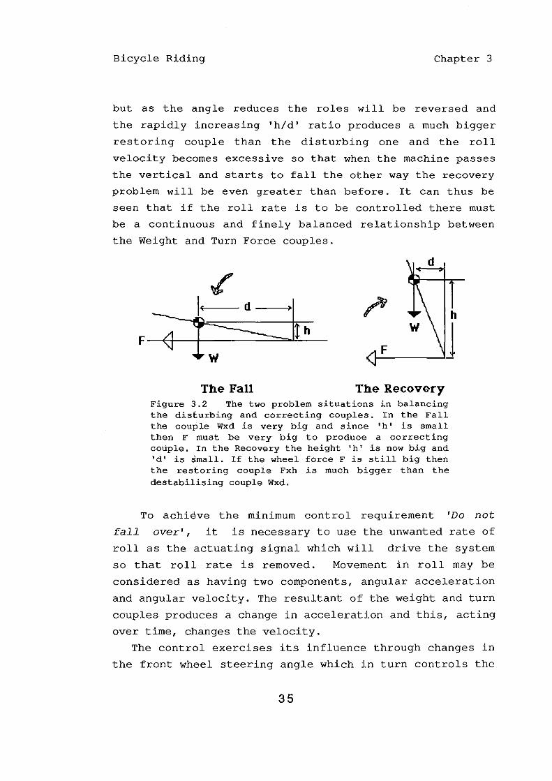
Imbalance of Couples
It can be seen from the foregoing paragraphs that
providing the bicycle is leaning into the turn the weight
couple opposes the turn force couple. However it can also
be seen that they are not well matched since the former
gets bigger with increasing lean angle whereas the latter
gets less. It is this mismatch that is at the heart of the
bicyle control problem. Figure 3.2 illustrates the problem
situations. In the first diagram, named 'The Fall', the
distance 'd' is big so the weight forms a very large
couple into the lean, but because of the exaggerated lean
'h' is small, so a very big force F would be needed to
check the fall. It must be borne in mind that not only
does this force have to match the couple formed by the
weight times the distance from the support-point (W * d)
but it must exceed it. Matching it will merely prevent
there being any further acceleration in roll but the
accumulated angular velocity, due to its having fallen
from wherever it started, must also be dissipated or it
will go on falling at that rate. During the time taken to
overcome the residual velocity the angle of lean will have
continued to increase so the imbalance situation will have
got even worse. The second figure, named 'The Recovery',
shows another problem area. Assume that the large increase
in Force has successfully contained the fall and the
machine starts to return to the upright. At first the
return will be moderate as the couples are well matched
34
Bicycle Riding Chapter 3
but as the angle reduces the roles will be reversed and
the rapidly increasing 'hid' ratio produces a much bigger
restoring couple than the disturbing one and the roll
velocity becomes excessive so that when the machine passes
the vertical and starts to fall the other way the recovery
problem will be even greater than before. It can thus be
seen that if the roll rate is to be controlled there must
be a continuous and finely balanced relationship between
the Weight and Turn Force couples.
F
~ I ~ d ~
h
lh W
J W F
The Fall The Recovery Figure 3.2 The two problem situations in balancing the disturbing and correcting couples. In the Fall the couple Wxd is very big and since 'hi is small then F must be very big to produce a correcting couple. In the Recovery the height 'hi is now big and Id' is small. If the wheel force F is still big then the restoring couple Fxh is much bigger than the destabilising couple Wxd.
To achieve the minimum control requirement 'Do not
fall over', it is necessary to use the unwanted rate of
roll as the actuating signal which will drive the system
so that roll rate is removed. Movement in roll may be
considered as having two components, angular acceleration
and angular velocity. The resultant of the weight and turn
couples produces a change in acceleration and this, acting
over time, changes the velocity.
The control exercises its influence through changes in
the front wheel steering angle which in turn controls the
35
Bicycle Riding Chapter 3
side force at the tyre/road contact point, which in turn
alters the turn couple. It has already been mentioned that
merely reducing the acceleration to zero by balancing the
roll couples is insufficient as it leaves the accumulated
velocity unaccounted for. For a minimum solution the
control must produce changes in the sideways wheel force
via the steering angle that are dependent on both the
acceleration and velocity in angular roll. This will
remove any roll movement that arises giving a constant
lean angle. Where this angle is other than vertical the
bicycle will be turning towards the lean.
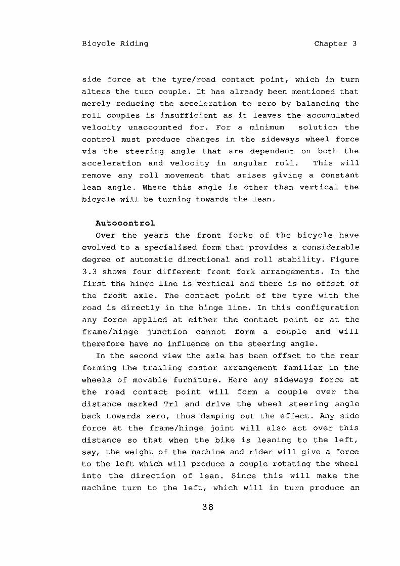
Autocontrol
Over the years the front forks of the bicycle have
evolved to a specialised form that provides a considerable
degree of automatic directional and roll stability. Figure
3.3 shows four different front fork arrangements. In the
first the hinge line is vertical and there is no offset of
the front axle. The contact point of the tyre with the
road is directly in the hinge line. In this configuration
any force applied at either the contact point or at the
frame/hinge junction cannot form a couple and will
therefore have no influence on the steering angle.
In the second view the axle has been offset to the rear
forming the trailing castor arrangement familiar in the
wheels of movable furniture. Here any sideways force at
the road contact point will form a couple over the
distance marked Trl and drive the wheel steering angle
back towards zero, thus damping out the effect. Any side
force at the frame/hinge joint will also act over this
distance so that when the bike is leaning to the left,
say, the weight of the machine and rider will give a force
to the left which will produce a couple rotating the wheel
into the direction of lean. Since this will make the
machine turn to the left, which will in turn produce an
36

Bicycle Riding Chapter 3
anti-lean couple, it is a stabilising movement in the roll
plane.
(a) No rake & no offset, (b) No rake but rearward therefore no castor. offset gives castor.
(c) Rearward rake, no offset (d) Offset axle reduces gives a large castor. the castor effect.
Figure 3.3 Showing how variation in the geometry of the front forks gives different trail distances and thus different castor effects.
When the safety bicycle replaced the ordinary or
'penny-farthing' type the rearward movement of the rider
necessitated a rearward movement of the control bar. This
was almost universally accomplished by raking the hinge
line back at an angle. Such an arrangement is seen in the
third diagram. As can be seen the effect of such a design
is a large distance between the ground-tyre contact point
and the hinge line. (Marked Trl). This gives a powerful
stabilising effect which makes it difficult to turn the
wheel out of the dead ahead when upright and produces such
37
Bicycle Riding Chapter 3
a strong couple into the lean when tilted that, if
allowed to dominate, it leads to overcompensation and a
series of wobbles from one side to the other. This is not
a desirable state of affairs for normal control and the
'stability' factor is reduced by offsetting the axle
forward to reduce the distance Trl. This dimension is
adjusted to give sufficient directional stability to
prevent stray bumps jerking the steering into dangerously
excessive angles and some
steering in the direction of
volitional movements by the
assistance in turning the
roll changes without opposing
rider. This configuration is
shown in the final diagram of fig. 3.3.
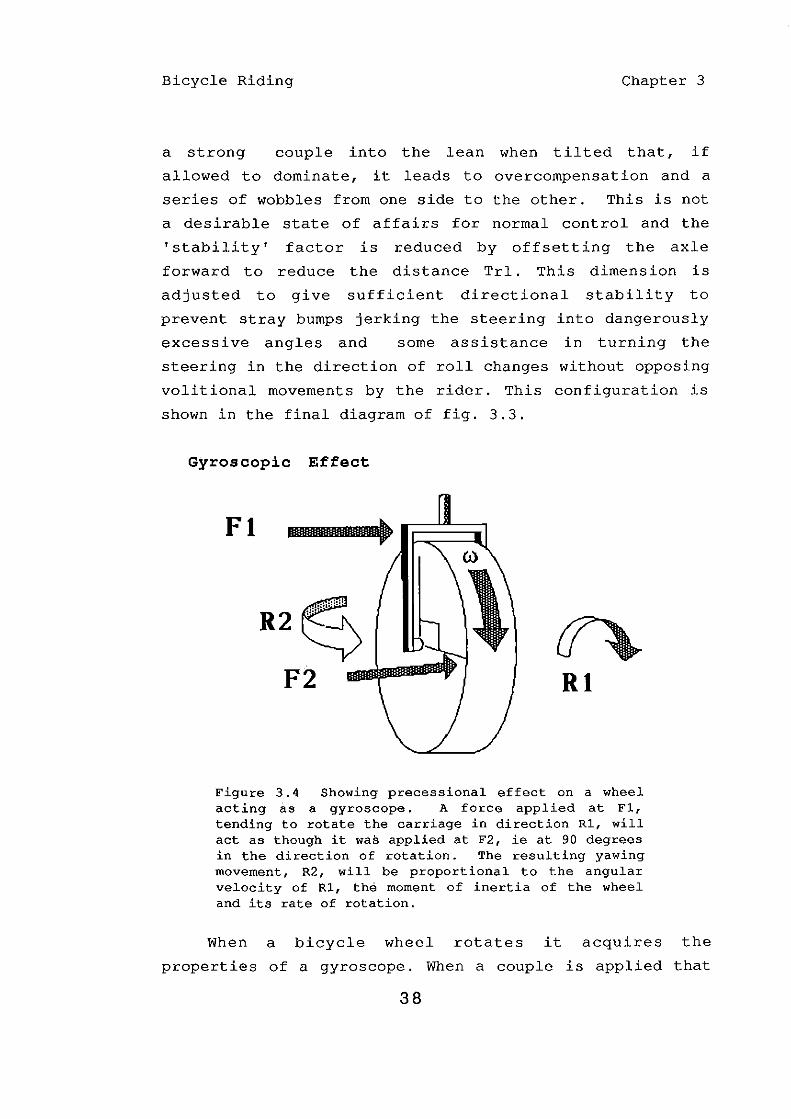
Gyroscopic Effect
FI •
R2~ F2"-!!If
n RI
Figure 3.4 Showing precessional effect on a wheel acting as a gyroscope. A force applied at FIr tending to rotate the carriage in direction RI, will act as though it was applied at F2, ie at 90 degrees in the direction of rotation. The resulting yawing movement, R2, will be proportional to the angular velocity of RI, the moment of inertia of the wheel and its rate of rotation.
When a bicycle wheel rotates it acquires the
properties of a gyroscope. When a couple is applied that
38

Bicycle Riding Chapter 3
tends to turn the wheel axle in one of the two planes at
right angles to the plane of rotation, the precessional
effect causes a turning movement in the other plane as
though the force had been applied at a point at ninety
degrees in the direction of rotation. This is shown in
fig. 3.4. The result is that any roll velocity leads to a
stabilising movement of the front wheel in the direction
of roll. The greater the mass at the periphery of the
wheel and the faster the road speed the greater is this
effect. In a small wheel bicycle at walking speeds the
effect is very slight whereas in a motorcycle travelling
at normal road speeds the effect is very powerful.
Independent and Combined Control
The autocontrol features due to front fork design
and gyroscopic effect described above provide a couple
about the steering axis. A rider who moves the steering
bar independently of this effect will feel the resultant
couple as a resistance. In a light bicycle travelling at
low speeds the effect is scarcely detectable .. At a good
road speed, say fifteen miles an hour the effect on a
normal bicycle is marked, giving a feeling of
'inevitability' to the roll stability. Removing the hands
altogether has no immediate effect. At normal road speeds
on a motorcycle the forces are so high that only a
determined effort on the part of the rider could override
the steering head couple. Thus it can be seen that two
kinds of control must be considered for bicycle control.
Whenever the steering head couple is weak the rider must
provide all the movement necessary for stable control.
When, due to front wheel size and road speed, the
machine provides a significant level of stability control
the rider need supply only those control forces required
to alter the angle of turn in the desired direction. In
doing this the rider must not apply angle dependent forces
39

Bicycle Riding Chapter 3
on the handle bar as these will interfere with the
automatic couples and autostability will be lost. What the
rider must do is to contribute a further couple which will
balance with the machine contributions to produce a
resultant which gives the desired effect. The important
point is that this couple MUST BE POSITION INDEPENDENT.
This means that the arms must move with the bar as it
alters its angle under the influence of the autocontrol
but at the same time provide a steady push in the desired
direction. In other words the force at the bar must be
independent of the steering angle. At the anatomical
level this means the rider is controlling the steering
muscles for tension independent of length. At the
experimental level it means that any record of changes in
the steering angle will contain contributions from both
the rider and the autostable effect of the front fork
design in a proportion which depends up such factors as
speed and individual design. Both the gyroscopic and
castor autostability must be removed from the experimental
bicycle if the record of handle-bar movement is to be an
unadulterated version of what the human operator is doing
but the description of how this is done will be left until
chapter 5.
The Unridable Bicycle
Before going on to consider the case of body movements
as a means of control Jones 1970 paper will be considered
in more detail now that the basic mechanics of the bicycle
have been explained. Since Jones' thesis was that a
bicycle without autostability would prove unridable it can
be inferred that he regarded the human contribution to be
of little importance. He used two tests to determine the
unridablity of the bicycles he built. One was to try and
make them travel on their own after being pushed off at a
run and the other was a subjective account of how
40
Bicycle Riding Chapter 3
difficult he found them to ride. The actual words he used
to describe the result of these latter test appear below
in italics. The first unridable bicycle (URB1) had a
second front wheel mounted alongside the first, just clear
of the ground, so it could be spun up to speed by hand
either in the same direction as the normal front wheel or
opposite to it. When it was spinning in the same direction
it enhanced the gyroscopic effect and when in opposition
it diminished or reversed it. He confessed himself puzzled
when the bicycle proved quite easy to ride at low speed in
either condition. However the effect on the bicycle
running on its own was quite clear. When the gyroscopic
force was reduced the machine fell to the ground as soon
as it was released and when the force was enhanced URBl
ran uncannily in a slow, sedate circle before bowing to
the inevitable collapse (page 36). URB2 had a 1 inch
furniture castor fitted instead of the front wheel.
Despite problems with bumps and the bearing overheating
Jones was able to ride this strange machine but was not
surprised that it would not run on its own. URB3 had the
normal front forks reversed, similar to the diagram in
figure 3.3 (b). This machine was amazingly stable on its
own, not only limiting the rate of fall but actually
righting itself and turning in the opposite direction. But
it was strangely awkward to ride, because it was too
stable and resisted control inputs from the rider.
Finally in URB4 Jones exaggerated the foreward curve of
the front forks by mounting the wheel on 4 inch extension
pieces producing a strong reverse castor effect. This
machine would not run on its own but, although very dodgy
to ride, it was not as impossible as he had hoped. The
central part of Jones' paper is taken up with deriving a
set of curves for the effect of lean angle on the castor.
This is an alternative method of working out the effective
trail distance which is dealt with in the next chapter
41

Bicycle Riding Chapter 3
using the geometrical method which Jones preferred to
avoid.
Jones had hoped that, by removing the various features
which were supposed to produce stability, he would be able
to identify the contribution each made by finding when the
bicycle became unridable. He confessed himself baffled by
his own ability to overcome the obstacles he devised. The
only modification which makes control impossible is to
lock the steering solid. Since his modifications had the
expected effect on the stability of the bicycles running
without a rider it is evident that humans can deal not
only with bicycles without any stablity but even manage
those which have been quite seriously destabilized.
A more recent study by Lowell & McKell (1981) models
some aspects of bicycle stability. The authors do not
claim this as a serious investigation of bicycle or rider
performance, but rather as a formal application of
classical mechanics to a familiar problem. In order to
keep their equations tractable they ignore both rider
inputs and gyroscopic effects which lead to some rather
strange conclusions about inherent stability which are not
born out by the behaviour of bicycles, and particularly
motor-cycles at high speeds. They quote Jones paper to
support the claim that bicycles with small castor are very
difficult to ride but in doing this they fail to
distinguish between a zero castor and a negative castor.
As will be seen later in this paper reducing the standard
castor of a normal bicycle to zero produces no handling
problems and actually gives the steering a rather pleasant
'light' feel. In any case they are misrepresenting Jones'
report since he did not make a bicycle with zero castor
and even found he could ride URB IV, with its large
negative castor.
42
Bicycle Riding Chapter 3
Lateral Weight Shift as a Control Input
Many studies have considered lateral body shift as a
possible means of control. (Lowell & McKell, 1982; Nagai,
1983; Van Lunteran & Stassen, 1967; Weir & Zellner, 1979).
Although there can be no doubt that bicycle riders do move
their upper body from side to side during riding it does
not follow that this movement is being used to control the
machine either in roll or in direction. However, it is
equally clear that rolling movements of the bicycle frame,
induced by counter movements of the riders' body, will
produce control effects via the autostability effect of
the front fork design. Roll velocity is converted by the
gyroscopic effect into a steering couple away from the
upper body lean. The resulting turn will push the centre
of mass in the direction of the initial lean. A permanent
lean to one-side will also generate a steering torque in
the same direction due to the castor effect. These effects
are confirmed by the fact that riders can control bicycles
with body movements alone when riding hands-off. As far as
this study is concerned, it is important to get this point
quite clear as the integrity of the recordings depend on
the argument that when the autostability of the bicycle is
removed body movements do not produce any significant
control inputs. What must be established is that body
movements in relation to the bicycle frame cannot in
themselves produce controlling forces independent of their
secondary effect via autostability. A preliminary
examination might suggest that an unwanted displacement of
the centre of mass to one side could be removed by leaning
the body in the opposite direction. The dynamics of the
system are, however, principally concerned with the
position of the combined centre of mass in relation to the
road support point and will be affected in a complex
manner during the movement of the rider's mass in relation
43

Bicycle Riding Chapter 3
to that of the bicycle.
(a) (b)
Figure 3.5 Despite the angle between the upper body and the bicycle frame (AL) the centre of mass, shown by the larger segmented circles, does not produce a restoring couple. Drawing (a) shows how even at quite small angles of lean a large AL fails to take the combined centre of mass onto the correcting side of the ground support point. Drawing (b) shows how, as the angle of lean approaches 90 degrees, the apparent sideways movement of the upper body produces very little change in the horizontal plane.
Exactly what happens when a rider moves his upper body
laterally depends on the relationship between the masses
of man and machine, their rate of movement and the angle
of lean.
To deal with the simplest point first let us take the
case of a rider, at some angle of lean, who has already
moved his upper body towards the vertical in an attempt to
restore the disturbance. Figure 3.5, (a) shows that there
will be some fairly small angle of lean where the lateral
44

Bicycle Riding Chapter 3
movement of the body will not put the combined centre of
mass on the restoring side of the vertical from the
support point. In such a case the movement will have
reduced the disturbing couple to the left but will not
provide a restoring couple to the right. Figure 3.5, (b)
shows that at large angles of lean the lateral movement
has a decreasing influence on the disturbing couple as the
movement lies increasingly in the vertical plane.
The above situation is static. How the rider achieves
his displaced position and what happens during the
movement have not been considered. For a start it takes
time to move from the normal riding position to the
position shown in figure 3.5, (a). During the time that
the rider is moving right in relation to the bicycle
everything will be falling left because the combined
centre of mass is displaced to the left of the support
point. This means that the angle of displacement to the
left at which the rider started to make his correcting
move will be less than the angle shown.
Given an initial displacement to one side, whether a
rider can EVER produce a correcting movement in this
manner depends on the interaction between two rates of
movement and the relative moments of inertia of the masses
moved, and this in turn depends on exactly how the rider
carries out the movement.When the rider, seated normally
on the bicycle, is displaced from the vertical so that the
centre of mass is no longer vertically above the point of
support the disturbing couple formed by the weight times
the horizontal distance of displacement produces an
accelerating roll about the support point.As the
displacement increases so does the rate of acceleration.
In order to check this movement two things are necessary.
First either a couple must be formed that will oppose the
accelerating couple or the couple must be removed. Second
an additional couple must be formed temporarily which will
45

Bicycle Riding Chapter 3
decelerate the existing roll velocity to zero at which
point it must then be removed to prevent its starting a
fall in the opposite direction. LI
~Ll
(a) Angular acceleration clockwise:-
(b) Angular acceleration clockwise:-
W * Ll I M * 10 (W * Ll I M * Io)+(F * H I (M-m) *10)
h T H
---,--1 (c) Leg movement
Figure 3.6 showing the acceleration when a limb about a narrow support details. M is total mass,
46
effect on angular is moved to balance
point. See text for 'm' is mass of arm.

Bicycle Riding Chapter 3
In the case which is being considered here the only
means the rider has of providing these couples is to alter
the relative disposition of the physical parts, such as
his limbs or torso, or the bicycle, to somehow move the
centre of mass over to the other side of the support
point. Nothing else will achieve the desired result. The
start position is shown in figure 3.6, (a). The view is
from the rear so that picture left is also left for the
rider.
If it is assumed that in the start position the rider
is sitting on the saddle then the only way he can shift
the centre of mass to the left is by moving some part of
his body in that direction. The argument is easier to
follow initially if we consider the effects of moving
first an arm and then a leg. Figure 3.6, (b) shows the
effect of rapidly pushing the left arm out to the side.
The force needed to accelerate the arm to the left will
act against the shoulders in the opposite direction. The
rate at which the arm moves is given by the force divided
by the mass of the arm (F/m) The rate at which the
remainder of the mass moves the other way is given by the
rotating couple formed by the force times the height of
the point of application above the ground (F*H) divided by
the moment of inertia about the ground contact point
(M*(h A 2)/3). Thus the effect of flinging the arm out leads
to its moving one way and the body moving the other, each
at different rates. While this is taking place the whole
is being rotated to the right under the influence of the
original couple formed by the total weight times the
lateral displacement (W*l) divided by the combined moment
of inertia «M+m) * (h A 2) 13). Thus there are two couples
driving the combined mass to the right but the movement of
the arm out to the left brings the centre of mass out to
the left with it so the lateral distance '1' is being
reduced. Because the arm is by comparison light and is
47

Bicycle Riding Chapter 3
going in a straight line it moves much quicker than the
remainder of the mass. Whether this succeeds in moving
the centre of mass onto the left hand side of the support
point before it rolls out of reach or not depends on the
actual masses and rates involved. To check the roll to the
right the centre of mass must move not just back to the
upright but beyond it in order to remove the accumulated
angular velocity to the right.
An idea of how little control is available using this
method may be gained by standing on one foot on a
laterally unstable platform, such as a rolling pin, and
trying to check an incipient fall by flinging out an arm.
It is immediately evident that the movement of the centre
of mass is not sufficient to overcome the roll. It is just
possible with care to provoke a fall towards the flung out
arm from the in-balance position but there is very little
margin for error. When a leg is moved rather than an arm
the result is more encouraging and there is certainly very
little difficulty in preventing the initial fall from
developing. It can be seen from figure 3.6, (c) that the
thrust which pushes the leg out acts much lower down. The
couple acting to the right now acts over the much reduced
distance H and consequently more of the movement will take
place at the leg. Because the leg is heavier it will have
greater influence in bringing the centre of mass back
towards the centre. Arm and
considered as candidates for
leg movements are not being
bicycle control. The only
other movement available to the seated rider is to bend at
the waist and force the upper body to one side which will
of course force the lower body and the bicycle in the
opposite direction. If the balancing act described above
is now tried using upper body lean to counter incipient
roll by leaning away from the movement the task will be
found to be impossible. In fact a careful attempt to
initiate a fall from the balanced position by a sharp
48

Bicycle Riding Chapter 3
bend in the body will show that there is if anything a
tendency to go the other way, that is the force applied
has a greater effect on the lower mass than the upper.
The masses of the two parts being moved are now more
nearly equal and the thrust is being applied well up the
body. None of these control movements has any chance of
restoring balance once the combined centre of mass has
moved more than a degree or two out of the vertical or
when there is any amount of accumulated angular velocity.
Thus we can see that although a rider can control a
bicycle entirely by moving his upper body away from a fall
this is achieved via the autocontrol effect. Even at very
small angles of lean such a movement cannot alter the
position of the centre of mass to provide a restoring
couple. A clear demonstration of this can be made by
trying to balance on a stationary bicycle using upper body
movements. Providing the chain is disconnected from the
rear wheel to prevent dynamic forces being transferred
through the front wheel this task is impossible and shows
that upper body movement on its own cannot exert control
in the rolling plane.
Indirect Lean Control
Despite the ineffectiveness of lateral body movement as
a direct means of control the automatic stability
conferred on bicycles by virtue of the front fork design
does allow lateral upper body movement to control both
roll and direction. Rolling the upper body to one side can
only be achieved by rolling the machine in the opposite
direction. This roll is converted by the gyroscopic
effect into a steering couple away from the upper body
lean. The resulting turn will push the centre of mass in
the direction of the initial upper body lean. A permanent
lean to one-side will also generate a steering torque in
the same direction due to the castor effect. Since the
49

Bicycle Riding Chapter 3
roll and turn effects achieved in this manner can be
equally achieved by handle-bar movement, and since
the movement of the handle bar is recorded on
only
the
experimental bicycle, it is preferable to avoid the
influence of upper body movements in the analysis. As has
already been mentioned above, it was necessary to remove
the autostability from the experimental bicycle to prevent
a confusion between automatic forces and human forces. By
the same token, in the absence of automatic control, any
body movements made by the subjects will not be translated
into control movements thus forcing the subjects to depend
on hand movements only for control.
The Psychological Point of View
In general the work that has been done on single track
vehicles has been in the engineering field is therefore
orientated towards vehicle design and performance leaving
virtually untouched those aspects of bicycle-riding which
interest the psychologist. Over the past thirty years a
number of engineering theories such as feedback control
and servomechanisms have been adopted by psychologists to
describe the way limbs are controlled during skilled
movements. In 1947 Craik found that people often made
corrections in aiming and tracking tasks in steps rather
than continuously and consequently described this
behaviour as an intermittent servomechanism. Keele &
Posner (1968) estimated that the minimum refractory period
was 260 msecs. Many experiments used tracking or aiming
tasks to explore control which led to a general conclusion
that there is some minimum period required for central
control to detect an error and implement a correction.
When action followed stimulus at less than this interval
it was supposed that control was via a local reflex. This
idea became so well established that the 200-250 msecs
latency was frequently taken as being the criterion for
50

Bicycle Riding Chapter 3
judging whether an action was under central control or
not. However much shorter delays than this have been
recorded in tasks where reflex control seems an inadequate
explanation. For example Cordo and Nashner (1982), whose
experiments will be dealt with in greater detail in
chapter 8, found compensatory postural movements in humans
in the latency range of 70-150 msecs which could not have
been simple reflexes since they adapted to changes in the
environment which could only have been processed
centrally. These discoveries have led to the
classification of responses into three speed categories.
The fastest spinal, or myotatic, reflex acting in the
40-50 msecs range, the centrally controlled decision range
starting at around 200 msecs and between these two there
appears to be a range of reflex like movements, known as
the Functional Stretch Reflex (FSR), which are
nevertheless under some degree of central control.
It would unwise to assume that because intermittent
control is used in some tasks that this is a general
limitation in all tasks. Whether continuous or
intermittent control is used depends initially on the
exact details and in some cases at least it is evident
that the experimental design itself forces a choice of
technique. For example both Pew (1966) and McLeod (1977)
used a tracking task in which the subjects were asked to
keep a cursor in the middle of a VDU screen. The cursor
was always accelerating at a fixed rate in a horizontal
direction and the subjects were given two keys which
selected the direction of this acceleration either left or
right. Even if the subjects had been able to detect the
rate of acceleration they had not the means to apply a
proportional correction. If the acceleration was high
when they switched directions they had to wait for it to
produce a reversal and if they switched when the
acceleration was still very small the result was a rapid
51
Bicycle Riding Chapter 3
reversal and a fast acceleration in the opposite
direction. They were therefore committed to a particular
form of control by the details of the task. In order to
test this point of view the Pew task was rewritten to
allow continuous control of the cursor acceleration with a
joy-stick. It becomes immediately apparent that an
operator can make use of the proportional response and in
its new form the task is comparatively easy. A record of
operator activity shows a continuous change rather than
the previous intermittent control.
For continuous control it is necessary first that some
variable, relevant to the reduction of error, is
detectable by the operator and second that the means of
continuous control is available. Where these two
conditions are satisfied then any delay between detection
and execution appears as a phase shift between the two
continuous movements of the actuating signal and the
manipulated variable. It is also necessary that the
subject adopts an appropriate strategy since such
variables could be detectable but ignored.
It appears from recent work with the mass-spring
theory (Kelso et al. 1980; Bizzi, 1980 & Schmidt, 1980)
that subjects in the sort of movement to a target task
used for ex,ample by Keele (1968), might be setting the
ratio of opposing muscle length/tension to achieve a final
position, in which case a continuous monitoring and
control of intermediate acceleration would not be
necessary.
Bicycle riding was selected as a naturally arising
complete skill which is so constrained that it was very
unlikely to be amenable to intermittent control at the
lowest level. Because the dynamics are non-linear it was
difficult to see how the control could be linear. The main
questions to answered were whether the control was
intermittent or continuous, which actuating signal was
52
Bicycle Riding Chapter 3
being utilized and what form the output to the manipulated
variable took. That continuous proportional responses are
within the scope of human operators was shown in a study
by McRuer and Kredel (1974) in which subjects were given
tracking tasks with varying system dynamics. When the
control device was of the non-linear acceleration form the
subjects responded by making movements which were
proportional to the rate of change of the system error,
whereas for rate control the output was proportional to
the system error itself. Regardless of the system in use
the subjects adjusted the gain so that the input to the
operator and the output from the machine were of equal
amplitude giving a system gain of 1, thus limiting the
input change to a rate which could be easily followed.
A close study of bicycle riding skill stimulates the
interest of the psychologist in a number of ways. What
exactly is the rider doing in terms of mental operations?
How can the behaviour be so flexible as to allow a rider
to move from a touring bicycle to a chopper or lOOOcc
motor-cycle without any apparent need for reshaping the
basic skill? Is everyone doing the same thing, or are
there distinctive versions of the skill?
experienced riders so
what they are doing?
two-wheel bicycles so
bad at describing
How do children
quickly? Why does
Why are even
the details of
learn to ride
convention say
that once learned, bicycle riding is never forgotten and
is this true? If the skill depends on the automatic
stability built into the front forks of all commercially
available two-wheel vehicles why could Jones ride his
grossly destabilized bicycles without having to relearn
his skill? And, central to the controversies surrounding
Schema models, how much memory and computation does such a
skill demand from the rider and to what extent is it
'ballistic' in the Schema sense of the word? The answers
to such questions depend in the first place on finding out
53

Bicycle Riding Chapter 3
exactly what body movements are necessary and sufficient
for normal bicycle control, and it is this question which
this study aims at answering.
Summary
Bicycle riding was chosen as the subject for the study
because it is acquired by many individuals and, being very
constrained by its instability, it allows only a limited
number of possible solutions. The design of bicycles
which has evolved over the years provides a degree of
autostability which varies from very little at slow speed
to considerable at high cruising speed. The high centre
of gravity and small lateral base of the rider/bicycle
combination gives a bad balance between the destabilising
and correcting couples. This severely constrains the way
in which the correcting force provided by the handle-bar
movement must be matched to the rate of roll if stability
is to be achieved. When leg and upper body movements are
ignored the freedom of movement of the rider is also
severely constrained to the single plane of the handlebar.
A record of handle bar movements and roll rate during free
riding represents the input to and output from the human
control system exercising the skill providing that they
can be isolated from the autostable design of the bicycle.
54

Bicycle Riding Chapter 4
4 • THE COMPUTER MODEL
Mathematical Modelling of the Control System
One of the ways of 'understanding' a time-series such
as the rates of roll and bar angle change during bicycle
riding is to construct a mathematical model of the
process, the model in this context being a formula which
predicts the output values from the input. The best
possible fit is obtained when the residual errors between
the predicted values and the actual values sum to zero and
are independently distributed, that is, the error value
at any point in the series carries no information about
the errors at other points, a characteristic known as
'white noise' .
The normal procedure for constructing a mathematical
model of a process is to run it without any control under
the stimulation of either a random, 'white-noise'
generator or some easily modelled function such as sine
wave oscillation. Thus the input is specified as an
experimental variable and a model which predicts the
output describes the nature of the system without control.
This is known as running the system 'open-loop'. Modern
control analysis techniques allow a very complete
specification of many natural systems in this way
including the regimes in which they are stable and
unstable and thus the sort of control systems which would
be successful in achieving stability.
There are a number of difficulties encountered in
attempting to model bicycle riding in this way. The first
is that such models are merely mathematical devices for
'joining' as it were the input values to the output and do
not necessarily mirror the actual processes under
observation. Such a model may be of great use to an
55
Bicycle Riding Chapter 4
engineer who wants to design an efficient control system
but is of less assistance to the psychologist whose aim is
to understand the human contribution in terms of mental
processes and physical movements. In the engineering world
the control system is a constructed machine and therefore
well understood, the focus of interest being on adjusting
its output so that it produces the desired performance. In
the biological world it is the control structure itself
which is being investigated and its interaction with the
rest of the structure is the means of revealing it.
The second difficulty arises out of the nature of
bicycle riding seen as a system. The 'open-loop'
requirement for the bicycle is virtually impossible to
meet because the behaviour of the machine is going to be
quite different depending on whether there is a rider
sitting on it and whether he is holding onto the
handle bars or not. Although the rider's weight could be
simulated a run would still be impossible because without
control the machine will not stay upright. It might be
possible to do very short runs under the influence of say
a short wave sine oscillation accepting a fall at the end
of each run. However the behaviour of the front wheel
assembly, essential to the machine's response, would be
quite different if free to turn than if the rider's arms
were resting passively on the bar. Since human muscle has
a resting 'tonus' or quiescent activity level, and is also
capable of reflex responses to length changes and
pressures it is virtually impossible to specify what a
'no-control' state in the rider might be.
Mathematical models of control systems are equations
showing how the variables behave in relation to each other
over time. The functions are continuous and the
introduction of either discontinuous inputs or changes
that are arbitrary or 'external' to the system invalidate
them. It was strongly suspected from the first that
56
Bicycle Riding Chapter 4
bicycle control was at least partially intermittent and it
was also seen that it would be virtually impossible to
ensure that the rider did not introduce changes during a
run which were independent of the feedback of the
bicycle's movement.
As has already been mentioned in chapter 2 existing
studies of bicycle dynamics have dealt mainly with the
problem of trying to express the stability of the
mechanical system in equation form with a minimum
contribution from the rider. In the interests of
simplicity various aspects not relevant to the particular
study were omitted. For example Van Lunteran and Stassen
(1969) ignored centrifugal forces and assumed a front fork
assembly with zero mass and Lowell and McKell (1982)
ignored both gyroscopic effects and rider inputs.
The Incremental Model
In order to meet these difficulties it was decided to
construct a discrete step model of the mechanical aspects
of the bicycle/rider unit which reproduced as nearly as
possible the responses to handle bar movement in each time
interval. The control sequence which moved the bar would
be modified to test a variety of control solutions,
including intermittent inputs. The output characteristic
would then be compared with that from a real run.
The bicycle/rider combination was broken down into
simple units and each of these was modelled independently
to determine the movement over a single discrete time
interval. The new state of each section at the end of the
interval was then used as the starting point for the
determination of the changes in the next interval. Where
there was a lack of information about performance
empirical values were taken from a real machine for the
range of speeds and angles that were of interest.
The programs for the computer simulation are printed in
57

Bicycle Riding Chapter 4
appendix 1, (a) As is common with programs which have
been developed over a period of time some of the variable
names are somewhat cryptic. In the following text
descriptions of operations will be kept as self-contained
as possible using for the most part abbreviations local to
the paragraph. When names are used which also appear in
the programs they are in single quotes except in the body
of equations where this convention is not followed to save
space on the line. BBC basic uses the % sign after a
symbol name to denote an integer. These are not shown in
the text. The simulation can model either the normal
bicycle or the experimental bicycle, which has all the
autostability removed. A full description of the latter
appears in the next chapter, but it will be referred to
from time to time in this chapter as the 'destabi1ized
bicycle' .
The programs were divided into a number of units
because of limited memory in the graphics mode. There are
several versions of the main program to accommodate
differences in control and output printing. Initial
variables for a run are set up in the program BIKE and
passed to the main program either via the data file VALS
or the BBC universal integer set, A to Z. Data specific
to the bicycle model being run are in the files BIKE_A,
BIKE B etc. These files also contain the moments of
inertia which are calculated separately in the programs
BIKEIN and MOMENTS. The details of any bike can be printed
with the routine CBIKE. The routine SCALES draws the axes
for the main program.
The input to the main program consists of changes to
the force applied to the handle bar. These are either
fully automatic or can be introduced from the keyboard.
The output takes the form of a five axis graph with
selected values, such as roll angle, velocity or
acceleration plotted vertically against time. The program
58
Bicycle Riding Chapter 4
can be stopped as required and the screen contents
printed. Many examples of the output appear in this and in
the following three chapters. It should be noted that the
names for the variables printed in these figures are
different from the names used in the computer program. The
convention followed is to use a single quote mark to
denote the first derivative of the angle, ie velocity, and
two for the second, ie acceleration. Thus, for example,
roll velocity is written as R' and steering acceleration
as SI I.
The rider/bicycle system is considered to consist of
two parts, the frame and rider as one unit and the front
wheel, forks and handle bar as the other. Within the
latter part the rotation of the front wheel was also
modelled for the precessional effects on
difference in moment of inertia of the
steering. The
frame between
having the steering straight ahead and at some large angle
is small so it is ignored. Throughout the text the
convention applies where rotation about the fore and aft
axis is called roll and that about the vertical plane,
yaw. The speed was a constant which could be altered at
the start of ~hy run. No account was taken of linear
accelerations or retardation forces.
The difficulty in modelling the movements of the
bicycle in three dimensions is finding tractable
equations. One way to circumvent this problem is to model
some limited p~rt of the action only. If, however, all
the main ingredients are to be represented then something
else has to go. In this model that something is the
strictly accurate relationship between the various
contributing forces. In the rolling plane this is not
very critical as small accumulating errors only give a
change in degree. That is,
from the steerihg angle will
in correcting for unwanted
59
insufficient contribution
lead to a 'sloppier' response
roll angle. When the two

Bicycle Riding Chapter 4
couples balance to produce zero roll velocity then the
system will be re-zeroed. In the yawing plane however the
relationship between the planes of rotation of the two
wheels and their local relative movement over the ground
is very critical as errors here can lead to a reversal of
sign which plays havoc with the turning performance.
Hence it will be seen that much greater attention has been
given to the yawing forces in the main program. The same
applies to the calculation of the effective trail distance
with changes in roll and steering angle as this is
critical for the autostable forces.
mgrav4 Mhtj mgrav3 bgrav4 S
i " IvmgraV2 I:::::;:s;I
comb.lgth
mgrav 1 ,r-1i"=~L!!..!~t&bgttav2 rake Mrad
effe!tive height bgrav 1
! ! wheel base
. • t rl (
effective length )
Figure 4.1 Showing the location of the values stored in the bicycle data files.
Rider and Bicycle Dimensions
The Triumph 20 bicycle used for the experimental runs
was dismantled, the parts measured and weighed using a
steel rule and a spring balance. The rider was regarded as
a regular vertical cylinder with no allowances made for
limb movements. The weight used for the illustrations in
60

Bicycle Riding Chapter 4
this thesis, at 11.5 stones was the mean weight of the two
subjects involved in the experiments. The centre of mass
of this cylinder was positioned 6 inches above the saddle.
The coordinates for the positions of the centres of mass
were taken from a scale drawing of the bicycle which is
reproduced in appendix 1, (b). For the calculation of the
moments of inertia the bicycle was considered to be a flat
plate with no lateral dimension. Since the wheels are
considerably lighter than the rest of the frame the
effective length and height of this plate were taken from
the 0.6 radius point of the wheels. The figure 0.6 was
taken as a compromise between the radii of gyration of a
solid disc and a wheel with all the weight at the rim, ie
0.5 and 0.7 respectively. All the above values were fed
into the file BIKE C using the routine BIKEIN.
Moments of Inertia
The rbutine MOMENTS uses the data for the specific
bicycle to calculate the moments of inertia used in the
main program and store them with the other dimensions in
the BIKE_A type files. Figure 4.1 shows the dimensions
used in this routine and table 4.1 shows the values for
the Triumph 20 bicyCle used in the experimental runs.
Where the same names are used in the following text they
appear in single quotes, except in the equations.
61

Bicycle Riding
Measurement
Wheel base Front wheel radius Rear wheel radius Effective height of bike Effective length of bike Rake angle Trail (trl) Bike mass Front wheel mass Bgravl Bgrav2 Bgrav3 Bgrav4 Man ht. Man rad. Man mass Mgrav1 Mgrav2 Mgrav3 Mgrav4 Combined mass Combined weight Combin~d C of G height Combined C of G length Bar effective length Bar mass
Moments of Inertla
Vertical about road. Vertical about C of G. Horizontal about C of G.
Program name
WB Wradl
rake trl
Mass WT RG
bar
WIO FIo RIo
Horizontal about rear wheel LIo Front wheel assembly FwIo
Value
3.28 0.85 0.85 2.79 4.26 20.0 0.15 1.0 0.1 1.39 1. 89 1.39 0.13 6.0 0.75 5.00 3.64 0.36 1.23 0.00 6.00 192.0 3.28 1.27 1. 70 0.10
84.53 20.57 2.935 12.42 0.060
Chapter 4
Units
ft ft ft ft ft degs ft slugs slugs ft ft ft ft ft ft slugs ft ft ft ft slugs lbs ft ft ft slugs
Table 4.1 The dimensions for the Triumph 20 bicycle used in the runs. These data are stored in the file BIKE_C. The moments of inertia are generated by the program MOMENTS.
62

Bicycle Riding Chapter 4
The moments of inertia about the centres of mass for
the cylinder representing the man and the plate
representing the bicycle are worked out first as follows:-
vertical Moments
man mom = man mass * ('Mrad'A2)/4 +
bike mom = bike mass * (bike ht A2)/12
Horizontal Moments
man mom = man mass * ('Mrad'A2)/2
('Mht' A2) /12
bike mom = bike mass * (bike lengthA2)/12
steering Moments
bar mom = bar mass * (bar lengthA2)/12
Fwheel mom = Fwhee1 mass * ((wheel rad * DE)A2)/4
where DE is the conversion for a wheel with its mass at
the rim to an equivalent uniform disc. (=1.4144)
The combined moments of inertia are now worked out
using the parallel axis theory. The general equation is:-
Combined mom = mom about C of Mass + (mass * (PD A2»
where PD is the separation between the axis under
consideration and a parallel axis through the centre of
mass. The various combined moments are listed with their
program names and the relevant values of PD:-
Vert. about road 'WIo' ............. 'Mgrav1 " 'Bgrav1'
Vert.about C of M 'FIo' ............. 'Mgrav2', 'Bgrav2'
Horz. about C of M 'HIo' ............. ' Mgrav3 " 'Bgrav3 '
Steering moment 'FwIo' ...... .... bar mom + Fwheel mom
63

Bicycle Riding Chapter 4
Side Force at the Wheel/Ground Contact Point
Whenever an object runs in a curve a force at right
angles to the direction of travel must be present. This
force comes from the action of the wheels running at a
slight angle to their direction of travel, dragging the
tyre over the ground. The theory governing the forces
produced at the tyre/road contact point is too complex and
incomplete to allow its use in this part of the model.
However it is evident that the general characteristic of
more angle more force holds good up to some critical angle
where the tyre stalls and the force becomes very large and
is directed almost entirely backwards as drag opposing
forward movement. It is also obvious that the force for a
given angle is dependent on the speed. It was therefore
possible to run a bicycle in a turn and, knowing the
weight of the system, the radius of turn and the speed,
calculate what the force towards the centre must be. This
method was not very precise, but all that was required was
some guidance of the size of force per wheel to ground
angle and an idea bf whether it varied directly as the
speed and angle or in some more complex relationship. Once
an approximate value was obtained it could be trimmed in
the simulation to suit a range of useful speeds.
When a bicycle runs in a steady turn the radius for the
front wheel is greater than that for the rear. This
difference in turning radius was found by measuring the
wheel tracks, allowing a reasonably accurate estimate of
the angle at which the rear wheel was dragging to produce
its contribution to the turning force. When the system is
in a steady turn the force at the front wheel must be
slightly in excess of that at the rear to maintain the
rotation but this difference was ignored in establishing
the force per wheel, that is the total force was divided
equally between the two wheels.
64

Bicycle Riding Chapter 4
The following measurements were made with a 170 lb
rider on the Triumph bicycle (weight 30 lbs). The speeds
were estimated approximately by timing the pedalling rate
for a distance of 70 yards prior to entering the turn. The
steering angles were estimated by eye against a marked
scale fixed to the frame and are very approximate. These
are not used in calculating the estimated flow angle for
the rear wheels but served to confirm the fact that
both wheels were dragging over the ground at
approximately the same local angle. The runs were made on
a newly swept sand surface and left very clear marks from
which the radii of the turns were measured with a steel
tape. Each turn was made through 360 degrees.
Speed Steer- Radius Rad.diffs Drag- Force per
angle angle wheel
(ft/sec) (degs) (ft) (ins) (degs) (lbs)
15 5-10 26 2-3 0.5 27
10 10-15 18 3-4 1 17
10 15-20 11 4-5 2 28
The last run was almost at the adhesion limit for the
tyres on the loose surface and when the turn was tightened
the radius difference increased to about 5.5" and then the
wheels slipped. The drag angles were measured from a large
scale drawing of the radii and bicycle frame and are
approximate. Because of tyre distortion under load the
relationship of force to both angle and speed is not a
simple straight line. To obtain an approximate
relationship for these two factors it is assumed that the
force increases directly with angle. If the first and last
runs are then considered it can be seen that they generate
much the same force since the larger radius turn is
performed at a higher speed. If the same angle
relationship is applied it will be seen that the speed
65

Bicycle Riding Chapter 4
factor must mUltiply the force effect by about 4. This is
very approximately equivalent to a cube function of speed.
Raising the speed to the power 2.7 gives a fairly
consistent coefficient of .03 for the three runs but is of
course very rough. However this was sufficient to guide a
choice of values for the simulation which after some
trimming was taken as speed raised to the power 1.8 with a
coefficient of 0.2.
Force drag angle(degs) * (VVA1.8) * CD
where 'VV' is the speed and 'CD' is the drag
coefficient. This keeps the system stable within the speed
range 2 to 15 mph which is all that was required.
The side-force is frictional and will therefore depend
on weight. Because the tyre is not rigid it will distort
with different loads so the exact relationship between
weight and force is not known. In order to allow for this
change the coefficient is made directly proportional to
the weight. This is established in the line:-
CD 0.0014 * WT
which must of course come before the line given above.
This gives a satisfactory performance over the weight
range 32 lbs (riderless bike) and 284 lbs (18 stone
rider) .
In reality it is obvious that there is much more to
tyre
that
behaviour than is captured here but the main point is
despite very large differences in tyre type and
riding condition all bicycles behave in approximately the
same way so exact details within those limits which allow
a stable performance are not important for the model and
did not justify a more exact measurement on the real
bicycle.
66

Bicycle Riding
Rotations
The linear
in the Horizontal Plane
speed of the machine is
Chapter 4
assumed to be
constant and no account is taken of fore and aft
retardation forces. The mass of the bicycle/rider unit
will not travel in a curve unless there is an unbalanced
force acting at right-angles to the local direction of
travel. This force must be generated by the wheels
'dragging' at an angle to their local direction of travel.
Once in a turn the relative movement between the ground
and any point on the bicycle is represented by the tangent
to the turning circle at that point. With any turning
system whether it is a car, a bicycle, a boat or a ski,
this relative angle will only be the same for all points
when they lie on a common radius. Thus ,since all such
systems are orientated normal to the radius and more or
less facing the direction of movement it follows that
there will be a difference between the local surface
movement at the front of the object and that at the back.
The controlling ratio is that of the length of the object
compared with the radius of the turn, so for a given
length the tighter the turn the greater the effect. This
difference of surface to object velocity during turning
manoeuvres is critical to the ability of all systems which
use relative surface movement to generate the turning
force, to sustain a controllable turn. Unless some angle
difference is introduced between the front and rear of the
system the increasing curvature of the flow as the turn
develops will produce an out of the turn rotating couple
which will back- off the generating angle and stop the
turn. In every controlled turn the couple rotating the
object must be exactly matched with the total force
controlling the radius of turn in such a way as to
preserve the wheel to ground angles and the forces they
67

Bicycle Riding Chapter 4
generate. It is the lack of tractable equations to
represent this situation which has led to such limited
models of bicycle performance.
Because this simulation uses a discrete step rather
than a continuous solution it is able to establish these
important angles geometrically. The principal reference is
taken as the north axis in the conventional cartographic
sense. Angles are measured as positive from north in the
westerly direction and negative in the easterly. There is
no anomaly in the southern segment as the model does not
exceed 90 degrees either side of north.
At the start of any time interval, 'Ti', each wheel
will have made some angle to the local relative ground
movement in the previous interval. Whenever this angle is
greater than zero a force at right angles to the plane of
the wheel will have been generated, the value depending on
the actual angle and the speed. During the new time
increment the combination of these two forces is regarded
as an impulse acting on the centre of mass which will then
move during the interval under both this influence and the
linear velocity which is defined as a constant. Any
difference in size or direction of the two wheel
side-forces will also cause a rotation during the
interval. The combination of the linear and rotational
movements will lead to different relative paths for the
front and rear wheel contact points which must be used to
find the new forces generated at each wheel during the new
interval. The front wheel is free to rotate in relation
to the frame so this relative movement will also produce a
couple in the steering when the ground contact point lies
anywhere but directly on the extended hinge axis. In the
normal 'autostable' bicycle this is the effective trail
distance.
its own
steering
The front wheel, having
inertia and angular
mass, will also have
velocity about the
axis which will influence the angle it makes
68

Bicycle Riding Chapter 4
with the external reference and the frame. The
precessional effect of the front wheel due to rolling
movements of the frame must also be added to this couple.
Values required in the horizontal plane
'Ti' One increment of time (10 msecs)
'VV' The linear velocity of the centre of mass.
Mass WT Mass and weight of bicycle plus rider.
'RA' Angle between local direction of travel of the
centre of mass and north.
'HA' Angle between the frame of the bicycle and north.
'SA' Angle between the front wheel plane and north.
'RSA' Angle between the front wheel plane and the
frame. (RSA is written as R in the printout figures)
'L2' Angle between the frame and the local direction
of travel at the rear wheel contact point.
'Ll' Angle between the front wheel plane and the
local direction of travel at the front wheel contact
point.
'Hw' The angular velocity of the frame.
'Sw' The angular velocity of the front wheel, forks &
bar. (Sw is written as S' in the figures)
'Roti' Angle of ground 'flow' to frame due to rotation.
'Si' Distance increment travelled by C of M in time
Ti.
'RAi,HAi,SAi' angle increments in time interval Ti.
'HwDOT,Sdot' angular accelerations of frame and front
wheel. (Sdot is written as S" in the figures)
'Fl,F2 & FF' The forces at the front and rear wheel
and their additioh.
'Trl' The effective trail distance.
The method of working out the movement of the ground
relative to the front and rear wheel contact points
(called the ground 'flow') is as follows:-
69

Bicycle Riding Chapter 4
(i) 'FI, F2 and FF' are found using 'LI and L2' from
the previous increment:-
FI= (LI * Ffac) F2=(L2 * Ffac) FF= FI + F2
where 'Ffac' is the frictional coefficient for the tyre
adjusted for speed and weight.
(ii) 'FF' is normal to the direction of travel by
definition. This disregards the difference between the
frame angle and direction of travel but is sufficiently
accurate for the shallow turns under consideration. The
error is a function of radius of turn and rear wheel
ground Ilow angle. For a 26 ft radius turn with 1.5
degrees flow angle it is just over I degree. 'FF' is
applied as an impulse over the time increment 'Ti' at
right angles to the direction 'SA', giving an angle
increment 'RAi':-
RAi ATN(FF * Ti) / (Mass * VV)
(iii) The linear advance in one time increment:
Si = VV * Ti
(iv) Any difference between the wheel forces 'FI' and
'F2' will form a couple rotating the frame. The
increment of rotation ('HAi') is found by combining this
couple with the angular velocity ('Hw') from the previous
time increment:-
HwDOT =(FI-F2) *WBI/(HIo*COS(VA) +(FIo*SIN(VA)
HAi = (Hw * Ti) + (HwDOT * (Ti A 2)*O.5
where 'HIo' and 'FIo' are the angular moments of
70
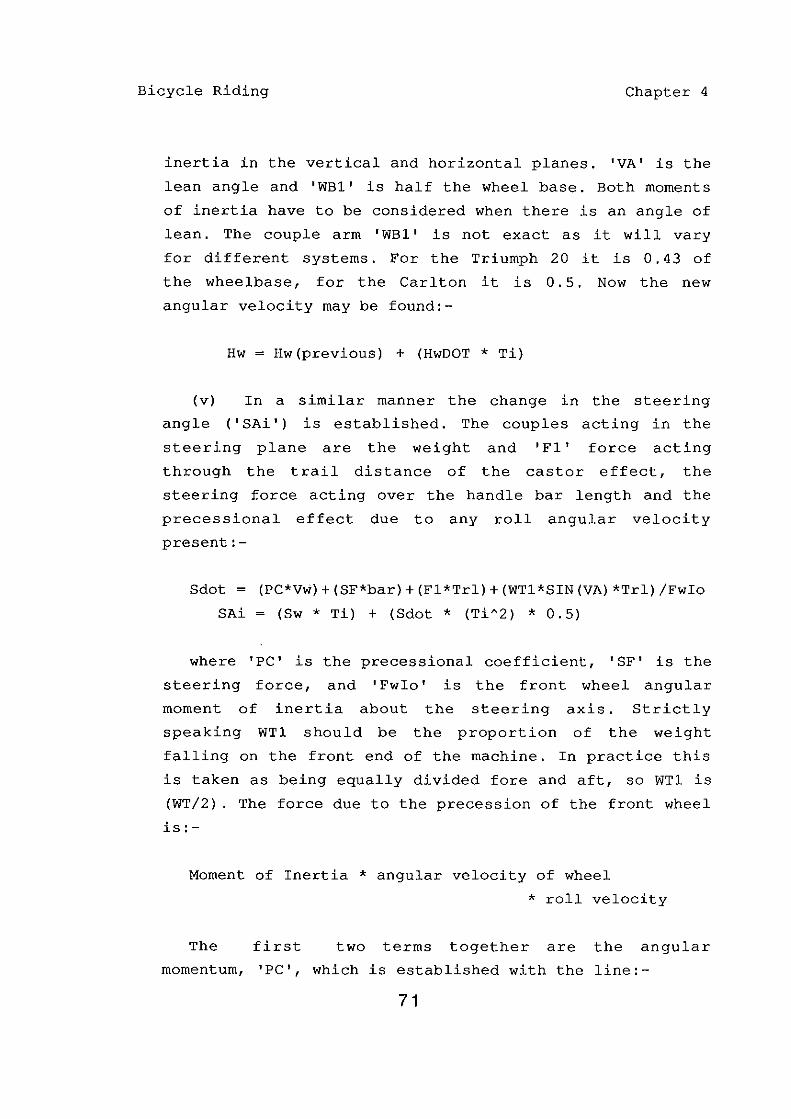
Bicycle Riding Chapter 4
inertia in the vertical and horizontal planes. 'VA' is the
lean angle and 'WBl' is half the wheel base. Both moments
of inertia have to be considered when there is an angle of
lean. The couple arm 'WBl' is not exact as it will vary
for different systems. For the Triumph 20 it is 0.43 of
the wheelbase, for the Carlton it is 0.5. Now the new
angular velocity may be found:-
Hw = Hw(previous) + (HwDOT * Ti)
(v) In a similar manner the change in the steering
angle ('SAi') is established. The couples acting in the
steering plane are the weight and 'Fl' force acting
through the trail distance of the castor effect, the
steering force acting over the handle bar length and the
precessional effect due to any roll angular velocity
present:-
Sdot = (PC*Vw)+(SF*bar)+(Fl*Trl)+(WTl*SIN(VA)*Trl)/FwIo
SAi = (Sw * Ti) + (Sdot * (Ti A 2) * 0.5)
where 'PC' is the precessional coefficient, 'SF' is the
steering force, and 'FwIo' is the front wheel angular
moment of inertia about the steering axis. Strictly
speaking WTl should be the proportion of the weight
falling on the front end of the machine. In practice this
is taken as being equally divided fore and aft, so WTl is
(WT/2). The force due to the precession of the front wheel
is:-
Moment of Inertia * angular velocity of wheel
* roll velocity
The first two terms together are the angular
momentum, 'PC', which is established with the line:-
71
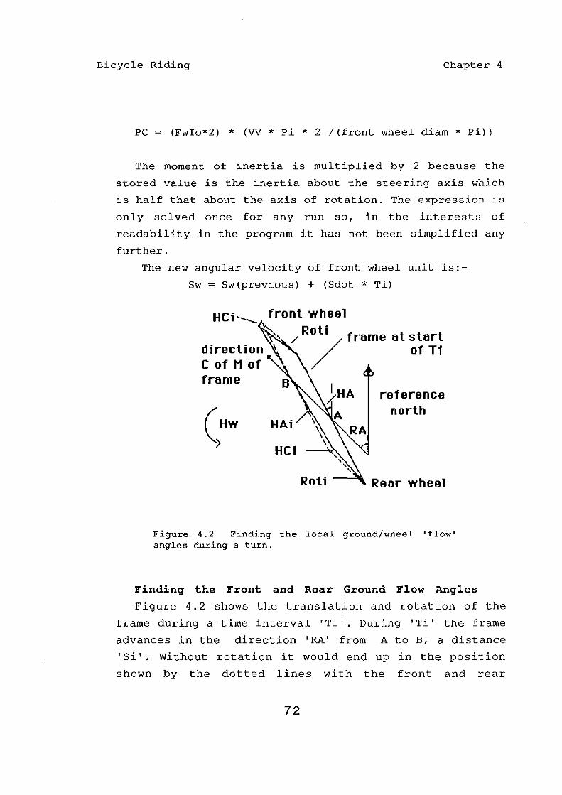
Bicycle Riding Chapter 4
PC (Fwlo*2) * (VV * pi * 2 /(front wheel diam * Pi»
The moment of inertia is multiplied by 2 because the
stored value is the inertia about the steering axis which
is half that about the axis of rotation. The expression is
only solved once for any run so, in the interests of
readability in the program it has not been simplified any
further.
The new angular velocity of front wheel unit is:
Sw = Sw(previous) + (Sdot * Ti)
HCi ........... front wheel
frame
~" / Rot i frame at start / ofTf
HAi
HCi
Roti
reference north
Rear wheel
Figure 4.2 Finding the local ground/wheel 'flow' angles during a turn.
Finding the Front and Rear Ground Flow Angles
Figure 4.2 shows the translation and rotation of the
frame during a time interval 'Ti'. During 'Ti' the frame
advances in the direction 'RA' from A to B, a distance
'Si'. without rotation it would end up
shown by the dotted lines with the
72
in the position
front and rear
Bicycle Riding Chapter 4
extremities having traced out paths with the same angles
to the direction of travel. In the situation envisaged it
is supposed that an imbalance between 'Fl' and 'F2'
rotates the frame to the left through the angle 'HAi' and
the front and rear of the frame move through the distance
marked as HCi. The ground flow at the front of the frame
alters by the angle 'Roti' so that it comes more from the
left, that is the flow angle is increased while that at
the rear is decreased by the same amount. The angles 'RA'
& 'HA' have been exaggerated in the diagram for clarity,
but for the small angles of flow normally encountered HCi
may be regarded as the common arc of the two triangles
giving the relationships:-
HCi = HAi(Rads) * half the frame length
Roti(Rads) = HCi/Si
The relationship of the ground flow at the two ends of
the frame to the external reference is:-
Front RA + Roti Rear RA - Roti
Signs of the Angles
Strict attention must be paid to the signs of the
various angles to ensure that their correct relationship
is preserved for all conditions. These are:-
'RA' positive to the left, negative to the right
'HA' positive to the left, negative to the right
'Hw' positive when rotating anti-clockwise
'Roti' takes on the sign of HCi which in turn takes the
sign of 'Hw' via 'HAi'. The other conventions adopted
are:-
73

Bicycle Riding Chapter 4
Flow Angles. positive
front of the frame
when that flow applied to the
would lead to a positive
(anti-clockwise) rotation.
Forces ('Fl,F2') positive when causing an
anti-clockwise turn.
The resulting rule for maintaining the correct
relationship at the rear wheel under all conditions is:-
L2 HA - (RA - Roti)
Since the front wheel is free to steer under the
influence of the road and bar forces its angle ('SA') must
be measured in absolute terms. Once its resulting position
for a time increment has been established then the
relative angle ('Ll') it makes with the ground flow can be
found. The sign convention here is:-
Front wheel to frame ( 'RSA' ) positive when
anti-clockwise.
Front wheel flow angle ('Ll') positive when causing an
anti-clockwise rotation.
The rule for finding 'Ll' is:-
Ll SA - (RA + Roti)
and the relative steering angle is:-
RSA SA - HA
74

Bicycle Riding Chapter 4
Order of calculating the variables
It is obvious that the exact place in the routine where
values are updated will make a difference to the outcome
and so their sequence must be chosen with care.
Variables common to several equations, such as velocity,
must be updated at the end of the period. It will be seen
in the programs AUTO and DESTAB in appendix 1, (a) lines
6000,6999 that the sequence is:-
Forces (F1,F2,FF) from previous angles (L1,L2)
Accelerations New forces, old velocities, trail & bar
force
Angle increments. New forces & accelerations, old
velocity
New flow angles Roti,L1 & L2
New velocities
New trail distance and bar force.
Rotation in the vertical Plane
Roll is influenced by two couples. First the weight
acting over the horizontal distance from the support point
of the wheels when there is an angle of lean, and second
the side fo~ce acting through the tyre contact points
acting over the vertical distance from the ground to the
centre of mass. This latter couple is exactly the same as
the centrifugal force acting over the same distance. The
way the moments of intertia interact with these two
couples
rotates
in altering the
the rider /bike
roll is complicated. The weight
combination about the ground
contact point but when the bicycle is turned to counter a
fall the action of the wheels on the ground does not pull
the centre of mass back up to a position above the contact
points but moves them in under the weight as it were. The
75
Bicycle Riding Chapter 4
equations which express this relationship do not resolve
into convenient values. For the program however the
general situation can be simply expressed in this way.
More lean means more acceleration into the fall and more
ground/wheel angle means more acceleration out of it. The
values for these couples are easy to find so the problem
rests in finding suitable values for the inertias or
viscosities of the response to them. As a simplification
of the true situation the moment of inertia used for the
weight acceleration, 'Wlo', was taken about the ground
contact point and that for the tyre-force, 'Flo', was
taken about the centre of mass. In practice this solution
works well and there was no need to trim the values.
The values used for working out the roll rate are:-
'VwDOT'
'Vw'
'VA'
'WIo'
'Flo'
'HG'
'FF I
Angular acceleration in roll (R" in figs)
Angular velocity in roll (R' in figs)
Roll angle (R in figs)
Moment of inertia about ground contact point
Moment of inertia about centre of mass
Frame height of CG above ground.
Combined side force from tyre/ground points.
The acceleration in roll is found with the line:-
VwDOT=((WT * SIN (VA) * HG) / Wlo)
+ ((FF * COS (ABS (VA)) * HG * -1) / Flo)
'FF' is the value found in the previously described
horizontal rotation section. Note the correcting couple
takes the reversed sign of this value not the lean angle.
The increment, angle and roll velocity for Ti are found
in the same way as the equivalent values in yaw:-
76

Bicycle Riding
VAi = (Vw * Ti) + (VwDOT * 0.5 * Ti A 2)
VA = VA(previous) + VAi
Vw = Vw(previous val) + (VwDOT * Ti)
Chapter 4
and the order of calculation must be adhered to.
Calculating the Effective Trail Distance
The effective trail distance is the distance from the
ground/tyre contact point of the front wheel to the
steering axis measured perpendicular to the axis, (see
figure 4.3). As the steering angle increases so this
distance reduces. For any steering angle the distance also
reduces as the angle of lean increases.
RAKE
TRAIL J " I , --1l15li/
Figure 4.3 Showing the effective trail distance in relation to the front wheel and front forks.
At varying combinations of roll and steering angle the
distance reduces to zero and then increases in the
opposite direction. At small lean and steering angles
when the distance is positive it provides part of the
autostability of the bicycle and is therefore a vital
ingredient of the model. There are three ways of
finding this distance. (1) Make selected phys ical
77

Bicycle Riding Chapter 4
measurements on a real bicycle at different steering and
lean angles. (2) Describe the front fork and frame in
space coordinates and apply the appropriate
transformations. (3) Apply spherical trigonometry. Of
these three the last is the only one which will provide an
accurate value for all combinations of angles without
taking up either too much memory or too much computation
time. The equations are complicated and would take up a
great deal of space to explain in detail, thus the final
solution only is given. The other two methods were used
to provide a table of selected values as a check on the
accuracy of the method used.
Variables External to the Subroutine
'RSA' Angle between the front wheel and the frame
'VA' Angle between the frame and the vertical
'RP' The front wheel radius
'HL' The rearward 'rake' of the steering axis
'R90' Rad of ninety degrees
'Ld' Zero angle trail distance
First the signs of the steering and roll angle are
adjusted:-
SA ABS (RSA) VA = ABS(VA) * SGN(VA) * SGN(RSA)
SD = (ATN(TAN(SA)*SIN(HL))
Some abbreviations to simplify the layout:-
CD = COS (SD) CH = COS (HL) SW = ACS(CD * CH)
78

Bicycle Riding Chapter 4
Then:-
b RP * COS {ACS [(CH-(CD*COS(SW»)
/ (SIN (SD) * SIN (SW) ) J) theta = (R90 + (VA + SD»
GA = ATN {b / (RP * -1 * TAN (theta»)
trail = {(RP * SIN (GA - SW» + Ld)
The Printed Graphs of the Simulation
With the exception of two graphs which show the output
in the horizontal for direct comparison with the actual
recordings, all the figures showing the performance of the
computer simulation take the same form. With reference to
figure 4.4, which is the first of these diagrams, it will
be seen that a brief title identifies the model and the
speed at which it is running. The output is displayed on
five vertical axes with zero time at the bottom. Seconds
are displayed in the left margin. At the top of each axis
is a bar and above this a figure in brackets which shows
the value along the X axis of half the bar. Above this is
a letter which identifies the variable running on that
axis. These are the same for all the diagrams and read,
from left to right:-
R Angle of lean (roll) in degrees
S Steering angle relative to bike frame in degrees
R" Roll angular acceleration in degrees/sec/sec
S" Steering angular acceleration in degrees/sec/sec
R' Roll angular velocity in degrees/sec
Testing the Model
With the discrete time increment method employed in
the model the changes are never absolutely accurate as
there is no feed-back between functions during the
interval. For example changes to the steering angle during
79

Bicycle Riding Chapter 4
time Ti would obviously affect the rate of frame rotation
so that the predicted change in frame angle due to the
previous wheel angles will never be quite correct.
Secs
J.
Secs
BIKE....E R
( 2)
BIKE....E R
( 2)
5 mpb S
Riderless (Destab)
( 7)
'- ]"'--'--
5 mpb S
( 7)
R·· S·· (10) (10)
Riderless (Normal) R" S"
(10) (10)
R' (5)
R' (5)
Figure 4.4 The behaviour of the simulated Triumph bicycle without a rider pushed off at a speed of 5 mph. Speed decay is not simulated. The top graph shows the destablized machine and the lower graph the normal bicycle. See text for details.
It is evident that greater accuracy could be obtained
by operating some recursive procedure which ran through
80

Bicycle Riding Chapter 4
each set of calculations a number of times trimming the
input variables on each run to get the best possible fit
between the competing contributions. However it was
decided to do without this if possible by using very small
time increments and putting up with the long computing
time. The nearer the time increments come to zero the
nearer the procedure approaches a truly continuous
relationship.
As will be seen in later chapters the model reproduces
all the general characteristics of the real bicycle. If
the bar is turned during upright running the bicycle rolls
strongly out of the turn and if then left to its own
devices the autocontrol will restore upright running.
Increase in speed increases the autostable response.
Trimming the tyre response coefficient will adjust the
amount of front wheel movement required to produce a given
lean/turn movement without altering the overall
relationship. The physical dimensions of both the rider
and the bicycle can be altered without changing the
general performance. It is even possible to put some
rather extreme bicycles into the model, such as a penny
farthing or a circus 'tower' bicycle (in which the rider
sits on the top of a six-foot tower with remote steering)
without disturbing the behaviour.
An exact correspondence between the model and the
particular bicycle chosen was not important as the
requirement was to represent the general rider/machine
situation. Any competent rider can ride any normal bicycle
without practice, and it was assumed for the purposes of
the initial model that all riders on any bicycle behave in
roughly the same way. To serve its purpose the model had
only to capture the characteristic behaviour within this
general bracket. When the time interval is too large the
system starts to overcontrol and eventually reaches a
stage of diverging osci llation. A time interval of 10
81
Bicycle Riding Chapter 4
msecs was established as the best compromise. At 20 msecs
there was some sign of instability on hard manoeuvres
and at 5 msecs, any difference was too small to show on
the screen printouts.
Two specific tests illustrate the above
Anticipating the findings of chapters 5 and 6,
points.
a delayed
control system is a more demanding test of the simulation
than the instant autocontrol of the normal bicycle. In the
first test such a system, set at a delay of 120 msecs
and the normal time interval of 10 msecs, will contain an
initial disturbance of 5 degrees of lean within 10.5
degrees of roll. If the interval is changed to 5 msecs the
performance is indistinguishable from that at 10 msecs. If
the interval is increased by a factor of four to 40 msecs
the fall is still checked at 10.5 degrees but the system
is thrown into an unstable oscillation.
The second test simulates pushing the bicycle off at a
smart trot without a rider. A normal bicycle treated in
this way will fall, slowly at first, into a turn one way
or the other. After about 4 seconds the angle becomes
extreme and the bicycle falls rapidly to the ground. The
destabilized bicycle pushed in this way falls to the
ground in about 1 second in the direction of the first
angle displacement.
The real bicycle will slow down during
whereas the simulation has no capacity for
so is slightly slower to fall. Figure
this manoeuvre
variable speed
4.4 shows the
computer printout for the two conditions described using a
launch speed of 5 mph and an initial displacement of 0.1
degrees to the left. In the first there is no autocontrol
and the bicycle falls over in about 1 sec. In the second,
with the autocontrol working, the gyroscopic and castor
effects limit the rate of fall but cannot contain it and
the bicycle eventually falls over in about 4 seconds. The
time to fall for the real bicycle when launched at a fast
82

Bicycle Riding Chapter 4
trot was about 3.5 secs. The failure of the autocontrol
to prevent the fall is mainly a function of the speed. It
will be demonstrated in chapter 7 that when the speed is
high enough the auto stability will maintain straight
running with a rider. If the simulated bicycle is
launched without a rider at 20 mph it runs true and will
recover from disturbing pushes to the handle bar. No test
of the real bike was made at this speed al though the
author heard a first-hand account from an owner who, as a
result of a bet, pushed his riderless bicycle down a steep
hill and it ran upright to the bottom.
It might be thought that changes in weight would have a
large effect on the performance but this is not so.
Because the coefficient of tyre response depends on weight
the increase in disturbing couple is matched by an
increase in tyre effectiveness which keeps the performance
more or less the same. A test of the model with different
riders gave the following responses to a fairly strong
initial disturbance of 5 degrees using the destabilized
bicycle which is a more severe test of the system:-
Wt of Rider Init. disp. Fall contained
(stones) (degs) (by. degs)
5 5 8
11. 5 5 8.9
18 5 7.6
In each case the general characteristic was exactly the
same, that is the bicycle recovered to stable running
after two or three damping oscillations though there
were of course small differences in the detail of how much
bar was used to control the movement. The exact
performance depends on how the coefficient actually alters
with weight, but for the purposes of the study the
performance resulting from the approximation was quite
83

Bicycle Riding Chapter 4
adequate.
Summary
This chapter has introduced the simulation which is
used to test various control sequences. It has avoided the
classical difficulty caused by the lack of tractable
equations by using a discrete step technique which,
although slow in operation, represents the mechanism of
free riding sufficiently accurately to predict performance
of a variety of possible control sequences. In the next
three chapters a close study is made of roll and handle
bar angles recorded during free riding. Control sequences
suggested by this work are tested on the simulation to
find their stability and whether they produce an output
characteristic which matches that of the real machine and
rider.
84

Bicycle Riding Chapter 5
5. THE CALIBRATED BICYCLE
Introduction
The main requirement was to obtain a detailed record of
the activity in the roll plane and at the steering head on
a common time base during
had been
normal free riding.
Before any recordings made it was not known
exactly which information would be of the most value so
provision was made for recording both roll and yaw rates.
It became evident that the yaw information was not needed
and since the number of recording points
any single channel depended on the
per unit time for
total number of
channels in use only the roll and handle bar channels were
used for the main runs.
Angle Change Sensors - Roll and Yaw
Either an accelerometer or a roll-rate meter will
provide the information required but the latter type of
sensor was chosen as it was cheaper and more robust. Two
Smiths Industries type 902 RGS/l Rate Gyros, were mounted
at ninety degrees to each other, one in the vertical
rolling plane and the other in the horizontal yawing
plane. No matter what the angle of lean, the roll sensor
continues to give the correct rate of change but the yaw
meter output is corrupted by any lean,
that depends on the cosine of the
giving
angle.
a response
This was
considered acceptable since the main interest was in the
roll channel and for normal riding the angles of lean were
not expected to exceed ten degrees which means the yaw
output would be within 98% of its true value. The
roll-rate meters are 'tied gyros'. A gyroscope is set in
gimbals which allow movement in the measuring plane only.
Any displacement of the gimbal from zero is detected by
85

Bicycle Riding Chapter 5
an optical sensor which then drives it back to the zero
position via a precessing current applied to a coil
winding. The current is proportional to the rate of
angular movement and this is the detected signal. The
maximum rate is 50 degrees per second which is more than
adequate for the task and the sensitivity is 60
mVolts/degree/sec. The gyros are powered by a 6 volt
accumulator carried on the bike in the instrument box.
Angle Sensor- The Handle Bar
The angle of the handle bar is read from the output of
a sensitive potentiometer geared via a rubber belt drive
to give 360 degrees of potentiometer movement for 106
degrees of bar movemeht. The potentiometer output varies
from +2.5 vdlts to -2.5 volts giving a sensitivity of
.0139 volts per degree of movement. The Zero position of
the bar and potentiometer drive were etched with two marks
that were aligned when the wheel was dead ahead. Some
difficulties were experienced at first with zero drift due
to the '0' ring drive band losing its elasticity. This was
overcome by fitting a thicker band. Zeros were measured
with a special routine during testing but since the main
interest focus sed on the rate of angle change, that is the
differential of the output, exact zeroing was not very
critical.
Speed Sensor
A perforated disc
light-sensitive cell
perforations passed
proportional to the
driven by a road wheel with a
counting the rate at which the
it, produced a voltage output
road speed. Since this device
required its own transmitting channel it was not used in
the main runs in order to improve the density of recording
points for the roll and handle bar channels. Speed was not
a critical factor and was calculated approximately from
86

Bicycle Riding Chapter 5
the length of the run and the time taken.
Transmitting the Output Voltages
Initially a radio relay link was built to transmit the
output voltages from the sensors to the microcomputer for
recording but the problems of interference between the
gyroscopes and the transmitter were never satisfactorily
overcome so a simple cable was used instead. A 5mm
diameter multicore screened cable carried the four output
voltages from the detector box on the bicycle to the
micro-computer. Losses due to cable length were found to
be negligible and the rider was unaware of the slight drag
at the rear of the machine. An 80 ft cable gave about 25
seconds of recording time for a rider travelling very
slowly in a straight line. Longer recordings were of
course possible when turning. Most of the runs were in a
more or less straight-line but no difficulties were
experienced even when several turns were made back over
the cable.
Recording the Output Voltages.
The positive and negative outputs from the gyroscopes
and steering potentiometer were converted on board the
bike to the 0-1.8 volts necessary for the Analogue to
Digital Converter (ADC) in the BBC microcomputer. The
electronics, the gyroscopes and the accumulator battery
were housed in a box that was bolted to the rear carrier
of the bicycle. The transmission wire trailed from the
rear of the box clear of the back wheel. The corrected
voltages were fed directly into the ADC port of the BBC
which was housed in a mobile laboratory with a mains
electricity supply. An assembly code routine running on
the micro read the output from the ADC channels at their
fastest conversion rate which is approximately 10
milliseconds per channel and put the raw data into a
87

Bicycle Riding
reserved memory block. The
brought the time for recording
Chapter 5
additional manipulations
one point to approximately
13 msecs plus a constant 4 msecs overhead regardless of
the number of channels in use. At the end of the run this
block was down-loaded onto disc, clearing the space for
the next run. A short binary file was also stored for
each run giving the run details associated with the raw
data file. Another program measured and recorded the zero
voltage output of the four channels as a check between
runs.
CONTROL OF THE DESTABILIZED BICYCLE
The Experimental Bicycle
A Triumph 20 inch wheel model was used for the runs.
This gave a large range of seat and handle bar adjustment,
allowing any size of subject from large adult to ten years
old child to ride with comfort. The recording box and
handle-bar potehtiometer could be easily removed and
replaced. Only the rear brake was retained because of the
bar potentiometer. The three speed gear could be altered
between runs but was normally set on low gear.
Removing the Cast(!)r & Gyroscopic Effects
The front forks of a normal bicycle are designed to
provide a measure of autostability. In order to ensure
that only the rider I s contribution to control was
recorded this stability had to be removed. Figure 5.1 and
the frontispiece
this aim.
show the alterations made to achieve
First the frame was altered to remove the rake from the
front wheel steering axis, bringing it into the
vertical. The forward throw of the axle was also removed
by mounting it on a bracket. The distance between the
88

Bicycle Riding Chapter 5
ground contact points of the wheels was not altered but
the front
axis at
point now lay directly on
all steering and lean
the extended steering
angles. With this
configuration, side forces generated during steering no
longer produce a couple in the steering head. The
handle-bar remained in
front wheel via a short
its normal position
drag link. Jones
driving the
(1970) showed
that the front wheel of a bicycle acts like a gyroscope
during riding, precessing the steering into the fall and
providing a degree of autostability. When he constructed a
bicycle with a second front wheel alongside the first and
rotated it in the
much less stable in
opposite direction the bicycle was
roll. Jones' wheel was not driven but
spun-up by hand before the run.
Figure 5.1 The destabilized bicycle, showing the front forks (OFF) without castor, trail distance nor headrake. The destabilizing wheel (DWh) is driven in the opposite direction to the front road wheel which cancels the gyroscopic effect during rolling movements. This wheel is mass balanced by a counter weight (eW).
To remove the gyroscopic effect from the experimental
bicycle a second front wheel was mounted above the primary
wheel in such a way as to be driven in the reverse
89

Bicycle Riding Chapter 5
direction but at the same speed. The tyre was removed so
that the grooved surface of the rim ran on the top of the
normal tyre and the rim was weighted to give it the same
mass distribution as the original. This arrangement put
the second wheel ahead of the centre of rotation so it was
balanced with a counter weight.
The Performance of the Zero Stability Bicycle
Although the extra wheel and the counter weight
obviously increased the inertia of the steering assembly
and the indirect operation made for a little more play
than normal, riding the Zero Stability Bicycle felt almost
exactly the same as riding the unmodified machine. This
was predictable since the autostability makes little
contribUtion to control at low riding speeds. The
steering felt light and well balanced, although the sight
of the large assembly moving during turns was a little
strange at first.
Two simple tests demonstrated that the autostability
had indeed gone. Like Jones' destabilized machines this
bike had no capacity to run on its own. If launched at a
good running speed it fell rapidly towards the side of the
first random displacement where the unmodified machine
would run on its own for several seconds. A pedestrian
pushing a normal bicycle can steer it by holding the
saddle and rolling the frame towards the desired direction
of turn. The destabilized bike could not be steered in
this manner as the wheel just kept pointing dead ahead no
matter what the operator did with the frame. It was not
possible to ride this bicycle 'no-hands', and it was
potentially dangerous as a road machine as there was no
natural tendency for the front-end to iron out sudden
directional disturbances caused by road bumps. Neither
experienced nor inexperienced riders had any difficulty
controlling this machine in ordinary manoeuvres at low
90

Bicycle Riding Chapter 5
speeds, even when blindfold.
Subjects
The runs to which this section refers were made by two
subjects. Rider A was a male subject, age 52 years,
weight 178 1bs. He was an experienced bicycle rider in
good current practice. Rider B was also a male, age
34 years, weight 147 lbs. Rider B had been a regular rider
in his youth but had not ridden a bicycle much during the
five years preceding the experiments. The two riders' leg
lengths were sufficiently similar for them to use the same
seat pillar height. This put the riders' centre of mass
some 150 mm above the seat and slightly in front of it.
The scale drawing in appendix 1. (b) shows the calculation
for the combined centre of mass for rider and bicycle.
Despite the difference in weight between the two subjects
the two centres of mass are very close together being just
in front of the saddle peak.
Method of Operation
The runs were made on a calm dry day on a sand-surfaced
hockey pitch. A mobile laboratory containing the
microcomputer was positioned on the edge of the area near
to a mains plug on an electric sub-station. The
transmitter cable was pulled out to its full length to one
side and the rider positioned at a marked start point
heading on a course leading back down the wire. The runs
passed fairly close to the recording station and were
continued beyond it taking the wire out to the other side.
The experimenter stood within reach of the microcomputer.
When ready for the run to start he called for the
subject to start and pressed the start key as soon as
the rider was stable. The program shut down after
recording 750 data points in each channel, which at 30
msecs per point is 22.5 secs. The end was signalled by a
91

Bicycle Riding Chapter 5
double beep and the experimenter called for the rider to
stop.
If it looked as though the rider would come to the end
of the wire before the automatic time was up the
run could be successfully terminated by pressing the
appropriate key. If the rider failed to stop then the
cable pulled out of its mounting without damage. The near
end of the wire was firmly anchored to prevent its
damaging the computer. Each recording period lasted
approximately 22 seconds, starting shortly after the rider
set off. All runs were started from the same place and
the approximate location where the recording terminated
was noted. Since speed was not regarded as a critical
value the approximate mean distance of the runs was
measured as 90 feet which gave an estimate of speed of 4
ft/sec Or just under 3 mph.
Blindfold Riding
At the start of the study it was evident that the
detection of roll rates is critical to the operation of
any control system. Since both the vestibular and visual
systems are capable of giving this information it was
decided to attempt blindfold riding during the recording
runs in order to reduce the number of sensory channels
being used. It turned out in practice that depriving the
rider of vision seemed to make little or no subjective
difference to the task, once the initial worry of riding
out of the prepared area was overcome. So far six people
have ridden blindfold. In each case the rider put on the
blindfold and went straight off without any difficulty.
In two cases, both children of ten, this first run was on
the destabilized model making the task that much more
exacting. Lack of time has prevented a more thorough
investigation to date, but the sureness with which all six
subjects tackled their first blindfold run argues for its
92

Bicycle Riding Chapter 5
generality. All the runs relevant to this section were
made with the subjects blindfolded.
Instructions
The subjects were instructed to ride as slowly as
possible without falling off until told to stop. There
were two reasons for opting for the lowest possible speed.
The first the restriction of the transmitting cable and
the second was the need to get as much movement in the
traces as possible. The response from the tyre when
turned out of its true track, which provides the force for
turning and therefore correcting lean, is a function of
speed.
Thus at low speed more handle bar angle is needed for
any given lean effect. The subjects were instructed to
make no special attempt to maintain direction, the
intention being to stop the run if the limit of the
wire was reached or the run came too near to the recording
van. The reason behind this instruction was that,
combined with the lack of visual information, it was hoped
that no navigational control would be added to basic
stability control during the runs. However it transpired
that, despite this instruction, subjects tended to check
developing turns unintentionally so that the general
direction of the start was maintained for the rest of the
run.
Comparing the Channel Outputs
The raw data from both channels were digital records of
the voltage output from the transducers. The roll channel
was a record of rate of angular velocity at each sample
and the bar channel was a record of angular displacement.
The sample interval was 30 msecs between each channel
point. The BBC handbook warns that although the ADC reads
to 12 bits only 10 bit accuracy should be relied on.
93

Bicycle Riding Chapter 5
Since all operations are carried out on the acceleration
information which has been smoothed twice by taking the
mean of seven local values each time it was not
considered necessary to convert the raw data. However
as a check the roll and bar values from a 600 point run
were compared with an 8 bit version. There were 264
differences out of 1200 points none of which was greater
than plus/minus 1. The bar channel lagged 15 msecs
behind the roll channel, this representing the time the
analogue digital converter takes to make a single
conversion and the program takes to store the value.
Therefore at zero LAG between the channels the bar channel
is lagging the roll channel by 15 msecs. When,
however, the handle bar data is differentiated the local
rate has been obtained by taking the change between the
target value and that value which immediately precedes it.
Consequently the differential value is in effect the mean
over the previous 30 msecs interval. The associated roll
value, which is a direct reading of angular velocity,
falls half way through this interval, with the result that
for the velocity and acceleration data the two sets of
readings are correctly synchronized and may be directly
compared without adjustment. To compare like with like
the following operations were performed.
The roll output was integrated to give roll angle.
Since the interest lay in relative changes this
integration was performed by summing the roll velocity
data without applying the time increment. This gave an
analogue of roll angle over time. During this operation
the curve was graphed so that a check could be made of the
zero position during the run. With straight runs the sum
of the roll velocities was near to zero over the total
time. Small adjustments of the DC constant value
accumulate to big changes in the final values so the zero
could be trimmed to a sUfficiently accurate figure where
94

Bicycle Riding Chapter 5
there were any anomalies. This output was then paired with
the angle data of the bar channel. In graphical studies
the amplitudes were normalized to bring the curves
together. The horizontal scale in the angle graphs has
been adjusted to allow for the 15 msecs difference between
the channel recording points.
To provide
velocities the
a comparison between the roll and bar
bar output was differentiated by taking the
change over the preceding interval and noise removed by
taking the running average of seven local values. This was
then paired with the roll data. Again the time interval
factor was not applied and in graphical presentations the
amplitudes were normalized to bring them together. These
velocity values were differentiated once more and given a
further smoothing to provide a comparison between the
acceleration channels.
Although the main argument depends principally upon
operations to the angular acceleration channels a further
smoothing and differentiation was performed to produce the
third different ial of the angle, or jerk. Much of the
detailed information is lost in this operation due to the
extra smoothing which is necessary to remove noise. Peaks
are truncated and some smaller waves are lost but the
relationship between the general trends is much easier to
see in this filtered form.
The Recorded Runs
Appendix 2. (a) shows the plots of the roll angles and
handle bar angles for twelve blindfolded runs on the
destabilized bicycle by the two subjects. Runs 25 to 30
were by rider A and runs 31 to 36 by rider M. Appendix
2. (b) shows a limited section of each run giving the
angle, angular velocity, angular acceleration and jerk for
the roll and bar (dark lines) The full runs are given as
an indication that the selected portions are
95

Bicycle Riding Chapter 5
representative of the whole. A limited section, 12 secs
of running time between point 100 and point 500, was
chosen for display so that the detail of the waves could
be more clearly seen. The start and finish of the runs
were avoided as there were possibly untypical readings
while the rider settled down to steady riding, or prepared
to stop as the wire was pulled out near to the full
length. The horizontal scale shows the recorded points
which are at 30 msecs intervals, thus the marked hundred
intervals are equivalent to 3 secs. The vertical scales
throughout have been adjusted by multiplication during the
graphing procedure to bring the peaks as near together as
possible for comparison between the rates of the two
channels.
RUN ROLL BAR
max min max min
25 0.93 -1.98 31.14 -50.52 26 1. 82 -1.21 38.11 -42.41 27 1. 27 -1.10 31.06 -47.25 28 3.66 -1.28 73.11 -22.64 29 1.0'7 -1.92 33.63 -50.28 30 2.05 -0.86 58.24 -31. 22 31 0.80 -1. 61 11.35 -46.97 32 0.66 -1. 95 14.59 -42.41 33 0.20 -1. 06 18.21 -27.72 34 0.57 -0.79 27.88 -27.28 35 1. 99 -0.68 35.98 -44.17 36 0.68 -1. 40 26.55 -47.59
Table 5.1 Maximum and m~nlmum angles of roll and bar in degrees for the destabilized runs 25 to 36.
The slow riding speed means that a large angle of
handle bar is needed to get an adequate response from the
tyres to control the roll and table 5.1 shows the maximum
and minimum angles of roll and bar used in these run
segments. It will be seen that none of the runs deviated
very much from upright running although large amounts of
96

Bicycle Riding Chapter 5
handle bar were needed to achieve this. The roll angle was
calculated from the roll rate by assuming that the
velocities applied for the duration of the interval
between samples (30 msecs) in which each was recorded, and
the resulting angle increments summed for roll angle.
General Characteristics
The activity in the first three channels of a typical
run out of the twelve under investigation is reproduced in
figure 5.2 for easy reference. For exact detai Is the
appendix printouts should be studied as the reproduction
process introduces a small degree of distortion. All the
runs show the same general characteristic. In the angle
channel, shown on the first horizontal axis, it is
possible to make out an irregular slow wave from side to
side, assuming the convention that above the zero line is
left and below is right.
The ruh in figure 5.2 has about 7 reversals of
direction between data point 100 and data point 500, a
time of 12 seconds, giving a wave period of approximately
3.5 secs. Superimposed on this slow wave is a much shorter
one which is more clearly seen in the velocity and
acceleration channels. In the example there are something
in the order of thirty reversals of direction giving a
wave period of about 0.8 secs. It is not easy to arrive at
a simple criterion which will allow a cut and dried
decision as to what distinguishes a wave from noise but an
approximate 'eyeball' count of the half-waves of both
the long and short period movement in the twelve run is
given in table 5.2. The slower wave is taken from the
angle curves and the faster from the velocity curves. The
mean number of slow half-waves for the 12 runs is 5.7,
giving approximately 0.25 hertz and the mean for the fast
waves is 23 giving 1 hertz.
97

Bicycle Riding Chapter 5
Run 33
Angleo. Roll and Bar (dark lineo)
Yeolocitlj. Roll and Bar (dark lineo)
Acceoleoration. Roll and Bar (dark line-)
Data Points
111111111111111111111111111111111111111
200 300 400
Figure 5.2 A typical section of slow straight line riding on the destabilized bicycle showing the activity in the first three channels. Reference should be made to the original computer printout in appendix 2, (b) for exact details as the copying process introduces a small amount of distortion.
The slow wave shows a tendency to a square shape with
fairly fast changes alternating with several seconds of
slow change while the differential waves have a triangular
Or • saw tooth' shape which is maintained to the third
derivative. This third derivative of angle or rate of
change of acceleration usually referred to as the jerk, is
98
Bicycle Riding Chapter 5
shown on the fourth horizontal axis in the appendix
records but has not been reproduced in figure 5.2 to save
room. In the unsmoothed form the waves show the same
triangular shape as the preceding curves but are very
noisy. The smoothing process has flattened the peaks but
it is easier to see the time relationship between the
waves in this form.
Even before the relationship between the movement in
the roll and bar channels is analysed statistically quite
a lot about the nature of the control being used can be
gleaned from a simple inspection of the traces. When
'open-loop', that is when there is no control input at
all, the bicycle/rider unit will fall at an increasing
rate of acceleration until it hits the ground.
RUN big waves small waves small/big
25 5 20 0.250 26 4 20 0.200 27 4 22 0.182 28 4 21 0.190 29 3 22 0.091 30 5 19 0.263 31 7 32 0.219 32 7 26 0.269 33 6 30 0.200 34 5 26 0.192 35 9 21 0.429 36 10 22 0.455
Means 5.7 23.4
Table 5.2 The approximate number of large and small half-waves counted between points 100 and 500 in the destabilized runs 25 to 36 with the ratio of small to big waves in the third column. See text for details.
This basic response is shown in the computer
simulation record in the upper half of figure 4.4. Because
the moment arm of the disturbing couple is constantly
99

Bicycle Riding Chapter 5
changing with the angle of lean this roll movement can
only be bought to rest by a controlling response which is
able to alter at exactly the same rate and exactly
synchronized in time. If the control system cannot achieve
this, then the next best thing is to alter at the same
rate but at some phase delay. During the delay the control
will be locally inappropriate, but providing the phase
shift is short compared to the natural frequency of
response, it will give stable control, although the nature
of the movement will be oscillatory. If the system cannot
continuously change at the same rate as the disturbing
couple the only means of control left is to change in
discrete steps. Here, at best, the controlling value will
be correct once during a discrete interval as the
disturbing couple passes through that value.
Continuous traces of the changes taking place in the
disturbing and cohtrolling couples will immediately reveal
which class of control is being used. If a discrete steps
are being used then one of the derivitive curves will show
the handle bar -trace moving in square steps while the
associated roll trace moves in a non-linear curve. That is
during the discrete interval the bar produces a fixed
acceleration or a fixed velocity while the roll angle, in
its response to the constantly changing moment arm, will
be following a changing one.
It is evident from the traces that a discrete steps are
not being used to control the roll angle and this is
confirmed later in this chapter where it is shown that the
movemeht in the bar has a very high correlation with the
local movement in the roll, but not with its own previous
movement which it obviously would have if it was using a
'ballistic' type of standard acceleration rate rather than
following the changes in roll. It is also evident that a
very short phase lag!follow system is not in use since the
acceleration is not damped down to nothing. This leaves
100
Bicycle Riding Chapter 5
the continuous follow at some moderate delay and it can
easily be seen that in all four derivitives a great deal
of the bar change is a delayed repeat of the movement in
the roll channel. The phase delay varies both between runs
and within runs but a study of the zero crossing points
shows that in run 33 in figure 5.2 the delay appears to
vary between a quarter and a half of one of the ten data
point intervals, that is between 75 and 150 msecs.
The Similarity Between the Roll and Bar Traces.
An inspection of the records for these runs shows that
the rate of movement of the handle bar is following that
of the roll at some fairly consistent time delay. The
next task is to find out how closely they are matched
and what exactly the delay is between them. It is useful
to bear in mind at this point that, with the autostability
removed from the bicycle, all movements in the handle bar
are due entirely to movements of the rider. If the rider
were to let go of the handle bar the steering would remain
at its last angle. If, as is apparent, the handle bar is
following the acceleration changes of the roll then the
rider must be making it do so.
Cross Correlation Function (CCF)
The first test of similarity between the two curves
also provides information about the delay between them.
The CCF carries out a Pearson product-moment correlation
on two columns of time series data. At each pass it varies
the 'lag' between the two columns. So for instance if a
range of lag values up to 10 was being examined, the first
pass pairs the tenth value in the first column with the
first value in the second column, then the eleventh with
the second and so on. The second pass takes the ninth with
the first and the eighth with the second and so on. This
yields a series of correlation coefficients from lag
101

Bicycle Riding Chapter 5
values of -10 to +10. If there is a similarity in the
rate of change in the two columns at some lag value the
correlation will jump to a high figure at that lag with
high correlations at the nearest lag values either side.
section Pr lag section Pr lag R sqr
RUN 1 2 3 4 5 6 7
25 100-700 .69 4 200-400 .91 4 64.9 26 100-700 .66 4 " .65 5 73.9 27 150-700 .63 4 " .64 4 74.9 26 100-700 .63 4 " .63 3 71. 1 29 100-700 .62 3 " .63 2 69.1 30 250-650 .60 4 300-500 .62 3 70.1 31 100-700 .66 2 100-300 .69 2 61. 6 32 100-700 .90 2 " .93 2 66.9 33 100-700 .64 2 " .91 2 66.6 34 100-700 .90 3 " .66 3 67.3 35 100-700 .62 3 " .67 3 76.5 36 100-700 .67 3 " .69 3 79.7
Table 5.3 Showing the correlations and lags between the roll and handle bar angular accelerations for the twelve destabilized runs (25-36) between the points indicated in column 1. See text for further details.
Short lengths of totally uncorrelated data or large
changes in phase within an otherwise highly correlated
set have a disruptive effect on the final correlation
value. Column 1 in table 5.3 shows the section of the
total ruh used to obtain the correlations in the following
column. For all but two runs the central 600 points,
representing 18 secs of running time, were used. The start
and finish sections were discarded for the reasons already
given. Run 27 and run 30 gave correlations below 0.7
for the 100-700 section and an exploration showed a sharp
increase for the more limited sections indicated so these
were used. The CCF is performed on the smoothed
acceleration data of the roll and bar channels. Limited
102
Bicycle Riding Chapter 5
sections of these data are displayed in the graphs in
appendix 2, (b). Column 2 of table 5.3 shows the Pearson
product-moment correlation coefficient obtained for each
run and col. 3 shows the lag value at which this high
figure appeared. The critical value at 0.01 probability
level even for the short set of 400 points at a lag of 50
is 0.14, so it can be seen that these correlations are all
highly statistically significant.
The MICROTAB statistical package running on a BBC B.
microcomputer was used for subsequent operations and
limited memory forced a further reduction of the data
sample to 200 points. Column 4 Table 5.3 shows the
sections selected for each run. Run 30 again proved more
choosey than its predecessors and the sample was shifted
to get a slightly better correlation. The similarity
between the correlations and lags obtained with CCFs in
the short sections and those from the full run may be
checked by comparing the values in columns 5 & 6 with
those in 2 & 3. The correlations are of the same order
but the differences in lag for rider A (runs 25 to 30)
suggest that this value is not fixed but varies to some
extent within a run. A closer look at this point will be
taken later when an alternative method of measuring lag
has been introduced.
Whether the peaks of high correlation are isolated or
appear at regular lag intervals depends on the exact
differences between the waves being considered. In the
case of exactly similar waves with constant wave-lengths
and peak a~plitudes then groups of alternatively positive
and negatitre high correlations will appear at half-wave
periods. The lag values at which the maximum peaks appear
give the phase difference between the waves. If there are
differences in wave shape within similar wave lengths,
such as a sine-wave versus a more triangular wave then the
same regular peaks of high correlations will appear but
103

Bicycle Riding Chapter 5
the peak values will be lower, reflecting the differences
in local amplitudes. In the case of exactly similar sets
of values where the wave-length and/or amplitude varies
throughout the length of the run, then the CCF gives a
much more 'focussed' response. With regular wave-length
but varying amplitude from wave to wave there is a sharp
focus of peak correlation at the critical lag value. The
positive and negative peaks still appear at half-wave
intervals but their peak correlations are much lower than
that at the correct lag value. When the wave-length
varies then the secondary peaks tend to disappear and the
peak of high correlations is confined to the critical lag
value.
totals RUN order + - zero-wave - + cols
3-7
1 2 3 4 5 6 7 8
25 1 .4 .6 .91 .5 .4 19 33 2 .4 .7 .91 .5 .3 19 32 3 .2 .6 .93 .4 .2 14 36 4 .2 .6 .89 .3 .3 14 27 5 .3 .5 .84 .4 .2 14 26 6 .3 .4 .85 .3 .3 13 34 7 .2 .6 .86 .4 0 12 28 8 .2 .5 .83 .3 .1 11 35 9 0 .6 .87 .2 0 8 31 10 0 .5 .89 .2 0 7 30 11 0 .5 .82 .1 0 6 29 12 .1 0 .83 .1 .1 3
Table 5.4 The peak correlation values either side of the absolute peak value from table 5.3, cols. 5 & 6 at half wave intervals. Thus cols. 3 & 4 are the correlations found at a full wave and one half wave preceding the peak wave respectively, and 6 & 7 are those following it. Col. 8 shows the total values of the subsidiary wave peaks (Cols. 3-7) on which the runs have been ordered. Col. 5 is correct to 2 significant figures the other columns are corrected to 1 place of decimals.
104

Bicycle Riding Chapter 5
A CCF analysis was performed for the indicated sections
of each run for a range of 24 lag values either side of
zero. The results are summarized in table 5.4. The ZERO
WAVE at column 5 shows the peak correlation obtained at
the lag value given in column 6 of table 5.3. On either
side of this are the peak values at the nearest half-wave
positions. These are given simply to 1 place of decimals
so that the eye can more easily pick out those runs which
show little evidence of peaks either side of the critical
value. The secondary peak values are summed in column 8.
These have been used to list the runs in descending order
of subsidiary peak strength. There are approximately 12
half-waves in each of the six-second run sections. From
the appearance of the CCF output it is possible to deduce
that about one third of the runs had fairly constant
half-wave periods over the six seconds run with
differences in amplitude accounting for the reduction in
correlation; a third had a good deal of disruption in
the wave period length which suppressed the secondary
waves and the final third lay somewhere between.
It looks from table 5.4 as though there is a tendency
for high correlations to be associated with high secondary
peak values. Columns 5 and 8 show a 0.616 correlation
which is significant to P<. 05 (Critical value for 10 df
0.576). The critical variables which affect the
correlation between two similar wave forms may be
considered as having two components. The first is the rate
of change of amplitude within a wave period, and the
second the half-wave period length. Since the CCF
printouts, summarized in table 5.4, show that half the
runs have considerable differences in wavelength within
the 12 secs run the question that arises is whether it is
this factor which also causes the extra reduction in peak
correlation or whether there is some unidentified factor
which affects both the wave-length and the overall
105

Bicycle Riding Chapter 5
correlation at the same time. In order to answer this it
is necessary to examine the effects of distortions in
amplitude and wave-length upon correlations in some more
detail
Effect of Amplitude and Wave-length
It is evident that two wave forms must be very similar
to obtain correlations in the order of 0.8. It is also
evident that the final figure is a consequence of the
relationship between the two values at each time point.
It would however by useful to have some general idea of
how amplitude and wave-length, as defined in the previous
paragraph, affect the final correlation.
1. Amplitude. If it assumed that there is a perfectly
consistent wave-length throughout both sets of data then
it is evident that the maximum distortion to amplitude
that cart occur within a half-wave is that one set of
values is at zero and the other somewhere near the
maximum. The following table shows the reduction in
correlation between sets of data as a result of flattening
part of one of them. The basic wave is a sine function
with 100 max. amplitude, ten 360 degree waves with a
sample rate of 18 degrees, giving 200 points. This gives
approximately 10 points to each half-wave. The second
wave is progressively flattened by setting the indicated
points at zero. The R squared term from a regression
prediction of one set of values from the other is a more
sensitive measure of similarity than correlation so both
measures are shown.
Degree of flattening Correln Regress
R sqrd
1/2 wave (1 to 10 to zero) 0.975 95.1%
3/4 wave (1 to 15 to zero) 0.952 90.6%
1 wave (1 to 20 to zero) 0.945 89.4%
106

Bicycle Riding
2 waves (1 to 36 to zero)
3 waves (1 to 55 to zero)
0.894
0.836
Chapter 5
79.9%
69.9%
This is a straight line function and does not depend
on the absolute number of waves present but the proportion
which are 'flattened'. In general terms if three out of
ten waves are at the maximum amplitude difference then a
perfect correlation will be reduced to just over 0.800.
In the case under examination the maximum correlation is
0.91 and this drops to a minimum of .83, which is the
equivalent in the table above to the difference between 2
and 3 waves set to zero, that is a change of 1/10 of total
waves. It is therefore evident that quite large
differences in wave area would be needed to account for a
reduction of this magnitude if the amplitude differences
were the only factor affecting it. Actual differences in
wave area will be dealt with shortly.
2. Wave-length. The reason that amplitude does not
have a large effect on the overall correlation is that the
disruption is confined to the locality of the associated
wave. When there are differences in wave-length, the
location of the disruption makes a big difference to the
resulting correlation. To unpack this effect the same wave
form used for the amplitude test was altered as follows;
the values in the second set of data were phase delayed by
an increasing number of degrees. For each delay value the
consequence on the correlation for the number of waves so
affected was measured. Thus if there is a phase change of
20 degrees in the fifth wave (out of a total of ten) then
half the wa~es are phase shifted 20 degrees from the other
half. If on the other hand only the last wave in the run
is shifted 20 degrees the distortion is confined to this
one position. A phase shift of 40 degrees (approximately
a fifth of a half-wave) even if applied over the maximum
of half the run only reduces the correlation to appx.
107

Bicycle Riding Chapter 5
0.94. However a shift of 180 degrees when applied over
half the run gives half at a correlation of 1.0 and half
at -1.0, and therefore gives a correlation of O. In effect
the correlation process sets the whole run at 90 degree
phase lag which gives a zero correlation. As the change
is moved down the run the consequences are mitigated but
are still strong. Just one wave 180 degrees (half a
wave) out of phase at the end of a run of ten waves will
reduce an otherwise perfect correlation to 0.8. Shortly
these differences will be examined in detail but in the
meantime a close examination of the acceleration curves
for the runs in appendix 2, (b) show that there are
frequent phase changes of about a quarter the mean
wave-length, and occasional examples of half-wave
length phase shifts. (Run 25, 450-460; run 29, 150-160;
run 30, 345-355; run 35, 390-410). Of course just how
much phase shift there is also depends on the mean lag
taken for the section of run in question and the
relationship between lag and wave-length will also be
dealt with in a later section. It is however evident that
a badly placed phase shift of this sort is sufficient to
account for the lowering of correlations noted when
selecting data runs for examination.
A more detailed discussion must be delayed until the
method of extracting a measure of wave-length and area has
been introduced. However the data summarized in table 5.4
suggests that the amplitude values are well coordinated
over time, that is the areas under the curves are closely
matched, giving a high correlation between the two wave
forms at the appropriate lag value. When the wave lengths
within the run are consistent then this leads to the high
secondary peaks at half-wave intervals shown in rows 1 to
4 of the table. When there are differences in the
wavelengths within the run the peak correlations are
reduced and the secondary peaks are suppressed. Therefore
108

Bicycle Riding Chapter 5
the expectation is that areas should show a greater
correlation between roll and bar than wave lengths and
that where there are large reductions of correlation
between roll and bar in a section of run this is due to
differences between the wavelength rather than amplitude.
Regression Analysis
To examine more closely the relationship between the
roll and bar movement a regression analysis was performed
on the acceleration data to see to what degree the roll
values predicted the bar values. For all subsequent
regressions the sections of data from point 200 to 400
were used for each run. There was considerable variation
in the lag values between runs and possibly within them as
well. The lag value from the CCF analysis, shown in
column 6 of table 5.3 was used to locate the regression
analysis. This procedure uses the equation:-
Predicted Value = Constant + (multiplier * Predictor value)
to predict a set of values from the roll data. It then
compares the predictions with the bar values at the
appropriate delay. In a series of reiterations it alters
the two injected values until the best fit is obtained.
Column 7 in Table 5.3 shows the R squared term, which
being the square of the correlation coefficient times 100,
is a measure of how well the final regression equation
fits the overall data. The minimum F value for the run
was 452. The degrees of freedom are 1 and 196 and the
critical F value for 200 degrees of freedom at a
significance of p<.OOl is 11.17. All the 't' values for
the acceleration term were in excess of 20 and the
critical value for p<.OOl for a df of 120 is 3.37. It can
be seen that the observed level of association between the
109
Bicycle Riding Chapter 5
two sets of values at the given lag is very highly
statistically significant.
Thus the analysis so far has shown that the basic form
of the rider response on the destabilized bicycle was a
close imitation of the roll rate at a mean delay between
120 to 60 msecs. The next phase in the analysis will be
to focus on the local changes in wave-lengths, delay, and
area under the curve for each wave within the runs to see
if there are any further invariant relationships in the
data.
WAVE PERIOD, AREA AND DELAY ANALYSIS
Introduction
The analysis so far has shown that the movement in the
bar acceleration channel is closely related and dependent
upon the movement in the associated roll channel. Although
the CCF analysis gives a mean delay between the channels
it is evident frdm an inspection of the graphs that there
are considerable changes in both wave period and delay
both between and within the runs. It is obvious from the
high correlations obtained that the areas under each
individual wave must be closely matched but here again
there are obvious differences. In order to find out more
about these differences a program was written which
extracted wave periods, areas and delays for the runs.
Matching the Roll and Bar Waves
The following operations were carried out on the roll
and bar acceleration waves between points 100 and 700.
Throughout the discussion the word 'wave' is used to mean
a half-wave in the convention of an alternating positive,
negative wave form.
Wave Period. The roll and bar records were each treated
as follows. The next zero crossing and direction was
110
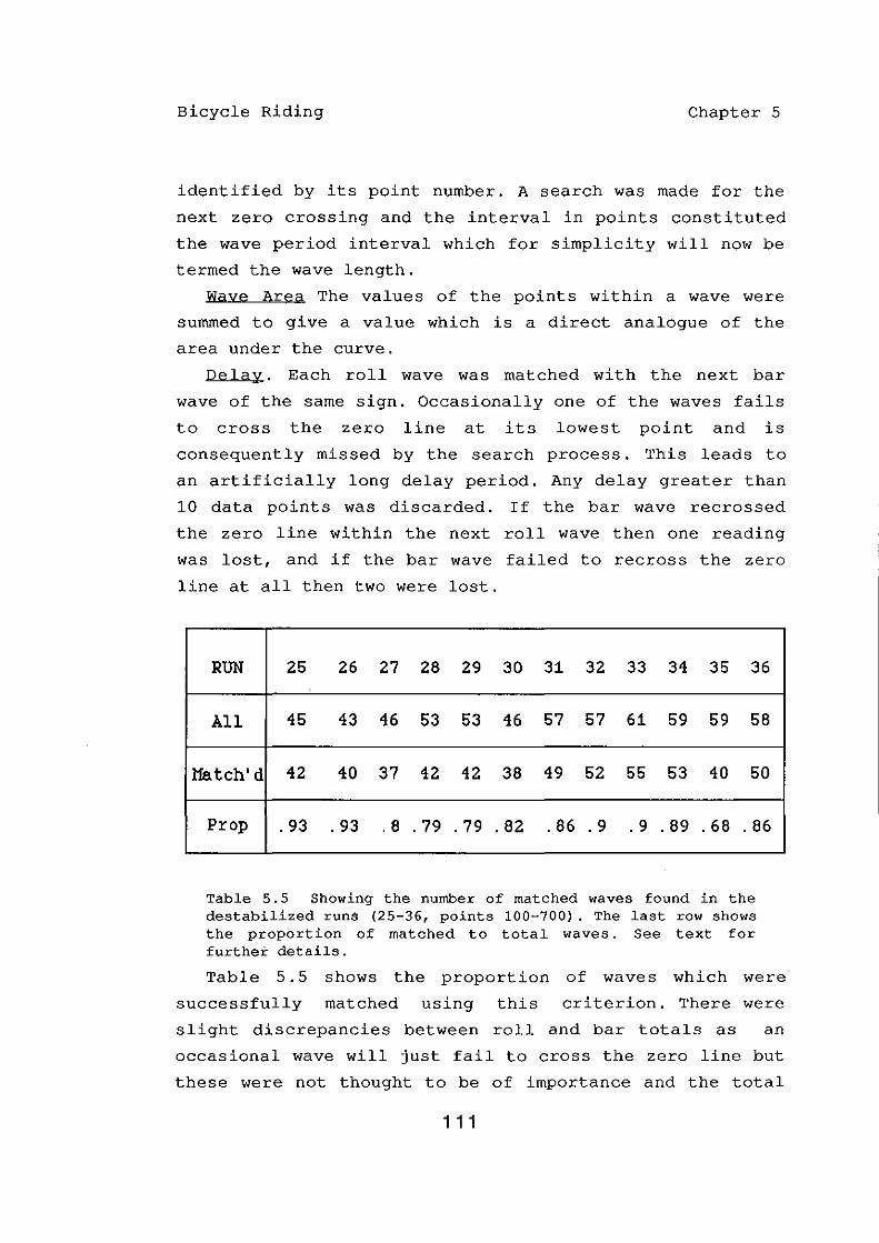
Bicycle Riding Chapter 5
identified by its point number. A search was made for the
next zero crossing and the interval in points constituted
the wave period interval which for simplicity will now be
termed the wave length.
Wave Area The values of the points within a wave were
summed to give a value which is a direct analogue of the
area under the curve.
Delay. Each roll wave was matched with the next bar
wave of the same sign. Occasionally one of the waves fails
to cross the zero line at its lowest point and is
consequently missed by the search process. This leads to
an artificially long delay period. Any delay greater than
10 data points was discarded. If the bar wave recrossed
the zero line within the next roll wave then one reading
was lost, and if the bar wave failed to recross the zero
line at all then two were lost.
RUN 25 26 27 28 29 30 31 32 33 34 35 36
All 45 43 46 53 53 46 57 57 61 59 59 58
l1atch'd 42 40 37 42 42 38 49 52 55 53 40 50
Prop .93 .93 .8 .79 .79 .82 .86 .9 . 9 . 89 . 68 . 86
Table 5.5 Showing the number of matched waves found in the destabilized runs (25-36, points 100-700). The last row shows the proportion of matched to total waves. See text for further details.
Table 5.5 shows the proportion of waves which were
successfully matched using this criterion. There were
slight discrepancies between roll and bar totals as an
occasional wave will just fail to cross the zero line but
these were not thought to be of importance and the total
111

Bicycle Riding Chapter 5
wave figure refers to roll waves only. From this it was
concluded that the matched waves were representative of
the activity in the two channels and the analysis
proceeded on these waves.
Internal Consistency
The first question to be answered is how consistent are
the measures within the runs. Table 5.6 shows the mean
values for wave, area and lag for the 12 runs. (cols.
1,3,5,6,9) .
wave-period wave-area 1ag
RUNS roll bar roll bar
1 2 3 4 5 6 7 6 9 10
25 14 4B 12 4B 122 77 115 BO 4.5 4B 26 14 42 13 4B 120 67 9B BO 4.0 62 27 15 37 13 49 146 63 13B 75 4.1 51 2B 13 35 12 40 112 5B 109 63 4.0 52 29 13 44 12 42 96 70 B6 74 3.6 57 30 14 3B 13 46 106 70 101 64 4.3 53 31 14 53 10 46 115 72 79 67 2.9 54 32 11 42 10 40 105 65 B6 66 2.9 41 33 11 44 10 44 103 92 90 77 2.9 45 34 10 3B 10 36 105 66 104 66 3.6 3B 35 13 39 12 56 141 73 132 Bl 4.1 4B 36 11 42 11 43 117 72 100 71 3.9 4B
means 13 42 11 45 116 70 103 72 3.7 50
Table 5.6 Showing the values and variability for the half-wave periods, wave areas and lags for the 12 destabilized runs 25-36 (points 100-500). The even columns show the coefficient of variation (stand. dev./mean * 100) for the value in the preceding (odd) column. Each value is the mean for the run. All but column 9 are corrected to the nearest whole number. Column 9 is corrected to 1 place of decimals.
The even numbered columns show the coefficients of
variation. This is the standard deviation divided by
the run mean and, being independent of the absolute
112

Bicycle Riding Chapter 5
values, may be used to compare the amount of variability
for all measures. These values should be read in
conjunction with the histograms of the actual scores given
in appendix 2, (c) .
Waves Areas Autocorrelation roll/bar roll/bar Bar Bar Roll
Corrn. sig Corrn. sig. wave a.rea. area
RUN 1 2 3 4 5 6 7
25 .44 .01 .80 .01 ns .62 .42 26 .37 .05 .85 .49 .37 27 .38 .05 .54 ns .57 28 .56 .01 .63 .34 ns 29 .42 .80 ns .46 30 .84 .69 .43 .37 31 .71 .80 ns .31 32 .72 .80 ns .36 33 .82 .90 .35 .53 .50 34 .51 .82 " .55 .48 35 .44 .74 " .46 .44 36 .48 .82 " ns ns
means .p6 .77
Table 5.7 Showing the roll/bar correlations and autocorrelations for wave-period and area. Columns 2 & 4 show the significance level for the correlation in the preceding column. In columns 5-7 the coefficient is shown only if it is significant at better than the P<.05 level.
Because of the row limit in MTAB these have been shown
separately for the two individual riders but they give a
clear illustration of the point that the wavelengths are
much closer to the means than the areas which have a
square distribution. This is reflected in the coefficient
of variance being nearly double for the latter. The lag
shows a similar characteristic to the wavelength.
113
Bicycle Riding Chapter 5
Relationship Between Roll and Bar
Since the correlations and regressions have shown that
there is a close relationship between the roll and bar
movement the next question is how the local changes in
wavelength and area are correlated between the roll and
bar.
Table 5.7 shows that there are significant correlations
between both sets of values but that the area is the more
closely correlated of the two. Thus a situation exists in
which there is a tendency for the wavelength to vary to a
lesser degree about a single value but when changes do
occur they are only moderately correlated between the roll
and bar channels, (col. 1).
The areas of successive waves on the other hand show
almost twice as much variation as the wavelength and
have a square shaped distribution showing that anyone of
the range of values is as likely to appear as another. As
these changes take place they are highly correlated
between the roll and bar. Column 3 shows that 8 out of the
12 runs have a correlation of over 0.8 with a mean for all
areas and many
followed by a
runs of 0.77. Thus there are many small
large areas and a small tends to be
matching small and a large by a large. Wavelengths tend
to vary about one size and where there are differences
a small one is less frequently followed by another small
one. The delay between the channels also shows a tendency
to be distributed around a single value and the variation
is of the same order as the wavelength. The mean values of
lag extracted by the measuring process for each run can be
checked against the lags resulting from the CCF analysis
by comparing column 9, table 5.6 with column 3, table 5.3.
In general the former are slightly higher than the latter
but it should be borne in mind that they are measured
exclusively at the zero crossing position whereas the CCF
114
Bicycle Riding Chapter 5
is taking the best interval for all parts of the curve.
Because the minimum interval is 30 msecs this is in any
case a rather coarse measure, giving discrete jumps to
represent a process that must certainly be continuous.
The only dimension the rider can alter is the rate of
bar movement. However the way in which it is altered can
take several forms. First the length of the delay between
the sensed roll rate and the bar rate output can alter.
Rapid changes in the delay are bound to lead to local
changes in wavelength. The amount of response, or gain,
can be altered. If the rate is held at zero for example
for a short time then there will be associated changes in
the local wavelength which will lead to changes in delay
measured at the zero crossing points. The same thing will
happen if the gain is rapidly increased or decreased and
very similar effects will follow the superimposition of
bar rates that are independent of the basic follow rate.
A more detailed analysis of whether these changes are
noise caused by the system's inability to sustain a
constant value for lag or gain and how they affect the
characteristic follows in the next chapter. However one
more question can be answered at this stage and that is
whether there are any signs of these changes being
ballistic in nature.
Evidence for Ballistic Control
The recorded roll and bar rates show that the system
is operating continuously and not in discrete steps.
However it might be asked whether it produces, for
example, a standard wavelength or delay which achieves a
partial solution to the immediate control problem and then
gradually shifts this value on the basis of feedback of
errors between the desired state and the state actually
achieved. If any of the values showed this sort of change
then there would be an autocorrelation with neighbouring
115

Bicycle Riding Chapter 5
values within the run.
The autocorrelation process performs a series of
correlations between a time series and the same series
shifted by a lag value. The first pass compares point 1
with point 2, point 2 with point 3 etc. The second pass
compares 1 with point 3 and 2 with 4. If there is any
tendency in the run for neighbouring values to be more
like each other than more remote values the correlation
will be high at a lag value of 1 and perhaps 2.
The delay value can be dismissed quickly as there were
no significant correlations between one value and
neighbouring values up to a lag of 8 for any of the 12
runs. Column 5 of table 5.7 shows that there was only one
significant correlation at a lag of 1 for the bar
wavelengths and none at a 1ag of 2. Thus it is clear that
there is no 'ballistic' tendency in the wavelength.
Column 6 shows that 7 of the 12 runs showed a moderate
degree of correlation between immediate neighbouring
values (lag of 1) of the bar areas. There were no
significant correlations for the second lag position.
Since the bar area is highly correlated with roll area
(Col. 3) it would be expected that when for some external
reason two adjacent roll areas are similar then the bar
area would show the same tendency. Of the seven runs with
a significant correlation at 1 lag, six show a significant
correlation at 1 lag in the roll data. It can be
concluded that
unlikely in
any sort of ballistic control is very
the bar area since five runs showed no
similarity in adjacent values but displayed general
characteristics of control no different from the other
seven runs. Since run 28 showed a significant correlation
in the bar area at 1 lag without there being a similar
correlation in the roll area the appearance of such a
correlation cannot be due exclusively to the observed
tendency for the bar area to copy the roll area. In
116

Bicycle Riding Chapter 5
general it appears that the dynamics of the system as a
whole are such that there is a tendency for roll areas to
show some degree of autocorrelation and that since the bar
area is closely associated with the roll area this is
reflected by a lesser degree of autocorrelation in the bar
areas.
Summary of Basic Run Output
Two subjects rode the destabilized bicycle,
blindfolded, for six runs each of just over 20 seconds.
Although instructed not to correct for any turns they did
in fact keep the bicycle oscillating about the upright,
reversing incipient falls about once every two seconds.
This was not achieved smoothly as there was a short wave
oscillation of roll of about 1 hertz. Because of the low
speed large amounts of bar movement were needed to control
the roll but the analysis is concerned with the rates of
change rather than absolute values. Because all
autostability had been removed from the bicycle all the
bar movement must have been due solely to rider response.
The form of this response was a close imitation of the
roll rate at a delay which varied from 4 to 2 data
points (120 to 60 msecs), measured by the mean delay given
in the CCF analysis. A regression analysis showed that
from 70% to 86% of the bar movement was accounted for by
the movement in the roll channel. The 1 hertz wave
component was isolated in the acceleration waves at the
zero crossing points and waves with same signs matched.
Each pair of waves yielded measures of lag/delay, local
half-wavelength period and area under the curve. Lag and
wavelength showed a coefficient of variation of 40/50
about a mean value with the roll and bar channels
correlating at about the 0.55 level. The areas on the
other hand showed a coefficient of variation of 70 with a
fairly even distribution between the maximum and minimum
117

Bicycle Riding Chapter 5
values. The matched wave areas showed a correlation at
about the 0.77 level. It was evident that the system was
detecting the roll changes continuously not at discrete
intervals and there was no tendency for the bar responses
to be 'ballistic'.
The first part of the analysis has shown that, although
each run had a completely different sequence of values in
the two channels, an invariant relationship between the
activity in the roll and bar rates existed. The handle bar
angle responded continuously to the changes in roll rate,
which since the riders were blindfolded must have
originated in the vestibular system. The delay between
detection and response was considerably faster than that
traditionally associated with central decision making and
is therefore in the range associated with the functional
stretch reflex. The next stage will be to find how such a
response affects the performance of the rider/machine and
whether that part of the bar activity which is not
accounted for by the roll activity is noise or some
additional means of control.
118

Bicycle Riding Chapter 6
6. SIMULATING THE DESTABILIZED BICYCLE CONTROL
Testing the Implied Control System
In the previous chapter it was discovered that a large
part of the activity in the handle bar acceleration
channel during normal straight running on the bicycle was
accounted for by the movement taking place in the roll
acceleration channel some 100 msecs earlier. The next step
in the analysis is to put this kind of control into the
simulation to see what performance characteristic results.
This output will be compared with that of the actual runs
and modifications sought which will bring the two nearer
together. The final aim will be to try to construct a
control system for the model which gives an output with
the same characteristic as that of a real rider over a
comparative run time.
The General Response to Delay/Follow control
Moving the bar to the left forces a roll to the right
so that a rising roll value is suppressed by the rising
bar that follows it at the lag interval. It can thus be
appreciated that the effect of the delay in the bar leads
to a situation at every peak where the bar is still
increasing even though the roll has already been forced to
reverse. During this interval the bar, having checked the
roll increase in the initial direction, is now driving it
the opposite way. Thus when the bar follows the roll at a
delay there are two opposite effects. It reduces the roll
acceleration when it is in the same direction and
increases it when it is in the opposite direction. Which
of these effects dominates depends on the combination of
two factors, first the length of the delay and second the
degree to which the bar value responds to the roll value.
If the delay is very short indeed then the bar movement is
almost all used in containing the roll and the roll
119

Bicycle Riding Chapter 6
divergences are damped out rapidly to zero. In this case
the higher the multiplication factor the quicker the
damping. The limit case in the opposite direction is
when the delay is as long as the time taken for the
bicycle to fall all the way to the ground, say 2 seconds.
In this situation the bar movement would fail to reduce
the roll at all, regardless of the mUltiplication factor.
However there is in practice a much shorter limit period.
Even if the delay is substantially less than that
given above and the bar movement manages to contain the
fall by virtue of a high multiplication factor, this same
high factor will then force the roll in the opposite
direction during the lag period. On the reverse it will be
faced with a much worse condition as the bicycle will now
be falling the other way at a speed that is the
combination of both the gravity effect and the velocity it
acquired during the reverse thrust.
Consequently it can be seen that with a lag/follow
system the gaih factor must be matched to the delay
period so that with a long delay a high gain does not
drive the system into diverging
also an absolute upper limit for
oscillations. There is
lag where even a weak
gain factor will fail to reverse a roll divergence. There
must also be some minimum delay period that is dictated by
the time taken for the physiological mechanism to extract
the information, process it, transmit it to the operating
muscles and for those muscles to respond. In the
previous chapter the lag for the two riders, measured at
the zero line; was seen to vary about a mean of
approximately 100 msecs with occasional values near to
zero or greater than 200 msecs. The first question to be
answered is what is the general response characteristic of
the simulated bicycle to variations in lag and gain in a
delay/follow system.
120

Bicycle Riding Chapter 6
Stability
The output of a system proposed for the rider/bicycle
combination has two principal parts, one a steady state
component directly related to the input and the other made
up of transient terms which are either exponential or
oscillatory with an envelope of exponential form.
time
(8) ( b)
(c) o (d) (e) Figure 6.1 The feedback control actual value and
five kinds of stability common to systems. The difference between the the desired value is used to drive
the initial disturbance back to the zero line. The ratio of the control force to the damping dictates whether the system is stable or unstable.
(a) Under-damped; stable oscillatory. (b) Under-damped; unstable oscillatory. (c) Under-damped; 'just stable'. (d) Over damped. (e) Critical damping.
Damping in the system suppresses these transient
effects and the way it behaves as a result is described as
follows. If the exponentials decay to zero the system is
said to be stable. If any exponential increases, the
system is said to be unstable and a theoretically 'just
stable' system shows a sinusoidal oscillation with a
stable amplitude. Figures 6.1, (a), (b) & (c) show an
121
Bicycle Riding Chapter 6
example of each case. If these transients are too
heavily damped the steady state component may fail to
reach the controlling value in which case the system is
said to be overdamped. When the damping is such that the
new value is reached rapidly without oscillation the
system is said to be critically damped. Figures 6.1, (d) &
(e) show these last two conditions. Since the term
'critically damped' has a precise definition the term
'dead-beat' will be used to describe a condition which
nearly approaches the critical state. Appendix 3, (a) shows
the four main cases on the simulator using the
destabilized Triumph with a 160lb rider at 4 mph using the
delayed roll/follow control with a lag of 120 msecs.
Although only the repeat of the roll acceleration has been
discussed so far the latter part of this chapter has been
anticipated in constructing these diagrams in that the bar
channel is a repeat of a combination of both the
acceleration and velocity roll channels for reasons which
will shortly become evident.
It would be convenient at this stage to have some
quantitative measure of stability with which to describe
the effects of gain and lag. The normal engineering
control procedure for describing the stability and the
suitability of proposed control for a system is to work
from the op~n-Ioop data to the closed-loop performance.
The open-loop equation of the system in the Laplace form
is graphed on a Nyquist diagram which plots the real terms
on the X axis and the imaginary on the Y axis. From this
diagram it is possible to predict what time and gain
constants will produce a stable closed-loop system.
The quantitative measures of stability are the gain and
phase margin which are defined as follows
(Healey,1967,pages 102-117)
Gain margin. That increase in open-loop gain which
gives an overall gain at 180 degrees phase shift of unity.
122

Bicycle Riding Chapter 6
At this point the system is on the verge of instability. A
negative gain margin indicates an unstable system.
su.
600
500
400
300
200 over,.. damped Fails to reaoh oontrol value too stable
100
critical.l.:r S'fA.BILI'fY da.ped
D
e
B
A.
just stahl.e
Destabilised Tri\lJl\ph
Normal Corsair
u nde r - da m I!ed Diverging osoillatory unstable
Figure 6.2 The upper and lower stability limits for two different 1bicycles' running on the simulator. The dark lines show the gain settings associated with these two points for the Triumph 20 destabilized machine at 200,150,100 and 50 msecs lag, identified by the dark lines A,B,e and D respectively. The same points for the Carlton Corsair tourer are shown by the light lines a,b,c and d. The speed is 4 mph and the rider dimensions 6ft and 5 slugs (16Ubs).
Phase margin. That phase lag required to put the
system on the verge of instability with the existing gain
value. If the system is already unstable this value will
be negative. In the absence of open-loop data no single
quantitative measure for the stability can be given.
However an idea of the stability performance of the total
system running with the repeat/delay control can be
obtained by identifying the two points where the system
changes characteristic from underdamped to over-damped and
123
Bicycle Riding Chapter 6
from stable oscillatory to unstable oscillatory for a
range of the critical variables gain and lag. Figure 6.2
shows in graphic form these two points for a range of gain
and lag values.The function of the stability between these
points is continuous and would appear on a Nyquist diagram
as a spiral. Because no values for the stability are
available here the two points are merely joined with a
straight line to aid identification. The two boundary
conditions were obtained by gradually increasing the gain
setting until the trace showed the required
characteristic. For the 'Critical damping' case (Appendix
3, (a), first figure) the gain setting was that which
.caused the velocity trace (R') to just reach the Y=O axis
but not cross it. For the 'Just stable' case (Appendix
3, (a), third figure) the gain setting was that which gave
no change in amplitude (measured in the acceleration
channel, R") over time.
The two points enclose the range of useful stability.
For any given lag when the gain is low the stability is
good but the power to control disturbances is poor. As
the gain is increased to give more power the system
approaches the point of unstable diverging oscillation.
When the lag is long only small gain values are possible,
and as the lag gets shorter so more and more gain can be
used without sending the system into the unstable range.
The lag and gain are the critical variables for any
given system, other variables having little effect on the
stability performance. Different bicycles constitute
different systems with different stability
characteristics. To illustrate this point the stability
range for two machines is shown. The dark lines show the
stability for the Triumph experimental bicycle and the
light lines the stability of a large wheeled touring
bicycle (Carlton Corsair). The bicycle speed and rider
dimensions are the same in both cases. It is evident that
124

Bicycle Riding Chapter 6
the design of the tourer is superior to the small wheel
utility machine allowing more gain to be used for the same
lag.
Changes of non-critical values within a single system
do not have
this point
(weight and
much effect on the stability. To illustrate
the effect of a range of rider dimensions
for the two
height) and road speeds
stability points for
on the gain
the Triumph
running at 100 msecs lag are shown:-
Speed 4 mph. Lag 100 msces.
Wt Ht Stability Gain stones ft
18 6 Critical 100
Just stable 265
11 6 Critical 100
Just stable 265
5 4 Critical 110
Just stable 200
settings
bicycle
Table 6.1 The effect of rider weight and height on the upper and lower stability boundaries. Taken from runs on the simulated destabilized bicycle.
It can be seen from this table that large changes in
rider weight and size have very little effect on the
stability boundaries of the system. As already mentioned
in chapter five the response from the tyres which
provides the controlling couple is a frictional force
which is dependent on the weight. The heavier the rider
the more power per angle of drag is available for
countering the weight disturbance so there is in fact not
a great deal of difference in the amount of gain
between light and heavy riders. However, even
125
required
if this

Bicycle Riding Chapter 6
were not so, it would not change the stability boundaries.
It would merely mean that, for a given lag, a heavy rider
would reach the diverging oscillatory condition sooner
than a light rider, not that the threshold was different.
Rider 11 stone 6ft. Lag 100 m.secs
Speed Stability Gain m.ph
2 Critical 110 Just stable 275
4 Critical 100 Just stable 265
6 Critical 115 Just stable 250
10 Critical 115 Just stable 230
Table 6.2 The effect of speed on the upper and lower stability boundaries. Taken from runs on the simulated destabilized bicycle.
The response from the tyres is dependent on speed. Thus
more tyre/road angle is needed to counter a given lean
angle as the speed decreases which means that mOre gain is
needed for a fixed lag when manoeuvring at low speed.
However the gain margins are not much changed by speed
so that the system will be more oscillatory at low speed
because it is forced to operate at a higher gain setting
and thus nearer the 'just stable' boundary and not because
the stability characteristic has altered.
Power for Control and Wavelength.
In general the greater the gain the greater is the
instability and the lower the gain the lower is the power
of response. All control systems are a compromise between
126

Bicycle Riding Chapter 6
these two opposing requirements. There are two unstable
conditions, one when the gain is so low that the system
cannot correct a disturbance and the other when the gain
is so high that the system takes on a diverging
oscillation. Regardless of where the stability margins lie
the control needs the power to deal with disturbances and
this is a function of absolute gain. As the angle of lean
increases so does the disturbing couple and the rate of
fall increases exponentially. The correcting couple must
accelerate faster in order to contain it and the absolute
value of the gain is the critical value which dictates its
power to do so regardless of the ratio of gain to lag
Disturbance 5 deg. initial lean
Ge.ih Lag Angle where fall checks
100 (60,120,200) Failed to check fall
140 60 11 degs. 120 11 degs. 200 13 degs.
Disturbance 15 deg. initial lean
140 (60,120,200) Failed to check fall
200 60 25 degs 120 26 degs 200 35 degs
Table 6.3 Showing how the power to check an initial disturbance depends principally on the gain. Figures taken from a run on the simulated destabilized bicycle with an 11 stone rider at 4 mph.
Table 6.3 shows the effect of different absolute gain
settings on the ability to reverse an initial disturbance
for a range of lag values. The the roll error, times the
gain factor is applied to the handle bar at the phase
127
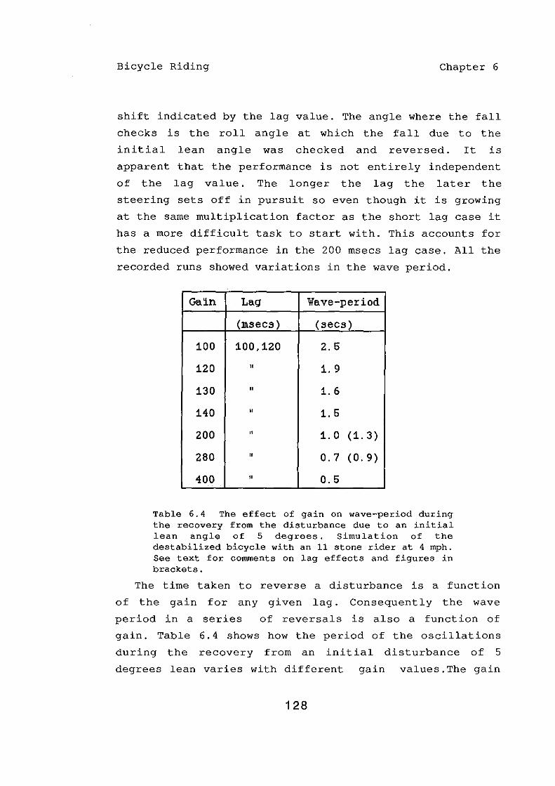
Bicycle Riding Chapter 6
shift indicated by the lag value. The angle where the fall
checks is the roll angle at which the fall due to the
initial lean angle was checked and reversed. It is
apparent that the performance is not entirely independent
of the lag value. The longer the lag the later the
steering sets off in pursuit so even though it is growing
at the same multiplication factor as the short lag case it
has a more difficult task to start with. This accounts for
the reduced performance in the 200 msecs lag case. All the
recorded runs showed variations in the wave period.
Gain Lag Wave-period
(lIIsecs) (secs)
100 100,120 2.5
120 " 1. 9
130 " 1.6
140 " 1.5
200 " 1.0 (1. 3)
280 " 0.7 (0.9)
400 " 0.5
Table 6.4 The effect of gain on wave-period during the recovery from the disturbance due to an initial lean angle of 5 degrees. Simulation of the destabilized bicycle with an 11 stone rider at 4 mph. See text for comments on 1ag effects and figures in brackets.
The time taken to reverse a disturbance is a function
of the gain for any given lag. Consequently the wave
period in a
gain. Table
during the
series of reversals is also a function of
6.4 shows how the period of the oscillations
recovery from an initial disturbance of 5
degrees lean varies with different gain values.The gain
128

Bicycle Riding Chapter 6
is the critical variable controlling the wave period but
once again lag has a small effect. The periods for the
above table were measured by counting the number of waves
on the screen and then noting the time elapsed during
their formation. However for short lags the lower gain
settings produce an almost dead-beat performance and it
was not really possible to do more than make a rough
estimate of where the only wave terminated, thus the
figures given are those for lags of 100 and 120 msecs.
The figures for lags of 60 and 200 agreed where they could
be measured with slight increases in the shorter wave
periods for lag 200 as indicated in brackets.
Summary of Laq/Follow General Characteristics
A repeat of the roll activity in the bar acceleration
channel at some delay is capable of containing
disturbances introduced into the system. The success in
containing these depends on two main factors. First the
gain must be high enough for the bar response to catch and
reverse the roll rate before the angle of lean gets too
high and second the ratio of gain to lag must not get so
high that the system becomes unstable. It has also been
shown that changes in gain lead to substantial changes in
wave period whereas changes in lag have only a marginal
influence. Table 6.S summarizes the various effects of
lag and gain. The heavily outlined boxes show the range of
gain values which give a stable performance for the three
lag values, ranging from unstable due to too little power
at one end to diverging oscillation at the other.
It is evident from the traces in appendix 2, (b) that,
whatever the reasons, the control system in the 12 test
runs is near the lag/gain ratio for the 'just stable'
condition since there is more sign of incipient divergent
instability than dead-beat critical damping. It should not
be expected that the simulator model can make precise
129

Bicycle Riding Chapter 6
quantitative predictions about the detailed performance of
the actual bicycle since a number of the variables
are only approximately defined, particularly the way
the tyre coefficient varies with speed and angle. However
the observed mean wave period of I hertz and lag of 100
msecs with a high degree of oscillation ties in well with
the computer predictions. The 120 msecs lag gives a 0.9
wave period when the gain is such as to put it on the
'just stable' limit. This setting gives plenty of power to
deal with quite large disturbances.
Since the delay between sensing a change of roll and
implementing a change of bar is a sum of various internal
processes it is very unlikely that the value would be
absolutely stable. However this noise alone will not
account for the changes in wave period as we have seen
that the influence of lag on its own is weak. There is a
0.45 correlation between the lag and the roll wave period
for 11 of the 12 runs, indicating that changes in one are
connected with changes in the other. It is obvious that
whenever the wave period changes, there is a transient and
quite strong effect on the local lag value as measured at
the zero-crossing point. A sudden reduction in the wave
period will also shorten one or two lag values at the site
of change. It seems likely therefore that the changes
observed in the lag value are caused by both noise due to
instability and changes in the wave period, with the
latter being the stronger effect.
It seems clear from the behaviour of the simulator so
far is that there is no need for constant change in the
gain when riding the bike in a straight line with low lean
angles. Running as it is around 100 msecs lag with a gain
setting high enough to put it in the stable oscillating
condition it has more than enough power to deal with the
disturbing couple of the weight.
130

Bicycle Riding Chapter 6
Lag Gain Characteristic Disturbance (degs)
2 5 15
200 80 Overdalllped nc nc nc
90 Stable dead-beat 12.8 nc nc
120 Stable Osc. 5.8 16.5 nc
130 just stable 5.7 14.5 nc
140 Unstable Osc. 5.3 13.4 nc
200 Unstable Osc. 4.5 10.7 35.0
120 70 Overdalllped nc nc nc
90 Stable dead-beat 12.0 nc nc
140 Stable Osc. 4.2 11. 0 nc
200 Stable Osc. 3.0 8.0 26
240 just stable 3.0 7.4 23
280 Unstable Osc. 2.8 7.0
60 100 Overdalllped nc nc nc
140 Stable dead-beat 4.2 11. 0 nc
200 Stal:Jle dead-beat. 2.8 7.5 25
280 Stable Osc. 2.6 6.5 20
350 Stable Osc. 2. 5 6. 0 18
170 just stable 2.3 5.5 17
500 Unstable Osc. 2.2 5.5 17
Table 6.5 The effect of gain and lag on stability. Lag in ffisecs, gain in nominal units and figs. in cols 1-3 in degrees. See text for details.
131
Wave period (secs)
-2.5
1.9
1.6
1.5
1.3
-2.6
1.5
1.0
0.9
0.7
-
-1.0
0.6
0.56
0.5
0.4

Bicycle Riding Chapter 6
Control, however, has a problem in establishing just
what that gain setting should be, as differences in speed
affect the balance between the response from the tyre on
the road, which is speed dependent, and the weight couple,
which is not. The tyre response is a value which will also
change considerably between different bicycles and on
different road surfaces and it is not parsimonious to
propose that the rider carries a variety of settings in
memory from which the appropriate value is selected as a
result of sensing the critical variables which affect it.
The Cross-Over model of operator performance of McRuer and
Krendal which resulted from a study of a selection of
compensatory tracking tasks (Summary in Smiley, Reid &
Fraser, 1980) showed that operators adjusted the gain
factor to allow for different system delays, thus
demonstrating that humans are able to alter gain for
control purposes. The simplest solution to the gain
problem would be to try some default value and observe the
response. If this is too low then the gain is turned up
and if too high it is reduced. At the start of a run it is
obvious that the setting will always be high to cope with
the low speed and a large error in initial selection could
be safely corrected by putting a foot back down on the
ground. The result of such a procedure is bound to be
considerable variation in the gain setting during a run
especially since the system prefers to operate with a high
gain putting it near the 'just stable' boundary. Thus,
since wave period is dependent on gain, it can be argued
that at least some of the wave period changes are due to
this cause. Bar movements not connected with the
roll/follow response will also change both period and lag
but whether there is some as yet unidentified additional
input producing this effect must wait until the
characteristic has been analysed to a greater depth.
132

Bicycle Riding
Ti
"
~
Lag
Chapter 6
Ro I I Ue I .
,,-"" Bar "-Roll Reel.
Figure 6.3 Illustrating how the values in the roll velocity channel vary compared with those in the acceleration channel at a sample point shown by the line Ti. The Bar channel is shown as a repeat of the roll acceleration at a delay marked as I Lag T. See text for other details.
Acceleration and Velocity
When the regression analysis was performed on the roll
and bar data in the previous chapter it was assumed that
the roll acceleration information was the only ingredient
being used by the system to modify the bar output.
Control systems however may utilize various forms of the
basic input to achieve different results. Figure 6.3
shows a formalized representation of the roll acceleration
and velocity waves and the bar acceleration wave following
the roll acceleration at a delay labelled LAG. If it is
assumed that the bar value is a repetition of the roll
acceleration then the relevant value associated with the
bar value A is marked at B. At this point the associated
roll velocity value is at C. Because the velocity curve
runs 90 degrees behind the acceleration curve it shows a
maximum value here as opposed to the acceleration value B,
which is zero. Thus the control system could increase its
133
Bicycle Riding Chapter 6
response at low
velocity as well.
acceleration values by adding in the
was at a maximum
Obviously when the acceleration value
the velocity would be making no
contribution. In practice the velocity value could be
obtained from the acceleration by integrating
successive values which is the sort of operation a neural
circuit is well able to perform. In the next section the
effect of using either the acceleration or a combination
of acceleration and velocity on the characteristic will be
explored.
Assume first that the control is only responding to the
acceleration value. When there is a disturbance either
from road irregularities, side winds or a stray
uncoordinated movement by the rider, an acceleration in
roll will result. Since there is a delay in responding,
velocity of roll will accumulate during the interval
between the start of the disturbance and the response
which checks the acceleration. Even when the acceleration
has been removed the velocity will remain and the lean
will continue to ihcrease at a steady angular velocity.
In practice, since the increasing angle of lean will
give an increase in disturbing couple, the acceleration
will start again without any external encouragement and
the process will be repeated with more velocity
accumulating. Figure 6.4 illustrates this sequence on the
computer model running at 4 mph with a lag of 120 msecs
and a gain setting of 240. The bar acceleration is a
repeat of the roll acceleration only.
134

Bicycle Riding
S,"cs BIKE..£ 4
R ( 2)
mph S
(2)
Gain 240 R""
( 7)
<::
Lag 120 S""
(15)
Chapter 6
R" (3)
Figure 6.4 Delay control on roll acceleration only. In this and the following three figures the disturbance is a symmetrical on/off push of 600 msecs rising to a maximum by half-way. The start is marked by an arrow which shows the direction of the effect on the roll acceleration (RI I). The figure at the top of the left axis (4) shows the nominal strength of this push.
From the exact upright position a small disturbing
pulse is introduced. It can be seen that the roll
acceleration (R") is rapidly contained and oscillates
about a mean value that is itself moving slowly left. This
drift is quite clear in the velocity channel, R'. The
velocity that was introduced during the disturbance
remains, so the angle of lean, R, keeps increasing. The
velocity itself increases as well because of the imbalance
between the disturbing and correcting couples with
increasing lean angle.
If the control is now altered to feed both roll
acceleration, R", and velocity, R', into the bar response
the characteristic alters as shown in figure 6.5. Here the
bar is responding to the accumulated velocity value as
well as the acceleration and the former is gradually
reduced to zero in three or four oscillations. However the
135

Bicycle Riding Chapter 6
angle which also accumulated during this operation is not
removed as can be seen by the resulting lean, R. In
general terms the velocity and acceleration introduced by
the disturbance are removed by turning the bicycle into
the lean until the centrifugal force balances the
displaced weight couple.
Secs BIKE..£ 4
R mph S
(2)
Gain 200 R"
Lag 120 S" R'
(3) ( 2)
4
.1
Figure 6.5 (R I , ) arid
reduced to velocity. figure 6.4.
(15)
Delay control on roll acceleration velocity (R'). The gain has been allow for the additional effect of All other values are the same as in
Velocity Contributions in the Recorded Runs
Since the velocity curves (appendix 2, (b)) can be seen
generally to return to the zero line from each wave
excursion they seem to suggest that some velocity
information is being fed back into the bar movement. In
order to test this a multiple regression was run
predicting the bar acceleration values from both roll
acceleration and roll velocity values. Columns 1 and 2 in
table 6.6 show a comparison between the R squared values
for this regression and those from the previous regression
using acceleration data alone. Column 3 shows the
136

Bicycle Riding Chapter 6
significance levels for the multiple regression. All the
acceleration terms remain very highly significant and only
one of the velocity terms falls below p<.OOl to p<.OS.
(Run 28). Again the F numbers for the goodness of fit of
the regression are all well over the critical value for
p<. 001. In every case the R squared value rises, the
actual differences are shown in column 4 with a mean
difference of 3. From this it may be concluded that the
combination of roll acceleration and roll velocity provide
a better prediction of the bar acceleration movement than
the acceleration on its own. In this section of some of
the runs, 32,33 and 34, the combination is accounting for
90% of the bar movement, which when allowance is made for
noise and external disturbances is very high indeed.
This evidence supports the idea that the main influence
on the bar movement is a continuous repeat of the activity
in the roll channel sensed as both changes in acceleration
and changes in velocity. The delay between the two
channels is not absolutely constant but is sufficiently so
to yield very high correlations when a mean value is
used. There are differences between the run sections
analysed here.
correlate at
The R
0.74
squared
with
values for these sections
the original Pearson's
product-moment coefficient values for the whole runs shown
in column 2 of table 6.3. This is an indication that some
runs have more extraneous movement in them than others but
it will be shown shortly that there are also considerable
differences of this sort within quite short sections of
the runs. It will be argued later that this irregularity
is a consequence of one of the essential control features.
Attempts to control using velocity on its own are not
successful because in effect it is the same as increasing
the length of the delay by a quarter of a phase, which
with a basic wave-period of about 1 secs means a minimum
delay of 250 msecs plus any further transmission lag.
137

Bicycle Riding Chapter 6
Section 200-400 Section 200-370 Col Col
accl accllvel 2-1 accl/vel plus angle 7-5 RUN 1 2 3 4 5 6 7 8 9
25 85 87 .001 2 89 .001 89 .001 0 .001 .001 .001
ns 26 74 76 .001 2 76 .001 77 .001 1
.001 .001 .001 ns
27 75 77 .001 2 71 .001 71 .001 0 .001 .001 .001
ns
28 71 73 .001 2 70 .001 71 .001 1 .05 ns .05
ns 29 69 73 .001 4 73 .001 74 .001 1
.001 .001 .001 ns
30 70 74 .001 4 67 .001 67 .001 0 .001 .001 .001
ns
31 82 83 .001 1 83 .001 83 .001 0 .001 .001 .001
ns 32 87 91 .001 4 91 .001 91 .001 0
.001 .001 .001 ns
33 87 90 .001 3 89 .001 89 .001 0
.001 .001 .001 .01-
34 87 89 .001 2 89 .001 90 .001 1 .001 .001 .001
ns
35 78 84 .001 6 84 .001 84 .001 0 .001 .001 .001
ns
36 80 85 .001 5 85 .001 85 .001 0 .001 .001 .001
.01-m.ean 3 0.3
Table 6.6 The R squared terms & significance of the predictors for a series of multiple regressions predicting bar from roll. See text for details.
138

Bicycle Riding Chapter 6
An examination of the upper and lower stability limits
using the same procedure as that applied to the model of
the destabilized Triumph which provided the values for
figure 6.2 using velocity information only shows that the
system is inoperable with such a long delay. There is no
critically stable point since a gain setting which is low
enough to prevent oscillation provides so little power
that the front wheel reaches a critical value before the
fall is contained. If the gain is increased sufficiently
to contain the fall by a reasonable lean angle the system
is so underdamped that it goes out of control before the
second reversal can take place.
Secs
..
J
BIKE..J: 4 R
( 2)
...... ....... ........
mph S
(2)
....
Gain 240 R""
(7)
Lag 120 S""
(15) R"
(3)
Figure 6.6 Delay control on roll velocity (R') only. The gain has been increased slightly to balance out the loss of the acceleration contribution, other values as in the previous three figures.
To provide a comparison with control using acceleration
feedback this condition is illustrated in figure 6.6.
Removing the acceleration contribution reduces the overall
gain so this has been slightly increased to put the first
reversal
quarter
angle on the screen.
phase behind that
The velocity
of the
growth runs a
acceleration,
consequently the gain drives the roll a long way after the
reverse before the velocity value rises far enough to
139
Bicycle Riding Chapter 6
check it. The initial fall is reversed after about 6
degrees but the control is so slow in building up that the
lean has reached 19 degrees to the right and the roll
acceleration has only just reversed. Since there will be
a further delay before the roll velocity reverses there is
no chance of recovery before the lean angle becomes
excessive.
Absolute Angle as an Input Variable
If the control is using only acceleration and velocity,
as described above, the response to a disturbance would be
a stable turn. However if the next disturbance happened
to be on the same side then a further increase in lean
and turn would result and there would be nothing to
prevent excessive angles accumulating after a period of
running. Thus otherwise undirected runs would be expected
to show considerable changes of direction and occasionally
loss of control. In order to keep a constant mean heading
the control must respond to the angle as well. It is
evident from the fact that the subjects kept an
approximately straight course during the runs, even though
they had been instructed not to bother, that the riders
did react to the lean angle or to the rate of turn
which will always accompany lean when under control.
Therefore the next question that arises is whether to go a
step further and include the lean angle R in the bar
response so that the lean angle is also removed, returning
the machine to upright running following a disturbance.
Figure 6.7 shows that the system is well able to
accommodate such a modification. Here the roll angle R
has also been added to the bar response. The increasing
lean, R, acting through the bar rate, forces the velocity,
R', further to the right than in the previous two runs
which in turn brings the lean back gradually to zero in a
series of gentle oscillations and the machine resumes
140

Bicycle Riding Chapter 6
straight upright running. A bicycle controlled in this way
would maintain a straight upright course, gradually
removing any lean angles that accumulated as a result of
external disturbances, which is exactly what happens with
motor-cycles and bicycles at speed.
Secs
.I.
BIKE...c 4 R
( 2)
mph S
(2)
Gain 200 R"
( 7)
Lag 120 s"
(15)
Figure 6.7 Delay control on roll acceleration velocity (R') and absolute roll angle (R). values as in the previous three figures.
R' (3)
(R I , ) I
Other
Evidence Against continuous Angle Control
The appearance of the roll angle traces in the
destabilized runs does not seem consistent with the smooth
removal of lean angle illustrated in the computer
simulation of figure 6.7. Although all the runs maintain
a mean of zero there are constant excursions either side
forming the observed 0.25 hertz wave. In order to test
whether angle was also being used by the delay/follow
system a multiple regression was performed predicting bar
response from acceleration, velocity and angle data. Due
to lack of memory space
the run points had to
in the statistical routine some of
be discarded. The regression is
performed on the first 170 points of the 200 point run
used for the previous regressions, that is points 200 to
370. Column 5 in table 6.6 shows the regression for the
141

Bicycle Riding Chapter 6
two predictors, acceleration and velocity, for the
shorter sections so that it may be compared directly with
column 7 which is the regression for the three predictors,
acceleration, velocity and angle. It will be seen that
removing the last thirty points has revealed some local
differences within the runs but the significance of the
predictors remains above the p<.OOl level except for the
velocity contribution to run 28 which has fallen below the
significance level. The reliability of the R squared
prediction remains well above the p<.OOl level throughout.
Although the reliability of the R squared prediction
remains at the same high level for the three predictors,
column 8 shows that only 4 of the angle contributions are
significant, 3 at p<.Ol and 1 at p<.05. Of these, two at
the p<.Ol level are negative sign which means that to
obtain the overall fit on these runs the angle component
was being subtracted not added. This of course is a bigger
argument against its being a regular contributor than its
being not significant. The other two predictors remain at
a high level of significance with the same sign. Column 9
shows that the change in R squared brought about by adding
the angle term is much less than the change produced by
adding the velocity term shown in column 4 but where it
exists it is always positive.
There is no evidence to support the proposition that
the angle term is used continuously in establishing the
bar movement. However, where the angle term is significant
the correlation improves so it is possible that angle is
being added discontinuously with its sign independent of
the other two continuous contributors. That is there are
irregular short pushes which may work either against the
roll or with it.
142

Bicycle Riding Chapter 6
The Discontinuous Application of Roll Angle
If the underlying control is a delayed repeat of the
roll acceleration and velocity in the bar acceleration on
which some form of angle control is intermittently
superimposed then one would expect the prediction of bar
from roll acceleration and velocity to show similar
discontinuities. The regression analysis gives the
residual values, which are the differences between the
predicted value and the actual value at each data point.
If those which exceed the 95% value (1.96 of the standard
deviation from the mean) are plotted, short runs of
disruption over several adjacent values are revealed. Two
short sections of 50 data points each were selected from
each run, one which included such an area of disruption
and one which did not. The terms 'clear' and 'disrupted'
will be used to distinguish between the two types of run.
Table 6.7 shows the clear sections selected in column 1
and the disrupted sections in column 6. Two clear sections
(Runs 32 and 33) were shorter than 50 to prevent the
inclusion of a disrupted section. The other columns show
the results of regression analyses first with acceleration
and velocity as predictors and then with angle added.
Columns 4 and 9 show the significance level and direction
of the three predictors and columns 5 and 10 show the
change in R squared value which resulted from the addition
of the angle factor.
Throughout all runs the significance of the R squared
term remained well clear of the p<. 001 level. No F
distribution term fell below 100 with a critical value of
11. Some runs showed no increase of R with the addition
of the angle term, some showed a considerable increase and
none showed a reduction. There was slightly more change,
measured by the means, in the disrupted areas but the
distribution of the contributions shows quite a marked
143
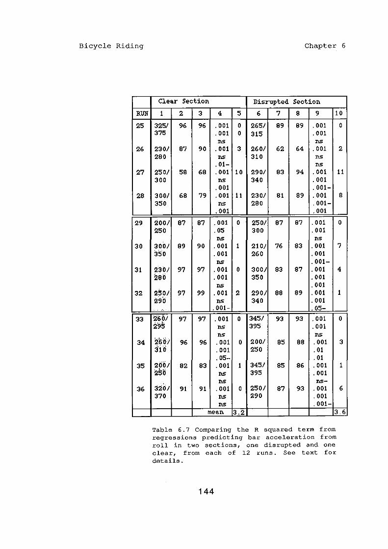
Bicycle Riding
RUN
25
26
27
28
29
30
31
32
33
34
35
36
Chapter 6
Clear Section Disrupted Seotion
1 2 3 4 5 6 7 8 9 10
3251 96 96 .001 0 265} 89 89 .001 0 375 .001 0 315 .001
ns ns 230} 87 90 .001 3 260} 62 64 .001 2 280 ns 310 ns
.01- ns 250} 58 68 .001 10 290} 83 94 .001 11 300 ns 340 .001
.001 .001-300} 68 79 .001 11 230} 81 89 .001 8 350 ns 280 .001-
.001 .001
200} 87 87 .001 0 250} 87 87 .001 0 250 .05 300 .001
ns ns 300} 89 90 .001 1 210} 76 83 .001 7 350 .001 260 .001
ns .001-230} 97 97 .001 0 300} 83 87 .001 4 290 .001 350 .001
ns .001 250} 97 99 .001 2 290} 88 89 .001 1 290 ns 340 .001 .. ,", .001- .05-
2tO} 97 97 .001 0 345} 93 93 .001 0 , I ,~
295 ns 395 .001 ns ns
2'66J 96 96 .001 0 200} 85 88 .001 3 :i1ci .001 250 .01
.05- .01 2dO} 82 83 .001 1 345} 85 86 .001 1 , 0 25 ns 395 .001
. ns ns-320} 91 91 .001 0 250} 87 93 .001 6 370 ns 290 .001
ns .001-mean 3.2 3.6
Table 6.7 Comparing the R squared term from regressions predicting bar acceleration from roll in two sections, one disrupted and one clear f from each of 12 runs. See text for details.
144

Bicycle Riding Chapter 6
difference. Most of the change in the clear runs comes
from two high values in runs 27 and 28. These two runs
also show another difference in that their starting R
values are much lower than the other ten. If these two
runs are excluded then the mean changes become 0.6 for the
clear runs against 2.49 for the disrupted runs which is
consistent with the view that the angle term is having
little effect in the clear sections but is contributing to
the bar acceleration movement in the disrupted sections.
All the acceleration terms remained very highly
signific'nt and positive in sign. Although the velocity
term was highly significant in all but one of the
disrupted runs, five in the clear runs were not
significant, though two of them were in the p<.l bracket.
All remained positive. The contribution of the velocity
term to the regression equation is much smaller than that
of the acceleratibn (means over 20 regressions: velocity
factor 0.030, acceleration fa'ctor 0.834). A possible
explanation of this difference between the clear sections
and the disrupted sections is that there is very little
velocity present in the short clear sections so the
contribution locally falls below significance. An
examination of the traces in appendix 2, (b) is not very
encouraging to this view although it is difficult to make
a clear judgement without some specific criterion.
If it is supposed that the acceleration output from the
semi-circuiar canals is integrated by some neural process
to obtain velocity then such a process is likely to take
some time and may be partly discrete or have some
threshold value below which is does not operate. This
could lead to the more definite appearance of velocity in
the disrupted sections if the disruptions are associated
with more roll movement.
An interesting result is the effect on the significance
levels and signs of the angle predictor. Table 6.8 shows a
145

Bicycle Riding Chapter 6
levels and signs of the angle predictor. Table 6.8 shows a
surnmary:-
Significance Clear Disrupted
NS (p>.l) 7 4
NS (p<. 1 ) 1
S (p<.05) l(neg) l(neg)
S (p<.Ol) 1 (neg) 1
S (p< .. OOl) 3(2 neg) 5(3 neg)
Table 6.8 Showing how well the roll angle predicted the rate of bar change in a clear section and a disrupted section of 12 runs (see text for definitions). Significance of the angle predictor term from the regression is in the left hand column and the number of incidences in either condition for each level is shown in the next two columns.
Since only one significant positive value for angle is
found in the clear runs it is evident that this
information was not making a continuous contribution to
the bar acceleration values. Of the 7 significant
contributions to the disrupted runs four are negative so
it is clear that although there was a contribution from
some source which correlated highly with the amount of
lean angle present, it was not consistently applied in
relation to the existing direction of lean. It should be
borne in mind here that over 50 data points, about 1.5
secs, there is frequently very little change in the lean
angle (~ppendix 2, (b)) so that the contribution to the
regressions for this term is more in the form of a
constant term rather than a variable.
146

Bicycle Riding Chapter 6
Intermittent Control
It seems quite certain from what has been found so far
that the roll acceleration continuously dictates the major
part of the relationship between roll and bar, with a
smaller addition from the roll velocity. Extra movement,
which seems to be correlated with the absolute angle of
lean, is superimposed on this base from time to time. The
disrupted sections analysed in the previous section were
chosen from the excessive regression residuals. To get a
better picture of what these disruptions looked like for a
complete run a routine was written which applied the
multiplication factors for roll acceleration and velocity
found in the regression performed on points 200-400 (Table
6.6, column 2) to the 100-500 sections of the runs shown
in the graphs in appendix 2, (b). Those residuals which
exceeded the 95% threshold were plotted to give the graphs
in appendix 3, (b). A study of these plots shows that the
same general characteristic is to be found for all runs.
There are large sections with residuals below the
threshold and occasional localized sections of 10 to 15
points where the values accelerate to a central peak value
and then fall back again. Sometimes the peaks are isolated
and sometimes they appear close together with the sign
alternating.
The Simulation of Intermittent Peak Inputs
The next thing to discover was the effect on the
characteristic when an intermittent peak input was
superimposed on the continuous activity of the
acceleration/velocity follow/delay system. To simulate
this situation a routine was written which added a given
force to the handle bar by increasing it in equal
increments over a set period and then reducing it to zero
in an equal number of steps. The peak value and period of
147
Bicycle Riding Chapter 6
application could be altered at will. The general
response of the characteristic to these inputs was the
same regardless of these two values.
BIKE..£ 4 mph Secs R S
(3) ( 3)
5 (
7 ..
I
BIKE..£ 4 mph Secs R S
( 3) (3)
iD
1
~ 2 , , c.:. 5 .; ..
" 3 l )
r :"':' , )
f . <"
J. )
I < ..
Gain 200 R"
(25)
Gain 200 R"
(25)
c ::;, <;.:
-~
'-:-
.. '. .~
Lag 120 S"
(60)
Lag 120 S"
(60)
-:':
+-
::> ,
R' (5)
R' (5)
r
Figures 6.8 (a) (upper) & (b) (lower). The effect of pushes of various lengths applied to the simulated bicycle under roll/follow control. The initial disturbance is 2 degs. lean left. The push duration in (a) is 1200 msecs and in (b) is 600 msecs. The arrows show the start of each push.
A push produced a roll in the direction of application.
When the push ceased the underlying roll/bar follow
control removed the acceleration and velocity and left the
148

Bicycle Riding Chapter 6
machine in a stable condition with the accumulated lean
angle remaining as already demonstrated. The amount of
lean change that resulted was a function of the amount of
power applied. That is, a long weak push equated to a
short strong one, however as will now be shown the
characteristic of response did alter with duration of
push.
Figure 6.8 shows the effect on the characteristic of
the simulated bicycle. The values used are the same as
those used in the previous demonstrations. The lag was set
at 120 msecs and the gain at 200 to put the system near
the 'just stable' condition so that there would be plenty
of movement. The machine starts off with a 2 degree lean
to the left. Once the underlying roll/follow control has
removed the disturbance and the bicycle is steady in a
turn to the left a push is applied to force it to the
right. The point at which the push is applied is shown in
the figures by an arrow indicating the direction of
effect on the acceleration trace (R"). Once the lean has
reversed to the right another push is made to force it
back to the left again. The strength of the push (shown
in nominal units to the left of the R axis at the top) is
adjusted with the length of the pulse to give the same
amount of push in each case. Figure 6.8, (a) shows the
effect of a 1200 msecs push of nominal value 5, (b) shows
a 600 msecs push of 10 and (c) a 300 msecs push of 20.
One of the most interesting differences between the
push effects is the behaviour of the velocity channel.
Long pushes force the mean velocity curve away from the
zero for several half-wave periods. One wave is well clear
of the zero, that is it fails to make the zero crossing
and the general displacement of the trace during the large
angle movement is evident to the eye. The 1200 msecs
period is equal to nearly three half-wave periods and the
oscillations in the angle channel are suppressed during
149

Bicycle Riding Chapter 6
the change. As the period of application gets shorter the
displacement of the velocity trace gets less as the main
part of the movement takes place within one half-wave
period (600 msecs is somewhere near the half-wave period
and 300 msecs is well within it). with the shorter pushes
the short wave movement is evident in the angle traces, R
and S, which is also a feature of the real traces in
appendix 2, (a) and appendix 2, (b) .
Secs
:1.0
r.
5
"I
3
:z
I
BIKE..c 4 R
( 3)
-. ') <: , '.., •
,.
~
~
Gain 200 tag 120 R" S" R'
(25) (60) (5)
...... --:;:;,
~ . c:,_ ........
:::~
<. f-<_ -.:;~,
~ c.-:;:--'
< Figures 6.8 (c). The push duration is 300 msecs; all other values as in previous two figures.
Evidence for the Push in the Traces
If it is proposed that part of the control system
consists in imposing short pushes onto the underlying
roll/follow control then it appears from the above that if
the pushes were substantially longer than the half-wave
period of 500 msecs then there would be a large number of
incidents where the velocity wave failed to make the zero
crossing and these would be associated with the pushes.
Although it is difficult to define an exact criterion for
a failure to make a zero crossing since the local
wavelengths show variation, the following table shows an
150

Bicycle Riding Chapter 6
approximation of such occurrences.
Run Detached Location Excessive waves (data pt) Residuals
25 1 330 7 26 0 - 10 27 1 275 3 28 2 280.350 5 29 3 260.320.440 6 30 1 460 15 31 3 310.325.460 4 32 3 200.280.460 7 33 1 425 10 34 4 200.295.370.415 7 35 2 270.380 8 36 7 165.250.310.345 etc. 5
Table 6.9 Showing the number of roll velocity waves which failed to make a zero crossing in the 12 runs and the number of pushes unassociated with roll movement in each run as indicated by the excessive residuals from the regression analysis. Whether the velocity trace crossed the zero line or not was judged by visual inspection and the location of each point is shown in column 2.
The final column shows the number of excessive residual
peaks recorded in each run. There is obviously no reason
for supposing that, if the excessive residual activity is
a place where a directing push is applied, this leads to
the velocity wave failing to cross the zero line. Thus it
can be argued that if pushes are being applied at these
locations they must be shorter than a half-wave. This view
is further endorsed by the fact that none of the excessive
residual runs are longer than 10 points, or 300 msecs.
Attention will now be concentrated on the section of
run 33 from point 350 to 450. Figure 6.9 reproduces the
roll and bar movement graphs from appendix 2, (b) and the
regression residuals from appendix 3, (b) on the same
page to assist in following the argument.
151

Bicycle Riding
Run 33
Angle_ Roll and Bar (dark line)
Yelocit" _ Roll and Bar (dark line)
Acceleration_ Roll and Bar (dark line) \
Regression Residuals greater than t _96 SD_
Data Points
Chapter 6
1
V
111111111111111111111111111111111111111
200 300 400 ::;
Figure 6.9 The first three channels from run 33 in appendix 2, (b) show~ in relation to the excess regression residuals for this run from appendix 3, (b) .
152

Bicycle Riding Chapter 6
The convention applies that movement upwards is to the
left and downwards is to the right. At point 360 the roll
angle (faint line in the top graph) makes a rapid
excursion to the right (down) This is reversed at 390 and
there is a rapid movement to the left which is checked
just after 410 from whence the movement becomes more
gentle. Turning to the regression residuals at the foot of
the page it will be seen that a left bar movement in
excess of that predicted from the roll and velocity
movement is located between 360 and 370.
At point 360 ih the acceleration graph there is a bar
r~sponse (dark line) to the left (up) well in excess of
the roll acceleration. A glance to the earlier part of the
acceleration trace will show that up to this point the bar
peaks more or less match the roll peaks. (The immediately
preceding lower wave which also has an excess peak with an
associated residual peak is ignored at present to keep the
argument simpler). The result of this extra acceleration
in the bar drives the roll velocity response to the right
(graph immediately above) so that it diverges from the bar
velocity. The excess acceleration in the bar is reflected
in the jerk trace by a steeper slope between 355 and 365
(from appendix 2, (b). The jerk trace has been left out of
figure 6.9. ) Despite the extra left bar input the
underlying roll/follow mechanism eventually predominates
as the push declines after its peak value at 365 and the
bar acceleration pursues the roll acceleration to the
right (down).
There is no excess push between 360 and 370 and the
roll/follow movement of the bar succeeds in reversing the
right going roll acceleration just before 370. Even
though the roll has been reversed the bar continues to
accelerate to the right for the delay period (about 100
msecs or a third of one of the marked intervals) thus
153

Bicycle Riding Chapter 6
driving the roll more strongly to the left back towards
the zero line. However at 380 a further small left bar
residual excess appears so this movement is somewhat
inhibited giving the rounded curve in the reverse of the
roll velocity at 380 to 385. At just under 385 a very
strong right bar residual excess appears so that the bar
acceleration which has just begun to pursue the rising
roll acceleration is severely truncated between 385 and
400. This leads to an exaggerated roll velocity peak which
is reflected in the large left roll angle movement back
across the zero line in the upper graph.
By 400 the control, no doubt unwilling to leave the
recovery entirely to the underlying roll/follow system,
puts in two successive excess residual peaks at 405 and
410 to assist in containing the left roll. These have the
effect of holding the bar acceleration on the left side
between 400 and 410 thus driving the roll acceleration to
a very exaggerated right peak at 415 which ties in with
the reduction in the big roll velocity bulge between 390
and 415 and with the termination of the big left roll
movement between the same points in the upper graph.
The above section was chosen for examination because it
was the most exaggerated push in the sample. Equivalent
corresponding movements in the angle, velocity,
acceleration and jerk traces can be seen at the locations
of the other larger excess residuals but are more
difficult to follow as their size diminishes. The exact
shape of the trace which results from such additions
depends on where the push falls in relation to the
existing wave.
Figure 6.10 shows how a small wave adds to a big one
to produce a modification in shape that depends on their
phase relationship. The section of run 33 analysed above
gives good examples of both in-phase and out-of-phase
additions. The downward peak at 350 coincides with the
154

Bicycle Riding Chapter 6
down going acceleration wave and exaggerates its movement
without distorting its shape. The next upward peak does
the same. The small upward push at 385 is in opposition to
the existing wave and cuts its top off with some
distortion. The large peak at 390 is also opposing the
acceleration wave and also distorts its quite badly. Run
27 shows an in-phase addition at point 305 and there are
other examples of both in and out-of-phase distortions
elsewhere, though not always accompanied by excess
residuals.
Figure 6.10 The effect of phase change on the appearance of a wave. The small triangular wave is added to the continuous saw-toothed sine-wave at an increasing phase interval to give the dark wave shape. The bars show the change in wave-length.
Control for Angle of Lean
There should be no surprise at the above findings as,
providing that the main bar response is a delayed copy of
the roll activity then excess values for the residuals
must produce the observed effect. The question is whether
155
Bicycle Riding Chapter 6
the riders are using these pulses to control the machine
Or whether they are accidental inputs. No satisfactory
method of analysis has been discovered by the author for
examining
simulator
lean. The
continuous
has shown
this point conclusively. The runs on the
show that push inputs will produce changes in
regression analysis shows that angle makes no
addition to the bar movement and the simulation
that with only acceleration and velocity
controlling bar acceleration, any angle that accumulates
will remain in the form of a steady turn into the lean.
Since the riders all kept a more or less straight course
during their runs they must have been controlling for
angle in some way Or other and the extra pushes
represented by the excess residual peaks are the most
likely source of this control.
The angle traces show that all the runs have a tendency
for 3 or 4 seconds (100 points equals 3 secs) of a slow
drift of the mean lean angle followed by a fairly sharp
turn back towards the zero, executed within about 1
second. In order to get a clearer picture of how the
excess residuals relate to the movement of the bicycle the
location of the former were printed on the same time base
as the angle of lean curves (light line) from the upper
graphs in appendix 2, (b). These can be found in appendix
3, (c). The arrow direction shows the influence of the
excess push on the existing trace. That is, a residual
shown below the line in the previous graphs, such as that
at point 395 in run 33 (appendix 3, (b)), is shown as an
'up' arrow indicating that extra bar to the right (down)
gives a boost to the left (upwards) roll. Where an excess
residual push is attached to the X=O line it has been
omitted because of difficulty in seeing whether it is the
tail end of a wide pulse or a narrow one. Otherwise all
the recorded pushes are shown and no distinction has been
made between large and small ones. To establish whether
156

Bicycle Riding Chapter 6
the excess residual pushes were in fact associated with
changes in lean angle the following analysis was
performed. The following criteria are taken as dividing
the roll angle response in the region of the pushes into
one of 5 categories.
Case 1. The direction of roll is the same as the
direction of the arrow.
Case 2. The slope changes direction in accordance
with the direction of the arrow.
Case 3. There is no movement either way.
Case 4. The slope is against the direction of the
arrow.
Case 5. The slope changes direction against the
direction of the arrow.
Three 'windows' of 300, 450 and 600 msecs width were
applied successively to each arrow so that the window
exposed the next angle values starting at the arrow
location. Each arrow was given three chances to obtain a
successful rating (case 1 or 2) by successively increasing
the width of the window. As soon as one of the two success
criteria was met the window size was taken as the score
for that arrow. If the arrow failed to meet one of the
successful cases then it was recorded as whichever of the
others was appropriate. The last two cases (4 & 5) were
combined as a single unsuccessful class. The results from
the 93 excessive residual points were as follows:
300 Msecs 66
450 Msecs
600 MSecs
Zero
15
5
o Contra (4 & 5) 7
Although the criteria for judging the slope movement
are somewhat subjective, a very large proportion fall into
the 450/300 mesecs acceptance category. One of the five
600 msec points (run 27 push 3) is right at the peak of an
157

Bicycle Riding Chapter 6
appropriate reversal and only misses a 300 msecs category
because the rule starts the window at the point. At least
one of the contradictory points on closer examination can
be seen to be working in the successful bracket when
combined with the influences of neighbouring pushes. That
is, the effect on the acceleration movement does not
always lead to an observable movement in the angle. (This
was point 7 in run 33, already dealt with in detail
above. )
The above results suggest that the excess residual
pushes do lead to changes in the roll angle. It can also
be seen, especially in the first five runs, that the rapid
changes in angle already noted frequently have associated
residual arrows in appropriate locations. However it is
also true that there are some large angle changes with no
associated residual peaks. Run 25, point 240 provides one
example, run 27 point 200 another. Presumably there could
be a large peak just below the 1.96 threshold which got
its power from time of application rather than amplitude
and is therefore masked by the noise. The failure of an
arrow to appear on the first reversal of a long rapid
roll mo~ement such as at run 26 (265), rUn 27
(215) (360) (390) & run 29 (390) is not surprising as the
computer simulation shows that the roll/follow response to
a large externally imposed movement reduces the rate of
roll almost as quickly as the initiating movement. (figure
6.6 (a) Reversal at 2.5-3.0 secs). The pushes which follow
the initial reversal in the examples quoted would be
consistent with a rider putting in a push to counter the
shallow oscillating drift that follows the initial strong
reversal and force the bicycle back towards the upright.
Although it seems clear that the pushes identified by
the excess residual peaks are causing the bicycle to
change its roll angle it not so easy to establish what
feature might be triggering these inputs. The absolute
158
Bicycle Riding Chapter 6
angle values for roll are unreliable as they are the
result of integrating the recorded velocities and the
constant term has been established only approximately.
The bar trace, which records actual angle not velocity,
has been used as a guide for 'zeroing' the angle data but
the exact distance of the various excursions from the zero
line are only approximate. It should also be borne in
mind that the angles involved here are small, less than 2
degrees. There are a number of examples of quite sharp
turns from apparently upright running (run 27,{320), run
33,{370)), but in general there are no sudden turns away
from the zero line when the lean angle is already
substantial. That is, any drift in lean is always curbed
not exaggerated. Thus the overall impression is that
somehow the control detects lean angle rather
approximately and, when this exceeds some threshold value,
pushes are used to bring the angle back towards the zero.
In the last three runs several alternate left/right
pushes have been introduced when the bicycle is running
upright, which make no overall change to the angle but
produce a comparatively large local wiggle. Feedback
control systems depend upon the changes in the primary
signal for their operation. When the signal gets too weak
it becomes swamped by noise and the control 'dithers'
about the zero waiting for something definite to appear.
Hunting to and fro either side of zero is one way of
improving the signal to noise ratio. Initially it was
supposed that the rider might be injecting short ballistic
pulses, timed to coincide with the zero crossings of the
roll acceleration, to give an increased response. However
a' more parsimonious explanation is that riders increase
the gain value to approach, or even temporarily exceed,
the 'just stable'
oscillations in
condition which results in large
the acceleration channel without
associated changes in the mean roll angle. When, however,
159

Bicycle Riding Chapter 6
the bicycle is balanced near the upright there is little
actuating signal so the gain has nothing to mUltiply and a
high value will not produce a rapid change. It is
therefore possible that the left/right pushes observed
here serve the purpose of disturbing the upright balanced
position in order to improve the actuating signal.
Since the blindfolded riders had no direct information
about absolute angle they could only have recovered such
information either by some sort of neural integration of
the rolling and yawing acceleration or from sensory
changes at the contact points with the bike due to the
centrifugal forces during the turns. With the very small
angles involved the latter changes would be very small
indeed and the integrations would suffer from the same
sort of inaccuracy due to lack of the constant term as is
found in the data conversion. Both of these could account
for the lack of any clear regularity in the application of
pushes as r~vealed by the excess regression residuals.
Combined Intermittent and Continuous Control
A high correlation was found between the roll and bar
activity throughout all the runs, rising to a
places where the roll acceleration and velocity
accounted for over 95% of the movement in
acceleration (col.2, table 6.7) and was above
peak in
activity
the bar
SO% for
every total run (col. 2, table 5,3). Since the only
movement to the handle bar is through the rider's arm
movements it can be concluded that the basic control
system used by the riders applied the rates of angle
acceleration and velocity sensed in roll as rates of angle
acceleration to the handle bar after a delay that varied
about a mean of approximately 100 mesecs. The failure of
the angle term to maintain significance and constant sign
in a multiple regression over several seconds of run time
(col.S, table 6.6) indicated that angle was not
160

Bicycle Riding
continuously applied in
simulation showed that,
Chapter 6
the same way. A computer
with only acceleration and
velocity controlling the bar, the control failed to remove
angles that accumulated, thus a bicycle using such a
system would end up in a turn which would get tighter and
tighter depending on which way random disturbances
affected it. Th"e fact that the riders did remove turns
during the runs showed that angle must have been fed back
into the control in some form. When the points where
excess bar angle acceleration over that predicted by the
roll angle acceleration and velocity were plotted on the
same time base as the angle movement they were frequently
(87%) associated with an appropriate roll movement within
a half-wave length (mean 0.5 secs), but there were a
number of containing movements which did not have
accompanying excess residuals associated with them.
Simulated runs showed that pushes imposed over periods
greater than a half-wave length led to distortions in the
velocity curves which were not observed in the run graphs.
It was also noted that the maximum period for the excess
residual peaks was 300 msecs.
Overall it is considered that the evidence suggests the
riders were using a continuous delayed feedback control
which removed acceleration and velocity in a series of
'just stable' oscillations. As ang le accumulated some
threshold was exceeded and a push or series of pushes were
added to the continuous control to oppose the lean. The
small lean angles involved and the lack of direct
information about absolute angle led to a rather noisy
operation of the intermittent part of the system but the
general trend was a slow increase of lean during a series
of short wave oscillations and a short sharp change of
angle back towards the zero, which was then either checked
again with further pushes or allowed to settle down into
another slow change before the threshold for action was
161
Bicycle Riding Chapter 6
again exceeded. The intermittent pushes were of a
ballistic nature, showing an exponential rise to a peak
and a similar decay. These pushes did not replace the
underlying movement but were added to it to produce a
composite wave form which means they must have been angle
independent, implying a muscle tension independent of
length. They were not timed in relation to the underlying
movement as they sometimes enhanced a wave and sometimes
inhibited it.
Variations in Lag and Gain
Change in lag, wave period and area was a feature of
all the runs. It is fairly certain that the phase lag and
gain would show small random changes about some mean even
if the control had no reason for altering them since
they are the consequence of neural operations which are
unlikely to be absolutely stable. Change in lag on its
own merely alters the potential stability of the system
and cannot be seen as an effective controlling
variable, and once the lag is fixed then the gain is also
fixed to give the best response without going into the
unstable condition. Thus it is argued that lag and gain
are reasonably stable values which remain fixed so that
the bar/roll follow control can operate effectively. It
can easily be seen that a push superimposed on an
otherwise perfectly regular bar/roll follow wave form will
cause large local disturbances to both the lag and
wave-period. Over the l2 runs there was an average of one
excess regression residual every 1.5 secs (12 runs of 400
points, ie 12 secs, 93 pushes) so it is evident that there
would be a good deal of disruption from this source and
since the pushes are not driven by the roll change the
initial movement would not be highly correlated with
that in the roll channel. As the roll follow responds to
the disruption the phase error is removed and the two wave
162

Bicycle Riding Chapter 6
periods correlate more closely.
Thus it can be seen that it is a consequence of a
control where uncoordinated short pushes are superimposed
on continuous wave/follow activity that there will be
disruptions to the lag and wave periods which are
partly correlated between the roll and bar channels.
only
The
wave areas on the other hand are a reflection of the power
applied and will correlate more closely when the system is
maintaining a controlled path near to the upright. A
larger than normal bar push suddenly introduced does not
lead automatically to a large area for that wave as can be
clearly seen in run 33 (figure 6.9) around point 400,
since the extension of wavelength allows the amount of
power applied to balance. Referring back to table 5.4 in
chapter 5, it was noted that when the overall correlation
was high there was a more stable wave-period. This ties in
with what has been learned about the disruptive effect of
wavelength change on correlations and the conclusion is
that the wavelength disruption comes from uncorrelated
pushes added to the relatively stable underlying bar/roll
follow control, rather than changes in the lag or gain per
se.
Imitating Full Control on the Simulation
Figure 6.11 shows the simulated bicycle running under
fully automatic control with the speed and response values
trimmed to approximate those of the real runs. The bar
acceleration is a repeat of the roll acceleration and
velocity channels delayed 120 msecs. The gain has been set
at 220 to put the system near to the 'just stable'
condition to mimic the movement found in the real traces.
The intermittent rule applies a push of nominal value 16
applied over 300 msecs whenever the angle exceeds a
threshold of 1.6 degrees. To avoid applying a second push
before the first has had time to produce a change in the
163

Bicycle Riding Chapter 6
lean angle, further pushes are locked out for one
half-wave period. The points at which the intermittent
control applies a push are shown by an arrow which relates
to the acceleration traces using the same convention as
before. The arrow points in the direction in which the
angle is driven. Figure 6.12 shows the first part of the
same run in a horizontal format similar to the one used
for the real run records so a comparison between the
general characteristics can be made more easily.
Secs
7
6
5
'" 3
2
~
Bike...£ 3 mph Gai n 220 La!) 120
R S R" S" (2) (5) (45) ( 142)
1.6-( )
\ .-(" ...
':-r'
~ ...
'-..J.. ) ...
Figure 6.11 Simulated automatic control. Basic control is repeat of roll acceleration & velocity at a delay of 120 msecs with the gain set to give a Ijust stable' response. When lean angle (R) exceeds 1.6 degs a 300 rnsecs push is added to the basic control to bring the lean back towards the vertical. Each push is shown by an arrow.
R' (5)
It can be seen that the intermittent threshold rule,
superimposed on the continuous roll/copy/delay control,
164

Bicycle Riding Chapter 6
produces a trace that is very similar to those of the
actual runs. The local distortions to the roll
acceleration trace seen at 3.5, 5 and 7 secs, caused by
the addition of the triangular short push to the
underlying wave, may be compared with the distortions
shown in figure 6.10 and similar shapes in the run traces.
Bike.J: 3 mph Gain 220 Lag 120
.,....-7"'::., .. Angle
Velocity
Accln
1 2 3 4 5 sees
Figure 6.12 The initial 5 secs. of the run shown at 6.11 turned through 90 degrees to assist comparison with the record from the experimental bicycle under the same running conditions.
Nested Control Loops
Smiley et al. (1980) studied how the control technique
of naive car drivers altered with learning. When subjects
first started the task they tended to remove lateral
displacement errors by altering heading until the
displacement began to decrease and consequently
over-controlled. Since they also made corrections to
heading errors, independent of displacement errors, the
solution to the first problem led to a contra-response
from the second. In effect the two loops worked against
each other instead of in unison. As they gained
experience the subjects altered their technique so that
165
Bicycle Riding Chapter 6
the two control loops were nested. A displacement error
was corrected by demanding an appropriate angle change in
the heading loop which continued to operate about this new
value until the displacement had reduced, at which point
the heading demand was returned to the original zero.
In the proposed control for the destabilized bicycle no
such nesting takes place. The underlying roll angle
acceleration and velocity loop continues to operate
autonomously. The push demand temporarily overpowers the
continuous control and imposes a roll errOr upon it. In
automatically removing the roll error the bicycle is
turned into this lean error which is the solution required
by the push. A similar performance is seen in bipedal
balance when runners sprint from starting blocks. The
initial instability is solved by accelerating the centre
of mass as fast as possible in the direction of lean. In
the bicycle the acceleration is provided by the turn
rather than the linear acceleration of the sprinter, but
it has the same characteristic in that it solves the
toppling problem by altering the acceleration of the
support point relative to the centre of mass.
Summary.
This chapter has explored the control technique used by
the subjects riding the destabilized bicycle in a straight
line, blindfold at very low speeds. In this condition a
normal bicycle has very little natural stability and the
experimental bicycle had none. The riders achieved basic
balance by repeating the roll acceleration and velocity as
steering angle accelerations. This allows absolute angle
to accumulate. When some lean/turn threshold was exceeded
the bicycle was forced back towards the upright with a
short pulse lasting less than half a wave period. The
next chapter considers how this control system might be
applied to the conditions found in normal bicycle riding
166

Bicycle Riding Chapter 6
where the contribution of autostability becomes
significant.
167

Bicycle Riding Chapter 7
7. CONTROL OF THE AUTOS TABLE BICYCLE
Normal Control
The previous two chapters examined in detail the
control used for riding a bicycle with all the
autostability removed. This chapter will deal with the
application of what has been learned to the problem of
controlling a normal bicycle. Three qualifications affect
the records taken from the normal bicycle. First the
limited length of the recording wire prevented any fast
runs. Second the records of bar movement contain
contributions from two sources, the riders' arm movements
and the autostability responses of the bicycle, and there
is no way of discriminating between these. Also, because
lateral body movements lead to autostability responses,
some of the controlling movements may come from this
source without there being any indication of this in the
records. Third, all the normal runs were done on the
Triumph bicycle before its conversion, consequently these
records differ from the ones already presented not only in
the presence of autostability but also in the extra weight
of the conversion. This, together with the remote steering
linkage, slightly altered the inertia and friction in the
steering assembly.
Low Speed Control with Autostability
A short summary of the autostability effects will be
given as a preparation for the discussion of normal
control. Due to the front-fork design three couples act
continuously on the front wheel. Whenever the frame is
rolling there is a precessing force trying to turn the
front wheel in the direction of the roll. Any increase in
the angle between the front wheel and the direction of its
168

Bicycle Riding Chapter 7
local travel will produce a restraining couple, due to the
castor effect, which inhibits the movement. Whenever there
is an angle of lean the castor effect also gives a couple
trying to turn the wheel in the direction of lean. The
higher the speed the stronger the first two effects. The
greater the angle of lean the smaller the last two become,
because the geometry reduces the effective trail distance,
but this effect is not of major importance at normal
riding angles. These effects can only apply if the front
wheel assembly is quite free to turn under the influence
of the couples.
Autostability depends for its effect on speed. When the
speed falls below some limit there is insufficient
response
rider.
to prevent
The next
a fall without assistance from the
section discusses the differences
between ten runs on the normal bicycle with those already
discussed for the destabilized machine. The same subjects
provided five runs each and the conditions were exactly
the same in every respect as the destabilized runs except
that the bicycle was the Triumph 20 before conversion.
The traces of these runs are not presented but to a
casual inspection they are indistinguishable from the
destabilized runs reproduced at appendices 2, (b) and (c).
In order to compare the two sets of runs the values of the
matched waves, the extraction of which was described in
detail in the previous chapters, will be used.
Table 7.1, columns 1 and 2, shows a comparison between
nine characteristics of the two types of run. Column 3
shows the significance of a t-test between the two sets of
means. The justification for using the t-test is based on
the following argument. It is evident that during a run
the value of some variable such as 1ag or wave-length is
very definitely influenced by preceding values and
therefore violates the assumption of sampling independence
required for the t-test. However, if it is assumed that
169

Bicycle Riding Chapter 7
the mean value for lag delay or wave-length or wave area
during a single run is a characteristic of the system
representing the combination of the bicycle and the rider
then it is reasonable to argue that there exists a
population of such mean scores which will be normally
distributed about some mean value over a large number of
similar runs. When some single value is changed, in this
case the change from the normal to the destabilized
bicycle, then this distribution either changes or remains
the same. Although the values for several successive runs
are still not truly random samples from this population
the t-test used has some validity in indicating whether
there are differences or not.
Variables Col. Norm. Destab Sig.
CCF roli/bar full run
Lag. Mean counted vals
Roll half-wave period
Bar half-wave period
Roll wave area
Bar wave area
Stand.dev. bar/roll
Corrln. roll/bar waves
Corrln. roll/bar areas
1 0.86
2 3.6
3 13
4 10
5 88
6 44
7 0.36
8 0.32
9 0.64
0.85 ns
3.7 ns
12 ns
11 ns
115 .01
103 .001
0.67 .001
0.56 ns
0.77 .001
Table 7.1 Comparison between the normal and destabilized runs for nine variables. Lags and wave-periods are in data-point intervals (30 msecs) and areas in nominal units. Values in rows 1 and 7- 8 are corrected to 2 places decimals, those in row 2 to 1 place decimals and in rows 3-6 to the nearest whole number. See text for details of t-test to which the last column refers.
Since the samples were not of the same size and
nothing was known of their variances a t-test of two
170
Bicycle Riding Chapter 7
unrelated samples was used, (MICROTAB twosample). As will
be seen the correlations between the roll and bar angular
accelerations for the full run show no difference.
Although there were some differences between the two
individuals in the distribution of their lag values during
a run it can be seen that the combined mean values
over a run for either bicycle remain the same. Also the
mean half-wave period for the matched waves show no
significant differences. However the areas of the matched
waves in the destabilized system were significantly larger
than those for the normal bicycle, with a greater
difference in the bar than the roll.
The above results seem consistent with a combination of
autocontrol and human roll/follow control at low speed.
The autostability, which works almost instantly compared
with the rider's control action, reduces the roll angle
movements arising from both external disturbances
and the overcontrol due to the slower corrections of the
delayed human responses, but the speed is too slow for all
the movement to be removed. The wave period, which is a
consequence of the lag/gain ratio and the dynamic
properties of the system, remains the same in either case
but the areas which represent the power applied are less
than the roll areas because the automatic control is
limiting the roll departures earlier and therefore less
bar is needed tb contain them. The bar area is also
proportionally less in the normal bicycle output. Row 6
shows a cornparisbn between ratio of bar angle standard
deviations from the mean divided by roll angle standard
deviations. This is a measure of how much bar movement is
needed to contain the roll movement and confirms that the
autostable control requires less. At least two factors can
be identified which would promote such a difference. First
the greater the absolute lean angle the greater the
disturbing couple due to weight displacement so more bar
171

Bicycle Riding Chapter 7
is needed to check a larger angle of lean, and, since the
autostability is checking the roll more quickly than
before, the angles will be smaller. However the angles of
lean in all cases were very small (see table 5.1) and it
is hard to see how a difference of 1 degree could cause
such a difference since the sine value hardly changes in
this regime. A second possibility is that the greater
inertia and less positive action in the modified front
fork design of the destabilized bicycle leads to greater
overcontrolling. The castor effect in the normal bicycle,
which works against all movements that try to push the
front wheel out of alignment with the direction of travel,
would also tend to damp out any overcontrolling due to
steering assembly inertia.
As expected row 7 shows that the correlations between
the roll and bar half-wave period are not significantly
different, although those of the normal bicycle are
slightly les~ correlat~d. However the areas do show a
difference although it is not clear why this is so. It
appears that for some reason when riding the normal
bicycle, although the subjects made proportionally less
bar movement per roll movement, more of this movement was
unrelated to associated movements in the roll. There is
the possibility that this was a learning effect since the
normal runs were done near the beginning of the
experimental period whereas the destabilized runs were
done after both riders had acquired considerable
experience of slow blindfold riding. That is, the extra
uncorr~lated bar movements could be noise due either to
unstable gain values or accidental or exploratory pushes.
In summary the comparison between runs on a normal
bicycle and runs on the destabilized machine at very low
speed shows few differences, which is consistent with the
idea that the autostability of the front forks is only
providing a marginal assistance to the human
172
Bicycle Riding Chapter 7
roll-follow-at-a-delay control explored in the previous
two chapters.
Controlling the Normal Bicycle at Speed
The next question to be discussed is what control
movements the rider uses to direct an unmodified bicycle
at normal riding speeds. It has already been mentioned
that recordings of rider activity with a normal bicycle
are contaminated by the autocontrol. However with the
assistance of the simulation and some general observations
at fast riding speeds a fairly clear picture of the
necessary control system can be constructed.
General Observations on Fast Riding
The following experimental runs were made to obtain the
general response of a normal bicycle to some simple
control inputs at a speed where the autostability control
had enough power to remove any accidental roll errors. The
rider was a male weighing 178 Ibs in good current practice
riding a Carlton ten-speed sports tourer in good
condition.
a normal
Five runs were made
road surface
in each configuration on
down a hill whiCh was
sufficiently steep to maintain the speed without
pedalling. The speed did not need to be known accurately
but at the start of the each run the pedalling speed was
approximately 2 to 3 half-cycles of the pedals per second
in top gear (14/52 pedal/wheel ratio. 26 inch wheel).
This equated to between 17 and 23 mph at which speed there
was a high degree of autostability. Throughout the test
runs the rider made every effort to prevent any movement
between body and bicycle.
1. Inherent stability. The rider aimed to negotiate a
200 yard section of road without touching the handle bars
and without moving his body. The bicycle was extremely
stable with quite high forces in the steering due to the
173

Bicycle Riding Chapter 7
autostability factors. On four out of the five runs the
bicycle ran straight and upright down the middle of the
road. On one run a single adjustment was made to heading.
2. Response to a disturbance. Once established in the
hands-off running configuration described in 1. above, the
rider pushed forward briefly with one finger on one handle
bar. The immediate response was a sharp lean towards the
side of the push. This was followed by a very rapid return
to upright running with one or two decaying oscillations
in roll either side of the vertical as the effect of the
disturbance damped out. A small change in direction
accompanied the correction.
3. Response to a steady push. From the hands-off
running configuration the rider applied a gentle push with
one finger to the end of one handle bar. The tip of the
finger was used so that only a push could be applied. The
push was held as constant as could be judged. The response
to this input was a rapid lean in the direction of the
push but this time there was no recovery. If the push was
applied rapidly there were a number of damping
oscillations about some mean angle of lean in the
direction of push; If the push was applied slowly the
angle gradually increased without oscillations. In both
cases the lean stabilized at an angle that depended on
the strength of the push and the bike went into a steady
turn in the direction of lean. Although the push was
maintained the handle bar reversed rapidly in the
direction of the lean under the autostability forces
during the start of the lean and during the turn the front
wheel was turned slightly in the direction of lean/turn.
4. Recovery from a turn. Once established in the turn
described in 3. above the rider rapidly removed the
pushing hand so that both hands were well clear of the
handle bar. The response was a rapid roll back to the
upright. This continued over the vertical so that there
174

Bicycle Riding Chapter 7
was a fairly large excursion of lean to the opposite side.
Depending on the steepness of the original turn there were
two or three damping oscillations in roll either side of
the upright and the bicycle returned to straight steady
running.
5. Modified recovery. In this configuration the push in
the turn was removed smoothly and gradually rather than
suddenly. The response was a smooth gradual recovery to
upright running.
It was not possible to say for certain that there were
no associated body movements modifying the autostability
forces during these manoeuvres but the rider made every
effort to ensure that none was made and if there were any
unconscious movements they must have been very small. The
effects observed were exactly what would be expected from
an understanding of the autostability design of the
bicycle. Left to its own devices the autostability
resisted any tendency of the front wheel to leave the dead
ahead position. Any roll was removed by the gyroscopic
effect. Any lean was removed by the castor effect.
When the steering was displaced during upright
running with a short push a turn resulted in the direction
of the steering displacement, that is towards the side
opposite to the push. This turn led to a roll 'out of the
turn', that is towards the side of the push. This roll
caused the front wheel gyroscopic effect to produce a
precessing movement of the bar in the direction of fall.
This movement of the steering started a turn in the
opposite direction and thus balanced the fall.
When the bicycle was leaning over in the turn the
weight of the rider and the machine acted via the castor
effect to produce a couple with the trail distance,
turning the wheel further in the direction of lean. This
gave a greater centrifugal rolling effect than the
displaced weight couple and the bicycle was rolled back
175

Bicycle Riding Chapter 7
towards the upright. These effects worked in unison to
remove any lean angle in a series of oscillations either
side of the upright.
When the autostability was modified by holding a steady
push to one side (out of the turn) the extra angle due to
the castor effect was opposed and the bicycle stabilized
in a turn. The gyroscopic force at this speed overpowered
the steering push and the resulting movement against the
push was an addition of the two couples. It should be
remembered however that at some steering/roll angle
combination depending on the design of the bicyle the
effective trail distance is reduced to zero and actually
becomes negative if the angle of lean increases any
further. (For example with the Carlton Corsair a steering
angle of 10 degs maintains a positive trail distance to
over 35 degrees of lean but an increase to 15 degs
steering reverses the trail effect at about 25 degs lean.)
Thus at very steep angles of lean the rider must modify
his technique in this respect. At some point the machine
becomes neutrally stable in roll and will keep turning
without any bar pressure. Beyond this angle it will become
increasingly unstable and will need into-the-turn pressure
to prevent its going out of control. This almost certainly
accounts for the 'uneasy feeling' encountered in fast
steep turns typically when negotiating a roundabout.
The above effects could only be seen in this clear form
when the speed was high. At low speed the autostability
forces were low compared with the disturbing effect of the
couple caused by the displacement of the centre of mass to
one side of the support point so that greater angles of
lean and rates of roll velocity were reached during the
corrections. Below some low speed the autostability forces
on their own were not enough to contain the disturbing
couple and had to be supplemented by movements from the
rider. It was noted that these movements tended to
176
Bicycle Riding Chapter 7
include extra roll induced by upper body movements either
as well as or instead of additional arm movements. The
latter could not be subjectively experienced. The fact
that they must have existed was deduced from the fact that
when the hands were removed from the bar at low speed
control was lost.
The Effect of I?ushes on Control
It can be seen that the basic method of controlling the
normal bike for changes in direction is similar to that
seen in the destabilized bicycle. That is a push is added
to the continuous movement of the autostability control.
There is, however, an essential difference between the two
underlying systems. The destabilized control responded to
roll velocity and acceleration whereas the autostability
of the front forks in the normal bicycle will respond to
lean angle as well. When the speed is high, angle as
well as roll rate is removed and the bicycle will return
to upright running under autocontrol. A single on/off push
causes the destabilized system to take up a turn whereas
it merely causes a temporary disturbance in the normal
bike which returns to upright running as soon as the push
is removed. In order to keep the bicycle turning in the
latter case the push has to be maintained.
This difference is illustrated on the simulated model.
Figure 7.1 shows the effect of a single on/off push on
each in turn. The time of application of the disturbing
push is the same in both cases but the force has been
adjusted to give exactly the same initial excursion of the
handle bar acceleration (S' '). Because the castor effect
produces a strong damping effect on any steering movement
out of true the force needed to produce a similar effect
on the bar is higher by a factor of 5. In the upper
diagram the simulation responds in the same way as the
bicycle in the high speed tests in that the initial
177

Bicycle Riding Chapter 7
disturbance is damped out after two decreasing
oscillations and upright running is rapidly resumed.
Secs
a
2
J.
Secs
BIKE..£ R
8 mph
( 2)
BIKE..£ 8 R
( 2)
S ( 2)
mph S
( 2)
(
Norma 1 bicy c le R·· S··
(50) (70)
Gain 220 R"
(50)
Lag 10 s"
(70)
R' (5)
R' (5)
Figure 7.1 The effect of a single on/off push on the autocontrol. (upper graph) and destabilized system (lower graph). The push is applied over the same time interval with the strength trimmed to give the same initial response from the steering acceleration (S") .
In the lower diagram the roll acceleration (R") is
damped out with the trace showing a mean of zero. The
velocity (R') is initially displaced to the left by the
push but returns to a mean of zero after about 3 seconds.
178

Bicycle Riding Chapter 7
The angle
and the
incurred during this operation is not removed
destabilized bicycle continues to lean and
therefore turn in the direction of the disturbance (R).
The scale in the roll channel has been left large
deliberately so that a direct comparison may be made
between the two figures. The gain and lag in the
destabilized control has been chosen to give a lightly
damped converging oscillation.
Secs
3
J.
8IKE.J:
388
R (5)
12 mph S
(2)
Normal bicllcle R"
(50)
~ . ..... -
s" (75)
R' (10)
Figure 7.2 Simulation of push control of the autostable bicycle at 12 mph. A single 'on' push turning the bar to the right (right peak in channel S'I at 0.3 secs) gives a smooth roll to the left. The autostability forces immediately respond and check the lean at 7.5 degrees giving a steady turn left until the push is removed (left peak in S" at 2.25 secs) when it returns to upright running without further attention.
179

Bicycle Riding Chapter 7
Controlling the Normal Bicycle in a Turn
It was seen in the high speed tests that a push held on
the bar led to a balanced turn in the direction of push at
a rate that depended on the strength of the push. It was
also seen that gently removing the push once in the turn
led to a smooth recovery to the upright. Figure 7.2 shows
this operation simulated on the model at 12 mph. The
push to the right causes an excursion of the bar in that
direction (S) . The autostability forces rapidly oppose this
and under the combined effect the bar moves to the left to
follow and contain the fall by 7.5 degs. The result is a
steady lean and therefore turn to the left. When the push
force is removed at just over 2 secs (note the sudden
left excursion in the steering acceleration channel S")
the unrestrained castor effect moves the bar further left
causing the centrifugal couple to dominate the falling
couple and the bicycle returns to the upright with one
gentle oscillation. Thus the technique for turning a
bicycle at a speed where the autostability is high is to
apply a gentle push in the desired direction of turn,
maintain the push until it is time to recover and then
remove it upon which the bicycle automatically resumes
upright running.
The faster the speed, and therefore the higher the
autostability forces,
strength of push.
the smoother the response to a given
When the speed falls and the
autostability forces begin to reduce, the push must also
be reduced to keep the control smooth. Steep turns at low
speeds are therefore likely to be more oscillatory.
Unfortunately no systematic recordings were made of
manoeuvres but some rather casual recordings were made
early on of the entry to and recovery from a turn with the
normal bicycle at about 7 mph. Unfortunately two of the
subjects were unable to carry out this manoeuvre without
going out of control and their productions are of little
180
Bicycle Riding Chapter 7
use except as an interesting example of overcontrolling.
However one subject produced a good trace of a smooth
entry to and recovery from a turn and this is shown in
figure 7.3.
Run No. 10 Roll and Bar (dark lines)
ANGLE
VELOCITY
ACCLN
I I I I I I I I I I I I I I I I I I
data points 100
I I I
200
I I I I I I I I
3
Figure 7.3 Showing the angle, velocity & acceleration for roll and bar (darker lines) for a 360 degree tUrn (Run 10) on the unmodified bicycle with a sighted rider. See text for details.
181

Bicycle Riding Chapter 7
Single Recording of a Successful Turn
This run was made on the normal Triumph 20 bicycle
before modification. The recording was made at an early
stage of the experiments when the recorder was using four
channels instead of two which gives an interval of 56
msecs between recorded points. The rider was the same
subject who produced the high speed observations and for
this run he was not blindfolded. The instructions for the
run were as follows. The rider accelerated to a
comfortable riding speed on a course which took him back
along the wire and across the front of the recording
station. The recorder was started as soon as run speed was
achieved. At some point approximately opposite the
recording station the experimenter called 'now' and the
subject initiated a turn to the right as quickly and as
steeply as possible consistent with smooth control. The
turn was continued for 360 degrees holding as steady an
angle of lean as possible at which point a smooth
recovery was made. The run was terminated once straight
running had been resumed. The actual mean angles during the
turn were 9 degrees of lean and 5 degrees of bar. The
radius of the turn was measured as approximately 15 ft so
the speed can be calculated from the equation:-
Force = Mass x Speed A 2 / Radius
where the force is that needed to produce a couple to
balance the weight couple at 9 degrees lean with a weight
of 200 lbs and a lever arm of 3 feet. This gives a speed
of 6 mph. This also cross checks with the time for the
turn recovered from the graph of the run. A 15 ft radius
turn has a diameter of 94 ft which takes 11 secs at 6 mph.
There are 200 points of 56 msecs each between the
initiating spike and the recovery, ie 11.2 secs.
It is not possible to discriminate between arm induced
182

Bicycle Riding Chapter 7
bar movements and secondary effects due to body lean in
the traces from the normal bicycle. Whichever method is
used, and there is a likelihood that a combination of both
methods is the normal technique, the only way a rider can
initiate a large roll rate is by moving the bar to give a
turn in the opposite direction to the desired roll. Figure
7.3 clearly shows this initiating movement of the bar at
the start of the turn in all three graphs and the
corresponding rapid increase in roll angle. For about 80
points after the initiation there is some 1 hertz
oscillation which damps out. Between points 160 and 210
the record shows very little movement in the rate traces
which is due to the inability of the recording system to
capture the reduced movement when the bicycle is under
autocontrol alone. The extra filtering in the jerk trace
removes all the bar movement and most of the roll between
the initiating spike and the recovery so this channel was
not included in the figure. After the recovery there is a
resumption of the 1 hertz oscillation. This record shows
that the rider was able to hold a steady push on the bar
between point 160 and 210 which just balanced out the
castor effect and left the bicycle turning steadily under
the gyroscopic effect.
Table 7.2 shows the statistics for this run. Because
of the difference in channel interval, results have been
converted to milliseconds so that a direct comparison can
be made with the results for the previous runs. These
have been taken from tables 5.3, 5.6 & 6.3 and show only
the results for runs 25 to 30, since these were the
contributions by the same rider. The full run correlation
for the roll and bar acceleration at 0.87 is comparable to
that for the destabilised bicycle at 0.84. This was
achieved at a lag of 112 msecs as opposed to 115 msecs on
the destabilized system. There are only about a dozen
distinct waves in this run and these were measured by eye.
183

Bicycle Riding Chapter 7
Consequently the measurement of the matched waves is
rather approximate. However the mean lag measured at 117
msecs compares with a mean lag for this rider in the
destabilized runs of 122 msecs. The half-wave periods in
the oscillatory parts of the run are somewhat longer but
show the same sort of relationship to each other as
indicated in the bar/roll ratios. No attempt has been
made to make a meaningful conversion of the wave areas
between the two systems so these have been omitted.
The regressions for the first 170 points predicting
bar from acceleration, velocity and angle show a similar
pattern to those for the destabilized runs. The
acceleration and velocity account for 81.5% of the bar
movement which rises to 85.7% when the angle term is
included but this is unreliable as the latter does not
give a significant contribution. The significance of the
velocity and acceleration terms remain above the p<. 01
level in both regressions.
Variable Run 10 Destab
CCF roll/bar whole run. 0.87 0.84
Lag for best correlation. (msecs) 112 115
Lag, mean at zero-crossings. (msecs) 117 122
Roll half~wave period. (msecs) 587 416
Bar half-wave period. (msecs) 424 367
Ratio of bar/roll half-wave. 0.72 0.88
Table 7.2 Comparison between a medium speed manoeuvre on a normal bicycle (Run 10, fig. 7.3) and the mean of 6 straight slow runs on the destabilized bicycle (runs 25-30, rider A) using B variables. Lag and wave-periods have been converted to msecs. Correlations and ratios are corrected to 2 places of decimals. Msecs are corrected to the nearest whole number.
184

Bicycle Riding Chapter 7
The overall picture shows that at this speed the
autostability is not powerful enough to cope with the high
rate of roll-in imposed by the initial push and during the
entry to the turn the rider is supplementing this with the
sort of control seen in the destabilized runs giving the 1
hertz wave in these portions. For the second half of the
turn the rider achieves a stable solution and the bicycle
turns under autostability control alone although the
recording is too coarse to pick up the much reduced
movements. The release of the holding-in push can be seen
in the angle bar trace between 215 and 240 and this is
seen as a suppression of the appropriate response to the
rising roll at 230 in the acceleration trace. Despite
this fairly gradual initiation the autostability cannot
deal satisfactorily with the check at the upright and the
rider again brings in
and the end of the
supplementary control between here
record. The evidence from the
simulation runs and the high speed runs indicates that had
the speed been higher the autostability could have dealt
with this problem on its own. Similarly had the rider in
this run rolled in and out more gently then the
indications are that the same would have applied even at
this lower speed.
It must also be borne in mind that during this run the
rider could see and therefore had immediate information
about lean angle available. However, the oscillations
just after entry and particularly after recovery suggest
that this did not lead to a mOre sophisticated application
of angle, but that the rider was still using the technique
observed in both the destabilized and normal very slow
runs. That is, he was using short pushes to obtain changes
in lean angle.
The rider would also have been able to enhance the
autostability effect by making rolling movements of the
upper body which would not be detected by the recording
185

Bicycle Riding Chapter 7
system. On the recovery, for example, he could have
allowed the frame to rotate over the upright while keeping
his upper body in the vertical (a local upper body roll to
the right) which would give both a gyroscopic precession
and a castor effect to the left, providing a force opposed
to the combined mass movement. The recorder, being fitted
to the frame, would pick up this movement as a roll past
the vertical whereas to an observer it might seem as
though the rider had stopped in the vertical. That is, the
recording device only shows the movement of the combined
mass when there is no relative body/machine movement. Such
body movements do seem to be made at intermediate speeds
and although the precessional response of the front wheel
is very quick the body movements themselves
slow due to the inertias involved.
Imitating the Turn on the Simulation
are fairly
The above run can only be imitated on the model
approximately because of the low speed and high roll-in
rate. The model cannot be seen as an exact representation
in detail of the real events so its performance at an
equivalent speed is not necessarily exactly the same, nor
is the added ingredient of body movement modelled. If a
push strong enough to give the initial roll-in rate of 10
degs per second is applied and the autostability is left
to its own devices the result is a large oscillation with
a mean of about 7 degrees (R in Figure 7.4, (a». Similarly
if this push is removed rapidly at the end of the turn
then the initial rate of roll-out is the same as the real
trace but there are large oscillations about the zero lean
position. However by a little juggling of the input a fair
representation can be achieved.
The difference needed on the entry is to check the roll
angle at the desired angle of lean without reducing the
high rate of entry. This must be achieved by removing the
186

Bicycle Riding Chapter 7
pressure that is driving the roll at some critical point.
BIKE...c 6 mph S
(5) Secs R
258
4
1
Secs
I
(5)
BIKE...c 6 R
(5)
mph S
(5)
Normal Bicycle R·· S··
(70) (142)
Normal Bicycle R" S"
(100) (294)
R' (20)
R' (20)
Figure 7.4 Imitating the real trace of a turn and recovery. If a push strong enough to give the same roll-rate as th~ real trace is applied and held (upper figure (a» the resulting turn is oscillatory. When the technique is slightly modified (see text) the characteristic is nearer the performance of the real bicycle and rider. (Lower figure (b».
The two outputs can be made to match by reducing the
initial push back to zero in the standard push period
immediately following the rise. Thus the input takes the
187

Bicycle Riding Chapter 7
form of a pulse, rising to a maximum and falling back to
zero at the same rate. This allows the bar to move further
in response to the autostability couple, thus checking the
fall earlier. If the tension were left at zero then there
would be a strong roll back towards the upright after the
fall was checked, so it is obvious that tension must be
reapplied to keep the machine in the turn.Reapplying the
original push here produced too strong an effect but by
experiment a push of half the original value was found to
check the fall mOre Or less dead beat as in the original.
The recovery can be imitated in the same way. Since it
can be seen from the unmodified control used for figure
7.4, (a) that merely removing the bar push leads to over
control, then some extra step must be taken to prevent
this happening. Removing the pressure at a very low rate,
over several seconds, smoothly returns the lean angle to
zero without over-control but this is not what the rider
in this run has done. A strong recovery is initiated when
the pressure holding the bike in the turn is released.
Since this does not lead to a large overrun then pressure
must have been reapplied at some subsequent point to
damp this out. A range of matched amplitudes and timings
may be used to produce very similar traces in the computer
output. The trace shown was achieved by setting the
pressure to zero within the standard time increment thus
starting a strong recovery. Half the original value held
during the turn is reapplied after the recovery has got
under way thus facilitating the autocontrol response to
the rising roll which is checked as the bike reaches the
upright rather than going beyond it. The pressure can be
completely removed anywhere in the region of zero lean
without making much difference to the behaviour. Once
again it is emphasized that the above modifications could
be equally well achieved by upper body movements which
recruit extra autostability responses, but since the
188

Bicycle Riding Chapter 7
simulation does not include body movements they must be
shown in terms of extra arm forces.
Angle
.- -~. ~---..---, '-----,., '--... ------_ .... ,--
Velocity
.- -.--"
Accln
1 2 3 4 5 Secs
Figure 7.5 The simulated run shown in figure 7.4 (b) transposed to the same axes as the actual run shown in figure 7.3 to assist a direct comparison of the characteristics.
The output giving rise to the traces in figure 7.4, (b)
has been transferred to horizontal axes in figure 7.5 to
make a visual comparison between the computer simulation
and the original run traces in figure 7.3 easier. Since
the modifying pushes described above are fed in from the
keyboard, the run in 7.5, although the same in principle
as that in 7.4, (b), is not exactly the same in detail.
It can be seen that although the details of the
simulated run and the real run are different the general
characteristics are very much the same. It is the
imbalance between the rate of roll-in and the riding speed
that has caused the difficulty here since figure 7.2 shows
that at a higher speed just a straightforward push and
release achieves almost exactly the same characteristic as
189

Bicycle Riding Chapter 7
the actual run.It is interesting to note that two other
less experienced riders who attempted to make a similar
manoeuvre were unable to do so, both going out of control
after the entry point. They initiated a strong roll-in on
the 'now' call but were unable to control the check at the
required lean angle. Consequently, although the difference
between the simulation and the real trace may be due to
the model failing to reproduce the correct response at
this low speed, it is equally possible that forcing the
bicycle to perform smoothly in this way at low a speed
requires a higher degree of skill than that possessed by
the two riders who failed and that the successful run was
achieved by the more experienced rider supplementing the
basic push control with either more complex arm movements
or appropriate body movements.
Directional Control of the Normal Bicycle
Thus it can be seen that control of the machine at
normal speeds is achieved in the following manner. The
design automatically ensures that roll disturbances are
damped out and the bicycle will return to upright running
ftom low angles of lean. Allowing for a certain amount of
low frequency oscillation, lean and turn are always
equated. An angle independent tension on the handle bar,
added to the autocontrol couples, will cause the bicycle
to roll in the direction of push and then to turn in that
direction, despite the rather confusing fact that the push
appears to be in opposition to the required turn.
Releasing the push causes the bike to recover to the
upright. It is now evident that the rider's contribution
is exactly the opposite to that used for a car or a
tricycle. A push with the right hand in fact turns the
handle-bar to the left. The reason the bar then turns back
into the fall is due to the autocontrol couple not the
rider's push which is actually opposing it. If the rider
190

Bicycle Riding Chapter 7
were to ignore this and turn the bar in the desired
direction of turn the result would be a violent
uncontrolled fallout of the turn. The informal survey,
mentioned in chapter 3, suggests that riders generally
believe that they themselves turn the handle bar into the
initial roll and are unaware that in fact they are holding
an angle independent push in the opposite direction
throughout the turn. In reality reversing the push forces
a very rapid recovery from the turn.
Mixing the Two Systems.
So far two somewhat different directional control
systems have been proposed. Both systems achieve a turn
by applying a push which turns the handle bar initially in
the opposite direction to the desired turn. When the
speed is Iowa short on/off push produces a fairly sharp
roll fOllowed by an oscillatory turn and when the speed is
high such a push will only produce a wObble so the push
must be maintained to achieve a turn. The question arises
how does the rider know which method to employ and do they
interfere ~ith each other? Because the bicycle
autostability has, by comparison with the human control,
virtually no delay before responding and because the
castor effect needs a high force to overcome its damping
effect, the forces associated with the former anticipate
in time and completely dominate in degree those of the
latter. The faster the speed the greater this discrepancy
as the castor da~ping effect keeps rising with increased
speed whereas the bar forces in the undamped manual
control must be reduced to compensate for the increasing
force-per-wheel-angle response.
In practice the general sensitivity to response rate of
human control mentioned in the previous paragraph is
sufficient to allow a smooth change over of control as the
speed drops below autostability levels. When there is
191

Bicycle Riding Chapter 7
good autostability then the small forces involved in the
manual system fail to make any appreciable contribution
but because autostability is working this contribution is
in any case redundant. As the speed falls the
autostability forces reduce until, at the point where they
begin to fail to get a grip on the errors the weaker
manual forces become significant and either supplement or
take over the task.
Individual Differences.
This study was primarily intended to discover the
general technique of bicycle riding. The ski 11 is so
common and yet so constrained that it was one of the
initial hypotheses that there would be few large
individual differences in the characteristic of
responses. It was also realized that only when the details
of the control being used was known would it be possible
to design experiments which highlighted the differences
between different riders. The study has not proceeded
beyond the first stage and all the data comes from only
two riders. These data, representing some 7 mins of
control, are adequate for establishing the general
principles involved but do not form a basis for a proper
comparison between individuals' performance. However, some
comparisons between these two riders are tentatively
presented and the MICROTAB twosample t-test for two
unrelated samples with different variance is used to test
the differences following the same logic as before. That
is a mean of such a value as lag or wave period for a run
is regarded as one of a population of such values for this
individual on this machine doing this task. Table 7.3
shows a comparison of the same values used for the
normal/destabilized comparisons. The data are those from
five normal runs and six destabilized runs for each rider.
192
Bicycle Riding
Variable A M
Lag measured at zero-cross 4.2 3.1
Roll half-wave period 14 11
Bar half-wave period 12 10
Bar wave area 112 95
Roll wave area 87 66
CCF whole run 0.85 0.86
Corrln. bar/roll wave 0.41 0.48
Corrln. bar/roll area 0.67 0.74
SD ratio bar/roll 0.52 0.53
Table 7.3 Comparison between the two riders using nine variables. Lags and wave-periods data-point intervals (30 msecs), wave areas in units. Correlations and ratios corrected to 2
Chapter 7
Sig.P<
.001
.001
.001
ns
ns
ns
ns
ns
ns
(A & M) are in
nominal decimal
places, lags to 1 decimal place and the other values to the nearest whole number.
Row 1 shows that there was quite a difference between
the lag values over these runs and the t-test shows this
to be highly significant. The histograms in appendix 2, (c)
show that there is a considerable difference in the
distributions, rider A having a wider spread of values
about the mean. Rows 2 and 3 show that rider A had a
significantly longer wave period that rider M. The
simulated runs showed that with shorter lag a higher gain
could be used for the same stability and that higher gain
gave a shorter wave-length. It can be seen from the angle
traces in appendix 2, (b) that both riders used a
combination of lag and gain that put the system somewhere
near the 'just stable' condition, thus, assuming that
lag is a basic value for the rider, the wave-period should
show a difference in the same direction. The t tests show
193
Bicycle Riding Chapter 7
that the differences in mean roll and bar areas were not
significant, which implies that despite differences in lag
and gain the two riders moved the bicycle either side of
the mean path about the same amount and used approximately
the same amount of power to do so.
The whole-run correlations between roll and bar
acceleration were almost exactly the same (row 6) as were
the correlations between the matched roll and bar waves
both for period length and area Or power. The ratio
of bar to roll standard deviation, the measure of how much
bar was needed to achieve control (row 9) are almost
identical. These last results are an indication that the
system is so unstable that it leaves very little room for
alternative solutions to these relationships.
The overall picture is one in which both riders
produced very similar performances on either machine.
There are some indications that the lag value is different
for each rider and since the lag value for rider A was the
same when riding sighted at higher speed during the turn
manoeuvre it looks as though this might be an individual
characteristic. No rider could have a mean lag much in
excess of 150 msecs and still generate enough power to
control a bicycle in normal riding without going into the
unstable diverging oscillatory regime. There must also be
some lower limit for lag due to the time taken for the
sensory mechanism to react to changes and transmit these
to the operating muscles. There is not a great deal of
leeway in this value and it would be expected that
measures taken for a large number of riders would show a
distribution of differences with a mean of somewhere about
100 msecs and accompanying adjustments of gain (and
consequently wave period) to keep the system somewhere
near the 'just stable' condition. Presumably this latter
feature is a method of keeping a good signal to noise
ratio for the control response to work on.
194

Bicycle Riding Chapter 7
Summary of Bicycle Control
Because the bicycle is so unstable there is little
freedom of choice when postulating control systems. When
the autostability of the normal bicycle is removed the
rider supplies a very similar, though less efficient,
control. The acceleration and velocity movement in roll
detected by the rider are applied continuously via a
suitable gain factor to the muscle tension in the
controlling arms. Because the human is appreciably slower
than the autostability to apply this correction there is a
delay of about 100 msecs between the roll curve and the
bar curve. This produces a torque in the steering head
which damps out the roll movement in a series of
oscillations, taking the form of a 1 hertz wave. This
torque is supplemented by short pulses of additional
tension which produce a temporary shift in the balance of
the left and right velocity oscillations giving an initial
sharp change in lean angle followed by a series of damping
oscillations giving a slower 0.2 hertz wave superimposed
on the shorter wave.
The human roll stability does not conflict with the
mechanical autostability control because it is much slower
and uses much lower push values. When autostability is
present it dominates the human contribution but gives way
to it smoothly when at very low speed it fails to produce
sufficient controlling effect.
In normal operation riders may be observed to roll the
upper body out of turns at low speed presumably in order
to increase the autostability effect. However, since none
of the riders had any difficulty riding the destabilized
machine without extra training it appears that beginners
learn the roll-follow technique to start with and do not
forget it even though it is not often needed for normal
riding. This seems reasonable since children's first
195

Bicycle Riding Chapter 7
bicycles tend to have poor autostability and learning is
obviously done at a very slow speed.
Full Navigational Control
Once the system is able to control the angle of lean in
this way it has the necessary power to implement
navigational instructions. The 'roll-follow at a delay'
control, although slower and more oscillatory, is in
essence the same as the autostability control. In both
systems the roll acceleration and velocity are damped out
and the absolute angle is controlled by integrating a
pulse input of angular acceleration with the other inputs
to the steering head. When higher order mental operations
require a turn in one direction or another this must be
converted into the instruction 'push left to go left' or
vice versa. Presumably, at some higher level of
organization, the rider would be aware whether the speed
was high or low and would modify the instruction
accordingly. Selecting 'high speed' in error would lead to
a severe wobble and possibly loss of control whereas
mistakenly selecting 'low speed' would merely lead to an
absence of response.
Of course the story does not end there. It was seen
in chapter 4 that as the angles of lean and steering
increase so the trail distance reduces until at some angle
which depends on the geometry of the bicycle it actually
reverses. Steep turns, particularly at low speeds where
the steering angle will be large, approach this reversal
point and as they do so less and less push will be
required to sustain the turn. If the critical point is
passed then the castor will work in reverse and the rider
will have to provide a push in the opposite direction to
prevent an unrestrained increase in lean. The rather
uncertain feeling
doubt due to the
engendered by very steep turns
decreasing castor stability.
196
is no
It is
Bicycle Riding Chapter 7
evident from Jones' (1970) experience with the
exaggeratedly reversed castor bicycle, URB IV, that
providing such a push is within the scope of normal riding
skills, although he reported that it felt 'very dodgy'.
This is understandable for, unlike the destabilized
bicycle which produced no mechanical torque on the
steering, a reversed castor effect is actually trying to
turn it the wrong way so the customary gain setting would
be much too weak to oppose it. Jones' underlying control
worked in the correct sense but would have needed
considerable trimming to deal with the new problem.
Despite the discomfort produced by the reversal of the
trail distance the general control technique remains 'push
on the side towards which you want to roll'. The
consequences of pushing the wrong way are so rapid,
dramatic and final that it may be seen that in general the
problem of control is not so much finding which way to
push to get the desired roll but adjusting the gain and
keeping the push angle-independent to prevent overcontrol.
197
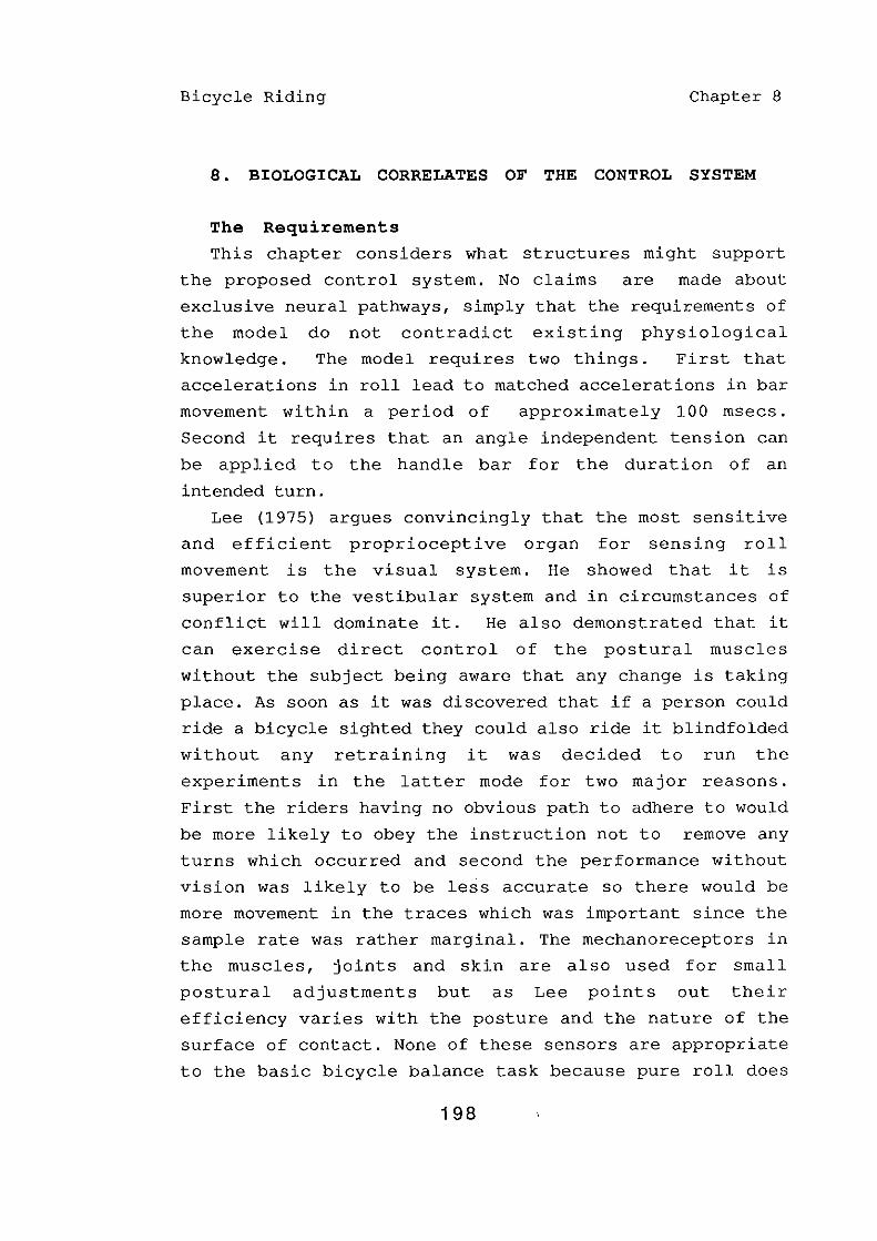
Bicycle Riding Chapter 8
8. BIOLOGICAL CORRELATES OF THE CONTROL SYSTEM
The Requirements
This chapter considers what structures might support
the proposed control system. No claims are made about
exclusive neural pathways, simply that the requirements of
the model do not contradict existing physiological
knowledge. The model requires two things. First that
accelerations in roll lead to matched accelerations in bar
movement within a period of approximately 100 msecs.
Second it requires that an angle independent tension can
be applied to the handle bar for the duration of an
intended turn.
Lee (1975) argues convincingly that the most sensitive
and efficient proprioceptive organ for sensing roll
movement is the visual system. He showed that it is
superior to the vestibular system and in circumstances of
conflict will dominate it. He also demonstrated that it
can exercise direct control of the postural muscles
without the subject being aware that any change is taking
place. As soon as it was discovered that if a person could
ride a bicycle sighted they could also ride it blindfolded
without any retraining it was decided to run the
experiments in the latter mode for two major reasons.
First the riders having no obvious path to adhere to would
be more likely to obey the instruction not to remove any
turns which occurred and second the performance without
vision was likely to be less accurate so there would be
more movement in the traces which was important since the
sample rate was rather marginal. The mechanoreceptors in
the muscles, joints and skin are also used for small
postural adjustments but as Lee points out their
efficiency varies with the posture and the nature of the
surface of contact. None of these sensors are appropriate
to the basic bicycle balance task because pure roll does
198

Bicycle Riding Chapter 8
not produce any change at rider bicycle contact points.
However during a balanced turn there will be a slight
increase in pressure similar to the sensations encountered
when a lift stops. This is a possible source of
information in judging the threshold at which to initiate
a recovery but the lift analogy should warn us that the
system has a rather high threshold in this respect since
very smooth lifts succeed in stopping without transmitting
any sensation. Thus it can be seen that for these
experiments the roll detection requirement will be
satisfied if it can be shown that an output from the
vestibular system, proportional to short-period roll
accelerations, is fed via a reasonably short neural
pathway to the gamma and alpha motoneurones of the arm
muscles in such a way as to create in them a proportional
tension without interference from antagonistic muscles and
synergistic stretch reflexes.
The Vestibular System
The vestibular apparatus is a mechanism shared by many
species. Its structure and operation have been
extensively explored and the details are described in
introductory text books. (e.g. Davson & Segal, 1978). In
order to give a quick response to out-of-balance movements
the neural connections take a characteristically short
path to the relevant motor structures. The organs are
situated in the inner ear, one on either side of the head.
Each has three semicircular canals which respond to the
relative movements between them and the fluid they
contain. These lie in three mutually orthogonal planes so
that any pair can be excited maximally by a rotation of
the head about one of the three axes. The responses are
fed via the vestibular neurones to the vestibular nuclei
where they give an integrated output defining the
movement of the head.
199

Bicycle Riding
cortex
reticular formation
Chapter 8
semicircular canal
vestibular nuclei
to spinal motor neurones
Figure 8.1 Pathways from the vestibular system to the limb muscles. Output can go either direct or via the reticular formation which is open to modification from the cortex. (Adapted from Davson & Segal, 1978)
Figure 8.1 shows a formal representation of the way in
which information about the internal arrangement of the
parts of the body is integrated with information from the
vestibular system via the reticular formation. This is a
region of the brain stem exerting a powerful influence on
the skeletal musculature and consequently an important
control-centre for the organization of movement.
There have been a number of experiments addressing the
question of direct pathways from the vestibular system to
motor control neurons. For example Eldred (1953) showed
that a powerful influence was exerted on gamma fusimotor
neurons by the vestibular system and this was confirmed in
subsequent studies by Grillner et al. (1969), while Lund
and Pompeiano (1968) showed that the extrafusal alpha
motoneurones also received monosynaptic activation from
the same regions. Lund and pompeiano concluded that only
extensor motor neurones were activated but Grillner et al.
considered that those of the flexors were also activated
via the reticular formation which has close connections
with the vestibular output.
200
Bicycle Riding
Deiter's nucleus
extensor
Chapter 8
Medi I'll 1 ongi tudi nl'll
fasciculus
Figure 8.2 Schematic representation of descending monosynaptic effects via fast conducting fibres from Deiter l s nucleus and the medial longitudinal fasciculus on the alpha and static gamma neurones to flexors and extensors acting at the knee-joint. All synapses are excitatory. (Adapted from Grillner I 1961))
They proposed the connections illustrated in figure 8.2
for the knee joint showing influences of both intra and
extrafusal efferents from Deiters nucleus, which is a
vestibular nucleus, and the medial longitudinal
fasciculus, which is the main pathway taken by the
reticulospinal fibres to the motor neurones.
The vestibular mechanism has two sorts of transducer,
the otolith organ in the utricle and saccule, and the
ampulla in the semicircular canals. Figure 8.3 shows the
general arrangement of these structures in the inner ear.
Detailed research into the output performance of the
otoli th organ has not been as extens i ve as for the
ampulla. The exact role of the saccule is uncertain.
Ablation seems to have no adverse effect on balance though
there is some evidence that visual acquisition may be
201

Bicycle Riding Chapter 8
affected. The utricle responds principally to changes in
the rolling and pitching plane.
the semi-circular canals
ampulla posterior
ampulla anterior
ampulla lateralis
vestibular --~ ____ ~---------- nerves
F i gu re 8 . 3 The semicircular canals the inner eat.
general arrangement of the and the sensory transducers in
The general form of the discharge rate is a
linear function of the effective force acting upon the
organ (Fernandez et al 1972). It should be borne in mind
that the way in which the total system integrates all the
outputs from the various transducers at the vestibular
nuclei during head and body movements is not known in
detail. However, it seems fairly certain that the main
function of the otolith organ in balance is to give a
response to the statiC relationship between the head and
the pull of gravity.
The operation of the ampulla, which responds to the
relative movement between the semicircular canals and the
endolymph they contain,
deal of research.
observations of the
has been the subject of a good
Steinhausen, following direct
cupular of the carp in 1931,
formulated the proposition that the movement under
acceleration acted as a heavily damped torsion pendulum.
(Summary in Ha11pike and Hood, 1953) . Unfortunately such a
202

Bicycle Riding Chapter 8
model predicts that the output will fall to zero for the
very short-period excitation which is the more normal
type of stimulus encountered in everyday movements.
Despite this the model was adhered to for many
leading to a dearth of experiments exploring
particular range of values. Some light, however, is
on this subject by Fernandez and Goldberg (1971).
years
this
shed
They
studied the output of selected neurons associated with the
semicircular canals of the squirrel monkey when the animal
was subjected to controlled rotations in a cage-like
apparatus. When sine-wave inputs controlled the movement
of the monkey's carrier it was seen that the response no
longer followed the predictions of the damped torsion
pendulum model. The information obtained from these
experiments was used to modify the equations, by altering
the time constants, until the predictions followed the
observed output. Using the new values they predicted the
responses to three rising half sinewave accelerations in
the range of interest. These predictions are shown in
figure 8.4. The upper graph shows the predicted response
to the three stimuli. The lower graph shows the change of
velocity for these on the same time scale to emphasise
that the vestibular system discriminates between them with
different spike rates even though they all peak at the
same maximum velocity. Although this is a prediction, not
an experimental result, it is a reasonable extension of
the findings of the paper and gives a clear indication
that the vestibular system is capable of producing a
response that is proportional to the rate of angular
acceleration. This is the sort of performance needed to
drive the projected bicycle control model.
203

Bicycle Riding Chapter 8
Response
; ('.!AihL::~_ ......... (_cana
1 output)
, J\ Normalized response 0
(spikes/sec) -1
-2
-3
Angular velocity 0 (deg/sec)
.. ;:; ... : . .. '.: :. .:. :.: .:. _.:::-.: :,' .: :.: .: . . : :', :',
\,8 htz ':l:l:
::: ..... ::. 8 htz
4 htz 2 htz
Stimulus (change of position)
Figure 8.4 Showing how the response of the semicircular canal to short period rotations discriminates between different rates of acceleration (spike response, upper graph) even though the final angular velocity is the same in each case (lower graph). (Adapted from Fernandez & G6ldberg, 1971, page 673)
The Motor System
The fine details of motor control are extremely
complex, especially in the higher animals where there is
an increasing contribution from central rather than local
sources. Every limb has a number of independent muscle
groups acting both as extensors and flexors and each
204

Bicycle Riding Chapter 8
muscle consists of a very large number of separate muscle
spindles which themselves consist of a number of separate
muscle fibres. Each fibre can be influenced by electrical,
chemical and mechanical means and the nerves that take
information from and to these fibres branch in many
different ways, so that even within a spindle var ious
groups of fibres share some nerve paths but not others.
(de Vries, 1967; Thompson, 1975; Granit, 1970).
Many findings have been obtained from in vitro
investigations of animal preparations. Sufficient
important differences of detail between animals have been
observed to make the direct extension of these to humans
problematical. In the lower
the intrafusal spindles are
animals, such as amphibians,
innervated by branches from
the extrafusal musculature whereas in mammals there is an
increasing independence of the intrafusal and extrafusal
systems (Granit, 1970). In the former case it is possible
to account for such behaviour as posture in terms of a
spinal reflex response to stretch imposed by altering
loads. In mammalian muscles, however, there are
reflex-like movements which in fact depend on intrafusal
activity and which can be maintained in the absence of
extrafusal (alpha) output (Granit, 1970). The emerging
picture is one of an extremely elaborate automatic control
which is able to make constant adjustments to the
multitude of individual muscle fibres. The balance of
flexors and extensors by alternating the recruitment of
various semi-independent muscle groups is an essential
feature of smooth continuous operation.
Automatic and Volitional Control
The degree to which such systems are automatic, that
is they depend on changes due to direct interaction with
the environment, rather than volitional control by the
higher centres of the brain, is still an open question.
205

Bicycle Riding Chapter 8
The greater complexity of the mammalian system with its
nerve tracts from the intrafusal spindles extending into
the lower brain stem and beyond makes single cell
recordings extremely difficult to interpret and these
difficulties are multiplied by the fact that all natural
movements are polyneuronal. In some systems, it is
possible to build up a fairly clear picture of the
contributions from the various parts of the nervous
system. Euler has proposed a circuit for the action of
the intercostal muscles during breathing that accounts
for in vivo performance when the air passage is
restricted. Control is shared between the spine,
respiratory centres and the cerebellum and it is evident
that since single inhalations and exhalations can be
voluntarily imposed there must also be indirect links
with the higher parts of the brain (Granit, 1970).
In an experiment by Basmajian et al (1965) a subject
learned to regulate the level of excitation from an
electrode placed in the abductor pollicis brevis of the
thumb. This was achieved by attending to visual and audio
feed-back. It is clear that volitional control of very
small muscular units is possible whatever the functional
implications might be. In general it seems most probable
that for well established actions such as breathing and
walking there is a 'proprioceptive elaboration of a
relatively simple central command alternating between
flexors and extensors.' (Granit, 1970) and that during the
learning process the higher brain functions interrupt and
redirect these established sub-systems to create new
'automatic' links which allow the new skill to become part
of the repertoire.
206

Bicycle Riding
Flexor muscle folds elbo .... PULLS BAR ~
No .... rist moyement~
joint free to rot8te
Extensor muscle str8ightens elbo .... PUSHES BAR
~ Trunk keeps
-- st8tion8r!l on bike
Figure 8.5 Showing the simple model for single arm control of the handle bar.
A Possible Control Mechanism
Chapter 8
Typical control movements are used with steering
wheels, boat tillers, aircraft joysticks etc., and take
the form of a tension in the appropriate muscle group and
inhibition of the antagonistic groups so that the control
mechanism moves to that position where the muscle tension
balances the mechanical torque. It is highly likely that,
in common with most human activities, individuals will
have a large repertoire of effective alternatives for
achieving appropriate control movements but in order to
compare the known capabilities of the motor-system with
the control demands some simplified model is needed.
Figure 8.5 shows a schematic layout for the proposed
operation of the steering mechanism. An informal riding
experiment was carried out in which the bar was held in
every strange way that could be devised. Clenched fists,
palms flat, back of the hands, finger-tips, wrists, lower
forearms etc. The only problem encountered was when
pushing or pulling very lightly with fingertips only. In
207

Bicycle Riding Chapter 8
this position the body was deliberately held back to avoid
contributions from movements of the upper trunk. With
sudden turns it felt as though one of the hands was coming
off the bar which lead to a momentary wobble. When the
load on the bar was increased by leaning
fore ward depending on whether pushing of
effect disappeared.
backward or
pulling the
Thus it seemed that since the hands themselves were
playing no part in the operation either as sensors or
actuators it was reasonable treat them here as a single
unit together with the wrist and forearm. In order to
turn the front wheel the rider must alter the relative
distances from the tips of the handle bars to the saddle
and since it assumed that the lower trunk and legs do not
normally move for steering purposes this is the same as
altering the distances between the forearm extremities and
the hips. This movement could be aChieved in several ways.
The arms could be kept the same length and the upper trunk
swivelled, Or the trunk could be kept still and the arm
lengths altered by changing the angles at the shoulder and
elbow.
Although either arrangement is possible from the
purely mechanical aspect a simple experiment suggests
that the postural reflexes give a more restricted choice.
If one sits in a chair in front of a table and grasps the
edge with the arms slightly bent at the elbow in an
approximate imitation of the bicycle riding position
(figure 8.6), an attempt to rotate the upper trunk by
consciously changing the length of the arms produces only
a change in arm tension. In order to alter the trunk
position it is necessary to intentionally 'twist the body'
in which case the arms just follow the movement.
208

Bicycle Riding Chapter 8
Figure 8.6 The simulated riding position.
If the chair is moved a little further back so that
the weight of the upper trunk is partly carried by the
table, as in the drop-handle bar position, the shoulders
can still be twisted voluntarily and, despite the extra
load they are now carrying, the arms move to accommodate
this change. Allowing one hand to slip suddenly from the
table edge leads to virtually no alteration in the trunk
position, the full weight being taken by changes in the
supporting muscles. This sudden shift of weight from both
shoulders to one must produce a twisting couple on the
upper trunk but no appreciable movement is noticed. This
implies that there is a well established reflex that
controls both the fore and aft and twisting movement of
the trunk to oppose externally applied forces. It will
therefore be assumed, in the interest of establishing a
simple model for discussion, that control of the bar is
effected by altering the tension in the elbow joint
muscles and that the forces generated are transmitted
entirely to the steering bar.
Also in the interests of simplicity it will be assumed
that control is exercised by pushing and pulling on the
209
Bicycle Riding Chapter 8
bar with one arm only, leaving it open as to whether the
other arm passively follows or makes a similar shared
contribution. It may be noted in passing that, although
one-handed riding is quite normal, most riders prefer to
have two hands on the bar for difficult manoeuvres,
suggesting that there may be some operational difference
between one and two handed riding.
Resting Tension.
In the simplest of terms what is required for steady
dead-ahead riding at speed is a situation where the
muscles operating around the elbow joint are fully
relaxed, allowing the handle bar to follow the movements
of the autocontrol. However, it is necessary to propose
some slight resting tension in order that the muscles will
be in an 'alert' state to respond to control demands. This
stable tension is the 'tonus' of the muscle defined by
Basmajian (1962 p41) as ' .. determined by both the passive
elasticity or turgor of the muscular (and fibrous) tissues
and by the active (though not continuous) contraction of
muscle in response to the reaction of the nervous system
to stimuli.' Thus the flexor and extensor muscles will be
set at some steady low value which holds the elbow joint
at a particular angle in the absence of an external load
but which will allow movement under such a load without
the relative tensions changing. This slight resistance to
movement due to tonus will act as a high-frequency damper
in the steering system.
Muscle Control
The motor system has to fulfil three requirements.
First it must provide a stable platform from which precise
control movements can be made. Second it must apply an
angle-independent torque force to the handle bar to
produce a turn. Third, in the low autostability case, it
210

Bicycle Riding Chapter 8
must move the handle bar so that its angular acceleration
continuously follows the acceleration in roll.
In animals with no independent neural circuitry to the
intrafusal spindles the 'stretch reflex' provides a crude
'constant length' device. The role of the mammalian
spindles in the control of muscle length is by no means
fUlly understood; but there is no doubt that the stretch
reflex to prevent changes in length is one of the
available functions. Without going into any greater detail
it can be seen that the requirement outlined here for
stabilizing the trunk is consistent with what is currently
known about the system.
When there is appreciable torque in the steering head
from the bicycle's autocontrol the requirement is for the
rider to allow this to operate and at the same time add a
further torque force for additional control. When the
elbow joint moves to accommodate the movement of the bar
under the resolved rider/machine couple the muscle lengths
will change. The length/tension ratio of the flexor and
extensor muscles must be set to constant values so that
their difference remains the same despite these changes in
length. That is there must be no stretch reflex.
All the early work on muscles encouraged the idea that
they achieved their postural tonus via a stretch reflex
mechanism. This meant that when a muscle had achieved a
set length due to alpha excitation any increase in length
caused by some outside force such as change in body
loading would automatically lead to the recruiting of
extra fibres to increase the resistance and hold the
position; Obviously such a system will not answer for the
purposes of bicycle control. Later research has shown that
in mammals at least the intimate control of the excitation
values in the main alpha neurons of the muscles is subject
to influences from both the intrafusal spindles and the
golgi tendon organs. The afferent output of the
211

Bicycle Riding Chapter 8
intrafusals can be made selectively sensitive to length
and rate of stretch or inhibited by changing the values in
the static and dynamic efferents to these units. This
output can be directed to excite or inhibit synergistic
and antagonistic muscle groups remote from the detection
site. The input and output connections to the intrafusal
spindles have branches up to the brain and consequently
the motor muscles are no longer tied to a simple stretch
reflex. Response for various combinations of afferent and
efferent excitation can produce a great variety of control
responses.
As long ago as 1909 Sherrington reported a condition
in a decerebrate cat where the extensor (vastocrureus) of
the leg could be moved to various positions by the
experimenter. Previously it had been thought that limbs
would be either completely relaxed, in which case they
would fall back under gravity if displaced, or rigidly
held in some position against gravity, in which case
attempts to move them would lead to a stretch reflex
opposing the change. The condition observed by
Sherrington, which
fully explained
he termed 'plasticity' has still to be
but it is now apparent that the
independent control of the intrafusal spindles and golgi
tendon organs in muscles allows a large combination of
autogenetic and antagonistic activity which could account
for a condition where the reflex due to external
stretching was irihibited (Matthews 1972, pp 443-445). The
'alert' no-signal condition proposed in the paragraph on
resting tension above is similar to the plastic condition
observed in the cat preparation, although since the arm is
supported at handle-bar and shoulder the resting tonus
need be nothing like so great as that required to hold the
weight of the limb against gravity. Figure 8.7 illustrates
an experiment by Buller and Lewis on the length-tension
curves of the soleus muscle in the cat. The curve shows
212

Bicycle Riding
the change in
(abscissae) when
Chapter 8
tension (ordinate) against
the muscle was subjected to
length
a full
'tetanus' excitation (described in Granit, 1970).
t 1200 e n 5 i o 1000 n (gms)
800
length (mm) 4 8
---a-._a_a_a, a..--II .. II-II ........... _
12 16 20 24
Figure 8.7 The relationship between length (abscissa) and tension ( ordinate ) of the soleus muscle in a cat when subjected to full tetanus excitation. (Adapted from Granit, 1970, fig. 10, page 23)
The implication here is that if this muscle, holding a
load of say 1000 grams at a length of approximately 4mm,
was then shortened by some external force to 3mm then the
force generated would fall to 900grams and in the absence
of any other input would continue to collapse since it
could no longer support the initial load. If however the
same test was applied on the flat part of the curve
between 7mm and 20mm the tension would not alter and the
new position would be held. Of course this experiment
takes no account of what the antagonistic muscles are
doing at the same time, nor of the effects of altered
instructions from higher levels of organization as a
result of the changes in excitation of the fibre
afferent-s, but it does illustrate that the internal
organization of this muscle can exhibit the quality of
constant tension for changed length. Marsden et
213

Bicycle Riding Chapter 8
al. (1971) describe an experiment in which an unexpected
opposition to the voluntary movement of a subject's thumb
was suddenly introduced. In the normal state this
resistance led to an automatic increase in the tension of
the driving muscle to maintain the intended rate. When
however the thumb was anaesthetised by local injection
there was a reduction in the rate of response, indicating
that the tension had not altered. This finding is usually
quoted as an instance of the contribution of the jOint and
cutaneous sensors to this sort of 'reflex' since the
muscle that does the driving is in the arm not the
anaesthetised thumb. However the point here is that the
subject is producing the kind of movement required by the
control model for the operation of the handle-bar. In the
case quoted the feedback seems to have been blocked by the
anaesthetic. In the case of the bicycle it would have to
be as a result of some sort of organized inhibition of the
spindles and/or golgi tendon organs.
Thus it can be seen that the human neuromuscular system
is capable of producing a constant tension in a muscle
independent of changes in length and that volitional
control over small isolated muscle units has been
demonstrated. This is sufficient evidence to justify the
claim that holding an angle-independent tension to produce
turns is consistent with what is known about the motor
control system.
The Roll Induced Movement
The final requirement is to produce a continuous
angular movement of the handle bar in response to the
vestibular output. There are many functions in mammals
that show a fine control of position which can only be
explained by independent spindle action. A good example
being provided by the demonstrations by Euler that the
desired 'tidal volume' of the lungs is controlled by the
214

Bicycle Riding Chapter 8
length to which the intercostal intrafusal muscles are
stretched in breathing (in Granit, 1970) Thus the
essential neural connection to adapt the existing system
for roll-follow control is to take the rate of change of
excitation in the vestibular system caused by rates of
roll and apply it via some multiplier to the tension
values in the arm muscles. It is not intended to imply
that the implementation of such a link is in any way
simple. The extremely complex polyneuronal nature of any
limb movement is such that comparatively simple movements
in the large muscle groups must be translated into a vast
array of 'messages' to each of the individual muscle
spindles involved.
An experiment by partridge and Kim (1969) provides
an interesting observation of a very similar system
actually operating in the cat. They recorded the isometric
tension in the triceps surae muscle of a cat during the
sinusoidal excitation of the ampullary nerve bundles of
the vestibular system. Between a wide range of frequencies
the tension in the limb moved in sympathy with the
oscillation of the stimulus, with a conduction delay
of 15 msecs which is several times faster than that
observed in the human rider. This is exactly the sort of
arrangement required to operate the control model.
Comparison with Postural Control
There is a literature on postural control as distinct
from motor movement because to some degree posture is seen
as being controlled by local reflexes rather than a
centrally controlled organization. The problem is that
studies of posture in man show evidence of central
contributions and complex responses for simple bipedal
balancing tasks at latencies below the minimum recorded
for voluntary movement. Recording exactly what every limb
is doing during natural movements is extremely difficult
215

Bicycle Riding Chapter 8
and it is all too easy to misinterpret local motion
because the whole action has not been captured.
Consequently it is usually very difficult to be quite sure
what role muscles are actually playing in a complex
movement. There is evidence that sequences of postural
actions are anything but 'dumb' local reflex responses,
but at the same time their speed of action at the lowest
level of the hierarchy argues that reflex like processes
are being recruited in the responses. Since learning to
ride a bicycle necessitates recruiting fast responses for
lateral balance it is very likely that there is a link
between standing postural control and bicycle control. The
proposal that pushes superimposed upon and temporarily
disrupting the underlying continuous balance induce
desired changes in lean
balance
blocks
during motion.
angle also speaks to
The sprinter on his
bipedal
starting
is so
represents an
far displaced
extreme example. The centre of mass
from the support point that only a
very high rate of acceleration will prevent a fall. By
disturbing the autonomous balance system the higher centre
of control forces a response which achieves its
requirement without further contributions. Two sets of
exploring the sequencing of
standing balance will be used
responses in
to illustrate
experiments
maintaining
some of the common points between the bicycle task and
posture control.
Nashne:r's Pll!ttform Tasks
Nashner (1976) conducted a series of experiments in
which subjects stood on a platform which could be
translated in the antero-posterior (A-P) direction and
rotated to give a 'toes up' (dorsiflex) or 'toes down'
(plantarf1ex) movement of the ankle joint either
independently or simultaneously. Changes in body sway and
the torsional forces applied by ankle musculature were
216

Bicycle Riding Chapter 8
measured during platform movements. Nashner' s interest
was in the possible role of reflex responses in the ankle
for posture control. Seven of the twelve subjects made no
rapid compensation for the mildly disturbing changes
induced but brought in appropriate ankle movements after
about 200 msecs. These responses were considered to be of
visual or vestibular origin so the focus was on the five
who made fast reflex-like responses.
It was clearly shown that changes in ankle angle
induced muscle responses in the smaller group, even when
they were inappropriate and caused unwanted sway. When the
platform was moved backwards the subjects made a toes down
movement after a latency of approximately 120 msecs to
oppose the induced foreward sway. When the platform was
rotated in the dorsiflex direction without any translation
the subjects responded with a plantar flex movement which
was inappropriate and gave a self-induced sway backwards.
After three or four trials this reaction was adapted out
and then resumed when the conditions were altered to make
it appropriate again. This sort of reflex movement is
termed a Functional Stretch Reflex (FSR) as opposed to the
faster myotatic response, which has a latency of 45-50
msecs. No myotatic responses were recorded in any of the
experiments.
In his discussion the author proposes that both the
fast reflex action of the smaller group and the delayed
visual or vestibular response of the larger, fit into an
hierarchical model of postural control in which the
cerebellum exercises control over the gain of reflex
responses to achieve the desired effect. He quotes two
different models for the organization this control.
Welford (1974) suggested that the central process adapts
an internal 'model' of appropriate responses to cope with
unexpected changes whereas Pew (1974) suggested that when
faced with an inappropriate response the system suppresses
217

Bicycle Riding Chapter 8
the existing action to give more time to assess what was
happening before producing a new response. Nashner
suggests that these two models offer possible explanations
of the difference between the fast responding and the slow
responding subjects with the slow subjects using the
latter strategy and the fast ones the former. Even when
one of the slow subjects was told exactly what was
happening he was unable to override the inappropriate fast
response, but it is of course quite possible that a longer
period of training might have allowed a conversion
eventually to the more flexible system. Several subjects
with deficits of the cerebellum were tested on the same
task and showed little ability to adapt their fast
responses in the inappropriate task.
These two models can be directly related to the problem
of learning to ride a bicycle. The point about the bicycle
task is that it appears on the surface to be a
navigational problem, like riding a tricycle, but it
carries with it a postural-like balancing element which is
intimately tied in with the former. When the rider first
tries to steer for direction only there is a strong out of
balance effect. It can be assumed that the initial
response will be that already established for postural
balance, in the same way that Nashner's 'fast'
moved their ankles inappropriately. That is,
subjects
the body
will be rotated away from the direction of fall in an
attempt to keep the weight within the support platform.
In many cases the outside foot will in fact be moved from
the pedal to the ground to ensure stability. The first
thing the rider must learn is to suppress this
inappropriate response and replace it with a handle-bar
movement into the fall. Once this has been established
the cerebellum can exercise its gain control of the arm
action to achieve an acceptable balance between stability
and power. The fact that Nashners' 'fast' subjects
218
Bicycle Riding Chapter 8
suppressed the inappropriate ankle response in typically
three or four trials shows that such adaptation is part of
normal balance and goes a long way to explaining why
children can learn to ride a bicycle so quickly.
The difference between the myotatic and FSR response,
(70-75 msecs) presumably reflects the extra time needed
for the sensory pulse to ascend to the brain and the
instruction to return. The difference in the latency
between the slow and fast subjects, 200 msecs as opposed
to 120 msecs, seems to be a function of different basic
strategies and it is not necessary to assume that the slow
subjects would be irrevocably committed to such a latency
in different circumstances. That is once the connection
between the vestibular or the visual system has been well
established there is no reason why the latency should not
reflect the time taken for the one way journey from the
detecting site in the head to the arms. In bicycle riding
the information for driving the response comes from the
inner-ear Or the eye which, unlike the ankles in the
sources very near to the cerebellum. platform task, are
Consequently there is no need to allow time for returning
information. Partridge and Kim's cats, mentioned above,
had a system delay of 15 msecs, so there seems to be no
objection to the 60-120 msecs phase delay observed in the
runs. It is also possible that the difference in delay
between the two riders was due to a predisposition to
'fast' or 'siow' styles of response. Certainly the slow
responder was the more skilled rider of the two and had a
wide experienbe of other balance skills such as skiing and
surfsailing.
A later paper Cordo and Nashner (1982) provide further
evidence of activation of controlling muscles in both the
leg and the arm at latencies below that elicited by purely
voluntary movement.
balance system is
They also show that the postural
anything but an unadaptable local
219

Bicycle Riding Chapter 8
reflex, and that the site of action can be switched
without practise when this is appropriate to maintaining
balance.
In a series of experiments subjects made arm movements
or reacted to arm pulls which on their own would have
upset the postural balance. By recording muscle activity
in the arms and legs on a common time base it was shown
that potentially disturbing arm movements were either
preceded by appropriate leg movements or were held at a
low level until the leg movement had been initiated. It
was evident from their findings that the instruction to
pull or push with the arm was interpreted in such a way
that activity in the legs was first recruited to 'set up'
the situation so that when the arm movement came it
applied the mass of the body to the point of application
rather than swaying the body out of balance. It was also
shown that when movement of the arm was more appropriate
to keeping balance the leg response was suppressed and the
arm moved instead.
Of particular interest to the proposed bicycle control
was an experiment where the subject stood on a platform
which oscillated 10 degs 'toes up' and 'toes down' in a
continuous 0.1 Hz cycle forcing the subject to make
compensating movements of the postural muscles to keep
balanced. At a signal the subjects had to pull or push a
handle mounted at waist level. Cordo and Nashner' s
interest was the slight increase in reaction time of both
the biceps and gastrocnemius muscles compared to the same
task when the platform was stationary. Although the
continuous movem~nt to maintain balance was in the leg the
superimposition of an additional burst of activity at a
mean latency of 127 +- 38 msecs is exactly the sort of
activity required of the arm in control of the
destabilized bicycle with comparable delay.
Another interesting finding was the way that balance
220

Bicycle Riding Chapter 8
control was immediately transferred to the arm from the
leg when this was the most appropriate movement. Such
instant transfer of activity to a different site is
exactly what is envisaged during the initial learning
task. Cordo and Nashner's subjects already possessed the
necessary organization to select the arm as the
appropriate site of action. The naive bicycle rider
apparently does not and must learn it in the same way that
the experimental subjects had originally to learn theirs.
The voluntary response time from the biceps was
measured as 155 +- 37 msecs, but during the pull and push
trials this fell to 66 +- 12 msecs and 73 +- 24 msecs
respectively. This supports the earlier claim that when
acting as a coordinated system the response time of
muscles cah be much faster than the latencies which are
elicited by voluntary movement, and consequently it is
argued that the 60-120 msecs phase delay discovered in the
continuous roll/bar control of the destabilized bicycle is
quite in line with this class of movement delay.
Lee's Swinging Room
The final reference to the postural literature concerns
a set of experiments by Lee and Aronson (1974) and Lee and
Lishman (1975). In the first experiments the authors
induced inappropriate postural responses in standing
infants and later in adults. When a 'swinging room'
produced the sort of visual information usually associated
with body sway, even though no change in posture was
present, subjects tended to make compensatory movements
which led to loss of balance. This effect was stronger in
the infants but was also present in the adults to a lesser
degree.
In the second paper the authors concluded, again using
their swinging room apparatus, that vision was the primary
source of postural information for standing balance.
221
Bicycle Riding Chapter 8
Subjects were induced to respond to room movements as
though their balance had been upset. In one experiment
the room was moved back and forth over a distance of 6 mm
in a regular sinusoid with a period of 4 secs. The
subjects were briefed to ignore any room sway but a record
of body movements showed that they were swaying with the
room even though they reported that they had not moved.
The paper shows a reproduction of the room and subject
trunk velocities over a period of about 50 secs. These
measurements were made from analogue pen traces and no
digitized version was recorded, however the phase
relationship between the two traces on the page is
correct. (Lee, D.N., personal communication).
It is obvious that the visual stimulus must have been
the relative movement between the room and the subject and
that the subject's movement as shown by the trunk trace
must be subtracted from the room movement to obtain this
relative motion. The events interact in a loop. The room
sways and causes the subject to induce a trunk sway to
match it as though there had been a postural change. This
at once effects the relative movement between the subject
and the room and leads to further changes. A casual
examination cannot tell us how much the vestibular system
contributes to the observed motion but the authors showed
that movement with the eyes shut was greater than the
movements induced by the room implying that the visual
information gives a greater accuracy in maintaining
balance.
There are close links between this balancing task and
the bicycle riding task. In both cases the underlying
action seems to be outside the conscious control or
knowledge of the subject. In the destabilized bicycle task
the vestibular activity appeared to be controlling the
handle-bar responses and in the postural task the room
movements appeared to control the body movements. In both
222

Bicycle Riding Chapter 8
cases the control seemed to be almost direct. In an
attempt to learn more about the detail of the form of
control in the room swaying task the curves published in
the paper were used to obtain the relative velocity and
acceleration movement between the body and the room on the
same time base.
The Trace Differentials.
Simple measurements on the traces given show that the
trunk velocity has a mean phase lag behind the room
velocity 0 f 0.75 secs with a maximum of 1.45 secs.
However it is the relationship between the trunk movement
and the relative movement of the room which is the more
important so the traces were enlarged to double the size
on a photocopier and then digitized using a PMS Graphbar
sonic bit-pad. Approximately 300 sample points were taken
of each trace giving a density of about 6 points per
second, or about 25 points per wave. The two records were
registered by interpolating between points to give values
at equal step intervals. The trunk velocity was then
subtracted from the room velocity to give the relative
velocity between them and this curve was differentiated by
taking the local slope between the values immediately
before and after each point. These three curves are shown
on the same time base in figure 8.8. The X axis has been
expanded so only half the run is shown. We can see that
the relAtive velocity is a regular wave with the same
period as the trunk velocity with a phase difference of
about 90 degrees or 1 second. Since this is the
information driving the response it is, as expected, in
advance. The relative acceleration is much noisier and it
is not possible to know how much of this comes from the
rather coarse level of recording and transformation.
223

Bicycle Riding
trunk veloclty
relative velocity
relative accln.
10 secs
Chapter 8
Figure 8.8 Actual trace of the trunk movement caused by a gently oscillating visual stimulus. (Adapted from Lee &
Lishman, 1975, page 87).
Possib1e Contro1 Systems.
A closer look at what sort of systems might control
standing balance and be disturbed in the manner shown in
the Lee and Lishman experiments shows that the problem is
complex and leads to the caution sounded above about
drawing simple conclusions from the traces of trunk and
room motion. In order to explore possible control systems
the bicycle simulation was modified to reproduce a much
simplified version of the standing task. The following
dimensions were used to represent a typical person: weight
160 lbs with a rigid body 6 feet tall having the mass
evenly distributed along its length with the centre of
mass half way at 3 feet. The eye level was 5.5 feet and
all movement was assumed to be around
that in real life
the ankle joint. It
people have a much is quite obvious
wider choice of movements with which to respond to
locked the foot vertical imbalance. With the ankle joint
gives quite a large support base in the fore and aft
direction and any disturbing push would lift the toe or
heel and give a strong correcting couple. Movements of
the big toe provide a powerful couple very fast and it is
224

Bicycle Riding Chapter 8
known that loss of the great toes in an accident does give
balance problems. It is very likely that the ankles, knees
and waist joints all act together in a synergistic
response which would have important effects on the way the
centre of mass moved in relation to the support point.
However the fact remains that very small movements of the
swinging room produced body sway responses so it is
evident that the subjects in the experiment were primed to
make active responses to disturbances and not just relying
on the passive stability conferred by a locked ankle
joint.
The problem for the standing person is this: any
displacement of the centre of mass from directly above the
support point leads to an increasing rate of acceleration
into a fall. The subjects in the swinging room experiment
only deviated 5mms either side of the upright so if the
height of the measuring device on their backs was about 4
feet they were only swaying through an included angle of
less than 0.5 degrees. Thus we can see that very small
changes are significant and the performance of the
simulation shows that it needs to be, if it is to keep
control. Any active control must first sense a fall and
then oppose it. The longer it leaves the correction the
more effort it needs. If it produces a much bigger
correction than is needed it will cause an acceleration
back over the zero position and then will be faced with a
worse situation on the other side. This will be repeated
in increasing oscillations unt il one fails to reverse.
Thus we can see that the problem is the same as that
encountered in the bicycle control. Discrete corrections
are far too unstable to be realistic, so the sensed rates
of movement must be fed back with a gain which is big
enough to contain any expected disturbance but not so
great as to produce a diverging oscillation. Any long
delay between sensing and implementation will increase
225

Bicycle Riding Chapter 8
instability and therefore limit the amount of gain which
can be used. If only acceleration is fed back the velocity
will not be removed, if both the velocity and acceleration
are fed back then any angle which accumulates during the
operation will remain and this will lead to a further
increase in the falling couple. Stability is typically
achieved by actively oscillating about the zero point.
Control of limb joints must take place via changes in
length of muscles. Extensor and flexor muscles must work
in sympathy and movement is possibly specified by giving a
common set point at which the tensions are equal. However,
as far as the joint movement is concerned this is received
as a torque couple and that is how such changes were
modelled in the simulation. The movement around the ankle
was obtained by working out the weight couple from the
displacement of the centre of mass from the support point
and adding to it any muscle torque specified by the
control system. The room movement was modelled so that
relative movement between it and the person could be
found.
First the simulation was given a feed-back control
system which feel. the velocity and acceleration of the
trunk into the ankle joint opposing any fall. The gain was
trimmed so that it could restrain the natural fall to
somewhere the same as that seen in the experimental
traces, ie. about 0.25 degrees in one second. The
unrestrained fall rate will give about four times this
dispersion in the same time period over the same angle
range. Now the Lee and Lishman demonstration shows that
when the room moved the person responded as though he had
swayed so the control was changed to feed in relative
movement between the room and the eye position rather than
the actual body movement. The result was that initiallY
the control torque worked in the same direction as the
weight couple and an acceleration much greater than the
226

Bicycle Riding Chapter 8
free fall case was the result. With the gain available
this system was unable to contain the initial fall and
went out of control at the first dispersion. If the gain
was increased so that the fall could be checked the system
became unstable going into an ever increasing divergent
oscillation. In real life it is evident that dangerously
excessive accelerations invoke a different level of
response, such as putting out a foot or raising an arm. In
any case the experimental subjects did not behave in this
way but contained the fall within 0.25 degrees.
Secs Relatiye Room accln. yeloc. yeloc.
16
14
12
10
8
6
4
Figure B. 9 Simulation of standing balance with trunk acceleration being driven by feedback of both vestibular and visual motion from the swinging room. A short pulse of 0.44 secs duration has been put in to the right at 9.0 secs.
Evidently what is needed is some sort of restraint on
the rate of actual fall induced by the false room
information. The vestibular system would not be subject to
the deceptive movements of the swinging room but would be
measuring the actual fall and thus could be a suitable
source of information for such a restraint. The question
then is, what happens if the control is fed both the
visual and the vestibular changes? This is where the
227
Bicycle Riding Chapter 8
model comes into its own as it is certainly impossible to
visualize what the effect of mixing the two inputs would
be on the control output without one.
Figure 8.9 shows the output when the true velocity and
acceleration in fall is fed into the control together with
the relative velocity and acceleration due to the
deceptive room movement. The result is a controlled trunk
velocity with the same period as the room velocity which
is exactly what we see in the real traces. The delay
between these two in the simulation is about 0.5 secs as
opposed to the actual mean lag of 0.7 secs but this can be
increased to the same value in the simulation by
introducing a delay into the control routine.In both this
and the bicycle simulation it was demonstrated that
putting velocity and acceleration information into the
control leaves any accumulated angle untouched. In the
bicycle case this left a residual turn, which is stable,
but in the standing balance case it leaves and angle of
lean which produces a disturbing weight couple. Since the
simulation is controlling on velocity and acceleration
only, the angle gradually accumulates as can be seen by
the way the mean of the vertical angle trace in figure 8.9
is moving gradually left.
The human can easily alter the relative position of its
parts to achieve a change in the relationship between the
total centre of mass and the support point, something the
simulation has no power to do. However another method of
dealing with residual angles is to do what the bicycle
riders did and put in a short push pulse to oppose them.
Just to emphasize that a short push, such as might be
administered by a rapid movement of the toes, will have
the same effect as it did on the zero-stable bicycle, a
single pulse lasting just under half a second has been put
in at the nine second mark, and is shown by the arrow.
This added pulse pushes the mean of the vertical angle
228

Bicycle Riding Chapter 8
oscillations back towards the zero line but leaves the
basic characteristic unaltered.
In the actual trace the trunk velocity has a definite
tendency towards a triangular shape. It could be argued
from this that the underlying control is putting in a
fairly steady rate of acceleration between peaks and
changing sign rapidly at each of them. If this was the
form of the control then the focus of interest would be
what unique events occur in the stimulus immediately prior
to the sign changes to cause them. Candidates here might
be the rising relative velocity which triggers the change
when it exceeds some threshold value Or possibly the rise
in the relative acceleration although this trace is much
messier and therefore less unique. Secs Trunk Relative Room
angle veloc. veloc.
4
3
2
1
Figure 8.10 Simulation of push control for standing balance as described in the text. Trunk angle varies between plus and minus 0.3 degrees. The original room velocity has been put in for reference.
However there are a number of difficulties which appear
when such a system is run on the simulation. Attempts to
control by pulse inputs alone lead to diverging
oscillatory instability. It is certainly possible to keep
control by imposing short pulses on an underlying
229

Bicycle Riding Chapter 8
continuous feed-back whenever some angle threshold is
exceeded. Figure 8.10 shows this working with pulses of a
nominal value of 4.5 applied over a period of 0.36 seconds
whenever the vertical angle exceeds a set threshold value.
The difficulty is that the period of oscillation cannot be
much increased without losing control. The period of the
real trace is 4 seconds with an angle dispersion of about
0.3 degs. In figure 8.10 the initial fall to the left
under the restraint of the continuous feed back is at
about the same rate and reaches about the same angle. At
this point a push which is strong enough to make the
angle cross the centre line immediately reduces the period
to about 1 second as shown in the figure. If it is reduced
until the initial rate of reversal is nearer to the
recorded 4 secs period then the centre line is never
reached. If the length of the pulse is increased in an
attempt to keep the reversal going there is an interaction
between the contihuous feed back and the long pulse and
the trace starts oscillating about a mean angle which
again does not cross the centre line. Only short pulses
can be used to influence the continuous system without
altering its basic characteristic. The inability to
increase the wave period is due to the natural frequency
of the oscillation of the trunk about the ankles assumed
in the model. As has already been mentioned it is possible
that a correlated movement of the body sections might make
large changes to the effective radius of gyration and thus
alter the natural frequency. It is evident that more data
would be needed before a model which might produce a
solution could be constructed and at present the
triangular shape of the trunk velocity remains
unexplained.
Although the model is a very simple one it does help us
to understand several interesting properties possessed by
such a system. If the natural control achieves this sort
230

Bicycle Riding Chapter 8
of stability by locking the ankle joint and relying on the
passive stability of the foot it would not have responded
to the swinging room. Active balancing of a standing body
around such small angles as half a degree displacement
involves almost inevitably some sort of continuous feed
back about the rate of sway. If there is too much power
the characteristic will be a diverging oscillation. If, in
the swinging room experiment, it is supposed that the
subject is under the control of visual information only
then a gain appropriate to normal conditions would be
unable to contain the sway induced by the false movement
of the room. It further shows that if the conflicting
information of both the vestibular and visual channels is
added together so that both are making equal contributions
then the behaviour of the model in the presence of the
swinging room is in many respects the same as that of the
actual recording. A much more detailed record of such
movements would be necessary before a similar analysis to
that done on the bicycle could be carried out but in the
interim it can be stated with some confidence that
standing balance control seems to face the same class of
problem as that for riding the destabilized bicycle and
that as far as can be judged from the rather sparse
information given in this paper humans set about solving
this problem in much the same way using the same basic
neural equipment.
The aim of the bicycle study was to find out the
minimum conditions necessary for control and because of
this the trials were carried out with the subjects
blindfolded. Unfortunately lack of time prevented any
trials with sighted subjects so no comparison is possible
as a series of cal ibrated runs wou ld be needed to
determine whether there was any difference in the angle
control when visual information was available. However
the general performance of the riders seemed exactly the
231

Bicycle Riding Chapter 8
same under blindfolded or sighted control and a study of
wheel tracks showed the same short and long period
oscillations were present under both conditions so it
looks as though a continuous input for angle is not used
when sighted. It would however be very interesting to be
able to ride a bicycle within a large swinging room to see
if the resulting performance was consistant with the
visual information replacing Or combining with the
vestibular input. All that can be said for sure from the
bicycle experiments is that loss of vision caused a
minimum of disruption to the established sequence of
responses and surprisingly did not 'feel' subjectively any
more difficult than normal riding. On balance this
finding together with the analysis on the Lee and Lishman
data suggests that the vestibular and visual information
are both available and under normal circumstances will
both give the same input. The complete loss of one leads
to the other taking over but the distortion of one in a
'deceptive' manner leads to an output which is consistent
with an addition of the two inputs.
Summary
The model proposed for control of the bicycle requires
that the upper trunk of the rider is held in a constant
relation to the lower trunk and consequently the machine,
during control movements. The arms must produce either
steady angle-independent tension loads on the handle bar
for turns with full bicycle autostability or short period
o%ff pushes when this is weak or
supply a continuous movement
absent. They must also
following the roll
acceleration when machine autostability is below some
threshold value on which the directional pushes are
superimposed. Although none of these functions has been
demonstrated specifically for the bicycle, it is argued
that the system as understood at present clearly has the
232
Bicycle Riding Chapter 8
capacity for all three and that the sensory and motor
performances revealed in other balance tasks is of the
same general type as that required for the successful
performance of the proposed bicycle control.
233

Bicycle Riding Chapter 9
9. THE ORGANIZATION OF CONTROL
Introduction
The enquiry so far has shown in some detail how the
handle bar of a bicycle is moved to achieve control. This
knowledge will now be related to the existing theories of
motor skill, already discussed in chapter one, to consider
how the rider might achieve control in terms of internal
organization.
The Essential Ingredients of Control
Because the bicycle is so unstable only a very limited
number of systems will satisfy the control requirements.
The autostability built into the machine by virtue of its
design removes the need for any additional inputs to
achieve basic roll stability when travelling over some
critical speed. In this condition an angle-independent
pressure on the handle bar produces a stable lean
proportional and in the opposite direction to the push.
This results in a turn in the direction of the lean and
proportional to it. Upright running is restored by
removing the pressure. Transient disturbances, such as
surface irregularities, will lead to changes in the
direction of running but roll divergence will be
automatically removed. Steady disturbances, such as side
winds, will lead to corresponding turns which can be
countered by a continuous pressure on the appropriate
handle bar. Anything which interferes with free rotation
of the steering head under the influence of the
autostability torque will cause loss of roll stability.
As the speed falls below the critical value the
autostability forces will fail to contain roll divergence
234

Bicycle Riding Chapter 9
and unless prevented the bicycle will fall into a turn to
one side or the other from which it will not recover.
There is a transient range of speeds within which the
autostability response can be enhanced by rolling the
frame in the direction of fall. Frame rotation is induced
when the upper part of the rider's body is rotated in the
opposite direction, that is against the fall.
At very low speed the autostability fails to make a
significant contribution and in the absence of any other
inputs the bicycle will fall rapidly in the direction of
the first roll departure. In this speed range riders
are observed to move the handle bar angle at a rate which
is a multiple of the roll angle, with a short phase-delay.
The essential difference between this and the machine
stability control is that it does not respond to absolute
angle as well as roll rate. The consequence is that, in
the absence of any further control inputs, lean angle
errors will accumulate causing the bicycle to go gradually
into a turn from upright running.
The absence of continuous absolute angle control and a
longer delay in the human system, also leads to a
difference in the effect of directional control movements.
An attempt to use the steady steering pressures described
above will give a rapid increase in roll rather than a
steady turn. Directional control is now achieved by
single short-period pushes, timed to allow the rather slow
response to take effect. A single push produces an
oscillatory rate of roll away from the side of
application. A moderate push will reverse this and send
the mean of the oscillations back towards the upright from
where it will gradually oscillate either back down in the
same direction or over on the other side. Straight
running consists of a series of gentle oscillations about
the upright at the natural frequency of the system, with a
restoring push whenever the lean angle exceeds some
235

Bicycle Riding Chapter 9
threshold value.
Navigational control, that is steering the bicycle in
relation to the environment, must always entail movements
via the control systems described above. In normal
conditions a turn will be demanded by a continuous push on
the side opposite to the desired turn. In the low speed
case this must be modified to separate start and stop
pushes. In the abnormal case of 'no-hands'
is effective only on bicycles with good
riding, which
autostability
characteristics, a turn is achieved by a strong roll of
the upper body away from the desired direction of turn.
Even when riding normally such body leans will enhance any
existing autostability forces. Apart from these
limitations, navigational control poses the same problem
as that found with other vehicles and is not part of this
study.
The Applicability of Existing Theories
The relationship between existing theories of motor
performance
riding will
and what has been discovered about bicycle
ndw be considered. There seems to be no
objection to applying a stimulus-response interpretation
to the basic zero-stability control loop. The continuous
change in the controlling muscles follows the vestibular
output without interference from any higher level. The
steering pushes do not replace it but are added to it. A
stimulus-response view might also be applied to the
apparently automatic removal of lean during straight
running on the destabilized machine. Whenever the angle
of lean reaches a particular threshold a recovery push is
initiated, one state leading automaticallY to the next.
This theory is not very helpful when the initial
acquisition of the skill is considered nor is it any use
when considering why a steering push is introduced for
navigational purposes.
236
Bicycle Riding Chapter 9
Motor Programs
An open-loop motor program approach cannot deal with
the intimate relationship between roll acceleration and
bar response in the destabilized control loop. The
bar rate follows the roll rate in detail and the
continuous feedback of roll rate is essential. Both the
continuous and short-period steering pushes superimposed
on the underlying system for turn control appear to be
stereotyped open-loop events but the automatic removal of
lean during straight running with the destabilized machine
must depend upon feedback.
Schema Theories
The difficulty with fitting schema theories to specific
functional models is, as already mentioned in chapter 2,
that they are descriptions of how information is behaving
and do not prodUCe as their output variables which can be
directly interfaced with the physical system. Schema
theories are really aimed at explaining motor learning but
since this must include descriptions of the behaviour
which is learned they must be capable of reconciliation
with the observed details of such events. The ability of
schema theories to explain learning depends on a high
degree of central control for both open-loop and
closed-loop systems. There are however several versions,
some more extreme than others, and interpretation depends
on the specific details.
Schmidt (1976, p.46) originally committed himself to a
minimum limit of 200 msecs for centrally controlled
closed-loop events which will not do for the destabilized
bicycle control. However he more recently (1980) accepted
the mass-spring view of muscle activity in joint movement.
This holds that the position of the joint is controlled by
the specification of the length/tension ratio between the
237

Bicycle Riding Chapter 9
agonist and antagonist muscles and as such rejects the
idea of intimate central control at the level of
individual
position.
muscle groups which certainly eases the
Adams (1976, pp 96-97) rejects the proposed
kinaesthetic response time of 119 msecs for
closed-loop control and quotes studies which show
cortical responses to peripheral stimulation of 4 msecs in
monkeys. Given this sort of speed there might well be time
for some sort of central contribution during the observed
60 msecs delay in the basic loop. The degree of
contribution is of course open to speculation but this
timely warning is sounded by Fernandez and Goldberg (1971,
p.672): Can it be argued that the central nervous system
plays (only) a minor role in the dynamic properties of all
vestibular reflexes? One need only consider the
vestibulo-oculomotor system to be disabused of this
notion. The fast phase of nystagmus is unquestionably of
central origin. Even the dynamics of the slow phase
cannot be explained on the basis solely of peripheral
mechanisms. Thus it can be seen that even when dealing
with highly constrained peripheral activity it is not
possible to make a simple central/peripheral division of
control.
The central contribution referred to by
Goldberg is rather different from that
Adams. The former intend that, since
Fernandez and
envisaged by
the purely
mechanical properties of the vestibular system as a
transducer cannot completely account for
neural output, there must be some
the observed
additional
transformation, possibly at a central location. Adams sees
the sensory outflow as giving the central control a
knowledge of results, or ongoing report on the success of
the overall action, whiCh is not appropriate to the
destabilized control loop. There is a confusion here
238
Bicycle Riding Chapter 9
between two separate feedback control loops.
The inner loop has roll rate as its controlled variable
with a desired value of zero. The manipulated variable is
the angular rate of the handle bar. The measured variable
is the rate of roll with a reference value of zero.
The actuating signal is the difference between the
reference and the measured variable, that is, the activity
in the vestibular output. Although this is often called
the errOr signal, this terminology is discouraged by
control engineers as the errOr in the system is the
difference between its present state and the desired value
of the controlled variable (Healey, 1975). Thus it can be
seen that the inner loop controls the roll rate about the
desired value of zero by applying some function of the
vestibular output to the handle bar. Because of
inefficiencies the roll rate is never held exactly at zero
and consequently there is always an actuating signal
present. This is not however a measure of errOr for the
system as a whole.
controlled variable
around zero. Thit
falls over. It
The system is in error when the
(roll rate) is no longer averaging
is, when it departs and the bicycle
is this latter information that is
appropriate to Adams' 'error feedback' value. The central
control is only concerned with failures to achieve a mean
balance. It is not concerned with the local variations in
the actuating signal which are just an essential aspect
of its correct functioning.
The next outward loop can be analysed in the same way.
Here the controlled variable is direction of travel, the
manipulated variable is still the bar, and the measured
variable will be the optic flow, sensed centrifugal
pressure or an integrated form of the horizontal yaw. The
reference, depending on intention, will be turn ~eft or
right, hard or gent~e etc. Control will be monitoring the
actuating signal, that is the measured variable minus the
239

Bicycle Riding Chapter 9
reference. The central system, again in the terms of
Adams' model, is concerned with the error between the
desired direction of travel called for and the one
actually achieved. This time it is the turn which is the
by-product of the system's functioning.
When put like this it will immediately be appreciated
that it is much easier to specify the structural
correlates of the feedback for local control than that for
the central process. Hardly any modification of the direct
vestibular output is needed to account for the follow-up
action of the arm muscles controlling the handle bar. How
the activity in the afferent pathways from the various
sensory neurons that are stimulated during riding is
interpreted by the brain as constituting a failure to
achieve the intended goal is a very different matter.
Nothing that has been done yet in psychology or
neurophysiology comes anywhere near hinting what such an
activity might mean in structural terms. We return to the
lack of a theory to handle the interface between
information and structure.
Mass-spring Theory
The mass-spring theory states
adjacent skeletal units about
that the position of two
a joint is completely
specified by the ratio of the length/tensions of the
opposing muscles which control them. The great advantage
of this representation is that a controller wishing to
move a limb to a position in space does not need to
specify what trajectory is taken to get there. By
dramatically reducing the possible degrees of freedom in
this removes, at a blow, at least one of the nightmare
areas of potential combinatorial explosion that haunt
central control theories. A number of studies have shown
limb movements which closely follow the predictions of
this model (Kelso et al., 1980; Bizzi, 1980 and Schmidt,
240

Bicycle Riding Chapter 9
1980) .
Applying the mass-spring idea to the two levels of
motor movement in the bicycle rider seems to present no
problem. The theory envisages control by two variables.
The length/tension ratio for opposing muscle groups and a
stiffness value (Cooke, 1980). Bizzi (1980) presented
evidence that the start position of the limb in relation
to the body was needed for accuracy. If relative limb
position is normally known then setting a length/tension
ratio appropriate to the existing position of the arms
wi th a low st iffness value would give the required
readiness condition for riding the autostable bicycle
discussed in the previous chapter. Controlling the
length/tension variable with the vestibular output would
produce the muscle length accelerations implied by the
destabilized bicycle observations. In other words this
gives the same effect as the simpler arrangement proposed
in chapter 8 where the agonist muscle is excited and the
antagonist inhibited.
A high stiffness setting does not alter the
length/tension ratio which dictates final position, but it
increases the amount of force involved in any movement.
It has already been shown in chapter 6 that the longer the
delay in the destabilized follow-up control the lower the
gain in the response must be to prevent instability. In
the opposed spring model gain equates to stiffness. That
is a change in the stiffness variable will give
accompanying changes in power of response for the same
vestibular output.
The single control pushes in the zero-stable system
would be achieved by adding to or subtracting from the
existing length/tension value. The angle-independent
pushes held for the duration of a turn in the autostable
system are not quite so easily accounted for. If control
must be exercised through only the two given variables
241

Bicycle Riding Chapter 9
then an approximately angle-independent tension over a
restricted arc of movement could be achieved as follows.
The length/tension (limb position) ratio is set
appropriate to an angle well clear of the existing one.
That is one that will never be approached in practice
because of the response from the autostable torque. Now
the stiffness value will dictate the tension and since
there will be little change in length over the range of
angular movement this will be approximately angle
independent. That is for any turn the length/tension
variable is set at the same value with the stiffness
variable controlling the amount of push.
Coordinative Dissipative Structures
Kelso et al. (1980) address the specific problem of
relating the dissipative structure theory to the
mass-spring concept of limb musculature. The most
important change from the mechanical model is the implied
difference in neural organi zation. The mass-spring
analogy treats opposing muscle groups as single springs
whose tension-to-Iength properties can be used as a
control variable, together with stiffness and possibly
viscosi ty. (Note: - Sti ffness is the force required to
change the length of the spring. Viscosity is the
resistance depending upon the rate of movement) A
mathematical or electrical analogue will give a
performance that is very similar to the dynamic
performances observed in animal limb movements. Although
it is not explicitly proposed that the similarity extends
to the details of structure, mechanical models encourage
the idea that the complex neural system is organised in
such a way that all the fibres associated with one muscle
unit act together under the control of a single efferent.
Individual muscles are then seen as being coordinated in
the same way as the springs in the model.
242
Bicycle Riding Chapter 9
A coordinative structure view is quite different. Here
the primitive units are the individual muscle fibres.
These are interconnected via a neural system which is no
longer considered in terms of afferent/efferent function
but takes the form of a complex interactive network. The
changes at a sensory ending are fed to motor plates on
neighbouring fibres to produce an unspecified general
interaction which gives the whole limb the properties of a
conditionally stable thermodynamic engine. Control inputs
change the non-dimensional 'essential variable' (see
chapter 2), modelled in the mechanical version by the
length/tension value, which leads to stable states which
equate to final limb position. A non-essential variable,
modelled by stiffness, controls the force available during
the movement.
The above concept seems to fit bicycle control rather
well. The study by Partridge and Kim (1969) demonstrated
that a regular wave form in the vestibular output led to a
similar response in the forelimb of a cat. This capability
is all that is necessary for the stability loop of the
bicycle control model. In chapter 8 a mechanical model
was used for the purpose of discussion but a dissipative
structUre model will do just as well. No one has yet
shown how the fine detail of innervation in the muscles
does actually produce the observed results, so both
mechanical and coordinative structure models are equally
possible.
One advantage of the dissipative structure is that it
constrains the degrees of freedom at the local level
making the control problem for the next hierarchic level
that much easier. This feature does not have such a large
impact on explanations of the mature control system since
bicycle riding was specifically chosen because it
dramatically limits the degrees of freedom of the rider.
But the autonomous nature of the dissipative structure has
243
Bicycle Riding Chapter 9
considerable significance when considering the problem of
skill acquisition. The ab initio rider is faced with the
problem of how to move the bar to achieve control. The
mechanical model allows considerable freedom of bar
movement. It can be accelerated, moved at a steady
velocity, moved continuously or discontinuously in jerks.
Learning implies selecting just the right sort of movement
out of all these and there is the temptation here to
resort to prior knowledge at a higher level of
organisation to assist this choice. The dissipative
structure model requires control to be exercised only via
the essential variable, thus constraining the possible
responses. In this view the rather limited response
possibilities of the biological structure happens to
include one which allows bicycle control. Encouraged by
the experience of others that he too possesses this
ability the beginner runs through the limited repertoire
of responses in a trial and error fashion until some
degree of control results.
Internal Organisation for Bicycle Control
The bicycle was chosen because it is a very
constrained system. Once the exact way in which the
machine behaves during free riding is known it is possible
to say a good deal about the behaviour of the rider. It
makes sense to divide riding skill into two levels which
though similar are distinct. The skill of riding a machine
with high autostability is confined to producing torques
on the steering bar proportional to the amount of lean and
therefore turn. In addition to the above a rolling motion
of the upper body will cause the autostability to produce
a turn against the lean. Motorcycle riding is of this
sort at normal speeds. The skill of riding a machine with
either very low or zero autostability has two components.
First the handle bar must be oscillated at a rate that
244
Bicycle Riding Chapter 9
follows very closely the oscillations in the lateral roll
sensors. Second short pushes on the steering bar produce,
after a short delay, oscillatory rolling velocities away
from the push.
It will be seen that this system divides into several
levels of control arranged in an hierarchy. At the lowest
level is the autonomous loop which keeps the movement of
the handle bar following the roll rate. Although, as has
already been discussed, it is possible that the
transformation of the vestibular output may require some
function that is contained in the central nervous system
this is not meant to imply that an external variable is
introduced from that direction. The loop is completely
self-contained and continuous and other control inputs
must be added to it without interrupting its operation.
Above this level lies the push-control. Its method of
application is to add a short ballistic pulse to the
handle-bar. The evidence in chapter 6 shows that this
control is applied automatically in straight running when
the lean angle exceeds some threshold value. Unlike the
roll response from the vestibular system the recovery from
unwanted lean is complex, particularly when there is no
direct information of absolute lean angle from the visual
system. Since subjects reported being unaware of making
this correction and had been instructed not to bother, it
seems reasonable to postulate a semi-autonomous loop which
monitors lean and then applies a correcting pulse when a
limit value is exceeded. This loop must also allow for the
slow response to avoid unstable overcontrol. It must be
open to higher control when an intentional turn is to be
made.
Lean angle must be judged from activity in various
sensory channels but how this is integrated is not known.
There are no theories at present which offer structural
correlates for such functions. Thus the descriptive level
245
Bicycle Riding Chapter 9
has already moved away from the structural mechanical to
the informational. The loop for the lowest level,
described in the
electro-mechanical
previous paragraph, is
energy flowing from the
seen as
vestibular
system, down a motor neuron and into the upper arm
muscles. The loop described here is a notion to show how
activity at one site must inform activity at another. The
bicycle model does at least show how the informational
level is interfaced with the structural level. 'Give a
pulse, left' is a typical output of the information loop
and a down-flow of electromagnetic energy in the motor
axon appropriate to a sudden push is the input for the
muscle structure.
The control when autostability is operating requires no
lower level loop. Because the machine loop is much faster
and more powerful than the human loop, this need not
necessarily be 'switched-off'. It could remain 'on-line'
but dormant through lack of an actuating signal. The
control pushes for lean must be added to the autostability
torques by being angle-independent over the range of
movement. Schemes for either the mechanical or mass-spring
system have been indicated. These are not short pushes
but are held on for the duration of the turn and the
question arises whether they are open-loop or closed-loop.
If the pressure is applied very slowly the machine
response is almost dead-beat and therefore it would be
possible to use the feedback rate of entry roll to central
control to time when the push should be checked. Assuming
a minimum decision-time of 200 msecs would not cause a
problem at the slow rate but might with fast entry rates.
However such a scheme puts extra loads on central activity
and since rate of turn equates with tension there can be
an open-loop demand directly for the required rate of
turn.
Because the autostability removes absolute lean angles
246

Bicycle Riding Chapter 9
there is no need for the second control level postulated
for the zero-stability condition. Since it must be
switched off for navigation purposes in the latter
situation then it seems to add no further burden if it is
also switched off when autostability is present.
Both systems require some sort of interface between the
purely navigational level and the levels of operation
described above. This has to change the navigation output
instructions of 'go left', 'go right', 'turn hard', 'turn
soft' into steady pushes for the autostable case and pulse
pushes for low stability conditions.
Learning and Development
Learning to ride a bicycle almost always entails
attempts to ride at very low speed, often with poorly
designed machines, and frequently on bad surfaces. Under
these conditions autostability is at best very weak. It is
therefore evident that most people need to learn the
zero-stability skill first and this seems consistent with
the observation that most bicycle riders can control their
machines at very low speeds. Before any attempt to ride
is made it is evident that the candidate already has the
essential ingredients of success. Control of muscle groups
via vestibular and ocular responses to short period
angular accelerations is a vital part of bipedal balance,
so the general class of event required by the bicycle
control model will already be in existence. Accurate rate
movements of the arms will also be a part of the normal
repertoire. The candidate will have watched others riding
and formed some idea that control is associated with
movements of the handle-bar. On the negative side, most
children have considerable experience with tricycles and
outrigger bicycles before attempting single-track riding.
This teaches them a use of the handle bar which is quite
inappropriate and presumably makes acquiring the new
247

Bicycle Riding Chapter 9
control response mOre difficult.
Anyone who has watched a child learning to ride a
bicycle will be aware that in the initial stages they
induce large roll rates with bar movements which lead to
loss of control. These are almost certainly the result of
trying to control direction in the same way as they would
a tricycle. The next stage which follows quite quickly is
overcontrolling, where incipient falls are checked with
correct bar movement but so strongly that an even greater
fall results on the other side. After several diverging
wobbles control is lost. At this stage it seems that the
rolling effect of the bar is taking priority but the rate
of application is gross. In effect the emerging balance
loop is there but the relationship between lag and gain
is wrong.
It is usual at this stage for the instructor to hold
the back 6f the saddle and run with the machine. This
constraint can correct the effect of over vigorous bar
movement and the increased speed improves the response.
Typically, short runs of several seconds are observed
where the i.obbles die down and quite smooth control is
achieved. The trick is to let go during one of these
smooth patches without letting the child know! As soon as
he realizes he is no longer supported he starts
overcontrolling. At some point along the way the roll rate
sensed by the vestibular and/or ocular system has started
to exercise direct control over the arm muscles in the
short delay stability loop. Like many movement skills it
appears suddenly, sprite like, out of the blue only to
vanish as soon as it is attended to. Practice lures it out
again and eventually leads to its permanent capture.
A slow verbal stage of learning does not seem
appropriate for bicycle riding. For a start the basic
control loop will not tolerate slow operation. If the
phase slips much more than 100 msecs it gets out of
248

Bicycle Riding Chapter 9
synchronization with the natural frequency of the system
and starts to enhance error, not reduce it. Secondly in
general very few bicycle riders realize how they operate
the bar for control. In the survey of ten riders referred
to in chapter 3, none of them had a correct understanding
of the necessary control movements so either they have all
changed their minds since learning or their verbalization
would have contradicted the actions necessary for success.
When one compares the time to acquire the basic skill
with the enormous amount of practice required to perform
some of the more exotic BMX tricks,
believe that the essential event
one is encouraged to
which discriminates
between not having and having riding skill, is something
quite simple. Cordo and Nashner's (1982) subjects
transferred postural control movements from leg to arm
instantly when it was appropriate showing that a facility
for rapidly connecting oscillatory activity at one neural
site to another already exists. Here is another
possibility for reducing the degrees of freedom. Say for
instance that the body was internally aware of which sites
were receiving some sort of regular wave stimulation. In
this case the arm muscles controlling the bar are already
the focus of interest so the attempt to succeed consists
in feeding the activity from each prospective sensory site
in turn to the site controlling arm movement. In the
bicycle learning case we can see that there will not be
many sites so stimulated. Providing we see the lower
level of arm organisation as something like the
mass-spring system then application of the correct wave
form, that is the activity in the rolling plane, will
produce approximations to the correct control movement.
This is then trimmed by altering the stiffness variable in
a direction that gives improved control.
Control of direction grows out of the realization that
every time the machine leans over it turns as well.
249
Bicycle Riding Chapter 9
Control movements which lead to leaning also lead to
turns. Sudden pulse inputs to the bar cause a departure
in lean.Trial and error will lead to the discovery that a
short push causes a wObble away from it and that in
wobbling the machine turns as well. It is interesting to
note that the whole system, bicycle and rider, can be
described as a single conditionally stable thermodynamic
engine 'down-wind' of the control instruction set
'turn-left, turn-right, go straight'. All the individual
events react with each other to produce the three end
states which are selected from the centre via the
essential variable, whatever that might be. Fascinating
though this idea is, it does not in itself help in
explaining what is happening. However, it sounds a warning
that insufficient is known about the details of the
structure to be able to indicate which dynamic model best
applies.
Future Developments.
It is not easy to see how the bicycle experiments might
be developed to provide any immediate short term useful
function. The discussions in chapter 8 showed that it is
almost certain that at the lower level fast reflexes are
being recruited by the central organization to produce the
angle/follow response in much the same way that Nashner
and Lee showed fast unconscious ankle responses to
maintain, or in the latter case disrupt, a standing
position. Whether these are more thoroughly exposed in the
bicycle riding task from the clinical view or not is open
to question, and, since it involves the problem of
relaying information during extensive movement it is
unlikely that it offers any advantage as a means of
diagnosing defects in this class of function. However
useful or otherwise recorded bicycle riding might prove as
a clinical tool, there are still a number of questions
250

Bicycle Riding Chapter 9
surrounding the control problem which would certainly be
very interesting to clarify from a theoretical point of
view. First a repeat of the destabilized runs without a
blindfold would clear up the question whether riders take
advantage of the absolute angle of lean available through
the visual
they were
system to modify the
blindfolded. Then
push control observed when
a set of runs with a
manoeuvring task on both the destablized and the normal
bicycle, sighted and blindfold would further unpack the
higher level of the control hierarchy. Standard runs with
a large number of subjects would allow an informative
comparison of the derived values such as lag, wave-period
and wave area, and highlight any personal idiosyncrasies
in control strategies.
Probably the most interesting single discovery is the
way the riders exercised control of the lowest balance
loop by disturbing it rather than changing the zero set
point which would certainly be the choice in a man-made
system. The example of the sprinter on starting blocks was
quoted as an indication that this sort of control exists
at some level in running balance control, and it is also a
fact that horse-riders, at the show jumping level at
least, force the horse to turn by shifting their weight to
one side to upset lateral balance.
During learning a self-contained bottom level loop is
set up by some form of central control similar to that
which allowed Nashner's subjects to select the arm as the
most profitable site of action rather than the leg when
this dynamics of the experiment were altered. This runs
continuously with fast reflex-like responses, more or less
under the direct control of some relevant analogue output.
The next level above superimposes disturbances which
disrupt the equilibrium at a lower level but by doing so
provoke the required response as
to restore the balance. More
251
the autonomous loop works
immediately profitable

Bicycle Riding Chapter 9
perhaps than extending the inquiry further into specific
bicycle riding skills would be to extend the recording
technique to a number of other balance movement skills,
such as roller-skating, grass-skiing and wind-surfing to
find if a similar autonomous roll response loop lies at
the bottom of their control hierarchies. Such knowledge
would certainly be of interest to sports scientists and
coaches and indeed anyone whose task it is to teach people
movement skills. Being unconscious, such movements cannot
be taught directly by briefing and self-monitoring.
Somehow they are learned quite suddenly under the stress
of the demand and once established their presence seems to
be quickly forgotten. It is also possible that this method
of organizing the control hierarchy might extend to skills
not immediately connected with the sport applications
mentioned above such as manipulative tasks. Where skilled
movements have this form of control then it should be
fairly easy to isolate responses at the two distinct
levels and thus diagnose whether a patient was
experiencing
higher level
together.
difficulties at the reflex level, the
or in the synchronization of the
Conclusion
next
two
An interesting by-product of the bicycle study is
further confirmation that there are body actions which are
totally inaccessible to the consciousness. Both Lee and
Nashner in the experiments previously quoted found this
effect and it occurs as an aside in much of the postural
literature. None of the ten riders in the survey quoted in
chapter 3, nor any of the many other riders questioned by
the author have been able to describe correctly how they
exercised control, although almost all of them offered
explanations. The author, more aware than any of them of
the true direction of push during a turn, has never been
252
Bicycle Riding Chapter 9
able to 'feel' that he was applying a torque against the
turn. The conviction that it is the rider who is causing
the rotation of the handle bars into the lean as the turn
develops, persists. In some strange contradictory way this
remains true even when the push is applied with a single
finger, which precludes the possibility of a pull.
Similarly no amount of mental effort has enabled him to
detect the operation of the basic balance loop on the
destabilized machine. These observations are a serious
warning against the reliability of introspective accounts
about how a skill is performed and goes some way to
explaining why many movement skills are taught so badly.
It is something of a paradox that riding a bicycle,
although very complicated, is comparatively easy to
investigate because the sys,tem is so constrained that it
allows only a limited range of possible control solutions.
It is likely that most of the other sports skills
mentioned in the previous section would be more difficult
both to record and simulate. However, since these skills
and many others, including skilled hand movements, are
likely to contain 'inaccessible sub-conscious' components
only a detailed record of the physical movements during
performance will reveal the secret of how the skill is
controlled.
253

Bicycle Riding References
References
Adams, J.A. (1971) A closed-loop theory of motor learning, Journal of Motor Behaviour, 3, 111-149
Adams, J.A. (1976). Issues for Motor Learning in Stelmach, G.E. trends, Academic Press, New York.
a Closed-Loop Theory of Motor Control issues and
Ballentine, R. (1983) Richard's Bicycle Book, Pan-Books, London.
Basmajian,J.V., Baeza,M. & Fabrigar, C. (1965) Conscious control and training of individual spinal motor neurons in normal human subjects, Journal of New Drugs 5, 78-85.
Bizzi, E. (19801 Central and peripheral mechanisms in motor control in Stelmach, G.E. & Requin, J. (eds) Tutorials in Motor Behaviour, Elsevier, North Holland.
Boylls, C. C. (1980) Cerebellar strategies for movement coordination in Stelmach, G.E. & Requin, J. (eds) Tutorials in Motor Behaviour, Elsevier, North Holland.
Boylls, C.C. & Greene, P.H. (1984) Signifi2ande Today in Whiting, H.T.A. (ed) Action, Elsevier, North Holland.
Bernstein's Human Motor
Cooke, J.D: (1980) The Organization of Simple, Skilled Movements ~n Stelmach, G.E. & Requin, J. (Eds) Tutorials in Motor Behaviour, Elsevier, North Holland.
Cordo, P.J. & Nashner, L.M. (1982) Properties of Postural Adjustments Associated with Rapid Arm Movements, Journal of Neurophysiology, Vol 47, No. 2, Feb.
Craik, control British
K.J.W. (1947) Theory of the human operator in systems, I, The Operator as an engineering system, Journal of Psychology, 38, 56-61
Davson.H & Segal.M.B, (1978) Introduction to Physiology; vol 4, Academic Press, London. Eaton, D.J. (1973) Man-machine dynamics in the stabilization of single track vehicles, Doctoral Thesis quoted in Weir & Zel1ner (1979).
254

Bicycle Riding References
Eldred, control Journal
E., Granit, R. & Merton, P.A. (1953) Supraspinal of the muscle spindles and its significance,
of Physiology, 122, 498-523.
Fernandez, C. & Goldberg, J .M. (1971) Physiology of peripheral neurons innervating semicircular canals of the squirrel monkey, Journal of Neurophysiology, 34, I, I 635-660; 11 660-675.
Fernandez, C., Goldberg, J.M. & Abend, W.K. (1972) Response to static tilts of peripheral neurons ennervating otolith organs of the squirrel monkey, Journal of Neurophysiology, 35, 978-997
Gibson, J.J. (1950) The Perception of the Visual World, Houghton Mifflin, Boston.
Granit, R. (1970), The Basis of Motor Control, Academic Press, London & New York.
Grillner, S., Hongo, T. & Lund, S. (1969) Descending monosynaptic and reflex control of gamma-motoneurones, Acta physiologica Scandinavia, 75, 592-613.
Hallpike.C.S & Hood.J.D. (1953) Speed of the slow component of ocular nystagmus, Journal of the Proceedings of the Royal Society, 3, 216-230.
Healey, M. (1975) Principles of Automatic Control, Hodder and Stoughton, London.
Howard, I.P. & Templeton, W.B. (1966) Human Spatial Orientation, Wiley, London.
Jones, D.E.H. (1970) The Stability of the Bicycle, Physics Today, April, 34-40.
Keele; S.W. (1968) Movement control in skilled motor performance, Psychological Bulletin, 70, 387-402.
Keele, S.W. & Po~mer, M.I. feedback in rapid movements, Psychology, 77, 155-158.
(1968) Processing visual Journal of Experimental
Kelso, J.A.S., Holt, P.N., Kugler, P.N. & Turvey, M.T. (1980) On the Concept of Coordinative Structures as Dissipative Structures: 11. in Stelmach, G.E. & Requin, J. (eds) Tutorials in Motor Behaviour, Elsevier, North HOlland.
255

Bicycle Riding References
Kugler, P.N., Kelso, J.A.S. & Turvey, M.T. (1980) On the concept of coordinative structures as dissipative structures in Stelmach, G.E. & Requiin, J. (eds) Tutorials in Motor Behaviour, Elsevier, North Holland.
Kugler, P.N., Kelso, J.A.S. & Turvey, M.T. (1982) On the Control & Co-ordination of Naturally Developing Systems in Kelso, J.A.S. & Clark, J.E. (eds) The Development of Movement Control & Co-ordination, Wiley, New York.
Lashley, K.S. (1917) The accuracy of movement in the absence of excitation from the moving organ, American Journal of Physiology, 43, 169-194.
Lashley, K.S. (1929) Brain mechanisms and intelligence, University of Chicago Press, USA.
Lee, D.N. (1974) Visual information during locomotion in McLeod, R. & Pick, H. (eds), Perception: Essays in Honor of J.J. Gibson, Cornell University Press, Ithaca, 1974.
Lee, D.N., (1980) Visuo-motor coordination in space-time, in Stelmach, G.E. & Requin, J. (Eds), Tutorials in Motor Behavibur, Elsevier, North Holland.
Lee, D.N. & Aronson, E. control of standing in Psychophysics, Vol 15, No.
(1974) Visual human infants, 3, 529-532.
proprioceptive Perception &
Lee, D.N. & Lishman, J.R. (1975) Vision- the most efficient source of proprioceptive information for balance control, Symposium international de posturographie, Paris, 23 sep, 83-94.
Lishman, J,R. & Lee, D.N. (1973) The autonomy of visual kinaesthe.sis, perceptibn, 2, 287-294.
Lowell, J. & McKell, H.D. (1981) The Stability of Bicycles, The American Journal of Physics, 50(12), Dec.
Lund, S. & Pompeiano, o. (1965) Descending pathways with monosynaptic action on motoneurones, Experientia, 21, 602-603.
McLeod, P. (1977) A dual task response modality effect: support for multiprocessor models of attention, Quarterly Journal of Experimental Psychology, 29, 651-667.
McRuer, D.T. & Klein, R.H. in Smiley, A., Reed, L. & Fraser, M. (1980) Changes in Driver Steering Control with Learning, Human Factors, 22(4), 401-415.
256
Bicycle Riding References
Marler, P., (1970), Journal of Comparative Pysiological Psychology, Monograph, 71, 1-25.
Marsden, C.D., Merton, P.A. & Morton, H.B. (1971) Servo action and stretch reflex in human muscle and its apparent dependence on peripheral sensation, Journal of Physiology, 216, 21-22.
Matthews, P.B.C. (1972) Mammalian Muscle Receptors and their Central Actions, Arnold, London.
Nagai, M. (1983) Analysis of rider and single-track vehicle system, Automatica, Vol 19, 6, 737-740
Nashner, L.M. (1976) Adapting Reflexes Controlling the Human Posture, Experimental Brain Research, 26, 59-72.
Partridge, L.D. & Kim, J. H. (1969) Dynamic Characteristics of Response in a Vestibulomotor Reflex, Journal of Neurophysiology, 32, 485-495.
Pew, R.W. (1966) Acquisition of hierarchical control over the temporal organization of a skill, Journal of Experimental psychology, 71, 704-711.
Pew, R.W. (1974) Levels of analysis in motor control, Brain Research, 71, 393-400.
Robinson, D.A. (1977) Vestibular and optokinetic symbiosis: an example of explaining by modelling, in Baker, R., & Berthoz, A. (eds) , Control of Gaze by Brain Stem Neurons, Elsevier, New York, 49-58.
Ross Ashby, W. (1952) Design for a Brain Chapman & Hall, London.
Schmidt, R.A. (1975) A schema theory of discrete motor skill learning, Psychological Review, 82, 225-260. Schmidt, R.A. (1976). The Schema as a Solution to Some Persistent Problems in Motor Learning Theory in Stelmach, G.E. (ed) Motor Control issues and trends, Academic Press, New York;
Schmidt, R.A. (1980) On the Theoretical Status of Time in Motor-Pr6gram Representations in Stelmach, G.E. & Requin, J. Tutorials in Motor Behaviour, Elsevier,North Holland.
Shaffer,L.H. (1980) Timing Stelmach,G.E. & Requin,J. Behaviour, North Holland.
257
and Sequence of Action in (Eds), Tutorials in Motor

Bicycle Riding
Smiley, A., Reed, L. & Fraser, M. Steering Control with Learning, 401-415.
References
(1980) Changes in Driver Human Factors, 22 (4) ,
Stelmach, G.E. (1980) Egocentric referents in human limb orientation in Stelmach, G.E. & Requin, J. (eds) Tutorials in Motor Behaviour, Elsevier, North Holland.
Thompson, R.F. (1975), Introduction to Physiological Psychology, Harper International, New York & London.
Van Lunteran, A. & Stassen, H.G. (1967) Investigations of the Characteristics of a Human Operator, International Symposium on Ergonomics in Machine Design, Paper 27, Prague.
de Vries, H.A. (1967), Physiology of exercise, Staples press, London.
Weir, D.H. & Zellner, J.W. (1979) Lateral-directional motorcycle dynamics & rider control, Society of Automotive Engineers, Paper 780304.
Welford, A.T. (1974) On sequencing of action, Brain Research, 71, 381-392.
Whiting, H.T.A. (1980) Dimensions of Control in Motor Learning in Stelmach, G.E. & Requin, J. (eds) Tutorials in Motor Behaviour, Elsevier, North Holland.
Wilson, D.M. (1961) The central control of flight in a locust, Journal Experimental Biology, 38, 471-490.
Zanone, P.G. & Hauert, C.A. (1987) For a cognitive conception of motor processes, Cahiers de Pyschologie Cognitive, 7, 109-129.
258

I
Bicycle Riding References
Deliberately left blank.
259

Bicycle Riding Appendices
APPENDIX 1 (al
The Simulator programs
BIKEl The controlling program for the following two
routines. This sets up the parameters of the run and
initials the screen graphics.
AUTOSF The 'normal' bicycle control. This supplies the
basic front wheel stability and allows controlling pushes
to be introduced from the keyboard.
DESTAB The destablized control system. This feeds the
roll acceleration and velocity to the handlebar
acceleration at the set lag and gain. It allows pushes to
be superimposed either through the key board or
automatically at a selected threshold of lean angle.
MOMENTS This program works out the moments of inertia for
a new bicycle and stores them in the data files, BIKE_A,
BIKE B etc.
260

Bicycle Riding Appendices
APPENDIX 1 (b)
The Destabilized Bicycle
A scale drawing of the Triumph 20 bicycle used in the
experiments. The original front forks are shown with a
dotted line. The following features are shown:-
el & eh Effective length and height. To allow for the
low density of the wheels the total length used for the
moments of inertia is shorter than the overall length.
The point 'el' lies approximately half-way between the 0.5
radius of gyration for a solid wheel and the 0.7 radius
for a wheel with all its mass at the periphery. Slightly
less has been subtracted from the vertical dimension.
~ The centre of mass (c of m) for the rider, assumed
constant. (Rider A 175 lbs, rider M 147 lbs).
b£l The c of m for the bicycle without the modification
to the front forks, (33 lbs) .
~ The c of m for the bicycle with the modification, (44
lbs) .
gg The c of m for the front fork additions (11 lbs).
~ The c of m for the combined system. The four crosses
show that the difference in rider weight and addition of
the front fork modification made very little change in the
location of the combined centre of mass.
272

Bicycle Riding Appendices
APPENDIX 2 (a)
Angle Traces of the Destabilized Runs.
The roll and handlebar angle traces for twelve blindfolded
runs on the destabilized bicycle by two subjects. Runs 25
to 30 were by rider A and runs 31 to 36 by rider M. The
plots show the full run of 750 points. The horizontal
divisions show the recorded points which are at 30 msecs
intervals, thus the marked hundred intervals are
equivalent to 3 secs. The vertical scales have been
adjusted by multiplication during the graphing procedure
to bring the peaks as near together as possible to assist
a comparison between the rates of the two channels. This
conceals the large difference between their absolute
values and Table 5.1 on page 96 shows the maximum and
minimum lean and handle bar angles for each run taken from
the raw data files before conversion.
274
Bicycle Riding Appendices
APPENDIX 2 (b)
Rates of Change of Angles for Destabilized Runs.
Limited sections (points 100-500) of the 12 destabilized
runs (25-36) are shown giving the roll and bar
relationship for angle, velocity acceleration and jerk.
See the text for full details. The bar channel throughout
is shown with a darker line than the roll channel. One
point in the horizontal scale is equal to 30 msecs. The
vertical scales have been adjusted to bring the peaks
together for easier comparison.
281

Bicycle Riding Appendices
APPENDIX 2 (c)
Lag and Wave Dimensions for Destabilized Runs.
Histograms of lag, half-wave period and area measured on
the acceleration channel of the 12 destabilized runs
25-36. The two riders are shown separately. See text for
the method of extracting the matched waves. The letter
code at the start of each histogram identifies it as
follows:-
A or M Rider Identity.
D or N Destabilized or normal bicycle.
R or B Roll or Handlebar channel.
LAG Delay between roll & bar in data points (30
msecs) .
WAV Half-wave period length in data points (30
msecs) .
ARA Half-wave area in nominal units.
Thus ADRARA is rider A on the destab. bike roll areas.
294

Bicycle Riding Appendices
APPENDIX 3 (a)
Effect of Gain on Stability.
The following four printouts from the computer simulation
of the destabilized bicycle under delayed roll/follow
control show the effect of changing gain on the stability
response. The intial disturbance is 2 degrees lean left
with a speed of 4 mph.
R
S
R' ,
S' ,
R'
Channel headings
Lean angle (roll)
Relative steering angle
Roll acceleration
Steering acceleration
Roll velocity
(degs)
(degs)
(degs/sec/sec)
(degs/sec/sec)
(degs/ sec)
The figures in brackets show the value of half the bar at the top of each vertical axis.
CRITICAL DAMPING The first graph shows a dead-beat response which is very nearly at the critical damping value for gain. Because the gain is low the response is slow and the lean angle is not contained till 10 degs.
STABLE OSCILLATORY The second graph shows the effect of increasing the gain from 90 to 200. The characteristic becomes oscillatory but the tendency is to converge and thus stable. The initial disturbance is contained by just over 3 degs in less than a second.
JUST STABLE The third graph shows that a further" small increase of gain to 220 puts the system into the 'just stable' condition where the oscillations neither converge nor diverge.
ONSTABI,E OSCILLATORY The fourth graph shows that increasing the gain beyond 220 puts the system into an unstable state where the oscillations diverge. Both the last two runs contain the initial disturbance by just over three degrees in less than a second.
300
Bicycle Riding Appendices
APPENDIX 3 (b)
Regression Residuals for the Destabilized Runs.
The following graphs show the plots of those regression residuals predicting bar acceleration from roll acceleration and velocity which exceeded 1.96 of the standard deviation. The horizontal scale shows data points related to the original total run. The vertical scale has be adjusted to give a clear indication of location and the rate of change of value with time. Only the section 100 to 500 of the original run was used in each case. Each page contains two plots.
305
r

Bicycle Riding Appendices
APPENDIX 3 (c)
Excess residuals related to the roll plots.
The following graphs show the location and direction of
the pushes implied by the excess regression residuals on
the plots of the roll angle for the runs 25-36, points
100-500. The arrows are located at the maximum value of
the excess residuals shown in the previous appendix and
show the direction in which the push tends to drive the
roll angle.
312

10 20 25 30 40 60 70 80
110 120 130 140 150 200 210 220 230 240 999
1000 1010 1020 1040 1080 1090 1500 1599 2000 2010 2020 2030 2050 2090 3000 3010 3020 3025 3026 3030 3040 3050 3060 3070 3075 3080 3090 3100
REM************************** REM BICYCLE CONTROL BIKEl REM**************************
REM This controls destabilised bike 6011T1 (Put in Temp for run) REM or autostab bike AUTOSF (Put in O.TEMP) Check line 240 graph=FALSE.@'l.=&00302 IF T1.(1 THEN PROCchoose ELSE T'l.=O:REM prevents calling itself DT$=" ".Fl=OPENIN"IDENT". INPUT£F1 ,DT$.CLOSE£Fl Ti=.01:NR=0:mm=304.8.CD=0 DIM CHC5,3),DIM D(5):NN=31:DIM NBCNN) F2=OPENIN"DIMS II :INPUT£F2,start,int:::CLOSE£F2:CH(1,1)=start CH(2,1)=CH(1,1)+int:CH(3,1)=CH(2,1)+int:CH(4,1)=CH(3,1)+int CH C5, U=CHC4, 1>+int " WB=O:Wradl=O:rake=O:trl=O:Mass=O:WT=O:HG=O:bar=O WIo=O.FIo=O:HIo=O:LIo=O:FwIo=O mph=O: VVy.=O: 5base=O:Vbase=O: 51=0: 52=0 Hl=0.H2=0.H3=0:H4=0:H5=O PF$="O.":FO$=PF$+"SIDE":REM Select auto (D.> or destab eN.)
REM********************************************* REM Main
mph=V'l./10:PROCspeedCmph):NR=R'l./I00 PROCnumbs_in(DT$):PROCallocate PROCsend_vals PROCti tl e C mph) CHAIN FO$
END REM***************************** DEF PROCsend_vals
F3=OPENOUT"VALS" PRINT£F3,Ti,Sl,S2,NR,CD,VV%,Mass,WB,HG,WT,Wlo,Flo PRINT£F3,Hlo,Llo,Fwlo,trl,Wradl,bar,rake CLOSE£F3
ENDPROC DEF PROCchoose:LOCAL DT$,FC,NR,mph.FC=50.CLS
REM Horizontal graph mUlt. facs. Width = 50/fac. H1=70.H2=170:H3=10:H4=25:H5=2 L'l.=C50/Hl)*100:M'l.=C50/H2)*100.N'l.=C50/H3)*100 07.=C50/H4)*100:PX=C50/H5) *100 REM REM Vert. graph mult. fac. 100 gives appx. B secs full screen Q'l.=150 PROCshow_facs(Hl,H2,H3,H4,H5,QZ) REM REM Names for channels. Refer to PRDCnames for code. A'l.=3:B'l.=2:C'l.=13.D'l.=15.E'l.=12 PROCshow_name(A%,B%,C%,OX,EX) REM

3105 3110 3130 3135 3140 3160 3170 3180 3190 3195 3196 3200 3210 3250 3300 3310 3320 3330 3399 6600 6620 6630 6650 7000 7010 7020 7030 7040 7090 8000 8010 8020 8090 8100 8110 8130 8140 8150 8160 8170 8175 8180 8185 8190 8300 8310 8320 8330
REM Source file for bike type DT$="BIKE_C II
REM REM Graph or Tables display_ Tables = -1, graph = 0 87.=0 REM REM Bike speed mph mph=6 REM ZY.=10:REM Lag in hundredths sec REM REM Initial ,lean error in degrees <positive left) NR=O PRDCbike_typeCDT$,mph,NR) PRINT TABC6,20); "If satis. hit RETURN." PRINT TAB(6,22);IIChanges in lines 3000,3999" INPUT A CLS:REM CHAIN"SCALES" ENDPRDC
DEF PROCnumbs_inCDT$):LOCAL M F4=OPENIN DT$:INPUT£F4,FT$
FDR M=l TO NN.INPUT£F4,NBCM):NEXT M:CLOSE£F4 ENDPROC DEF PROCallocate
Mass=NB(21):WB=NBC1):H8=NBC23):WT=NBC22):trl=NBC7) Wradl=NB(2):bar=NBC25)/2:rake=N8C6) WIo=NB(27):FIo=NB(28):HIo=N8C29):LIo=NBC30):FwIo=N8(31) CD=0.001417*WT
ENDPROC DEF PROCshow_facs(L,M,N,O,P,Q)
PRINT TAB(6,2);"Sizes of bars on graph axes" PRINT TAB(B,4);L;" ";M;" ";N;" 1';0;11 ";P
ENDPROC DEF PROCbike_typeCN$,mph,NR):LOCAL CH$,DR$
F5=OPENDUT" lDENT":PRINT£F5,DT$: CLOSE£F5 PRINT TAB(6,10);"Bike Type "DT$ IF 8Y.=0 THEN CH$="Graph" ELSE CH$=uTables" PRINT TAB C6, 12); "Display type "CH$ PRINT TAB(6,14);"Speed "mph" mph" IF S8NCNR)=O THEN DR$="right" ELSE DR$="left" PRINT TAB(6,16);lIlnitial error "NR" degrees "DR$ PRINT TAB(6,lB);"Gain ";J'l.;" Lag ";1'l. V7.=mph*10:R7.=NR*100
ENDPROC DEF PROCshow_nameCA,B,C,D,E):PROCnames
PRINT TABC6,6);"Channels selected" PRINT TABC8,8); PRINT name$(A);" ";name$(B);" ";name$(C);" ";name$(D);" ";name$(E)

8390 8400 8420 8425 8430 8440 8490 8500 8510 8520 8530 8550 8600 8605 8610 8620 8630 8640 8690 8700
ENDPROC DEF PROCspeedCmphl
VV~=INTCFN5peedCmphl+.SI
REM Next applies speed to gain factor. Sbase=220=Vbase=5:S1=Sbase*Vbase/(VV%*1000):S2=Sl*1.43 J%=Sbase
ENDPROC DEF PRDCtitleCmphl
PRINTIPRINT;TAB(3);DT$;1I IImph" mph"; IF OT$ <> "BIKE_Ell AND PF$ <> 110." THEN PRINT;" Gain IIJ'Y.," Lag "Z% IF DT$ ="BIKE E" THEN PRINT;" Riderless (Destab.)"
ENDPRDC .-DEF PRDCnames:LOCAL L~:DIM name$C201 REM 1 2 3 4 5 6 7 8 9 10 11 12 13 14 15 16 17 18 19 DATA Secs,HA,RSA,VA,RA,Ll,L2,Fl,F2,FF,Hw,HwDOT,Vw,VwDOT,Sw,SDOT,Rw,SF,FFA
FOR L~=l TO 19 READ name$CL~1
NEXT ENDPROC DEF FNspeedCmphl:=CINTCCCmph*881/601*101/101

10 REM************************** 20 REM BICYCLE CONTROL AUTOSF 25 REM************************** 30 TF=O 35 VDU 23,240,24,48,96,255,255,96,48,24 36 VDU 23,241,24,12,6,255,255,6,12,24 40 DIM togg~(21.DIM opX(2I,DIM BU~(21'DIM Inc(2I,DIM SF(2I,DIM bias(21 50 DIM CH(5,3):DIM D(5)aDIM I(25):GF2X=~Xlmm=304.8:VV=0:lagX=ZX 60 DIM F(51.F(11=LX/100'F(2)=M~/100'F(31=N~/100'F(41=O'l./100,F(51=P'l./100
tOO-Ft=OPENIN"DIMS":INPUT£Fl,start,tnt:CLOSE£Fl:CH(t,l)=start 110 CHC2,1)=CH(1,1)+int:CHC3,1)=CHC2,1)+int:CHC4,1)=CH(3,1)+int:CH(5,1)=CH(4,1
)+int 120 Bu=O:AL=O:RSA=O 130 TS=O'g=32:R90=RAD(90) 140 Ld=O:RPY.=O;HL~O 150 F2=OPENIN"VALS":INPUT£F2,Ti,Sl,S2,NR,CD,VVX,Mass,WB,HG,WT,Wlo,Flo,Hlo,Llo,
Fwlo,trl,Wradt,bar,rake:CLOSE£F2 160 190 200 210 230 310 500 510 520 bOO 610 999
1000 1010 1030 1500 1530 1540 1550 1590 2499 2500 2590 2bOO 2620 2790 2959 3000 3010 3030 3050 3100
Ld-trl*mm:RPY.=Wradt*mm:HL=RADCrake) Preclo=Fwlo*2:Wldiam=Wradl*2:PC=Preclo*VVY.*PI*2/(Pl*Wldiam)
B1=O,B2=O,B3=O, B4=O,Cl=O, C2=O,C3=O'C4=O, C5=O, C6=0 HA=O, SA=O, VA=O: RA=O: Ll=O,L2=0:Fl=O:F2=0: FF=O: Hw=O, HwDO T=O,Vw=O,VwDOT=O Rw=O:SRw=O:WTg=0:FTg=O:SF=0:Trl=OISw=0:SPV1=O:SPV2=0:SPY3=O MOM=Mass*VVX:Si=VVX*Ti::REM Flo=Wlo;REM Both big Ffac=(VVXA1.8)*CD:T2=O.5*(TiA2):FIg=HG/Flo:WIg~HB/Wlo
LFlo=Llo+Flo:WBF=WB*Flo:HGL=HG*Llo:WGL=WBF/HGL WT1=WT/2=WB1=WB/2:WB2=(WBI A 2):CAC=Mass*(VVXA 2)IHlb=WBl/HIe
oprateX=FALSE: BU2h=O: cheqX=TRUE:NN%=O:prvRw=O bias=O:drn%=O::delyX=16:alac=.25:Inc=O::amp=0:Tm=0 REM********************************************* REM Main
graph=TRUE:TT=O VA=RAD(NR) REPEAT PROCrun
NN~=INKEY(l) UNTIL NNX=90 OR NN~=83 IF NNX=B3 THEN *PRINT
END REM*************************** DEF PROCcontrolCaccl)
SF=bias IF cheqX THEN IF NNX)O THEN PROCcheck IF oprateY. THEN PROCoprate(Inc,delyX)
ENDPROC REM***************************** DEF PROCcheck
IF NNX<65 THEN amp=FNamp(NNX) ELSE PROCturnCNN'l.,amp,delyX) NN7.=O
ENDPROC DEF PROCoprate(Inc,delyX)

3120 cheqX=FALSE 3130 bias=bias+lncISF=bias 3140 BU27.=BU2X+1 3150 IF BU27.=dely7. THEN BU2Y.=0.VDU5.MOVE 100,750,VDU 9,127.VDU4.cprate7.=FALS
E,cheqX=TRUE 3190 ENDPROC 3300 DEF FNamp(valX):LOCAL amp:amp=(val7.-4B)*a~ac:PROCshowit(amp):=amp 3400 DEF PROCturnCval'l.,amp,dely):LOCAL Nbias 3410 drnX=O 3420 IF valX=76 THEN drn1.=-l ELSE IF val'l.=82 THEN drnX=l 3430 Nbias=amp*drn;';lnc=FNinc(Nbias,bias,delyX) 3440 checkr.=FALSE:NNX~O:oprateY.=TRUE:PROCarrer 3490 ENDPROC 3500 DEF PROCshowit(val) 3520 VDU5:MOVE 100,aOO:VDU 9,9,9,9,127,127,127,127:PRINT val:VDU4 3550 ENDPROC 3555 DEF PRQCarrer 3560 VDU5,MOVE 100,750,PRINT"*".VDU 4 3570 VV7.=INT(TT*GF27.) 3575 IF val'i.=76 THEN XX;'=800:arr'l.=240 ELSE XX7.=SBO:arrY.=241 3580 VDU5,MOVE XX7.,VV7.,PRINT CHR$(arr7.).VDU4 3590 ENDPROC 3600 DEF FNinc(Nbias,bias,dely7.):=(Nbias-bias)/dely;' 3610 inc=(Nbias-bias)/dely'l.:PRINT inc*100:PRINT Nbias:PRINT bias;PRINT 4000 DEF FNforce(angle):LOCAL LL,sgn,val:sgn=SGN(angle):val=ABS(angle) 4010 IF angle~O THEN LL=O ELSE LL=(val*Ffac)*sgn 4020 =LL 4100 DEF FNhozdot(force):LOCAL I 4110 !=CHlo*COSCVA»+(Flo*SINCABS(VA»):=force*WB1/1 4200 DEF FNdlCvel,accl):=(vel*Ti)+(accl*T2) 4300 DEF FNvelCvel,accl):=vel+Caccl*Ti) 4400 DEF FNweight(VA),=WT*SIN(VA)*WIg 4500 DEF FNpetal(VA,FF).=FF*COS(ABS(VA»*FIg*-l 4600 DEF FNfwdotCSF,F1,VA,Tl,w,Sw) 4610 =C(PC*w)+CSF*bar)+(F1*Tl)+(WT1*SIN(VA)*Tl*-1»/Fwlo 4700 DEF FNturni Cforce):=ATN«force*Ti)/MOM) 4800 DEF FNhcirc(angle):=angle*WB1 4900 DEF FNturnw(angle):=angle/Ti 4999 REM************************************** 6000 DEF PROCrun:LOCAL HwDOT,VwOOT,Sdot,RAi,HAi,VAi,SAi,Roti,VSDOT,SSdot 6020 Fl=FNforce(OEG(Ll»:F2=FNforceCDEG(L2»:FF=F1+F2 6030 HwDOT=FNhozdot(F1-F2):VwOOT=FNweight(VA)+FNpetal(VA,FF) 6035 Sdot=FNfwdotCSF,Fl,VA,Trl,Vw,Sw) 6060 RAi=FNturni (FF):HAi=FNdl (Hw,HwDOT):VAi=FNdl (Vw,VwDOT): SAi=FNdl (Sw,Sdot) 6070 RA=RA+RAi:HA=HA+HAi:VA=VA+VAi:5A=5A+5Ai 6080 Roti=(FNhcirc(HAi)/Si):L2=HA-CRA-Roti):Ll=SA-(RA+Roti) 6090 Rw=FNturnw(RAi):Hw=FNvel (Hw,HwDOT):Vw=FNvel (Vw,VwDOT): Sw=FNvelCSw,Sdot) 6100 Trl =FNtrai 1 (RSA,VA):TT=TT+Ti 6120 B4=B3,B3=B2,B2=BI,BI=VwDOT

6125 6130 6135 6140 6190 6200 6999 7500 7510 7515 7520 7530 7590 7999 8200 8205 8206 8210 8230 8240 8260
C6=C5.C5=C4.C4=C3.C3=C2.C2=C1.C1=Sdot VSDDT= (Bl+B2+B3+B4)/4: PROCcontrol (VSDOT) SSdot=(Cl+C2+C3+C4)/4 RSA=SA-HA.SPV1=VwDOT.SPV2-VSDOT.SPV3-Sdot PROCdrafttDEB(VA) ,DEG(RSA) ,DEG(VSDOT) ,DEG(SSdot) ,DEB(Vw) ,TT)
ENDPROC REM******************* DEF PROCdraft(D(1),D(Z),D(3),D(4),D(S),TT)ILOCAL XXX,VYX:YVX=INT(TT*GF2X)
FOR M=l TO 5 XXX=(CH(M,l)-(D(M)*F(M») MOVE CH(H,2),CH(M,3):DRAW XXy.,VV'l.:CH(H,2)=XX;':CH(H,3)=VYX:NEXT IF INTITTI>TS THEN VDU 5.MOVE O,VVY..PRINT INTITTI,VDU 4.TS=TT
ENDPROC REM************************* DEF FNtrail (SA,VA):LOCAL b,SD,8W,CD,CH,Theta,6A,CA:SNX=O
SNY.=SGNIVA)*SGNISAI.SA=ABSISA).VA=ABSIVA)*SNY. IF SA=O THEN SA=.OOOOl SD=ATNITANISAI*SINIHLI).CD=COSISDI.CH=COSIHLI.SW=ACSICD*CHI b=RPY.*COSIACSIICH-ICD*COSISWI)I/ISINISDI*SINISWIIII Theta=(R90+(VA+SD»:GA=ATN( b/(RPX*-l*TAN(Theta») CA=GA-SW:=«RP%*SIN(CA»+Ld)/mm
•

10 REM************************** 20 REM BICYCLE CONTROL DESTAB 25 REM************************** 30 TF=O 35 VDU 23,240,24,48,96,255,255,96,48,24 36 VDU 23,241,24,12,6,255,255,6,12,24 40 DIM toggZ(2).D1M epX(2).D1M BUX(2),D1M 1nc(2).DIM SF(2).D1M bias(2) 50 DIM CH(5,3),D1M D(5),D1M I (25).GF2X=QX.mm=304.B.VV=0.lagZ=ZZ 60 DIM F(5).F(1)=LX/100.F(2)=MZ/100.F(3)=NY./100.F(4)=OZ/100.F (5)=P7./100 70
100 F1=OPENIN"DIMS": INPUT£Fl, start ,int: CLOSE£F1: CH (1,1) =start 110 CH(2,1)=CH(1,1)+int:CH(3,1)=CH(2,1)+int:CH(4,1)=CH(3,1)+int:CH(S,1)=CH(4,1
)+int 120 Bu=O:AL=O;RSA=O:gate=FALSE 130 Drcll=O;Orcll=0:Dturn=0:roll=0:TS=0:g=32:R90=RAD(90) 140 Ld=O'RPX=O.HL=O 150 F2=OPENIN"VALS":INPUT£F2,Ti,S1,S2,NR,CD,VV'I.,Mass,WB,HG,WT,Wlo,Flo,HIo,Llo,
Fwlo,trl,Wradl,bar,rake:CLOSE£F2 160 Ld=trl*mm: RPY.=Wrad1*mm: HL=RAD (rake) 190 Preclo=Fwlo*2:Wldiam=Wrad1*2:PC=Preclo*VV'l.*PI*2/(PI*Wldiam> 200 B1=0'B2=0.B3=0.B4=0'C1=0.C2=0.C3=0.C4=0.C5=0.C6=0 210 HA=0.SA=0.VA=0.RA=0.L1=0.L2=0.F1=0.F2=0.FF=0.Hw=0.HwDOT=O.Vw=O.VwDOT=O 230 Rw=O:5Rw=0;WTg=0:FTg=0:5F=0:Trl=0;Sw=0;SPV1=0;SPV2=0;SPV3=0 310 MOM=Mass*VV'l.:Si=VV'l.*Ti::REM Flo=WIo:REM Both big 500 Ffac=(VV'!.Al.8)*CD:T2=O.5*(TiA2):FIg=HG/FloIWIg~HG/Wlo 510 LFlo-LIo+Flo:WBF=WB*Flo:HGL=HG*Llo:WGL=WBF/HGL 520 WTl=WT/2.WBl=WB/2.WB2=(WB1 A 2).CAC=Ma55*(VVZA 2).Hlb=WBlIH1e 600 oprateh=FALSE:togg'l.(1)=TRUE:togg'l.(2)=TRUE:NN'l.=0:prvRw=0 610 drn'l.=0:Odrn'!.=O:delyX=30:amp=0:afac=.005:wayh=O:Tm=0 999 REM*********************************************
1000 REM Main 1010 graph=TRUE.TT=O 1030 VA=RAD(NR) 1500 REPEAT PROCrun 1530 NNY.=INKEY(l) 1540 UNTIL NNZ=90 OR NNX=B3 1550 IF NNX=B3 THEN *PR1NT 1590 END 2499 REM*************************** 2500 DEF PROCcontrol(accl,velo):LOCAL acfac,velfac 2550 acfac=(accl*Sl):velfac=(velo*S2) 2560 1(25)=1(24).1(24)=1(23):1(23)=1(22).1(22)=1(21).1(21)=1(20).1(20)=1 (19) 2565 I (19)~1 (1B).1 (1B)=1 (17).1 (17)=1 (16). I (16)=1 (15).1 (15)=1 (14). I (14)=1 (13) 2570 1(13)=1 (12). I (12)=1 (11).1 (11)=1 (10).1 (10)=1 (9): I (9)=1 (8). I (B)=I (7) 2575 1(7)=1(61.1(6)=1(5).1(5)=1(4).1(4)=1(3) 2580 I(3)=I(2):1(2)=1(1):1(1)=acfac+velfac:REM +(VA/l0) 2590 REM GOTO 2620 2610 IF Tm>O THEN Tm=Tm-l ELSE PROCthresh 2620 IF togg'l.(l) THEN IF NN'l.>O THEN PROCcheck
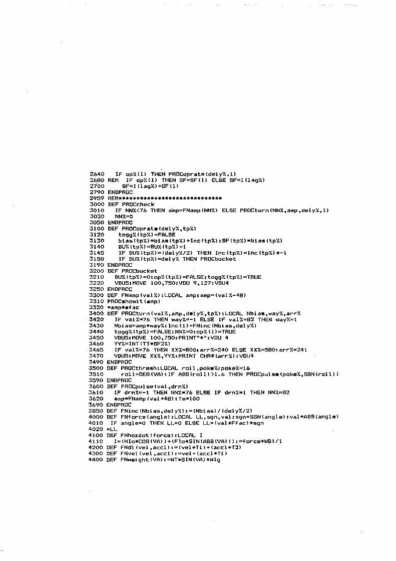
2640 2680 2700 2790 2959 3000 3010 3030 3050 3100 3120 3130 3140 3145 3150 3190 3200 3210 3220 3250 3300 3310 3320 3400 3420 3430 3440 3450 3460 3465 3470 3490 3500 3510 3590 3600 3610 3620 3690 3850 4000 4010 4020 4100 4110 4200 4300 4400
IF op%(l) THEN PROCoprate(dely%~l) REM IF cp'l.(l) THEN SF=SF(I) ELSE SF=I(lag'l.)
SF=I(lagX)+5F(1) ENDPROC REM***************************** DEF PROCcheck
IF NN'X<76 THEN a·mp=FNarnpCNNX) ELSE PROCturnCNN1.,amp,delyX,l) NN'l.=O
ENDPROC DEF PROCcprate(delyX,tpX)
tcgg'l. (tp'l.) =FALSE biasCtpX)=biasCtpX)+IncCtpX):SFCtp'l.)=biasCtp'l.) BU'l.(tp'l.)=BU'l.(tp'l.)+1 IF BUYo(tp'l.)=(dely'l./2) THEN Inc(tp'l.)=Inc(tp'l.)*-1 IF BU'l.(tpX)=delyX THEN PROCbucket
ENDPROC DEF PROCbUcket
BU'l. (tpYo) =0: cp'l. (tp'l.) =FALSE, tcggYo (tp'l.) =TRUE VDU5:MOVE lOO,750:VDU 9,127:VDU4
ENDPROC DEF FNampCval'l.):LOCAL amp:amp=(val7.-48} PROCshowitCamp) =amp*afac DEF PROCturn(val'l.,amp,dely'l.,tp'l.):LOCAL Nbias,way'l.,arrY.
IF val'l.=76 THEN way7.=-l ELSE IF val'l.=82 THEN wayY.=l Nbias=amp*way'l.:lnc(l)=FNincCNbias,dely'l.) tcgg'l.(tp'l.) =FALSE: NN'l.=O:opYo (1)=TRUE VDU5:MOVE lOO,750:PRINT"*":VDU 4 YY'l.=INT(TT*GF2Y.) IF val%=76 THEN XXX=800Iarr%=240 ELSE XXY.=5BO;arr'l.=241 VDU5:MOVE XX7.,YV%:PRINT CHR$(arrX):VDU4
ENDPROC DEF PROCthresh;LOCAL roll,pokeX:pokeX=16
roll=DEG(VA);IF ABS(roll»1.6 THEN PROCpulse(pokeY.,SGN(roll» ENDPROC DEF PROCpulse(val,drnY.)
IF drnY.=-1 THEN NNYo=76 ELSE IF drnX~1 THEN NNX=82 amp=FNamp(val+4S):Tm=100
ENDPROC DEF FNinc(Nbias,delyY.):=(Nbias)/{delyY./2) DEF FNforce(angle):LOCAL LL,sgn,val:sgn=5GN(angle):val=ABS(angle)
IF angle=O THEN LL=O ELSE LL=tval*Ffac)*sgn =LL DEF FNhozdot(force):LOCAL I
I=(Hlo*CDS(VA»+(Flo*SIN(ABS(VA»):=force*WB1/1 DEF FNdl (vel ,accl):=(vel*Ti)+(accl*T2) DEF FNvel (vel,accl):=vel+(accl*Tl) DEF FNweight(VA):=WT*SIN(VA>*Wlg

4500 4600 46io 4700 4800 4900 4999 6000 6020 6030 6035 6060 6070 6080 6090 6100 6120 6125 6130 6135 6140 6190 6200 6999 7500 7510 7515 7520 7530 7590 7999 8500 8520 8590 8600 8700 8710 8720
DEF FNpetal(VA,FF):=FF*COS(ABS(VA»*FIg*-l DEF FNfwdct(5F)
=«SF*bar»/Fwlo DEF FNturni(force):=ATN«force*Ti)/MOM) DEF FNhcirc(angle):=angle*WBl DEF FNturnw(angle)~=angle/Ti REM************************************** DEF PROCrun:LQCAL HwDOT,VwDOT,Sdot,RAi,HAi,VAi,SAi,Roti,VSDOT,SSdot
Fl=FNforce(OEG(Ll»:F2=FNforce(DEG(L2»:FF=Fl+F2 HwDOT=FNhozdot(Fl-F2):VwDOT=FNweight(VA)+FNpatal(VA,FF) Sdot=FNfwdot(SF) RAi=FNturni (FF):HAi=FNdl (Hw,HwDOT):VAi=FNdl (Vw,VwDOT):SAi=FNdl (Sw,Sdot) RA=RA+RAi1HA=HA+HAi:VA=VA+VAi:SA~SA+SAi
Roti=(FNhcirc(HAi)/Sj):L2=HA-(RA-Roti):L!=SA-(RA+Roti) Rw=FNturnw(RAi):Hw=FNvel (Hw,HwDOT);Vw=FNvel (Vw,VwDOT): Sw=FNvel{Sw,Sdot) TT=TT+Ti:REMTrl=FNtrail(RSA,VA) B4=B3.B3=B2.B2=Bl.Bl=VwDOT C6=C5.C5=C4.C4=C3.C3=C2.C2=Cl.Cl=5dct VSDOT= (Bl+B2+B3+B4)/4: PROCcontrol (VwOOT,Vw) SSdot=(Cl+C2+C3+C4)/4 R5A=5A-HA,5PV1=VwDOT.5PV2=V5DOT.5PV3=5dct PROCdraft{OEB(VA) ,DEB(RSA),DEB(VSDOT) ,DEB(5Sdot),DEG(Vw) ,TT)
ENDPROC REM******************* DEF PROCdra4t(D(1),D(2),D(3),D(4),O(S),TT):LOCAL XX%,VY%:YV%=INT(TT*GF2'l.)
FOR M=l TO 5 XX'l.=(CH(M,l)-(D(M)*F(M») MOVE CH(M,2),CH(M,3):DRAW XXX,VV1.:CH(M,2)=XXX:CH(M,3)=YVX:NEXT IF INT(TT»T5 THEN VDU 5.MOVE O,VV'l..PRINT INT(TT).VDU 4.TS=TT
ENDPROC REM************************* DEF PROCtitle PRINT;TAB (3) ; OT:$; "Speed= "FNmph (VV'l.)" mph . Sl "51" 52 "92 ENDPROC DEF FNmph(fps)1=(fps/SB)*60 DEF PROCshowit(val)
VOU5:MOVE lOO,BOO:VDU 9,9,127,127:PRINT val:VDU4 ENDPROC

10 REM************************************* 20 REM FINDING MOMENTS OF INERTIA ~O REM************************************* 50 NN=26.N2=5.DIM NM$(NN).DIM NB(NN).DIM DM$(NN).DIM DT$(NZ).DIM DT(N2) 90 @X=&20309:satis=0:DT$=II"
100 WB=O: Wradl=O: Wrad2=0: bi' kea=O:bi keb=O:rake=O' trl=OI Bmas=O: FWma9=O 110 Sgravl=0IBgrav3=0~Sgrav2=0=Bgrav4=0:Mht=0:Mrad=0:Mma9=O:Mgravl=O 120 Mgrav3=0: Mgrav2=O:Mgrav4=0: mass=O:WT=O:HG=O,LG-O:bar=O :barmas=O 136 Fwfac=I.4144:REM Convert to solid disc equivalent 150 WIo=O:REM Vert moments about Ground contact point 160 Flo=O:REM Vert moments about C of G 170 Hlo=O:REM Hoz moments about C of G 180 Llo=O:REM Hoz moments about rear wheel 190 g=32:REM Gravity 199 REM********************************************* 200 REM Main 210 CLS 220 PROCnames:PROCnumbs_in:PROCallocate 600 PROCmoments:DT(5)=FNfwheel(Wradl,Fwfac,FWmas,bar,barmas):REM Fwlo 800 PROCfinal:PROCshow:IF satis THEN PROCfile 900 MODE 3.END 999 REM********************************************:::
1000 DEF PROCmoments 1010 LOCAL Hmom,Bmom 1040 REM Vert ----------------------1050 Mmom=Hmas*«{Mrad~2)/4)+«Mht~2)/12»:Bmom=Bmas*Cbikea~2)/12 1055 REM about road contact pt. 1070 DT(I)=FNmoms(Mgravl,Bgravl):REM Wlo 1080 REM Vert about CG 1090 DT(2)=FNmomsCMgrav2,Bgrav2):REM FIe 1100 REM Hoz -----------------------1110 Mmom=Mmas*CMrad~2)/2:Bmom=Bma5*(bikeb~2)/12 1115 REM about CB 1120 DT(3)=FNmomsCMgrav4,Bgrav4):REM HIe 1125 REM about rear wheel 1130 DT(4)=FNmoms(Mgrav3,Bgrav3):REM LIo 1140 ENDPROC 1150 DEF FNmomsCman,bike):=(Mmom+(Mmas*(manA 2»)+CBmom+(Bmas*(bikeA 2») 1200 DEF FNfwheel(rad,fac,Wmas,bar,barmas):LOCAL Qrad,Wmom,Bmom 1210 Bmom=barmas*Cbar~2)/12 1220 Qrad=rad*fac:Wmom=(Wmas*(Qrad~2)/4)
1230 =Wmom+Bmom 2000 DEF PROCnames 2010 DATA "Wheel Base" ,"Front Wheel RadII, "Rear Wheel Rad tl , "Effect. Ht" 2020 DATA "Effect. Lgth", "rake", tltrl" ,IIBi ke mass", "FWmass", "Bgravl", "Bgrav3", tls
grav2", "Bgrav4" 2030 DATA "Man Ht", "Man Rad", "Man Mass", "Mgrav1", "Mgrav3", "Mgrav2", "Hgrav4" 2040 DATA "Comb Mass", "Comb WT", "Comb Grav Ht", "Comb Grav Lgth 11 ,"Bar eff. I ngth"
1 "Bar mass" 2050 DATA "ft", "ft" I "ft", "ft", "ft·" "degs", "ft", "slugs", "slugs", "ft", "ft", "ft"
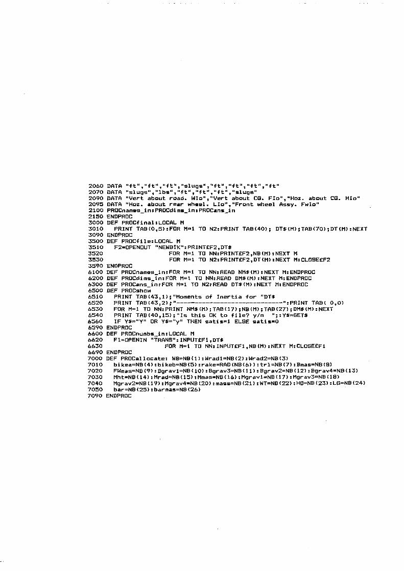
2060 2070 2090 2095 2100 2150 3000 3010 3090 3500 3510 3520 3530 3590 6100 6200 6300 6500 6510 6520 6530 6540 6560 6590 6600 6620 6630 6690 7000 7010 7020 7030 7040 7050 7090
DATA "ft", "ft", "ft", "slugs", "ft", "ft" I "ft", "ft" DATA "slugs","lbs","ftll,"ft","ftll,"slugs" DATA "Vert about rDada WIo", "Vert abDut CG. FIe", "Hoz. about CB. HIe" DATA "Hoz.. about rear wheel. LIo", "Front wheel Assy. Fwlo" PROCnames_in:PROCdims_in:PROCans_in ENDPRDC DEF PROCflnal'LOCAL M
PRINT TAB(0.5).FOR M=1 TO N2.PRINT TAB(40); DT$(M);TAB(70);DT(M).NEXT ENDPROC DEF PROCfl1e.LDCAL M
F2=OPENDUT "NEWBIK".PRINT£F2.DT$ FOR M=1 TO NN.PRINT£F2.NB(M).NEXT M FOR M=1 TO N2.PRINT£F2.DT(M).NEXT M.CLOSE£F2
ENDPROC DEF PROCnames_in:FOR M=l TO NN:READ NM$(M):NEXT M:ENDPROC DEF PROCdims_in.FOR M=l TO NN.READ DM$(M).NEXT M.ENDPROC DEF PROCans_in:FOR H=l TO N2:READ DT$(M):NEXT M:ENDPRQC OEF PROCshow
PRINT TAB (43,1) ; "Moments of Inerti a for "DT$ PRINT TAB(43,2);"----------------------------":PRINT TABe 0,0) FOR M=1 TO NN:PRINT NM$(M);TAB(17);NB(M);TAB(27);DM$(M).NEXT PRINT TAB(40,15);"ls this OK to file? y/n II p YS=GET$ IF Y$="Y" OR V$="y" THEN satis=l ELSE satis=O
ENDPROC DEF PRDCnumbs_in:LOCAL M
Fl=OPENIN "TRANS".INPUT£Fl.DH FOR M=1 TO NN:INPUT£Fl.NB(M).NEXT M.CLOSE£Fl
ENDPROC DEF PRDCallocate: WB=N8(1):Wradl=NBC2):Wrad2=NB{3)
bikea=NB(4):bikeb=NB(5):rake=RADCNB(6»:trl=NB(7):Bmas=NBCS) FWmas=NB(9):Bgravl=NB(10):Bgrav3=N8(11):Bgrav2=NBC12):Bgrav4=NB(13) Hht=NB(14):Hrad=N8(15):Hmas=NB(16):Hgravl=NBC17):Mgrav3=NB(18) Mgrav2=NB(19):Hgrav4=NB(20):mass=NB(21):WT=NB(22):HG=NB(23):LG=NB(24) bar=NB(25):barmas=NB(26)
ENDPROC

--o
--- ---- --- --- --- ----- -- -- +-+ ----+ _--++~-----3
, \ \
-....... --~ ............. (")
----- ,,.. (,Q ............. \,1I0oI

~I , 'f." f~,,\AY . .l
'.'
E ent
I 11 1111111111 I 1111 I11 11 I 11 I 11 11 11 I t 11 I 11111 I I 11 1111 I11 11 11 1111 I11 I11 111111 I
188 288 388 488 588 688 788
Run 25. Roll and Ba~ angles
E ent
I i I11 i i i I i I i i 11111 i 11 i 111111111111 i 11111111 i I i I ill i 1111111111111111111 i i 11 i
188 288 308 488 588 688 788
Run 26. Roll and Ba~ angles

. .,.., ~'-'.' ~I~
E ent
? ?
""""'1""""'1""""'1""""'1""""'1""""'1""""'1"'" 180 288 300 400 500 600 780
Run 27. Roll and Bar angles
(.1 I, I ... 1 11;,;.i1't _.~r 9 ....... ;:J ...... ,
'u' .'} 1:::....1 ............. ,1 ....
'-,
E ent
I, , , , , 11 , 'I' ill' 11 , 'I' , , , , , , , , ! ' , , , , , , , 'I' , , , , , , iI i ' , 11 , , , , i 1"11 , 1 i , 1 111 , , 1
180 288 388 408 588 608 708
Run 28. Roll and Bar angles

E ent
11111111111111111111111111111111111111111111111111111111111111111111 1111111
100 200 388 488 588 688 788
Run 29. Roll and Bar angles
\.--~:..[
E ent
1111111111111 i I i 1111111111 i 111111111 i I i i 11 i I11 i 11 i I11 I11 Ill! 111111111 i 11111
188 288 388 488 500 6eS 7S0
Run 30. Roll and Bar angles

E ent
1111111111111111111111111111111111 1111111 1111 I Ill! 1111111111111111111111111
~ee 2ee 3ee 4ee see 6e0 700
Run 31. Roll and Bar angles
Efent
I11111111 i j I i i i 111111111 i i i 11 i 111111 i I i 11 i i i i i i i I i 111111 i I i i j i 11111 i 1111 i i 11
I ~0e 200 300 400 509 699 790
Run 32. Roll and Bar angles

E en-t
? ?
111111111111111111111111111 111111111111 111111111111111111111111111111111111
100 200 300 400 500 600 700
·Run 33·, Roll and Bar angles
..... I!') !-.
I'I:~} \'. 1t.!{J~ '.
E ent
1'1 j IIIII i 11 i i I i 1\ i i I i i i i 11 i III1 '111.11 i Illllill i I i i I' i 111\ i i '1111111111111 i I i
I 10a 209 3a0 4a0 500 6a8 708
Run 34. Roll and Bar angles

- A l·~ .J't.... - ,."j'l.J c. .' I '<-.. ,.,.,. .'1'/ L I ,'): till f I I'
. '':.no ,/"'-')',,.. I 1 •. :;. ........ ;rh I I ~d.~'~ 11 ~ ! IIL..-----+f--' I ~. i ~ _.t ~ ~ .... I I,. j r'l J .. I 1.1... I' I, l ......... ,_ ", -. ,--,' -"'''''''-', ,I' Id} t .. /,' ---..O"\;f .... .....,. ~ .~ .. I".,l' \Lr~l
I,' '- ......., r,l ~ ..... .I·L'11 ' ... '..... ~-.......J. '.1
E ent
111111111111111111111111111111111111111111111111111111111111111111111111111
109 209 308 408 500 600 700
Run 35. Roll and Ba~ angles
E ent
11111111111111111111111111111111111111111111111111111111111111111111 1111111
188 208 388 488 588 688 788
Run 36. Roll and Ba~ angles

Run Ho 25 Roll and 8ar (dal'k line) 8n91e ?
1 1 1 1 1 1 1 1 1 I 1 1 1 1 1 1 1 1 1 I 1 1 1 -I 1 1 1 1 1 I 1 1 1 1 1 1 1 1 1 I 288 389 498 588
Run Ho 25 Roll and 8ar (dark line> Velooity
1 1 1 1 1 1 1 1 1 I 1 1 1 1 1 1 1 1 1 I 1 1 1 1 1 1 1 1 1 I 1 1 1 1 1 1 1 1 1 I 288 388 488 588
Run Ho 25 Roll and Oar (dark line) 800ln ?
1 1 1 1 1 1 1 1 1 I 1 1 1 1 1 1 1 1 1 I 1 1 1 1 1 1 1 1 1 I 1 1 1 1 1 1 1 1 1 I 288 388 488 588
Run Ho 25 Roll and Bar (dark line) Jerk ?
11 1 1 1 1 1 1 1 1 I 1 1 1 1 1 1 1 1 I 1 1 1 1 1 1- 1 1 1 I 1 1 1 1 1 1 1 1 1 I 218 388 481 511

? Run Ho 26 Roll and Bar (dark lin.) Angle
I I I I I I I I I I I I I I I I I I I I I I I I I I I I I I I I I I I I I I I I 218 al8 41. 58.
? Run Ho 26 Roll and Oar (dark line) Velooity
I I I I I I I I I I I I I I I I I I I I I I I I I I I I I I I I I I I I I I I I 2B8 a88 4BB 58.
Run Ho 26 Roll and Oar (dark line) ftccln ?
I I I I I I I I I I I I I I I I I I I I I I I I I I I I I I I I I I I I I I I I 2BB a88 48B 5BB
Run Ho 26 Roll and Oar (dark line) Jerk ?
I I I I I I I I I I I I I I I I I I I I I I I I I I I I I I I I I I I I I I I 2BB 388 488 588

Run Ho 27 Roll and Bar (dark lino> nnglo
I I I I I I I I I I I I I I I I I I I I I I I I I I I I I I I I I I I I I I I I 288 388 488 588
Run Ho 27 Roll and Bar (dark lino> Uoloeity
I I I I I I I I I I I I I I I I I I I I I I I I I I I I I I I I I I I I I I I I 288 388 488 588
Run Ho 27 Roll and Bar (dark lino> Reeln
I I I I I I I I I I I I I I I I I I I I I I I I I I I I I I I I I I I I I I I 288 398 488 588
Run Ho 27 Roll and Bar (dark lino> lerk
I I I I I I I I I I I I I I I I I I I I I I I I I I I I I I I I I I 288 398 488 588

? Run Ho 28 Roll and Bar (dark line) Angle
I I I I I I I I I I I I I I I I I I I I I I I I I I I I I I I I I I I I I I I I 288 388 488 588
? Run Ho 28 Roll and Bar (dark line) Uelocity
I I I I I I I I I I I I I I I I I I I I I I I I I I I I I I I I I I I I I I I I 289 388 489 588
Run Ho 28 Roll and Bar (dark line) Accln ?
I I I I I I I I I I I I I I I I I I I I I I I I I I I I I I I I I I I I I I I I 28B 388 488 588
Run Ho 28 Roll and Bar (dark line) Jerk ?
i I I I I I I I I I I I I I I I I I I I I I I I I 288 388 488 588

? Run Ho 29 Roll and Bar (dark line> Angle
I I I I I I I I I I I I I I I I I I I I I I I I I I I I I I I I I I I I I I I I 288 388 488 588
? Run Ho 29 Roll and Bar (dark line> Uelocity
I I I I I I I I I I I I I I I I I I I I I I I I I I I I I I I I I I I I I I I I 288 388 488 588
Run Ho 29 Roll and Bar (dark line> Rccln ?
I I I I I I I I I I I I I I I I I I I I I I I I I I I I I I I I I I I I I I I I 288 388 488 588
Run Ho 29 Roll and Bar (dark line> 1erk ?
I I I I I I I I I I I I I I I I I I I I I I I I I I I I I I I I I I I I I I I I 288 388 488 588

· - -.', .. , ~- ..
Run Ho 31 Roll and Bar (dark lin~) Hngl~
I I I I I I I I I I I I I I I I I I I I I I I I I I I I I I I I I I I I I I I I 21. 3.1 4.1 511
Run Ho 3. Roll and Bar (dark line) Uelocity
I I I I I I I I I I I I I I I I I I I I I I I I I I I I I I I I I I I I I I I I 2.1 31. 41. 511
Run Ho 38 Roll and Bar (dark line) Hccln ?
I I I I I I I I I I I I I I I I I I I I I I I I I I I I I I I I I I I I I I I I 288 381 488 588
Run Ho 3. Roll and Bar (dark line) Jerk ?
I I I I I I I I I I I I I I I I I I I I I I I I I I I I I I I I I I I I I I I I 211 388 488 588

Run Ho 31 Roll and Bar (dark line> flngle
I I I I I I I I I I I I I I I I I I I I I I I I I I I I I I I I I I I I I I I I 288 388 488
Run Mo 31 Roll and Bar (dark line> Velocity
I I I I I I I I I I I I I I I I I I I I I I I I I I I I I I I I I I I I I I I I 288 388 488 588
Run Ho 31 Roll and Bar (dark line> flccln
v
I I I I I I I I I I I I I I I I I I I I I I I I I I I I I I I I I I I I I I I I 288 388 488 588
Run Ho 31 Roll and Bar (dark line> Jerk
I I I I I I I I I I I I I I I I I I I I I I I I I I I I I I I I I I I I I I I I 2B8 388 488 588

Run Ho 32 Roll and Oar (dark line> Rngle 1
I I I I I I I I I I I I I I I I I I I I I I I I I I I I I I I I I I I I I I I I 288 398 488 588
Run Ho 32 Roll and Oar (dark line> Ueloeity
I I I I I I I I I I I I I I I I I I I I I I I I I I I I I I I I I I I I I I I I 288 388 488 588
Run Ho 32 Roll and Oar (dark line> Reeln
R •
~~~#J!~ I I I I I I I I I I I I I I I I I I I I I I I I I I I I I I I I I I I I I I I I
289 388 488 588
Run Ho 32 Roll and Bar (dark line> Jerk
I I I I I I I I I I I I I I I I I I I I I I I I
289 388 488 588

, ',._'. . '- ,.'-.
?
?
?
?
- .. '~ ~'- .
Run Ho 33 Roll and Oar (dark linp) 8ng\p
I I I I I I I I I I I I I I I I I I I I I I I I I I I I I
288 388 488
Run Ho 33 Roll and Oar (dark line) Velocity
1111111111
588
I I I I I I I I I I I I I I I I I I I I I I I I I I I I I I I I I I I I I I I I 288 388 488 588
Run Ho 33 Roll and Oar (dark line) Rccln
I I I I I I I I I I I I I I I I I I I I I I I I I I I I I I 288 388 488
Run Ho 33 Roll and Oar (dark line) Jprk
111111111
588
I I I I I I I I I I I I I I I I I I I I I I I I I I I I I· I I I I I I I I I I 288 388 488 588

Run Ho 34 Roll and Oar (dark lin!) Rngl! ?
I I I I I I I I I I I I I I I I I I I I I I I I I I I I I I I I I I I I I I I I 211 388 418 588
? Run Ho 34 Roll and Bar (dark line) Ueloeity
I I I I I I I I I I I I I I I I I I I I I I I I I I I I I I I I I I I I I I I I 288 388 488 588
Run Ho 34 Roll and Bar (dark line) Reeln ?
I I I I I I I I I I I I I I I I I I I I I I I I I I I I I I I I I I I I I I I I 288 389 488 588
Run Ho 34 Roll and Oar (dark line) Jerk
I I I I I I I I I r I I I I I I I I I I I I I I I I I I I I I I I I I I 288 388 488 588

? Run Ho 35 Roll and Oar (dark line) Rngle
I I I I I I I I I I I I I I I I I I I I I I I I I I I I I I I I I I I I I I I I 288 388 488 588
1 Run Ho 35 Roll and Oar (dark line) Velocity
I I I I I I I I I I I I I I I I I I I I I I I I I I I I I I I I I I I I I I I I 288 388 488 588
Run Ho 35 Roll and Oar (dark line) Rccln 1
I I I I I I I I I I I I I I I I I I I I I I I I I I I I I I I I I I I I I I I I 288 388 488 588
Run Ho 35 Roll and Oar (dark line) Jerk ?
I I I I I I I I I I I I I I I I I I I I I I I I I I I I I I I I I I I I I
288 388 488 588
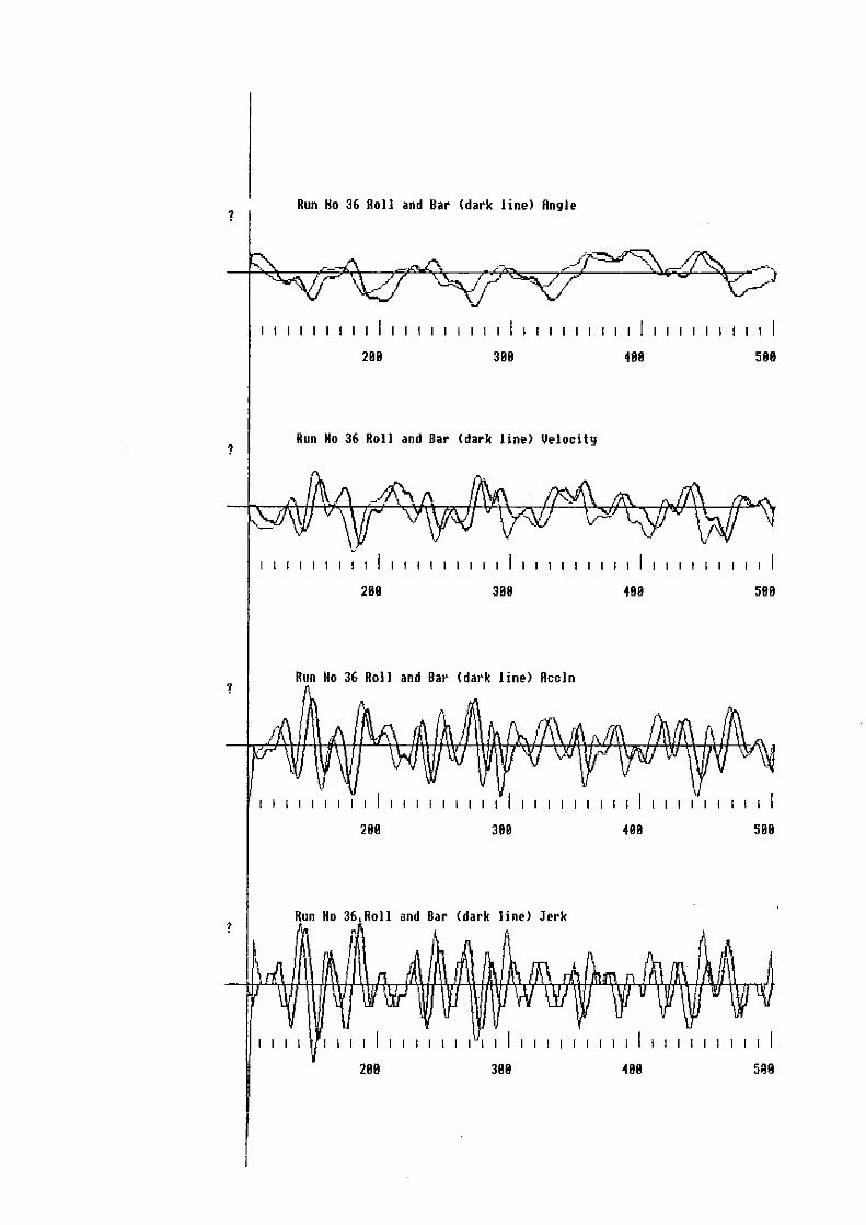
? Run Ho 36 8011 and Oar (dark line) 8ngle
I I I I I I I I I I I I I I I I I I I I I I I I I I I I I I I I I I I I I I I I 288 388 488 588
Run Ho 36 Roll and Bar (dark line) Velocity
I I I I I I I I I I I I I I I I I I I I I I I I I I I I I I I I I I I I I I I 288 388 488 588
Run Ho 36 8011 and Ba,' (da,'k line) Rccln
288 388 488 588
and Bar (dark line) Jerk ?
f I
I
l J I I I I I I I I I I I I I I I I I I I 1111111 I I I I I I I I I I I I I
288 388 488 5~8

t1DRARA all runs
Mid-pt Freq
5 13 ************* 15 10 ********** 25 20 ******************** 35 16 **************** 45 18 ****************** 55 14 ************** 65 20 ******************** 75 10 ********** 85 18 ****************** 95 13 ************* 105 16 **************** 115 12 ************ , 125 8 ******** 135 9 ********* 145 10 ********** 155 14 ************** 165 9 ********* 175 6 ****** 185 6 ****** 195 9 *********
* (1) Mean = 114.114094
MDBARA all runs
Mid-pt Freq
5 17 15 13 25 24 35 17 45 18 55 15 65 16 75 17 85 18 95 24 105 9 115 13 125 18 135 6 145 11 155 8 165 8 175 10 185 3 195 0
* Cl)
***************** ************* ************************ ***************** ****************** *************** ***********'***** ***************** ****************** ************************ ********* ************* ****************** ****** *********** ******** ******** ********** ***
Mean 100.422819
Std. Dev.= 83.7320775
Std. Dev.= 81.6115518

ADRARA all runs
Mid-pt Freq
5 19 15 12 25 5 35 14 45 12 55 8 65 12 75 7 85 11 95 12 105 12 115 8 125 15 135 12 145 6 155 7 165 9 175 7 185 7 195 7
* (1)
******************* ************ ***** ************** ************ ******** ************ ******* *********** ************ ************ ******** *************** ************ ****** ******* ********* ******* ******* *******
Mean 115.298755 Std_ Dev.= 79_2304923
ADBARA all runs
Mid-pt Freq
5 28 15 16 25 5 35 8 45 9 55 12 65 12 75 14 85 12 95 11 105 5 115 7 125 15 135 7 145 7 155 3 165 5 175 7 185 8 195 10
* = (1)
**************************** **************** ***** ******** ********* ************ ************ ************** ************ *********** ***** ******* *************** ******* *******
*** ***** ******* ******** **********
Mean 116.091286 std. Dev.= 104_80264

f'1DRWAV all runs
Mid-pt Freq
1 0 3 5 5 13 7 46 9 68 11 61 13 33 15 21 17 15 19 14 21 8 23 8 25 2 27 2 29 2 31 0 33 0 35 0 37 0 39 0
* (2)
** ****** *********************** ********************************** ****************************** **************** ********** ******* ******* **** ****
* * *
Mean 11.2013423 Std. Dev.= 4.83760419
MDBl-'JAV all runs
Mid-pt Freq
1 3 3 5 5 10 7 48 9 85 11 58 13 33 15 23 17 11 19 6 21 6 23 3 25 2 27 4 29 1 31 0 33 0 35 0 37 0 39 0
* (2)
* ** ***** ************************ ****************************************** ***************************** **************** *********** ***** *** *** * * ** ..
Mean 10.4261745 Std. Dev.= 4.52690534

ADRl'JAV all runs
Mid-pt Freq
1 3 5 7 9 11 13 15 17 19 21 23 25 27 29 31 33 35 37 39
o 2 14 16 21 29 44 30 33 24 6 6 6 2 3 4 1 o o o
( I )
ADBWAV all runs
Mid-pt Freq
I 4 3 8 5 21 7 20 9 26 11 35 13 41 15 29 17 15 19 19 21 12 23 6 25 4 27 0 29 0 31 1 33 0 35 0 37 0 39 0
* (1)
** ************** **************** ********************* ***************************** ******************************************** ****************************** ********************************* ************************ ****** ****** ******
** *** **** *
Mean 13.8381743 Std. Dev.= 5.72201427
**** ******** ********************* ******************** ************************** *********************************** ***************************************** ***************************** *************** ******************* ************ ****** ****
Mean 11.9917012 Std. Dev.= 5.47570394

ADU::'G all runs
Mid-pt Freq
0 0 1 28 2 27 3 49 4 43 5 37 6 16 7 18 8 12 9 6 10 2 11 1 12 2 13 0 14 0 15 0 16 0 17 0 18 0 19 0
" = (2)
************** ************* ************************ ********************* ****************** ******** ********* ******
*"" * .. *
Mean 4.2033195 Std. Dev.= 2.28020286
MDLAG all runs
Mid-pt Freq
0 0 1 19 2 75 3 88 4 62 5 35 6 7 7 1 8 4 9 4 10 2 11 1 12 0 13 0 14 0 15 0 16 0 17 0 18 0 19 0
" (2)
********* ************************************* ******************************************** ******************************* ***************** .... * " ** "* * ..
Mean 3.36912752 std. Dev.= 1.63579504

5 \ 1
4 I \
3
\ 2
.1. \ \
\
..... ph Gain S
90 Lag .1.2
( 5) (.1.0) (.1.0)
\ ) \\ /
... r/O ./
( ( ---
I
I
./
("

BIKE C 4 Mph Gain 288 Lag 12 Secs R S R~~ S~~
( 2) ( 2) (18) (15)
? ( ,(
5 --" ;,) )
4 ( ( < ) ->
(~~~ ( ( 3 ---.
-) ~.
,------ ----~
2 ( ) c:- ------- ---• --~
'i" ---") _____ ... 1
--- --(
---\ <~~- '-
( -----
1 f-~~-::::;, _---
------., -
\ --- c-----1-----
<. -----
R~
5) (
)
( }
(
D (
t'l , (

BIKE C 4 Secs R
( 2)
5
4
3
2
1
l\
..... ph
S (
"'-, ./
C) ('
) (
)
:> '" ..... , ..
Gain 228 Lag 12 S~~
2) (25)
--
<--=-~-=~ r-------- ( (.:----
~~~~~::;, ) --- -------::. ~-- ---- ( ·C: (:----r---... ) ~-==--~-, ,------ '-----;>
r----- ------ ( "-----
1------;. --=--=-.-=.-".) )
---- --- r;:----- ( .:: -----~--1------ -----....
.. , __ ---..I " )
( ,------r------ [:=~=~ ------
I---~ -----) 1'-, .) -----
...
,---- 1---- (----- ( --

3
2
J_
/"
~ ')
( \
Mph Gain 248 Lag 12 S R........ S ........ R~
( 2) (28) (55) ( 5)
---- 1-- ---:::~.> _.:=:-:.. ---1----- 1;---
<-::-=-_ , ------1--r--_ _-:.-::--"".::. ~,
----1-----r';:------
-~~~:~ (" ---
(-- (

Run 25 Residuals >1.96 std. dev ?
?
I I I I " I 11 I I I
280
I I I I I "l" 300
I I I I I "l" .400
Run 26 Residuals >1.96 std. dev ?
?
I I I I I I I "1" 280
11 I I I "1" 300
I I 11 I I
11
I I I I
488
I I I I I I I I 501
.. ,-.-
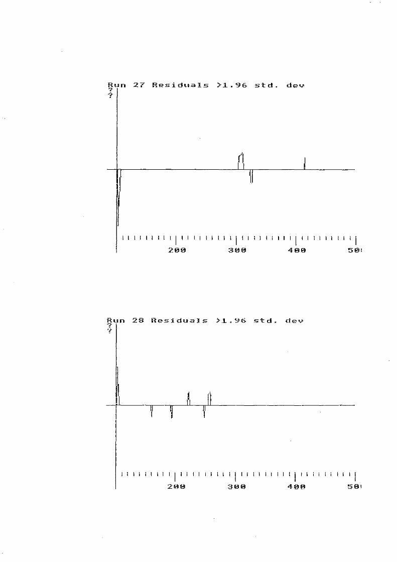
Run 27 Residuals >1.96 std. dev ?
1-
·'1
H 11
I I I I I I I I I I 11 11 I I
290
I I I I I I I I I I I I I I I I 409 '501
Run 28 Residuals >1.96 std. deu ?
1-
I
\ j (I -1' ~ ~ it
'I' ,
I I i I i 1 I I i i I , 400
I I I I '501

Run 29 Residuals >1.96 std. dev ~
1"
"
/
I I I I I I I I I 1 I I I I I I I 11 1 I I I I I I I
288 388
Run 38 Residuals >1.96 std. dev ~
1"
I I I I I I I I I 1 I I
288
I I I I I I I 1 I I
388
I I I I I I I 1 I I
488
I I I I I I I 1
581
11111111
581

Run 3~ Residuals >~.96 std. dev ? ?
I I 11 I I I I I I I I
288
I I I I I I I I I I
388
I I I I I I I I I I
488
Run 32 Residuals >~.96 std. dev ?
?
I I I I I I I I I I I I
288
I I I I I I I I
399
I I I I I I I I
499
I I I I I I I I 591
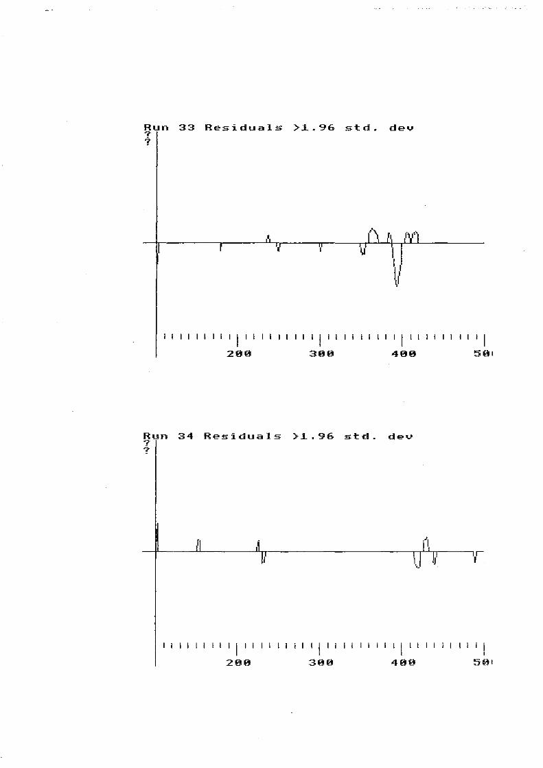
Run 33 Residuals >1.96 std. dev ?
?
" I I I I I I I I I I "l" 399
I I I I I I I I " 499
I I I I I I I I 591
Run 34 Residuals >1.96 std. dev '~
1"
I I I I I I I "l" 299
I I i I I I
390
I I I
\,1 Il "
I I " " 499

Run 35 Residu~ls >1.96 std. deu ? 1-
1 1 1 1 1 1 1 1 1 I 1 i
288
1 1 1 1 1 1 1 I 1 1
388
IJ
1 1 1 1 1 1 1 I 1 1
488
Run 36 Residuals >1.96 std. deu ?
1-
i 1
1 1 1 1 1 1 1 I 581
~u-~------nr---·-----~~------------------·--,,-----'ll
1 1 1 1 1 1 1
IJ
"1" 280
1 1 1 1 1 1 1 i ill 1 1 I
388
11 1 I Ii 488

Run 25 Roll angles + pushes '?
.--" .'-',
--........ -.. -........ J.--_ ... -
, , , , 11 , "I" 288
11 , " , , 11 , "1""""'1 488 581
Run 26 Roll angles + pushes ?
11111111
-._--",,-- / ... __ .....
'I'''''''' 288
, I ' , 388
111111 , I ' , 488
Run 27 Roll angles + pushes .•. ? .....
T
"""I 581
""""'1""""'1""""'1""""'1 288 388 408 581
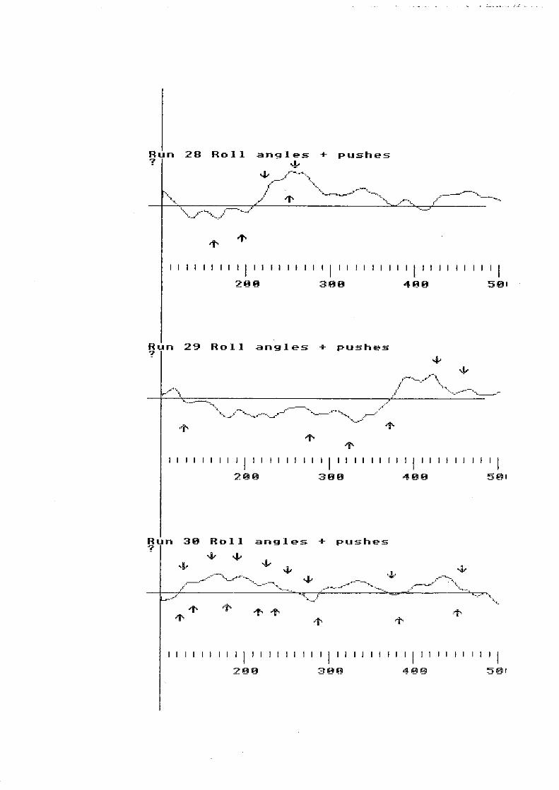
Run 28 Roll angles + pushes
? '"
.. , .......
~ . :---.. . :.,-.~
--. ----
I I 11 I I I I I I I I I I I I I 11 I 11
299 399
I I I I I I I I 11
499
I I I I I I I I 501
Run 29 Roll angles + pushes '?
.......... -. , ~ ~
.•.. ,-.. ----'" ......... ,.-...... ~--•. -....... -~-'-.--......... -- ~--......... .-. ......-... " .... _.-.
I I I I I I I I I I I I I I I I I I I I I 111111111111111111
Run ?
290 309
30 Roll angles + pushes
....... J/
400 501
,.,...-....... -. ... ---....r'" '.
, L_.-. .' . -.. ..,-
I I I I I I I I I I I I I I I I I I I I I I I I I I I I I I I I I I I I I I I I 200

Run 31 Roll angles + pushes .?
.l \ ... ,-
I I I I I I I I I I I I
288
.--............
1111111111111111
399
angles -I- pushes
I I I I
498
I I I I I I I I 58'
\_. -"'-- j
1111111111" 111111111111111111111111111
299 3!lt9 499 59.
Run 33 Roll angles + pushes ?
..J,.- "-' ,/\ -+---'~O:-----"~~"--------=="7":--=,-+} ........ "'----r::---
. .-r-.r-. --_~ ....... _, .••.. ,--........ -...~ ................ _--......_~ ..... __ ~-_.-. _0- .• ,_............ ,; ", -'! .. ~-~.--...L-.-
.... l \.l
1"-I I I I I I I I I I I I I I I I I I I I I I I I I I I I I I I I I I I I I I

Run 34 Roll angles + pushes '?
I I I I I I I I I I I I
2~Ht
111111111111111
380
¥F.35 RoU angles + pushes
r '-,. ..-., ~ " __ '.. , .. "r '_
11 I I I I I I I I I I I 400 501
I I I I I I I I I I I I I I I I I I I I I I I I I I I I I I I I I I 11 I 11 I 200 3~0 400 501
Run 36 Roll angles + pushes:
'I
_.Jl
:,.,."" ... ,. .-.~ . I'~
-'-"., .. ,.' \ ....... r.' , .... ,--_ ...
.1'
I I I I I I I I I I I I I I 11 I I I I I I I I I I I I I I I I I I I I I I I I
l