Embed Size (px)
Citation preview

2010032
M A S T E R S T H E S I S
Geometrical projectile shapeseffect on hypervelocity impact
Asra Monthienthong
Lulearing University of Technology
Master Thesis Continuation Courses Space Science and Technology
Department of Space Science Kiruna
2010032 - ISSN 1653-0187 - ISRN LTU-PB-EX--10032--SE
CRANFIELD UNIVERSITY
SCHOOL OF ENGINEERING
MSc in Astronautics and Space Engineering
MSc THESIS
Academic Year 2008-2009
Asra Monthienthong
Geometrical Projectile Shapes Effect on Hypervelocity Impact
Supervisor R Vignjevic
June 2009
This thesis is submitted in partial fulfilment of the requirements
for the degree of Master of Science
copy Cranfield University 2009 All rights reserved No part of this publication
may be reproduced without the written permission of the copyright owner
Asra Monthienthong
i
Abstract
All spacecraft confronts threat of space debris and meteoroids Spherical projectiles are
common shape used to study impact of space debris on spacecraft structures or shielding
system However real space debris which is a threat to spacecraft is not likely to be
spherical There is a need to study the influence of projectile shape as non-spherical
shapes may cause greater damage to spacecraft than spherical projectiles with same
impact conditions
The aim of this research is to investigate the effect of projectile shapes focusing on
impact velocity in hypervelocity range by numerical simulations The geometrical
shapes of projectiles that were simulated are sphere cylinder and cube Projectiles and
targets are made of aluminium 2024 All projectiles have equivalent mass hence
equivalent impact energy The impact velocities are 3 kms 5 kms 7 kms and 9 kms
Smoothed particle hydrodynamics (SPH) is applied
The shapes of debris clouds velocities of debris clouds residual velocity of projectiles
dimension of target hole after impact impact induced stress and target failure modes are
investigated and compared between different projectile shapes Shapes of debris clouds
generated by impact of cylindrical and cubic projectiles have spike-like in frontal area of
the debris clouds which do not exist in that of spherical projectile Velocities of debris
clouds generated by the impacts of cylindrical and cubic projectiles are higher than that
of spherical projectile in hypervelocity impact range ie higher than 5 kms
The conventional spherical projectile is not the most dangerous case of space debris
With equivalent mass a cylindrical projectile with length-to-diameter ratio equal to 1 is
more lethal than a spherical projectile A cubic projectile is more lethal than a spherical
projectile and cylindrical projectile with length-to-diameter ratio equal to 1 and with an
equivalent mass
Asra Monthienthong
ii
Acknowledgements
I would like to thank Prof Rade Vignjevic for his advices recommendations guidance
and supervising me through this work
I would also like to thank Dr James Campbell who always gives me suggestions and has
been very helpful and to Mr Nenad Djordjevic and Dr Kevin Hughes
Thanks to Dr Jennifer Kingston and Dr Peter Roberts
Thanks especially to my beloved parents sister and brother who always support me in
every step I take and everywhere I am
Asra Monthienthong
iii
Contents
Abstract i
Acknowledgements ii
Contents iii
List of Figures v
List of Tables viii
Nomenclature ix
Abbreviations x
1 Introduction 1
11 Space Debris Threat 1
12 Spacecraft Shielding System 1
13 Effect of Space Debris Shapes 2
14 Research Objectives 3
15 Research Methodologies 4
16 Research Outline 5
2 Orbital Space Debris and Protection 6
21 Introduction to Orbital Space Debris 6
22 Study in Space Debris 8
221 Space Debris Measurement 8
222 Space Debris Modelling and Risk Assessment 9
223 Space Debris Mitigation 10
23 Characteristic Length of Space Debris 11
24 Spacecraft Shielding System 11
241 Shielding System Development 11
242 Ballistic Limit Curves 13
25 Debris Cloud Characteristics 14
3 Impact Phenomena 16
31 Classification of Impact Phenomena 16
32 Impact Physics 16
321 Stress Wave 17
322 Impact Induced Stress 19
323 Shock wave 21
33 Hypervelocity Impact 24
34 Target Failure Mode 26
4 Smoothed Particle Hydrodynamics Method 28
41 Introduction to SPH and Numerical Simulation 28
42 Spatial Discretization 29
423 Alternative Method 31
43 Artificial Viscousity 31
44 SPH Formularisation 32
Asra Monthienthong
iv
421 Conservation equations 33
422 Kernel Function 36
423 Smoothing Length 37
45 Implementation in MCM 38
5 Simulation Validation 41
51 Validation and Resources 41
52 Validation of Spherical Projectile 41
521 Model Configurations 42
522 Comparisons between experiments and simulations 42
53 Validation of Cylindrical Projectile 44
6 Geometrical Projectile Shapes Impact Simulation 46
61 Model description 46
62 Measured parameters 47
621 Debris Cloud Shapes 47
622 Debris Cloud Velocities 47
623 Selected Nodal Velocities 47
624 Stress waves 48
625 Target failure 48
63 Spherical Projectile Impact 48
64 Cylindrical Projectile Impact 53
65 Cubic Projectile Impact 57
7 Comparisons of Geometrical Projectile Shapes Impact 62
71 Debris Cloud Shapes 62
72 Debris Cloud Velocities 63
73 Dimension of target hole 65
74 Induced Stress 66
8 Conclusion 68
81 Geometrical projectile shapes effect 68
82 Future work 69
9 References 70
Appendix A MCM codes 78
Asra Monthienthong
v
List of Figures
Figure 21 Trackable objects in orbit around the Earth (ESA 2008) 6
Figure 22 Spatial density of space debris by altitude according to ESA MASTER-
2001(Michael Oswald 2004) 7
Figure 23 Growth of space debris population model (ESA2008) 8
Figure 24 Space debris sizes and protection methods 10
Figure 25 Whipple bumper shield after impact of projectile and rear wall of a Whipple
shield impacted fragmentation of projectile and bumper (Hyde HITF2009)
12
Figure 26 Stuffed Whipple shield after impact of a projectile and mesh double bumper
shield after impact of a projectile (Hyde HITF2009) 12
Figure 27 Generic Single-Wall and Double-wall Ballistic Limit Curves (Schonberg
2008) 13
Figure 28 Debris cloud structure produced by spherical projectile (Piekutowski 1996)
14
Figure 29 Debris cloud structure produced by cylindrical projectile (Piekutoski 1987)
15
Figure 31 One-dimensional compressive stress wave propagation (Lepage 2003) 17
Figure 32 Free-body diagram of an element dx in a bar subject to a stress wave in x-
direction 18
Figure 33 Illustration of stress-strain induced by impact between rigid wall and bar 20
Figure 34 Discontinuity between in front of and behind the standing shock wave 22
Figure 35 Example of Hugoniot Curve representing material behaviour under a
uniaxial strain state (Campbell 1994) 23
Figure 36 Wave propagation and perforation mechanism in intermediate thickness
target (Zukas 1982) 25
Figure 37 Normal Impact of a Dual-Wall Structure (Schonberg 1991) 26
Figure 38 Failure modes of various perforation mechanisms (Backman 1978) 27
Figure 41 Procedure of conducting numerical simulation (GR Liu amp MB Liu 2003) 29
Figure 42a and 42b 2-D Eulerian mesh and Lagrangian mesh left and right
respectively (Zukas 1990) 30
Figure 43 Smoothed particle lengths and set of particle within (Colebourn 2000) 30
Figure 51a and 51b Comparisons of experimental (Piekutowski 1996) and simulating
debris cloud shape of case 2 43
Figure 52a and 52b Pictures of debris clouds of cylindrical projectile impact on thin
plate target from experiment (Morrison 1972) and simulation 44
Asra Monthienthong
vi
Figure 61a and 61b Full considered configuration and cross-section of spherical
projectile and thin plate target configuration respectively 49
Figure 62a 62b and 62c Cross-section view of one quarter model of spherical
projectile with impact velocity of 7 kms at 05 μs 1μs and 2 μs after impact
in left middle and right respectively Blue particles represent projectile
material red particles represent target 49
Figure 63 Cross-section of model illustrated the nodes and their numbers for reference
in plot Figure 64 50
Figure 64 Nodal velocities in negative z direction of spherical projectile initial velocity
of 7 kms corresponded to nodes in Figure 63 50
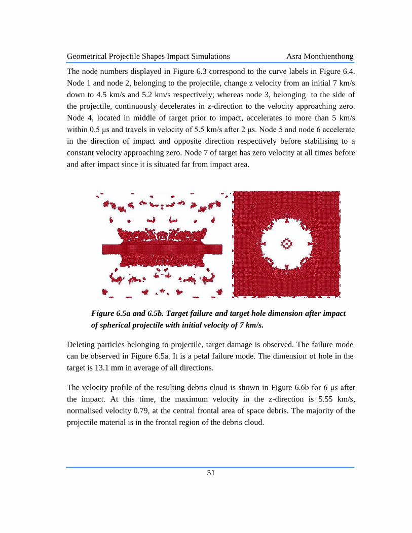
Figure 65a and 65b Target failure and target hole dimension after impact of spherical
projectile with initial velocity of 7 kms 51
Figure 66a and 66b debris cloud and its velocity profiles at 6 μs after impact of
spherical projectile with initial velocity of 7 kms 52
Figure 67a 67b and 67c Stress in z-direction at 01 μs 02 μs and 03 μs after impact
respectively of spherical projectile projectile with initial velocity of 7 kms
unit in 100 GPa 52
Figure 68a and 68b Full considered configuration and cross-section of cylindrical
projectile and thin plate target configuration respectively 53
Figure 69 Cross-section view of one quarter model of cylindrical projectile with
impact velocity of 7 kms at 05 μs 1μs and 2 μs after impact in left middle
and right respectively 54
Figure 610Cross-section of model illustrated the nodes and their numbers for
referencein plot Figure 611 55
Figure 611Nodal velocities in negative z direction of cylindrical projectile initial
velocity of 7 kms corresponded to nodes in Figure 610 55
Figure 612a and 612bTarget failure and target hole dimension after impact of
cylindrical projectile with initial velocity of 7 kms 56
Figure 613a and 613b Debris cloud and its velocity profiles at 6 μs after impact of
cylindrical projectile with initial velocity of 7 km 56
Figure 614Stress in z-direction at 01 μs 02 μs and 03 μs after impact of cylindrical
projectile with initial velocity of 7 kms unit in 100 GPa 57
Figure 615a and 615b Cubic projectile and thin plate target configuration and cross-
section of model with SPH particles respectively 58
Figure 616 Cross-section view of one quarter model of cubic projectile with impact
velocity of 7 kms at 05 μs 1μs and 2 μs after impact in left middle and
right respectively 58
Asra Monthienthong
vii
Figure 617 Cross-section of model illustrated the nodes and their numbers for reference
in plot Figure 618 59
Figure 618 Nodal velocities in negative z direction of cubic projectile initial velocity of
7 kms corresponded to nodes in Figure 617 59
Figure 619a and 619b Target failure and target hole dimension after impact of cubic
projectile with initial velocity of 7 kms 60
Figure 620a and 620b Debris cloud and its velocity profiles at 6 μs after impact of
cylindrical projectile with initial velocity of 7 kms 60
Figure 621 Stress in z-direction at 01 μs 02 μs and 03 μs after impact of cubic
projectile with initial velocity of 7 kms unit in 100 GPa 60
Figure 71 Comparison of debris cloud generated by spherical cubic and cylinder
projectiles (top middle and bottom) impact on thin plate at impact 3 μs and
6 μs after impact with impact velocity 7 kms 63
Figure 72 Comparison of velocity in impact direction of debris cloud generated by
spherical cubic and cylinder projectiles impact on thin plate at impact 6 μs
after impact with impact velocity 7 kms left middle and right respectively
64
Figure 73 Normalised maximum axial velocities at 6 μs after impact for each projectile
shape versus impact velocities 65
Figure 74a 74b and 74c Comparison of target of spherical cylindrical and cubic
projectiles in left middle and right respectively at 9 μs after impact with
impact velocity of 7 kms 66
Figure 75a 75b and 75c Stress in z-direction at 02 μs after impact of spherical
cylindrical and cubic projectile left middle and right respectively with
initial velocity of 7 kms 66
Asra Monthienthong
viii
List of Tables
Table 41 Material properties of Alminium 2024-T339
Table 42 Material properties of Alminium 2024-T340
Table 51 Spherical projectile impact on thin plate target configuration description for
validation 42
Table 52 Comparisons between experimental data and simulating data43
Table 71 Length and diameter of debris cloud at 6 μs after impact of initial velocity of
7 kms62
Table 72 Maximum axial velocities and normalised maximum axial velocities of 6 μs
after impact with impact velocity 7 kms64
Table 73 Majority of stress in z-direction at 02 μs and 03 μs after impact of spherical
cylindrical and cubic projectile left middle and right respectively with
initial velocity of 7 kms 67
Asra Monthienthong
ix
Nomenclature
A Area
E Internal energy
E0 Initial internal energy
T Temperature
Tlowast Homogenous temperature
V Volume
Vs Specific volume
U Shock velocity
up Particle velocity
v0 Initial velocity
c Wave velocity
ρ Material density
C0 Speed of sound in the material
W Kernel function
H Smoothing length
σ Stress
σlowast Ratio of pressure to effective stress
σy Yield stress
ε Strain
εlowast Non-dimensional strain rate
ε p Effective plastic strain
εf Strain at fracture
Asra Monthienthong
x
Abbreviations
SPH Smoothed Particle Hydrodynamics
MCM Meshless Continuum Mechanic
GEO Geostationary Earth Orbit
HEO Highly Elliptical Orbit
LEO Low Earth Orbit
NASA National Aeronautics and Space Administration
ESA European Space Agency
UN United Nations
Introduction Asra Monthienthong
1
1 Introduction
Geometrical shape projectile effects on hypervelocity impact are applicable to impact of
space debris to spacecraft The space debris threat is explained to aid in the
understanding of the confronting threat of spacecraft Spacecraft shielding systems and
the effect of space debris in general are described The objectives methodologies and
outline of the research are described in this chapter
11 Space Debris Threat
It has been more than 50 years since the beginning of space era starting at the first
Sputnik launch in 1957 Mankind continues launching and delivering spacecraft be it
rockets satellites shuttles or probes into the space Numerous parts of spacecraft are
abandoned in the space Their sizes may be as small as aluminium oxide particles from
solid rocket exhausts or fasteners to non-functioning satellite or launch vehicle upper
stages (Lacoste 2009) These objects that are abandoned near the Earth are still orbiting
around the Earth and become space debris All spacecraft will be confronted collision of
space debris and meteoroids during their function lifetime (Wertz et al 1999) The
collision may cause minor damage to major damage that can leads to the loss of mission
and spacecraft The level of damage depends on the size impact velocity impact angle
space debris density and so on The debris as small as 1 cm may cause serious damage
to spacecraft while particle sizes 01 cm may give rise to surface erosion in the long term
(Tribble 2003 and UN 1999)
12 Spacecraft Shielding System
Spacecraft shielding system is a passive mean to protect spacecraft against space debris
and meteoroids Shielding system is effective to protect spacecraft against objects
smaller than 1 cm in diameter (UN 1999) The simple and practical shielding system is
Whipple bumper shield that consists of a single thin plate called bumper placed at a
short distance ahead of a primary structure of the spacecraft pressure or rear wall (Chi
2008) The concept is to fragment andor vaporise the projectile through the impact with
the bumper typically metallic or composite thin plates Intensity of impulse is reduced
before the debris cloud of the projectile and bumper hits spacecraft structure and leads to
Introduction Asra Monthienthong
2
the loss of mission andor spacecraft The performance of shields is dependent on
distance between the bumper and the primary structure wall the material of the shield
the thickness of the shield and so on
Spacecraft shielding systems have been continuously developed varying both the
number of bumpers and the materials used The main concept is still to fragment andor
vaporise the projectile The resulting debris cloud expands and hits the next layer over a
larger area dispersing the energy of the projectile and the impulsive load (Campbell
1998) The characteristics of the debris cloud indicate the ability of the bumper of
fragmentation and vaporisation of the projectiles In designing spacecraft shielding
system it is crucial to comprehend debris cloud of the impact between of space debris
and the bumper
13 Effect of Space Debris Shapes
Spherical projectiles have been the conventional shape used in most of the experiments
and researches Morrison and Elfer (1988) have found cylinders with a length to
diameter ratio of 1 are much less penetrating than equivalent mass spheres at low impact
velocities of 3 kms but the ranking reversed at more than 6 kms (Elfer 1996) Elfer has
stated that this was because the cylinder shatters more easily than the sphere at 3 kms
At more than 6 kms in normal impacts the cylinder creates a debris cloud with a spike
of which the tip is the most lethal The tip appears to be a spall fragment from the
bumper normal to the flat of the cylinder that can penetrate the rear wall
Rolsten Hunt and Wellnitz (1964) found that significant differences in the impact pattern
of explosively-launched disc with different orientation in their studies of principles of
meteoroid protection Friend Murphy and Gough (1969) used polycarbonate cylindrical
and conical and cup-shaped projectile in their studies of debris cloud pressure
distribution on secondary surface Morrison (1972) proved that in particular cases a
cylindrical shape is more dangerous than spherical projectiles
Piekutowski (1987 1990) stated that the cylindrical projectiles are more efficient
penetrators of double-sheet structures than spherical projectiles of equivalent mass and
the incline cylindrical projectile causes more severe damage to the structure
Introduction Asra Monthienthong
3
Buyuk (2008) has studied ellipsoidal projectiles and compared the results of oblate and
prolate with sphere He concluded that it is not necessarily correct that the ideal
spherical projectiles are the most dangerous threat and also presented that the most
dangerous case of ellipsoidal projectiles orientation is not the case with the longest or
shortest side of the ellipsoidal projectiles parallel or perpendicular to the impact
direction
14 Research Objectives
Radar and ground-based studies of orbital space debris has discovered that orbital space
debris is not only composed of spheres Their sizes and shapes are varied (Williamsen
2008) Beside conventional studies in spherical projectiles studies are required for non-
spherical projectiles with different shapes in order to take them into account when
designing spacecraft shielding In this research the influence of projectiles with different
geometrical shapes is to be investigated Numerical simulations are applied due to their
advantages of inexpensiveness less man-power resource and time consuming in
comparison to actual experiments
The initial objective of this research is to investigate the effect projectile shape by
plotting ballistic limit curves for each projectile The first dual-wall structure was
constructed Its output file was 10 GB which was too large Plotting a ballistic limit
curve many simulations are required In order to observe characteristics of debris clouds
in different projectile shapes many curves are required
Study of debris cloud produced by projectile impact on the bumper can be used for
development of the method for approximating the pressure loading imposed on the rear
wall or spacecraft structure A spacecraft designer can estimate the response of a
structure by using the approximate pressure-loading history (Piekutowski 1990)
The main objective of this research is to investigate the influence of projectile shapes on
spacecraft shielding systems in the hypervelocity impact range The extended objectives
of this research are the following
- Simulate the impact of different shapes of projectiles on thin plate targets using
smoothed particle hydrodynamics methods
Introduction Asra Monthienthong
4
- Investigate the influence of different geometrical projectile shapes on debris
cloud characteristics and the fragmentation of projectiles with equivalent mass
impacting on thin plate target in hypervelocity impact
15 Research Methodologies
The methodologies of the research are
(i) Literature review for comprehension of the existing problems of space debris
and its threat its general background for defining scope objective
methodologies and further simulation set up for this research
(ii) Study the associated physical impact phenomena based on space debris impacts
on spacecraft shields or spacecraft
(iii) Study the methods used in the impact of projectiles in this range of velocity for
numerical simulation ie smoothed particle hydrodynamics methods
(iv) Set up a simulation based on available experimental data to validate numerical
simulation Validating numerical simulation by comparisons of characteristics
of debris cloud generated by numerical simulation and actual experiments
Accuracy of numerical simulation is calculated
(v) Simulate aluminium spherical cubic and cylindrical projectiles impacts on
single thin aluminium plates All projectiles are made of aluminium and have
equivalent mass Observe characteristics of debris cloud generated by each
geometrical projectile
(vi) Compare the characteristics of debris cloud generated by different projectile
shapes and finally conclude with suggested future work
Properties of debris cloud to be observed
- Debris cloud shape and size
- Debris cloud velocity profile and debris cloud velocities at particular points
- Target hole dimension and failure mode
- Impact induced stress
Introduction Asra Monthienthong
5
16 Research Outline
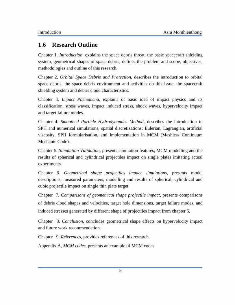
Chapter 1 Introduction explains the space debris threat the basic spacecraft shielding
system geometrical shapes of space debris defines the problem and scope objectives
methodologies and outline of this research
Chapter 2 Orbital Space Debris and Protection describes the introduction to orbital
space debris the space debris environment and activities on this issue the spacecraft
shielding system and debris cloud characteristics
Chapter 3 Impact Phenomena explains of basic idea of impact physics and its
classification stress waves impact induced stress shock waves hypervelocity impact
and target failure modes
Chapter 4 Smoothed Particle Hydrodynamics Method describes the introduction to
SPH and numerical simulations spatial discretizations Eulerian Lagrangian artificial
viscosity SPH formularisation and Implementation in MCM (Meshless Continuum
Mechanic Code)
Chapter 5 Simulation Validation presents simulation features MCM modelling and the
results of spherical and cylindrical projectiles impact on single plates imitating actual
experiments
Chapter 6 Geometrical shape projectiles impact simulations presents model
descriptions measured parameters modelling and results of spherical cylindrical and
cubic projectile impact on single thin plate target
Chapter 7 Comparisons of geometrical shape projectile impact presents comparisons
of debris cloud shapes and velocities target hole dimensions target failure modes and
induced stresses generated by different shape of projectiles impact from chapter 6
Chapter 8 Conclusion concludes geometrical shape effects on hypervelocity impact
and future work recommendation
Chapter 9 References provides references of this research
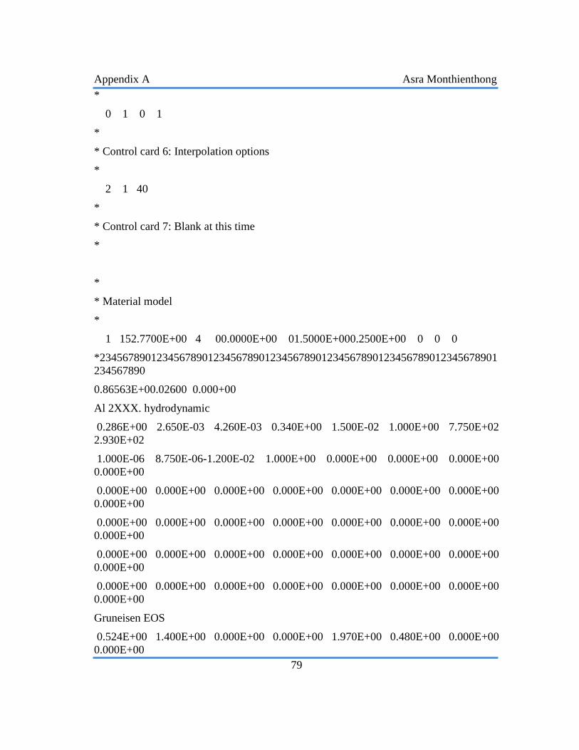
Appendix A MCM codes presents an example of MCM codes
Space Debris and Protection Asra Monthienthong
6
2 Orbital Space Debris and Protection
In this chapter space debris and protection against it are explained The studies in space
debris are divided into three main topics which are measurements modelling amp risk
assessment and mitigation The characteristic length of space debris is explained The
spacecraft shielding system is introduced and its development is explained The ballistic
limit curve is described
21 Introduction to Orbital Space Debris
Orbital space debris also called space debris space junk or space waste is the man-
made objects which is no longer used (UN 1999) generally refer to it as the results of
space missions no longer serving any functions anymore This has drawn attention to
many authorities and organisations around the world that are aware of the growth of
space debris and its threat to spacecraft Space debris is orbiting around the Earth with
very high velocity
Figure 21 Trackable objects in orbit around the Earth (ESA 2008)1
In Figure 21 the illustration of the trackable objects in orbit around the Earth by
European Space Agency is shown Space debris population is densest in Low-Earth
Orbit (LEO) and Geostationary Orbit (GEO) which are the orbits that are used for Earth
observation and communication The growth of space debris population in LEO is
Space Debris and Protection Asra Monthienthong
7
approximately 5 percent per year With the effort of all nations and many organisations
in the last few decades it is expected that the growth of the space debris population will
decrease and the amount space debris will be mitigated This mitigating effort can be
achieved by de-orbiting to the atmospheric drag placing spacecraft in disposal or
graveyard orbits and so on (NASA 2005)
Figure 22 Spatial density of space debris by altitude according to
ESA MASTER-2001(Wiki Michael Oswald 2004)2
The elaboration of space debris density is graphed in Figure 22 The impact velocities
of space debris are dependent on the orbiting altitude (Committee on Space Shuttle
MeteoroidsDebris Risk Management 1997) Space debris in LEO is travelling with
higher velocity than debris in GEO Thus the impact velocity of space debris in LEO
approximately betwen10-15 kms is higher than that in GEO which is approximately 05
kms To visualise this velocity range one can compare with objects on Earth such as
bullet The rifle bullet velocity is between 10 and 15 kms (Pereyra M 1999)
Therefore impact velocity in LEO is roughly 10 times higher that riffle bullets velocity
According to NASA (2009) 1-centimeter of aluminium travelling at this range of
velocity may cause damage as harmful as 400-lb safe travelling at 60 mph Figure 23
shows the growth of space debris population in the last four decades
Space Debris and Protection Asra Monthienthong
8
Figure 23 Growth of space debris population model (ESA 2008)3
22 Study in Space Debris
Space debris has been studied in three main aspects according to United Nation
conference in New York USA 1999 The space debris problem has been investigated
and divided in three main categories (UN 1999) which are space debris measurement
space debris modelling amp risk analysis and space debris mitigation
221 Space Debris Measurement
Space debris is tracked and monitored Tracking can be performed using either ground-
based systems or space-based systems Generally ground-based systems are capable to
track space debris of size 10 cm or larger and space-based systems are able to track
space debris of size 1 cm or larger (Tribble 2003)
Ground-based measurement systems have two main categories of measurement which
are radar measurement and optical measurement The radar measurement can be
performed in all weather and in both day and night time but it is limited to small objects
in long range (UN 1999) whereas optical measurement needs to be performed while the
space debris is sunlit and the background sky is dark Therefore the observation in LEO
can be performed in limited periods of the day while in HEO (High-Earth orbit) it can be
performed at all times of the day According to ESA 2009 (Lacoste 2009) radar
measurements are suitable for the LEO regime below 2000 km Optical measurements
are suitable for GEO and HEO observations
Space Debris and Protection Asra Monthienthong
9
Space-based measurement systems have two categories The first is retrieved surfaces
and impact detectors approached by analysing the exposed spacecraft surface to the
space environment after its return to Earth Examples of well-known projects of this type
of measurement are Long-Duration Exposure Facility (LDEF) European Retrievable
Carrier (EURECA) etc The second category uses sensors to measure impact fluxes and
the meteoroid and space debris population Space-base measurement has higher
resolution and performance than ground-based systems with the trade-off of higher cost
Examples of this space-based measurement are DEBIE (Debris In-Orbit Evaluator)
launched in 2001 and DEBIE II launched in 2008 Infra-red Astronomical Satellite
(IRAS) in 1983 MSX spacecraft in 1996 and Geostationary Orbit Impact Detector
(GORID) in 1996
Cataloguing is where a record is taken of orbital space debris population characteristics
that have been derived from measurement or record The United States Space Command
catalogue and the space object catalogue of Russian Federation are space debris
catalogues that are frequently updated ESA has the Database Information System
Characterising Objects in Space (DISCOS) which is base on those two catalogues
belonging to the United States and the Russian Federation
222 Space Debris Modelling and Risk Assessment
Models of space debris environment rely upon historical data and are limited by the
sparse amount of data available to validate the derived characteristics Space debris
models have been continuously developed by various organisations such as EVOLVE
by the NASA Johnson Space Center and MASTER by ESA
Space debris risk assessment is divided into collision risk assessment and re-entry risk
assessment Collision risk assessment is utilised to enhance safety of space operation
designing spacecraft with pre-flight risk assessment within acceptable levels It is also
used to design the type and location of space debris shielding to protect the crew and
critical subsystems and components Re-entry risk assessment is the assessment of the
chance of uncontrolled re-entry from the Earth orbit
Space Debris and Protection Asra Monthienthong
10
223 Space Debris Mitigation
Mitigation consists of two main concepts which are not to make the existing problem
worse and for a reduction of the rate of increase of space debris over time to strive to
protect the commercially valuable low Earth and geostationary orbits through protection
strategies (ESA 2009)
Reduction in the rate of increase of space debris has three approaches First avoidance
of debris generated under normal operation resulting making the existing problem
worse Second prevention of on-orbit break-ups is by preventing on-orbit explosion and
collision Third de-orbiting and re-orbiting of space objects
Figure 24 Space debris sizes and protection methods 4
Protection of spacecraft can be achieved by both shielding and collision avoidance
Space debris shielding is quite effective against small particles Particles smaller than
01 cm can cause erosion in the long term but no serious immediate damage (Tribble
2003 amp Vedder 1976) Figure 24 shows protection of spacecraft against space debris
with respect to space debris size Typical space debris shields can protect spacecraft
structures against particles 01 to 1 cm in size All objects 1 to 10 cm in size cannot
currently be blocked by shielding technology nor be tracked for collision avoidance by
operational means Nonetheless risk analysis has very much concern in the range of
space debris size that spacecraft shielding cannot protect against The risk of being
impacted by space debris size 5 mm is 0005 time per ten-day mission (Committee on
Space Shuttle MeteoroidsDebris Risk Management 1997) Therefore risk analysis is
the only available solution for space debris of sizes between 1 to 10 cm Space debris
sizes larger than 10 cm are trackable by ground-based systems In addition protection
Space Debris and Protection Asra Monthienthong
11
against objects 1 to 10 cm in size can be achieved through special features in designing
of spacecraft systems such as redundant systems frangible structures pressure vessel
isolation capabilities etc
23 Characteristic Length of Space Debris
To define different shapes of space debris for radar detection characteristic length is a
parameter characterized size of space debris developed by NASA (Hill et al 2008))
Characteristic length is defined as
119871 =119883 + 119884 + 119885
3
Where X Y and Z are the maximum orthogonal projections of object
It has been used for the detectable radar cross-section The characteristic length of
sphere is its diameter For a cube the characteristic length is its dimensions in length
width and thickness If spherical and cubic space debris are made of identical material
then they possess equivalent mass and volume The cubic space debris has a smaller
characteristic length and less detectable than spherical space debris
24 Spacecraft Shielding System
Beside man-made space debris meteoroids which are natural objects in the solar system
(Wiki 2009) may collide with the spacecraft and consequently cause damage to the
spacecraft The meteoroid threat has been a concern since the beginning of human
spaceflight when the space debris has not yet accumulated and become an important
issue of space hazards Nevertheless collision of meteoroids is less harmful to the
spacecraft in comparison with the collision of space debris due to the fact that the
density of the meteoroids is much less than space debris even though impact velocity of
meteoroids may be higher (Jolly 1997) Hence the key to design spacecraft in order to
withstand both space debris and meteoroids is to consider the impact of space debris to
spacecraft or its shielding system
241 Shielding System Development
The first spacecraft shielding against meteoroids and space debris was introduced by
Fred Whipple in 1947 which is still being used until present day (Jolly 1997) The
Whipple bumper shield has one outer bumper placed at the short distance ahead of a
Space Debris and Protection Asra Monthienthong
12
primary structural system The concept is to fragment andor vaporise the projectile
through the impact with the bumper typically metallic or composite thin plates The
main concept is to fragment or vaporise the projectile The resulting the debris cloud
expands and hits the next layer over a larger area dispersing the energy of the projectile
and the impulsive load The Whipple bumper shocks the projectile and creates a debris
cloud containing smaller less lethal bumper and projectile fragments The full force of
debris cloud is diluted over a larger area on the spacecraft rear wall
Figure 25 Whipple bumper shield after impact of projectile (left) and rear wall of
a Whipple shield impacted fragmentation of projectile and bumper (right)(Hyde
HITF2009) 5
Spacecraft shielding has been continuously developed Various materials are adopted to
apply in spacecraft shielding system for examples aluminium Nexteltrade Kevlarreg
aluminium mesh aluminium honeycomb sandwiches etc The basic idea of
fragmenting and vaporising a projectile is also applied to other shielding systems that
have been developed after Whipple bumper shield such as stuffed Whipple shield mesh
double bumper shield and multi-shock shield (Schonberg 1999)
Figure 26 Stuffed Whipple shield after impact of a projectile (left) and mesh
double bumper shield after impact of a projectile (right) (Hyde HITF2009)6
Space Debris and Protection Asra Monthienthong
13
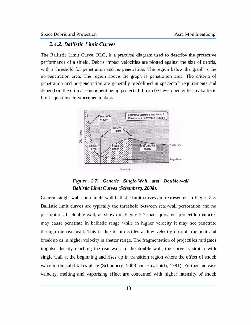
242 Ballistic Limit Curves
The Ballistic Limit Curve BLC is a practical diagram used to describe the protective
performance of a shield Debris impact velocities are plotted against the size of debris
with a threshold for penetration and no penetration The region below the graph is the
no-penetration area The region above the graph is penetration area The criteria of
penetration and no-penetration are generally predefined in spacecraft requirements and
depend on the critical component being protected It can be developed either by ballistic
limit equations or experimental data
Figure 27 Generic Single-Wall and Double-wall
Ballistic Limit Curves (Schonberg 2008) 7
Generic single-wall and double-wall ballistic limit curves are represented in Figure 27
Ballistic limit curves are typically the threshold between rear-wall perforation and no
perforation In double-wall as shown in Figure 27 that equivalent projectile diameter
may cause penetrate in ballistic range while in higher velocity it may not penetrate
through the rear-wall This is due to projectiles at low velocity do not fragment and
break up as in higher velocity in shatter range The fragmentation of projectiles mitigates
impulse density reaching the rear-wall In the double wall the curve is similar with
single wall at the beginning and rises up in transition region where the effect of shock
wave in the solid takes place (Schonberg 2008 and Hayashida 1991) Further increase
velocity melting and vaporising effect are concerned with higher intensity of shock
Space Debris and Protection Asra Monthienthong
14
propagate into the projectile and target consequently some energy is left causing change
of state (Piekutowski 1990)
25 Debris Cloud Characteristics
Piekutowski (1996) has described the debris cloud produced by spherical projectiles as
composing of three major features which are ejecta external bubble of debris and
internal structure An ejecta veil is ejected from the impact side of bumper and almost
entirely composes of bumper An expanding bubble of bumper debris forms at the rear
side of the bumper The internal feature consists of projectile debris located inside and at
the front of the external bubble of bumper debris
Figure 28 Debris cloud structure produced by spherical projectile
(Piekutowski 1996) 8
The velocities of debris cloud after impact is widely represented in terms of normalised
velocities which are the ratio of local velocities of debris cloud to impact velocity of
projectile
Space Debris and Protection Asra Monthienthong
15
Figure 29 Debris cloud structure produced by
cylindrical projectile (Piekutoski 1987) 9
Debris produced by cylindrical projectiles has structures as shown in Figure 29 It
consists of the main debris cloud inner cone and front cone Piekutowski 1987
performed experiments using copper as a bumper material and an aluminium cylindrical
projectile He found that the front cone of debris cloud consists of bumper material
The population of space debris has continuously grown Spacecraft are threatened by
collision of space debris The spacecraft shielding system has been developed due to the
fact that all spacecraft confronts collisions of space debris and micrometeoroids Studies
on space debris have been performed in three main categories which are space debris
measurement modelling amp risk analysis and mitigation Characteristics of debris clouds
are different for different projectile shapes
The following steps after understanding the problems and the main features concerned
with the topic is to study the associated physical impact phenomena that will be
presented in the next chapter
Impact Phenomena Asra Monthienthong
16
3 Impact Phenomena
The brief explanations of impact phenomena impact physics hypervelocity impact and
failure modes are presented Comprehension of impact phenomena is crucial for
understanding and performing simulation of hypervelocity impact This chapter starts
with classification of impact phenomena The impact physics section explains the
mechanism properties and characteristics of impact Hypervelocity impacts which are
in the interest of this research are described Finally target failure modes are explained
31 Classification of Impact Phenomena
Impact Phenomena can be classified as elastic and inelastic impacts Elastic impact is
where there is no loss of translational kinetic energy ie no translational kinetic energy
is dissipated into heat nor converted to neither rotation kinetic vibration nor material
deformation energy (Vignjevic 2008) The inelastic impact is on the other hand where
translational kinetic energy exists In this research it is focused on inelastic impact The
impact of deformable bodies influenced by stress wave propagation and inertia effects is
called impact dynamics
Impact dynamics has two main features that are different from the classical mechanics of
deformable bodies which are the influence of stress wave propagation in the material
and the importance of inertia effects that have to be taken into account in all of the
governing equations based on the fundamental laws of mechanics and physics
Generally impacts are transient phenomena where steady states conditions never take
place
32 Impact Physics
Impact physics of hypervelocity projectiles impacting on a thin plate is the interest of
this research The concerned mechanism and phenomena of such impact are discussed in
this section The basic stress wave and its propagation mechanism are described Stress
induced by impact is explained
Impact Phenomena Asra Monthienthong
17
321 Stress Wave
Stress waves are stresses that transfer within the material bodies from impacting surfaces
inward to material bodies The collision generates stresses in the material of the bodies
that must deform in order to bear these stresses The stresses and deformations do not
immediately spread through all of material bodies Compression forces particles closer
together which takes time and requires relative motion Stresses and deformations are
transmitted from the impacting surface to all parts of the bodies in the form of waves
Stress wave mechanism is illustrated in Figure 31 one-dimensional compressive stress
wave propagation Assume that an unstressed bar is exposed suddenly to a pressure that
remains constant thereafter The bar is assumed to be composed of a large number of
very thin layers of particles parallel to the impact plane Considering one-dimension
wave propagation numbers within the particles represent layer numbers of particles
Immediately after impact the pressure is supported entirely by inertia of the first particle
which is particle at the surface The first particle is accelerated The spring between first
and second particle is compressed as the first particle moves toward second particle
Compressive stress from the spring accelerates second particle The second particle
moves and the spring between second and third particle is compressed Compressive
stresses build and accelerate consecutive particles forming a stress wave
Figure 31 One-dimensional compressive stress wave propagation (Lepage 2003) 10
Stress waves reflect when they encounter boundaries Similar to general waves stress
waves reflect in opposite phase when encountering free boundary The phase of
reflecting waves remain unchanged when encountering fixed boundary In compressive
stress waves encountering a free boundary the reflecting waves are tensional stress
Impact Phenomena Asra Monthienthong
18
waves On the other hand compressive stress waves reflected as compressive stress
waves when encountering a fixed boundary (Zukas 1982)
Considering the propagation of a uni-axial stress wave in a bar for small strains and
displacements from non-deformed shape free body diagram is shown in Figure 32
Figure 32 Free-body diagram of an element dx
in a bar subject to a stress wave in x-direction 11
Applying Newtonrsquos second law to the element dx
120589 +120597120589
120597119909119889119909 minus 120589 119860 = 120588119889119909119860
120597119907
120597119905 (31)
Equation (31) is simplified and can be written
120597120589
120597119909 = 120588
120597119907
120597119905 (32)
The continuity condition derives from the definitions of strain and velocity
휀 =120597119906
120597119909 and 119907 =
120597119906
120597119905 (33a) and (33b)
The Equation (33a) and (33b) can be written
120597휀
120597119909=
1205972119906
1205971199092 and 120597119907
120597119905=
1205972119906
120597119905 2 (34a) and (34b)
Impact Phenomena Asra Monthienthong
19
Left-hand side of Equation (32) can be written
120597120589
120597119909 =
120597120589
120597휀∙120597휀
120597119909=
120597120589
120597휀 ∙
1205972119906
1205971199092 (35)
Substituting Equation (34) and (35) stress wave equation is obtained
part2u
partt2=c2 part
2u
partx2 (36)
Where 119888 = 119878
120588 is the wave velocity and S is slope of stress-strain curve
If stress applied to material is lower than yield strength stress waves generated are in
elastic region called elastic stress wave In the elastic region S is the Youngrsquos modulus
of material In the plastic region where applied stress is more than yield strength of
material plastic stress waves are generated Usually the slope of stress-strain curve in
plastic region is lower than in elastic region Therefore the stress wave velocity in
plastic region is lower than one in elastic region Nevertheless some cases exist where
the stress-strain curve in plastic region concaves up The plastic stress wave velocity is
higher than one of elastic stress wave and consequently there is a single plastic shock
wave in the material (Vignjevic 2008)
322 Impact Induced Stress
Once impact occurs stress and strain are induced in material starting from the impact
surface and transmit inward material bodies Stress and strain are induced through the
material bodies Induced stress and strain in material by impact can be estimated by
applying fundamental conservation laws and wave propagation concepts
To analyse impact induced stress and strain the event of a moving rigid wall impacting
a stationary bar are considered This analysis is the same as a moving bar impacting a
stationary wall First considering the rigid wall travels at initial velocity v0 and bar is at
rest At the time dt after impact the rod will be deformed with distance v0 dt The
original surface is deformed to plane A The impact induced strain up to plane A at time
dt Disturbance in the bar at time dt reaches plane B the material of the bar behind plane
B is undisturbed and has no velocity and no stress induced The distance from original
surface of the bar to plane B is c dt where c is the wave velocity The impact induced
stress up to plane B at time dt
Impact Phenomena Asra Monthienthong
20
Figure 33 Illustration of stress-strain induced by impact between rigid wall and bar 12
Illustration of impact between rigid wall and bar is shown in Figure 33 Applying law of
conservation of momentum to analyse impact between rigid wall and bar impulse
transmitted to the rod is σ A dt where A is cross section of the bar The change of
momentum is the product of mass and velocity of all particles under disturbance
between original surface of the bar to plane B which is ρ A cdt vo The force impulse is
equal to change of momentum
120589 119860 119889119905 = 120588 119860 119888119889119905 1199070 (37)
Equation (37) can be simplified to obtain impact-induced stress
120589 = 1205881198881199070 (38)
This impact-induced stress in Equation (38) is derived for the case that the rod is
initially at rest and unstressed The impact of a moving projectile on stationary target is
the interest of this research The projectile and target are made of the identical material
and therefore have the identical properties ie identical material density and stress wave
velocity If the velocities in the material are measured with respect to the impact
interface the interface can be considered as a rigid surface to projectile and target At
the interface stress magnitude in the projectile is equivalent to one in the target
1205891 = 1205892119905 (39)
Impact Phenomena Asra Monthienthong
21
Where subscripts 1 and 2 refer to of projectile and target respectively
Equation (39) can be written
120588111988811199071 = 120588211988821199072 (310)
The particle velocity in the projectile v1 and particle velocity in the target v2 are relative
to the interface Therefore the sum of particle velocities after impact is equal to initial
velocity of projectile before impact and it can be written as
1199070 minus 1199071 = 1199072 (311)
Substitute Equation (311) to Equation (310) Material density and wave velocity in
material are the same since both the projectile and the target are made of the same
material Hence the impact is symmetrical and magnitudes of particle velocity in
projectile and in target are equal The relationship between magnitudes of velocities can
be written as
1199071 = 1199072 =1199070
2 (312)
The impact-induced stress can be expressed as a function of the material properties and
impact velocity
120589 = 1205881198881199070
2 (313)
Equation (313) is used to predict the impact-induced stress
323 Shock wave
Shock wave is a type of propagating disturbance carrying energy through the medium It
is crucial to comprehend the basic idea of the shock wave It leads to shock in solids
which is an important feature to study in hypervelocity impact Shock waves are an
integral part of dynamic behaviour of materials under high pressure Shock waves form
discontinuity in the medium between in front of and behind the shock wave as shown in
Figure 34 (Campbell 1994)
Impact Phenomena Asra Monthienthong
22
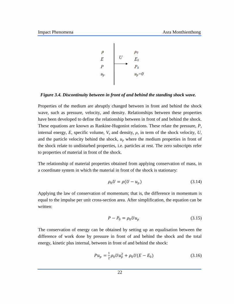
Figure 34 Discontinuity between in front of and behind the standing shock wave13
Properties of the medium are abruptly changed between in front and behind the shock
wave such as pressure velocity and density Relationships between these properties
have been developed to define the relationship between in front of and behind the shock
These equations are known as Rankine-Hugoniot relations These relate the pressure P
internal energy E specific volume Vs and density ρ in term of the shock velocity U
and the particle velocity behind the shock up where the medium properties in front of
the shock relate to undisturbed properties ie particles at rest The zero subscripts refer
to properties of material in front of the shock
The relationship of material properties obtained from applying conservation of mass in
a coordinate system in which the material in front of the shock is stationary
1205880119880 = 120588(119880 minus 119906119901) (314)
Applying the law of conservation of momentum that is the difference in momentum is
equal to the impulse per unit cross-section area After simplification the equation can be
written
119875 minus 1198750 = 1205880119880119906119901 (315)
The conservation of energy can be obtained by setting up an equalisation between the
difference of work done by pressure in front of and behind the shock and the total
energy kinetic plus internal between in front of and behind the shock
119875119906119901 =1
21205880119880119906119901
2 + 1205880119880(119864 minus 1198640) (316)
Impact Phenomena Asra Monthienthong
23
Substitute up and ρ0U from laws of conservation of mass and momentum Equation in
(314) and (315) and replace 1ρ by V then simplifying The Hugonoit energy equation
is obtained
119864 minus 1198640 =1
2 119875 + 1198750 1198810 minus 119881 (317)
These equations involve five variables ie ρ σ E u and U Hence there are two
independent variables The Hugoniot curve is a material property that is the locus of
attainable shock states and is equivalent to a stress-strain curve if uni-axial stress is used
as the fourth equation Therefore knowledge of one of any variables with application of
these four equations is sufficient to determine other variables
The simplest form of Hugoniot curve is a diagram where shock velocity is a function of
particle velocity This can be obtained from the impact of two identical flat plates The
particle velocity behind the shock is half the impact velocity The relationship between
shock velocity and particle velocity has been found to be linear in many materials
119880 = 1198620 + 1198781119906119901 (318)
Where S1 is experimentally determined material constant and C0 is the speed of sound in
the unstressed material
Figure 35 Example of Hugoniot Curve representing material behaviour under a
uniaxial strain state (Campbell 1994) 14
Shock waves will be not be generated if the impulsive load is not large enough An
elastic or elastic-plastic wave will be generated and propagate through the material
Impact Phenomena Asra Monthienthong
24
Figure 35 shows an example of Hugoniot curve At low pressure the curve is linear and
the wave travels through the material as an elastic wave The point where the linear
relationship of Hugoniot curve ends is the Hugoniot Yield Stress or Hugoniot Elastic
Limit
33 Hypervelocity Impact
Hypervelocity impact is significant for studying space debris impacting on spacecraft
and its further application to spacecraft protection design Spacecraft encounter space
debris and micrometeoroids most of them travelling in the hypervelocity region
Hypervelocity impact usually occurs in the region where impact velocity is higher than
speed of sound in the collision materials (Zukas 1982) It refers to velocities so high that
the strength of materials upon impact is very small compared to inertial stresses For
aluminium hypervelocity impact is of order of 5 kms and higher
Hypervelocity impact creates a crater which results from a solid target melting and
vaporising Targets and projectiles behave like fluid and crater parameters depend more
on projectile and target densities and impact energy Hence the principal of fluid
mechanics may be used at least for starting of hypervelocity impact analysis
Hypervelocity impact can be classified into 3 categories based on target thickness which
are semi-infinite target intermediate thickness target and thin target
An impact into semi-finite target is one that has no stress wave reflection effect on the
pulverisation of the projectile and target from the rear side of the target Shock waves
are generated after the projectile impacts on the target where peak stresses are largely
higher than material strength Projectile impact causes a crater in the target The crater
shape depends on the shape of projectile and materials present The chucky projectile
such as sphere or cube will create a hemispherical crater The longer projectile will
create a deeper crater
An impact into intermediate thickness target concerns the effect of stress wave reflection
on the pulverisation of the projectile and target from the rear side of the target When
primary compressive stress shock waves detach from the expanding crater surface and
reach rear side of the wall which is a free surface the waves reflect as tensional stress
waves back The tensional stress waves are generated to satisfy the condition of stress at
Impact Phenomena Asra Monthienthong
25
any free surface remains zero at all time They travel backward into the target in the
opposite direction of compressive stress waves The instantaneous pressure at any point
in the target is the algebraic sum of forward running compressive stress wave and
rearward running tensile stress wave When the pressure at any point exceeds ultimate
dynamic tensile-yield strength the target at that point will fracture The spallation or
spall of rear surface of the target is formed with depth approximately one third of target
thickness The crater growth begins at the front surface of the target and continues until
approximately two thirds of the target thickness where its floor meets the uppermost
spall plane resulting in target perforation This situation is known as lsquoballistic limit
conditionsrsquo
Figure 36 Wave propagation and perforation mechanism in
intermediate thickness target (Zukas 1982) 15
An impact into thin targets has similar results to impacts into intermediate thickness
targets There is an effect of stress wave reflection on the pulverisation The energetic
projectile penetrates through the thin target plate with only small fraction of projectile
kinetic energy to form perforation in the target The shock waves propagate forward into
the target and backward into the projectile until they confront the free surface of the
target or projectile The shock wave in the target generally reflects as a tensile stress
wave back into target when encountering a free surface of the rear surface of the target
Meanwhile a primary shock wave in the projectile may encounter a side and rear
surface of projectile and reflects as tensile stress wave back into the projectile
Thin plates are used as bumpers to protect spacecraft from space debris Fragmentation
melting and vaporisation of the projectile and target reduce the intensity of impulse of
impact before impacting to spacecraft This concept is applied to spacecraft shielding
system
Figure 37 depicts the mechanism of projectile impact into a dual-wall structure
Projectile fragmentation melting and vaporisation of the projectile and the bumper
Impact Phenomena Asra Monthienthong
26
reduce the intensity of impulse of projectile impact before striking to spacecraft
Vaporised cloud and particles of bumper and projectile disperse over a large area of the
rear wall or spacecraft wall depending on standoff distance etc Individual craters in the
rear wall may be generated Spalling or spallation may occur as the rear wall can be
considered as an intermediate thickness target or thin target The criteria of failure of
rear wall are different depending on each predefine failure of the mission
Figure 37 Normal Impact of a Dual-Wall Structure (Schonberg 1991) 16
34 Target Failure Mode
Failure can occur in various modes It depends on each mission and component critical
criterion whether a target is identified as failure Failure occurs in different modes
depending on several characteristics of both the projectile and target such as impact
velocity and obliquity geometry of projectile and target and material properties A target
may fail in one failure mode or in combination of many failure modes Figure 38
depicts target failure modes that mostly occur in projectile impact on the thin to
intermediate thickness target
Fracture occurs due to the initial compression stress wave in a material with low density
Radial fracture behind initial wave in a brittle target of its strength is lower in tension
Impact Phenomena Asra Monthienthong
27
than in compression Spall failure occurs due to the reflection of initial compression
wave as tension causing a tensile material failure Plugging is formed due to the
formation of shear bands Frontal and rearwards petaling is the result of bending
moment as the target is pushed Fragmentation generally occurs in case of brittle
targets Hole in ductile material is enlarged (Corbett 1996 and Lepage 2003)
Figure 38 Failure modes of various perforation
mechanisms (Backman 1978) 17
Impact phenomena in hypervelocity impacts are concerned with stress wave propagation
and shock waves in solids Target failure modes are different for each material of
impact geometry of problem impact velocities and obliquity The next step is to apply
physical phenomena into simulation The development of the method used for
simulation is explained in the following chapter
Smoothed Particle Hydrodynamics Method Asra Monthienthong
28
4 Smoothed Particle Hydrodynamics Method
To perform a simulation properly comprehension of the numerical simulation technique
is required Smoothed Particle Hydrodynamics (SPH) method is implemented to the
simulations in this research This chapter presents the basic description of SPH and a
short history concerned with its application in hypervelocity impact simulation The
procedures of numerical simulation are provided Important features of the method are
explained ie spatial description time integration artificial viscosity and
formularisation Finally the implementation in MCM is explained
41 Introduction to SPH and Numerical Simulation
Smoothed Particle Hydrodynamics (SPH) is a gridless Lagrangian method The mesh-
free property is the main difference between SPH and classical finite element method It
was developed for simulations of extreme deformation and high pressure in which
classical finite element the mesh tangling exists It uses hydrodynamics computer codes
or hydrocodes which are used to simulate dynamic response of material and structure to
impulse and impact with large deformation (Hallquist 2006 and Hyde 2008) The
solution is obtained by applying physical continuum equations Computational grids are
generated in both space and time SPH divides the fluid into a set of discrete elements
The discrete elements are referred as particles These particles have a spatial distance
so-called smoothing length Properties of particles are smoothed by kernel function
Physical quantity of any particle can be obtained by summing the relevant properties of
all particles that are located within smoothing length
Smoothed Particle Hydrodynamics was first introduced by Lucy Gingold and
Monaghan in 1977 originally to simulate problems in astrophysical phenomena Later
it has been widely applied in continuum solid and fluid mechanics such as fluid
dynamics to simulate ocean waves aerodynamics and gas dynamics Libersky and
Petschek (1990) applied SPH to elastic-plastic solid by adding of strength effects to
simulate hypervelocity impact An axisymmetric model of SPH was introduced in 1993
(Petschek and Libersky 1993 Joshson 1993) by ignoring the hoop stresses at axes and
representing a smoothed torus of material about the axes of symmetry The three-
Smoothed Particle Hydrodynamics Method Asra Monthienthong
29
dimensional algorithm and SPH node linkage with standard finite element grids are
developed by Johnson (1993)
The procedure of conducting a numerical simulation is described in the diagram in
Figure 41 It begins with observation of physical phenomena followed by establishing a
mathematical model with some simplifications and necessary assumptions The
mathematical model can be expressed in ordinary differential equations (ODE) or partial
differential equations (PDE) as governing equations The boundary condition (BC) and
initial condition are required to specify properly in space andor time Geometries of
problems are divided into discrete components in order to numerically solve the
problems The technique of discretization is different for each method Coding and
implementation of numerical simulation for each problem are applied The accuracy of
numerical simulation is dependent on mesh cell size initial and boundary condition and
others applied earlier (Liu et al 2003)
Figure 41 Procedure of conducting numerical simulation (GR Liu amp MB Liu 2003)18
42 Spatial Discretization
Geometries or materials in finite element techniques are divided into small
interconnected sub-regions or elements in order to determine the solution with
differential equations The spatial discretization or mesh of space is basically divided
into two categories which are Eulerian method and Lagrangian method
Smoothed Particle Hydrodynamics Method Asra Monthienthong
30
421 Eulerian Method
In an Eulerian mesh the mesh or grid is fixed and coincident with spatial points as
material flows through it as shown in Figure 42a All the mesh nodes and cell
boundaries remain fixed in the mesh at all time Mass momentum and energy flow
through the cell boundaries The new properties of each cell are calculated from the
quantities of flow into and out of the cell Only current properties are available The time
history of particular particles cannot be tracked Eulerian mesh has to be applied in all
working space even there is no material in such cell This requires more CPU time than
Lagrangian mesh
422 Langrangian Method
In Lagrangian mesh the mesh or grid is coincident with a material particular point The
mesh or grid moves along with material at all time as shown in Figure 42b The element
deforms with the material Therefore each particular point of material can be tracked
The calculation in Lagrangian mesh can be performed faster due to the fact that
calculation is performed only where material exists
Figure 42a and 42b 2-D Eulerian mesh and Lagrangian mesh left
and right respectively (Zukas 1990) 19
Smoothed Particle Hydrodynamics Method Asra Monthienthong
31
It is suitable for problems with high distortion However the distortion of the mesh and
mesh tangling may occur in extremely high deformation Elements which experience
high distortion may cause instabilities and abnormal simulation termination
423 Alternative Method
To avoid the disadvantages of Eulerian and Lagrangian method there have been
researches to develop a method which would combine the advantages of both Arbitrary
Lagrangian Eulerian method is a method which its nodes can be programmed to move
arbitrarily Therefore the advantages of both Eulerian and Lagrangian can be exploited
Usually the nodes on the boundaries are moved to remain on the boundaries while the
interior nodes are moved to minimise mesh distortion The element erosion method
which deletes the heavily distorted elements from the material has been added to
conventional Lagrangian method The SPH method adds the meshless property to
conventional Lagrangian method as described earlier
43 Artificial Viscosity
Numerical simulations in hypervelocity impact are always concerned with shock waves
Discontinuity between regions in front of and behind the shock is a problem causing
unstable oscillations of flow parameters behind the shock This problem is solved by
adding the artificial viscosity to in term q to pressure to mitigate the discontinuities in
the regions between in front of and behind the shock This artificial viscous term q
damps out the oscillation behind the shock (Hiermaier 1997)
The viscous term q is usually expressed in term of quadratic function which is 휀119896119896 the
trace of the strain tensor (Hallquist 1998)
119902 = 120588119897 1198620119897휀1198961198962 minus 1198621119888휀 119896119896 for 휀 119896119896 lt 0 (41)
119902 = 0 for 휀 119896119896 ge 0 (42)
Where C0 and C1 are the quadratic and linear viscosity coefficients which has
default value of 15 and 006 respectively
c is the local speed of sound l is the characteristic length
Smoothed Particle Hydrodynamics Method Asra Monthienthong
32
44 SPH Formularisation
Properties of materials in the Smoothed Particle Hydrodynamics method are smoothed
by the interpolation formula and kernel function instead of obtain by divided grids The
function f(x) at the position x is an integration of function f of neighbouring positions xrsquo
times an interpolating kernel function 119882(119909 minus 119909prime 119893)
119891 119909 = 119891 119909prime 119882 119909 minus 119909prime 119893 119889119909prime (43)
Where h is a smoothing length
119891 119909 is a kernel approximation of function 119891 119909
The brackets referred to kernel approximation
The consistency of the kernel function is necessary Therefore the kernel function is
required to have a compact support which is zero everywhere but in the finite domain
within the range of smoothing length 2h as in Equation (44) The smoothing length and
set of particles within it are depicted in Figure 43 The kernel function is required to be
normalised as in Equation (45)
119882 119909 minus 119909prime 119893 = 0 for 119909 minus 119909prime ge 2119893 (44)
119882 119909 minus 119909prime 119889119909prime = 1 (45)
Figure 43 Smoothed particle lengths and set of particle within (Colebourn 2000)
20
Smoothed Particle Hydrodynamics Method Asra Monthienthong
33
Consistency requirements were formulated by Lucy (1977) to ensure the kernel function
is a Dirac function if h is zero or approaching to zero and the kernel function 119891 119909 is
equal to f(x) if smoothing length is zero
lim119893rarr0 119882 119909 minus 119909prime 119893 = 120575 119909 minus 119909prime 119893 (46)
lim119893rarr0 119891 119909 = 119891 119909 (47)
If there are n particles for f(x) integration therefore the Equation (43) is the summation
119891 119909 = 119898 119895
120588 119895119891 119909119895 119882 119909 minus 119909119895 119893 119873
119895=1 (48)
Where 119898 119895
120588 119895 is the volume associated with the point or particle j
119891 119909119894 = 119898 119895
120588 119895119891 119909119895 119882 119909119895 minus 119909119895 119893 119873
119895=1 (49)
421 Conservation equations
The equations of conservation of mass momentum and energy in Lagrangian framework
are applied as following
119889120588
119889119905= minus120588
120597119907120572
120597119909120573 (410)
119889119907120572
119889119905= minus
1
120588
120597120589120572120573
120597119909120573 or
119889119907120572
119889119905=
120597
120597119909120573 120589120572120573
120588 +
120589120572120573
1205882
120597120588
120597119909120573 (411)
119889119864
119889119905=
120589120572120573
120588
120597119907120572
120597119909120573 or
119889119864
119889119905=
120589120572120573
1205882
120597 120588119907120573
120597119909120573minus
120589120572120573 119907120572
1205882
120597120588
120597119909120573 (412)
Where α and β denote component of variables
Where the derivative of space with respect to time is velocity
119907120572 =119889119909120572
119889119905 (413)
Smoothed Particle Hydrodynamics Method Asra Monthienthong
34
Applying kernel estimation into equations of conservation in Equation (410) to (412)
119889120588
119889119905 = minus 119882120588prime
120597119907120572prime
120597119909120572prime 119889119909
prime (414)
119889119907120572
119889119905 = 119882
120597
120597119909120573prime
120589120572120573prime
120588 prime 119889119909 prime + 119882
120589120572120573prime
120588 prime2
120597120588 prime
120597119909120573prime 119889119909
prime (415)
119889119864
119889119905 = 119882
120589120572120573prime
120588 prime2
120597 120588 prime119907120572prime
120597119909120573prime 119889119909 prime minus 119882
120589120572120573prime 119907120573
prime
120588 prime2
120597120588 prime
120597119909120573prime 119889119909
prime (416)
All the equations from Equation (414) to (416) can be written in
119882119891 119909 prime 120597119892 (119909 prime)
120597119909 prime119889119909 prime (417)
Where 119892(119909 prime) represents different function in each equation from Equation (414) to
(416)
Taylor series about 119909 prime = 119909 is
119882119891 119909 prime 120597119892 (119909 prime)
120597119909 prime119889119909 prime = 119891 119909
120597119892 119909
120597119909+ 119909 minus 119909 prime
119889
119889119909 119891 119909
120597119892 119909
120597119909 + ⋯ 119882119889119909 prime (418)
W is an even function therefore the odd powers of 119909 minus 119909 prime disappear The second and
higher order terms are ignored The overall order of the method is
119882119891 119909 prime 120597119892 119909 prime
120597119909 prime119889119909 prime = 119891 119909 prime
120597119892 119909 prime
120597119909 prime 119909 prime=119909
(419)
Substituting 120597119892 119909prime
120597119909 prime for
120597119892 119909prime
120597119909 prime the follow relation is obtained
119891 119909 prime 120597119892 119909 prime
120597119909 prime 119909 prime=119909
= 119891 119909 119882120597119892 119909 prime
120597119909 prime119889119909 prime (420)
Applying relation in Equation (420) to Equation (414) (415) and (416)
Smoothed Particle Hydrodynamics Method Asra Monthienthong
35
119889120588
119889119905 = minus120588 119882
120597119907120572prime
120597119909120573prime 119889119909
prime (421)
119889119907120572
119889119905 = 119882
120597
120597119909120573prime
120589120572120573prime
120588 prime 119889119909 prime +
120589120572120573
1205882 119882120597120588 prime
120597119909120573prime 119889119909
prime (422)
119889119864
119889119905 =
120589120572120573
1205882 119882120597 120588 prime119907120572
prime
120597119909120573prime 119889119909 prime +
120589120572120573 119907120572
1205882 119882120597120588 prime
120597119909120573prime 119889119909
prime (423)
All the Equation from (421) to (423) contains kernel estimations of spatial derivation as
follow in Equation (424)
120597119891 119909
120597119909120572 = 119882
120597119891 119909 prime
120597119909120572prime 119889119909 prime (424)
Applying integration by parts
120597119891 119909
120597119909120572 = 119882119891 119909 minus 119882
120597119891 119909 prime
120597119909120572prime 119889119909 prime (425)
The multiplication of the kernel function and function f can be written as
119882119891 119909 = 120597 119882119891 119909 prime
120597119909120572prime 119889119909 prime (426)
Using Greenrsquos theorem
120597 119882119891 119909 prime
120597119909120572prime 119889119909 prime = 119882 119891 119909 prime
119878119899119894119889119878 (427)
Therefore the surface integration is zero if the region is not within smoothing length or
if variables are absent on the boundary of the body If none of aforementioned
conditions exists modification is to be made to account for boundary conditions
Derivative of function f in Equations (421) to (423) is generally substituted by
derivative of kernel function
Smoothed Particle Hydrodynamics Method Asra Monthienthong
36
119882120597119891 119909 prime
120597119909120572prime 119889119909 prime = minus 119891 119909
120597119882
120597119909120572prime 119889119909
prime (428)
Therefore Equation (421) to (423) can be written as
119889120588
119889119905 = 120588 119907120572
prime 120597119882
120597119909120572prime 119889119909
prime (429)
119889119907120572
119889119905 = minus
120589120572120573prime
120588 prime
120597119882
120597119909120573prime 119889119909
prime minus120589120572120573
1205882 120588prime 120597119882
120597119909120572prime 119889119909
prime (430)
119889119864
119889119905 = minus
120589120572120573
1205882 120588prime119907120572prime 120597119882
120597119909120573prime 119889119909
prime +120589120572120573 119907120572
1205882 120588prime 120597119882
120597119909120573prime 119889119909
prime (431)
Converting the continuous volume integral to summation of discrete points
119889120588 119894
119889119905= 120588119894
119898 119895
120588 119895119873119895=1 119907120573
119894 minus 119907120573119894
120597119882 119894119895
120597119909120573119894 (432)
119889119907120572119894
119889119905= minus 119898119895
120589120572120573119895
120588 1198952 minus120589120572120573119894
120588 1198942 119873
119895=1120597119882 119894119895
120597119909120573119894 (433)
119889119864119894
119889119905= minus
120589120572120573119894
120588 1198942 119898119895 119907120572
119894 minus 119907120572119894 119873
119895=1120597119882 119894119895
120597119909120573119894 (434)
where 119882119894119895 = 119882 119909119894 minus 119909119895 119893
The Equations (432) (433) and (434) are the basic equations of conservation which
are used in the SPH method
422 Kernel Function
Kernel functions which are frequently used are Guassian and B-spline functions B-
spline proposed by Monaghan (1983) is explained as it is applied in this research
Smoothed Particle Hydrodynamics Method Asra Monthienthong
37
119882 119907119893 =119862
119893119863
1 minus3
21199072 +
3
41199073 119907 lt 1
1
4 2 minus 119907 3 1 le 119907 le 2
0 otherwise
(435)
Where 119907 = 119909minus 119909 prime
119893
D is the number of dimension of the simulation
C is the scaling factor that depends on number of dimension and ensures
the consistency condition in Equation (44) and (45)
C values are
119862 =
2
3 119863 = 1
10
120587 119863 = 2
1
120587 119863 = 3
(436)
423 Smoothing Length
If the smoothing length remains constant in large deformation where particles may
separate from each other neighbouring particles may not be enough for the calculation
to establish smoothness In compressive large deformation if there are too many
neighbouring particles within the smoothing length too many particles are taken to
calculate the properties of each local function Therefore the smoothing length is
required to vary in large deformation The idea is to keep number of neighbouring
particle constant (Benz 1990) The equation of variable smoothing length is
119893 = 1198930 1205880
120588
1
119899 (437)
Where h0 and ρ0 are constant and n is number of dimension
Smoothed Particle Hydrodynamics Method Asra Monthienthong
38
45 Implementation in MCM
Meshless Continuum Mechanics MCM code was developed by Cranfield University
MCM is used in this research to simulate spherical cubic and cylindrical projectiles in
the hypervelocity region with the application of smoothed particle hydrodynamics
method The model is described in an input file It includes the model configuration ie
nodal coordination equation of state projectile and target mass material type initial
velocity smoothing length etc An example of input file is in appendix A The input
files are submitted to run in high performance computing systems of Cranfield
University After tasksrsquo computations are complete the output files are obtained and
illustrated in LS-PrePostreg
The Johnson-Cook strength model in MCM is an elastic-plastic hydrodynamics model
This model is suitable for high rate deformation of materials The application is also
applied in ballistic penetration and impact simulations The formulation is described
The constants for many materials are given by Johnson and Cook (1983)
The yield strength is determined as (Lin 2004)
120589119910 = 119860 + 119861 휀 119901 119899 1 + 119888 ln 휀lowast 1 minus 119879lowast 119898 (438)
Where 휀 119901 = 119889휀 119901119905
0 is the effective plastic strain
휀lowast is non-dimensional strain rate
119879lowast is homogenous temperature it is a ratio of current temperature to melting
temperature
Temperature change is computed adiabatically since transient dynamic occurs in a short
time interval and the actual heat transfer is negligible Parameters A B c m and n are
experimentally determined by a curve-fitting procedure The spall model is set to be
pressure limit model
The strain at fracture in Johnson-Cook model is given by (Lin 2004)
휀119891 = 1198631 + 1198632119890119909119901 1198633120589lowast 1 + 1198634 ln 휀 lowast 1 + 1198635119879
lowast (439)
Smoothed Particle Hydrodynamics Method Asra Monthienthong
39
Where 120589lowastis the ratio of pressure to effective stress
D parameters are damage parameters damage occurs if D
value exceeds 1 and 119863 = ∆휀 119901
휀119891
Parameters of aluminum 2024-T3 applied in MCM is summarised in Table 41
Table 41 Material properties of Alminium 2024-T3 (Matweb
2009) and (Campbell 1994)
Density ρ (gcm3) 277
Shear modulus G (GPa) 286
A (MPa) 265
B (MPa) 426
Strain hardening exponent n 034
Strain rate dependence coefficient c 0015
Temperature dependence exponent m 1
Melt temperature Tm (K) 775
Room temperature Tr (K) 293
Reference strain rate 휀 0 1x10⁻⁶
Specific heat cv (Jkg-1
K-1
) 875
Pressure cutoff ρoff or failure stress σm (MPa) -1200 1
An equation of state (EOS) describes the hydrostatics behaviour of stress and strain A
Hugoniot curve is required to develop an equation of state It is the relationship between
pressure internal energy and relative volume The equation of state used in this research
is the Gruneisen equation of state with cubic shock velocity-particle velocity defines
pressure (Hallquist 2006)
For compression
119901 =1205880119862
2120583 1+ 1minus12057402 120583minus
119886
21205832
1minus 1198781minus1 120583minus1198782120583 2
120583+1minus1198783
120583 3
120583+1 2
+ 1205740 + 120572120583 119864 (440)
Smoothed Particle Hydrodynamics Method Asra Monthienthong
40
For expansion
119901 = 12058801198622120583 + 1205740 + 120572120583 119864 (441)
Where E is the internal energy per initial volume
C is the intercept of 120583119904 minus 120583119901 curve
1205740is the Gruneisen coefficient
119886 is the first order volume correction to 1205740
11987811198782 1198783are the first second and third slope coefficients of the shock
velocity-particle velocity curve
120583 =1
119881minus 1
Table 42 Material properties of alminium 2024-T3 (Matweb
2009 and Campbell 1994)
Velocity curve intercept C 0524
First slope coefficient S1 1400
Gruneisen coefficient 1205740 1970
First order volume correction coefficient a 0480 2
The second slope coefficient S2 and third slope coefficient S3 are zero Initial internal
energy and initial relative volume are set to zero
SPH is a gridless Lagrangian method Particles represent the materials in the problem
Properties of particles are smoothed by the properties of neighbouring particles within
the smoothing length SPH is applicable to hypervelocity impact Formularisation of
SPH has been developed The Johnson-Cook material model and Gruneisen equation of
states are implemented The following step after the study of the used method is to set
up simulations according to available experiments in order to validate assumptions and
applied parameters Simulation validation is presented in the next chapter
Simulation Validation Asra Monthienthong
41
5 Simulation Validation
This chapter presents simulation validation Prior to simulations of the different shapes
of projectiles the simulation set up assumptions and used parameters need to be
validated This is in order to determine reliability of the simulation and to attest that the
assumptions used parameters and set up are done properly In this chapter the
validations of the simulation of spherical and cylindrical projectiles are explained The
accuracy of the simulation is presented
51 Validation and Resources
In order to determine the accuracy and reliability of the simulation the validation of
simulation set up assumptions and used parameters needs to be performed The shape of
a debris cloud and its velocity at particular points are compared with experimental data
The shape of a spherical projectilersquos impact on a thin plate target is observed and
compared between experiment and simulation The simulation was set up according to
experiments of Piekutowski (1996)
Morrison (1972) has compared the debris cloud of spherical and cylindrical projectiles
The validation of cylindrical projectiles is performed according to his experiment
Nonetheless exact parameters of the experiment such as the time after impact of
measurement and taking picture are not given Therefore only the trends of the debris
cloud are observed and compared with simulation results There are studies in
cylindrical projectile shapes but most of experimental data available are in terms of
damage on a dual-wall structure and ballistic limit curves Cubic projectile impacts have
not been validated
52 Validation of Spherical Projectile
Validation of spherical projectile impacts on thin plated has been performed by
repeating two experiments of Piekutowski (1996) The results display the shape of the
debris cloud and local velocity at particular points of debris cloud There is no available
data to validate the target deformation and induced stress Therefore in this validation
the shape of debris cloud and local velocity at particular point are observed and
compared between simulations and experiments
Simulation Validation Asra Monthienthong
42
521 Model Configurations
Configurations of experiments which will be imitated are shown in Table 51 Both
target and projectiles are made of aluminium 2017-T4 All projectiles have diameter D
of 935 mm The thicknesses of the targets are 219 mm and 396 mm with the ratios of
target-thickness-to-projectile-diameter of 0233 and 0424 for case 1 and 2 respectively
The initial velocities or projectiles are 664 and 668 for case 1 and 2 respectively The
shapes and velocities of the debris cloud were measured at time after impact τ of 66 μs
and 84 μs for case 1 and 2 respectively
The simulation is set according to experimental set up Width and length of the plates
are 250 m The Johnson-cook material model and Gruniesen equation of state are
applied Only one quarter is modelled as it has less cost in term of CPU time and
memory Inter-particle distance of projectile is 04 mm for both cases In thin plate
targets inter-particle distances are 036 mm and 039 mm for case 1 and 2 respectively
Table 51 Spherical projectile impact on thin plate target configuration
description for validation
Case D (mm) t(mm) tD v(kms) τ(μs)
1 935 219 0233 664 66
2 935 396 0424 668 84
3
4
522 Comparisons between experiments and simulations
Distance between impact surface of thin plate target and frontal area of debris cloud is
measured at specific time which is 66 μs and 84 μs after impact for case 1 and 2
respectively The results are shown in Table 52
Simulation Validation Asra Monthienthong
43
Table 52 Comparisons between experimental data and simulating data
Case 1 Case 2
Ex
per
imen
t
Sim
ula
tio
n
Err
or
()
Ex
per
imen
t
Sim
ula
tio
n
Err
or
()
Shape
Impact surface to debris
cloud front 483 450 683 436 441 115
Widest part of debris
cloud 444 417 608 349 355 172
Impact surface to inner
feature 267 273 225 - - -
Normalised velocity
At frontal part of debris
cloud 0894 0934 451 0793 08165 296
5
The average accuracy of debris cloud shape is 341 percent The average accuracy of
debris cloud velocities is 374 percent Velocities and shape of debris cloud should be
performed at all points but in these experiments only debris cloud velocities and shape at
some points are measured in experiments Nonetheless more measurements should have
been performed to have more reliability of accuracy which leads to reliability of
simulation
Figure 51a and 51b Comparisons of experimental (Piekutowski
1996) and simulating debris cloud shape of case 121
Simulation Validation Asra Monthienthong
44
Pictures to compare between the debris clouds of experiments and simulation in
case 1 are shown in Figure 51 It is good agreement between the debris cloud
shapes from experiment and simulation The external bubble is composed of
bumper martial as shown in red colour Projectile particles are in the internal feature
as shown by the blue colour However if projectile and thin plate targets consist of
more particles a better view of debris clouds may be obtained The separation and
features of the debris cloud will be clearer and more distinguishable
53 Validation of Cylindrical Projectile
Morrison (1972) has investigated effect of cylindrical projectiles and compared with
spherical projectiles with equivalent masses The projectiles are both made of
aluminium impacting on an aluminium double-sheet structure at a velocity near 7 kms
Figure 52a shows the impact of a cylindrical projectile with a length to diameter ratio
of cylinder equal to one onto a thin plate target
Figure 52a and 52b Pictures of debris clouds of cylindrical projectile impact
on thin plate target from experiment (Morrison 1972) and simulation22
The spike-like debris cloud of a cylindrical projectile is observed which is distinctly
different from one of spherical projectile A picture from a simulation of cylindrical
projectile with length to diameter ratio equal to one is illustrated in Figure 52b to
compare with experimental debris cloud It is shown that the spike-like shape of debris
Simulation Validation Asra Monthienthong
45
cloud frontal area is observed The configurations of experiments and simulations are
not identical Only the trend and probable shape of debris cloud is compared The spike-
like part or front cone in the simulation is composed of bumper material It agrees with
experiments of Piekutowski as explained in Chapter 2
The simulation set up has shown good agreement with experimental data Nonetheless
more validation should be performed Further experimental data is required to validate
both spherical and non-spherical projectile cases None of induced stress and target
deformation which are to be investigated in the next chapter has been validated due to
the unavailability of experimental data The following step after simulation validation is
to simulate spherical cylindrical and cubic projectiles impacting on thin plate targets
which will be presented in the next chapter
Geometrical Projectile Shapes Impact Simulations Asra Monthienthong
46
6 Geometrical Projectile Shapes Impact Simulation
This chapter presents the simulations used to study the effect of projectile shape
Simulations are performed for spherical cylindrical and cubic projectiles at varying
impact velocities In this chapter models description is explained MCM code is
described along with procedures of the MCM application The measured parameters are
explained Finally the modelling and results of impacts of spherical cylindrical and
cubic projectiles on thin plate targets are presented
61 Model description
Targets and projectiles in all simulations are made of aluminium 2024 as this material
has been widely used in hypervelocity impact experiment (Piekutowski 1996 Elfer
1996 and Morrison 1972 and so on) An identical target is used in all simulations in
order to remove influence of target on simulation results Each projectile shape is
simulated with 4 initial projectile velocities which are 3 5 7 and 9 kms toward target
in direction normal to the target The simulations of projectile impact velocity of 7 kms
are illustrated in this chapter
In order to compare only the influence of the projectile shape the dimensions of the
projectiles are chosen to keep the mass constant and hence for a given initial velocity
the impact energy remains constant A spherical projectile of diameter 50 mm is taken
as the reference case giving a mass of 01813 g A cylindrical projectile of equal mass
has height and diameter of 437 mm Likewise the cubic projectile is modelled with
width length and thickness 403 mm
The target plate thickness is 220 mm as a bumper of space debris shielding is typically
between 127-250 mm (Destefani et al 2006 and Clough 1970) and the rear wall
thickness is between 320-480 mm (Christiansen et al 1995) The plate is modelled as a
25mm by 25 mm square This represents a compromise as modelling a large target is
expensive in CPU time and memory while if the target plate is too small edges are close
enough to influence the results Nonetheless previous experiments with spherical
projectiles with diameter in the order of 5 mm generate holes on the target smaller than
19 mm in diameter depending on impact velocity plate thickness etc (Elfer 1996 and
Geometrical Projectile Shapes Impact Simulations Asra Monthienthong
47
Piekutowski 1996) Therefore a target with width and length 2500 mm is modelled as
the target for all simulations
The interval between state plots is 005 μs Simulation duration is between at the impact
and 30 μs after impact
As the models are symmetrical in the planes parallel to projectile initial velocity
symmetry boundary conditions are used to reduce the CPU time and memory and only
one quarter of the problem is actually represented All models use an initial cubic
packing for the SPH particles with the interval between particles is defined by an inter-
particle distance Following the requirements for the symmetry planes no particle lies
on a plane of symmetry and the nearest particles to the axes are allocated in half of the
inter-particle distance from axes
62 Measured parameters
Properties and characteristics of debris clouds and targets are observed in different
projectile shapes and initial velocities Selected parameters to be measured are described
including the reasons of those parametersrsquo observations
621 Debris Cloud Shapes
The shape of debris cloud generated by hypervelocity impact depends on various
parameters such as target thickness projectile diameter and impact velocity
622 Debris Cloud Velocities
Debris cloud velocities are measured from the velocity profiles after impact The
velocity of projectiles and the target indicates the space debris shielding performance in
mitigating the impulsive force prior to striking on the spacecraft wall The velocities of
ejecta bouncing backward are not of interest in this research
623 Selected Nodal Velocities
Selected nodal velocities are measured to track their velocities It is difficult to track
particular parts of material in actual experiments but it can be observed in numerical
Geometrical Projectile Shapes Impact Simulations Asra Monthienthong
48
simulation Additionally nodal velocities implied duration of transition phenomena of
impact and the starts of stability condition which takes place afterward
624 Stress waves
Stresses in the impact direction are measured Morrison (1972) has given the reasons
which cylindrical projectiles are more penetrating than spherical projectiles He
mentioned that the shock wave generated in a thin plate or target by spherical projectile
impact is a hemispherical shape whereas the shock wave generated by a cylindrical
projectile impacting by its flat face is planar shape Therefore stress waves propagate in
the target and projectile are observed
Applying Equation (313)120589 = 1205881198881199070
2 developed from two rigid body impacting with
identical material The density of aluminium is 2770 kgm3 speed of sound in
aluminium is 4877 ms (Matweb 2009) and initial projectile velocity is 7 kms The
expected stress is 472 GPa
625 Target failure
Failure modes of the target are observed and the dimensions of the hole in the target
after the impact are observed to investigate the effect of different projectile shape on
target
63 Spherical Projectile Impact
The model consists of a spherical projectile 500 mm in diameter and a plate 2500-mm
in width and length and 220 mm thickness (2500 mm x 2500 mm x 220 mm) The
model is shown in Figure 61a and Figure 61b There are 24 particles on 5-mm diameter
of spherical projectile Inter-particle distance is 020 mm for both of projectile and
target The distance between the most top and the bottom particle is 480 mm plus two
halves of both diameter each side Therefore a spherical projectiles size of 500 mm is
generated 220-mm target thickness consists of 10 particles and 62 particles lie on one
quarter of 25-mm width and length of the target The spherical projectile and the target
are represented by 40475 particles The initail projectile velocity is in negative z-
direction where positive z-direction points upward Figure 61a is full considered
configuration Figure 61b is the actual model constructed and analysed in MCM
Geometrical Projectile Shapes Impact Simulations Asra Monthienthong
49
Figure 61a and 61b Full considered configuration and cross-section of
spherical projectile and thin plate target configuration respectively23
Cross-section views are shown for better views of projectile and target fragmentation at
05 μs 1 μs and 2 μs after impact in Figure 62a 62b and 62c respectively The
particles of the projectile are represented in blue and those of target are in red 05 μs
after impact the projectile and target are deformed Some particles of both projectile and
target bounce backward At 2 μs after impact the spherical projectile is fragmented
completely Most of the fragmentation continues travel forward along with material of
the target which travels ahead of fragmentation of the projectile
Figure 62a 62b and 62c Cross-section view of one quarter model of spherical
projectile with impact velocity of 7 kms at 05 μs 1μs and 2 μs after impact in left
middle and right respectively Blue particles represent projectile material red
particles represent target 24
Geometrical Projectile Shapes Impact Simulations Asra Monthienthong
50
A set of seven nodes within the projectile and the target have been selected to track the
velocities Figure 63 Nodal vertical velocities for the selected nodes are plotted in
Figure 64 All selected particles are ones nearest to xz plane ie half inter-particle
distance from xz plane
Figure 63 Cross-section of model illustrated the
nodes and their numbers for reference in plot Figure
64 25
Figure 64 Nodal velocities in negative z direction of spherical projectile initial
velocity of 7 kms corresponded to nodes in Figure 63 26
Geometrical Projectile Shapes Impact Simulations Asra Monthienthong
51
The node numbers displayed in Figure 63 correspond to the curve labels in Figure 64
Node 1 and node 2 belonging to the projectile change z velocity from an initial 7 kms
down to 45 kms and 52 kms respectively whereas node 3 belonging to the side of
the projectile continuously decelerates in z-direction to the velocity approaching zero
Node 4 located in middle of target prior to impact accelerates to more than 5 kms
within 05 μs and travels in velocity of 55 kms after 2 μs Node 5 and node 6 accelerate
in the direction of impact and opposite direction respectively before stabilising to a
constant velocity approaching zero Node 7 of target has zero velocity at all times before
and after impact since it is situated far from impact area
Figure 65a and 65b Target failure and target hole dimension after impact
of spherical projectile with initial velocity of 7 kms 27
Deleting particles belonging to projectile target damage is observed The failure mode
can be observed in Figure 65a It is a petal failure mode The dimension of hole in the
target is 131 mm in average of all directions
The velocity profile of the resulting debris cloud is shown in Figure 66b for 6 μs after
the impact At this time the maximum velocity in the z-direction is 555 kms
normalised velocity 079 at the central frontal area of space debris The majority of the
projectile material is in the frontal region of the debris cloud
Geometrical Projectile Shapes Impact Simulations Asra Monthienthong
52
Figure 66a and 66b debris cloud and its velocity profiles at 6 μs after impact
of spherical projectile with initial velocity of 7 kms 28
At 01 μs after impact the maximum stress in the impact direction is 4565 GPa It is
only a few particles that have a stress of this value The expected stress is 10 times
lower This may cause by the noise in solution The actual value should be in the light
blue range as majority of particles are in light blue Stress is between 465 GPa and
1370 GPa At 02 μs after impact the majority of particles have stress between 548
GPa and 822 GPa Stress waves propagate to more than half of the sphere at 02 μs after
impact where the deformation of the target is approaching to half thickness of the target
The shock wave that propagates through the target is in hemispheric shape At 03 μs
after impact the majority of particles have stress between 244 GPa and 766 GPa
Stresses in the vertical direction at 01 μs 02 μs and 03 μs after impact are shown in
Figure 67a 67b and 67c
Figure 67a 67b and 67c Stress in z-direction at 01 μs 02 μs and
03 μs after impact respectively of spherical projectile projectile with
initial velocity of 7 kms unit in 100 GPa 29
Geometrical Projectile Shapes Impact Simulations Asra Monthienthong
53
64 Cylindrical Projectile Impact
The model consists of a cylindrical projectile of size 437 mm in diameter and length
and a plate 25 mm in width and length and 220 mm thickness (2500 mm x 2500 mm x
220 mm) as shown in Figure 68a and 68b There are 21 particles along the axis of the
cylinder and 10 particles along the radius Inter-particle distances are equal to 0 2185
mm in the cylindrical projectile and 02000 mm in the target 220-mm target thickness
consists of 10 particles and 62 particles lie on one quarter of 25-mm width and length of
the target The cylindrical projectile and target are represented by 40099 particles The
initial projectile velocity is in the negative z-direction where positive z-direction points
upward as shown in Figure 68a and 68b Figure 68a is full conseidered configuration
Figure 68b is the actual model constructed and analysed in MCM
Figure 68a and 68b Full considered configuration and cross-section of
cylindrical projectile and thin plate target configuration respectively 30
Cross-section views of impact are shown for better views of the projectile and the target
fragmentation at 05 μs 1 μs and 2 μs after impact in Figure 69a 69b and 69c
respectively
The particles of the projectile are represented in blue and those of the target are in red
After impact the projectile and target are deformed Some material from both projectile
and target form the back-splash At 1 μs after impact the spike-like shape in the front
side of the debris cloud is formed The spike-like part of the debris cloud consists of
particles that belong to target The majority of the projectile material is in the frontal
region of the debris cloud but not in the spike-like part of debris cloud This agrees with
experiment observation of Piekutowski (1987) that the spike-like part so-called cone is
composed of bumper material Separation of the most frontal layer of the target arises
Geometrical Projectile Shapes Impact Simulations Asra Monthienthong
54
There is no such separation of the material layer observed in actual experiments
Increasing resolution would be one possible approach
Figure 69a 69b and 69c Cross-section view of one quarter model of cylindrical
projectile with impact velocity of 7 kms at 05 μs 1μs and 2 μs after impact in left
middle and right respectively 31
A set of nine nodes within the projectile and target have been selected to track the
velocities Figure 610 Nodal vertical velocities for the selected nodes are plotted in
Figure 611 All selected particles are ones nearest to xz plane ie half inter-particle
distance from xz plane The node numbers displayed in Figure 610 correspond to the
curve labels in Figure 611 Node 1 and node 2 belonging to central part of cylindrical
projectile change z velocity from an initial 7 kms down to 42 kms and 45 kms within
2 μs after impact respectively whereas node 3 belonging to the side of the cylindrical
projectile continuously decelerates in z-direction from an initial 7 kms down to 15
kms Node 4 located in the mid-front part of the projectile prior to impact decelerates to
a velocity of 5 kms Node 5 bounces back to velocity of 25 kms in opposite direction
of initial projectile velocity Node 6 and node 7 which belong to bumper central area of
impact accelerate immediately after impact At 25 μs after impact the particles travel at
constant velocities of 53 kms and 63 kms respectively Node 8 slowly bounces back
and node 9 is immobile with no velocity at all time since it is far from impact area
Geometrical Projectile Shapes Impact Simulations Asra Monthienthong
55
Figure 610 Cross-section of model illustrated the nodes
and their numbers for reference in plot Figure 611 32
Figure 611 Nodal velocities in negative z direction of cylindrical projectile initial
velocity of 7 kms corresponded to nodes in Figure 610 33
Deleting particles belonging to projectile target damage is observed The failure mode
can be observed in Figure 612a It is a petal failure mode The dimension of hole in the
target is 129 mm in average of all directions
Geometrical Projectile Shapes Impact Simulations Asra Monthienthong
56
Figure 612a and 612b Target failure and target hole dimension after
impact of cylindrical projectile with initial velocity of 7 kms 34
The velocity profile of the resulting debris cloud is shown in Figure 613b for 6 μs after
the impact At this time the maximum velocity in the z-direction is 65 kms normalised
velocity is 093 at the central frontal area of the space debris Piekutowski 1987 has
studied debris clouds produced by cylindrical projectiles He found that the spike-like
part travels as a coherent unit which agree with the simulation result but in his
experiments it was found that the spike-like part has velocity of 5 percents higher than
impact velocity whereas in the simulation it is 7 percents less
Figure 613a and 613b Debris cloud and its velocity profiles at 6 μs after impact
of cylindrical projectile with initial velocity of 7 kms 35
Geometrical Projectile Shapes Impact Simulations Asra Monthienthong
57
Figure 614 Stress in z-direction at 01 μs 02 μs and 03 μs after impact of
cylindrical projectile with initial velocity of 7 kms unit in 100 GPa 36
Stresses in vertical direction at 01 μs 02 μs and 03 μs after impact are shown in Figure
614 At 01 μs after impact the maximum stress in the impact direction is 2991 GPa It
is only a few particles that have stress of this value The expected stress is 6 times lower
This may cause by the noise in solution The actual value should be in the light blue and
light green range as the majority of particles are in light blue where the stress is between
598 GPa to 1197 GPa At 02 μs after impact the majority of particles have stress
between 495 GPa to 836 GPa The outer part of stress propagation is a curvature
whereas the inner part is planar At 03 μs after impact the majority of particles have
stress between 245 GPa and 637 GPa
65 Cubic Projectile Impact
The model consists of a cubic projectile sized 403 mm (403 mm x 403 mm x 403
mm) and a plate 2500 mm in width and length and 220 mm thickness (2500 mm x
2500 mm x 220 mm) as shown in Figure 615a and Figure 615b One quarter model of
the projectile consists of 20 particles in height and 10 particles in width The inter-
particle distance is 02105 mm in the projectile and 02000 mm in the target The target
plate is identical to the spherical and cylindrical cases with 10 particles through the
thickness and 62 particles in one quarter of the whole width The cubic projectile and
target are represented by 40440 particles The initial projectile velocity is in the negative
z-direction where positive z-direction points upward in Figure 615a and Figure 615b
Geometrical Projectile Shapes Impact Simulations Asra Monthienthong
58
Figure 615a and 615b Cubic projectile and thin plate target configuration and
cross-section of model with SPH particles respectively 37
Cross-section views of impact are shown for better views of projectile and target
fragmentation at 05 μs 1 μs and 2 μs after impact in Figure 616a 616b and 616c
respectively The particles of the projectile are represented in blue and those of target are
in red After impact the projectile and target deformed Some material from both
projectile and target form the back-splash At 1 μs after impact the spike-like part of
debris cloud consisting of particles which belong to the target
Figure 616a 616b and 616c Cross-section view of one quarter model of cubic
projectile with impact velocity of 7 kms at 05 μs 1μs and 2 μs after impact in left
middle and right respectively 38
Geometrical Projectile Shapes Impact Simulations Asra Monthienthong
59
A set of nine nodes within the projectile and the target have been selected to track the
velocities Figure 617 Nodal vertical velocities for the selected nodes are plotted in
Figure 618 All selected nodes are ones nearest to xz plane ie half inter-particle
distance from xz plane The node numbers displayed in Figure 617 correspond to the
curve labels in Figure 618
Figure 617 Cross-section of model illustrated the nodes
and their numbers for reference in plot Figure 618 39
Figure 618 Nodal velocities in negative z direction of cubic projectile initial velocity
of 7 kms corresponded to nodes in Figure 617
40
Geometrical Projectile Shapes Impact Simulations Asra Monthienthong
60
Node 1 node 2 and node 4 belonging to central part of cubic change z velocity from an
initial 7 kms down to 38 kms for node 1 and to 50 kms for both node 2 and node 4
whereas node 3 belonging to side of cubic projectile decelerates and its velocity in the z
direction approaches zero Node 5 bounces back to velocity 42 kms in the opposite
direction of initial projectile velocity Node 6 belonging to target accelerates to an
equivalent velocity of node 4 which belongs to the projectile Node 7 belonging to
opposite side of impact surface of target accelerates to 65 kms Node 8 gradually move
in opposite direction of impact before its velocity approaches zero Velocity of node 9
fluctuates slightly near zero
Figure 619a and 619b Target failure and target hole dimension after
impact of cubic projectile with initial velocity of 7 kms 41
Deleting particles belonging to projectile target damage is observed The failure mode
can be observed in Figure 619a It is a petal failure mode The dimension of hole in the
target is 126 mm in average of all directions
Figure 620a and 620b Debris cloud and its velocity profiles at 6 μs after impact of
cylindrical projectile with initial velocity of 7 kms
42
Geometrical Projectile Shapes Impact Simulations Asra Monthienthong
61
The velocity profile of the resulting debris cloud is shown in Figure 620b for 6 μs after
the impact At this time the maximum velocity in the z-direction is 65 kms at the
central frontal area of space debris Similar to the cylindrical projectile the majority of
the projectile material is in the frontal region of the debris cloud but not in the spike-like
part of debris cloud
Figure 621 Stress in z-direction at 01 μs 02 μs and 03 μs after impact of cubic
projectile with initial velocity of 7 kms unit in 100 GPa 43
At 01 μs after impact the maximum stress in impact direction is 2705 GPa It is only
few particles that have stress of this value The expected stress is 55 times lower This
may be caused by the noise in solution The actual value should be in the light blue and
light green range as the majority of particles are in light blue Stress is between 541 GPa
to 1082 GPa At 02 μs after impact the majority of particles have stress between 478
GPa to 807 GPa At 03 μs after impact the majority of particles have stress between
181 GPa and 478 GPa The outer part of stress propagation is a curve whereas inner
part is planar Stress in vertical direction at 01 μs 02 μs and 03 μs after impact are
shown in Figure 621
In this chapter the simulations were performed with spherical cylindrical and cubic
projectiles Shapes and velocities of debris cloud of each projectile are observed and
their properties were collected Induced stress waves in targets are measured and their
shapes are observed for each projectile Target deformation data is collected The
following step is to compare the collected data of the different projectile shapes with
initial projectile velocity of 3 kms 5 kms 7 kms and 9 kms The comparisons of
properties and parameters of different shapes of projectile are to be performed and
presented in the next chapter
Comparisons of Geometrical Projectile Shapes Impact Asra Monthienthong
62
7 Comparisons of Geometrical Projectile Shapes Impact
In this chapter comparisons of results of spherical cylindrical and cubic projectile
impact on the single thin plate target are presented Debris cloud shapes are illustrated
Debris cloud velocitiesrsquo profiles are displayed Normalized velocities are collected and
plotted Target failure modes are compared along with the dimension of the hole on
target and target displacements Induced stresses are observed
71 Debris Cloud Shapes
Side views of the impact are illustrated in Figure 71 Debris cloud of spherical cubic
and cylindrical projectiles are compared at impact point 3 μs and 6 μs after impact with
impact velocity 7 kms Sizes of debris clouds are measured L0 is the length of debris
cloud measured from target surface of opposite to impact surface to the frontal area L is
length of debris cloud excluding the spike part The widest diameter of debris cloud D
is measured Table 71 shows the length and the diameter of each debris cloud at 6 μs
after impact of initial velocity of 7 kms
Table 71 Length and diameter of debris cloud at 6 μs after impact of initial
velocity of 7 kms
Shape L0 (mm) L (mm) D (mm)
Sphere 304 304 260
Cylinder 368 296 284
Cube 374 280 270
Debris cloud of spherical projectiles is narrowest The widest debris cloud is one of
cylindrical projectile impact The length including spike of debris cloud of cubic
projectile is highest where one of spherical projectile is lowest The lengths of debris
clouds excluding the spike are slightly different Compared to the spherical projectile
with equivalent mass the debris cloud generated from cubic and cylindrical projectilesrsquo
impact are larger in diameter The spike-like parts of debris cloud from cubic and
Comparisons of Geometrical Projectile Shapes Impact Asra Monthienthong
63
cylindrical projectiles continue grow with elapse time The spike-like part of cubic is
wider It may be cause by the larger impact surface of the cubic projectile Further
investigation is required as the different is not significant
Figure 71 Comparison of debris cloud generated by spherical cubic
and cylinder projectiles (top middle and bottom) impact on thin plate
at impact 3 μs and 6 μs after impact with impact velocity 7 kms 44
72 Debris Cloud Velocities
The velocities of debris clouds after impact are observed Velocities in the impact
direction distributions of debris cloud at 6 μs for each projectile shape are illustrated in
Figure 72 Maximum velocities in negative z-direction are in the middle frontal area of
Comparisons of Geometrical Projectile Shapes Impact Asra Monthienthong
64
debris cloud The maximum velocity varies with projectile shapes Therefore in these
illustrations the identical velocity colour scale for different projectiles might not
represent equal velocity
Figure 72 Comparison of velocity in impact direction of debris cloud generated by
spherical cubic and cylinder projectiles impact on thin plate at impact 6 μs after
impact with impact velocity 7 kms left middle and right respectively 45
The maximum velocities of all projectile shapes are normalized as shown in Table 72
Simulating each projectile shape with impact velocity 3 5 7 and 9 kms the normalized
maximum axial velocities of all cases are obtained and plotted in Figure 73
Table 72 Maximum axial velocities and normalised
maximum axial velocities of 6 μs after impact with
impact velocity 7 kms
Shape Maximum
Axial Normalized
Sphere 554611 079230
Cube 650901 094144
Cylinder 635286 090755 6
The debris cloud resulting from cubic and cylindrical projectiles which impact the
bumper with a flat surface produce different debris cloud features The cubic projectile
gives a higher normalised axial velocity after impact than the cylindrical projectile in the
3 ndash 9 kms impact velocity range The debris cloud from a spherical projectile has a
lower normalised velocity than cubic and cylindrical projectiles in most cases of impact
velocities range of 3 ndash 9 kms The normalised maximum velocity of the spherical
projectile is only slightly higher than ones of the cylindrical projectile at 5 kms and
Comparisons of Geometrical Projectile Shapes Impact Asra Monthienthong
65
lower than the cubic projectiles in all cases The cubic and cylindrical projectiles have
higher velocities and normalised velocities in impact velocity cases higher than 5 kms
which is in hypervelocity range of aluminium
Figure 73 Normalised maximum axial velocities at 6 μs after impact
for each projectile shape versus impact velocities 46
Both cylindrical and cubic projectiles impact on target with their flat face therefore the
shocks propagates in targets are in planar shape comparatively to shock propagation in
targets hit by spherical projectiles which is a hemispherical shape The reason of the
debris cloud of cubic projectiles has a higher velocity than cylindrical projectile may be
the larger frontal area of cubic projectile Therefore the larger shock is generated and
propagates through the target surface as the impact of flat surface of the cubic projectile
has an area of 1624 mm2 and the impact of the flat surface of the cylindrical projectile
has an area of 1499 mm2
73 Dimension of target hole
All the targets fail in petal failure mode The dimensions of the hole in the targets are
slightly different Measured dimensions of the holes in the targets are 131 mm
129mm 126 mm for spherical cylindrical and cubic projectiles respectively The
difference is too low to verify the effect of geometrical projectile shape on target hole
Further study needs to be performed
2 3 4 5 6 7 8 9 1007
075
08
085
09
095
1
Impact Velocity (kms)
Norm
alis
ed M
axim
um
Axia
l V
elo
city
Spherical Projectile
Cubic Projectile
Cylindrical Projectile
Comparisons of Geometrical Projectile Shapes Impact Asra Monthienthong
66
Figure 74a 74b 74c Comparison of target of spherical cylindrical and
cubic projectiles in left middle and right respectively at 9 μs after impact
with impact velocity of 7 kms 47
74 Induced Stress
Shape of stress in the target impacted by the spherical projectile is hemispherical
whereas in the cylindrical and cubic projectiles are planar in the middle as shown in
Figure 75a 75b and 75c There are noises in solution causing maximum stress values
to be much higher than expected ones The magnitude of stresses in targets impacted by
cylindrical and cubic projectiles are lower than one of the spherical projectile as shown
in Table 73 Nevertheless more validation is required
Figure 75a 75b and 75c Stress in z-direction at 02 μs after impact of spherical
cylindrical and cubic projectile left middle and right respectively with initial velocity
of 7 kms 48
Comparisons of Geometrical Projectile Shapes Impact Asra Monthienthong
67
Table 73 Majority of stress in z-direction at 02 μs and 03 μs after
impact of spherical cylindrical and cubic projectile left middle
and right respectively with initial velocity of 7 kms
Time after impact Sphere
(GPa)
Cylinder
(GPa)
Cube
(GPa)
02 μs 548-822 495-836 478-807
03 μs 244-766 245-637 181-478 7
Table 8
Comparisons of four properties resulting from the impacts have been performed The
debris cloud of the cylindrical and cubic projectiles has spike-like parts in the fronts
while one of spherical projectile does not Normalised velocities of cubic projectiles are
highest in all cases except in the case of impact velocity of 3 kms of which cylindrical
projectile is higher Target damage from each projectile is only slightly different from
each other Stress in the z-direction is highest in the spherical projectile The conclusion
is presented in the following chapter
Conclusion Asra Monthienthong
68
8 Conclusion
In this research numerical simulations were performed for the impact of spherical
cylindrical and cubic projectiles on a thin plate target to investigate the effect of
projectile shape focusing on impact velocity in hypervelocity range The smoothed
particle hydrodynamics method was applied Projectiles and targets were made of
aluminium 2024 All projectiles have equivalent mass and hence equivalent impact
energy
The shape of debris cloud velocities of debris cloud residual velocity of projectiles
dimension of target hole after impact impact induced stress and target failure modes are
investigated and compared Validation of debris cloud shapes and velocities of debris
cloud were performed with the spherical projectile Basic validation of debris cloud
shape was performed with the cylindrical projectile Induced stresses were not
validated Further validations in both spherical and non-spherical projectile are required
81 Geometrical projectile shapes effect
The geometrical projectile shapes effect on debris cloud shape debris cloud velocity
residual projectile velocity and induced stresses have been studied
Shapes of debris clouds generated by impact of cylindrical and cubic projectiles have a
spike-like in frontal area of debris clouds which does not exist in one of spherical
projectile Both cylindrical and cubic projectiles impact on target with their flat face
therefore the shocks propagates in targets are in planar shape comparatively to shock
propagation in targets impacted by spherical projectiles which is a hemispherical shape
as concluded by Morrison This may be the reason for spike formed in frontal area of
projectiles
Velocities of debris clouds generated by the impacts of cylindrical and cubic projectiles
are higher than that of spherical projectile in the impact velocity range of 7-9 kms At
the impact velocity range of 5 kms that of spherical projectile is approximately
equivalent to that of cylindrical projectile The cubic projectile has highest velocity of
debris clouds in all case of velocity range 3-9 kms Both cylindrical and cubic
projectiles impact on the target with their flat surface The reason that debris cloud of
Conclusion Asra Monthienthong
69
cubic projectiles has a higher velocity than cylindrical projectile may be the larger
frontal area of cubic projectile Therefore the larger shock is generated and propagates
through the target
The conventional spherical projectile is not the most dangerous case of space debris
Space debris is not usually found to be in spherical shape A cylindrical projectile with
length-to-diameter ratio equal to 1 is more lethal than a spherical projectile with an
equivalent mass in hypervelocity impact range as it has higher velocity and normalised
velocity The impact of cubic projectile with its face is more lethal than that of spherical
projectile and cylindrical projectile with length-to-diameter ratio equal to 1 with an
equivalent mass
82 Future work
There are various works to be developed in the field of projectile shapes effect
hypervelocity impact The suggested future works are
- Quantitatively analyse debris cloud characteristics produced by various projectile
shapes to investigate its influence on debris cloud characteristics including the
relationship of debris cloud and damage in the witness plate
- Investigate the change of material state and shock propagation in the debris cloud
and their effect on damage of witness plate with different projectile shapes
- Simulate in a dual-wall structure to obtain ballistic limit curves for each
projectile shape and to investigate damage in the witness plate
- Compare different projectile shapes with controlled characteristic length
- Investigate geometrical shapes of projectiles such as flake cone and pyramids
- Investigate the influence of obliquity and orientation for each shape
Other future work is to validate velocities profiles of cylindrical and cubic projectile by
experiments and to validate induced stress by impact
References Asra Monthienthong
70
9 References
Backman M E and Goldsmith W (1978) The mechanics of penetration of projectiles
into targets International Journal of Engineering Science vol 16 no 1 pp 1-99
Belytschko T Liu W and Moran B (2000) Nonlinear finite elements for continua
and structures Wiley Chichester
Benz W and Asphaug E (1995) Simulations of brittle solids using smooth particle
hydrodynamics Computer Physics Communications vol 87 no 1-2 pp 253-265
Buyuk M Kurtaran H and Marzougui D and Kan CD (2008) Automated design of
threats and shields under hypervelocity impacts by using successive optimization
methodology International Journal of Impact Engineering vol 35 no 12 pp 1449-
1458
Campbell J (1998) Lagrangian Hydrocode Modelling of Hypervelocity Impact on
Spacecraft PhD Thesis Cranfield University UK
Campbell J (1994) Numerical Simulation of Hypervelocity Impact on Spacecraft
MSc Thesis Cranfield University UK
Campbell J and Vignjevic R (1997) Development of Lagrangian hydrocode
modelling for debris impact damage prediction International Journal of Impact
Engineering vol 20 no 1-5 pp 143-152
Chi R Pang B Guan G Yang Z Zhu Y and He M (2008) Analysis of debris
clouds produced by impact of aluminum spheres with aluminum sheets International
Journal of Impact Engineering vol 35 no 12 pp 1465-1472
Christiansen E Crews J Williamsen J Robinson J and Nolen A (1995) Enhanced
meteoroid and orbital debris shielding International Journal of Impact Engineering
vol 17 no 1-3 pp 217-228
Clough N Lieblein S McMillan A R (1970) Dimple Spall and Perforation
Characteristics of Thin Plates of Nine Materials under Hypervelocity Impact NASA
References Asra Monthienthong
71
TN D-5625 National Aeronautics and Space Administration Clearinghouse for
Federal Scientific and technical Information Springfield Va 22151 Washington
DC
Colebourn A (2000) Hypervelocity Impact on Double and Triple Aluminium Whipple
Bumpers MSc Thesis Cranfield University UK
Committee on Space Shuttle MeteoroidsDebris Risk Management (1997) Protecting
Space Shuttle Meteoroids and Orbital Debris National Academy Press
Washington DC
Corbett G Reid S and Johnson W (1996) Impact loading of plates and shells by
free-flying projectiles a review International Journal of Impact Engineering vol
18 no 2 pp 141-230
Destefanis R Schaumlfer F Lambert M and Faraud M (2006) Selecting enhanced
space debris shields for manned spacecraft International Journal of Impact
Engineering vol 33 no 1-12 pp 219-230
Dilger R ( 2009) Space Debris ESAESOC ESA Space Debris Office
Elfer N (1996) Structural Damage Prediction and Analysis for Hypervelocity
Impacts-Handbook NASA Contractor Report 4706 National Aeronautics and Space
Administration Alabama
Fahy W (1997) Numerical Simulation of Hypervelocity Impacts MSc Thesis
Cranfield University UK
Ferreira A Kansa E Fasshauer G and Leitao V (2008) Progress in meshless
methods Computational methods in applied sciences Vol 11 Springer
Frey J Janicot F Garaud X Groenenboom P and Lambert M (1993) Validation
of hydrocodes for orbital debris impact simulation International Journal of Impact
Engineering vol 14 no 1 pp 255-265
Friend WH Murphy CL and Gough PS (1969) Review of Meteoroid-Bumper
Interaction Studies McGill University NASA CR54858
References Asra Monthienthong
72
Giacomuzzo C Pavarin D Francesconi A Lambert M and Angrilli F (2008) SPH
evaluation of out-of-plane peak force transmitted during a hypervelocity impact
International Journal of Impact Engineering vol 35 no 12 pp 1534-1540
Gourma M (2003) Towards Better Understanding of the Smoothed Particle
Hydrodynamic Method PhD Thesis Cranfield University UK
Hallquist JO (2006) LS-DYNA theory manual Livermore software technology
corporation California
Hayashida K and Robinson J (1991) Single wall penetration equations NASA TM-
103565 NASA Technical Memorandum Alabama
Hiermaier S Koumlnke D Stilp A and Thoma K (1997) Computational simulation of
the hypervelocity impact of Al-spheres on thin plates of different materials
International Journal of Impact Engineering vol 20 no 1-5 pp 363-374
Hiermaier S and Schafer F (1999) Hypervelocity Impact Fragment Clouds in High
Pressure Gas Numerical and Experimental Investigations International Journal of
Impact Engineering vol 23 no PERGAMON pp 391-400
Hill N AND Stevens A (2008) Orbital Debris Quarterly News Volume 12 Issue 1
January 2008 the NASA Orbital Debris Program Office Houston
Hosseini M and Abbas H (2006) Growth of hole in thin plates under hypervelocity
impact of spherical projectiles Thin-Walled Structures vol 44 no 9 pp 1006-
1016
Hyde J (2006) Hypervelocity Impact Technology Facility HITF available at
httphitfjscnasagovhitfpubmainindexhtml (accessed December 2008)
Jerry I Lin (February 2004) DYNA3DA Nonlinear Explicit Three-Dimensional Finite
Element Code for Solid and Structural Mechanics User Manual Livermore software
technology corporation Michigan
Johnson G R Petersen E H and Stryk R A (1993) Incorporation of an SPH option
into the EPIC code for a wide range of high velocity impact computations
International Journal of Impact Engineering vol 14 pp 385-385
References Asra Monthienthong
73
Johnson GR and Cook WK (1983) A constitutive model and data for metals
subjected to large strains high strain rates and high temperature Proceedings of 7th
International Symposium Ballistics The Hague The Netherlands pp 541-548
Kay G (September 2003) Failure Modeling of Titanium-61-4V and 2024-T3 Aluminum
with the Johnson-Cook Material Model DOTFAAAR-0357 US Department of
Transportation Federal Aviation Administration Springfield Virginia
Kerr J H and Fahrenthold E P (1997) Three dimensional hypervelocity impact
simulation for orbital debris shield design International Journal of Impact
Engineering vol 20 no 6-10 pp 479-489
Lacoste H Clissod P Kenny I (2009) Space Debris ESA BR-274 March 2009
ESA Communication Production Office ESTEC The Netherlands
Lambert M (1997) Hypervelocity impacts and damage laws Advances in Space
Research vol 19 no 2 pp 369-378
Lepage S (2003) Numerical Simulation of High Velocity Impacts on Thin Metallic
Targets MSc Thesis Cranfield University UK
Libersky L D and Petschek A G (1990) Smooth particle hydrodynamics with
strength of materials vol 395 no 248-257
Lin J ( 1998) DYNA3D A nonlinear explicit three-dimensional finite element code
for solid and structural mechanics Livermore software technology corporation
California
Lucy LB (1977) A numerical approach to the testing of the fission hypothesis
Astronomical Journal vol 88 pp 1013-1024
M B Liu and M B Liu (2003) Smoothed Particle Hydrodynamics a meshfree particle
method World Scientific Singapore
Matweb M P D (2009) Materials Information available at httpwwwmatwebcom
(accessed May 2009)
References Asra Monthienthong
74
McFarland C Papados P and Giltrud M (2008) Hypervelocity impact penetration
mechanics International Journal of Impact Engineering vol 35 no 12 pp 1654-
1660
MCM SoE ( 2002) A 1D2D3D Meshless Continuum Mechanics Code for Solid and
Fluid Mechanics Cranfield University UK
Meyers M A (1994) Dynamic Behaviour of Materials John Wiley amp Sons Inc New
York
Morrison R H and Ames Research Center (1972) A preliminary investigation of
projectile shape effects in hypervelocity impact of a double-sheet structure NASA
TN-6944 National Aeronautics and Space Administration For sale by the National
Technical Information Service Washington DC
NASA T A C (2005) Space Debris Basics available at
httpwwwaeroorgcapabilitiescordsdebris-basicshtml (accessed 3 December
2008)
Nations U and Assembly G (1999) Technical report on space debris AAC105720
United Nations New York
Pereyra M (1999) Speed of Bullet available at
httphypertextbookcomfacts1999MariaPereyrashtml (accessed Janurary 2009)
Petschek A and Libersky L (1993) Cylindrical smoothed particle hydrodynamics
Journal of Computational Physics vol 109 no 1 pp 76-83
Piekutowski A J (2001) Debris clouds produced by the hypervelocity impact of
nonspherical projectiles International Journal of Impact Engineering vol 26 no
1-10 pp 613-624
Piekutowski A J (1995) Fragmentation of a sphere initiated by hypervelocity impact
with a thin sheet International Journal of Impact Engineering vol 17 no 4-6 pp
627-638
References Asra Monthienthong
75
Piekutowski A (1996) Formation and description of debris clouds produced by
hypervelocity impact NAS8-38856 National Aeronautics and Space
Administration Marshall Space Flight Center Alabama
Piekutowski A (1990) A Simple Dynamic Model for the Formation of Debris Clouds
International Journal of Impact Engineering vol 10 pp 453-471
Randles P and Libersky L (1996) Smoothed particle hydrodynamics some recent
improvements and applications Computer Methods in Applied Mechanics and
Engineering vol 139 no 1-4 pp 375-408
Randles P Libersky L and Petschek A (1999) On neighbors derivatives and
viscosity in particle codes Conference European Conference on Computational
Mechanics Munich (DE) 08311999--09031999 31 August - 3 September 1999
Rolsten RF Hunt HH and Wellnitz (1962) Meteoroid Bumpers Aluminum
Meteoritics 2 No2 149-159
Schaumlfer F K (2006) An engineering fragmentation model for the impact of spherical
projectiles on thin metallic plates International Journal of Impact Engineering vol
33 no 1-12 pp 745-762
Schonberg W P (1999) Protecting spacecraft against meteoroidorbital debris impact
damage an overview Space Debris vol 1 no 3 pp 195-210
Schonberg William P (2008) The Development of Ballistic Limit Equations for Dual-
Wall Spacecraft Shielding A Concise History and Suggestions for Future
Development A Concise History and Suggestions for Future Development 7 - 10
April 2008 49th AIAAASMEASCEAHSASC Structures Structural Dynamics
and Materials Conference American Institute of Aeronautics and Astronautics
Schaumburg IL
Stellingwerf RF and Wingate CA (1993) Impact modeling with smooth particle
hydrodynamics Conference Smooth particle hydrodynamics in astrophysics OAT
workshop Trieste (Italy) 6 Jul 1993 Vol VoL 65deg-4 1993 Memorie della Societa
Astronomia Italiana Vol 65 p1117 Italia pp 1117
References Asra Monthienthong
76
Tribble A C (2003) The Space Environment Implication for Spacecraft Design 2nd
ed Princeton University Press New Jersey
Vedder J F (1976) Microcraters formed in hot glass by hypervelocity projectiles
Earth Moon and Planets vol 15 no 1 pp 31-49
Vignjevic R (2008) Introduction to Impact Phenomena Cranfield University UK
Vignjevic R (2008) Introduction to Shocks in Solids Cranfield University UK
Vignjevic R Campbell J and Davidson M (2008) Introduction to Spacecraft
Shielding Cranfield University UK
Wertz J R and Larson W J (1999) Space mission analysis and design Space mission
analysis and design by Wertz James Richard Larson Wiley JEl Segundo Calif
Microcosm Press Dordrecht Boston Kluwer c1999Space technology library vol
8
Wertz J R and Larson W J (1999) Space Mission Analysis and Design Section vol
11 no 2 pp 501ndash507
Wiki (2009) Space debris available at httpenwikipediaorgwikiSpace_debris
(accessed May 2009)
William H Jolly and William P Schonberg (1997) Analytical Prediction of Hole
Diameter in Thin Plates due to Hypervelocity Impact of Spherical Projectiles Shock
and Vibration vol Vol 4 No 56 no Shock and Vibrationm IOS Press pp pp
379-390
Williamsen J Schonberg W Evans H and Evans S (2008) A comparison of NASA
DoD and hydrocode ballistic limit predictions for spherical and non-spherical
shapes versus dual-and single-wall targets and their effects on orbital debris
penetration risk International Journal of Impact Engineering vol 35 no 12 pp
1870-1877
Xiaoyu J Yongchi L Xicheng H and Yihui Y (2007) Smoothed Particle
Hydrodynamics (SPH) Method for Stress Wave Propagation Problems
References Asra Monthienthong
77
International Journal for Computational Methods in Engineering Science and
Mechanics vol 8 no 4 pp 195-200
Zukas J (1982) Impact dynamics John Wiley amp Sons New York
Zukas J A (2004) Introduction to Hydrocodes 1st ed Elsevier Ltd Oxford UK
Appendix A Asra Monthienthong
78
Appendix A MCM codes
An example of MCM codes for impact of spherical projectile on thin plate target are
presented in this appendix The full code of a simulation has 700 pages Therefore the
part that is repeating generation of 40475 nodes is deleted The units are cm and gram
-----------------------------------------------------------------------------------------------------------
Spherical projectile
-----------------------------------------------------------------------------------------------------------
sphere14 file for version 2 format 2
Comment line
Control card 1 Problem definition
3 0 2 40475
Control card 2 Time control
3000E+01 0400E+00 0000E+00
Control card 3 Output file control
5000E-02 3 1000E-03 0 0 100 9000 1000
Control card 4 Input and initialization options
1 1 0 0
Control card 5 Analysis options
Appendix A Asra Monthienthong
79
0 1 0 1
Control card 6 Interpolation options
2 1 40
Control card 7 Blank at this time
Material model
1 1527700E+00 4 000000E+00 015000E+0002500E+00 0 0 0
2345678901234567890123456789012345678901234567890123456789012345678901
234567890
086563E+0002600 0000+00
Al 2XXX hydrodynamic
0286E+00 2650E-03 4260E-03 0340E+00 1500E-02 1000E+00 7750E+02
2930E+02
1000E-06 8750E-06-1200E-02 1000E+00 0000E+00 0000E+00 0000E+00
0000E+00
0000E+00 0000E+00 0000E+00 0000E+00 0000E+00 0000E+00 0000E+00
0000E+00
0000E+00 0000E+00 0000E+00 0000E+00 0000E+00 0000E+00 0000E+00
0000E+00
0000E+00 0000E+00 0000E+00 0000E+00 0000E+00 0000E+00 0000E+00
0000E+00
0000E+00 0000E+00 0000E+00 0000E+00 0000E+00 0000E+00 0000E+00
0000E+00
Gruneisen EOS
0524E+00 1400E+00 0000E+00 0000E+00 1970E+00 0480E+00 0000E+00
0000E+00
Appendix A Asra Monthienthong
80
2 1527700E+00 4 000000E+00 015000E+0002500E+00 0 0 0
004532E+0002600 0000+00
Al 2XXX hydrodynamic
0286E+00 2650E-03 4260E-03 0340E+00 1500E-02 1000E+00 7750E+02
2930E+02
1000E-06 8750E-06-1200E-02 1000E+00 0000E+00 0000E+00 0000E+00
0000E+00
0000E+00 0000E+00 0000E+00 0000E+00 0000E+00 0000E+00 0000E+00
0000E+00
0000E+00 0000E+00 0000E+00 0000E+00 0000E+00 0000E+00 0000E+00
0000E+00
0000E+00 0000E+00 0000E+00 0000E+00 0000E+00 0000E+00 0000E+00
0000E+00
0000E+00 0000E+00 0000E+00 0000E+00 0000E+00 0000E+00 0000E+00
0000E+00
Gruneisen EOS
0524E+00 1400E+00 0000E+00 0000E+00 1970E+00 0480E+00 0000E+00
0000E+00
NODE CARDS
Node id bc x coordinate ycoordinate zcoordinate mat
1 0 010081E-01 010081E-01 -019000E+00 1
2 0 030242E-01 010081E-01 -019000E+00 1
3 0 050403E-01 010081E-01 -019000E+00 1
4 0 070565E-01 010081E-01 -019000E+00 1
5 0 090726E-01 010081E-01 -019000E+00 1
6 0 011089E+00 010081E-01 -019000E+00 1
7 0 013105E+00 010081E-01 -019000E+00 1
Appendix A Asra Monthienthong
81
8 0 015121E+00 010081E-01 -019000E+00 1
9 0 017137E+00 010081E-01 -019000E+00 1
10 0 019153E+00 010081E-01 -019000E+00 1
11 0 021169E+00 010081E-01 -019000E+00 1
12 0 023185E+00 010081E-01 -019000E+00 1
13 0 025202E+00 010081E-01 -019000E+00 1
14 0 027218E+00 010081E-01 -019000E+00 1
15 0 029234E+00 010081E-01 -019000E+00 1
16 0 031250E+00 010081E-01 -019000E+00 1
17 0 033266E+00 010081E-01 -019000E+00 1
18 0 035282E+00 010081E-01 -019000E+00 1
19 0 037298E+00 010081E-01 -019000E+00 1
20 0 039315E+00 010081E-01 -019000E+00 1
21 0 041331E+00 010081E-01 -019000E+00 1
22 0 043347E+00 010081E-01 -019000E+00 1
23 0 045363E+00 010081E-01 -019000E+00 1
24 0 047379E+00 010081E-01 -019000E+00 1
25 0 049395E+00 010081E-01 -019000E+00 1
26 0 051411E+00 010081E-01 -019000E+00 1
27 0 053427E+00 010081E-01 -019000E+00 1
28 0 055444E+00 010081E-01 -019000E+00 1
29 0 057460E+00 010081E-01 -019000E+00 1
30 0 059476E+00 010081E-01 -019000E+00 1
31 0 061492E+00 010081E-01 -019000E+00 1
32 0 063508E+00 010081E-01 -019000E+00 1
33 0 065524E+00 010081E-01 -019000E+00 1
34 0 067540E+00 010081E-01 -019000E+00 1
35 0 069556E+00 010081E-01 -019000E+00 1
36 0 071573E+00 010081E-01 -019000E+00 1
37 0 073589E+00 010081E-01 -019000E+00 1
Appendix A Asra Monthienthong
82
(continue for all nodes)
40463 0 300000E-02 300000E-02 480000E-01 2
40464 0 500000E-02 300000E-02 480000E-01 2
40465 0 700000E-02 300000E-02 480000E-01 2
40466 0 900000E-02 300000E-02 480000E-01 2
40467 0 100000E-02 500000E-02 480000E-01 2
40468 0 300000E-02 500000E-02 480000E-01 2
40469 0 500000E-02 500000E-02 480000E-01 2
40470 0 700000E-02 500000E-02 480000E-01 2
40471 0 100000E-02 700000E-02 480000E-01 2
40472 0 300000E-02 700000E-02 480000E-01 2
40473 0 500000E-02 700000E-02 480000E-01 2
40474 0 100000E-02 900000E-02 480000E-01 2
40475 0 300000E-02 900000E-02 480000E-01 2
1 0000E+00 0000E+00 0000E+00
38440 0000E+00 0000E+00 0000E+00
38441 0000E+00 0000E+00-0300E+00
40475 0000E+00 0000E+00-0300E+00
Symmetry planes
1 0 1 0 0 0
000E+00 500E+02 000E+00 500E+02 -500E+02 500E+02

CRANFIELD UNIVERSITY
SCHOOL OF ENGINEERING
MSc in Astronautics and Space Engineering
MSc THESIS
Academic Year 2008-2009
Asra Monthienthong
Geometrical Projectile Shapes Effect on Hypervelocity Impact
Supervisor R Vignjevic
June 2009
This thesis is submitted in partial fulfilment of the requirements
for the degree of Master of Science
copy Cranfield University 2009 All rights reserved No part of this publication
may be reproduced without the written permission of the copyright owner
Asra Monthienthong
i
Abstract
All spacecraft confronts threat of space debris and meteoroids Spherical projectiles are
common shape used to study impact of space debris on spacecraft structures or shielding
system However real space debris which is a threat to spacecraft is not likely to be
spherical There is a need to study the influence of projectile shape as non-spherical
shapes may cause greater damage to spacecraft than spherical projectiles with same
impact conditions
The aim of this research is to investigate the effect of projectile shapes focusing on
impact velocity in hypervelocity range by numerical simulations The geometrical
shapes of projectiles that were simulated are sphere cylinder and cube Projectiles and
targets are made of aluminium 2024 All projectiles have equivalent mass hence
equivalent impact energy The impact velocities are 3 kms 5 kms 7 kms and 9 kms
Smoothed particle hydrodynamics (SPH) is applied
The shapes of debris clouds velocities of debris clouds residual velocity of projectiles
dimension of target hole after impact impact induced stress and target failure modes are
investigated and compared between different projectile shapes Shapes of debris clouds
generated by impact of cylindrical and cubic projectiles have spike-like in frontal area of
the debris clouds which do not exist in that of spherical projectile Velocities of debris
clouds generated by the impacts of cylindrical and cubic projectiles are higher than that
of spherical projectile in hypervelocity impact range ie higher than 5 kms
The conventional spherical projectile is not the most dangerous case of space debris
With equivalent mass a cylindrical projectile with length-to-diameter ratio equal to 1 is
more lethal than a spherical projectile A cubic projectile is more lethal than a spherical
projectile and cylindrical projectile with length-to-diameter ratio equal to 1 and with an
equivalent mass
Asra Monthienthong
ii
Acknowledgements
I would like to thank Prof Rade Vignjevic for his advices recommendations guidance
and supervising me through this work
I would also like to thank Dr James Campbell who always gives me suggestions and has
been very helpful and to Mr Nenad Djordjevic and Dr Kevin Hughes
Thanks to Dr Jennifer Kingston and Dr Peter Roberts
Thanks especially to my beloved parents sister and brother who always support me in
every step I take and everywhere I am
Asra Monthienthong
iii
Contents
Abstract i
Acknowledgements ii
Contents iii
List of Figures v
List of Tables viii
Nomenclature ix
Abbreviations x
1 Introduction 1
11 Space Debris Threat 1
12 Spacecraft Shielding System 1
13 Effect of Space Debris Shapes 2
14 Research Objectives 3
15 Research Methodologies 4
16 Research Outline 5
2 Orbital Space Debris and Protection 6
21 Introduction to Orbital Space Debris 6
22 Study in Space Debris 8
221 Space Debris Measurement 8
222 Space Debris Modelling and Risk Assessment 9
223 Space Debris Mitigation 10
23 Characteristic Length of Space Debris 11
24 Spacecraft Shielding System 11
241 Shielding System Development 11
242 Ballistic Limit Curves 13
25 Debris Cloud Characteristics 14
3 Impact Phenomena 16
31 Classification of Impact Phenomena 16
32 Impact Physics 16
321 Stress Wave 17
322 Impact Induced Stress 19
323 Shock wave 21
33 Hypervelocity Impact 24
34 Target Failure Mode 26
4 Smoothed Particle Hydrodynamics Method 28
41 Introduction to SPH and Numerical Simulation 28
42 Spatial Discretization 29
423 Alternative Method 31
43 Artificial Viscousity 31
44 SPH Formularisation 32
Asra Monthienthong
iv
421 Conservation equations 33
422 Kernel Function 36
423 Smoothing Length 37
45 Implementation in MCM 38
5 Simulation Validation 41
51 Validation and Resources 41
52 Validation of Spherical Projectile 41
521 Model Configurations 42
522 Comparisons between experiments and simulations 42
53 Validation of Cylindrical Projectile 44
6 Geometrical Projectile Shapes Impact Simulation 46
61 Model description 46
62 Measured parameters 47
621 Debris Cloud Shapes 47
622 Debris Cloud Velocities 47
623 Selected Nodal Velocities 47
624 Stress waves 48
625 Target failure 48
63 Spherical Projectile Impact 48
64 Cylindrical Projectile Impact 53
65 Cubic Projectile Impact 57
7 Comparisons of Geometrical Projectile Shapes Impact 62
71 Debris Cloud Shapes 62
72 Debris Cloud Velocities 63
73 Dimension of target hole 65
74 Induced Stress 66
8 Conclusion 68
81 Geometrical projectile shapes effect 68
82 Future work 69
9 References 70
Appendix A MCM codes 78
Asra Monthienthong
v
List of Figures
Figure 21 Trackable objects in orbit around the Earth (ESA 2008) 6
Figure 22 Spatial density of space debris by altitude according to ESA MASTER-
2001(Michael Oswald 2004) 7
Figure 23 Growth of space debris population model (ESA2008) 8
Figure 24 Space debris sizes and protection methods 10
Figure 25 Whipple bumper shield after impact of projectile and rear wall of a Whipple
shield impacted fragmentation of projectile and bumper (Hyde HITF2009)
12
Figure 26 Stuffed Whipple shield after impact of a projectile and mesh double bumper
shield after impact of a projectile (Hyde HITF2009) 12
Figure 27 Generic Single-Wall and Double-wall Ballistic Limit Curves (Schonberg
2008) 13
Figure 28 Debris cloud structure produced by spherical projectile (Piekutowski 1996)
14
Figure 29 Debris cloud structure produced by cylindrical projectile (Piekutoski 1987)
15
Figure 31 One-dimensional compressive stress wave propagation (Lepage 2003) 17
Figure 32 Free-body diagram of an element dx in a bar subject to a stress wave in x-
direction 18
Figure 33 Illustration of stress-strain induced by impact between rigid wall and bar 20
Figure 34 Discontinuity between in front of and behind the standing shock wave 22
Figure 35 Example of Hugoniot Curve representing material behaviour under a
uniaxial strain state (Campbell 1994) 23
Figure 36 Wave propagation and perforation mechanism in intermediate thickness
target (Zukas 1982) 25
Figure 37 Normal Impact of a Dual-Wall Structure (Schonberg 1991) 26
Figure 38 Failure modes of various perforation mechanisms (Backman 1978) 27
Figure 41 Procedure of conducting numerical simulation (GR Liu amp MB Liu 2003) 29
Figure 42a and 42b 2-D Eulerian mesh and Lagrangian mesh left and right
respectively (Zukas 1990) 30
Figure 43 Smoothed particle lengths and set of particle within (Colebourn 2000) 30
Figure 51a and 51b Comparisons of experimental (Piekutowski 1996) and simulating
debris cloud shape of case 2 43
Figure 52a and 52b Pictures of debris clouds of cylindrical projectile impact on thin
plate target from experiment (Morrison 1972) and simulation 44
Asra Monthienthong
vi
Figure 61a and 61b Full considered configuration and cross-section of spherical
projectile and thin plate target configuration respectively 49
Figure 62a 62b and 62c Cross-section view of one quarter model of spherical
projectile with impact velocity of 7 kms at 05 μs 1μs and 2 μs after impact
in left middle and right respectively Blue particles represent projectile
material red particles represent target 49
Figure 63 Cross-section of model illustrated the nodes and their numbers for reference
in plot Figure 64 50
Figure 64 Nodal velocities in negative z direction of spherical projectile initial velocity
of 7 kms corresponded to nodes in Figure 63 50
Figure 65a and 65b Target failure and target hole dimension after impact of spherical
projectile with initial velocity of 7 kms 51
Figure 66a and 66b debris cloud and its velocity profiles at 6 μs after impact of
spherical projectile with initial velocity of 7 kms 52
Figure 67a 67b and 67c Stress in z-direction at 01 μs 02 μs and 03 μs after impact
respectively of spherical projectile projectile with initial velocity of 7 kms
unit in 100 GPa 52
Figure 68a and 68b Full considered configuration and cross-section of cylindrical
projectile and thin plate target configuration respectively 53
Figure 69 Cross-section view of one quarter model of cylindrical projectile with
impact velocity of 7 kms at 05 μs 1μs and 2 μs after impact in left middle
and right respectively 54
Figure 610Cross-section of model illustrated the nodes and their numbers for
referencein plot Figure 611 55
Figure 611Nodal velocities in negative z direction of cylindrical projectile initial
velocity of 7 kms corresponded to nodes in Figure 610 55
Figure 612a and 612bTarget failure and target hole dimension after impact of
cylindrical projectile with initial velocity of 7 kms 56
Figure 613a and 613b Debris cloud and its velocity profiles at 6 μs after impact of
cylindrical projectile with initial velocity of 7 km 56
Figure 614Stress in z-direction at 01 μs 02 μs and 03 μs after impact of cylindrical
projectile with initial velocity of 7 kms unit in 100 GPa 57
Figure 615a and 615b Cubic projectile and thin plate target configuration and cross-
section of model with SPH particles respectively 58
Figure 616 Cross-section view of one quarter model of cubic projectile with impact
velocity of 7 kms at 05 μs 1μs and 2 μs after impact in left middle and
right respectively 58
Asra Monthienthong
vii
Figure 617 Cross-section of model illustrated the nodes and their numbers for reference
in plot Figure 618 59
Figure 618 Nodal velocities in negative z direction of cubic projectile initial velocity of
7 kms corresponded to nodes in Figure 617 59
Figure 619a and 619b Target failure and target hole dimension after impact of cubic
projectile with initial velocity of 7 kms 60
Figure 620a and 620b Debris cloud and its velocity profiles at 6 μs after impact of
cylindrical projectile with initial velocity of 7 kms 60
Figure 621 Stress in z-direction at 01 μs 02 μs and 03 μs after impact of cubic
projectile with initial velocity of 7 kms unit in 100 GPa 60
Figure 71 Comparison of debris cloud generated by spherical cubic and cylinder
projectiles (top middle and bottom) impact on thin plate at impact 3 μs and
6 μs after impact with impact velocity 7 kms 63
Figure 72 Comparison of velocity in impact direction of debris cloud generated by
spherical cubic and cylinder projectiles impact on thin plate at impact 6 μs
after impact with impact velocity 7 kms left middle and right respectively
64
Figure 73 Normalised maximum axial velocities at 6 μs after impact for each projectile
shape versus impact velocities 65
Figure 74a 74b and 74c Comparison of target of spherical cylindrical and cubic
projectiles in left middle and right respectively at 9 μs after impact with
impact velocity of 7 kms 66
Figure 75a 75b and 75c Stress in z-direction at 02 μs after impact of spherical
cylindrical and cubic projectile left middle and right respectively with
initial velocity of 7 kms 66
Asra Monthienthong
viii
List of Tables
Table 41 Material properties of Alminium 2024-T339
Table 42 Material properties of Alminium 2024-T340
Table 51 Spherical projectile impact on thin plate target configuration description for
validation 42
Table 52 Comparisons between experimental data and simulating data43
Table 71 Length and diameter of debris cloud at 6 μs after impact of initial velocity of
7 kms62
Table 72 Maximum axial velocities and normalised maximum axial velocities of 6 μs
after impact with impact velocity 7 kms64
Table 73 Majority of stress in z-direction at 02 μs and 03 μs after impact of spherical
cylindrical and cubic projectile left middle and right respectively with
initial velocity of 7 kms 67
Asra Monthienthong
ix
Nomenclature
A Area
E Internal energy
E0 Initial internal energy
T Temperature
Tlowast Homogenous temperature
V Volume
Vs Specific volume
U Shock velocity
up Particle velocity
v0 Initial velocity
c Wave velocity
ρ Material density
C0 Speed of sound in the material
W Kernel function
H Smoothing length
σ Stress
σlowast Ratio of pressure to effective stress
σy Yield stress
ε Strain
εlowast Non-dimensional strain rate
ε p Effective plastic strain
εf Strain at fracture
Asra Monthienthong
x
Abbreviations
SPH Smoothed Particle Hydrodynamics
MCM Meshless Continuum Mechanic
GEO Geostationary Earth Orbit
HEO Highly Elliptical Orbit
LEO Low Earth Orbit
NASA National Aeronautics and Space Administration
ESA European Space Agency
UN United Nations
Introduction Asra Monthienthong
1
1 Introduction
Geometrical shape projectile effects on hypervelocity impact are applicable to impact of
space debris to spacecraft The space debris threat is explained to aid in the
understanding of the confronting threat of spacecraft Spacecraft shielding systems and
the effect of space debris in general are described The objectives methodologies and
outline of the research are described in this chapter
11 Space Debris Threat
It has been more than 50 years since the beginning of space era starting at the first
Sputnik launch in 1957 Mankind continues launching and delivering spacecraft be it
rockets satellites shuttles or probes into the space Numerous parts of spacecraft are
abandoned in the space Their sizes may be as small as aluminium oxide particles from
solid rocket exhausts or fasteners to non-functioning satellite or launch vehicle upper
stages (Lacoste 2009) These objects that are abandoned near the Earth are still orbiting
around the Earth and become space debris All spacecraft will be confronted collision of
space debris and meteoroids during their function lifetime (Wertz et al 1999) The
collision may cause minor damage to major damage that can leads to the loss of mission
and spacecraft The level of damage depends on the size impact velocity impact angle
space debris density and so on The debris as small as 1 cm may cause serious damage
to spacecraft while particle sizes 01 cm may give rise to surface erosion in the long term
(Tribble 2003 and UN 1999)
12 Spacecraft Shielding System
Spacecraft shielding system is a passive mean to protect spacecraft against space debris
and meteoroids Shielding system is effective to protect spacecraft against objects
smaller than 1 cm in diameter (UN 1999) The simple and practical shielding system is
Whipple bumper shield that consists of a single thin plate called bumper placed at a
short distance ahead of a primary structure of the spacecraft pressure or rear wall (Chi
2008) The concept is to fragment andor vaporise the projectile through the impact with
the bumper typically metallic or composite thin plates Intensity of impulse is reduced
before the debris cloud of the projectile and bumper hits spacecraft structure and leads to
Introduction Asra Monthienthong
2
the loss of mission andor spacecraft The performance of shields is dependent on
distance between the bumper and the primary structure wall the material of the shield
the thickness of the shield and so on
Spacecraft shielding systems have been continuously developed varying both the
number of bumpers and the materials used The main concept is still to fragment andor
vaporise the projectile The resulting debris cloud expands and hits the next layer over a
larger area dispersing the energy of the projectile and the impulsive load (Campbell
1998) The characteristics of the debris cloud indicate the ability of the bumper of
fragmentation and vaporisation of the projectiles In designing spacecraft shielding
system it is crucial to comprehend debris cloud of the impact between of space debris
and the bumper
13 Effect of Space Debris Shapes
Spherical projectiles have been the conventional shape used in most of the experiments
and researches Morrison and Elfer (1988) have found cylinders with a length to
diameter ratio of 1 are much less penetrating than equivalent mass spheres at low impact
velocities of 3 kms but the ranking reversed at more than 6 kms (Elfer 1996) Elfer has
stated that this was because the cylinder shatters more easily than the sphere at 3 kms
At more than 6 kms in normal impacts the cylinder creates a debris cloud with a spike
of which the tip is the most lethal The tip appears to be a spall fragment from the
bumper normal to the flat of the cylinder that can penetrate the rear wall
Rolsten Hunt and Wellnitz (1964) found that significant differences in the impact pattern
of explosively-launched disc with different orientation in their studies of principles of
meteoroid protection Friend Murphy and Gough (1969) used polycarbonate cylindrical
and conical and cup-shaped projectile in their studies of debris cloud pressure
distribution on secondary surface Morrison (1972) proved that in particular cases a
cylindrical shape is more dangerous than spherical projectiles
Piekutowski (1987 1990) stated that the cylindrical projectiles are more efficient
penetrators of double-sheet structures than spherical projectiles of equivalent mass and
the incline cylindrical projectile causes more severe damage to the structure
Introduction Asra Monthienthong
3
Buyuk (2008) has studied ellipsoidal projectiles and compared the results of oblate and
prolate with sphere He concluded that it is not necessarily correct that the ideal
spherical projectiles are the most dangerous threat and also presented that the most
dangerous case of ellipsoidal projectiles orientation is not the case with the longest or
shortest side of the ellipsoidal projectiles parallel or perpendicular to the impact
direction
14 Research Objectives
Radar and ground-based studies of orbital space debris has discovered that orbital space
debris is not only composed of spheres Their sizes and shapes are varied (Williamsen
2008) Beside conventional studies in spherical projectiles studies are required for non-
spherical projectiles with different shapes in order to take them into account when
designing spacecraft shielding In this research the influence of projectiles with different
geometrical shapes is to be investigated Numerical simulations are applied due to their
advantages of inexpensiveness less man-power resource and time consuming in
comparison to actual experiments
The initial objective of this research is to investigate the effect projectile shape by
plotting ballistic limit curves for each projectile The first dual-wall structure was
constructed Its output file was 10 GB which was too large Plotting a ballistic limit
curve many simulations are required In order to observe characteristics of debris clouds
in different projectile shapes many curves are required
Study of debris cloud produced by projectile impact on the bumper can be used for
development of the method for approximating the pressure loading imposed on the rear
wall or spacecraft structure A spacecraft designer can estimate the response of a
structure by using the approximate pressure-loading history (Piekutowski 1990)
The main objective of this research is to investigate the influence of projectile shapes on
spacecraft shielding systems in the hypervelocity impact range The extended objectives
of this research are the following
- Simulate the impact of different shapes of projectiles on thin plate targets using
smoothed particle hydrodynamics methods
Introduction Asra Monthienthong
4
- Investigate the influence of different geometrical projectile shapes on debris
cloud characteristics and the fragmentation of projectiles with equivalent mass
impacting on thin plate target in hypervelocity impact
15 Research Methodologies
The methodologies of the research are
(i) Literature review for comprehension of the existing problems of space debris
and its threat its general background for defining scope objective
methodologies and further simulation set up for this research
(ii) Study the associated physical impact phenomena based on space debris impacts
on spacecraft shields or spacecraft
(iii) Study the methods used in the impact of projectiles in this range of velocity for
numerical simulation ie smoothed particle hydrodynamics methods
(iv) Set up a simulation based on available experimental data to validate numerical
simulation Validating numerical simulation by comparisons of characteristics
of debris cloud generated by numerical simulation and actual experiments
Accuracy of numerical simulation is calculated
(v) Simulate aluminium spherical cubic and cylindrical projectiles impacts on
single thin aluminium plates All projectiles are made of aluminium and have
equivalent mass Observe characteristics of debris cloud generated by each
geometrical projectile
(vi) Compare the characteristics of debris cloud generated by different projectile
shapes and finally conclude with suggested future work
Properties of debris cloud to be observed
- Debris cloud shape and size
- Debris cloud velocity profile and debris cloud velocities at particular points
- Target hole dimension and failure mode
- Impact induced stress
Introduction Asra Monthienthong
5
16 Research Outline
Chapter 1 Introduction explains the space debris threat the basic spacecraft shielding
system geometrical shapes of space debris defines the problem and scope objectives
methodologies and outline of this research
Chapter 2 Orbital Space Debris and Protection describes the introduction to orbital
space debris the space debris environment and activities on this issue the spacecraft
shielding system and debris cloud characteristics
Chapter 3 Impact Phenomena explains of basic idea of impact physics and its
classification stress waves impact induced stress shock waves hypervelocity impact
and target failure modes
Chapter 4 Smoothed Particle Hydrodynamics Method describes the introduction to
SPH and numerical simulations spatial discretizations Eulerian Lagrangian artificial
viscosity SPH formularisation and Implementation in MCM (Meshless Continuum
Mechanic Code)
Chapter 5 Simulation Validation presents simulation features MCM modelling and the
results of spherical and cylindrical projectiles impact on single plates imitating actual
experiments
Chapter 6 Geometrical shape projectiles impact simulations presents model
descriptions measured parameters modelling and results of spherical cylindrical and
cubic projectile impact on single thin plate target
Chapter 7 Comparisons of geometrical shape projectile impact presents comparisons
of debris cloud shapes and velocities target hole dimensions target failure modes and
induced stresses generated by different shape of projectiles impact from chapter 6
Chapter 8 Conclusion concludes geometrical shape effects on hypervelocity impact
and future work recommendation
Chapter 9 References provides references of this research
Appendix A MCM codes presents an example of MCM codes
Space Debris and Protection Asra Monthienthong
6
2 Orbital Space Debris and Protection
In this chapter space debris and protection against it are explained The studies in space
debris are divided into three main topics which are measurements modelling amp risk
assessment and mitigation The characteristic length of space debris is explained The
spacecraft shielding system is introduced and its development is explained The ballistic
limit curve is described
21 Introduction to Orbital Space Debris
Orbital space debris also called space debris space junk or space waste is the man-
made objects which is no longer used (UN 1999) generally refer to it as the results of
space missions no longer serving any functions anymore This has drawn attention to
many authorities and organisations around the world that are aware of the growth of
space debris and its threat to spacecraft Space debris is orbiting around the Earth with
very high velocity
Figure 21 Trackable objects in orbit around the Earth (ESA 2008)1
In Figure 21 the illustration of the trackable objects in orbit around the Earth by
European Space Agency is shown Space debris population is densest in Low-Earth
Orbit (LEO) and Geostationary Orbit (GEO) which are the orbits that are used for Earth
observation and communication The growth of space debris population in LEO is
Space Debris and Protection Asra Monthienthong
7
approximately 5 percent per year With the effort of all nations and many organisations
in the last few decades it is expected that the growth of the space debris population will
decrease and the amount space debris will be mitigated This mitigating effort can be
achieved by de-orbiting to the atmospheric drag placing spacecraft in disposal or
graveyard orbits and so on (NASA 2005)
Figure 22 Spatial density of space debris by altitude according to
ESA MASTER-2001(Wiki Michael Oswald 2004)2
The elaboration of space debris density is graphed in Figure 22 The impact velocities
of space debris are dependent on the orbiting altitude (Committee on Space Shuttle
MeteoroidsDebris Risk Management 1997) Space debris in LEO is travelling with
higher velocity than debris in GEO Thus the impact velocity of space debris in LEO
approximately betwen10-15 kms is higher than that in GEO which is approximately 05
kms To visualise this velocity range one can compare with objects on Earth such as
bullet The rifle bullet velocity is between 10 and 15 kms (Pereyra M 1999)
Therefore impact velocity in LEO is roughly 10 times higher that riffle bullets velocity
According to NASA (2009) 1-centimeter of aluminium travelling at this range of
velocity may cause damage as harmful as 400-lb safe travelling at 60 mph Figure 23
shows the growth of space debris population in the last four decades
Space Debris and Protection Asra Monthienthong
8
Figure 23 Growth of space debris population model (ESA 2008)3
22 Study in Space Debris
Space debris has been studied in three main aspects according to United Nation
conference in New York USA 1999 The space debris problem has been investigated
and divided in three main categories (UN 1999) which are space debris measurement
space debris modelling amp risk analysis and space debris mitigation
221 Space Debris Measurement
Space debris is tracked and monitored Tracking can be performed using either ground-
based systems or space-based systems Generally ground-based systems are capable to
track space debris of size 10 cm or larger and space-based systems are able to track
space debris of size 1 cm or larger (Tribble 2003)
Ground-based measurement systems have two main categories of measurement which
are radar measurement and optical measurement The radar measurement can be
performed in all weather and in both day and night time but it is limited to small objects
in long range (UN 1999) whereas optical measurement needs to be performed while the
space debris is sunlit and the background sky is dark Therefore the observation in LEO
can be performed in limited periods of the day while in HEO (High-Earth orbit) it can be
performed at all times of the day According to ESA 2009 (Lacoste 2009) radar
measurements are suitable for the LEO regime below 2000 km Optical measurements
are suitable for GEO and HEO observations
Space Debris and Protection Asra Monthienthong
9
Space-based measurement systems have two categories The first is retrieved surfaces
and impact detectors approached by analysing the exposed spacecraft surface to the
space environment after its return to Earth Examples of well-known projects of this type
of measurement are Long-Duration Exposure Facility (LDEF) European Retrievable
Carrier (EURECA) etc The second category uses sensors to measure impact fluxes and
the meteoroid and space debris population Space-base measurement has higher
resolution and performance than ground-based systems with the trade-off of higher cost
Examples of this space-based measurement are DEBIE (Debris In-Orbit Evaluator)
launched in 2001 and DEBIE II launched in 2008 Infra-red Astronomical Satellite
(IRAS) in 1983 MSX spacecraft in 1996 and Geostationary Orbit Impact Detector
(GORID) in 1996
Cataloguing is where a record is taken of orbital space debris population characteristics
that have been derived from measurement or record The United States Space Command
catalogue and the space object catalogue of Russian Federation are space debris
catalogues that are frequently updated ESA has the Database Information System
Characterising Objects in Space (DISCOS) which is base on those two catalogues
belonging to the United States and the Russian Federation
222 Space Debris Modelling and Risk Assessment
Models of space debris environment rely upon historical data and are limited by the
sparse amount of data available to validate the derived characteristics Space debris
models have been continuously developed by various organisations such as EVOLVE
by the NASA Johnson Space Center and MASTER by ESA
Space debris risk assessment is divided into collision risk assessment and re-entry risk
assessment Collision risk assessment is utilised to enhance safety of space operation
designing spacecraft with pre-flight risk assessment within acceptable levels It is also
used to design the type and location of space debris shielding to protect the crew and
critical subsystems and components Re-entry risk assessment is the assessment of the
chance of uncontrolled re-entry from the Earth orbit
Space Debris and Protection Asra Monthienthong
10
223 Space Debris Mitigation
Mitigation consists of two main concepts which are not to make the existing problem
worse and for a reduction of the rate of increase of space debris over time to strive to
protect the commercially valuable low Earth and geostationary orbits through protection
strategies (ESA 2009)
Reduction in the rate of increase of space debris has three approaches First avoidance
of debris generated under normal operation resulting making the existing problem
worse Second prevention of on-orbit break-ups is by preventing on-orbit explosion and
collision Third de-orbiting and re-orbiting of space objects
Figure 24 Space debris sizes and protection methods 4
Protection of spacecraft can be achieved by both shielding and collision avoidance
Space debris shielding is quite effective against small particles Particles smaller than
01 cm can cause erosion in the long term but no serious immediate damage (Tribble
2003 amp Vedder 1976) Figure 24 shows protection of spacecraft against space debris
with respect to space debris size Typical space debris shields can protect spacecraft
structures against particles 01 to 1 cm in size All objects 1 to 10 cm in size cannot
currently be blocked by shielding technology nor be tracked for collision avoidance by
operational means Nonetheless risk analysis has very much concern in the range of
space debris size that spacecraft shielding cannot protect against The risk of being
impacted by space debris size 5 mm is 0005 time per ten-day mission (Committee on
Space Shuttle MeteoroidsDebris Risk Management 1997) Therefore risk analysis is
the only available solution for space debris of sizes between 1 to 10 cm Space debris
sizes larger than 10 cm are trackable by ground-based systems In addition protection
Space Debris and Protection Asra Monthienthong
11
against objects 1 to 10 cm in size can be achieved through special features in designing
of spacecraft systems such as redundant systems frangible structures pressure vessel
isolation capabilities etc
23 Characteristic Length of Space Debris
To define different shapes of space debris for radar detection characteristic length is a
parameter characterized size of space debris developed by NASA (Hill et al 2008))
Characteristic length is defined as
119871 =119883 + 119884 + 119885
3
Where X Y and Z are the maximum orthogonal projections of object
It has been used for the detectable radar cross-section The characteristic length of
sphere is its diameter For a cube the characteristic length is its dimensions in length
width and thickness If spherical and cubic space debris are made of identical material
then they possess equivalent mass and volume The cubic space debris has a smaller
characteristic length and less detectable than spherical space debris
24 Spacecraft Shielding System
Beside man-made space debris meteoroids which are natural objects in the solar system
(Wiki 2009) may collide with the spacecraft and consequently cause damage to the
spacecraft The meteoroid threat has been a concern since the beginning of human
spaceflight when the space debris has not yet accumulated and become an important
issue of space hazards Nevertheless collision of meteoroids is less harmful to the
spacecraft in comparison with the collision of space debris due to the fact that the
density of the meteoroids is much less than space debris even though impact velocity of
meteoroids may be higher (Jolly 1997) Hence the key to design spacecraft in order to
withstand both space debris and meteoroids is to consider the impact of space debris to
spacecraft or its shielding system
241 Shielding System Development
The first spacecraft shielding against meteoroids and space debris was introduced by
Fred Whipple in 1947 which is still being used until present day (Jolly 1997) The
Whipple bumper shield has one outer bumper placed at the short distance ahead of a
Space Debris and Protection Asra Monthienthong
12
primary structural system The concept is to fragment andor vaporise the projectile
through the impact with the bumper typically metallic or composite thin plates The
main concept is to fragment or vaporise the projectile The resulting the debris cloud
expands and hits the next layer over a larger area dispersing the energy of the projectile
and the impulsive load The Whipple bumper shocks the projectile and creates a debris
cloud containing smaller less lethal bumper and projectile fragments The full force of
debris cloud is diluted over a larger area on the spacecraft rear wall
Figure 25 Whipple bumper shield after impact of projectile (left) and rear wall of
a Whipple shield impacted fragmentation of projectile and bumper (right)(Hyde
HITF2009) 5
Spacecraft shielding has been continuously developed Various materials are adopted to
apply in spacecraft shielding system for examples aluminium Nexteltrade Kevlarreg
aluminium mesh aluminium honeycomb sandwiches etc The basic idea of
fragmenting and vaporising a projectile is also applied to other shielding systems that
have been developed after Whipple bumper shield such as stuffed Whipple shield mesh
double bumper shield and multi-shock shield (Schonberg 1999)
Figure 26 Stuffed Whipple shield after impact of a projectile (left) and mesh
double bumper shield after impact of a projectile (right) (Hyde HITF2009)6
Space Debris and Protection Asra Monthienthong
13
242 Ballistic Limit Curves
The Ballistic Limit Curve BLC is a practical diagram used to describe the protective
performance of a shield Debris impact velocities are plotted against the size of debris
with a threshold for penetration and no penetration The region below the graph is the
no-penetration area The region above the graph is penetration area The criteria of
penetration and no-penetration are generally predefined in spacecraft requirements and
depend on the critical component being protected It can be developed either by ballistic
limit equations or experimental data
Figure 27 Generic Single-Wall and Double-wall
Ballistic Limit Curves (Schonberg 2008) 7
Generic single-wall and double-wall ballistic limit curves are represented in Figure 27
Ballistic limit curves are typically the threshold between rear-wall perforation and no
perforation In double-wall as shown in Figure 27 that equivalent projectile diameter
may cause penetrate in ballistic range while in higher velocity it may not penetrate
through the rear-wall This is due to projectiles at low velocity do not fragment and
break up as in higher velocity in shatter range The fragmentation of projectiles mitigates
impulse density reaching the rear-wall In the double wall the curve is similar with
single wall at the beginning and rises up in transition region where the effect of shock
wave in the solid takes place (Schonberg 2008 and Hayashida 1991) Further increase
velocity melting and vaporising effect are concerned with higher intensity of shock
Space Debris and Protection Asra Monthienthong
14
propagate into the projectile and target consequently some energy is left causing change
of state (Piekutowski 1990)
25 Debris Cloud Characteristics
Piekutowski (1996) has described the debris cloud produced by spherical projectiles as
composing of three major features which are ejecta external bubble of debris and
internal structure An ejecta veil is ejected from the impact side of bumper and almost
entirely composes of bumper An expanding bubble of bumper debris forms at the rear
side of the bumper The internal feature consists of projectile debris located inside and at
the front of the external bubble of bumper debris
Figure 28 Debris cloud structure produced by spherical projectile
(Piekutowski 1996) 8
The velocities of debris cloud after impact is widely represented in terms of normalised
velocities which are the ratio of local velocities of debris cloud to impact velocity of
projectile
Space Debris and Protection Asra Monthienthong
15
Figure 29 Debris cloud structure produced by
cylindrical projectile (Piekutoski 1987) 9
Debris produced by cylindrical projectiles has structures as shown in Figure 29 It
consists of the main debris cloud inner cone and front cone Piekutowski 1987
performed experiments using copper as a bumper material and an aluminium cylindrical
projectile He found that the front cone of debris cloud consists of bumper material
The population of space debris has continuously grown Spacecraft are threatened by
collision of space debris The spacecraft shielding system has been developed due to the
fact that all spacecraft confronts collisions of space debris and micrometeoroids Studies
on space debris have been performed in three main categories which are space debris
measurement modelling amp risk analysis and mitigation Characteristics of debris clouds
are different for different projectile shapes
The following steps after understanding the problems and the main features concerned
with the topic is to study the associated physical impact phenomena that will be
presented in the next chapter
Impact Phenomena Asra Monthienthong
16
3 Impact Phenomena
The brief explanations of impact phenomena impact physics hypervelocity impact and
failure modes are presented Comprehension of impact phenomena is crucial for
understanding and performing simulation of hypervelocity impact This chapter starts
with classification of impact phenomena The impact physics section explains the
mechanism properties and characteristics of impact Hypervelocity impacts which are
in the interest of this research are described Finally target failure modes are explained
31 Classification of Impact Phenomena
Impact Phenomena can be classified as elastic and inelastic impacts Elastic impact is
where there is no loss of translational kinetic energy ie no translational kinetic energy
is dissipated into heat nor converted to neither rotation kinetic vibration nor material
deformation energy (Vignjevic 2008) The inelastic impact is on the other hand where
translational kinetic energy exists In this research it is focused on inelastic impact The
impact of deformable bodies influenced by stress wave propagation and inertia effects is
called impact dynamics
Impact dynamics has two main features that are different from the classical mechanics of
deformable bodies which are the influence of stress wave propagation in the material
and the importance of inertia effects that have to be taken into account in all of the
governing equations based on the fundamental laws of mechanics and physics
Generally impacts are transient phenomena where steady states conditions never take
place
32 Impact Physics
Impact physics of hypervelocity projectiles impacting on a thin plate is the interest of
this research The concerned mechanism and phenomena of such impact are discussed in
this section The basic stress wave and its propagation mechanism are described Stress
induced by impact is explained
Impact Phenomena Asra Monthienthong
17
321 Stress Wave
Stress waves are stresses that transfer within the material bodies from impacting surfaces
inward to material bodies The collision generates stresses in the material of the bodies
that must deform in order to bear these stresses The stresses and deformations do not
immediately spread through all of material bodies Compression forces particles closer
together which takes time and requires relative motion Stresses and deformations are
transmitted from the impacting surface to all parts of the bodies in the form of waves
Stress wave mechanism is illustrated in Figure 31 one-dimensional compressive stress
wave propagation Assume that an unstressed bar is exposed suddenly to a pressure that
remains constant thereafter The bar is assumed to be composed of a large number of
very thin layers of particles parallel to the impact plane Considering one-dimension
wave propagation numbers within the particles represent layer numbers of particles
Immediately after impact the pressure is supported entirely by inertia of the first particle
which is particle at the surface The first particle is accelerated The spring between first
and second particle is compressed as the first particle moves toward second particle
Compressive stress from the spring accelerates second particle The second particle
moves and the spring between second and third particle is compressed Compressive
stresses build and accelerate consecutive particles forming a stress wave
Figure 31 One-dimensional compressive stress wave propagation (Lepage 2003) 10
Stress waves reflect when they encounter boundaries Similar to general waves stress
waves reflect in opposite phase when encountering free boundary The phase of
reflecting waves remain unchanged when encountering fixed boundary In compressive
stress waves encountering a free boundary the reflecting waves are tensional stress
Impact Phenomena Asra Monthienthong
18
waves On the other hand compressive stress waves reflected as compressive stress
waves when encountering a fixed boundary (Zukas 1982)
Considering the propagation of a uni-axial stress wave in a bar for small strains and
displacements from non-deformed shape free body diagram is shown in Figure 32
Figure 32 Free-body diagram of an element dx
in a bar subject to a stress wave in x-direction 11
Applying Newtonrsquos second law to the element dx
120589 +120597120589
120597119909119889119909 minus 120589 119860 = 120588119889119909119860
120597119907
120597119905 (31)
Equation (31) is simplified and can be written
120597120589
120597119909 = 120588
120597119907
120597119905 (32)
The continuity condition derives from the definitions of strain and velocity
휀 =120597119906
120597119909 and 119907 =
120597119906
120597119905 (33a) and (33b)
The Equation (33a) and (33b) can be written
120597휀
120597119909=
1205972119906
1205971199092 and 120597119907
120597119905=
1205972119906
120597119905 2 (34a) and (34b)
Impact Phenomena Asra Monthienthong
19
Left-hand side of Equation (32) can be written
120597120589
120597119909 =
120597120589
120597휀∙120597휀
120597119909=
120597120589
120597휀 ∙
1205972119906
1205971199092 (35)
Substituting Equation (34) and (35) stress wave equation is obtained
part2u
partt2=c2 part
2u
partx2 (36)
Where 119888 = 119878
120588 is the wave velocity and S is slope of stress-strain curve
If stress applied to material is lower than yield strength stress waves generated are in
elastic region called elastic stress wave In the elastic region S is the Youngrsquos modulus
of material In the plastic region where applied stress is more than yield strength of
material plastic stress waves are generated Usually the slope of stress-strain curve in
plastic region is lower than in elastic region Therefore the stress wave velocity in
plastic region is lower than one in elastic region Nevertheless some cases exist where
the stress-strain curve in plastic region concaves up The plastic stress wave velocity is
higher than one of elastic stress wave and consequently there is a single plastic shock
wave in the material (Vignjevic 2008)
322 Impact Induced Stress
Once impact occurs stress and strain are induced in material starting from the impact
surface and transmit inward material bodies Stress and strain are induced through the
material bodies Induced stress and strain in material by impact can be estimated by
applying fundamental conservation laws and wave propagation concepts
To analyse impact induced stress and strain the event of a moving rigid wall impacting
a stationary bar are considered This analysis is the same as a moving bar impacting a
stationary wall First considering the rigid wall travels at initial velocity v0 and bar is at
rest At the time dt after impact the rod will be deformed with distance v0 dt The
original surface is deformed to plane A The impact induced strain up to plane A at time
dt Disturbance in the bar at time dt reaches plane B the material of the bar behind plane
B is undisturbed and has no velocity and no stress induced The distance from original
surface of the bar to plane B is c dt where c is the wave velocity The impact induced
stress up to plane B at time dt
Impact Phenomena Asra Monthienthong
20
Figure 33 Illustration of stress-strain induced by impact between rigid wall and bar 12
Illustration of impact between rigid wall and bar is shown in Figure 33 Applying law of
conservation of momentum to analyse impact between rigid wall and bar impulse
transmitted to the rod is σ A dt where A is cross section of the bar The change of
momentum is the product of mass and velocity of all particles under disturbance
between original surface of the bar to plane B which is ρ A cdt vo The force impulse is
equal to change of momentum
120589 119860 119889119905 = 120588 119860 119888119889119905 1199070 (37)
Equation (37) can be simplified to obtain impact-induced stress
120589 = 1205881198881199070 (38)
This impact-induced stress in Equation (38) is derived for the case that the rod is
initially at rest and unstressed The impact of a moving projectile on stationary target is
the interest of this research The projectile and target are made of the identical material
and therefore have the identical properties ie identical material density and stress wave
velocity If the velocities in the material are measured with respect to the impact
interface the interface can be considered as a rigid surface to projectile and target At
the interface stress magnitude in the projectile is equivalent to one in the target
1205891 = 1205892119905 (39)
Impact Phenomena Asra Monthienthong
21
Where subscripts 1 and 2 refer to of projectile and target respectively
Equation (39) can be written
120588111988811199071 = 120588211988821199072 (310)
The particle velocity in the projectile v1 and particle velocity in the target v2 are relative
to the interface Therefore the sum of particle velocities after impact is equal to initial
velocity of projectile before impact and it can be written as
1199070 minus 1199071 = 1199072 (311)
Substitute Equation (311) to Equation (310) Material density and wave velocity in
material are the same since both the projectile and the target are made of the same
material Hence the impact is symmetrical and magnitudes of particle velocity in
projectile and in target are equal The relationship between magnitudes of velocities can
be written as
1199071 = 1199072 =1199070
2 (312)
The impact-induced stress can be expressed as a function of the material properties and
impact velocity
120589 = 1205881198881199070
2 (313)
Equation (313) is used to predict the impact-induced stress
323 Shock wave
Shock wave is a type of propagating disturbance carrying energy through the medium It
is crucial to comprehend the basic idea of the shock wave It leads to shock in solids
which is an important feature to study in hypervelocity impact Shock waves are an
integral part of dynamic behaviour of materials under high pressure Shock waves form
discontinuity in the medium between in front of and behind the shock wave as shown in
Figure 34 (Campbell 1994)
Impact Phenomena Asra Monthienthong
22
Figure 34 Discontinuity between in front of and behind the standing shock wave13
Properties of the medium are abruptly changed between in front and behind the shock
wave such as pressure velocity and density Relationships between these properties
have been developed to define the relationship between in front of and behind the shock
These equations are known as Rankine-Hugoniot relations These relate the pressure P
internal energy E specific volume Vs and density ρ in term of the shock velocity U
and the particle velocity behind the shock up where the medium properties in front of
the shock relate to undisturbed properties ie particles at rest The zero subscripts refer
to properties of material in front of the shock
The relationship of material properties obtained from applying conservation of mass in
a coordinate system in which the material in front of the shock is stationary
1205880119880 = 120588(119880 minus 119906119901) (314)
Applying the law of conservation of momentum that is the difference in momentum is
equal to the impulse per unit cross-section area After simplification the equation can be
written
119875 minus 1198750 = 1205880119880119906119901 (315)
The conservation of energy can be obtained by setting up an equalisation between the
difference of work done by pressure in front of and behind the shock and the total
energy kinetic plus internal between in front of and behind the shock
119875119906119901 =1
21205880119880119906119901
2 + 1205880119880(119864 minus 1198640) (316)
Impact Phenomena Asra Monthienthong
23
Substitute up and ρ0U from laws of conservation of mass and momentum Equation in
(314) and (315) and replace 1ρ by V then simplifying The Hugonoit energy equation
is obtained
119864 minus 1198640 =1
2 119875 + 1198750 1198810 minus 119881 (317)
These equations involve five variables ie ρ σ E u and U Hence there are two
independent variables The Hugoniot curve is a material property that is the locus of
attainable shock states and is equivalent to a stress-strain curve if uni-axial stress is used
as the fourth equation Therefore knowledge of one of any variables with application of
these four equations is sufficient to determine other variables
The simplest form of Hugoniot curve is a diagram where shock velocity is a function of
particle velocity This can be obtained from the impact of two identical flat plates The
particle velocity behind the shock is half the impact velocity The relationship between
shock velocity and particle velocity has been found to be linear in many materials
119880 = 1198620 + 1198781119906119901 (318)
Where S1 is experimentally determined material constant and C0 is the speed of sound in
the unstressed material
Figure 35 Example of Hugoniot Curve representing material behaviour under a
uniaxial strain state (Campbell 1994) 14
Shock waves will be not be generated if the impulsive load is not large enough An
elastic or elastic-plastic wave will be generated and propagate through the material
Impact Phenomena Asra Monthienthong
24
Figure 35 shows an example of Hugoniot curve At low pressure the curve is linear and
the wave travels through the material as an elastic wave The point where the linear
relationship of Hugoniot curve ends is the Hugoniot Yield Stress or Hugoniot Elastic
Limit
33 Hypervelocity Impact
Hypervelocity impact is significant for studying space debris impacting on spacecraft
and its further application to spacecraft protection design Spacecraft encounter space
debris and micrometeoroids most of them travelling in the hypervelocity region
Hypervelocity impact usually occurs in the region where impact velocity is higher than
speed of sound in the collision materials (Zukas 1982) It refers to velocities so high that
the strength of materials upon impact is very small compared to inertial stresses For
aluminium hypervelocity impact is of order of 5 kms and higher
Hypervelocity impact creates a crater which results from a solid target melting and
vaporising Targets and projectiles behave like fluid and crater parameters depend more
on projectile and target densities and impact energy Hence the principal of fluid
mechanics may be used at least for starting of hypervelocity impact analysis
Hypervelocity impact can be classified into 3 categories based on target thickness which
are semi-infinite target intermediate thickness target and thin target
An impact into semi-finite target is one that has no stress wave reflection effect on the
pulverisation of the projectile and target from the rear side of the target Shock waves
are generated after the projectile impacts on the target where peak stresses are largely
higher than material strength Projectile impact causes a crater in the target The crater
shape depends on the shape of projectile and materials present The chucky projectile
such as sphere or cube will create a hemispherical crater The longer projectile will
create a deeper crater
An impact into intermediate thickness target concerns the effect of stress wave reflection
on the pulverisation of the projectile and target from the rear side of the target When
primary compressive stress shock waves detach from the expanding crater surface and
reach rear side of the wall which is a free surface the waves reflect as tensional stress
waves back The tensional stress waves are generated to satisfy the condition of stress at
Impact Phenomena Asra Monthienthong
25
any free surface remains zero at all time They travel backward into the target in the
opposite direction of compressive stress waves The instantaneous pressure at any point
in the target is the algebraic sum of forward running compressive stress wave and
rearward running tensile stress wave When the pressure at any point exceeds ultimate
dynamic tensile-yield strength the target at that point will fracture The spallation or
spall of rear surface of the target is formed with depth approximately one third of target
thickness The crater growth begins at the front surface of the target and continues until
approximately two thirds of the target thickness where its floor meets the uppermost
spall plane resulting in target perforation This situation is known as lsquoballistic limit
conditionsrsquo
Figure 36 Wave propagation and perforation mechanism in
intermediate thickness target (Zukas 1982) 15
An impact into thin targets has similar results to impacts into intermediate thickness
targets There is an effect of stress wave reflection on the pulverisation The energetic
projectile penetrates through the thin target plate with only small fraction of projectile
kinetic energy to form perforation in the target The shock waves propagate forward into
the target and backward into the projectile until they confront the free surface of the
target or projectile The shock wave in the target generally reflects as a tensile stress
wave back into target when encountering a free surface of the rear surface of the target
Meanwhile a primary shock wave in the projectile may encounter a side and rear
surface of projectile and reflects as tensile stress wave back into the projectile
Thin plates are used as bumpers to protect spacecraft from space debris Fragmentation
melting and vaporisation of the projectile and target reduce the intensity of impulse of
impact before impacting to spacecraft This concept is applied to spacecraft shielding
system
Figure 37 depicts the mechanism of projectile impact into a dual-wall structure
Projectile fragmentation melting and vaporisation of the projectile and the bumper
Impact Phenomena Asra Monthienthong
26
reduce the intensity of impulse of projectile impact before striking to spacecraft
Vaporised cloud and particles of bumper and projectile disperse over a large area of the
rear wall or spacecraft wall depending on standoff distance etc Individual craters in the
rear wall may be generated Spalling or spallation may occur as the rear wall can be
considered as an intermediate thickness target or thin target The criteria of failure of
rear wall are different depending on each predefine failure of the mission
Figure 37 Normal Impact of a Dual-Wall Structure (Schonberg 1991) 16
34 Target Failure Mode
Failure can occur in various modes It depends on each mission and component critical
criterion whether a target is identified as failure Failure occurs in different modes
depending on several characteristics of both the projectile and target such as impact
velocity and obliquity geometry of projectile and target and material properties A target
may fail in one failure mode or in combination of many failure modes Figure 38
depicts target failure modes that mostly occur in projectile impact on the thin to
intermediate thickness target
Fracture occurs due to the initial compression stress wave in a material with low density
Radial fracture behind initial wave in a brittle target of its strength is lower in tension
Impact Phenomena Asra Monthienthong
27
than in compression Spall failure occurs due to the reflection of initial compression
wave as tension causing a tensile material failure Plugging is formed due to the
formation of shear bands Frontal and rearwards petaling is the result of bending
moment as the target is pushed Fragmentation generally occurs in case of brittle
targets Hole in ductile material is enlarged (Corbett 1996 and Lepage 2003)
Figure 38 Failure modes of various perforation
mechanisms (Backman 1978) 17
Impact phenomena in hypervelocity impacts are concerned with stress wave propagation
and shock waves in solids Target failure modes are different for each material of
impact geometry of problem impact velocities and obliquity The next step is to apply
physical phenomena into simulation The development of the method used for
simulation is explained in the following chapter
Smoothed Particle Hydrodynamics Method Asra Monthienthong
28
4 Smoothed Particle Hydrodynamics Method
To perform a simulation properly comprehension of the numerical simulation technique
is required Smoothed Particle Hydrodynamics (SPH) method is implemented to the
simulations in this research This chapter presents the basic description of SPH and a
short history concerned with its application in hypervelocity impact simulation The
procedures of numerical simulation are provided Important features of the method are
explained ie spatial description time integration artificial viscosity and
formularisation Finally the implementation in MCM is explained
41 Introduction to SPH and Numerical Simulation
Smoothed Particle Hydrodynamics (SPH) is a gridless Lagrangian method The mesh-
free property is the main difference between SPH and classical finite element method It
was developed for simulations of extreme deformation and high pressure in which
classical finite element the mesh tangling exists It uses hydrodynamics computer codes
or hydrocodes which are used to simulate dynamic response of material and structure to
impulse and impact with large deformation (Hallquist 2006 and Hyde 2008) The
solution is obtained by applying physical continuum equations Computational grids are
generated in both space and time SPH divides the fluid into a set of discrete elements
The discrete elements are referred as particles These particles have a spatial distance
so-called smoothing length Properties of particles are smoothed by kernel function
Physical quantity of any particle can be obtained by summing the relevant properties of
all particles that are located within smoothing length
Smoothed Particle Hydrodynamics was first introduced by Lucy Gingold and
Monaghan in 1977 originally to simulate problems in astrophysical phenomena Later
it has been widely applied in continuum solid and fluid mechanics such as fluid
dynamics to simulate ocean waves aerodynamics and gas dynamics Libersky and
Petschek (1990) applied SPH to elastic-plastic solid by adding of strength effects to
simulate hypervelocity impact An axisymmetric model of SPH was introduced in 1993
(Petschek and Libersky 1993 Joshson 1993) by ignoring the hoop stresses at axes and
representing a smoothed torus of material about the axes of symmetry The three-
Smoothed Particle Hydrodynamics Method Asra Monthienthong
29
dimensional algorithm and SPH node linkage with standard finite element grids are
developed by Johnson (1993)
The procedure of conducting a numerical simulation is described in the diagram in
Figure 41 It begins with observation of physical phenomena followed by establishing a
mathematical model with some simplifications and necessary assumptions The
mathematical model can be expressed in ordinary differential equations (ODE) or partial
differential equations (PDE) as governing equations The boundary condition (BC) and
initial condition are required to specify properly in space andor time Geometries of
problems are divided into discrete components in order to numerically solve the
problems The technique of discretization is different for each method Coding and
implementation of numerical simulation for each problem are applied The accuracy of
numerical simulation is dependent on mesh cell size initial and boundary condition and
others applied earlier (Liu et al 2003)
Figure 41 Procedure of conducting numerical simulation (GR Liu amp MB Liu 2003)18
42 Spatial Discretization
Geometries or materials in finite element techniques are divided into small
interconnected sub-regions or elements in order to determine the solution with
differential equations The spatial discretization or mesh of space is basically divided
into two categories which are Eulerian method and Lagrangian method
Smoothed Particle Hydrodynamics Method Asra Monthienthong
30
421 Eulerian Method
In an Eulerian mesh the mesh or grid is fixed and coincident with spatial points as
material flows through it as shown in Figure 42a All the mesh nodes and cell
boundaries remain fixed in the mesh at all time Mass momentum and energy flow
through the cell boundaries The new properties of each cell are calculated from the
quantities of flow into and out of the cell Only current properties are available The time
history of particular particles cannot be tracked Eulerian mesh has to be applied in all
working space even there is no material in such cell This requires more CPU time than
Lagrangian mesh
422 Langrangian Method
In Lagrangian mesh the mesh or grid is coincident with a material particular point The
mesh or grid moves along with material at all time as shown in Figure 42b The element
deforms with the material Therefore each particular point of material can be tracked
The calculation in Lagrangian mesh can be performed faster due to the fact that
calculation is performed only where material exists
Figure 42a and 42b 2-D Eulerian mesh and Lagrangian mesh left
and right respectively (Zukas 1990) 19
Smoothed Particle Hydrodynamics Method Asra Monthienthong
31
It is suitable for problems with high distortion However the distortion of the mesh and
mesh tangling may occur in extremely high deformation Elements which experience
high distortion may cause instabilities and abnormal simulation termination
423 Alternative Method
To avoid the disadvantages of Eulerian and Lagrangian method there have been
researches to develop a method which would combine the advantages of both Arbitrary
Lagrangian Eulerian method is a method which its nodes can be programmed to move
arbitrarily Therefore the advantages of both Eulerian and Lagrangian can be exploited
Usually the nodes on the boundaries are moved to remain on the boundaries while the
interior nodes are moved to minimise mesh distortion The element erosion method
which deletes the heavily distorted elements from the material has been added to
conventional Lagrangian method The SPH method adds the meshless property to
conventional Lagrangian method as described earlier
43 Artificial Viscosity
Numerical simulations in hypervelocity impact are always concerned with shock waves
Discontinuity between regions in front of and behind the shock is a problem causing
unstable oscillations of flow parameters behind the shock This problem is solved by
adding the artificial viscosity to in term q to pressure to mitigate the discontinuities in
the regions between in front of and behind the shock This artificial viscous term q
damps out the oscillation behind the shock (Hiermaier 1997)
The viscous term q is usually expressed in term of quadratic function which is 휀119896119896 the
trace of the strain tensor (Hallquist 1998)
119902 = 120588119897 1198620119897휀1198961198962 minus 1198621119888휀 119896119896 for 휀 119896119896 lt 0 (41)
119902 = 0 for 휀 119896119896 ge 0 (42)
Where C0 and C1 are the quadratic and linear viscosity coefficients which has
default value of 15 and 006 respectively
c is the local speed of sound l is the characteristic length
Smoothed Particle Hydrodynamics Method Asra Monthienthong
32
44 SPH Formularisation
Properties of materials in the Smoothed Particle Hydrodynamics method are smoothed
by the interpolation formula and kernel function instead of obtain by divided grids The
function f(x) at the position x is an integration of function f of neighbouring positions xrsquo
times an interpolating kernel function 119882(119909 minus 119909prime 119893)
119891 119909 = 119891 119909prime 119882 119909 minus 119909prime 119893 119889119909prime (43)
Where h is a smoothing length
119891 119909 is a kernel approximation of function 119891 119909
The brackets referred to kernel approximation
The consistency of the kernel function is necessary Therefore the kernel function is
required to have a compact support which is zero everywhere but in the finite domain
within the range of smoothing length 2h as in Equation (44) The smoothing length and
set of particles within it are depicted in Figure 43 The kernel function is required to be
normalised as in Equation (45)
119882 119909 minus 119909prime 119893 = 0 for 119909 minus 119909prime ge 2119893 (44)
119882 119909 minus 119909prime 119889119909prime = 1 (45)
Figure 43 Smoothed particle lengths and set of particle within (Colebourn 2000)
20
Smoothed Particle Hydrodynamics Method Asra Monthienthong
33
Consistency requirements were formulated by Lucy (1977) to ensure the kernel function
is a Dirac function if h is zero or approaching to zero and the kernel function 119891 119909 is
equal to f(x) if smoothing length is zero
lim119893rarr0 119882 119909 minus 119909prime 119893 = 120575 119909 minus 119909prime 119893 (46)
lim119893rarr0 119891 119909 = 119891 119909 (47)
If there are n particles for f(x) integration therefore the Equation (43) is the summation
119891 119909 = 119898 119895
120588 119895119891 119909119895 119882 119909 minus 119909119895 119893 119873
119895=1 (48)
Where 119898 119895
120588 119895 is the volume associated with the point or particle j
119891 119909119894 = 119898 119895
120588 119895119891 119909119895 119882 119909119895 minus 119909119895 119893 119873
119895=1 (49)
421 Conservation equations
The equations of conservation of mass momentum and energy in Lagrangian framework
are applied as following
119889120588
119889119905= minus120588
120597119907120572
120597119909120573 (410)
119889119907120572
119889119905= minus
1
120588
120597120589120572120573
120597119909120573 or
119889119907120572
119889119905=
120597
120597119909120573 120589120572120573
120588 +
120589120572120573
1205882
120597120588
120597119909120573 (411)
119889119864
119889119905=
120589120572120573
120588
120597119907120572
120597119909120573 or
119889119864
119889119905=
120589120572120573
1205882
120597 120588119907120573
120597119909120573minus
120589120572120573 119907120572
1205882
120597120588
120597119909120573 (412)
Where α and β denote component of variables
Where the derivative of space with respect to time is velocity
119907120572 =119889119909120572
119889119905 (413)
Smoothed Particle Hydrodynamics Method Asra Monthienthong
34
Applying kernel estimation into equations of conservation in Equation (410) to (412)
119889120588
119889119905 = minus 119882120588prime
120597119907120572prime
120597119909120572prime 119889119909
prime (414)
119889119907120572
119889119905 = 119882
120597
120597119909120573prime
120589120572120573prime
120588 prime 119889119909 prime + 119882
120589120572120573prime
120588 prime2
120597120588 prime
120597119909120573prime 119889119909
prime (415)
119889119864
119889119905 = 119882
120589120572120573prime
120588 prime2
120597 120588 prime119907120572prime
120597119909120573prime 119889119909 prime minus 119882
120589120572120573prime 119907120573
prime
120588 prime2
120597120588 prime
120597119909120573prime 119889119909
prime (416)
All the equations from Equation (414) to (416) can be written in
119882119891 119909 prime 120597119892 (119909 prime)
120597119909 prime119889119909 prime (417)
Where 119892(119909 prime) represents different function in each equation from Equation (414) to
(416)
Taylor series about 119909 prime = 119909 is
119882119891 119909 prime 120597119892 (119909 prime)
120597119909 prime119889119909 prime = 119891 119909
120597119892 119909
120597119909+ 119909 minus 119909 prime
119889
119889119909 119891 119909
120597119892 119909
120597119909 + ⋯ 119882119889119909 prime (418)
W is an even function therefore the odd powers of 119909 minus 119909 prime disappear The second and
higher order terms are ignored The overall order of the method is
119882119891 119909 prime 120597119892 119909 prime
120597119909 prime119889119909 prime = 119891 119909 prime
120597119892 119909 prime
120597119909 prime 119909 prime=119909
(419)
Substituting 120597119892 119909prime
120597119909 prime for
120597119892 119909prime
120597119909 prime the follow relation is obtained
119891 119909 prime 120597119892 119909 prime
120597119909 prime 119909 prime=119909
= 119891 119909 119882120597119892 119909 prime
120597119909 prime119889119909 prime (420)
Applying relation in Equation (420) to Equation (414) (415) and (416)
Smoothed Particle Hydrodynamics Method Asra Monthienthong
35
119889120588
119889119905 = minus120588 119882
120597119907120572prime
120597119909120573prime 119889119909
prime (421)
119889119907120572
119889119905 = 119882
120597
120597119909120573prime
120589120572120573prime
120588 prime 119889119909 prime +
120589120572120573
1205882 119882120597120588 prime
120597119909120573prime 119889119909
prime (422)
119889119864
119889119905 =
120589120572120573
1205882 119882120597 120588 prime119907120572
prime
120597119909120573prime 119889119909 prime +
120589120572120573 119907120572
1205882 119882120597120588 prime
120597119909120573prime 119889119909
prime (423)
All the Equation from (421) to (423) contains kernel estimations of spatial derivation as
follow in Equation (424)
120597119891 119909
120597119909120572 = 119882
120597119891 119909 prime
120597119909120572prime 119889119909 prime (424)
Applying integration by parts
120597119891 119909
120597119909120572 = 119882119891 119909 minus 119882
120597119891 119909 prime
120597119909120572prime 119889119909 prime (425)
The multiplication of the kernel function and function f can be written as
119882119891 119909 = 120597 119882119891 119909 prime
120597119909120572prime 119889119909 prime (426)
Using Greenrsquos theorem
120597 119882119891 119909 prime
120597119909120572prime 119889119909 prime = 119882 119891 119909 prime
119878119899119894119889119878 (427)
Therefore the surface integration is zero if the region is not within smoothing length or
if variables are absent on the boundary of the body If none of aforementioned
conditions exists modification is to be made to account for boundary conditions
Derivative of function f in Equations (421) to (423) is generally substituted by
derivative of kernel function
Smoothed Particle Hydrodynamics Method Asra Monthienthong
36
119882120597119891 119909 prime
120597119909120572prime 119889119909 prime = minus 119891 119909
120597119882
120597119909120572prime 119889119909
prime (428)
Therefore Equation (421) to (423) can be written as
119889120588
119889119905 = 120588 119907120572
prime 120597119882
120597119909120572prime 119889119909
prime (429)
119889119907120572
119889119905 = minus
120589120572120573prime
120588 prime
120597119882
120597119909120573prime 119889119909
prime minus120589120572120573
1205882 120588prime 120597119882
120597119909120572prime 119889119909
prime (430)
119889119864
119889119905 = minus
120589120572120573
1205882 120588prime119907120572prime 120597119882
120597119909120573prime 119889119909
prime +120589120572120573 119907120572
1205882 120588prime 120597119882
120597119909120573prime 119889119909
prime (431)
Converting the continuous volume integral to summation of discrete points
119889120588 119894
119889119905= 120588119894
119898 119895
120588 119895119873119895=1 119907120573
119894 minus 119907120573119894
120597119882 119894119895
120597119909120573119894 (432)
119889119907120572119894
119889119905= minus 119898119895
120589120572120573119895
120588 1198952 minus120589120572120573119894
120588 1198942 119873
119895=1120597119882 119894119895
120597119909120573119894 (433)
119889119864119894
119889119905= minus
120589120572120573119894
120588 1198942 119898119895 119907120572
119894 minus 119907120572119894 119873
119895=1120597119882 119894119895
120597119909120573119894 (434)
where 119882119894119895 = 119882 119909119894 minus 119909119895 119893
The Equations (432) (433) and (434) are the basic equations of conservation which
are used in the SPH method
422 Kernel Function
Kernel functions which are frequently used are Guassian and B-spline functions B-
spline proposed by Monaghan (1983) is explained as it is applied in this research
Smoothed Particle Hydrodynamics Method Asra Monthienthong
37
119882 119907119893 =119862
119893119863
1 minus3
21199072 +
3
41199073 119907 lt 1
1
4 2 minus 119907 3 1 le 119907 le 2
0 otherwise
(435)
Where 119907 = 119909minus 119909 prime
119893
D is the number of dimension of the simulation
C is the scaling factor that depends on number of dimension and ensures
the consistency condition in Equation (44) and (45)
C values are
119862 =
2
3 119863 = 1
10
120587 119863 = 2
1
120587 119863 = 3
(436)
423 Smoothing Length
If the smoothing length remains constant in large deformation where particles may
separate from each other neighbouring particles may not be enough for the calculation
to establish smoothness In compressive large deformation if there are too many
neighbouring particles within the smoothing length too many particles are taken to
calculate the properties of each local function Therefore the smoothing length is
required to vary in large deformation The idea is to keep number of neighbouring
particle constant (Benz 1990) The equation of variable smoothing length is
119893 = 1198930 1205880
120588
1
119899 (437)
Where h0 and ρ0 are constant and n is number of dimension
Smoothed Particle Hydrodynamics Method Asra Monthienthong
38
45 Implementation in MCM
Meshless Continuum Mechanics MCM code was developed by Cranfield University
MCM is used in this research to simulate spherical cubic and cylindrical projectiles in
the hypervelocity region with the application of smoothed particle hydrodynamics
method The model is described in an input file It includes the model configuration ie
nodal coordination equation of state projectile and target mass material type initial
velocity smoothing length etc An example of input file is in appendix A The input
files are submitted to run in high performance computing systems of Cranfield
University After tasksrsquo computations are complete the output files are obtained and
illustrated in LS-PrePostreg
The Johnson-Cook strength model in MCM is an elastic-plastic hydrodynamics model
This model is suitable for high rate deformation of materials The application is also
applied in ballistic penetration and impact simulations The formulation is described
The constants for many materials are given by Johnson and Cook (1983)
The yield strength is determined as (Lin 2004)
120589119910 = 119860 + 119861 휀 119901 119899 1 + 119888 ln 휀lowast 1 minus 119879lowast 119898 (438)
Where 휀 119901 = 119889휀 119901119905
0 is the effective plastic strain
휀lowast is non-dimensional strain rate
119879lowast is homogenous temperature it is a ratio of current temperature to melting
temperature
Temperature change is computed adiabatically since transient dynamic occurs in a short
time interval and the actual heat transfer is negligible Parameters A B c m and n are
experimentally determined by a curve-fitting procedure The spall model is set to be
pressure limit model
The strain at fracture in Johnson-Cook model is given by (Lin 2004)
휀119891 = 1198631 + 1198632119890119909119901 1198633120589lowast 1 + 1198634 ln 휀 lowast 1 + 1198635119879
lowast (439)
Smoothed Particle Hydrodynamics Method Asra Monthienthong
39
Where 120589lowastis the ratio of pressure to effective stress
D parameters are damage parameters damage occurs if D
value exceeds 1 and 119863 = ∆휀 119901
휀119891
Parameters of aluminum 2024-T3 applied in MCM is summarised in Table 41
Table 41 Material properties of Alminium 2024-T3 (Matweb
2009) and (Campbell 1994)
Density ρ (gcm3) 277
Shear modulus G (GPa) 286
A (MPa) 265
B (MPa) 426
Strain hardening exponent n 034
Strain rate dependence coefficient c 0015
Temperature dependence exponent m 1
Melt temperature Tm (K) 775
Room temperature Tr (K) 293
Reference strain rate 휀 0 1x10⁻⁶
Specific heat cv (Jkg-1
K-1
) 875
Pressure cutoff ρoff or failure stress σm (MPa) -1200 1
An equation of state (EOS) describes the hydrostatics behaviour of stress and strain A
Hugoniot curve is required to develop an equation of state It is the relationship between
pressure internal energy and relative volume The equation of state used in this research
is the Gruneisen equation of state with cubic shock velocity-particle velocity defines
pressure (Hallquist 2006)
For compression
119901 =1205880119862
2120583 1+ 1minus12057402 120583minus
119886
21205832
1minus 1198781minus1 120583minus1198782120583 2
120583+1minus1198783
120583 3
120583+1 2
+ 1205740 + 120572120583 119864 (440)
Smoothed Particle Hydrodynamics Method Asra Monthienthong
40
For expansion
119901 = 12058801198622120583 + 1205740 + 120572120583 119864 (441)
Where E is the internal energy per initial volume
C is the intercept of 120583119904 minus 120583119901 curve
1205740is the Gruneisen coefficient
119886 is the first order volume correction to 1205740
11987811198782 1198783are the first second and third slope coefficients of the shock
velocity-particle velocity curve
120583 =1
119881minus 1
Table 42 Material properties of alminium 2024-T3 (Matweb
2009 and Campbell 1994)
Velocity curve intercept C 0524
First slope coefficient S1 1400
Gruneisen coefficient 1205740 1970
First order volume correction coefficient a 0480 2
The second slope coefficient S2 and third slope coefficient S3 are zero Initial internal
energy and initial relative volume are set to zero
SPH is a gridless Lagrangian method Particles represent the materials in the problem
Properties of particles are smoothed by the properties of neighbouring particles within
the smoothing length SPH is applicable to hypervelocity impact Formularisation of
SPH has been developed The Johnson-Cook material model and Gruneisen equation of
states are implemented The following step after the study of the used method is to set
up simulations according to available experiments in order to validate assumptions and
applied parameters Simulation validation is presented in the next chapter
Simulation Validation Asra Monthienthong
41
5 Simulation Validation
This chapter presents simulation validation Prior to simulations of the different shapes
of projectiles the simulation set up assumptions and used parameters need to be
validated This is in order to determine reliability of the simulation and to attest that the
assumptions used parameters and set up are done properly In this chapter the
validations of the simulation of spherical and cylindrical projectiles are explained The
accuracy of the simulation is presented
51 Validation and Resources
In order to determine the accuracy and reliability of the simulation the validation of
simulation set up assumptions and used parameters needs to be performed The shape of
a debris cloud and its velocity at particular points are compared with experimental data
The shape of a spherical projectilersquos impact on a thin plate target is observed and
compared between experiment and simulation The simulation was set up according to
experiments of Piekutowski (1996)
Morrison (1972) has compared the debris cloud of spherical and cylindrical projectiles
The validation of cylindrical projectiles is performed according to his experiment
Nonetheless exact parameters of the experiment such as the time after impact of
measurement and taking picture are not given Therefore only the trends of the debris
cloud are observed and compared with simulation results There are studies in
cylindrical projectile shapes but most of experimental data available are in terms of
damage on a dual-wall structure and ballistic limit curves Cubic projectile impacts have
not been validated
52 Validation of Spherical Projectile
Validation of spherical projectile impacts on thin plated has been performed by
repeating two experiments of Piekutowski (1996) The results display the shape of the
debris cloud and local velocity at particular points of debris cloud There is no available
data to validate the target deformation and induced stress Therefore in this validation
the shape of debris cloud and local velocity at particular point are observed and
compared between simulations and experiments
Simulation Validation Asra Monthienthong
42
521 Model Configurations
Configurations of experiments which will be imitated are shown in Table 51 Both
target and projectiles are made of aluminium 2017-T4 All projectiles have diameter D
of 935 mm The thicknesses of the targets are 219 mm and 396 mm with the ratios of
target-thickness-to-projectile-diameter of 0233 and 0424 for case 1 and 2 respectively
The initial velocities or projectiles are 664 and 668 for case 1 and 2 respectively The
shapes and velocities of the debris cloud were measured at time after impact τ of 66 μs
and 84 μs for case 1 and 2 respectively
The simulation is set according to experimental set up Width and length of the plates
are 250 m The Johnson-cook material model and Gruniesen equation of state are
applied Only one quarter is modelled as it has less cost in term of CPU time and
memory Inter-particle distance of projectile is 04 mm for both cases In thin plate
targets inter-particle distances are 036 mm and 039 mm for case 1 and 2 respectively
Table 51 Spherical projectile impact on thin plate target configuration
description for validation
Case D (mm) t(mm) tD v(kms) τ(μs)
1 935 219 0233 664 66
2 935 396 0424 668 84
3
4
522 Comparisons between experiments and simulations
Distance between impact surface of thin plate target and frontal area of debris cloud is
measured at specific time which is 66 μs and 84 μs after impact for case 1 and 2
respectively The results are shown in Table 52
Simulation Validation Asra Monthienthong
43
Table 52 Comparisons between experimental data and simulating data
Case 1 Case 2
Ex
per
imen
t
Sim
ula
tio
n
Err
or
()
Ex
per
imen
t
Sim
ula
tio
n
Err
or
()
Shape
Impact surface to debris
cloud front 483 450 683 436 441 115
Widest part of debris
cloud 444 417 608 349 355 172
Impact surface to inner
feature 267 273 225 - - -
Normalised velocity
At frontal part of debris
cloud 0894 0934 451 0793 08165 296
5
The average accuracy of debris cloud shape is 341 percent The average accuracy of
debris cloud velocities is 374 percent Velocities and shape of debris cloud should be
performed at all points but in these experiments only debris cloud velocities and shape at
some points are measured in experiments Nonetheless more measurements should have
been performed to have more reliability of accuracy which leads to reliability of
simulation
Figure 51a and 51b Comparisons of experimental (Piekutowski
1996) and simulating debris cloud shape of case 121
Simulation Validation Asra Monthienthong
44
Pictures to compare between the debris clouds of experiments and simulation in
case 1 are shown in Figure 51 It is good agreement between the debris cloud
shapes from experiment and simulation The external bubble is composed of
bumper martial as shown in red colour Projectile particles are in the internal feature
as shown by the blue colour However if projectile and thin plate targets consist of
more particles a better view of debris clouds may be obtained The separation and
features of the debris cloud will be clearer and more distinguishable
53 Validation of Cylindrical Projectile
Morrison (1972) has investigated effect of cylindrical projectiles and compared with
spherical projectiles with equivalent masses The projectiles are both made of
aluminium impacting on an aluminium double-sheet structure at a velocity near 7 kms
Figure 52a shows the impact of a cylindrical projectile with a length to diameter ratio
of cylinder equal to one onto a thin plate target
Figure 52a and 52b Pictures of debris clouds of cylindrical projectile impact
on thin plate target from experiment (Morrison 1972) and simulation22
The spike-like debris cloud of a cylindrical projectile is observed which is distinctly
different from one of spherical projectile A picture from a simulation of cylindrical
projectile with length to diameter ratio equal to one is illustrated in Figure 52b to
compare with experimental debris cloud It is shown that the spike-like shape of debris
Simulation Validation Asra Monthienthong
45
cloud frontal area is observed The configurations of experiments and simulations are
not identical Only the trend and probable shape of debris cloud is compared The spike-
like part or front cone in the simulation is composed of bumper material It agrees with
experiments of Piekutowski as explained in Chapter 2
The simulation set up has shown good agreement with experimental data Nonetheless
more validation should be performed Further experimental data is required to validate
both spherical and non-spherical projectile cases None of induced stress and target
deformation which are to be investigated in the next chapter has been validated due to
the unavailability of experimental data The following step after simulation validation is
to simulate spherical cylindrical and cubic projectiles impacting on thin plate targets
which will be presented in the next chapter
Geometrical Projectile Shapes Impact Simulations Asra Monthienthong
46
6 Geometrical Projectile Shapes Impact Simulation
This chapter presents the simulations used to study the effect of projectile shape
Simulations are performed for spherical cylindrical and cubic projectiles at varying
impact velocities In this chapter models description is explained MCM code is
described along with procedures of the MCM application The measured parameters are
explained Finally the modelling and results of impacts of spherical cylindrical and
cubic projectiles on thin plate targets are presented
61 Model description
Targets and projectiles in all simulations are made of aluminium 2024 as this material
has been widely used in hypervelocity impact experiment (Piekutowski 1996 Elfer
1996 and Morrison 1972 and so on) An identical target is used in all simulations in
order to remove influence of target on simulation results Each projectile shape is
simulated with 4 initial projectile velocities which are 3 5 7 and 9 kms toward target
in direction normal to the target The simulations of projectile impact velocity of 7 kms
are illustrated in this chapter
In order to compare only the influence of the projectile shape the dimensions of the
projectiles are chosen to keep the mass constant and hence for a given initial velocity
the impact energy remains constant A spherical projectile of diameter 50 mm is taken
as the reference case giving a mass of 01813 g A cylindrical projectile of equal mass
has height and diameter of 437 mm Likewise the cubic projectile is modelled with
width length and thickness 403 mm
The target plate thickness is 220 mm as a bumper of space debris shielding is typically
between 127-250 mm (Destefani et al 2006 and Clough 1970) and the rear wall
thickness is between 320-480 mm (Christiansen et al 1995) The plate is modelled as a
25mm by 25 mm square This represents a compromise as modelling a large target is
expensive in CPU time and memory while if the target plate is too small edges are close
enough to influence the results Nonetheless previous experiments with spherical
projectiles with diameter in the order of 5 mm generate holes on the target smaller than
19 mm in diameter depending on impact velocity plate thickness etc (Elfer 1996 and
Geometrical Projectile Shapes Impact Simulations Asra Monthienthong
47
Piekutowski 1996) Therefore a target with width and length 2500 mm is modelled as
the target for all simulations
The interval between state plots is 005 μs Simulation duration is between at the impact
and 30 μs after impact
As the models are symmetrical in the planes parallel to projectile initial velocity
symmetry boundary conditions are used to reduce the CPU time and memory and only
one quarter of the problem is actually represented All models use an initial cubic
packing for the SPH particles with the interval between particles is defined by an inter-
particle distance Following the requirements for the symmetry planes no particle lies
on a plane of symmetry and the nearest particles to the axes are allocated in half of the
inter-particle distance from axes
62 Measured parameters
Properties and characteristics of debris clouds and targets are observed in different
projectile shapes and initial velocities Selected parameters to be measured are described
including the reasons of those parametersrsquo observations
621 Debris Cloud Shapes
The shape of debris cloud generated by hypervelocity impact depends on various
parameters such as target thickness projectile diameter and impact velocity
622 Debris Cloud Velocities
Debris cloud velocities are measured from the velocity profiles after impact The
velocity of projectiles and the target indicates the space debris shielding performance in
mitigating the impulsive force prior to striking on the spacecraft wall The velocities of
ejecta bouncing backward are not of interest in this research
623 Selected Nodal Velocities
Selected nodal velocities are measured to track their velocities It is difficult to track
particular parts of material in actual experiments but it can be observed in numerical
Geometrical Projectile Shapes Impact Simulations Asra Monthienthong
48
simulation Additionally nodal velocities implied duration of transition phenomena of
impact and the starts of stability condition which takes place afterward
624 Stress waves
Stresses in the impact direction are measured Morrison (1972) has given the reasons
which cylindrical projectiles are more penetrating than spherical projectiles He
mentioned that the shock wave generated in a thin plate or target by spherical projectile
impact is a hemispherical shape whereas the shock wave generated by a cylindrical
projectile impacting by its flat face is planar shape Therefore stress waves propagate in
the target and projectile are observed
Applying Equation (313)120589 = 1205881198881199070
2 developed from two rigid body impacting with
identical material The density of aluminium is 2770 kgm3 speed of sound in
aluminium is 4877 ms (Matweb 2009) and initial projectile velocity is 7 kms The
expected stress is 472 GPa
625 Target failure
Failure modes of the target are observed and the dimensions of the hole in the target
after the impact are observed to investigate the effect of different projectile shape on
target
63 Spherical Projectile Impact
The model consists of a spherical projectile 500 mm in diameter and a plate 2500-mm
in width and length and 220 mm thickness (2500 mm x 2500 mm x 220 mm) The
model is shown in Figure 61a and Figure 61b There are 24 particles on 5-mm diameter
of spherical projectile Inter-particle distance is 020 mm for both of projectile and
target The distance between the most top and the bottom particle is 480 mm plus two
halves of both diameter each side Therefore a spherical projectiles size of 500 mm is
generated 220-mm target thickness consists of 10 particles and 62 particles lie on one
quarter of 25-mm width and length of the target The spherical projectile and the target
are represented by 40475 particles The initail projectile velocity is in negative z-
direction where positive z-direction points upward Figure 61a is full considered
configuration Figure 61b is the actual model constructed and analysed in MCM
Geometrical Projectile Shapes Impact Simulations Asra Monthienthong
49
Figure 61a and 61b Full considered configuration and cross-section of
spherical projectile and thin plate target configuration respectively23
Cross-section views are shown for better views of projectile and target fragmentation at
05 μs 1 μs and 2 μs after impact in Figure 62a 62b and 62c respectively The
particles of the projectile are represented in blue and those of target are in red 05 μs
after impact the projectile and target are deformed Some particles of both projectile and
target bounce backward At 2 μs after impact the spherical projectile is fragmented
completely Most of the fragmentation continues travel forward along with material of
the target which travels ahead of fragmentation of the projectile
Figure 62a 62b and 62c Cross-section view of one quarter model of spherical
projectile with impact velocity of 7 kms at 05 μs 1μs and 2 μs after impact in left
middle and right respectively Blue particles represent projectile material red
particles represent target 24
Geometrical Projectile Shapes Impact Simulations Asra Monthienthong
50
A set of seven nodes within the projectile and the target have been selected to track the
velocities Figure 63 Nodal vertical velocities for the selected nodes are plotted in
Figure 64 All selected particles are ones nearest to xz plane ie half inter-particle
distance from xz plane
Figure 63 Cross-section of model illustrated the
nodes and their numbers for reference in plot Figure
64 25
Figure 64 Nodal velocities in negative z direction of spherical projectile initial
velocity of 7 kms corresponded to nodes in Figure 63 26
Geometrical Projectile Shapes Impact Simulations Asra Monthienthong
51
The node numbers displayed in Figure 63 correspond to the curve labels in Figure 64
Node 1 and node 2 belonging to the projectile change z velocity from an initial 7 kms
down to 45 kms and 52 kms respectively whereas node 3 belonging to the side of
the projectile continuously decelerates in z-direction to the velocity approaching zero
Node 4 located in middle of target prior to impact accelerates to more than 5 kms
within 05 μs and travels in velocity of 55 kms after 2 μs Node 5 and node 6 accelerate
in the direction of impact and opposite direction respectively before stabilising to a
constant velocity approaching zero Node 7 of target has zero velocity at all times before
and after impact since it is situated far from impact area
Figure 65a and 65b Target failure and target hole dimension after impact
of spherical projectile with initial velocity of 7 kms 27
Deleting particles belonging to projectile target damage is observed The failure mode
can be observed in Figure 65a It is a petal failure mode The dimension of hole in the
target is 131 mm in average of all directions
The velocity profile of the resulting debris cloud is shown in Figure 66b for 6 μs after
the impact At this time the maximum velocity in the z-direction is 555 kms
normalised velocity 079 at the central frontal area of space debris The majority of the
projectile material is in the frontal region of the debris cloud
Geometrical Projectile Shapes Impact Simulations Asra Monthienthong
52
Figure 66a and 66b debris cloud and its velocity profiles at 6 μs after impact
of spherical projectile with initial velocity of 7 kms 28
At 01 μs after impact the maximum stress in the impact direction is 4565 GPa It is
only a few particles that have a stress of this value The expected stress is 10 times
lower This may cause by the noise in solution The actual value should be in the light
blue range as majority of particles are in light blue Stress is between 465 GPa and
1370 GPa At 02 μs after impact the majority of particles have stress between 548
GPa and 822 GPa Stress waves propagate to more than half of the sphere at 02 μs after
impact where the deformation of the target is approaching to half thickness of the target
The shock wave that propagates through the target is in hemispheric shape At 03 μs
after impact the majority of particles have stress between 244 GPa and 766 GPa
Stresses in the vertical direction at 01 μs 02 μs and 03 μs after impact are shown in
Figure 67a 67b and 67c
Figure 67a 67b and 67c Stress in z-direction at 01 μs 02 μs and
03 μs after impact respectively of spherical projectile projectile with
initial velocity of 7 kms unit in 100 GPa 29
Geometrical Projectile Shapes Impact Simulations Asra Monthienthong
53
64 Cylindrical Projectile Impact
The model consists of a cylindrical projectile of size 437 mm in diameter and length
and a plate 25 mm in width and length and 220 mm thickness (2500 mm x 2500 mm x
220 mm) as shown in Figure 68a and 68b There are 21 particles along the axis of the
cylinder and 10 particles along the radius Inter-particle distances are equal to 0 2185
mm in the cylindrical projectile and 02000 mm in the target 220-mm target thickness
consists of 10 particles and 62 particles lie on one quarter of 25-mm width and length of
the target The cylindrical projectile and target are represented by 40099 particles The
initial projectile velocity is in the negative z-direction where positive z-direction points
upward as shown in Figure 68a and 68b Figure 68a is full conseidered configuration
Figure 68b is the actual model constructed and analysed in MCM
Figure 68a and 68b Full considered configuration and cross-section of
cylindrical projectile and thin plate target configuration respectively 30
Cross-section views of impact are shown for better views of the projectile and the target
fragmentation at 05 μs 1 μs and 2 μs after impact in Figure 69a 69b and 69c
respectively
The particles of the projectile are represented in blue and those of the target are in red
After impact the projectile and target are deformed Some material from both projectile
and target form the back-splash At 1 μs after impact the spike-like shape in the front
side of the debris cloud is formed The spike-like part of the debris cloud consists of
particles that belong to target The majority of the projectile material is in the frontal
region of the debris cloud but not in the spike-like part of debris cloud This agrees with
experiment observation of Piekutowski (1987) that the spike-like part so-called cone is
composed of bumper material Separation of the most frontal layer of the target arises
Geometrical Projectile Shapes Impact Simulations Asra Monthienthong
54
There is no such separation of the material layer observed in actual experiments
Increasing resolution would be one possible approach
Figure 69a 69b and 69c Cross-section view of one quarter model of cylindrical
projectile with impact velocity of 7 kms at 05 μs 1μs and 2 μs after impact in left
middle and right respectively 31
A set of nine nodes within the projectile and target have been selected to track the
velocities Figure 610 Nodal vertical velocities for the selected nodes are plotted in
Figure 611 All selected particles are ones nearest to xz plane ie half inter-particle
distance from xz plane The node numbers displayed in Figure 610 correspond to the
curve labels in Figure 611 Node 1 and node 2 belonging to central part of cylindrical
projectile change z velocity from an initial 7 kms down to 42 kms and 45 kms within
2 μs after impact respectively whereas node 3 belonging to the side of the cylindrical
projectile continuously decelerates in z-direction from an initial 7 kms down to 15
kms Node 4 located in the mid-front part of the projectile prior to impact decelerates to
a velocity of 5 kms Node 5 bounces back to velocity of 25 kms in opposite direction
of initial projectile velocity Node 6 and node 7 which belong to bumper central area of
impact accelerate immediately after impact At 25 μs after impact the particles travel at
constant velocities of 53 kms and 63 kms respectively Node 8 slowly bounces back
and node 9 is immobile with no velocity at all time since it is far from impact area
Geometrical Projectile Shapes Impact Simulations Asra Monthienthong
55
Figure 610 Cross-section of model illustrated the nodes
and their numbers for reference in plot Figure 611 32
Figure 611 Nodal velocities in negative z direction of cylindrical projectile initial
velocity of 7 kms corresponded to nodes in Figure 610 33
Deleting particles belonging to projectile target damage is observed The failure mode
can be observed in Figure 612a It is a petal failure mode The dimension of hole in the
target is 129 mm in average of all directions
Geometrical Projectile Shapes Impact Simulations Asra Monthienthong
56
Figure 612a and 612b Target failure and target hole dimension after
impact of cylindrical projectile with initial velocity of 7 kms 34
The velocity profile of the resulting debris cloud is shown in Figure 613b for 6 μs after
the impact At this time the maximum velocity in the z-direction is 65 kms normalised
velocity is 093 at the central frontal area of the space debris Piekutowski 1987 has
studied debris clouds produced by cylindrical projectiles He found that the spike-like
part travels as a coherent unit which agree with the simulation result but in his
experiments it was found that the spike-like part has velocity of 5 percents higher than
impact velocity whereas in the simulation it is 7 percents less
Figure 613a and 613b Debris cloud and its velocity profiles at 6 μs after impact
of cylindrical projectile with initial velocity of 7 kms 35
Geometrical Projectile Shapes Impact Simulations Asra Monthienthong
57
Figure 614 Stress in z-direction at 01 μs 02 μs and 03 μs after impact of
cylindrical projectile with initial velocity of 7 kms unit in 100 GPa 36
Stresses in vertical direction at 01 μs 02 μs and 03 μs after impact are shown in Figure
614 At 01 μs after impact the maximum stress in the impact direction is 2991 GPa It
is only a few particles that have stress of this value The expected stress is 6 times lower
This may cause by the noise in solution The actual value should be in the light blue and
light green range as the majority of particles are in light blue where the stress is between
598 GPa to 1197 GPa At 02 μs after impact the majority of particles have stress
between 495 GPa to 836 GPa The outer part of stress propagation is a curvature
whereas the inner part is planar At 03 μs after impact the majority of particles have
stress between 245 GPa and 637 GPa
65 Cubic Projectile Impact
The model consists of a cubic projectile sized 403 mm (403 mm x 403 mm x 403
mm) and a plate 2500 mm in width and length and 220 mm thickness (2500 mm x
2500 mm x 220 mm) as shown in Figure 615a and Figure 615b One quarter model of
the projectile consists of 20 particles in height and 10 particles in width The inter-
particle distance is 02105 mm in the projectile and 02000 mm in the target The target
plate is identical to the spherical and cylindrical cases with 10 particles through the
thickness and 62 particles in one quarter of the whole width The cubic projectile and
target are represented by 40440 particles The initial projectile velocity is in the negative
z-direction where positive z-direction points upward in Figure 615a and Figure 615b
Geometrical Projectile Shapes Impact Simulations Asra Monthienthong
58
Figure 615a and 615b Cubic projectile and thin plate target configuration and
cross-section of model with SPH particles respectively 37
Cross-section views of impact are shown for better views of projectile and target
fragmentation at 05 μs 1 μs and 2 μs after impact in Figure 616a 616b and 616c
respectively The particles of the projectile are represented in blue and those of target are
in red After impact the projectile and target deformed Some material from both
projectile and target form the back-splash At 1 μs after impact the spike-like part of
debris cloud consisting of particles which belong to the target
Figure 616a 616b and 616c Cross-section view of one quarter model of cubic
projectile with impact velocity of 7 kms at 05 μs 1μs and 2 μs after impact in left
middle and right respectively 38
Geometrical Projectile Shapes Impact Simulations Asra Monthienthong
59
A set of nine nodes within the projectile and the target have been selected to track the
velocities Figure 617 Nodal vertical velocities for the selected nodes are plotted in
Figure 618 All selected nodes are ones nearest to xz plane ie half inter-particle
distance from xz plane The node numbers displayed in Figure 617 correspond to the
curve labels in Figure 618
Figure 617 Cross-section of model illustrated the nodes
and their numbers for reference in plot Figure 618 39
Figure 618 Nodal velocities in negative z direction of cubic projectile initial velocity
of 7 kms corresponded to nodes in Figure 617
40
Geometrical Projectile Shapes Impact Simulations Asra Monthienthong
60
Node 1 node 2 and node 4 belonging to central part of cubic change z velocity from an
initial 7 kms down to 38 kms for node 1 and to 50 kms for both node 2 and node 4
whereas node 3 belonging to side of cubic projectile decelerates and its velocity in the z
direction approaches zero Node 5 bounces back to velocity 42 kms in the opposite
direction of initial projectile velocity Node 6 belonging to target accelerates to an
equivalent velocity of node 4 which belongs to the projectile Node 7 belonging to
opposite side of impact surface of target accelerates to 65 kms Node 8 gradually move
in opposite direction of impact before its velocity approaches zero Velocity of node 9
fluctuates slightly near zero
Figure 619a and 619b Target failure and target hole dimension after
impact of cubic projectile with initial velocity of 7 kms 41
Deleting particles belonging to projectile target damage is observed The failure mode
can be observed in Figure 619a It is a petal failure mode The dimension of hole in the
target is 126 mm in average of all directions
Figure 620a and 620b Debris cloud and its velocity profiles at 6 μs after impact of
cylindrical projectile with initial velocity of 7 kms
42
Geometrical Projectile Shapes Impact Simulations Asra Monthienthong
61
The velocity profile of the resulting debris cloud is shown in Figure 620b for 6 μs after
the impact At this time the maximum velocity in the z-direction is 65 kms at the
central frontal area of space debris Similar to the cylindrical projectile the majority of
the projectile material is in the frontal region of the debris cloud but not in the spike-like
part of debris cloud
Figure 621 Stress in z-direction at 01 μs 02 μs and 03 μs after impact of cubic
projectile with initial velocity of 7 kms unit in 100 GPa 43
At 01 μs after impact the maximum stress in impact direction is 2705 GPa It is only
few particles that have stress of this value The expected stress is 55 times lower This
may be caused by the noise in solution The actual value should be in the light blue and
light green range as the majority of particles are in light blue Stress is between 541 GPa
to 1082 GPa At 02 μs after impact the majority of particles have stress between 478
GPa to 807 GPa At 03 μs after impact the majority of particles have stress between
181 GPa and 478 GPa The outer part of stress propagation is a curve whereas inner
part is planar Stress in vertical direction at 01 μs 02 μs and 03 μs after impact are
shown in Figure 621
In this chapter the simulations were performed with spherical cylindrical and cubic
projectiles Shapes and velocities of debris cloud of each projectile are observed and
their properties were collected Induced stress waves in targets are measured and their
shapes are observed for each projectile Target deformation data is collected The
following step is to compare the collected data of the different projectile shapes with
initial projectile velocity of 3 kms 5 kms 7 kms and 9 kms The comparisons of
properties and parameters of different shapes of projectile are to be performed and
presented in the next chapter
Comparisons of Geometrical Projectile Shapes Impact Asra Monthienthong
62
7 Comparisons of Geometrical Projectile Shapes Impact
In this chapter comparisons of results of spherical cylindrical and cubic projectile
impact on the single thin plate target are presented Debris cloud shapes are illustrated
Debris cloud velocitiesrsquo profiles are displayed Normalized velocities are collected and
plotted Target failure modes are compared along with the dimension of the hole on
target and target displacements Induced stresses are observed
71 Debris Cloud Shapes
Side views of the impact are illustrated in Figure 71 Debris cloud of spherical cubic
and cylindrical projectiles are compared at impact point 3 μs and 6 μs after impact with
impact velocity 7 kms Sizes of debris clouds are measured L0 is the length of debris
cloud measured from target surface of opposite to impact surface to the frontal area L is
length of debris cloud excluding the spike part The widest diameter of debris cloud D
is measured Table 71 shows the length and the diameter of each debris cloud at 6 μs
after impact of initial velocity of 7 kms
Table 71 Length and diameter of debris cloud at 6 μs after impact of initial
velocity of 7 kms
Shape L0 (mm) L (mm) D (mm)
Sphere 304 304 260
Cylinder 368 296 284
Cube 374 280 270
Debris cloud of spherical projectiles is narrowest The widest debris cloud is one of
cylindrical projectile impact The length including spike of debris cloud of cubic
projectile is highest where one of spherical projectile is lowest The lengths of debris
clouds excluding the spike are slightly different Compared to the spherical projectile
with equivalent mass the debris cloud generated from cubic and cylindrical projectilesrsquo
impact are larger in diameter The spike-like parts of debris cloud from cubic and
Comparisons of Geometrical Projectile Shapes Impact Asra Monthienthong
63
cylindrical projectiles continue grow with elapse time The spike-like part of cubic is
wider It may be cause by the larger impact surface of the cubic projectile Further
investigation is required as the different is not significant
Figure 71 Comparison of debris cloud generated by spherical cubic
and cylinder projectiles (top middle and bottom) impact on thin plate
at impact 3 μs and 6 μs after impact with impact velocity 7 kms 44
72 Debris Cloud Velocities
The velocities of debris clouds after impact are observed Velocities in the impact
direction distributions of debris cloud at 6 μs for each projectile shape are illustrated in
Figure 72 Maximum velocities in negative z-direction are in the middle frontal area of
Comparisons of Geometrical Projectile Shapes Impact Asra Monthienthong
64
debris cloud The maximum velocity varies with projectile shapes Therefore in these
illustrations the identical velocity colour scale for different projectiles might not
represent equal velocity
Figure 72 Comparison of velocity in impact direction of debris cloud generated by
spherical cubic and cylinder projectiles impact on thin plate at impact 6 μs after
impact with impact velocity 7 kms left middle and right respectively 45
The maximum velocities of all projectile shapes are normalized as shown in Table 72
Simulating each projectile shape with impact velocity 3 5 7 and 9 kms the normalized
maximum axial velocities of all cases are obtained and plotted in Figure 73
Table 72 Maximum axial velocities and normalised
maximum axial velocities of 6 μs after impact with
impact velocity 7 kms
Shape Maximum
Axial Normalized
Sphere 554611 079230
Cube 650901 094144
Cylinder 635286 090755 6
The debris cloud resulting from cubic and cylindrical projectiles which impact the
bumper with a flat surface produce different debris cloud features The cubic projectile
gives a higher normalised axial velocity after impact than the cylindrical projectile in the
3 ndash 9 kms impact velocity range The debris cloud from a spherical projectile has a
lower normalised velocity than cubic and cylindrical projectiles in most cases of impact
velocities range of 3 ndash 9 kms The normalised maximum velocity of the spherical
projectile is only slightly higher than ones of the cylindrical projectile at 5 kms and
Comparisons of Geometrical Projectile Shapes Impact Asra Monthienthong
65
lower than the cubic projectiles in all cases The cubic and cylindrical projectiles have
higher velocities and normalised velocities in impact velocity cases higher than 5 kms
which is in hypervelocity range of aluminium
Figure 73 Normalised maximum axial velocities at 6 μs after impact
for each projectile shape versus impact velocities 46
Both cylindrical and cubic projectiles impact on target with their flat face therefore the
shocks propagates in targets are in planar shape comparatively to shock propagation in
targets hit by spherical projectiles which is a hemispherical shape The reason of the
debris cloud of cubic projectiles has a higher velocity than cylindrical projectile may be
the larger frontal area of cubic projectile Therefore the larger shock is generated and
propagates through the target surface as the impact of flat surface of the cubic projectile
has an area of 1624 mm2 and the impact of the flat surface of the cylindrical projectile
has an area of 1499 mm2
73 Dimension of target hole
All the targets fail in petal failure mode The dimensions of the hole in the targets are
slightly different Measured dimensions of the holes in the targets are 131 mm
129mm 126 mm for spherical cylindrical and cubic projectiles respectively The
difference is too low to verify the effect of geometrical projectile shape on target hole
Further study needs to be performed
2 3 4 5 6 7 8 9 1007
075
08
085
09
095
1
Impact Velocity (kms)
Norm
alis
ed M
axim
um
Axia
l V
elo
city
Spherical Projectile
Cubic Projectile
Cylindrical Projectile
Comparisons of Geometrical Projectile Shapes Impact Asra Monthienthong
66
Figure 74a 74b 74c Comparison of target of spherical cylindrical and
cubic projectiles in left middle and right respectively at 9 μs after impact
with impact velocity of 7 kms 47
74 Induced Stress
Shape of stress in the target impacted by the spherical projectile is hemispherical
whereas in the cylindrical and cubic projectiles are planar in the middle as shown in
Figure 75a 75b and 75c There are noises in solution causing maximum stress values
to be much higher than expected ones The magnitude of stresses in targets impacted by
cylindrical and cubic projectiles are lower than one of the spherical projectile as shown
in Table 73 Nevertheless more validation is required
Figure 75a 75b and 75c Stress in z-direction at 02 μs after impact of spherical
cylindrical and cubic projectile left middle and right respectively with initial velocity
of 7 kms 48
Comparisons of Geometrical Projectile Shapes Impact Asra Monthienthong
67
Table 73 Majority of stress in z-direction at 02 μs and 03 μs after
impact of spherical cylindrical and cubic projectile left middle
and right respectively with initial velocity of 7 kms
Time after impact Sphere
(GPa)
Cylinder
(GPa)
Cube
(GPa)
02 μs 548-822 495-836 478-807
03 μs 244-766 245-637 181-478 7
Table 8
Comparisons of four properties resulting from the impacts have been performed The
debris cloud of the cylindrical and cubic projectiles has spike-like parts in the fronts
while one of spherical projectile does not Normalised velocities of cubic projectiles are
highest in all cases except in the case of impact velocity of 3 kms of which cylindrical
projectile is higher Target damage from each projectile is only slightly different from
each other Stress in the z-direction is highest in the spherical projectile The conclusion
is presented in the following chapter
Conclusion Asra Monthienthong
68
8 Conclusion
In this research numerical simulations were performed for the impact of spherical
cylindrical and cubic projectiles on a thin plate target to investigate the effect of
projectile shape focusing on impact velocity in hypervelocity range The smoothed
particle hydrodynamics method was applied Projectiles and targets were made of
aluminium 2024 All projectiles have equivalent mass and hence equivalent impact
energy
The shape of debris cloud velocities of debris cloud residual velocity of projectiles
dimension of target hole after impact impact induced stress and target failure modes are
investigated and compared Validation of debris cloud shapes and velocities of debris
cloud were performed with the spherical projectile Basic validation of debris cloud
shape was performed with the cylindrical projectile Induced stresses were not
validated Further validations in both spherical and non-spherical projectile are required
81 Geometrical projectile shapes effect
The geometrical projectile shapes effect on debris cloud shape debris cloud velocity
residual projectile velocity and induced stresses have been studied
Shapes of debris clouds generated by impact of cylindrical and cubic projectiles have a
spike-like in frontal area of debris clouds which does not exist in one of spherical
projectile Both cylindrical and cubic projectiles impact on target with their flat face
therefore the shocks propagates in targets are in planar shape comparatively to shock
propagation in targets impacted by spherical projectiles which is a hemispherical shape
as concluded by Morrison This may be the reason for spike formed in frontal area of
projectiles
Velocities of debris clouds generated by the impacts of cylindrical and cubic projectiles
are higher than that of spherical projectile in the impact velocity range of 7-9 kms At
the impact velocity range of 5 kms that of spherical projectile is approximately
equivalent to that of cylindrical projectile The cubic projectile has highest velocity of
debris clouds in all case of velocity range 3-9 kms Both cylindrical and cubic
projectiles impact on the target with their flat surface The reason that debris cloud of
Conclusion Asra Monthienthong
69
cubic projectiles has a higher velocity than cylindrical projectile may be the larger
frontal area of cubic projectile Therefore the larger shock is generated and propagates
through the target
The conventional spherical projectile is not the most dangerous case of space debris
Space debris is not usually found to be in spherical shape A cylindrical projectile with
length-to-diameter ratio equal to 1 is more lethal than a spherical projectile with an
equivalent mass in hypervelocity impact range as it has higher velocity and normalised
velocity The impact of cubic projectile with its face is more lethal than that of spherical
projectile and cylindrical projectile with length-to-diameter ratio equal to 1 with an
equivalent mass
82 Future work
There are various works to be developed in the field of projectile shapes effect
hypervelocity impact The suggested future works are
- Quantitatively analyse debris cloud characteristics produced by various projectile
shapes to investigate its influence on debris cloud characteristics including the
relationship of debris cloud and damage in the witness plate
- Investigate the change of material state and shock propagation in the debris cloud
and their effect on damage of witness plate with different projectile shapes
- Simulate in a dual-wall structure to obtain ballistic limit curves for each
projectile shape and to investigate damage in the witness plate
- Compare different projectile shapes with controlled characteristic length
- Investigate geometrical shapes of projectiles such as flake cone and pyramids
- Investigate the influence of obliquity and orientation for each shape
Other future work is to validate velocities profiles of cylindrical and cubic projectile by
experiments and to validate induced stress by impact
References Asra Monthienthong
70
9 References
Backman M E and Goldsmith W (1978) The mechanics of penetration of projectiles
into targets International Journal of Engineering Science vol 16 no 1 pp 1-99
Belytschko T Liu W and Moran B (2000) Nonlinear finite elements for continua
and structures Wiley Chichester
Benz W and Asphaug E (1995) Simulations of brittle solids using smooth particle
hydrodynamics Computer Physics Communications vol 87 no 1-2 pp 253-265
Buyuk M Kurtaran H and Marzougui D and Kan CD (2008) Automated design of
threats and shields under hypervelocity impacts by using successive optimization
methodology International Journal of Impact Engineering vol 35 no 12 pp 1449-
1458
Campbell J (1998) Lagrangian Hydrocode Modelling of Hypervelocity Impact on
Spacecraft PhD Thesis Cranfield University UK
Campbell J (1994) Numerical Simulation of Hypervelocity Impact on Spacecraft
MSc Thesis Cranfield University UK
Campbell J and Vignjevic R (1997) Development of Lagrangian hydrocode
modelling for debris impact damage prediction International Journal of Impact
Engineering vol 20 no 1-5 pp 143-152
Chi R Pang B Guan G Yang Z Zhu Y and He M (2008) Analysis of debris
clouds produced by impact of aluminum spheres with aluminum sheets International
Journal of Impact Engineering vol 35 no 12 pp 1465-1472
Christiansen E Crews J Williamsen J Robinson J and Nolen A (1995) Enhanced
meteoroid and orbital debris shielding International Journal of Impact Engineering
vol 17 no 1-3 pp 217-228
Clough N Lieblein S McMillan A R (1970) Dimple Spall and Perforation
Characteristics of Thin Plates of Nine Materials under Hypervelocity Impact NASA
References Asra Monthienthong
71
TN D-5625 National Aeronautics and Space Administration Clearinghouse for
Federal Scientific and technical Information Springfield Va 22151 Washington
DC
Colebourn A (2000) Hypervelocity Impact on Double and Triple Aluminium Whipple
Bumpers MSc Thesis Cranfield University UK
Committee on Space Shuttle MeteoroidsDebris Risk Management (1997) Protecting
Space Shuttle Meteoroids and Orbital Debris National Academy Press
Washington DC
Corbett G Reid S and Johnson W (1996) Impact loading of plates and shells by
free-flying projectiles a review International Journal of Impact Engineering vol
18 no 2 pp 141-230
Destefanis R Schaumlfer F Lambert M and Faraud M (2006) Selecting enhanced
space debris shields for manned spacecraft International Journal of Impact
Engineering vol 33 no 1-12 pp 219-230
Dilger R ( 2009) Space Debris ESAESOC ESA Space Debris Office
Elfer N (1996) Structural Damage Prediction and Analysis for Hypervelocity
Impacts-Handbook NASA Contractor Report 4706 National Aeronautics and Space
Administration Alabama
Fahy W (1997) Numerical Simulation of Hypervelocity Impacts MSc Thesis
Cranfield University UK
Ferreira A Kansa E Fasshauer G and Leitao V (2008) Progress in meshless
methods Computational methods in applied sciences Vol 11 Springer
Frey J Janicot F Garaud X Groenenboom P and Lambert M (1993) Validation
of hydrocodes for orbital debris impact simulation International Journal of Impact
Engineering vol 14 no 1 pp 255-265
Friend WH Murphy CL and Gough PS (1969) Review of Meteoroid-Bumper
Interaction Studies McGill University NASA CR54858
References Asra Monthienthong
72
Giacomuzzo C Pavarin D Francesconi A Lambert M and Angrilli F (2008) SPH
evaluation of out-of-plane peak force transmitted during a hypervelocity impact
International Journal of Impact Engineering vol 35 no 12 pp 1534-1540
Gourma M (2003) Towards Better Understanding of the Smoothed Particle
Hydrodynamic Method PhD Thesis Cranfield University UK
Hallquist JO (2006) LS-DYNA theory manual Livermore software technology
corporation California
Hayashida K and Robinson J (1991) Single wall penetration equations NASA TM-
103565 NASA Technical Memorandum Alabama
Hiermaier S Koumlnke D Stilp A and Thoma K (1997) Computational simulation of
the hypervelocity impact of Al-spheres on thin plates of different materials
International Journal of Impact Engineering vol 20 no 1-5 pp 363-374
Hiermaier S and Schafer F (1999) Hypervelocity Impact Fragment Clouds in High
Pressure Gas Numerical and Experimental Investigations International Journal of
Impact Engineering vol 23 no PERGAMON pp 391-400
Hill N AND Stevens A (2008) Orbital Debris Quarterly News Volume 12 Issue 1
January 2008 the NASA Orbital Debris Program Office Houston
Hosseini M and Abbas H (2006) Growth of hole in thin plates under hypervelocity
impact of spherical projectiles Thin-Walled Structures vol 44 no 9 pp 1006-
1016
Hyde J (2006) Hypervelocity Impact Technology Facility HITF available at
httphitfjscnasagovhitfpubmainindexhtml (accessed December 2008)
Jerry I Lin (February 2004) DYNA3DA Nonlinear Explicit Three-Dimensional Finite
Element Code for Solid and Structural Mechanics User Manual Livermore software
technology corporation Michigan
Johnson G R Petersen E H and Stryk R A (1993) Incorporation of an SPH option
into the EPIC code for a wide range of high velocity impact computations
International Journal of Impact Engineering vol 14 pp 385-385
References Asra Monthienthong
73
Johnson GR and Cook WK (1983) A constitutive model and data for metals
subjected to large strains high strain rates and high temperature Proceedings of 7th
International Symposium Ballistics The Hague The Netherlands pp 541-548
Kay G (September 2003) Failure Modeling of Titanium-61-4V and 2024-T3 Aluminum
with the Johnson-Cook Material Model DOTFAAAR-0357 US Department of
Transportation Federal Aviation Administration Springfield Virginia
Kerr J H and Fahrenthold E P (1997) Three dimensional hypervelocity impact
simulation for orbital debris shield design International Journal of Impact
Engineering vol 20 no 6-10 pp 479-489
Lacoste H Clissod P Kenny I (2009) Space Debris ESA BR-274 March 2009
ESA Communication Production Office ESTEC The Netherlands
Lambert M (1997) Hypervelocity impacts and damage laws Advances in Space
Research vol 19 no 2 pp 369-378
Lepage S (2003) Numerical Simulation of High Velocity Impacts on Thin Metallic
Targets MSc Thesis Cranfield University UK
Libersky L D and Petschek A G (1990) Smooth particle hydrodynamics with
strength of materials vol 395 no 248-257
Lin J ( 1998) DYNA3D A nonlinear explicit three-dimensional finite element code
for solid and structural mechanics Livermore software technology corporation
California
Lucy LB (1977) A numerical approach to the testing of the fission hypothesis
Astronomical Journal vol 88 pp 1013-1024
M B Liu and M B Liu (2003) Smoothed Particle Hydrodynamics a meshfree particle
method World Scientific Singapore
Matweb M P D (2009) Materials Information available at httpwwwmatwebcom
(accessed May 2009)
References Asra Monthienthong
74
McFarland C Papados P and Giltrud M (2008) Hypervelocity impact penetration
mechanics International Journal of Impact Engineering vol 35 no 12 pp 1654-
1660
MCM SoE ( 2002) A 1D2D3D Meshless Continuum Mechanics Code for Solid and
Fluid Mechanics Cranfield University UK
Meyers M A (1994) Dynamic Behaviour of Materials John Wiley amp Sons Inc New
York
Morrison R H and Ames Research Center (1972) A preliminary investigation of
projectile shape effects in hypervelocity impact of a double-sheet structure NASA
TN-6944 National Aeronautics and Space Administration For sale by the National
Technical Information Service Washington DC
NASA T A C (2005) Space Debris Basics available at
httpwwwaeroorgcapabilitiescordsdebris-basicshtml (accessed 3 December
2008)
Nations U and Assembly G (1999) Technical report on space debris AAC105720
United Nations New York
Pereyra M (1999) Speed of Bullet available at
httphypertextbookcomfacts1999MariaPereyrashtml (accessed Janurary 2009)
Petschek A and Libersky L (1993) Cylindrical smoothed particle hydrodynamics
Journal of Computational Physics vol 109 no 1 pp 76-83
Piekutowski A J (2001) Debris clouds produced by the hypervelocity impact of
nonspherical projectiles International Journal of Impact Engineering vol 26 no
1-10 pp 613-624
Piekutowski A J (1995) Fragmentation of a sphere initiated by hypervelocity impact
with a thin sheet International Journal of Impact Engineering vol 17 no 4-6 pp
627-638
References Asra Monthienthong
75
Piekutowski A (1996) Formation and description of debris clouds produced by
hypervelocity impact NAS8-38856 National Aeronautics and Space
Administration Marshall Space Flight Center Alabama
Piekutowski A (1990) A Simple Dynamic Model for the Formation of Debris Clouds
International Journal of Impact Engineering vol 10 pp 453-471
Randles P and Libersky L (1996) Smoothed particle hydrodynamics some recent
improvements and applications Computer Methods in Applied Mechanics and
Engineering vol 139 no 1-4 pp 375-408
Randles P Libersky L and Petschek A (1999) On neighbors derivatives and
viscosity in particle codes Conference European Conference on Computational
Mechanics Munich (DE) 08311999--09031999 31 August - 3 September 1999
Rolsten RF Hunt HH and Wellnitz (1962) Meteoroid Bumpers Aluminum
Meteoritics 2 No2 149-159
Schaumlfer F K (2006) An engineering fragmentation model for the impact of spherical
projectiles on thin metallic plates International Journal of Impact Engineering vol
33 no 1-12 pp 745-762
Schonberg W P (1999) Protecting spacecraft against meteoroidorbital debris impact
damage an overview Space Debris vol 1 no 3 pp 195-210
Schonberg William P (2008) The Development of Ballistic Limit Equations for Dual-
Wall Spacecraft Shielding A Concise History and Suggestions for Future
Development A Concise History and Suggestions for Future Development 7 - 10
April 2008 49th AIAAASMEASCEAHSASC Structures Structural Dynamics
and Materials Conference American Institute of Aeronautics and Astronautics
Schaumburg IL
Stellingwerf RF and Wingate CA (1993) Impact modeling with smooth particle
hydrodynamics Conference Smooth particle hydrodynamics in astrophysics OAT
workshop Trieste (Italy) 6 Jul 1993 Vol VoL 65deg-4 1993 Memorie della Societa
Astronomia Italiana Vol 65 p1117 Italia pp 1117
References Asra Monthienthong
76
Tribble A C (2003) The Space Environment Implication for Spacecraft Design 2nd
ed Princeton University Press New Jersey
Vedder J F (1976) Microcraters formed in hot glass by hypervelocity projectiles
Earth Moon and Planets vol 15 no 1 pp 31-49
Vignjevic R (2008) Introduction to Impact Phenomena Cranfield University UK
Vignjevic R (2008) Introduction to Shocks in Solids Cranfield University UK
Vignjevic R Campbell J and Davidson M (2008) Introduction to Spacecraft
Shielding Cranfield University UK
Wertz J R and Larson W J (1999) Space mission analysis and design Space mission
analysis and design by Wertz James Richard Larson Wiley JEl Segundo Calif
Microcosm Press Dordrecht Boston Kluwer c1999Space technology library vol
8
Wertz J R and Larson W J (1999) Space Mission Analysis and Design Section vol
11 no 2 pp 501ndash507
Wiki (2009) Space debris available at httpenwikipediaorgwikiSpace_debris
(accessed May 2009)
William H Jolly and William P Schonberg (1997) Analytical Prediction of Hole
Diameter in Thin Plates due to Hypervelocity Impact of Spherical Projectiles Shock
and Vibration vol Vol 4 No 56 no Shock and Vibrationm IOS Press pp pp
379-390
Williamsen J Schonberg W Evans H and Evans S (2008) A comparison of NASA
DoD and hydrocode ballistic limit predictions for spherical and non-spherical
shapes versus dual-and single-wall targets and their effects on orbital debris
penetration risk International Journal of Impact Engineering vol 35 no 12 pp
1870-1877
Xiaoyu J Yongchi L Xicheng H and Yihui Y (2007) Smoothed Particle
Hydrodynamics (SPH) Method for Stress Wave Propagation Problems
References Asra Monthienthong
77
International Journal for Computational Methods in Engineering Science and
Mechanics vol 8 no 4 pp 195-200
Zukas J (1982) Impact dynamics John Wiley amp Sons New York
Zukas J A (2004) Introduction to Hydrocodes 1st ed Elsevier Ltd Oxford UK
Appendix A Asra Monthienthong
78
Appendix A MCM codes
An example of MCM codes for impact of spherical projectile on thin plate target are
presented in this appendix The full code of a simulation has 700 pages Therefore the
part that is repeating generation of 40475 nodes is deleted The units are cm and gram
-----------------------------------------------------------------------------------------------------------
Spherical projectile
-----------------------------------------------------------------------------------------------------------
sphere14 file for version 2 format 2
Comment line
Control card 1 Problem definition
3 0 2 40475
Control card 2 Time control
3000E+01 0400E+00 0000E+00
Control card 3 Output file control
5000E-02 3 1000E-03 0 0 100 9000 1000
Control card 4 Input and initialization options
1 1 0 0
Control card 5 Analysis options
Appendix A Asra Monthienthong
79
0 1 0 1
Control card 6 Interpolation options
2 1 40
Control card 7 Blank at this time
Material model
1 1527700E+00 4 000000E+00 015000E+0002500E+00 0 0 0
2345678901234567890123456789012345678901234567890123456789012345678901
234567890
086563E+0002600 0000+00
Al 2XXX hydrodynamic
0286E+00 2650E-03 4260E-03 0340E+00 1500E-02 1000E+00 7750E+02
2930E+02
1000E-06 8750E-06-1200E-02 1000E+00 0000E+00 0000E+00 0000E+00
0000E+00
0000E+00 0000E+00 0000E+00 0000E+00 0000E+00 0000E+00 0000E+00
0000E+00
0000E+00 0000E+00 0000E+00 0000E+00 0000E+00 0000E+00 0000E+00
0000E+00
0000E+00 0000E+00 0000E+00 0000E+00 0000E+00 0000E+00 0000E+00
0000E+00
0000E+00 0000E+00 0000E+00 0000E+00 0000E+00 0000E+00 0000E+00
0000E+00
Gruneisen EOS
0524E+00 1400E+00 0000E+00 0000E+00 1970E+00 0480E+00 0000E+00
0000E+00
Appendix A Asra Monthienthong
80
2 1527700E+00 4 000000E+00 015000E+0002500E+00 0 0 0
004532E+0002600 0000+00
Al 2XXX hydrodynamic
0286E+00 2650E-03 4260E-03 0340E+00 1500E-02 1000E+00 7750E+02
2930E+02
1000E-06 8750E-06-1200E-02 1000E+00 0000E+00 0000E+00 0000E+00
0000E+00
0000E+00 0000E+00 0000E+00 0000E+00 0000E+00 0000E+00 0000E+00
0000E+00
0000E+00 0000E+00 0000E+00 0000E+00 0000E+00 0000E+00 0000E+00
0000E+00
0000E+00 0000E+00 0000E+00 0000E+00 0000E+00 0000E+00 0000E+00
0000E+00
0000E+00 0000E+00 0000E+00 0000E+00 0000E+00 0000E+00 0000E+00
0000E+00
Gruneisen EOS
0524E+00 1400E+00 0000E+00 0000E+00 1970E+00 0480E+00 0000E+00
0000E+00
NODE CARDS
Node id bc x coordinate ycoordinate zcoordinate mat
1 0 010081E-01 010081E-01 -019000E+00 1
2 0 030242E-01 010081E-01 -019000E+00 1
3 0 050403E-01 010081E-01 -019000E+00 1
4 0 070565E-01 010081E-01 -019000E+00 1
5 0 090726E-01 010081E-01 -019000E+00 1
6 0 011089E+00 010081E-01 -019000E+00 1
7 0 013105E+00 010081E-01 -019000E+00 1
Appendix A Asra Monthienthong
81
8 0 015121E+00 010081E-01 -019000E+00 1
9 0 017137E+00 010081E-01 -019000E+00 1
10 0 019153E+00 010081E-01 -019000E+00 1
11 0 021169E+00 010081E-01 -019000E+00 1
12 0 023185E+00 010081E-01 -019000E+00 1
13 0 025202E+00 010081E-01 -019000E+00 1
14 0 027218E+00 010081E-01 -019000E+00 1
15 0 029234E+00 010081E-01 -019000E+00 1
16 0 031250E+00 010081E-01 -019000E+00 1
17 0 033266E+00 010081E-01 -019000E+00 1
18 0 035282E+00 010081E-01 -019000E+00 1
19 0 037298E+00 010081E-01 -019000E+00 1
20 0 039315E+00 010081E-01 -019000E+00 1
21 0 041331E+00 010081E-01 -019000E+00 1
22 0 043347E+00 010081E-01 -019000E+00 1
23 0 045363E+00 010081E-01 -019000E+00 1
24 0 047379E+00 010081E-01 -019000E+00 1
25 0 049395E+00 010081E-01 -019000E+00 1
26 0 051411E+00 010081E-01 -019000E+00 1
27 0 053427E+00 010081E-01 -019000E+00 1
28 0 055444E+00 010081E-01 -019000E+00 1
29 0 057460E+00 010081E-01 -019000E+00 1
30 0 059476E+00 010081E-01 -019000E+00 1
31 0 061492E+00 010081E-01 -019000E+00 1
32 0 063508E+00 010081E-01 -019000E+00 1
33 0 065524E+00 010081E-01 -019000E+00 1
34 0 067540E+00 010081E-01 -019000E+00 1
35 0 069556E+00 010081E-01 -019000E+00 1
36 0 071573E+00 010081E-01 -019000E+00 1
37 0 073589E+00 010081E-01 -019000E+00 1
Appendix A Asra Monthienthong
82
(continue for all nodes)
40463 0 300000E-02 300000E-02 480000E-01 2
40464 0 500000E-02 300000E-02 480000E-01 2
40465 0 700000E-02 300000E-02 480000E-01 2
40466 0 900000E-02 300000E-02 480000E-01 2
40467 0 100000E-02 500000E-02 480000E-01 2
40468 0 300000E-02 500000E-02 480000E-01 2
40469 0 500000E-02 500000E-02 480000E-01 2
40470 0 700000E-02 500000E-02 480000E-01 2
40471 0 100000E-02 700000E-02 480000E-01 2
40472 0 300000E-02 700000E-02 480000E-01 2
40473 0 500000E-02 700000E-02 480000E-01 2
40474 0 100000E-02 900000E-02 480000E-01 2
40475 0 300000E-02 900000E-02 480000E-01 2
1 0000E+00 0000E+00 0000E+00
38440 0000E+00 0000E+00 0000E+00
38441 0000E+00 0000E+00-0300E+00
40475 0000E+00 0000E+00-0300E+00
Symmetry planes
1 0 1 0 0 0
000E+00 500E+02 000E+00 500E+02 -500E+02 500E+02

Asra Monthienthong
x
Abbreviations
SPH Smoothed Particle Hydrodynamics
MCM Meshless Continuum Mechanic
GEO Geostationary Earth Orbit
HEO Highly Elliptical Orbit
LEO Low Earth Orbit
NASA National Aeronautics and Space Administration
ESA European Space Agency
UN United Nations
Introduction Asra Monthienthong
1
1 Introduction
Geometrical shape projectile effects on hypervelocity impact are applicable to impact of
space debris to spacecraft The space debris threat is explained to aid in the
understanding of the confronting threat of spacecraft Spacecraft shielding systems and
the effect of space debris in general are described The objectives methodologies and
outline of the research are described in this chapter
11 Space Debris Threat
It has been more than 50 years since the beginning of space era starting at the first
Sputnik launch in 1957 Mankind continues launching and delivering spacecraft be it
rockets satellites shuttles or probes into the space Numerous parts of spacecraft are
abandoned in the space Their sizes may be as small as aluminium oxide particles from
solid rocket exhausts or fasteners to non-functioning satellite or launch vehicle upper
stages (Lacoste 2009) These objects that are abandoned near the Earth are still orbiting
around the Earth and become space debris All spacecraft will be confronted collision of
space debris and meteoroids during their function lifetime (Wertz et al 1999) The
collision may cause minor damage to major damage that can leads to the loss of mission
and spacecraft The level of damage depends on the size impact velocity impact angle
space debris density and so on The debris as small as 1 cm may cause serious damage
to spacecraft while particle sizes 01 cm may give rise to surface erosion in the long term
(Tribble 2003 and UN 1999)
12 Spacecraft Shielding System
Spacecraft shielding system is a passive mean to protect spacecraft against space debris
and meteoroids Shielding system is effective to protect spacecraft against objects
smaller than 1 cm in diameter (UN 1999) The simple and practical shielding system is
Whipple bumper shield that consists of a single thin plate called bumper placed at a
short distance ahead of a primary structure of the spacecraft pressure or rear wall (Chi
2008) The concept is to fragment andor vaporise the projectile through the impact with
the bumper typically metallic or composite thin plates Intensity of impulse is reduced
before the debris cloud of the projectile and bumper hits spacecraft structure and leads to
Introduction Asra Monthienthong
2
the loss of mission andor spacecraft The performance of shields is dependent on
distance between the bumper and the primary structure wall the material of the shield
the thickness of the shield and so on
Spacecraft shielding systems have been continuously developed varying both the
number of bumpers and the materials used The main concept is still to fragment andor
vaporise the projectile The resulting debris cloud expands and hits the next layer over a
larger area dispersing the energy of the projectile and the impulsive load (Campbell
1998) The characteristics of the debris cloud indicate the ability of the bumper of
fragmentation and vaporisation of the projectiles In designing spacecraft shielding
system it is crucial to comprehend debris cloud of the impact between of space debris
and the bumper
13 Effect of Space Debris Shapes
Spherical projectiles have been the conventional shape used in most of the experiments
and researches Morrison and Elfer (1988) have found cylinders with a length to
diameter ratio of 1 are much less penetrating than equivalent mass spheres at low impact
velocities of 3 kms but the ranking reversed at more than 6 kms (Elfer 1996) Elfer has
stated that this was because the cylinder shatters more easily than the sphere at 3 kms
At more than 6 kms in normal impacts the cylinder creates a debris cloud with a spike
of which the tip is the most lethal The tip appears to be a spall fragment from the
bumper normal to the flat of the cylinder that can penetrate the rear wall
Rolsten Hunt and Wellnitz (1964) found that significant differences in the impact pattern
of explosively-launched disc with different orientation in their studies of principles of
meteoroid protection Friend Murphy and Gough (1969) used polycarbonate cylindrical
and conical and cup-shaped projectile in their studies of debris cloud pressure
distribution on secondary surface Morrison (1972) proved that in particular cases a
cylindrical shape is more dangerous than spherical projectiles
Piekutowski (1987 1990) stated that the cylindrical projectiles are more efficient
penetrators of double-sheet structures than spherical projectiles of equivalent mass and
the incline cylindrical projectile causes more severe damage to the structure
Introduction Asra Monthienthong
3
Buyuk (2008) has studied ellipsoidal projectiles and compared the results of oblate and
prolate with sphere He concluded that it is not necessarily correct that the ideal
spherical projectiles are the most dangerous threat and also presented that the most
dangerous case of ellipsoidal projectiles orientation is not the case with the longest or
shortest side of the ellipsoidal projectiles parallel or perpendicular to the impact
direction
14 Research Objectives
Radar and ground-based studies of orbital space debris has discovered that orbital space
debris is not only composed of spheres Their sizes and shapes are varied (Williamsen
2008) Beside conventional studies in spherical projectiles studies are required for non-
spherical projectiles with different shapes in order to take them into account when
designing spacecraft shielding In this research the influence of projectiles with different
geometrical shapes is to be investigated Numerical simulations are applied due to their
advantages of inexpensiveness less man-power resource and time consuming in
comparison to actual experiments
The initial objective of this research is to investigate the effect projectile shape by
plotting ballistic limit curves for each projectile The first dual-wall structure was
constructed Its output file was 10 GB which was too large Plotting a ballistic limit
curve many simulations are required In order to observe characteristics of debris clouds
in different projectile shapes many curves are required
Study of debris cloud produced by projectile impact on the bumper can be used for
development of the method for approximating the pressure loading imposed on the rear
wall or spacecraft structure A spacecraft designer can estimate the response of a
structure by using the approximate pressure-loading history (Piekutowski 1990)
The main objective of this research is to investigate the influence of projectile shapes on
spacecraft shielding systems in the hypervelocity impact range The extended objectives
of this research are the following
- Simulate the impact of different shapes of projectiles on thin plate targets using
smoothed particle hydrodynamics methods
Introduction Asra Monthienthong
4
- Investigate the influence of different geometrical projectile shapes on debris
cloud characteristics and the fragmentation of projectiles with equivalent mass
impacting on thin plate target in hypervelocity impact
15 Research Methodologies
The methodologies of the research are
(i) Literature review for comprehension of the existing problems of space debris
and its threat its general background for defining scope objective
methodologies and further simulation set up for this research
(ii) Study the associated physical impact phenomena based on space debris impacts
on spacecraft shields or spacecraft
(iii) Study the methods used in the impact of projectiles in this range of velocity for
numerical simulation ie smoothed particle hydrodynamics methods
(iv) Set up a simulation based on available experimental data to validate numerical
simulation Validating numerical simulation by comparisons of characteristics
of debris cloud generated by numerical simulation and actual experiments
Accuracy of numerical simulation is calculated
(v) Simulate aluminium spherical cubic and cylindrical projectiles impacts on
single thin aluminium plates All projectiles are made of aluminium and have
equivalent mass Observe characteristics of debris cloud generated by each
geometrical projectile
(vi) Compare the characteristics of debris cloud generated by different projectile
shapes and finally conclude with suggested future work
Properties of debris cloud to be observed
- Debris cloud shape and size
- Debris cloud velocity profile and debris cloud velocities at particular points
- Target hole dimension and failure mode
- Impact induced stress
Introduction Asra Monthienthong
5
16 Research Outline
Chapter 1 Introduction explains the space debris threat the basic spacecraft shielding
system geometrical shapes of space debris defines the problem and scope objectives
methodologies and outline of this research
Chapter 2 Orbital Space Debris and Protection describes the introduction to orbital
space debris the space debris environment and activities on this issue the spacecraft
shielding system and debris cloud characteristics
Chapter 3 Impact Phenomena explains of basic idea of impact physics and its
classification stress waves impact induced stress shock waves hypervelocity impact
and target failure modes
Chapter 4 Smoothed Particle Hydrodynamics Method describes the introduction to
SPH and numerical simulations spatial discretizations Eulerian Lagrangian artificial
viscosity SPH formularisation and Implementation in MCM (Meshless Continuum
Mechanic Code)
Chapter 5 Simulation Validation presents simulation features MCM modelling and the
results of spherical and cylindrical projectiles impact on single plates imitating actual
experiments
Chapter 6 Geometrical shape projectiles impact simulations presents model
descriptions measured parameters modelling and results of spherical cylindrical and
cubic projectile impact on single thin plate target
Chapter 7 Comparisons of geometrical shape projectile impact presents comparisons
of debris cloud shapes and velocities target hole dimensions target failure modes and
induced stresses generated by different shape of projectiles impact from chapter 6
Chapter 8 Conclusion concludes geometrical shape effects on hypervelocity impact
and future work recommendation
Chapter 9 References provides references of this research
Appendix A MCM codes presents an example of MCM codes
Space Debris and Protection Asra Monthienthong
6
2 Orbital Space Debris and Protection
In this chapter space debris and protection against it are explained The studies in space
debris are divided into three main topics which are measurements modelling amp risk
assessment and mitigation The characteristic length of space debris is explained The
spacecraft shielding system is introduced and its development is explained The ballistic
limit curve is described
21 Introduction to Orbital Space Debris
Orbital space debris also called space debris space junk or space waste is the man-
made objects which is no longer used (UN 1999) generally refer to it as the results of
space missions no longer serving any functions anymore This has drawn attention to
many authorities and organisations around the world that are aware of the growth of
space debris and its threat to spacecraft Space debris is orbiting around the Earth with
very high velocity
Figure 21 Trackable objects in orbit around the Earth (ESA 2008)1
In Figure 21 the illustration of the trackable objects in orbit around the Earth by
European Space Agency is shown Space debris population is densest in Low-Earth
Orbit (LEO) and Geostationary Orbit (GEO) which are the orbits that are used for Earth
observation and communication The growth of space debris population in LEO is
Space Debris and Protection Asra Monthienthong
7
approximately 5 percent per year With the effort of all nations and many organisations
in the last few decades it is expected that the growth of the space debris population will
decrease and the amount space debris will be mitigated This mitigating effort can be
achieved by de-orbiting to the atmospheric drag placing spacecraft in disposal or
graveyard orbits and so on (NASA 2005)
Figure 22 Spatial density of space debris by altitude according to
ESA MASTER-2001(Wiki Michael Oswald 2004)2
The elaboration of space debris density is graphed in Figure 22 The impact velocities
of space debris are dependent on the orbiting altitude (Committee on Space Shuttle
MeteoroidsDebris Risk Management 1997) Space debris in LEO is travelling with
higher velocity than debris in GEO Thus the impact velocity of space debris in LEO
approximately betwen10-15 kms is higher than that in GEO which is approximately 05
kms To visualise this velocity range one can compare with objects on Earth such as
bullet The rifle bullet velocity is between 10 and 15 kms (Pereyra M 1999)
Therefore impact velocity in LEO is roughly 10 times higher that riffle bullets velocity
According to NASA (2009) 1-centimeter of aluminium travelling at this range of
velocity may cause damage as harmful as 400-lb safe travelling at 60 mph Figure 23
shows the growth of space debris population in the last four decades
Space Debris and Protection Asra Monthienthong
8
Figure 23 Growth of space debris population model (ESA 2008)3
22 Study in Space Debris
Space debris has been studied in three main aspects according to United Nation
conference in New York USA 1999 The space debris problem has been investigated
and divided in three main categories (UN 1999) which are space debris measurement
space debris modelling amp risk analysis and space debris mitigation
221 Space Debris Measurement
Space debris is tracked and monitored Tracking can be performed using either ground-
based systems or space-based systems Generally ground-based systems are capable to
track space debris of size 10 cm or larger and space-based systems are able to track
space debris of size 1 cm or larger (Tribble 2003)
Ground-based measurement systems have two main categories of measurement which
are radar measurement and optical measurement The radar measurement can be
performed in all weather and in both day and night time but it is limited to small objects
in long range (UN 1999) whereas optical measurement needs to be performed while the
space debris is sunlit and the background sky is dark Therefore the observation in LEO
can be performed in limited periods of the day while in HEO (High-Earth orbit) it can be
performed at all times of the day According to ESA 2009 (Lacoste 2009) radar
measurements are suitable for the LEO regime below 2000 km Optical measurements
are suitable for GEO and HEO observations
Space Debris and Protection Asra Monthienthong
9
Space-based measurement systems have two categories The first is retrieved surfaces
and impact detectors approached by analysing the exposed spacecraft surface to the
space environment after its return to Earth Examples of well-known projects of this type
of measurement are Long-Duration Exposure Facility (LDEF) European Retrievable
Carrier (EURECA) etc The second category uses sensors to measure impact fluxes and
the meteoroid and space debris population Space-base measurement has higher
resolution and performance than ground-based systems with the trade-off of higher cost
Examples of this space-based measurement are DEBIE (Debris In-Orbit Evaluator)
launched in 2001 and DEBIE II launched in 2008 Infra-red Astronomical Satellite
(IRAS) in 1983 MSX spacecraft in 1996 and Geostationary Orbit Impact Detector
(GORID) in 1996
Cataloguing is where a record is taken of orbital space debris population characteristics
that have been derived from measurement or record The United States Space Command
catalogue and the space object catalogue of Russian Federation are space debris
catalogues that are frequently updated ESA has the Database Information System
Characterising Objects in Space (DISCOS) which is base on those two catalogues
belonging to the United States and the Russian Federation
222 Space Debris Modelling and Risk Assessment
Models of space debris environment rely upon historical data and are limited by the
sparse amount of data available to validate the derived characteristics Space debris
models have been continuously developed by various organisations such as EVOLVE
by the NASA Johnson Space Center and MASTER by ESA
Space debris risk assessment is divided into collision risk assessment and re-entry risk
assessment Collision risk assessment is utilised to enhance safety of space operation
designing spacecraft with pre-flight risk assessment within acceptable levels It is also
used to design the type and location of space debris shielding to protect the crew and
critical subsystems and components Re-entry risk assessment is the assessment of the
chance of uncontrolled re-entry from the Earth orbit
Space Debris and Protection Asra Monthienthong
10
223 Space Debris Mitigation
Mitigation consists of two main concepts which are not to make the existing problem
worse and for a reduction of the rate of increase of space debris over time to strive to
protect the commercially valuable low Earth and geostationary orbits through protection
strategies (ESA 2009)
Reduction in the rate of increase of space debris has three approaches First avoidance
of debris generated under normal operation resulting making the existing problem
worse Second prevention of on-orbit break-ups is by preventing on-orbit explosion and
collision Third de-orbiting and re-orbiting of space objects
Figure 24 Space debris sizes and protection methods 4
Protection of spacecraft can be achieved by both shielding and collision avoidance
Space debris shielding is quite effective against small particles Particles smaller than
01 cm can cause erosion in the long term but no serious immediate damage (Tribble
2003 amp Vedder 1976) Figure 24 shows protection of spacecraft against space debris
with respect to space debris size Typical space debris shields can protect spacecraft
structures against particles 01 to 1 cm in size All objects 1 to 10 cm in size cannot
currently be blocked by shielding technology nor be tracked for collision avoidance by
operational means Nonetheless risk analysis has very much concern in the range of
space debris size that spacecraft shielding cannot protect against The risk of being
impacted by space debris size 5 mm is 0005 time per ten-day mission (Committee on
Space Shuttle MeteoroidsDebris Risk Management 1997) Therefore risk analysis is
the only available solution for space debris of sizes between 1 to 10 cm Space debris
sizes larger than 10 cm are trackable by ground-based systems In addition protection
Space Debris and Protection Asra Monthienthong
11
against objects 1 to 10 cm in size can be achieved through special features in designing
of spacecraft systems such as redundant systems frangible structures pressure vessel
isolation capabilities etc
23 Characteristic Length of Space Debris
To define different shapes of space debris for radar detection characteristic length is a
parameter characterized size of space debris developed by NASA (Hill et al 2008))
Characteristic length is defined as
119871 =119883 + 119884 + 119885
3
Where X Y and Z are the maximum orthogonal projections of object
It has been used for the detectable radar cross-section The characteristic length of
sphere is its diameter For a cube the characteristic length is its dimensions in length
width and thickness If spherical and cubic space debris are made of identical material
then they possess equivalent mass and volume The cubic space debris has a smaller
characteristic length and less detectable than spherical space debris
24 Spacecraft Shielding System
Beside man-made space debris meteoroids which are natural objects in the solar system
(Wiki 2009) may collide with the spacecraft and consequently cause damage to the
spacecraft The meteoroid threat has been a concern since the beginning of human
spaceflight when the space debris has not yet accumulated and become an important
issue of space hazards Nevertheless collision of meteoroids is less harmful to the
spacecraft in comparison with the collision of space debris due to the fact that the
density of the meteoroids is much less than space debris even though impact velocity of
meteoroids may be higher (Jolly 1997) Hence the key to design spacecraft in order to
withstand both space debris and meteoroids is to consider the impact of space debris to
spacecraft or its shielding system
241 Shielding System Development
The first spacecraft shielding against meteoroids and space debris was introduced by
Fred Whipple in 1947 which is still being used until present day (Jolly 1997) The
Whipple bumper shield has one outer bumper placed at the short distance ahead of a
Space Debris and Protection Asra Monthienthong
12
primary structural system The concept is to fragment andor vaporise the projectile
through the impact with the bumper typically metallic or composite thin plates The
main concept is to fragment or vaporise the projectile The resulting the debris cloud
expands and hits the next layer over a larger area dispersing the energy of the projectile
and the impulsive load The Whipple bumper shocks the projectile and creates a debris
cloud containing smaller less lethal bumper and projectile fragments The full force of
debris cloud is diluted over a larger area on the spacecraft rear wall
Figure 25 Whipple bumper shield after impact of projectile (left) and rear wall of
a Whipple shield impacted fragmentation of projectile and bumper (right)(Hyde
HITF2009) 5
Spacecraft shielding has been continuously developed Various materials are adopted to
apply in spacecraft shielding system for examples aluminium Nexteltrade Kevlarreg
aluminium mesh aluminium honeycomb sandwiches etc The basic idea of
fragmenting and vaporising a projectile is also applied to other shielding systems that
have been developed after Whipple bumper shield such as stuffed Whipple shield mesh
double bumper shield and multi-shock shield (Schonberg 1999)
Figure 26 Stuffed Whipple shield after impact of a projectile (left) and mesh
double bumper shield after impact of a projectile (right) (Hyde HITF2009)6
Space Debris and Protection Asra Monthienthong
13
242 Ballistic Limit Curves
The Ballistic Limit Curve BLC is a practical diagram used to describe the protective
performance of a shield Debris impact velocities are plotted against the size of debris
with a threshold for penetration and no penetration The region below the graph is the
no-penetration area The region above the graph is penetration area The criteria of
penetration and no-penetration are generally predefined in spacecraft requirements and
depend on the critical component being protected It can be developed either by ballistic
limit equations or experimental data
Figure 27 Generic Single-Wall and Double-wall
Ballistic Limit Curves (Schonberg 2008) 7
Generic single-wall and double-wall ballistic limit curves are represented in Figure 27
Ballistic limit curves are typically the threshold between rear-wall perforation and no
perforation In double-wall as shown in Figure 27 that equivalent projectile diameter
may cause penetrate in ballistic range while in higher velocity it may not penetrate
through the rear-wall This is due to projectiles at low velocity do not fragment and
break up as in higher velocity in shatter range The fragmentation of projectiles mitigates
impulse density reaching the rear-wall In the double wall the curve is similar with
single wall at the beginning and rises up in transition region where the effect of shock
wave in the solid takes place (Schonberg 2008 and Hayashida 1991) Further increase
velocity melting and vaporising effect are concerned with higher intensity of shock
Space Debris and Protection Asra Monthienthong
14
propagate into the projectile and target consequently some energy is left causing change
of state (Piekutowski 1990)
25 Debris Cloud Characteristics
Piekutowski (1996) has described the debris cloud produced by spherical projectiles as
composing of three major features which are ejecta external bubble of debris and
internal structure An ejecta veil is ejected from the impact side of bumper and almost
entirely composes of bumper An expanding bubble of bumper debris forms at the rear
side of the bumper The internal feature consists of projectile debris located inside and at
the front of the external bubble of bumper debris
Figure 28 Debris cloud structure produced by spherical projectile
(Piekutowski 1996) 8
The velocities of debris cloud after impact is widely represented in terms of normalised
velocities which are the ratio of local velocities of debris cloud to impact velocity of
projectile
Space Debris and Protection Asra Monthienthong
15
Figure 29 Debris cloud structure produced by
cylindrical projectile (Piekutoski 1987) 9
Debris produced by cylindrical projectiles has structures as shown in Figure 29 It
consists of the main debris cloud inner cone and front cone Piekutowski 1987
performed experiments using copper as a bumper material and an aluminium cylindrical
projectile He found that the front cone of debris cloud consists of bumper material
The population of space debris has continuously grown Spacecraft are threatened by
collision of space debris The spacecraft shielding system has been developed due to the
fact that all spacecraft confronts collisions of space debris and micrometeoroids Studies
on space debris have been performed in three main categories which are space debris
measurement modelling amp risk analysis and mitigation Characteristics of debris clouds
are different for different projectile shapes
The following steps after understanding the problems and the main features concerned
with the topic is to study the associated physical impact phenomena that will be
presented in the next chapter
Impact Phenomena Asra Monthienthong
16
3 Impact Phenomena
The brief explanations of impact phenomena impact physics hypervelocity impact and
failure modes are presented Comprehension of impact phenomena is crucial for
understanding and performing simulation of hypervelocity impact This chapter starts
with classification of impact phenomena The impact physics section explains the
mechanism properties and characteristics of impact Hypervelocity impacts which are
in the interest of this research are described Finally target failure modes are explained
31 Classification of Impact Phenomena
Impact Phenomena can be classified as elastic and inelastic impacts Elastic impact is
where there is no loss of translational kinetic energy ie no translational kinetic energy
is dissipated into heat nor converted to neither rotation kinetic vibration nor material
deformation energy (Vignjevic 2008) The inelastic impact is on the other hand where
translational kinetic energy exists In this research it is focused on inelastic impact The
impact of deformable bodies influenced by stress wave propagation and inertia effects is
called impact dynamics
Impact dynamics has two main features that are different from the classical mechanics of
deformable bodies which are the influence of stress wave propagation in the material
and the importance of inertia effects that have to be taken into account in all of the
governing equations based on the fundamental laws of mechanics and physics
Generally impacts are transient phenomena where steady states conditions never take
place
32 Impact Physics
Impact physics of hypervelocity projectiles impacting on a thin plate is the interest of
this research The concerned mechanism and phenomena of such impact are discussed in
this section The basic stress wave and its propagation mechanism are described Stress
induced by impact is explained
Impact Phenomena Asra Monthienthong
17
321 Stress Wave
Stress waves are stresses that transfer within the material bodies from impacting surfaces
inward to material bodies The collision generates stresses in the material of the bodies
that must deform in order to bear these stresses The stresses and deformations do not
immediately spread through all of material bodies Compression forces particles closer
together which takes time and requires relative motion Stresses and deformations are
transmitted from the impacting surface to all parts of the bodies in the form of waves
Stress wave mechanism is illustrated in Figure 31 one-dimensional compressive stress
wave propagation Assume that an unstressed bar is exposed suddenly to a pressure that
remains constant thereafter The bar is assumed to be composed of a large number of
very thin layers of particles parallel to the impact plane Considering one-dimension
wave propagation numbers within the particles represent layer numbers of particles
Immediately after impact the pressure is supported entirely by inertia of the first particle
which is particle at the surface The first particle is accelerated The spring between first
and second particle is compressed as the first particle moves toward second particle
Compressive stress from the spring accelerates second particle The second particle
moves and the spring between second and third particle is compressed Compressive
stresses build and accelerate consecutive particles forming a stress wave
Figure 31 One-dimensional compressive stress wave propagation (Lepage 2003) 10
Stress waves reflect when they encounter boundaries Similar to general waves stress
waves reflect in opposite phase when encountering free boundary The phase of
reflecting waves remain unchanged when encountering fixed boundary In compressive
stress waves encountering a free boundary the reflecting waves are tensional stress
Impact Phenomena Asra Monthienthong
18
waves On the other hand compressive stress waves reflected as compressive stress
waves when encountering a fixed boundary (Zukas 1982)
Considering the propagation of a uni-axial stress wave in a bar for small strains and
displacements from non-deformed shape free body diagram is shown in Figure 32
Figure 32 Free-body diagram of an element dx
in a bar subject to a stress wave in x-direction 11
Applying Newtonrsquos second law to the element dx
120589 +120597120589
120597119909119889119909 minus 120589 119860 = 120588119889119909119860
120597119907
120597119905 (31)
Equation (31) is simplified and can be written
120597120589
120597119909 = 120588
120597119907
120597119905 (32)
The continuity condition derives from the definitions of strain and velocity
휀 =120597119906
120597119909 and 119907 =
120597119906
120597119905 (33a) and (33b)
The Equation (33a) and (33b) can be written
120597휀
120597119909=
1205972119906
1205971199092 and 120597119907
120597119905=
1205972119906
120597119905 2 (34a) and (34b)
Impact Phenomena Asra Monthienthong
19
Left-hand side of Equation (32) can be written
120597120589
120597119909 =
120597120589
120597휀∙120597휀
120597119909=
120597120589
120597휀 ∙
1205972119906
1205971199092 (35)
Substituting Equation (34) and (35) stress wave equation is obtained
part2u
partt2=c2 part
2u
partx2 (36)
Where 119888 = 119878
120588 is the wave velocity and S is slope of stress-strain curve
If stress applied to material is lower than yield strength stress waves generated are in
elastic region called elastic stress wave In the elastic region S is the Youngrsquos modulus
of material In the plastic region where applied stress is more than yield strength of
material plastic stress waves are generated Usually the slope of stress-strain curve in
plastic region is lower than in elastic region Therefore the stress wave velocity in
plastic region is lower than one in elastic region Nevertheless some cases exist where
the stress-strain curve in plastic region concaves up The plastic stress wave velocity is
higher than one of elastic stress wave and consequently there is a single plastic shock
wave in the material (Vignjevic 2008)
322 Impact Induced Stress
Once impact occurs stress and strain are induced in material starting from the impact
surface and transmit inward material bodies Stress and strain are induced through the
material bodies Induced stress and strain in material by impact can be estimated by
applying fundamental conservation laws and wave propagation concepts
To analyse impact induced stress and strain the event of a moving rigid wall impacting
a stationary bar are considered This analysis is the same as a moving bar impacting a
stationary wall First considering the rigid wall travels at initial velocity v0 and bar is at
rest At the time dt after impact the rod will be deformed with distance v0 dt The
original surface is deformed to plane A The impact induced strain up to plane A at time
dt Disturbance in the bar at time dt reaches plane B the material of the bar behind plane
B is undisturbed and has no velocity and no stress induced The distance from original
surface of the bar to plane B is c dt where c is the wave velocity The impact induced
stress up to plane B at time dt
Impact Phenomena Asra Monthienthong
20
Figure 33 Illustration of stress-strain induced by impact between rigid wall and bar 12
Illustration of impact between rigid wall and bar is shown in Figure 33 Applying law of
conservation of momentum to analyse impact between rigid wall and bar impulse
transmitted to the rod is σ A dt where A is cross section of the bar The change of
momentum is the product of mass and velocity of all particles under disturbance
between original surface of the bar to plane B which is ρ A cdt vo The force impulse is
equal to change of momentum
120589 119860 119889119905 = 120588 119860 119888119889119905 1199070 (37)
Equation (37) can be simplified to obtain impact-induced stress
120589 = 1205881198881199070 (38)
This impact-induced stress in Equation (38) is derived for the case that the rod is
initially at rest and unstressed The impact of a moving projectile on stationary target is
the interest of this research The projectile and target are made of the identical material
and therefore have the identical properties ie identical material density and stress wave
velocity If the velocities in the material are measured with respect to the impact
interface the interface can be considered as a rigid surface to projectile and target At
the interface stress magnitude in the projectile is equivalent to one in the target
1205891 = 1205892119905 (39)
Impact Phenomena Asra Monthienthong
21
Where subscripts 1 and 2 refer to of projectile and target respectively
Equation (39) can be written
120588111988811199071 = 120588211988821199072 (310)
The particle velocity in the projectile v1 and particle velocity in the target v2 are relative
to the interface Therefore the sum of particle velocities after impact is equal to initial
velocity of projectile before impact and it can be written as
1199070 minus 1199071 = 1199072 (311)
Substitute Equation (311) to Equation (310) Material density and wave velocity in
material are the same since both the projectile and the target are made of the same
material Hence the impact is symmetrical and magnitudes of particle velocity in
projectile and in target are equal The relationship between magnitudes of velocities can
be written as
1199071 = 1199072 =1199070
2 (312)
The impact-induced stress can be expressed as a function of the material properties and
impact velocity
120589 = 1205881198881199070
2 (313)
Equation (313) is used to predict the impact-induced stress
323 Shock wave
Shock wave is a type of propagating disturbance carrying energy through the medium It
is crucial to comprehend the basic idea of the shock wave It leads to shock in solids
which is an important feature to study in hypervelocity impact Shock waves are an
integral part of dynamic behaviour of materials under high pressure Shock waves form
discontinuity in the medium between in front of and behind the shock wave as shown in
Figure 34 (Campbell 1994)
Impact Phenomena Asra Monthienthong
22
Figure 34 Discontinuity between in front of and behind the standing shock wave13
Properties of the medium are abruptly changed between in front and behind the shock
wave such as pressure velocity and density Relationships between these properties
have been developed to define the relationship between in front of and behind the shock
These equations are known as Rankine-Hugoniot relations These relate the pressure P
internal energy E specific volume Vs and density ρ in term of the shock velocity U
and the particle velocity behind the shock up where the medium properties in front of
the shock relate to undisturbed properties ie particles at rest The zero subscripts refer
to properties of material in front of the shock
The relationship of material properties obtained from applying conservation of mass in
a coordinate system in which the material in front of the shock is stationary
1205880119880 = 120588(119880 minus 119906119901) (314)
Applying the law of conservation of momentum that is the difference in momentum is
equal to the impulse per unit cross-section area After simplification the equation can be
written
119875 minus 1198750 = 1205880119880119906119901 (315)
The conservation of energy can be obtained by setting up an equalisation between the
difference of work done by pressure in front of and behind the shock and the total
energy kinetic plus internal between in front of and behind the shock
119875119906119901 =1
21205880119880119906119901
2 + 1205880119880(119864 minus 1198640) (316)
Impact Phenomena Asra Monthienthong
23
Substitute up and ρ0U from laws of conservation of mass and momentum Equation in
(314) and (315) and replace 1ρ by V then simplifying The Hugonoit energy equation
is obtained
119864 minus 1198640 =1
2 119875 + 1198750 1198810 minus 119881 (317)
These equations involve five variables ie ρ σ E u and U Hence there are two
independent variables The Hugoniot curve is a material property that is the locus of
attainable shock states and is equivalent to a stress-strain curve if uni-axial stress is used
as the fourth equation Therefore knowledge of one of any variables with application of
these four equations is sufficient to determine other variables
The simplest form of Hugoniot curve is a diagram where shock velocity is a function of
particle velocity This can be obtained from the impact of two identical flat plates The
particle velocity behind the shock is half the impact velocity The relationship between
shock velocity and particle velocity has been found to be linear in many materials
119880 = 1198620 + 1198781119906119901 (318)
Where S1 is experimentally determined material constant and C0 is the speed of sound in
the unstressed material
Figure 35 Example of Hugoniot Curve representing material behaviour under a
uniaxial strain state (Campbell 1994) 14
Shock waves will be not be generated if the impulsive load is not large enough An
elastic or elastic-plastic wave will be generated and propagate through the material
Impact Phenomena Asra Monthienthong
24
Figure 35 shows an example of Hugoniot curve At low pressure the curve is linear and
the wave travels through the material as an elastic wave The point where the linear
relationship of Hugoniot curve ends is the Hugoniot Yield Stress or Hugoniot Elastic
Limit
33 Hypervelocity Impact
Hypervelocity impact is significant for studying space debris impacting on spacecraft
and its further application to spacecraft protection design Spacecraft encounter space
debris and micrometeoroids most of them travelling in the hypervelocity region
Hypervelocity impact usually occurs in the region where impact velocity is higher than
speed of sound in the collision materials (Zukas 1982) It refers to velocities so high that
the strength of materials upon impact is very small compared to inertial stresses For
aluminium hypervelocity impact is of order of 5 kms and higher
Hypervelocity impact creates a crater which results from a solid target melting and
vaporising Targets and projectiles behave like fluid and crater parameters depend more
on projectile and target densities and impact energy Hence the principal of fluid
mechanics may be used at least for starting of hypervelocity impact analysis
Hypervelocity impact can be classified into 3 categories based on target thickness which
are semi-infinite target intermediate thickness target and thin target
An impact into semi-finite target is one that has no stress wave reflection effect on the
pulverisation of the projectile and target from the rear side of the target Shock waves
are generated after the projectile impacts on the target where peak stresses are largely
higher than material strength Projectile impact causes a crater in the target The crater
shape depends on the shape of projectile and materials present The chucky projectile
such as sphere or cube will create a hemispherical crater The longer projectile will
create a deeper crater
An impact into intermediate thickness target concerns the effect of stress wave reflection
on the pulverisation of the projectile and target from the rear side of the target When
primary compressive stress shock waves detach from the expanding crater surface and
reach rear side of the wall which is a free surface the waves reflect as tensional stress
waves back The tensional stress waves are generated to satisfy the condition of stress at
Impact Phenomena Asra Monthienthong
25
any free surface remains zero at all time They travel backward into the target in the
opposite direction of compressive stress waves The instantaneous pressure at any point
in the target is the algebraic sum of forward running compressive stress wave and
rearward running tensile stress wave When the pressure at any point exceeds ultimate
dynamic tensile-yield strength the target at that point will fracture The spallation or
spall of rear surface of the target is formed with depth approximately one third of target
thickness The crater growth begins at the front surface of the target and continues until
approximately two thirds of the target thickness where its floor meets the uppermost
spall plane resulting in target perforation This situation is known as lsquoballistic limit
conditionsrsquo
Figure 36 Wave propagation and perforation mechanism in
intermediate thickness target (Zukas 1982) 15
An impact into thin targets has similar results to impacts into intermediate thickness
targets There is an effect of stress wave reflection on the pulverisation The energetic
projectile penetrates through the thin target plate with only small fraction of projectile
kinetic energy to form perforation in the target The shock waves propagate forward into
the target and backward into the projectile until they confront the free surface of the
target or projectile The shock wave in the target generally reflects as a tensile stress
wave back into target when encountering a free surface of the rear surface of the target
Meanwhile a primary shock wave in the projectile may encounter a side and rear
surface of projectile and reflects as tensile stress wave back into the projectile
Thin plates are used as bumpers to protect spacecraft from space debris Fragmentation
melting and vaporisation of the projectile and target reduce the intensity of impulse of
impact before impacting to spacecraft This concept is applied to spacecraft shielding
system
Figure 37 depicts the mechanism of projectile impact into a dual-wall structure
Projectile fragmentation melting and vaporisation of the projectile and the bumper
Impact Phenomena Asra Monthienthong
26
reduce the intensity of impulse of projectile impact before striking to spacecraft
Vaporised cloud and particles of bumper and projectile disperse over a large area of the
rear wall or spacecraft wall depending on standoff distance etc Individual craters in the
rear wall may be generated Spalling or spallation may occur as the rear wall can be
considered as an intermediate thickness target or thin target The criteria of failure of
rear wall are different depending on each predefine failure of the mission
Figure 37 Normal Impact of a Dual-Wall Structure (Schonberg 1991) 16
34 Target Failure Mode
Failure can occur in various modes It depends on each mission and component critical
criterion whether a target is identified as failure Failure occurs in different modes
depending on several characteristics of both the projectile and target such as impact
velocity and obliquity geometry of projectile and target and material properties A target
may fail in one failure mode or in combination of many failure modes Figure 38
depicts target failure modes that mostly occur in projectile impact on the thin to
intermediate thickness target
Fracture occurs due to the initial compression stress wave in a material with low density
Radial fracture behind initial wave in a brittle target of its strength is lower in tension
Impact Phenomena Asra Monthienthong
27
than in compression Spall failure occurs due to the reflection of initial compression
wave as tension causing a tensile material failure Plugging is formed due to the
formation of shear bands Frontal and rearwards petaling is the result of bending
moment as the target is pushed Fragmentation generally occurs in case of brittle
targets Hole in ductile material is enlarged (Corbett 1996 and Lepage 2003)
Figure 38 Failure modes of various perforation
mechanisms (Backman 1978) 17
Impact phenomena in hypervelocity impacts are concerned with stress wave propagation
and shock waves in solids Target failure modes are different for each material of
impact geometry of problem impact velocities and obliquity The next step is to apply
physical phenomena into simulation The development of the method used for
simulation is explained in the following chapter
Smoothed Particle Hydrodynamics Method Asra Monthienthong
28
4 Smoothed Particle Hydrodynamics Method
To perform a simulation properly comprehension of the numerical simulation technique
is required Smoothed Particle Hydrodynamics (SPH) method is implemented to the
simulations in this research This chapter presents the basic description of SPH and a
short history concerned with its application in hypervelocity impact simulation The
procedures of numerical simulation are provided Important features of the method are
explained ie spatial description time integration artificial viscosity and
formularisation Finally the implementation in MCM is explained
41 Introduction to SPH and Numerical Simulation
Smoothed Particle Hydrodynamics (SPH) is a gridless Lagrangian method The mesh-
free property is the main difference between SPH and classical finite element method It
was developed for simulations of extreme deformation and high pressure in which
classical finite element the mesh tangling exists It uses hydrodynamics computer codes
or hydrocodes which are used to simulate dynamic response of material and structure to
impulse and impact with large deformation (Hallquist 2006 and Hyde 2008) The
solution is obtained by applying physical continuum equations Computational grids are
generated in both space and time SPH divides the fluid into a set of discrete elements
The discrete elements are referred as particles These particles have a spatial distance
so-called smoothing length Properties of particles are smoothed by kernel function
Physical quantity of any particle can be obtained by summing the relevant properties of
all particles that are located within smoothing length
Smoothed Particle Hydrodynamics was first introduced by Lucy Gingold and
Monaghan in 1977 originally to simulate problems in astrophysical phenomena Later
it has been widely applied in continuum solid and fluid mechanics such as fluid
dynamics to simulate ocean waves aerodynamics and gas dynamics Libersky and
Petschek (1990) applied SPH to elastic-plastic solid by adding of strength effects to
simulate hypervelocity impact An axisymmetric model of SPH was introduced in 1993
(Petschek and Libersky 1993 Joshson 1993) by ignoring the hoop stresses at axes and
representing a smoothed torus of material about the axes of symmetry The three-
Smoothed Particle Hydrodynamics Method Asra Monthienthong
29
dimensional algorithm and SPH node linkage with standard finite element grids are
developed by Johnson (1993)
The procedure of conducting a numerical simulation is described in the diagram in
Figure 41 It begins with observation of physical phenomena followed by establishing a
mathematical model with some simplifications and necessary assumptions The
mathematical model can be expressed in ordinary differential equations (ODE) or partial
differential equations (PDE) as governing equations The boundary condition (BC) and
initial condition are required to specify properly in space andor time Geometries of
problems are divided into discrete components in order to numerically solve the
problems The technique of discretization is different for each method Coding and
implementation of numerical simulation for each problem are applied The accuracy of
numerical simulation is dependent on mesh cell size initial and boundary condition and
others applied earlier (Liu et al 2003)
Figure 41 Procedure of conducting numerical simulation (GR Liu amp MB Liu 2003)18
42 Spatial Discretization
Geometries or materials in finite element techniques are divided into small
interconnected sub-regions or elements in order to determine the solution with
differential equations The spatial discretization or mesh of space is basically divided
into two categories which are Eulerian method and Lagrangian method
Smoothed Particle Hydrodynamics Method Asra Monthienthong
30
421 Eulerian Method
In an Eulerian mesh the mesh or grid is fixed and coincident with spatial points as
material flows through it as shown in Figure 42a All the mesh nodes and cell
boundaries remain fixed in the mesh at all time Mass momentum and energy flow
through the cell boundaries The new properties of each cell are calculated from the
quantities of flow into and out of the cell Only current properties are available The time
history of particular particles cannot be tracked Eulerian mesh has to be applied in all
working space even there is no material in such cell This requires more CPU time than
Lagrangian mesh
422 Langrangian Method
In Lagrangian mesh the mesh or grid is coincident with a material particular point The
mesh or grid moves along with material at all time as shown in Figure 42b The element
deforms with the material Therefore each particular point of material can be tracked
The calculation in Lagrangian mesh can be performed faster due to the fact that
calculation is performed only where material exists
Figure 42a and 42b 2-D Eulerian mesh and Lagrangian mesh left
and right respectively (Zukas 1990) 19
Smoothed Particle Hydrodynamics Method Asra Monthienthong
31
It is suitable for problems with high distortion However the distortion of the mesh and
mesh tangling may occur in extremely high deformation Elements which experience
high distortion may cause instabilities and abnormal simulation termination
423 Alternative Method
To avoid the disadvantages of Eulerian and Lagrangian method there have been
researches to develop a method which would combine the advantages of both Arbitrary
Lagrangian Eulerian method is a method which its nodes can be programmed to move
arbitrarily Therefore the advantages of both Eulerian and Lagrangian can be exploited
Usually the nodes on the boundaries are moved to remain on the boundaries while the
interior nodes are moved to minimise mesh distortion The element erosion method
which deletes the heavily distorted elements from the material has been added to
conventional Lagrangian method The SPH method adds the meshless property to
conventional Lagrangian method as described earlier
43 Artificial Viscosity
Numerical simulations in hypervelocity impact are always concerned with shock waves
Discontinuity between regions in front of and behind the shock is a problem causing
unstable oscillations of flow parameters behind the shock This problem is solved by
adding the artificial viscosity to in term q to pressure to mitigate the discontinuities in
the regions between in front of and behind the shock This artificial viscous term q
damps out the oscillation behind the shock (Hiermaier 1997)
The viscous term q is usually expressed in term of quadratic function which is 휀119896119896 the
trace of the strain tensor (Hallquist 1998)
119902 = 120588119897 1198620119897휀1198961198962 minus 1198621119888휀 119896119896 for 휀 119896119896 lt 0 (41)
119902 = 0 for 휀 119896119896 ge 0 (42)
Where C0 and C1 are the quadratic and linear viscosity coefficients which has
default value of 15 and 006 respectively
c is the local speed of sound l is the characteristic length
Smoothed Particle Hydrodynamics Method Asra Monthienthong
32
44 SPH Formularisation
Properties of materials in the Smoothed Particle Hydrodynamics method are smoothed
by the interpolation formula and kernel function instead of obtain by divided grids The
function f(x) at the position x is an integration of function f of neighbouring positions xrsquo
times an interpolating kernel function 119882(119909 minus 119909prime 119893)
119891 119909 = 119891 119909prime 119882 119909 minus 119909prime 119893 119889119909prime (43)
Where h is a smoothing length
119891 119909 is a kernel approximation of function 119891 119909
The brackets referred to kernel approximation
The consistency of the kernel function is necessary Therefore the kernel function is
required to have a compact support which is zero everywhere but in the finite domain
within the range of smoothing length 2h as in Equation (44) The smoothing length and
set of particles within it are depicted in Figure 43 The kernel function is required to be
normalised as in Equation (45)
119882 119909 minus 119909prime 119893 = 0 for 119909 minus 119909prime ge 2119893 (44)
119882 119909 minus 119909prime 119889119909prime = 1 (45)
Figure 43 Smoothed particle lengths and set of particle within (Colebourn 2000)
20
Smoothed Particle Hydrodynamics Method Asra Monthienthong
33
Consistency requirements were formulated by Lucy (1977) to ensure the kernel function
is a Dirac function if h is zero or approaching to zero and the kernel function 119891 119909 is
equal to f(x) if smoothing length is zero
lim119893rarr0 119882 119909 minus 119909prime 119893 = 120575 119909 minus 119909prime 119893 (46)
lim119893rarr0 119891 119909 = 119891 119909 (47)
If there are n particles for f(x) integration therefore the Equation (43) is the summation
119891 119909 = 119898 119895
120588 119895119891 119909119895 119882 119909 minus 119909119895 119893 119873
119895=1 (48)
Where 119898 119895
120588 119895 is the volume associated with the point or particle j
119891 119909119894 = 119898 119895
120588 119895119891 119909119895 119882 119909119895 minus 119909119895 119893 119873
119895=1 (49)
421 Conservation equations
The equations of conservation of mass momentum and energy in Lagrangian framework
are applied as following
119889120588
119889119905= minus120588
120597119907120572
120597119909120573 (410)
119889119907120572
119889119905= minus
1
120588
120597120589120572120573
120597119909120573 or
119889119907120572
119889119905=
120597
120597119909120573 120589120572120573
120588 +
120589120572120573
1205882
120597120588
120597119909120573 (411)
119889119864
119889119905=
120589120572120573
120588
120597119907120572
120597119909120573 or
119889119864
119889119905=
120589120572120573
1205882
120597 120588119907120573
120597119909120573minus
120589120572120573 119907120572
1205882
120597120588
120597119909120573 (412)
Where α and β denote component of variables
Where the derivative of space with respect to time is velocity
119907120572 =119889119909120572
119889119905 (413)
Smoothed Particle Hydrodynamics Method Asra Monthienthong
34
Applying kernel estimation into equations of conservation in Equation (410) to (412)
119889120588
119889119905 = minus 119882120588prime
120597119907120572prime
120597119909120572prime 119889119909
prime (414)
119889119907120572
119889119905 = 119882
120597
120597119909120573prime
120589120572120573prime
120588 prime 119889119909 prime + 119882
120589120572120573prime
120588 prime2
120597120588 prime
120597119909120573prime 119889119909
prime (415)
119889119864
119889119905 = 119882
120589120572120573prime
120588 prime2
120597 120588 prime119907120572prime
120597119909120573prime 119889119909 prime minus 119882
120589120572120573prime 119907120573
prime
120588 prime2
120597120588 prime
120597119909120573prime 119889119909
prime (416)
All the equations from Equation (414) to (416) can be written in
119882119891 119909 prime 120597119892 (119909 prime)
120597119909 prime119889119909 prime (417)
Where 119892(119909 prime) represents different function in each equation from Equation (414) to
(416)
Taylor series about 119909 prime = 119909 is
119882119891 119909 prime 120597119892 (119909 prime)
120597119909 prime119889119909 prime = 119891 119909
120597119892 119909
120597119909+ 119909 minus 119909 prime
119889
119889119909 119891 119909
120597119892 119909
120597119909 + ⋯ 119882119889119909 prime (418)
W is an even function therefore the odd powers of 119909 minus 119909 prime disappear The second and
higher order terms are ignored The overall order of the method is
119882119891 119909 prime 120597119892 119909 prime
120597119909 prime119889119909 prime = 119891 119909 prime
120597119892 119909 prime
120597119909 prime 119909 prime=119909
(419)
Substituting 120597119892 119909prime
120597119909 prime for
120597119892 119909prime
120597119909 prime the follow relation is obtained
119891 119909 prime 120597119892 119909 prime
120597119909 prime 119909 prime=119909
= 119891 119909 119882120597119892 119909 prime
120597119909 prime119889119909 prime (420)
Applying relation in Equation (420) to Equation (414) (415) and (416)
Smoothed Particle Hydrodynamics Method Asra Monthienthong
35
119889120588
119889119905 = minus120588 119882
120597119907120572prime
120597119909120573prime 119889119909
prime (421)
119889119907120572
119889119905 = 119882
120597
120597119909120573prime
120589120572120573prime
120588 prime 119889119909 prime +
120589120572120573
1205882 119882120597120588 prime
120597119909120573prime 119889119909
prime (422)
119889119864
119889119905 =
120589120572120573
1205882 119882120597 120588 prime119907120572
prime
120597119909120573prime 119889119909 prime +
120589120572120573 119907120572
1205882 119882120597120588 prime
120597119909120573prime 119889119909
prime (423)
All the Equation from (421) to (423) contains kernel estimations of spatial derivation as
follow in Equation (424)
120597119891 119909
120597119909120572 = 119882
120597119891 119909 prime
120597119909120572prime 119889119909 prime (424)
Applying integration by parts
120597119891 119909
120597119909120572 = 119882119891 119909 minus 119882
120597119891 119909 prime
120597119909120572prime 119889119909 prime (425)
The multiplication of the kernel function and function f can be written as
119882119891 119909 = 120597 119882119891 119909 prime
120597119909120572prime 119889119909 prime (426)
Using Greenrsquos theorem
120597 119882119891 119909 prime
120597119909120572prime 119889119909 prime = 119882 119891 119909 prime
119878119899119894119889119878 (427)
Therefore the surface integration is zero if the region is not within smoothing length or
if variables are absent on the boundary of the body If none of aforementioned
conditions exists modification is to be made to account for boundary conditions
Derivative of function f in Equations (421) to (423) is generally substituted by
derivative of kernel function
Smoothed Particle Hydrodynamics Method Asra Monthienthong
36
119882120597119891 119909 prime
120597119909120572prime 119889119909 prime = minus 119891 119909
120597119882
120597119909120572prime 119889119909
prime (428)
Therefore Equation (421) to (423) can be written as
119889120588
119889119905 = 120588 119907120572
prime 120597119882
120597119909120572prime 119889119909
prime (429)
119889119907120572
119889119905 = minus
120589120572120573prime
120588 prime
120597119882
120597119909120573prime 119889119909
prime minus120589120572120573
1205882 120588prime 120597119882
120597119909120572prime 119889119909
prime (430)
119889119864
119889119905 = minus
120589120572120573
1205882 120588prime119907120572prime 120597119882
120597119909120573prime 119889119909
prime +120589120572120573 119907120572
1205882 120588prime 120597119882
120597119909120573prime 119889119909
prime (431)
Converting the continuous volume integral to summation of discrete points
119889120588 119894
119889119905= 120588119894
119898 119895
120588 119895119873119895=1 119907120573
119894 minus 119907120573119894
120597119882 119894119895
120597119909120573119894 (432)
119889119907120572119894
119889119905= minus 119898119895
120589120572120573119895
120588 1198952 minus120589120572120573119894
120588 1198942 119873
119895=1120597119882 119894119895
120597119909120573119894 (433)
119889119864119894
119889119905= minus
120589120572120573119894
120588 1198942 119898119895 119907120572
119894 minus 119907120572119894 119873
119895=1120597119882 119894119895
120597119909120573119894 (434)
where 119882119894119895 = 119882 119909119894 minus 119909119895 119893
The Equations (432) (433) and (434) are the basic equations of conservation which
are used in the SPH method
422 Kernel Function
Kernel functions which are frequently used are Guassian and B-spline functions B-
spline proposed by Monaghan (1983) is explained as it is applied in this research
Smoothed Particle Hydrodynamics Method Asra Monthienthong
37
119882 119907119893 =119862
119893119863
1 minus3
21199072 +
3
41199073 119907 lt 1
1
4 2 minus 119907 3 1 le 119907 le 2
0 otherwise
(435)
Where 119907 = 119909minus 119909 prime
119893
D is the number of dimension of the simulation
C is the scaling factor that depends on number of dimension and ensures
the consistency condition in Equation (44) and (45)
C values are
119862 =
2
3 119863 = 1
10
120587 119863 = 2
1
120587 119863 = 3
(436)
423 Smoothing Length
If the smoothing length remains constant in large deformation where particles may
separate from each other neighbouring particles may not be enough for the calculation
to establish smoothness In compressive large deformation if there are too many
neighbouring particles within the smoothing length too many particles are taken to
calculate the properties of each local function Therefore the smoothing length is
required to vary in large deformation The idea is to keep number of neighbouring
particle constant (Benz 1990) The equation of variable smoothing length is
119893 = 1198930 1205880
120588
1
119899 (437)
Where h0 and ρ0 are constant and n is number of dimension
Smoothed Particle Hydrodynamics Method Asra Monthienthong
38
45 Implementation in MCM
Meshless Continuum Mechanics MCM code was developed by Cranfield University
MCM is used in this research to simulate spherical cubic and cylindrical projectiles in
the hypervelocity region with the application of smoothed particle hydrodynamics
method The model is described in an input file It includes the model configuration ie
nodal coordination equation of state projectile and target mass material type initial
velocity smoothing length etc An example of input file is in appendix A The input
files are submitted to run in high performance computing systems of Cranfield
University After tasksrsquo computations are complete the output files are obtained and
illustrated in LS-PrePostreg
The Johnson-Cook strength model in MCM is an elastic-plastic hydrodynamics model
This model is suitable for high rate deformation of materials The application is also
applied in ballistic penetration and impact simulations The formulation is described
The constants for many materials are given by Johnson and Cook (1983)
The yield strength is determined as (Lin 2004)
120589119910 = 119860 + 119861 휀 119901 119899 1 + 119888 ln 휀lowast 1 minus 119879lowast 119898 (438)
Where 휀 119901 = 119889휀 119901119905
0 is the effective plastic strain
휀lowast is non-dimensional strain rate
119879lowast is homogenous temperature it is a ratio of current temperature to melting
temperature
Temperature change is computed adiabatically since transient dynamic occurs in a short
time interval and the actual heat transfer is negligible Parameters A B c m and n are
experimentally determined by a curve-fitting procedure The spall model is set to be
pressure limit model
The strain at fracture in Johnson-Cook model is given by (Lin 2004)
휀119891 = 1198631 + 1198632119890119909119901 1198633120589lowast 1 + 1198634 ln 휀 lowast 1 + 1198635119879
lowast (439)
Smoothed Particle Hydrodynamics Method Asra Monthienthong
39
Where 120589lowastis the ratio of pressure to effective stress
D parameters are damage parameters damage occurs if D
value exceeds 1 and 119863 = ∆휀 119901
휀119891
Parameters of aluminum 2024-T3 applied in MCM is summarised in Table 41
Table 41 Material properties of Alminium 2024-T3 (Matweb
2009) and (Campbell 1994)
Density ρ (gcm3) 277
Shear modulus G (GPa) 286
A (MPa) 265
B (MPa) 426
Strain hardening exponent n 034
Strain rate dependence coefficient c 0015
Temperature dependence exponent m 1
Melt temperature Tm (K) 775
Room temperature Tr (K) 293
Reference strain rate 휀 0 1x10⁻⁶
Specific heat cv (Jkg-1
K-1
) 875
Pressure cutoff ρoff or failure stress σm (MPa) -1200 1
An equation of state (EOS) describes the hydrostatics behaviour of stress and strain A
Hugoniot curve is required to develop an equation of state It is the relationship between
pressure internal energy and relative volume The equation of state used in this research
is the Gruneisen equation of state with cubic shock velocity-particle velocity defines
pressure (Hallquist 2006)
For compression
119901 =1205880119862
2120583 1+ 1minus12057402 120583minus
119886
21205832
1minus 1198781minus1 120583minus1198782120583 2
120583+1minus1198783
120583 3
120583+1 2
+ 1205740 + 120572120583 119864 (440)
Smoothed Particle Hydrodynamics Method Asra Monthienthong
40
For expansion
119901 = 12058801198622120583 + 1205740 + 120572120583 119864 (441)
Where E is the internal energy per initial volume
C is the intercept of 120583119904 minus 120583119901 curve
1205740is the Gruneisen coefficient
119886 is the first order volume correction to 1205740
11987811198782 1198783are the first second and third slope coefficients of the shock
velocity-particle velocity curve
120583 =1
119881minus 1
Table 42 Material properties of alminium 2024-T3 (Matweb
2009 and Campbell 1994)
Velocity curve intercept C 0524
First slope coefficient S1 1400
Gruneisen coefficient 1205740 1970
First order volume correction coefficient a 0480 2
The second slope coefficient S2 and third slope coefficient S3 are zero Initial internal
energy and initial relative volume are set to zero
SPH is a gridless Lagrangian method Particles represent the materials in the problem
Properties of particles are smoothed by the properties of neighbouring particles within
the smoothing length SPH is applicable to hypervelocity impact Formularisation of
SPH has been developed The Johnson-Cook material model and Gruneisen equation of
states are implemented The following step after the study of the used method is to set
up simulations according to available experiments in order to validate assumptions and
applied parameters Simulation validation is presented in the next chapter
Simulation Validation Asra Monthienthong
41
5 Simulation Validation
This chapter presents simulation validation Prior to simulations of the different shapes
of projectiles the simulation set up assumptions and used parameters need to be
validated This is in order to determine reliability of the simulation and to attest that the
assumptions used parameters and set up are done properly In this chapter the
validations of the simulation of spherical and cylindrical projectiles are explained The
accuracy of the simulation is presented
51 Validation and Resources
In order to determine the accuracy and reliability of the simulation the validation of
simulation set up assumptions and used parameters needs to be performed The shape of
a debris cloud and its velocity at particular points are compared with experimental data
The shape of a spherical projectilersquos impact on a thin plate target is observed and
compared between experiment and simulation The simulation was set up according to
experiments of Piekutowski (1996)
Morrison (1972) has compared the debris cloud of spherical and cylindrical projectiles
The validation of cylindrical projectiles is performed according to his experiment
Nonetheless exact parameters of the experiment such as the time after impact of
measurement and taking picture are not given Therefore only the trends of the debris
cloud are observed and compared with simulation results There are studies in
cylindrical projectile shapes but most of experimental data available are in terms of
damage on a dual-wall structure and ballistic limit curves Cubic projectile impacts have
not been validated
52 Validation of Spherical Projectile
Validation of spherical projectile impacts on thin plated has been performed by
repeating two experiments of Piekutowski (1996) The results display the shape of the
debris cloud and local velocity at particular points of debris cloud There is no available
data to validate the target deformation and induced stress Therefore in this validation
the shape of debris cloud and local velocity at particular point are observed and
compared between simulations and experiments
Simulation Validation Asra Monthienthong
42
521 Model Configurations
Configurations of experiments which will be imitated are shown in Table 51 Both
target and projectiles are made of aluminium 2017-T4 All projectiles have diameter D
of 935 mm The thicknesses of the targets are 219 mm and 396 mm with the ratios of
target-thickness-to-projectile-diameter of 0233 and 0424 for case 1 and 2 respectively
The initial velocities or projectiles are 664 and 668 for case 1 and 2 respectively The
shapes and velocities of the debris cloud were measured at time after impact τ of 66 μs
and 84 μs for case 1 and 2 respectively
The simulation is set according to experimental set up Width and length of the plates
are 250 m The Johnson-cook material model and Gruniesen equation of state are
applied Only one quarter is modelled as it has less cost in term of CPU time and
memory Inter-particle distance of projectile is 04 mm for both cases In thin plate
targets inter-particle distances are 036 mm and 039 mm for case 1 and 2 respectively
Table 51 Spherical projectile impact on thin plate target configuration
description for validation
Case D (mm) t(mm) tD v(kms) τ(μs)
1 935 219 0233 664 66
2 935 396 0424 668 84
3
4
522 Comparisons between experiments and simulations
Distance between impact surface of thin plate target and frontal area of debris cloud is
measured at specific time which is 66 μs and 84 μs after impact for case 1 and 2
respectively The results are shown in Table 52
Simulation Validation Asra Monthienthong
43
Table 52 Comparisons between experimental data and simulating data
Case 1 Case 2
Ex
per
imen
t
Sim
ula
tio
n
Err
or
()
Ex
per
imen
t
Sim
ula
tio
n
Err
or
()
Shape
Impact surface to debris
cloud front 483 450 683 436 441 115
Widest part of debris
cloud 444 417 608 349 355 172
Impact surface to inner
feature 267 273 225 - - -
Normalised velocity
At frontal part of debris
cloud 0894 0934 451 0793 08165 296
5
The average accuracy of debris cloud shape is 341 percent The average accuracy of
debris cloud velocities is 374 percent Velocities and shape of debris cloud should be
performed at all points but in these experiments only debris cloud velocities and shape at
some points are measured in experiments Nonetheless more measurements should have
been performed to have more reliability of accuracy which leads to reliability of
simulation
Figure 51a and 51b Comparisons of experimental (Piekutowski
1996) and simulating debris cloud shape of case 121
Simulation Validation Asra Monthienthong
44
Pictures to compare between the debris clouds of experiments and simulation in
case 1 are shown in Figure 51 It is good agreement between the debris cloud
shapes from experiment and simulation The external bubble is composed of
bumper martial as shown in red colour Projectile particles are in the internal feature
as shown by the blue colour However if projectile and thin plate targets consist of
more particles a better view of debris clouds may be obtained The separation and
features of the debris cloud will be clearer and more distinguishable
53 Validation of Cylindrical Projectile
Morrison (1972) has investigated effect of cylindrical projectiles and compared with
spherical projectiles with equivalent masses The projectiles are both made of
aluminium impacting on an aluminium double-sheet structure at a velocity near 7 kms
Figure 52a shows the impact of a cylindrical projectile with a length to diameter ratio
of cylinder equal to one onto a thin plate target
Figure 52a and 52b Pictures of debris clouds of cylindrical projectile impact
on thin plate target from experiment (Morrison 1972) and simulation22
The spike-like debris cloud of a cylindrical projectile is observed which is distinctly
different from one of spherical projectile A picture from a simulation of cylindrical
projectile with length to diameter ratio equal to one is illustrated in Figure 52b to
compare with experimental debris cloud It is shown that the spike-like shape of debris
Simulation Validation Asra Monthienthong
45
cloud frontal area is observed The configurations of experiments and simulations are
not identical Only the trend and probable shape of debris cloud is compared The spike-
like part or front cone in the simulation is composed of bumper material It agrees with
experiments of Piekutowski as explained in Chapter 2
The simulation set up has shown good agreement with experimental data Nonetheless
more validation should be performed Further experimental data is required to validate
both spherical and non-spherical projectile cases None of induced stress and target
deformation which are to be investigated in the next chapter has been validated due to
the unavailability of experimental data The following step after simulation validation is
to simulate spherical cylindrical and cubic projectiles impacting on thin plate targets
which will be presented in the next chapter
Geometrical Projectile Shapes Impact Simulations Asra Monthienthong
46
6 Geometrical Projectile Shapes Impact Simulation
This chapter presents the simulations used to study the effect of projectile shape
Simulations are performed for spherical cylindrical and cubic projectiles at varying
impact velocities In this chapter models description is explained MCM code is
described along with procedures of the MCM application The measured parameters are
explained Finally the modelling and results of impacts of spherical cylindrical and
cubic projectiles on thin plate targets are presented
61 Model description
Targets and projectiles in all simulations are made of aluminium 2024 as this material
has been widely used in hypervelocity impact experiment (Piekutowski 1996 Elfer
1996 and Morrison 1972 and so on) An identical target is used in all simulations in
order to remove influence of target on simulation results Each projectile shape is
simulated with 4 initial projectile velocities which are 3 5 7 and 9 kms toward target
in direction normal to the target The simulations of projectile impact velocity of 7 kms
are illustrated in this chapter
In order to compare only the influence of the projectile shape the dimensions of the
projectiles are chosen to keep the mass constant and hence for a given initial velocity
the impact energy remains constant A spherical projectile of diameter 50 mm is taken
as the reference case giving a mass of 01813 g A cylindrical projectile of equal mass
has height and diameter of 437 mm Likewise the cubic projectile is modelled with
width length and thickness 403 mm
The target plate thickness is 220 mm as a bumper of space debris shielding is typically
between 127-250 mm (Destefani et al 2006 and Clough 1970) and the rear wall
thickness is between 320-480 mm (Christiansen et al 1995) The plate is modelled as a
25mm by 25 mm square This represents a compromise as modelling a large target is
expensive in CPU time and memory while if the target plate is too small edges are close
enough to influence the results Nonetheless previous experiments with spherical
projectiles with diameter in the order of 5 mm generate holes on the target smaller than
19 mm in diameter depending on impact velocity plate thickness etc (Elfer 1996 and
Geometrical Projectile Shapes Impact Simulations Asra Monthienthong
47
Piekutowski 1996) Therefore a target with width and length 2500 mm is modelled as
the target for all simulations
The interval between state plots is 005 μs Simulation duration is between at the impact
and 30 μs after impact
As the models are symmetrical in the planes parallel to projectile initial velocity
symmetry boundary conditions are used to reduce the CPU time and memory and only
one quarter of the problem is actually represented All models use an initial cubic
packing for the SPH particles with the interval between particles is defined by an inter-
particle distance Following the requirements for the symmetry planes no particle lies
on a plane of symmetry and the nearest particles to the axes are allocated in half of the
inter-particle distance from axes
62 Measured parameters
Properties and characteristics of debris clouds and targets are observed in different
projectile shapes and initial velocities Selected parameters to be measured are described
including the reasons of those parametersrsquo observations
621 Debris Cloud Shapes
The shape of debris cloud generated by hypervelocity impact depends on various
parameters such as target thickness projectile diameter and impact velocity
622 Debris Cloud Velocities
Debris cloud velocities are measured from the velocity profiles after impact The
velocity of projectiles and the target indicates the space debris shielding performance in
mitigating the impulsive force prior to striking on the spacecraft wall The velocities of
ejecta bouncing backward are not of interest in this research
623 Selected Nodal Velocities
Selected nodal velocities are measured to track their velocities It is difficult to track
particular parts of material in actual experiments but it can be observed in numerical
Geometrical Projectile Shapes Impact Simulations Asra Monthienthong
48
simulation Additionally nodal velocities implied duration of transition phenomena of
impact and the starts of stability condition which takes place afterward
624 Stress waves
Stresses in the impact direction are measured Morrison (1972) has given the reasons
which cylindrical projectiles are more penetrating than spherical projectiles He
mentioned that the shock wave generated in a thin plate or target by spherical projectile
impact is a hemispherical shape whereas the shock wave generated by a cylindrical
projectile impacting by its flat face is planar shape Therefore stress waves propagate in
the target and projectile are observed
Applying Equation (313)120589 = 1205881198881199070
2 developed from two rigid body impacting with
identical material The density of aluminium is 2770 kgm3 speed of sound in
aluminium is 4877 ms (Matweb 2009) and initial projectile velocity is 7 kms The
expected stress is 472 GPa
625 Target failure
Failure modes of the target are observed and the dimensions of the hole in the target
after the impact are observed to investigate the effect of different projectile shape on
target
63 Spherical Projectile Impact
The model consists of a spherical projectile 500 mm in diameter and a plate 2500-mm
in width and length and 220 mm thickness (2500 mm x 2500 mm x 220 mm) The
model is shown in Figure 61a and Figure 61b There are 24 particles on 5-mm diameter
of spherical projectile Inter-particle distance is 020 mm for both of projectile and
target The distance between the most top and the bottom particle is 480 mm plus two
halves of both diameter each side Therefore a spherical projectiles size of 500 mm is
generated 220-mm target thickness consists of 10 particles and 62 particles lie on one
quarter of 25-mm width and length of the target The spherical projectile and the target
are represented by 40475 particles The initail projectile velocity is in negative z-
direction where positive z-direction points upward Figure 61a is full considered
configuration Figure 61b is the actual model constructed and analysed in MCM
Geometrical Projectile Shapes Impact Simulations Asra Monthienthong
49
Figure 61a and 61b Full considered configuration and cross-section of
spherical projectile and thin plate target configuration respectively23
Cross-section views are shown for better views of projectile and target fragmentation at
05 μs 1 μs and 2 μs after impact in Figure 62a 62b and 62c respectively The
particles of the projectile are represented in blue and those of target are in red 05 μs
after impact the projectile and target are deformed Some particles of both projectile and
target bounce backward At 2 μs after impact the spherical projectile is fragmented
completely Most of the fragmentation continues travel forward along with material of
the target which travels ahead of fragmentation of the projectile
Figure 62a 62b and 62c Cross-section view of one quarter model of spherical
projectile with impact velocity of 7 kms at 05 μs 1μs and 2 μs after impact in left
middle and right respectively Blue particles represent projectile material red
particles represent target 24
Geometrical Projectile Shapes Impact Simulations Asra Monthienthong
50
A set of seven nodes within the projectile and the target have been selected to track the
velocities Figure 63 Nodal vertical velocities for the selected nodes are plotted in
Figure 64 All selected particles are ones nearest to xz plane ie half inter-particle
distance from xz plane
Figure 63 Cross-section of model illustrated the
nodes and their numbers for reference in plot Figure
64 25
Figure 64 Nodal velocities in negative z direction of spherical projectile initial
velocity of 7 kms corresponded to nodes in Figure 63 26
Geometrical Projectile Shapes Impact Simulations Asra Monthienthong
51
The node numbers displayed in Figure 63 correspond to the curve labels in Figure 64
Node 1 and node 2 belonging to the projectile change z velocity from an initial 7 kms
down to 45 kms and 52 kms respectively whereas node 3 belonging to the side of
the projectile continuously decelerates in z-direction to the velocity approaching zero
Node 4 located in middle of target prior to impact accelerates to more than 5 kms
within 05 μs and travels in velocity of 55 kms after 2 μs Node 5 and node 6 accelerate
in the direction of impact and opposite direction respectively before stabilising to a
constant velocity approaching zero Node 7 of target has zero velocity at all times before
and after impact since it is situated far from impact area
Figure 65a and 65b Target failure and target hole dimension after impact
of spherical projectile with initial velocity of 7 kms 27
Deleting particles belonging to projectile target damage is observed The failure mode
can be observed in Figure 65a It is a petal failure mode The dimension of hole in the
target is 131 mm in average of all directions
The velocity profile of the resulting debris cloud is shown in Figure 66b for 6 μs after
the impact At this time the maximum velocity in the z-direction is 555 kms
normalised velocity 079 at the central frontal area of space debris The majority of the
projectile material is in the frontal region of the debris cloud
Geometrical Projectile Shapes Impact Simulations Asra Monthienthong
52
Figure 66a and 66b debris cloud and its velocity profiles at 6 μs after impact
of spherical projectile with initial velocity of 7 kms 28
At 01 μs after impact the maximum stress in the impact direction is 4565 GPa It is
only a few particles that have a stress of this value The expected stress is 10 times
lower This may cause by the noise in solution The actual value should be in the light
blue range as majority of particles are in light blue Stress is between 465 GPa and
1370 GPa At 02 μs after impact the majority of particles have stress between 548
GPa and 822 GPa Stress waves propagate to more than half of the sphere at 02 μs after
impact where the deformation of the target is approaching to half thickness of the target
The shock wave that propagates through the target is in hemispheric shape At 03 μs
after impact the majority of particles have stress between 244 GPa and 766 GPa
Stresses in the vertical direction at 01 μs 02 μs and 03 μs after impact are shown in
Figure 67a 67b and 67c
Figure 67a 67b and 67c Stress in z-direction at 01 μs 02 μs and
03 μs after impact respectively of spherical projectile projectile with
initial velocity of 7 kms unit in 100 GPa 29
Geometrical Projectile Shapes Impact Simulations Asra Monthienthong
53
64 Cylindrical Projectile Impact
The model consists of a cylindrical projectile of size 437 mm in diameter and length
and a plate 25 mm in width and length and 220 mm thickness (2500 mm x 2500 mm x
220 mm) as shown in Figure 68a and 68b There are 21 particles along the axis of the
cylinder and 10 particles along the radius Inter-particle distances are equal to 0 2185
mm in the cylindrical projectile and 02000 mm in the target 220-mm target thickness
consists of 10 particles and 62 particles lie on one quarter of 25-mm width and length of
the target The cylindrical projectile and target are represented by 40099 particles The
initial projectile velocity is in the negative z-direction where positive z-direction points
upward as shown in Figure 68a and 68b Figure 68a is full conseidered configuration
Figure 68b is the actual model constructed and analysed in MCM
Figure 68a and 68b Full considered configuration and cross-section of
cylindrical projectile and thin plate target configuration respectively 30
Cross-section views of impact are shown for better views of the projectile and the target
fragmentation at 05 μs 1 μs and 2 μs after impact in Figure 69a 69b and 69c
respectively
The particles of the projectile are represented in blue and those of the target are in red
After impact the projectile and target are deformed Some material from both projectile
and target form the back-splash At 1 μs after impact the spike-like shape in the front
side of the debris cloud is formed The spike-like part of the debris cloud consists of
particles that belong to target The majority of the projectile material is in the frontal
region of the debris cloud but not in the spike-like part of debris cloud This agrees with
experiment observation of Piekutowski (1987) that the spike-like part so-called cone is
composed of bumper material Separation of the most frontal layer of the target arises
Geometrical Projectile Shapes Impact Simulations Asra Monthienthong
54
There is no such separation of the material layer observed in actual experiments
Increasing resolution would be one possible approach
Figure 69a 69b and 69c Cross-section view of one quarter model of cylindrical
projectile with impact velocity of 7 kms at 05 μs 1μs and 2 μs after impact in left
middle and right respectively 31
A set of nine nodes within the projectile and target have been selected to track the
velocities Figure 610 Nodal vertical velocities for the selected nodes are plotted in
Figure 611 All selected particles are ones nearest to xz plane ie half inter-particle
distance from xz plane The node numbers displayed in Figure 610 correspond to the
curve labels in Figure 611 Node 1 and node 2 belonging to central part of cylindrical
projectile change z velocity from an initial 7 kms down to 42 kms and 45 kms within
2 μs after impact respectively whereas node 3 belonging to the side of the cylindrical
projectile continuously decelerates in z-direction from an initial 7 kms down to 15
kms Node 4 located in the mid-front part of the projectile prior to impact decelerates to
a velocity of 5 kms Node 5 bounces back to velocity of 25 kms in opposite direction
of initial projectile velocity Node 6 and node 7 which belong to bumper central area of
impact accelerate immediately after impact At 25 μs after impact the particles travel at
constant velocities of 53 kms and 63 kms respectively Node 8 slowly bounces back
and node 9 is immobile with no velocity at all time since it is far from impact area
Geometrical Projectile Shapes Impact Simulations Asra Monthienthong
55
Figure 610 Cross-section of model illustrated the nodes
and their numbers for reference in plot Figure 611 32
Figure 611 Nodal velocities in negative z direction of cylindrical projectile initial
velocity of 7 kms corresponded to nodes in Figure 610 33
Deleting particles belonging to projectile target damage is observed The failure mode
can be observed in Figure 612a It is a petal failure mode The dimension of hole in the
target is 129 mm in average of all directions
Geometrical Projectile Shapes Impact Simulations Asra Monthienthong
56
Figure 612a and 612b Target failure and target hole dimension after
impact of cylindrical projectile with initial velocity of 7 kms 34
The velocity profile of the resulting debris cloud is shown in Figure 613b for 6 μs after
the impact At this time the maximum velocity in the z-direction is 65 kms normalised
velocity is 093 at the central frontal area of the space debris Piekutowski 1987 has
studied debris clouds produced by cylindrical projectiles He found that the spike-like
part travels as a coherent unit which agree with the simulation result but in his
experiments it was found that the spike-like part has velocity of 5 percents higher than
impact velocity whereas in the simulation it is 7 percents less
Figure 613a and 613b Debris cloud and its velocity profiles at 6 μs after impact
of cylindrical projectile with initial velocity of 7 kms 35
Geometrical Projectile Shapes Impact Simulations Asra Monthienthong
57
Figure 614 Stress in z-direction at 01 μs 02 μs and 03 μs after impact of
cylindrical projectile with initial velocity of 7 kms unit in 100 GPa 36
Stresses in vertical direction at 01 μs 02 μs and 03 μs after impact are shown in Figure
614 At 01 μs after impact the maximum stress in the impact direction is 2991 GPa It
is only a few particles that have stress of this value The expected stress is 6 times lower
This may cause by the noise in solution The actual value should be in the light blue and
light green range as the majority of particles are in light blue where the stress is between
598 GPa to 1197 GPa At 02 μs after impact the majority of particles have stress
between 495 GPa to 836 GPa The outer part of stress propagation is a curvature
whereas the inner part is planar At 03 μs after impact the majority of particles have
stress between 245 GPa and 637 GPa
65 Cubic Projectile Impact
The model consists of a cubic projectile sized 403 mm (403 mm x 403 mm x 403
mm) and a plate 2500 mm in width and length and 220 mm thickness (2500 mm x
2500 mm x 220 mm) as shown in Figure 615a and Figure 615b One quarter model of
the projectile consists of 20 particles in height and 10 particles in width The inter-
particle distance is 02105 mm in the projectile and 02000 mm in the target The target
plate is identical to the spherical and cylindrical cases with 10 particles through the
thickness and 62 particles in one quarter of the whole width The cubic projectile and
target are represented by 40440 particles The initial projectile velocity is in the negative
z-direction where positive z-direction points upward in Figure 615a and Figure 615b
Geometrical Projectile Shapes Impact Simulations Asra Monthienthong
58
Figure 615a and 615b Cubic projectile and thin plate target configuration and
cross-section of model with SPH particles respectively 37
Cross-section views of impact are shown for better views of projectile and target
fragmentation at 05 μs 1 μs and 2 μs after impact in Figure 616a 616b and 616c
respectively The particles of the projectile are represented in blue and those of target are
in red After impact the projectile and target deformed Some material from both
projectile and target form the back-splash At 1 μs after impact the spike-like part of
debris cloud consisting of particles which belong to the target
Figure 616a 616b and 616c Cross-section view of one quarter model of cubic
projectile with impact velocity of 7 kms at 05 μs 1μs and 2 μs after impact in left
middle and right respectively 38
Geometrical Projectile Shapes Impact Simulations Asra Monthienthong
59
A set of nine nodes within the projectile and the target have been selected to track the
velocities Figure 617 Nodal vertical velocities for the selected nodes are plotted in
Figure 618 All selected nodes are ones nearest to xz plane ie half inter-particle
distance from xz plane The node numbers displayed in Figure 617 correspond to the
curve labels in Figure 618
Figure 617 Cross-section of model illustrated the nodes
and their numbers for reference in plot Figure 618 39
Figure 618 Nodal velocities in negative z direction of cubic projectile initial velocity
of 7 kms corresponded to nodes in Figure 617
40
Geometrical Projectile Shapes Impact Simulations Asra Monthienthong
60
Node 1 node 2 and node 4 belonging to central part of cubic change z velocity from an
initial 7 kms down to 38 kms for node 1 and to 50 kms for both node 2 and node 4
whereas node 3 belonging to side of cubic projectile decelerates and its velocity in the z
direction approaches zero Node 5 bounces back to velocity 42 kms in the opposite
direction of initial projectile velocity Node 6 belonging to target accelerates to an
equivalent velocity of node 4 which belongs to the projectile Node 7 belonging to
opposite side of impact surface of target accelerates to 65 kms Node 8 gradually move
in opposite direction of impact before its velocity approaches zero Velocity of node 9
fluctuates slightly near zero
Figure 619a and 619b Target failure and target hole dimension after
impact of cubic projectile with initial velocity of 7 kms 41
Deleting particles belonging to projectile target damage is observed The failure mode
can be observed in Figure 619a It is a petal failure mode The dimension of hole in the
target is 126 mm in average of all directions
Figure 620a and 620b Debris cloud and its velocity profiles at 6 μs after impact of
cylindrical projectile with initial velocity of 7 kms
42
Geometrical Projectile Shapes Impact Simulations Asra Monthienthong
61
The velocity profile of the resulting debris cloud is shown in Figure 620b for 6 μs after
the impact At this time the maximum velocity in the z-direction is 65 kms at the
central frontal area of space debris Similar to the cylindrical projectile the majority of
the projectile material is in the frontal region of the debris cloud but not in the spike-like
part of debris cloud
Figure 621 Stress in z-direction at 01 μs 02 μs and 03 μs after impact of cubic
projectile with initial velocity of 7 kms unit in 100 GPa 43
At 01 μs after impact the maximum stress in impact direction is 2705 GPa It is only
few particles that have stress of this value The expected stress is 55 times lower This
may be caused by the noise in solution The actual value should be in the light blue and
light green range as the majority of particles are in light blue Stress is between 541 GPa
to 1082 GPa At 02 μs after impact the majority of particles have stress between 478
GPa to 807 GPa At 03 μs after impact the majority of particles have stress between
181 GPa and 478 GPa The outer part of stress propagation is a curve whereas inner
part is planar Stress in vertical direction at 01 μs 02 μs and 03 μs after impact are
shown in Figure 621
In this chapter the simulations were performed with spherical cylindrical and cubic
projectiles Shapes and velocities of debris cloud of each projectile are observed and
their properties were collected Induced stress waves in targets are measured and their
shapes are observed for each projectile Target deformation data is collected The
following step is to compare the collected data of the different projectile shapes with
initial projectile velocity of 3 kms 5 kms 7 kms and 9 kms The comparisons of
properties and parameters of different shapes of projectile are to be performed and
presented in the next chapter
Comparisons of Geometrical Projectile Shapes Impact Asra Monthienthong
62
7 Comparisons of Geometrical Projectile Shapes Impact
In this chapter comparisons of results of spherical cylindrical and cubic projectile
impact on the single thin plate target are presented Debris cloud shapes are illustrated
Debris cloud velocitiesrsquo profiles are displayed Normalized velocities are collected and
plotted Target failure modes are compared along with the dimension of the hole on
target and target displacements Induced stresses are observed
71 Debris Cloud Shapes
Side views of the impact are illustrated in Figure 71 Debris cloud of spherical cubic
and cylindrical projectiles are compared at impact point 3 μs and 6 μs after impact with
impact velocity 7 kms Sizes of debris clouds are measured L0 is the length of debris
cloud measured from target surface of opposite to impact surface to the frontal area L is
length of debris cloud excluding the spike part The widest diameter of debris cloud D
is measured Table 71 shows the length and the diameter of each debris cloud at 6 μs
after impact of initial velocity of 7 kms
Table 71 Length and diameter of debris cloud at 6 μs after impact of initial
velocity of 7 kms
Shape L0 (mm) L (mm) D (mm)
Sphere 304 304 260
Cylinder 368 296 284
Cube 374 280 270
Debris cloud of spherical projectiles is narrowest The widest debris cloud is one of
cylindrical projectile impact The length including spike of debris cloud of cubic
projectile is highest where one of spherical projectile is lowest The lengths of debris
clouds excluding the spike are slightly different Compared to the spherical projectile
with equivalent mass the debris cloud generated from cubic and cylindrical projectilesrsquo
impact are larger in diameter The spike-like parts of debris cloud from cubic and
Comparisons of Geometrical Projectile Shapes Impact Asra Monthienthong
63
cylindrical projectiles continue grow with elapse time The spike-like part of cubic is
wider It may be cause by the larger impact surface of the cubic projectile Further
investigation is required as the different is not significant
Figure 71 Comparison of debris cloud generated by spherical cubic
and cylinder projectiles (top middle and bottom) impact on thin plate
at impact 3 μs and 6 μs after impact with impact velocity 7 kms 44
72 Debris Cloud Velocities
The velocities of debris clouds after impact are observed Velocities in the impact
direction distributions of debris cloud at 6 μs for each projectile shape are illustrated in
Figure 72 Maximum velocities in negative z-direction are in the middle frontal area of
Comparisons of Geometrical Projectile Shapes Impact Asra Monthienthong
64
debris cloud The maximum velocity varies with projectile shapes Therefore in these
illustrations the identical velocity colour scale for different projectiles might not
represent equal velocity
Figure 72 Comparison of velocity in impact direction of debris cloud generated by
spherical cubic and cylinder projectiles impact on thin plate at impact 6 μs after
impact with impact velocity 7 kms left middle and right respectively 45
The maximum velocities of all projectile shapes are normalized as shown in Table 72
Simulating each projectile shape with impact velocity 3 5 7 and 9 kms the normalized
maximum axial velocities of all cases are obtained and plotted in Figure 73
Table 72 Maximum axial velocities and normalised
maximum axial velocities of 6 μs after impact with
impact velocity 7 kms
Shape Maximum
Axial Normalized
Sphere 554611 079230
Cube 650901 094144
Cylinder 635286 090755 6
The debris cloud resulting from cubic and cylindrical projectiles which impact the
bumper with a flat surface produce different debris cloud features The cubic projectile
gives a higher normalised axial velocity after impact than the cylindrical projectile in the
3 ndash 9 kms impact velocity range The debris cloud from a spherical projectile has a
lower normalised velocity than cubic and cylindrical projectiles in most cases of impact
velocities range of 3 ndash 9 kms The normalised maximum velocity of the spherical
projectile is only slightly higher than ones of the cylindrical projectile at 5 kms and
Comparisons of Geometrical Projectile Shapes Impact Asra Monthienthong
65
lower than the cubic projectiles in all cases The cubic and cylindrical projectiles have
higher velocities and normalised velocities in impact velocity cases higher than 5 kms
which is in hypervelocity range of aluminium
Figure 73 Normalised maximum axial velocities at 6 μs after impact
for each projectile shape versus impact velocities 46
Both cylindrical and cubic projectiles impact on target with their flat face therefore the
shocks propagates in targets are in planar shape comparatively to shock propagation in
targets hit by spherical projectiles which is a hemispherical shape The reason of the
debris cloud of cubic projectiles has a higher velocity than cylindrical projectile may be
the larger frontal area of cubic projectile Therefore the larger shock is generated and
propagates through the target surface as the impact of flat surface of the cubic projectile
has an area of 1624 mm2 and the impact of the flat surface of the cylindrical projectile
has an area of 1499 mm2
73 Dimension of target hole
All the targets fail in petal failure mode The dimensions of the hole in the targets are
slightly different Measured dimensions of the holes in the targets are 131 mm
129mm 126 mm for spherical cylindrical and cubic projectiles respectively The
difference is too low to verify the effect of geometrical projectile shape on target hole
Further study needs to be performed
2 3 4 5 6 7 8 9 1007
075
08
085
09
095
1
Impact Velocity (kms)
Norm
alis
ed M
axim
um
Axia
l V
elo
city
Spherical Projectile
Cubic Projectile
Cylindrical Projectile
Comparisons of Geometrical Projectile Shapes Impact Asra Monthienthong
66
Figure 74a 74b 74c Comparison of target of spherical cylindrical and
cubic projectiles in left middle and right respectively at 9 μs after impact
with impact velocity of 7 kms 47
74 Induced Stress
Shape of stress in the target impacted by the spherical projectile is hemispherical
whereas in the cylindrical and cubic projectiles are planar in the middle as shown in
Figure 75a 75b and 75c There are noises in solution causing maximum stress values
to be much higher than expected ones The magnitude of stresses in targets impacted by
cylindrical and cubic projectiles are lower than one of the spherical projectile as shown
in Table 73 Nevertheless more validation is required
Figure 75a 75b and 75c Stress in z-direction at 02 μs after impact of spherical
cylindrical and cubic projectile left middle and right respectively with initial velocity
of 7 kms 48
Comparisons of Geometrical Projectile Shapes Impact Asra Monthienthong
67
Table 73 Majority of stress in z-direction at 02 μs and 03 μs after
impact of spherical cylindrical and cubic projectile left middle
and right respectively with initial velocity of 7 kms
Time after impact Sphere
(GPa)
Cylinder
(GPa)
Cube
(GPa)
02 μs 548-822 495-836 478-807
03 μs 244-766 245-637 181-478 7
Table 8
Comparisons of four properties resulting from the impacts have been performed The
debris cloud of the cylindrical and cubic projectiles has spike-like parts in the fronts
while one of spherical projectile does not Normalised velocities of cubic projectiles are
highest in all cases except in the case of impact velocity of 3 kms of which cylindrical
projectile is higher Target damage from each projectile is only slightly different from
each other Stress in the z-direction is highest in the spherical projectile The conclusion
is presented in the following chapter
Conclusion Asra Monthienthong
68
8 Conclusion
In this research numerical simulations were performed for the impact of spherical
cylindrical and cubic projectiles on a thin plate target to investigate the effect of
projectile shape focusing on impact velocity in hypervelocity range The smoothed
particle hydrodynamics method was applied Projectiles and targets were made of
aluminium 2024 All projectiles have equivalent mass and hence equivalent impact
energy
The shape of debris cloud velocities of debris cloud residual velocity of projectiles
dimension of target hole after impact impact induced stress and target failure modes are
investigated and compared Validation of debris cloud shapes and velocities of debris
cloud were performed with the spherical projectile Basic validation of debris cloud
shape was performed with the cylindrical projectile Induced stresses were not
validated Further validations in both spherical and non-spherical projectile are required
81 Geometrical projectile shapes effect
The geometrical projectile shapes effect on debris cloud shape debris cloud velocity
residual projectile velocity and induced stresses have been studied
Shapes of debris clouds generated by impact of cylindrical and cubic projectiles have a
spike-like in frontal area of debris clouds which does not exist in one of spherical
projectile Both cylindrical and cubic projectiles impact on target with their flat face
therefore the shocks propagates in targets are in planar shape comparatively to shock
propagation in targets impacted by spherical projectiles which is a hemispherical shape
as concluded by Morrison This may be the reason for spike formed in frontal area of
projectiles
Velocities of debris clouds generated by the impacts of cylindrical and cubic projectiles
are higher than that of spherical projectile in the impact velocity range of 7-9 kms At
the impact velocity range of 5 kms that of spherical projectile is approximately
equivalent to that of cylindrical projectile The cubic projectile has highest velocity of
debris clouds in all case of velocity range 3-9 kms Both cylindrical and cubic
projectiles impact on the target with their flat surface The reason that debris cloud of
Conclusion Asra Monthienthong
69
cubic projectiles has a higher velocity than cylindrical projectile may be the larger
frontal area of cubic projectile Therefore the larger shock is generated and propagates
through the target
The conventional spherical projectile is not the most dangerous case of space debris
Space debris is not usually found to be in spherical shape A cylindrical projectile with
length-to-diameter ratio equal to 1 is more lethal than a spherical projectile with an
equivalent mass in hypervelocity impact range as it has higher velocity and normalised
velocity The impact of cubic projectile with its face is more lethal than that of spherical
projectile and cylindrical projectile with length-to-diameter ratio equal to 1 with an
equivalent mass
82 Future work
There are various works to be developed in the field of projectile shapes effect
hypervelocity impact The suggested future works are
- Quantitatively analyse debris cloud characteristics produced by various projectile
shapes to investigate its influence on debris cloud characteristics including the
relationship of debris cloud and damage in the witness plate
- Investigate the change of material state and shock propagation in the debris cloud
and their effect on damage of witness plate with different projectile shapes
- Simulate in a dual-wall structure to obtain ballistic limit curves for each
projectile shape and to investigate damage in the witness plate
- Compare different projectile shapes with controlled characteristic length
- Investigate geometrical shapes of projectiles such as flake cone and pyramids
- Investigate the influence of obliquity and orientation for each shape
Other future work is to validate velocities profiles of cylindrical and cubic projectile by
experiments and to validate induced stress by impact
References Asra Monthienthong
70
9 References
Backman M E and Goldsmith W (1978) The mechanics of penetration of projectiles
into targets International Journal of Engineering Science vol 16 no 1 pp 1-99
Belytschko T Liu W and Moran B (2000) Nonlinear finite elements for continua
and structures Wiley Chichester
Benz W and Asphaug E (1995) Simulations of brittle solids using smooth particle
hydrodynamics Computer Physics Communications vol 87 no 1-2 pp 253-265
Buyuk M Kurtaran H and Marzougui D and Kan CD (2008) Automated design of
threats and shields under hypervelocity impacts by using successive optimization
methodology International Journal of Impact Engineering vol 35 no 12 pp 1449-
1458
Campbell J (1998) Lagrangian Hydrocode Modelling of Hypervelocity Impact on
Spacecraft PhD Thesis Cranfield University UK
Campbell J (1994) Numerical Simulation of Hypervelocity Impact on Spacecraft
MSc Thesis Cranfield University UK
Campbell J and Vignjevic R (1997) Development of Lagrangian hydrocode
modelling for debris impact damage prediction International Journal of Impact
Engineering vol 20 no 1-5 pp 143-152
Chi R Pang B Guan G Yang Z Zhu Y and He M (2008) Analysis of debris
clouds produced by impact of aluminum spheres with aluminum sheets International
Journal of Impact Engineering vol 35 no 12 pp 1465-1472
Christiansen E Crews J Williamsen J Robinson J and Nolen A (1995) Enhanced
meteoroid and orbital debris shielding International Journal of Impact Engineering
vol 17 no 1-3 pp 217-228
Clough N Lieblein S McMillan A R (1970) Dimple Spall and Perforation
Characteristics of Thin Plates of Nine Materials under Hypervelocity Impact NASA
References Asra Monthienthong
71
TN D-5625 National Aeronautics and Space Administration Clearinghouse for
Federal Scientific and technical Information Springfield Va 22151 Washington
DC
Colebourn A (2000) Hypervelocity Impact on Double and Triple Aluminium Whipple
Bumpers MSc Thesis Cranfield University UK
Committee on Space Shuttle MeteoroidsDebris Risk Management (1997) Protecting
Space Shuttle Meteoroids and Orbital Debris National Academy Press
Washington DC
Corbett G Reid S and Johnson W (1996) Impact loading of plates and shells by
free-flying projectiles a review International Journal of Impact Engineering vol
18 no 2 pp 141-230
Destefanis R Schaumlfer F Lambert M and Faraud M (2006) Selecting enhanced
space debris shields for manned spacecraft International Journal of Impact
Engineering vol 33 no 1-12 pp 219-230
Dilger R ( 2009) Space Debris ESAESOC ESA Space Debris Office
Elfer N (1996) Structural Damage Prediction and Analysis for Hypervelocity
Impacts-Handbook NASA Contractor Report 4706 National Aeronautics and Space
Administration Alabama
Fahy W (1997) Numerical Simulation of Hypervelocity Impacts MSc Thesis
Cranfield University UK
Ferreira A Kansa E Fasshauer G and Leitao V (2008) Progress in meshless
methods Computational methods in applied sciences Vol 11 Springer
Frey J Janicot F Garaud X Groenenboom P and Lambert M (1993) Validation
of hydrocodes for orbital debris impact simulation International Journal of Impact
Engineering vol 14 no 1 pp 255-265
Friend WH Murphy CL and Gough PS (1969) Review of Meteoroid-Bumper
Interaction Studies McGill University NASA CR54858
References Asra Monthienthong
72
Giacomuzzo C Pavarin D Francesconi A Lambert M and Angrilli F (2008) SPH
evaluation of out-of-plane peak force transmitted during a hypervelocity impact
International Journal of Impact Engineering vol 35 no 12 pp 1534-1540
Gourma M (2003) Towards Better Understanding of the Smoothed Particle
Hydrodynamic Method PhD Thesis Cranfield University UK
Hallquist JO (2006) LS-DYNA theory manual Livermore software technology
corporation California
Hayashida K and Robinson J (1991) Single wall penetration equations NASA TM-
103565 NASA Technical Memorandum Alabama
Hiermaier S Koumlnke D Stilp A and Thoma K (1997) Computational simulation of
the hypervelocity impact of Al-spheres on thin plates of different materials
International Journal of Impact Engineering vol 20 no 1-5 pp 363-374
Hiermaier S and Schafer F (1999) Hypervelocity Impact Fragment Clouds in High
Pressure Gas Numerical and Experimental Investigations International Journal of
Impact Engineering vol 23 no PERGAMON pp 391-400
Hill N AND Stevens A (2008) Orbital Debris Quarterly News Volume 12 Issue 1
January 2008 the NASA Orbital Debris Program Office Houston
Hosseini M and Abbas H (2006) Growth of hole in thin plates under hypervelocity
impact of spherical projectiles Thin-Walled Structures vol 44 no 9 pp 1006-
1016
Hyde J (2006) Hypervelocity Impact Technology Facility HITF available at
httphitfjscnasagovhitfpubmainindexhtml (accessed December 2008)
Jerry I Lin (February 2004) DYNA3DA Nonlinear Explicit Three-Dimensional Finite
Element Code for Solid and Structural Mechanics User Manual Livermore software
technology corporation Michigan
Johnson G R Petersen E H and Stryk R A (1993) Incorporation of an SPH option
into the EPIC code for a wide range of high velocity impact computations
International Journal of Impact Engineering vol 14 pp 385-385
References Asra Monthienthong
73
Johnson GR and Cook WK (1983) A constitutive model and data for metals
subjected to large strains high strain rates and high temperature Proceedings of 7th
International Symposium Ballistics The Hague The Netherlands pp 541-548
Kay G (September 2003) Failure Modeling of Titanium-61-4V and 2024-T3 Aluminum
with the Johnson-Cook Material Model DOTFAAAR-0357 US Department of
Transportation Federal Aviation Administration Springfield Virginia
Kerr J H and Fahrenthold E P (1997) Three dimensional hypervelocity impact
simulation for orbital debris shield design International Journal of Impact
Engineering vol 20 no 6-10 pp 479-489
Lacoste H Clissod P Kenny I (2009) Space Debris ESA BR-274 March 2009
ESA Communication Production Office ESTEC The Netherlands
Lambert M (1997) Hypervelocity impacts and damage laws Advances in Space
Research vol 19 no 2 pp 369-378
Lepage S (2003) Numerical Simulation of High Velocity Impacts on Thin Metallic
Targets MSc Thesis Cranfield University UK
Libersky L D and Petschek A G (1990) Smooth particle hydrodynamics with
strength of materials vol 395 no 248-257
Lin J ( 1998) DYNA3D A nonlinear explicit three-dimensional finite element code
for solid and structural mechanics Livermore software technology corporation
California
Lucy LB (1977) A numerical approach to the testing of the fission hypothesis
Astronomical Journal vol 88 pp 1013-1024
M B Liu and M B Liu (2003) Smoothed Particle Hydrodynamics a meshfree particle
method World Scientific Singapore
Matweb M P D (2009) Materials Information available at httpwwwmatwebcom
(accessed May 2009)
References Asra Monthienthong
74
McFarland C Papados P and Giltrud M (2008) Hypervelocity impact penetration
mechanics International Journal of Impact Engineering vol 35 no 12 pp 1654-
1660
MCM SoE ( 2002) A 1D2D3D Meshless Continuum Mechanics Code for Solid and
Fluid Mechanics Cranfield University UK
Meyers M A (1994) Dynamic Behaviour of Materials John Wiley amp Sons Inc New
York
Morrison R H and Ames Research Center (1972) A preliminary investigation of
projectile shape effects in hypervelocity impact of a double-sheet structure NASA
TN-6944 National Aeronautics and Space Administration For sale by the National
Technical Information Service Washington DC
NASA T A C (2005) Space Debris Basics available at
httpwwwaeroorgcapabilitiescordsdebris-basicshtml (accessed 3 December
2008)
Nations U and Assembly G (1999) Technical report on space debris AAC105720
United Nations New York
Pereyra M (1999) Speed of Bullet available at
httphypertextbookcomfacts1999MariaPereyrashtml (accessed Janurary 2009)
Petschek A and Libersky L (1993) Cylindrical smoothed particle hydrodynamics
Journal of Computational Physics vol 109 no 1 pp 76-83
Piekutowski A J (2001) Debris clouds produced by the hypervelocity impact of
nonspherical projectiles International Journal of Impact Engineering vol 26 no
1-10 pp 613-624
Piekutowski A J (1995) Fragmentation of a sphere initiated by hypervelocity impact
with a thin sheet International Journal of Impact Engineering vol 17 no 4-6 pp
627-638
References Asra Monthienthong
75
Piekutowski A (1996) Formation and description of debris clouds produced by
hypervelocity impact NAS8-38856 National Aeronautics and Space
Administration Marshall Space Flight Center Alabama
Piekutowski A (1990) A Simple Dynamic Model for the Formation of Debris Clouds
International Journal of Impact Engineering vol 10 pp 453-471
Randles P and Libersky L (1996) Smoothed particle hydrodynamics some recent
improvements and applications Computer Methods in Applied Mechanics and
Engineering vol 139 no 1-4 pp 375-408
Randles P Libersky L and Petschek A (1999) On neighbors derivatives and
viscosity in particle codes Conference European Conference on Computational
Mechanics Munich (DE) 08311999--09031999 31 August - 3 September 1999
Rolsten RF Hunt HH and Wellnitz (1962) Meteoroid Bumpers Aluminum
Meteoritics 2 No2 149-159
Schaumlfer F K (2006) An engineering fragmentation model for the impact of spherical
projectiles on thin metallic plates International Journal of Impact Engineering vol
33 no 1-12 pp 745-762
Schonberg W P (1999) Protecting spacecraft against meteoroidorbital debris impact
damage an overview Space Debris vol 1 no 3 pp 195-210
Schonberg William P (2008) The Development of Ballistic Limit Equations for Dual-
Wall Spacecraft Shielding A Concise History and Suggestions for Future
Development A Concise History and Suggestions for Future Development 7 - 10
April 2008 49th AIAAASMEASCEAHSASC Structures Structural Dynamics
and Materials Conference American Institute of Aeronautics and Astronautics
Schaumburg IL
Stellingwerf RF and Wingate CA (1993) Impact modeling with smooth particle
hydrodynamics Conference Smooth particle hydrodynamics in astrophysics OAT
workshop Trieste (Italy) 6 Jul 1993 Vol VoL 65deg-4 1993 Memorie della Societa
Astronomia Italiana Vol 65 p1117 Italia pp 1117
References Asra Monthienthong
76
Tribble A C (2003) The Space Environment Implication for Spacecraft Design 2nd
ed Princeton University Press New Jersey
Vedder J F (1976) Microcraters formed in hot glass by hypervelocity projectiles
Earth Moon and Planets vol 15 no 1 pp 31-49
Vignjevic R (2008) Introduction to Impact Phenomena Cranfield University UK
Vignjevic R (2008) Introduction to Shocks in Solids Cranfield University UK
Vignjevic R Campbell J and Davidson M (2008) Introduction to Spacecraft
Shielding Cranfield University UK
Wertz J R and Larson W J (1999) Space mission analysis and design Space mission
analysis and design by Wertz James Richard Larson Wiley JEl Segundo Calif
Microcosm Press Dordrecht Boston Kluwer c1999Space technology library vol
8
Wertz J R and Larson W J (1999) Space Mission Analysis and Design Section vol
11 no 2 pp 501ndash507
Wiki (2009) Space debris available at httpenwikipediaorgwikiSpace_debris
(accessed May 2009)
William H Jolly and William P Schonberg (1997) Analytical Prediction of Hole
Diameter in Thin Plates due to Hypervelocity Impact of Spherical Projectiles Shock
and Vibration vol Vol 4 No 56 no Shock and Vibrationm IOS Press pp pp
379-390
Williamsen J Schonberg W Evans H and Evans S (2008) A comparison of NASA
DoD and hydrocode ballistic limit predictions for spherical and non-spherical
shapes versus dual-and single-wall targets and their effects on orbital debris
penetration risk International Journal of Impact Engineering vol 35 no 12 pp
1870-1877
Xiaoyu J Yongchi L Xicheng H and Yihui Y (2007) Smoothed Particle
Hydrodynamics (SPH) Method for Stress Wave Propagation Problems
References Asra Monthienthong
77
International Journal for Computational Methods in Engineering Science and
Mechanics vol 8 no 4 pp 195-200
Zukas J (1982) Impact dynamics John Wiley amp Sons New York
Zukas J A (2004) Introduction to Hydrocodes 1st ed Elsevier Ltd Oxford UK
Appendix A Asra Monthienthong
78
Appendix A MCM codes
An example of MCM codes for impact of spherical projectile on thin plate target are
presented in this appendix The full code of a simulation has 700 pages Therefore the
part that is repeating generation of 40475 nodes is deleted The units are cm and gram
-----------------------------------------------------------------------------------------------------------
Spherical projectile
-----------------------------------------------------------------------------------------------------------
sphere14 file for version 2 format 2
Comment line
Control card 1 Problem definition
3 0 2 40475
Control card 2 Time control
3000E+01 0400E+00 0000E+00
Control card 3 Output file control
5000E-02 3 1000E-03 0 0 100 9000 1000
Control card 4 Input and initialization options
1 1 0 0
Control card 5 Analysis options
Appendix A Asra Monthienthong
79
0 1 0 1
Control card 6 Interpolation options
2 1 40
Control card 7 Blank at this time
Material model
1 1527700E+00 4 000000E+00 015000E+0002500E+00 0 0 0
2345678901234567890123456789012345678901234567890123456789012345678901
234567890
086563E+0002600 0000+00
Al 2XXX hydrodynamic
0286E+00 2650E-03 4260E-03 0340E+00 1500E-02 1000E+00 7750E+02
2930E+02
1000E-06 8750E-06-1200E-02 1000E+00 0000E+00 0000E+00 0000E+00
0000E+00
0000E+00 0000E+00 0000E+00 0000E+00 0000E+00 0000E+00 0000E+00
0000E+00
0000E+00 0000E+00 0000E+00 0000E+00 0000E+00 0000E+00 0000E+00
0000E+00
0000E+00 0000E+00 0000E+00 0000E+00 0000E+00 0000E+00 0000E+00
0000E+00
0000E+00 0000E+00 0000E+00 0000E+00 0000E+00 0000E+00 0000E+00
0000E+00
Gruneisen EOS
0524E+00 1400E+00 0000E+00 0000E+00 1970E+00 0480E+00 0000E+00
0000E+00
Appendix A Asra Monthienthong
80
2 1527700E+00 4 000000E+00 015000E+0002500E+00 0 0 0
004532E+0002600 0000+00
Al 2XXX hydrodynamic
0286E+00 2650E-03 4260E-03 0340E+00 1500E-02 1000E+00 7750E+02
2930E+02
1000E-06 8750E-06-1200E-02 1000E+00 0000E+00 0000E+00 0000E+00
0000E+00
0000E+00 0000E+00 0000E+00 0000E+00 0000E+00 0000E+00 0000E+00
0000E+00
0000E+00 0000E+00 0000E+00 0000E+00 0000E+00 0000E+00 0000E+00
0000E+00
0000E+00 0000E+00 0000E+00 0000E+00 0000E+00 0000E+00 0000E+00
0000E+00
0000E+00 0000E+00 0000E+00 0000E+00 0000E+00 0000E+00 0000E+00
0000E+00
Gruneisen EOS
0524E+00 1400E+00 0000E+00 0000E+00 1970E+00 0480E+00 0000E+00
0000E+00
NODE CARDS
Node id bc x coordinate ycoordinate zcoordinate mat
1 0 010081E-01 010081E-01 -019000E+00 1
2 0 030242E-01 010081E-01 -019000E+00 1
3 0 050403E-01 010081E-01 -019000E+00 1
4 0 070565E-01 010081E-01 -019000E+00 1
5 0 090726E-01 010081E-01 -019000E+00 1
6 0 011089E+00 010081E-01 -019000E+00 1
7 0 013105E+00 010081E-01 -019000E+00 1
Appendix A Asra Monthienthong
81
8 0 015121E+00 010081E-01 -019000E+00 1
9 0 017137E+00 010081E-01 -019000E+00 1
10 0 019153E+00 010081E-01 -019000E+00 1
11 0 021169E+00 010081E-01 -019000E+00 1
12 0 023185E+00 010081E-01 -019000E+00 1
13 0 025202E+00 010081E-01 -019000E+00 1
14 0 027218E+00 010081E-01 -019000E+00 1
15 0 029234E+00 010081E-01 -019000E+00 1
16 0 031250E+00 010081E-01 -019000E+00 1
17 0 033266E+00 010081E-01 -019000E+00 1
18 0 035282E+00 010081E-01 -019000E+00 1
19 0 037298E+00 010081E-01 -019000E+00 1
20 0 039315E+00 010081E-01 -019000E+00 1
21 0 041331E+00 010081E-01 -019000E+00 1
22 0 043347E+00 010081E-01 -019000E+00 1
23 0 045363E+00 010081E-01 -019000E+00 1
24 0 047379E+00 010081E-01 -019000E+00 1
25 0 049395E+00 010081E-01 -019000E+00 1
26 0 051411E+00 010081E-01 -019000E+00 1
27 0 053427E+00 010081E-01 -019000E+00 1
28 0 055444E+00 010081E-01 -019000E+00 1
29 0 057460E+00 010081E-01 -019000E+00 1
30 0 059476E+00 010081E-01 -019000E+00 1
31 0 061492E+00 010081E-01 -019000E+00 1
32 0 063508E+00 010081E-01 -019000E+00 1
33 0 065524E+00 010081E-01 -019000E+00 1
34 0 067540E+00 010081E-01 -019000E+00 1
35 0 069556E+00 010081E-01 -019000E+00 1
36 0 071573E+00 010081E-01 -019000E+00 1
37 0 073589E+00 010081E-01 -019000E+00 1
Appendix A Asra Monthienthong
82
(continue for all nodes)
40463 0 300000E-02 300000E-02 480000E-01 2
40464 0 500000E-02 300000E-02 480000E-01 2
40465 0 700000E-02 300000E-02 480000E-01 2
40466 0 900000E-02 300000E-02 480000E-01 2
40467 0 100000E-02 500000E-02 480000E-01 2
40468 0 300000E-02 500000E-02 480000E-01 2
40469 0 500000E-02 500000E-02 480000E-01 2
40470 0 700000E-02 500000E-02 480000E-01 2
40471 0 100000E-02 700000E-02 480000E-01 2
40472 0 300000E-02 700000E-02 480000E-01 2
40473 0 500000E-02 700000E-02 480000E-01 2
40474 0 100000E-02 900000E-02 480000E-01 2
40475 0 300000E-02 900000E-02 480000E-01 2
1 0000E+00 0000E+00 0000E+00
38440 0000E+00 0000E+00 0000E+00
38441 0000E+00 0000E+00-0300E+00
40475 0000E+00 0000E+00-0300E+00
Symmetry planes
1 0 1 0 0 0
000E+00 500E+02 000E+00 500E+02 -500E+02 500E+02

Introduction Asra Monthienthong
1
1 Introduction
Geometrical shape projectile effects on hypervelocity impact are applicable to impact of
space debris to spacecraft The space debris threat is explained to aid in the
understanding of the confronting threat of spacecraft Spacecraft shielding systems and
the effect of space debris in general are described The objectives methodologies and
outline of the research are described in this chapter
11 Space Debris Threat
It has been more than 50 years since the beginning of space era starting at the first
Sputnik launch in 1957 Mankind continues launching and delivering spacecraft be it
rockets satellites shuttles or probes into the space Numerous parts of spacecraft are
abandoned in the space Their sizes may be as small as aluminium oxide particles from
solid rocket exhausts or fasteners to non-functioning satellite or launch vehicle upper
stages (Lacoste 2009) These objects that are abandoned near the Earth are still orbiting
around the Earth and become space debris All spacecraft will be confronted collision of
space debris and meteoroids during their function lifetime (Wertz et al 1999) The
collision may cause minor damage to major damage that can leads to the loss of mission
and spacecraft The level of damage depends on the size impact velocity impact angle
space debris density and so on The debris as small as 1 cm may cause serious damage
to spacecraft while particle sizes 01 cm may give rise to surface erosion in the long term
(Tribble 2003 and UN 1999)
12 Spacecraft Shielding System
Spacecraft shielding system is a passive mean to protect spacecraft against space debris
and meteoroids Shielding system is effective to protect spacecraft against objects
smaller than 1 cm in diameter (UN 1999) The simple and practical shielding system is
Whipple bumper shield that consists of a single thin plate called bumper placed at a
short distance ahead of a primary structure of the spacecraft pressure or rear wall (Chi
2008) The concept is to fragment andor vaporise the projectile through the impact with
the bumper typically metallic or composite thin plates Intensity of impulse is reduced
before the debris cloud of the projectile and bumper hits spacecraft structure and leads to
Introduction Asra Monthienthong
2
the loss of mission andor spacecraft The performance of shields is dependent on
distance between the bumper and the primary structure wall the material of the shield
the thickness of the shield and so on
Spacecraft shielding systems have been continuously developed varying both the
number of bumpers and the materials used The main concept is still to fragment andor
vaporise the projectile The resulting debris cloud expands and hits the next layer over a
larger area dispersing the energy of the projectile and the impulsive load (Campbell
1998) The characteristics of the debris cloud indicate the ability of the bumper of
fragmentation and vaporisation of the projectiles In designing spacecraft shielding
system it is crucial to comprehend debris cloud of the impact between of space debris
and the bumper
13 Effect of Space Debris Shapes
Spherical projectiles have been the conventional shape used in most of the experiments
and researches Morrison and Elfer (1988) have found cylinders with a length to
diameter ratio of 1 are much less penetrating than equivalent mass spheres at low impact
velocities of 3 kms but the ranking reversed at more than 6 kms (Elfer 1996) Elfer has
stated that this was because the cylinder shatters more easily than the sphere at 3 kms
At more than 6 kms in normal impacts the cylinder creates a debris cloud with a spike
of which the tip is the most lethal The tip appears to be a spall fragment from the
bumper normal to the flat of the cylinder that can penetrate the rear wall
Rolsten Hunt and Wellnitz (1964) found that significant differences in the impact pattern
of explosively-launched disc with different orientation in their studies of principles of
meteoroid protection Friend Murphy and Gough (1969) used polycarbonate cylindrical
and conical and cup-shaped projectile in their studies of debris cloud pressure
distribution on secondary surface Morrison (1972) proved that in particular cases a
cylindrical shape is more dangerous than spherical projectiles
Piekutowski (1987 1990) stated that the cylindrical projectiles are more efficient
penetrators of double-sheet structures than spherical projectiles of equivalent mass and
the incline cylindrical projectile causes more severe damage to the structure
Introduction Asra Monthienthong
3
Buyuk (2008) has studied ellipsoidal projectiles and compared the results of oblate and
prolate with sphere He concluded that it is not necessarily correct that the ideal
spherical projectiles are the most dangerous threat and also presented that the most
dangerous case of ellipsoidal projectiles orientation is not the case with the longest or
shortest side of the ellipsoidal projectiles parallel or perpendicular to the impact
direction
14 Research Objectives
Radar and ground-based studies of orbital space debris has discovered that orbital space
debris is not only composed of spheres Their sizes and shapes are varied (Williamsen
2008) Beside conventional studies in spherical projectiles studies are required for non-
spherical projectiles with different shapes in order to take them into account when
designing spacecraft shielding In this research the influence of projectiles with different
geometrical shapes is to be investigated Numerical simulations are applied due to their
advantages of inexpensiveness less man-power resource and time consuming in
comparison to actual experiments
The initial objective of this research is to investigate the effect projectile shape by
plotting ballistic limit curves for each projectile The first dual-wall structure was
constructed Its output file was 10 GB which was too large Plotting a ballistic limit
curve many simulations are required In order to observe characteristics of debris clouds
in different projectile shapes many curves are required
Study of debris cloud produced by projectile impact on the bumper can be used for
development of the method for approximating the pressure loading imposed on the rear
wall or spacecraft structure A spacecraft designer can estimate the response of a
structure by using the approximate pressure-loading history (Piekutowski 1990)
The main objective of this research is to investigate the influence of projectile shapes on
spacecraft shielding systems in the hypervelocity impact range The extended objectives
of this research are the following
- Simulate the impact of different shapes of projectiles on thin plate targets using
smoothed particle hydrodynamics methods
Introduction Asra Monthienthong
4
- Investigate the influence of different geometrical projectile shapes on debris
cloud characteristics and the fragmentation of projectiles with equivalent mass
impacting on thin plate target in hypervelocity impact
15 Research Methodologies
The methodologies of the research are
(i) Literature review for comprehension of the existing problems of space debris
and its threat its general background for defining scope objective
methodologies and further simulation set up for this research
(ii) Study the associated physical impact phenomena based on space debris impacts
on spacecraft shields or spacecraft
(iii) Study the methods used in the impact of projectiles in this range of velocity for
numerical simulation ie smoothed particle hydrodynamics methods
(iv) Set up a simulation based on available experimental data to validate numerical
simulation Validating numerical simulation by comparisons of characteristics
of debris cloud generated by numerical simulation and actual experiments
Accuracy of numerical simulation is calculated
(v) Simulate aluminium spherical cubic and cylindrical projectiles impacts on
single thin aluminium plates All projectiles are made of aluminium and have
equivalent mass Observe characteristics of debris cloud generated by each
geometrical projectile
(vi) Compare the characteristics of debris cloud generated by different projectile
shapes and finally conclude with suggested future work
Properties of debris cloud to be observed
- Debris cloud shape and size
- Debris cloud velocity profile and debris cloud velocities at particular points
- Target hole dimension and failure mode
- Impact induced stress
Introduction Asra Monthienthong
5
16 Research Outline
Chapter 1 Introduction explains the space debris threat the basic spacecraft shielding
system geometrical shapes of space debris defines the problem and scope objectives
methodologies and outline of this research
Chapter 2 Orbital Space Debris and Protection describes the introduction to orbital
space debris the space debris environment and activities on this issue the spacecraft
shielding system and debris cloud characteristics
Chapter 3 Impact Phenomena explains of basic idea of impact physics and its
classification stress waves impact induced stress shock waves hypervelocity impact
and target failure modes
Chapter 4 Smoothed Particle Hydrodynamics Method describes the introduction to
SPH and numerical simulations spatial discretizations Eulerian Lagrangian artificial
viscosity SPH formularisation and Implementation in MCM (Meshless Continuum
Mechanic Code)
Chapter 5 Simulation Validation presents simulation features MCM modelling and the
results of spherical and cylindrical projectiles impact on single plates imitating actual
experiments
Chapter 6 Geometrical shape projectiles impact simulations presents model
descriptions measured parameters modelling and results of spherical cylindrical and
cubic projectile impact on single thin plate target
Chapter 7 Comparisons of geometrical shape projectile impact presents comparisons
of debris cloud shapes and velocities target hole dimensions target failure modes and
induced stresses generated by different shape of projectiles impact from chapter 6
Chapter 8 Conclusion concludes geometrical shape effects on hypervelocity impact
and future work recommendation
Chapter 9 References provides references of this research
Appendix A MCM codes presents an example of MCM codes
Space Debris and Protection Asra Monthienthong
6
2 Orbital Space Debris and Protection
In this chapter space debris and protection against it are explained The studies in space
debris are divided into three main topics which are measurements modelling amp risk
assessment and mitigation The characteristic length of space debris is explained The
spacecraft shielding system is introduced and its development is explained The ballistic
limit curve is described
21 Introduction to Orbital Space Debris
Orbital space debris also called space debris space junk or space waste is the man-
made objects which is no longer used (UN 1999) generally refer to it as the results of
space missions no longer serving any functions anymore This has drawn attention to
many authorities and organisations around the world that are aware of the growth of
space debris and its threat to spacecraft Space debris is orbiting around the Earth with
very high velocity
Figure 21 Trackable objects in orbit around the Earth (ESA 2008)1
In Figure 21 the illustration of the trackable objects in orbit around the Earth by
European Space Agency is shown Space debris population is densest in Low-Earth
Orbit (LEO) and Geostationary Orbit (GEO) which are the orbits that are used for Earth
observation and communication The growth of space debris population in LEO is
Space Debris and Protection Asra Monthienthong
7
approximately 5 percent per year With the effort of all nations and many organisations
in the last few decades it is expected that the growth of the space debris population will
decrease and the amount space debris will be mitigated This mitigating effort can be
achieved by de-orbiting to the atmospheric drag placing spacecraft in disposal or
graveyard orbits and so on (NASA 2005)
Figure 22 Spatial density of space debris by altitude according to
ESA MASTER-2001(Wiki Michael Oswald 2004)2
The elaboration of space debris density is graphed in Figure 22 The impact velocities
of space debris are dependent on the orbiting altitude (Committee on Space Shuttle
MeteoroidsDebris Risk Management 1997) Space debris in LEO is travelling with
higher velocity than debris in GEO Thus the impact velocity of space debris in LEO
approximately betwen10-15 kms is higher than that in GEO which is approximately 05
kms To visualise this velocity range one can compare with objects on Earth such as
bullet The rifle bullet velocity is between 10 and 15 kms (Pereyra M 1999)
Therefore impact velocity in LEO is roughly 10 times higher that riffle bullets velocity
According to NASA (2009) 1-centimeter of aluminium travelling at this range of
velocity may cause damage as harmful as 400-lb safe travelling at 60 mph Figure 23
shows the growth of space debris population in the last four decades
Space Debris and Protection Asra Monthienthong
8
Figure 23 Growth of space debris population model (ESA 2008)3
22 Study in Space Debris
Space debris has been studied in three main aspects according to United Nation
conference in New York USA 1999 The space debris problem has been investigated
and divided in three main categories (UN 1999) which are space debris measurement
space debris modelling amp risk analysis and space debris mitigation
221 Space Debris Measurement
Space debris is tracked and monitored Tracking can be performed using either ground-
based systems or space-based systems Generally ground-based systems are capable to
track space debris of size 10 cm or larger and space-based systems are able to track
space debris of size 1 cm or larger (Tribble 2003)
Ground-based measurement systems have two main categories of measurement which
are radar measurement and optical measurement The radar measurement can be
performed in all weather and in both day and night time but it is limited to small objects
in long range (UN 1999) whereas optical measurement needs to be performed while the
space debris is sunlit and the background sky is dark Therefore the observation in LEO
can be performed in limited periods of the day while in HEO (High-Earth orbit) it can be
performed at all times of the day According to ESA 2009 (Lacoste 2009) radar
measurements are suitable for the LEO regime below 2000 km Optical measurements
are suitable for GEO and HEO observations
Space Debris and Protection Asra Monthienthong
9
Space-based measurement systems have two categories The first is retrieved surfaces
and impact detectors approached by analysing the exposed spacecraft surface to the
space environment after its return to Earth Examples of well-known projects of this type
of measurement are Long-Duration Exposure Facility (LDEF) European Retrievable
Carrier (EURECA) etc The second category uses sensors to measure impact fluxes and
the meteoroid and space debris population Space-base measurement has higher
resolution and performance than ground-based systems with the trade-off of higher cost
Examples of this space-based measurement are DEBIE (Debris In-Orbit Evaluator)
launched in 2001 and DEBIE II launched in 2008 Infra-red Astronomical Satellite
(IRAS) in 1983 MSX spacecraft in 1996 and Geostationary Orbit Impact Detector
(GORID) in 1996
Cataloguing is where a record is taken of orbital space debris population characteristics
that have been derived from measurement or record The United States Space Command
catalogue and the space object catalogue of Russian Federation are space debris
catalogues that are frequently updated ESA has the Database Information System
Characterising Objects in Space (DISCOS) which is base on those two catalogues
belonging to the United States and the Russian Federation
222 Space Debris Modelling and Risk Assessment
Models of space debris environment rely upon historical data and are limited by the
sparse amount of data available to validate the derived characteristics Space debris
models have been continuously developed by various organisations such as EVOLVE
by the NASA Johnson Space Center and MASTER by ESA
Space debris risk assessment is divided into collision risk assessment and re-entry risk
assessment Collision risk assessment is utilised to enhance safety of space operation
designing spacecraft with pre-flight risk assessment within acceptable levels It is also
used to design the type and location of space debris shielding to protect the crew and
critical subsystems and components Re-entry risk assessment is the assessment of the
chance of uncontrolled re-entry from the Earth orbit
Space Debris and Protection Asra Monthienthong
10
223 Space Debris Mitigation
Mitigation consists of two main concepts which are not to make the existing problem
worse and for a reduction of the rate of increase of space debris over time to strive to
protect the commercially valuable low Earth and geostationary orbits through protection
strategies (ESA 2009)
Reduction in the rate of increase of space debris has three approaches First avoidance
of debris generated under normal operation resulting making the existing problem
worse Second prevention of on-orbit break-ups is by preventing on-orbit explosion and
collision Third de-orbiting and re-orbiting of space objects
Figure 24 Space debris sizes and protection methods 4
Protection of spacecraft can be achieved by both shielding and collision avoidance
Space debris shielding is quite effective against small particles Particles smaller than
01 cm can cause erosion in the long term but no serious immediate damage (Tribble
2003 amp Vedder 1976) Figure 24 shows protection of spacecraft against space debris
with respect to space debris size Typical space debris shields can protect spacecraft
structures against particles 01 to 1 cm in size All objects 1 to 10 cm in size cannot
currently be blocked by shielding technology nor be tracked for collision avoidance by
operational means Nonetheless risk analysis has very much concern in the range of
space debris size that spacecraft shielding cannot protect against The risk of being
impacted by space debris size 5 mm is 0005 time per ten-day mission (Committee on
Space Shuttle MeteoroidsDebris Risk Management 1997) Therefore risk analysis is
the only available solution for space debris of sizes between 1 to 10 cm Space debris
sizes larger than 10 cm are trackable by ground-based systems In addition protection
Space Debris and Protection Asra Monthienthong
11
against objects 1 to 10 cm in size can be achieved through special features in designing
of spacecraft systems such as redundant systems frangible structures pressure vessel
isolation capabilities etc
23 Characteristic Length of Space Debris
To define different shapes of space debris for radar detection characteristic length is a
parameter characterized size of space debris developed by NASA (Hill et al 2008))
Characteristic length is defined as
119871 =119883 + 119884 + 119885
3
Where X Y and Z are the maximum orthogonal projections of object
It has been used for the detectable radar cross-section The characteristic length of
sphere is its diameter For a cube the characteristic length is its dimensions in length
width and thickness If spherical and cubic space debris are made of identical material
then they possess equivalent mass and volume The cubic space debris has a smaller
characteristic length and less detectable than spherical space debris
24 Spacecraft Shielding System
Beside man-made space debris meteoroids which are natural objects in the solar system
(Wiki 2009) may collide with the spacecraft and consequently cause damage to the
spacecraft The meteoroid threat has been a concern since the beginning of human
spaceflight when the space debris has not yet accumulated and become an important
issue of space hazards Nevertheless collision of meteoroids is less harmful to the
spacecraft in comparison with the collision of space debris due to the fact that the
density of the meteoroids is much less than space debris even though impact velocity of
meteoroids may be higher (Jolly 1997) Hence the key to design spacecraft in order to
withstand both space debris and meteoroids is to consider the impact of space debris to
spacecraft or its shielding system
241 Shielding System Development
The first spacecraft shielding against meteoroids and space debris was introduced by
Fred Whipple in 1947 which is still being used until present day (Jolly 1997) The
Whipple bumper shield has one outer bumper placed at the short distance ahead of a
Space Debris and Protection Asra Monthienthong
12
primary structural system The concept is to fragment andor vaporise the projectile
through the impact with the bumper typically metallic or composite thin plates The
main concept is to fragment or vaporise the projectile The resulting the debris cloud
expands and hits the next layer over a larger area dispersing the energy of the projectile
and the impulsive load The Whipple bumper shocks the projectile and creates a debris
cloud containing smaller less lethal bumper and projectile fragments The full force of
debris cloud is diluted over a larger area on the spacecraft rear wall
Figure 25 Whipple bumper shield after impact of projectile (left) and rear wall of
a Whipple shield impacted fragmentation of projectile and bumper (right)(Hyde
HITF2009) 5
Spacecraft shielding has been continuously developed Various materials are adopted to
apply in spacecraft shielding system for examples aluminium Nexteltrade Kevlarreg
aluminium mesh aluminium honeycomb sandwiches etc The basic idea of
fragmenting and vaporising a projectile is also applied to other shielding systems that
have been developed after Whipple bumper shield such as stuffed Whipple shield mesh
double bumper shield and multi-shock shield (Schonberg 1999)
Figure 26 Stuffed Whipple shield after impact of a projectile (left) and mesh
double bumper shield after impact of a projectile (right) (Hyde HITF2009)6
Space Debris and Protection Asra Monthienthong
13
242 Ballistic Limit Curves
The Ballistic Limit Curve BLC is a practical diagram used to describe the protective
performance of a shield Debris impact velocities are plotted against the size of debris
with a threshold for penetration and no penetration The region below the graph is the
no-penetration area The region above the graph is penetration area The criteria of
penetration and no-penetration are generally predefined in spacecraft requirements and
depend on the critical component being protected It can be developed either by ballistic
limit equations or experimental data
Figure 27 Generic Single-Wall and Double-wall
Ballistic Limit Curves (Schonberg 2008) 7
Generic single-wall and double-wall ballistic limit curves are represented in Figure 27
Ballistic limit curves are typically the threshold between rear-wall perforation and no
perforation In double-wall as shown in Figure 27 that equivalent projectile diameter
may cause penetrate in ballistic range while in higher velocity it may not penetrate
through the rear-wall This is due to projectiles at low velocity do not fragment and
break up as in higher velocity in shatter range The fragmentation of projectiles mitigates
impulse density reaching the rear-wall In the double wall the curve is similar with
single wall at the beginning and rises up in transition region where the effect of shock
wave in the solid takes place (Schonberg 2008 and Hayashida 1991) Further increase
velocity melting and vaporising effect are concerned with higher intensity of shock
Space Debris and Protection Asra Monthienthong
14
propagate into the projectile and target consequently some energy is left causing change
of state (Piekutowski 1990)
25 Debris Cloud Characteristics
Piekutowski (1996) has described the debris cloud produced by spherical projectiles as
composing of three major features which are ejecta external bubble of debris and
internal structure An ejecta veil is ejected from the impact side of bumper and almost
entirely composes of bumper An expanding bubble of bumper debris forms at the rear
side of the bumper The internal feature consists of projectile debris located inside and at
the front of the external bubble of bumper debris
Figure 28 Debris cloud structure produced by spherical projectile
(Piekutowski 1996) 8
The velocities of debris cloud after impact is widely represented in terms of normalised
velocities which are the ratio of local velocities of debris cloud to impact velocity of
projectile
Space Debris and Protection Asra Monthienthong
15
Figure 29 Debris cloud structure produced by
cylindrical projectile (Piekutoski 1987) 9
Debris produced by cylindrical projectiles has structures as shown in Figure 29 It
consists of the main debris cloud inner cone and front cone Piekutowski 1987
performed experiments using copper as a bumper material and an aluminium cylindrical
projectile He found that the front cone of debris cloud consists of bumper material
The population of space debris has continuously grown Spacecraft are threatened by
collision of space debris The spacecraft shielding system has been developed due to the
fact that all spacecraft confronts collisions of space debris and micrometeoroids Studies
on space debris have been performed in three main categories which are space debris
measurement modelling amp risk analysis and mitigation Characteristics of debris clouds
are different for different projectile shapes
The following steps after understanding the problems and the main features concerned
with the topic is to study the associated physical impact phenomena that will be
presented in the next chapter
Impact Phenomena Asra Monthienthong
16
3 Impact Phenomena
The brief explanations of impact phenomena impact physics hypervelocity impact and
failure modes are presented Comprehension of impact phenomena is crucial for
understanding and performing simulation of hypervelocity impact This chapter starts
with classification of impact phenomena The impact physics section explains the
mechanism properties and characteristics of impact Hypervelocity impacts which are
in the interest of this research are described Finally target failure modes are explained
31 Classification of Impact Phenomena
Impact Phenomena can be classified as elastic and inelastic impacts Elastic impact is
where there is no loss of translational kinetic energy ie no translational kinetic energy
is dissipated into heat nor converted to neither rotation kinetic vibration nor material
deformation energy (Vignjevic 2008) The inelastic impact is on the other hand where
translational kinetic energy exists In this research it is focused on inelastic impact The
impact of deformable bodies influenced by stress wave propagation and inertia effects is
called impact dynamics
Impact dynamics has two main features that are different from the classical mechanics of
deformable bodies which are the influence of stress wave propagation in the material
and the importance of inertia effects that have to be taken into account in all of the
governing equations based on the fundamental laws of mechanics and physics
Generally impacts are transient phenomena where steady states conditions never take
place
32 Impact Physics
Impact physics of hypervelocity projectiles impacting on a thin plate is the interest of
this research The concerned mechanism and phenomena of such impact are discussed in
this section The basic stress wave and its propagation mechanism are described Stress
induced by impact is explained
Impact Phenomena Asra Monthienthong
17
321 Stress Wave
Stress waves are stresses that transfer within the material bodies from impacting surfaces
inward to material bodies The collision generates stresses in the material of the bodies
that must deform in order to bear these stresses The stresses and deformations do not
immediately spread through all of material bodies Compression forces particles closer
together which takes time and requires relative motion Stresses and deformations are
transmitted from the impacting surface to all parts of the bodies in the form of waves
Stress wave mechanism is illustrated in Figure 31 one-dimensional compressive stress
wave propagation Assume that an unstressed bar is exposed suddenly to a pressure that
remains constant thereafter The bar is assumed to be composed of a large number of
very thin layers of particles parallel to the impact plane Considering one-dimension
wave propagation numbers within the particles represent layer numbers of particles
Immediately after impact the pressure is supported entirely by inertia of the first particle
which is particle at the surface The first particle is accelerated The spring between first
and second particle is compressed as the first particle moves toward second particle
Compressive stress from the spring accelerates second particle The second particle
moves and the spring between second and third particle is compressed Compressive
stresses build and accelerate consecutive particles forming a stress wave
Figure 31 One-dimensional compressive stress wave propagation (Lepage 2003) 10
Stress waves reflect when they encounter boundaries Similar to general waves stress
waves reflect in opposite phase when encountering free boundary The phase of
reflecting waves remain unchanged when encountering fixed boundary In compressive
stress waves encountering a free boundary the reflecting waves are tensional stress
Impact Phenomena Asra Monthienthong
18
waves On the other hand compressive stress waves reflected as compressive stress
waves when encountering a fixed boundary (Zukas 1982)
Considering the propagation of a uni-axial stress wave in a bar for small strains and
displacements from non-deformed shape free body diagram is shown in Figure 32
Figure 32 Free-body diagram of an element dx
in a bar subject to a stress wave in x-direction 11
Applying Newtonrsquos second law to the element dx
120589 +120597120589
120597119909119889119909 minus 120589 119860 = 120588119889119909119860
120597119907
120597119905 (31)
Equation (31) is simplified and can be written
120597120589
120597119909 = 120588
120597119907
120597119905 (32)
The continuity condition derives from the definitions of strain and velocity
휀 =120597119906
120597119909 and 119907 =
120597119906
120597119905 (33a) and (33b)
The Equation (33a) and (33b) can be written
120597휀
120597119909=
1205972119906
1205971199092 and 120597119907
120597119905=
1205972119906
120597119905 2 (34a) and (34b)
Impact Phenomena Asra Monthienthong
19
Left-hand side of Equation (32) can be written
120597120589
120597119909 =
120597120589
120597휀∙120597휀
120597119909=
120597120589
120597휀 ∙
1205972119906
1205971199092 (35)
Substituting Equation (34) and (35) stress wave equation is obtained
part2u
partt2=c2 part
2u
partx2 (36)
Where 119888 = 119878
120588 is the wave velocity and S is slope of stress-strain curve
If stress applied to material is lower than yield strength stress waves generated are in
elastic region called elastic stress wave In the elastic region S is the Youngrsquos modulus
of material In the plastic region where applied stress is more than yield strength of
material plastic stress waves are generated Usually the slope of stress-strain curve in
plastic region is lower than in elastic region Therefore the stress wave velocity in
plastic region is lower than one in elastic region Nevertheless some cases exist where
the stress-strain curve in plastic region concaves up The plastic stress wave velocity is
higher than one of elastic stress wave and consequently there is a single plastic shock
wave in the material (Vignjevic 2008)
322 Impact Induced Stress
Once impact occurs stress and strain are induced in material starting from the impact
surface and transmit inward material bodies Stress and strain are induced through the
material bodies Induced stress and strain in material by impact can be estimated by
applying fundamental conservation laws and wave propagation concepts
To analyse impact induced stress and strain the event of a moving rigid wall impacting
a stationary bar are considered This analysis is the same as a moving bar impacting a
stationary wall First considering the rigid wall travels at initial velocity v0 and bar is at
rest At the time dt after impact the rod will be deformed with distance v0 dt The
original surface is deformed to plane A The impact induced strain up to plane A at time
dt Disturbance in the bar at time dt reaches plane B the material of the bar behind plane
B is undisturbed and has no velocity and no stress induced The distance from original
surface of the bar to plane B is c dt where c is the wave velocity The impact induced
stress up to plane B at time dt
Impact Phenomena Asra Monthienthong
20
Figure 33 Illustration of stress-strain induced by impact between rigid wall and bar 12
Illustration of impact between rigid wall and bar is shown in Figure 33 Applying law of
conservation of momentum to analyse impact between rigid wall and bar impulse
transmitted to the rod is σ A dt where A is cross section of the bar The change of
momentum is the product of mass and velocity of all particles under disturbance
between original surface of the bar to plane B which is ρ A cdt vo The force impulse is
equal to change of momentum
120589 119860 119889119905 = 120588 119860 119888119889119905 1199070 (37)
Equation (37) can be simplified to obtain impact-induced stress
120589 = 1205881198881199070 (38)
This impact-induced stress in Equation (38) is derived for the case that the rod is
initially at rest and unstressed The impact of a moving projectile on stationary target is
the interest of this research The projectile and target are made of the identical material
and therefore have the identical properties ie identical material density and stress wave
velocity If the velocities in the material are measured with respect to the impact
interface the interface can be considered as a rigid surface to projectile and target At
the interface stress magnitude in the projectile is equivalent to one in the target
1205891 = 1205892119905 (39)
Impact Phenomena Asra Monthienthong
21
Where subscripts 1 and 2 refer to of projectile and target respectively
Equation (39) can be written
120588111988811199071 = 120588211988821199072 (310)
The particle velocity in the projectile v1 and particle velocity in the target v2 are relative
to the interface Therefore the sum of particle velocities after impact is equal to initial
velocity of projectile before impact and it can be written as
1199070 minus 1199071 = 1199072 (311)
Substitute Equation (311) to Equation (310) Material density and wave velocity in
material are the same since both the projectile and the target are made of the same
material Hence the impact is symmetrical and magnitudes of particle velocity in
projectile and in target are equal The relationship between magnitudes of velocities can
be written as
1199071 = 1199072 =1199070
2 (312)
The impact-induced stress can be expressed as a function of the material properties and
impact velocity
120589 = 1205881198881199070
2 (313)
Equation (313) is used to predict the impact-induced stress
323 Shock wave
Shock wave is a type of propagating disturbance carrying energy through the medium It
is crucial to comprehend the basic idea of the shock wave It leads to shock in solids
which is an important feature to study in hypervelocity impact Shock waves are an
integral part of dynamic behaviour of materials under high pressure Shock waves form
discontinuity in the medium between in front of and behind the shock wave as shown in
Figure 34 (Campbell 1994)
Impact Phenomena Asra Monthienthong
22
Figure 34 Discontinuity between in front of and behind the standing shock wave13
Properties of the medium are abruptly changed between in front and behind the shock
wave such as pressure velocity and density Relationships between these properties
have been developed to define the relationship between in front of and behind the shock
These equations are known as Rankine-Hugoniot relations These relate the pressure P
internal energy E specific volume Vs and density ρ in term of the shock velocity U
and the particle velocity behind the shock up where the medium properties in front of
the shock relate to undisturbed properties ie particles at rest The zero subscripts refer
to properties of material in front of the shock
The relationship of material properties obtained from applying conservation of mass in
a coordinate system in which the material in front of the shock is stationary
1205880119880 = 120588(119880 minus 119906119901) (314)
Applying the law of conservation of momentum that is the difference in momentum is
equal to the impulse per unit cross-section area After simplification the equation can be
written
119875 minus 1198750 = 1205880119880119906119901 (315)
The conservation of energy can be obtained by setting up an equalisation between the
difference of work done by pressure in front of and behind the shock and the total
energy kinetic plus internal between in front of and behind the shock
119875119906119901 =1
21205880119880119906119901
2 + 1205880119880(119864 minus 1198640) (316)
Impact Phenomena Asra Monthienthong
23
Substitute up and ρ0U from laws of conservation of mass and momentum Equation in
(314) and (315) and replace 1ρ by V then simplifying The Hugonoit energy equation
is obtained
119864 minus 1198640 =1
2 119875 + 1198750 1198810 minus 119881 (317)
These equations involve five variables ie ρ σ E u and U Hence there are two
independent variables The Hugoniot curve is a material property that is the locus of
attainable shock states and is equivalent to a stress-strain curve if uni-axial stress is used
as the fourth equation Therefore knowledge of one of any variables with application of
these four equations is sufficient to determine other variables
The simplest form of Hugoniot curve is a diagram where shock velocity is a function of
particle velocity This can be obtained from the impact of two identical flat plates The
particle velocity behind the shock is half the impact velocity The relationship between
shock velocity and particle velocity has been found to be linear in many materials
119880 = 1198620 + 1198781119906119901 (318)
Where S1 is experimentally determined material constant and C0 is the speed of sound in
the unstressed material
Figure 35 Example of Hugoniot Curve representing material behaviour under a
uniaxial strain state (Campbell 1994) 14
Shock waves will be not be generated if the impulsive load is not large enough An
elastic or elastic-plastic wave will be generated and propagate through the material
Impact Phenomena Asra Monthienthong
24
Figure 35 shows an example of Hugoniot curve At low pressure the curve is linear and
the wave travels through the material as an elastic wave The point where the linear
relationship of Hugoniot curve ends is the Hugoniot Yield Stress or Hugoniot Elastic
Limit
33 Hypervelocity Impact
Hypervelocity impact is significant for studying space debris impacting on spacecraft
and its further application to spacecraft protection design Spacecraft encounter space
debris and micrometeoroids most of them travelling in the hypervelocity region
Hypervelocity impact usually occurs in the region where impact velocity is higher than
speed of sound in the collision materials (Zukas 1982) It refers to velocities so high that
the strength of materials upon impact is very small compared to inertial stresses For
aluminium hypervelocity impact is of order of 5 kms and higher
Hypervelocity impact creates a crater which results from a solid target melting and
vaporising Targets and projectiles behave like fluid and crater parameters depend more
on projectile and target densities and impact energy Hence the principal of fluid
mechanics may be used at least for starting of hypervelocity impact analysis
Hypervelocity impact can be classified into 3 categories based on target thickness which
are semi-infinite target intermediate thickness target and thin target
An impact into semi-finite target is one that has no stress wave reflection effect on the
pulverisation of the projectile and target from the rear side of the target Shock waves
are generated after the projectile impacts on the target where peak stresses are largely
higher than material strength Projectile impact causes a crater in the target The crater
shape depends on the shape of projectile and materials present The chucky projectile
such as sphere or cube will create a hemispherical crater The longer projectile will
create a deeper crater
An impact into intermediate thickness target concerns the effect of stress wave reflection
on the pulverisation of the projectile and target from the rear side of the target When
primary compressive stress shock waves detach from the expanding crater surface and
reach rear side of the wall which is a free surface the waves reflect as tensional stress
waves back The tensional stress waves are generated to satisfy the condition of stress at
Impact Phenomena Asra Monthienthong
25
any free surface remains zero at all time They travel backward into the target in the
opposite direction of compressive stress waves The instantaneous pressure at any point
in the target is the algebraic sum of forward running compressive stress wave and
rearward running tensile stress wave When the pressure at any point exceeds ultimate
dynamic tensile-yield strength the target at that point will fracture The spallation or
spall of rear surface of the target is formed with depth approximately one third of target
thickness The crater growth begins at the front surface of the target and continues until
approximately two thirds of the target thickness where its floor meets the uppermost
spall plane resulting in target perforation This situation is known as lsquoballistic limit
conditionsrsquo
Figure 36 Wave propagation and perforation mechanism in
intermediate thickness target (Zukas 1982) 15
An impact into thin targets has similar results to impacts into intermediate thickness
targets There is an effect of stress wave reflection on the pulverisation The energetic
projectile penetrates through the thin target plate with only small fraction of projectile
kinetic energy to form perforation in the target The shock waves propagate forward into
the target and backward into the projectile until they confront the free surface of the
target or projectile The shock wave in the target generally reflects as a tensile stress
wave back into target when encountering a free surface of the rear surface of the target
Meanwhile a primary shock wave in the projectile may encounter a side and rear
surface of projectile and reflects as tensile stress wave back into the projectile
Thin plates are used as bumpers to protect spacecraft from space debris Fragmentation
melting and vaporisation of the projectile and target reduce the intensity of impulse of
impact before impacting to spacecraft This concept is applied to spacecraft shielding
system
Figure 37 depicts the mechanism of projectile impact into a dual-wall structure
Projectile fragmentation melting and vaporisation of the projectile and the bumper
Impact Phenomena Asra Monthienthong
26
reduce the intensity of impulse of projectile impact before striking to spacecraft
Vaporised cloud and particles of bumper and projectile disperse over a large area of the
rear wall or spacecraft wall depending on standoff distance etc Individual craters in the
rear wall may be generated Spalling or spallation may occur as the rear wall can be
considered as an intermediate thickness target or thin target The criteria of failure of
rear wall are different depending on each predefine failure of the mission
Figure 37 Normal Impact of a Dual-Wall Structure (Schonberg 1991) 16
34 Target Failure Mode
Failure can occur in various modes It depends on each mission and component critical
criterion whether a target is identified as failure Failure occurs in different modes
depending on several characteristics of both the projectile and target such as impact
velocity and obliquity geometry of projectile and target and material properties A target
may fail in one failure mode or in combination of many failure modes Figure 38
depicts target failure modes that mostly occur in projectile impact on the thin to
intermediate thickness target
Fracture occurs due to the initial compression stress wave in a material with low density
Radial fracture behind initial wave in a brittle target of its strength is lower in tension
Impact Phenomena Asra Monthienthong
27
than in compression Spall failure occurs due to the reflection of initial compression
wave as tension causing a tensile material failure Plugging is formed due to the
formation of shear bands Frontal and rearwards petaling is the result of bending
moment as the target is pushed Fragmentation generally occurs in case of brittle
targets Hole in ductile material is enlarged (Corbett 1996 and Lepage 2003)
Figure 38 Failure modes of various perforation
mechanisms (Backman 1978) 17
Impact phenomena in hypervelocity impacts are concerned with stress wave propagation
and shock waves in solids Target failure modes are different for each material of
impact geometry of problem impact velocities and obliquity The next step is to apply
physical phenomena into simulation The development of the method used for
simulation is explained in the following chapter
Smoothed Particle Hydrodynamics Method Asra Monthienthong
28
4 Smoothed Particle Hydrodynamics Method
To perform a simulation properly comprehension of the numerical simulation technique
is required Smoothed Particle Hydrodynamics (SPH) method is implemented to the
simulations in this research This chapter presents the basic description of SPH and a
short history concerned with its application in hypervelocity impact simulation The
procedures of numerical simulation are provided Important features of the method are
explained ie spatial description time integration artificial viscosity and
formularisation Finally the implementation in MCM is explained
41 Introduction to SPH and Numerical Simulation
Smoothed Particle Hydrodynamics (SPH) is a gridless Lagrangian method The mesh-
free property is the main difference between SPH and classical finite element method It
was developed for simulations of extreme deformation and high pressure in which
classical finite element the mesh tangling exists It uses hydrodynamics computer codes
or hydrocodes which are used to simulate dynamic response of material and structure to
impulse and impact with large deformation (Hallquist 2006 and Hyde 2008) The
solution is obtained by applying physical continuum equations Computational grids are
generated in both space and time SPH divides the fluid into a set of discrete elements
The discrete elements are referred as particles These particles have a spatial distance
so-called smoothing length Properties of particles are smoothed by kernel function
Physical quantity of any particle can be obtained by summing the relevant properties of
all particles that are located within smoothing length
Smoothed Particle Hydrodynamics was first introduced by Lucy Gingold and
Monaghan in 1977 originally to simulate problems in astrophysical phenomena Later
it has been widely applied in continuum solid and fluid mechanics such as fluid
dynamics to simulate ocean waves aerodynamics and gas dynamics Libersky and
Petschek (1990) applied SPH to elastic-plastic solid by adding of strength effects to
simulate hypervelocity impact An axisymmetric model of SPH was introduced in 1993
(Petschek and Libersky 1993 Joshson 1993) by ignoring the hoop stresses at axes and
representing a smoothed torus of material about the axes of symmetry The three-
Smoothed Particle Hydrodynamics Method Asra Monthienthong
29
dimensional algorithm and SPH node linkage with standard finite element grids are
developed by Johnson (1993)
The procedure of conducting a numerical simulation is described in the diagram in
Figure 41 It begins with observation of physical phenomena followed by establishing a
mathematical model with some simplifications and necessary assumptions The
mathematical model can be expressed in ordinary differential equations (ODE) or partial
differential equations (PDE) as governing equations The boundary condition (BC) and
initial condition are required to specify properly in space andor time Geometries of
problems are divided into discrete components in order to numerically solve the
problems The technique of discretization is different for each method Coding and
implementation of numerical simulation for each problem are applied The accuracy of
numerical simulation is dependent on mesh cell size initial and boundary condition and
others applied earlier (Liu et al 2003)
Figure 41 Procedure of conducting numerical simulation (GR Liu amp MB Liu 2003)18
42 Spatial Discretization
Geometries or materials in finite element techniques are divided into small
interconnected sub-regions or elements in order to determine the solution with
differential equations The spatial discretization or mesh of space is basically divided
into two categories which are Eulerian method and Lagrangian method
Smoothed Particle Hydrodynamics Method Asra Monthienthong
30
421 Eulerian Method
In an Eulerian mesh the mesh or grid is fixed and coincident with spatial points as
material flows through it as shown in Figure 42a All the mesh nodes and cell
boundaries remain fixed in the mesh at all time Mass momentum and energy flow
through the cell boundaries The new properties of each cell are calculated from the
quantities of flow into and out of the cell Only current properties are available The time
history of particular particles cannot be tracked Eulerian mesh has to be applied in all
working space even there is no material in such cell This requires more CPU time than
Lagrangian mesh
422 Langrangian Method
In Lagrangian mesh the mesh or grid is coincident with a material particular point The
mesh or grid moves along with material at all time as shown in Figure 42b The element
deforms with the material Therefore each particular point of material can be tracked
The calculation in Lagrangian mesh can be performed faster due to the fact that
calculation is performed only where material exists
Figure 42a and 42b 2-D Eulerian mesh and Lagrangian mesh left
and right respectively (Zukas 1990) 19
Smoothed Particle Hydrodynamics Method Asra Monthienthong
31
It is suitable for problems with high distortion However the distortion of the mesh and
mesh tangling may occur in extremely high deformation Elements which experience
high distortion may cause instabilities and abnormal simulation termination
423 Alternative Method
To avoid the disadvantages of Eulerian and Lagrangian method there have been
researches to develop a method which would combine the advantages of both Arbitrary
Lagrangian Eulerian method is a method which its nodes can be programmed to move
arbitrarily Therefore the advantages of both Eulerian and Lagrangian can be exploited
Usually the nodes on the boundaries are moved to remain on the boundaries while the
interior nodes are moved to minimise mesh distortion The element erosion method
which deletes the heavily distorted elements from the material has been added to
conventional Lagrangian method The SPH method adds the meshless property to
conventional Lagrangian method as described earlier
43 Artificial Viscosity
Numerical simulations in hypervelocity impact are always concerned with shock waves
Discontinuity between regions in front of and behind the shock is a problem causing
unstable oscillations of flow parameters behind the shock This problem is solved by
adding the artificial viscosity to in term q to pressure to mitigate the discontinuities in
the regions between in front of and behind the shock This artificial viscous term q
damps out the oscillation behind the shock (Hiermaier 1997)
The viscous term q is usually expressed in term of quadratic function which is 휀119896119896 the
trace of the strain tensor (Hallquist 1998)
119902 = 120588119897 1198620119897휀1198961198962 minus 1198621119888휀 119896119896 for 휀 119896119896 lt 0 (41)
119902 = 0 for 휀 119896119896 ge 0 (42)
Where C0 and C1 are the quadratic and linear viscosity coefficients which has
default value of 15 and 006 respectively
c is the local speed of sound l is the characteristic length
Smoothed Particle Hydrodynamics Method Asra Monthienthong
32
44 SPH Formularisation
Properties of materials in the Smoothed Particle Hydrodynamics method are smoothed
by the interpolation formula and kernel function instead of obtain by divided grids The
function f(x) at the position x is an integration of function f of neighbouring positions xrsquo
times an interpolating kernel function 119882(119909 minus 119909prime 119893)
119891 119909 = 119891 119909prime 119882 119909 minus 119909prime 119893 119889119909prime (43)
Where h is a smoothing length
119891 119909 is a kernel approximation of function 119891 119909
The brackets referred to kernel approximation
The consistency of the kernel function is necessary Therefore the kernel function is
required to have a compact support which is zero everywhere but in the finite domain
within the range of smoothing length 2h as in Equation (44) The smoothing length and
set of particles within it are depicted in Figure 43 The kernel function is required to be
normalised as in Equation (45)
119882 119909 minus 119909prime 119893 = 0 for 119909 minus 119909prime ge 2119893 (44)
119882 119909 minus 119909prime 119889119909prime = 1 (45)
Figure 43 Smoothed particle lengths and set of particle within (Colebourn 2000)
20
Smoothed Particle Hydrodynamics Method Asra Monthienthong
33
Consistency requirements were formulated by Lucy (1977) to ensure the kernel function
is a Dirac function if h is zero or approaching to zero and the kernel function 119891 119909 is
equal to f(x) if smoothing length is zero
lim119893rarr0 119882 119909 minus 119909prime 119893 = 120575 119909 minus 119909prime 119893 (46)
lim119893rarr0 119891 119909 = 119891 119909 (47)
If there are n particles for f(x) integration therefore the Equation (43) is the summation
119891 119909 = 119898 119895
120588 119895119891 119909119895 119882 119909 minus 119909119895 119893 119873
119895=1 (48)
Where 119898 119895
120588 119895 is the volume associated with the point or particle j
119891 119909119894 = 119898 119895
120588 119895119891 119909119895 119882 119909119895 minus 119909119895 119893 119873
119895=1 (49)
421 Conservation equations
The equations of conservation of mass momentum and energy in Lagrangian framework
are applied as following
119889120588
119889119905= minus120588
120597119907120572
120597119909120573 (410)
119889119907120572
119889119905= minus
1
120588
120597120589120572120573
120597119909120573 or
119889119907120572
119889119905=
120597
120597119909120573 120589120572120573
120588 +
120589120572120573
1205882
120597120588
120597119909120573 (411)
119889119864
119889119905=
120589120572120573
120588
120597119907120572
120597119909120573 or
119889119864
119889119905=
120589120572120573
1205882
120597 120588119907120573
120597119909120573minus
120589120572120573 119907120572
1205882
120597120588
120597119909120573 (412)
Where α and β denote component of variables
Where the derivative of space with respect to time is velocity
119907120572 =119889119909120572
119889119905 (413)
Smoothed Particle Hydrodynamics Method Asra Monthienthong
34
Applying kernel estimation into equations of conservation in Equation (410) to (412)
119889120588
119889119905 = minus 119882120588prime
120597119907120572prime
120597119909120572prime 119889119909
prime (414)
119889119907120572
119889119905 = 119882
120597
120597119909120573prime
120589120572120573prime
120588 prime 119889119909 prime + 119882
120589120572120573prime
120588 prime2
120597120588 prime
120597119909120573prime 119889119909
prime (415)
119889119864
119889119905 = 119882
120589120572120573prime
120588 prime2
120597 120588 prime119907120572prime
120597119909120573prime 119889119909 prime minus 119882
120589120572120573prime 119907120573
prime
120588 prime2
120597120588 prime
120597119909120573prime 119889119909
prime (416)
All the equations from Equation (414) to (416) can be written in
119882119891 119909 prime 120597119892 (119909 prime)
120597119909 prime119889119909 prime (417)
Where 119892(119909 prime) represents different function in each equation from Equation (414) to
(416)
Taylor series about 119909 prime = 119909 is
119882119891 119909 prime 120597119892 (119909 prime)
120597119909 prime119889119909 prime = 119891 119909
120597119892 119909
120597119909+ 119909 minus 119909 prime
119889
119889119909 119891 119909
120597119892 119909
120597119909 + ⋯ 119882119889119909 prime (418)
W is an even function therefore the odd powers of 119909 minus 119909 prime disappear The second and
higher order terms are ignored The overall order of the method is
119882119891 119909 prime 120597119892 119909 prime
120597119909 prime119889119909 prime = 119891 119909 prime
120597119892 119909 prime
120597119909 prime 119909 prime=119909
(419)
Substituting 120597119892 119909prime
120597119909 prime for
120597119892 119909prime
120597119909 prime the follow relation is obtained
119891 119909 prime 120597119892 119909 prime
120597119909 prime 119909 prime=119909
= 119891 119909 119882120597119892 119909 prime
120597119909 prime119889119909 prime (420)
Applying relation in Equation (420) to Equation (414) (415) and (416)
Smoothed Particle Hydrodynamics Method Asra Monthienthong
35
119889120588
119889119905 = minus120588 119882
120597119907120572prime
120597119909120573prime 119889119909
prime (421)
119889119907120572
119889119905 = 119882
120597
120597119909120573prime
120589120572120573prime
120588 prime 119889119909 prime +
120589120572120573
1205882 119882120597120588 prime
120597119909120573prime 119889119909
prime (422)
119889119864
119889119905 =
120589120572120573
1205882 119882120597 120588 prime119907120572
prime
120597119909120573prime 119889119909 prime +
120589120572120573 119907120572
1205882 119882120597120588 prime
120597119909120573prime 119889119909
prime (423)
All the Equation from (421) to (423) contains kernel estimations of spatial derivation as
follow in Equation (424)
120597119891 119909
120597119909120572 = 119882
120597119891 119909 prime
120597119909120572prime 119889119909 prime (424)
Applying integration by parts
120597119891 119909
120597119909120572 = 119882119891 119909 minus 119882
120597119891 119909 prime
120597119909120572prime 119889119909 prime (425)
The multiplication of the kernel function and function f can be written as
119882119891 119909 = 120597 119882119891 119909 prime
120597119909120572prime 119889119909 prime (426)
Using Greenrsquos theorem
120597 119882119891 119909 prime
120597119909120572prime 119889119909 prime = 119882 119891 119909 prime
119878119899119894119889119878 (427)
Therefore the surface integration is zero if the region is not within smoothing length or
if variables are absent on the boundary of the body If none of aforementioned
conditions exists modification is to be made to account for boundary conditions
Derivative of function f in Equations (421) to (423) is generally substituted by
derivative of kernel function
Smoothed Particle Hydrodynamics Method Asra Monthienthong
36
119882120597119891 119909 prime
120597119909120572prime 119889119909 prime = minus 119891 119909
120597119882
120597119909120572prime 119889119909
prime (428)
Therefore Equation (421) to (423) can be written as
119889120588
119889119905 = 120588 119907120572
prime 120597119882
120597119909120572prime 119889119909
prime (429)
119889119907120572
119889119905 = minus
120589120572120573prime
120588 prime
120597119882
120597119909120573prime 119889119909
prime minus120589120572120573
1205882 120588prime 120597119882
120597119909120572prime 119889119909
prime (430)
119889119864
119889119905 = minus
120589120572120573
1205882 120588prime119907120572prime 120597119882
120597119909120573prime 119889119909
prime +120589120572120573 119907120572
1205882 120588prime 120597119882
120597119909120573prime 119889119909
prime (431)
Converting the continuous volume integral to summation of discrete points
119889120588 119894
119889119905= 120588119894
119898 119895
120588 119895119873119895=1 119907120573
119894 minus 119907120573119894
120597119882 119894119895
120597119909120573119894 (432)
119889119907120572119894
119889119905= minus 119898119895
120589120572120573119895
120588 1198952 minus120589120572120573119894
120588 1198942 119873
119895=1120597119882 119894119895
120597119909120573119894 (433)
119889119864119894
119889119905= minus
120589120572120573119894
120588 1198942 119898119895 119907120572
119894 minus 119907120572119894 119873
119895=1120597119882 119894119895
120597119909120573119894 (434)
where 119882119894119895 = 119882 119909119894 minus 119909119895 119893
The Equations (432) (433) and (434) are the basic equations of conservation which
are used in the SPH method
422 Kernel Function
Kernel functions which are frequently used are Guassian and B-spline functions B-
spline proposed by Monaghan (1983) is explained as it is applied in this research
Smoothed Particle Hydrodynamics Method Asra Monthienthong
37
119882 119907119893 =119862
119893119863
1 minus3
21199072 +
3
41199073 119907 lt 1
1
4 2 minus 119907 3 1 le 119907 le 2
0 otherwise
(435)
Where 119907 = 119909minus 119909 prime
119893
D is the number of dimension of the simulation
C is the scaling factor that depends on number of dimension and ensures
the consistency condition in Equation (44) and (45)
C values are
119862 =
2
3 119863 = 1
10
120587 119863 = 2
1
120587 119863 = 3
(436)
423 Smoothing Length
If the smoothing length remains constant in large deformation where particles may
separate from each other neighbouring particles may not be enough for the calculation
to establish smoothness In compressive large deformation if there are too many
neighbouring particles within the smoothing length too many particles are taken to
calculate the properties of each local function Therefore the smoothing length is
required to vary in large deformation The idea is to keep number of neighbouring
particle constant (Benz 1990) The equation of variable smoothing length is
119893 = 1198930 1205880
120588
1
119899 (437)
Where h0 and ρ0 are constant and n is number of dimension
Smoothed Particle Hydrodynamics Method Asra Monthienthong
38
45 Implementation in MCM
Meshless Continuum Mechanics MCM code was developed by Cranfield University
MCM is used in this research to simulate spherical cubic and cylindrical projectiles in
the hypervelocity region with the application of smoothed particle hydrodynamics
method The model is described in an input file It includes the model configuration ie
nodal coordination equation of state projectile and target mass material type initial
velocity smoothing length etc An example of input file is in appendix A The input
files are submitted to run in high performance computing systems of Cranfield
University After tasksrsquo computations are complete the output files are obtained and
illustrated in LS-PrePostreg
The Johnson-Cook strength model in MCM is an elastic-plastic hydrodynamics model
This model is suitable for high rate deformation of materials The application is also
applied in ballistic penetration and impact simulations The formulation is described
The constants for many materials are given by Johnson and Cook (1983)
The yield strength is determined as (Lin 2004)
120589119910 = 119860 + 119861 휀 119901 119899 1 + 119888 ln 휀lowast 1 minus 119879lowast 119898 (438)
Where 휀 119901 = 119889휀 119901119905
0 is the effective plastic strain
휀lowast is non-dimensional strain rate
119879lowast is homogenous temperature it is a ratio of current temperature to melting
temperature
Temperature change is computed adiabatically since transient dynamic occurs in a short
time interval and the actual heat transfer is negligible Parameters A B c m and n are
experimentally determined by a curve-fitting procedure The spall model is set to be
pressure limit model
The strain at fracture in Johnson-Cook model is given by (Lin 2004)
휀119891 = 1198631 + 1198632119890119909119901 1198633120589lowast 1 + 1198634 ln 휀 lowast 1 + 1198635119879
lowast (439)
Smoothed Particle Hydrodynamics Method Asra Monthienthong
39
Where 120589lowastis the ratio of pressure to effective stress
D parameters are damage parameters damage occurs if D
value exceeds 1 and 119863 = ∆휀 119901
휀119891
Parameters of aluminum 2024-T3 applied in MCM is summarised in Table 41
Table 41 Material properties of Alminium 2024-T3 (Matweb
2009) and (Campbell 1994)
Density ρ (gcm3) 277
Shear modulus G (GPa) 286
A (MPa) 265
B (MPa) 426
Strain hardening exponent n 034
Strain rate dependence coefficient c 0015
Temperature dependence exponent m 1
Melt temperature Tm (K) 775
Room temperature Tr (K) 293
Reference strain rate 휀 0 1x10⁻⁶
Specific heat cv (Jkg-1
K-1
) 875
Pressure cutoff ρoff or failure stress σm (MPa) -1200 1
An equation of state (EOS) describes the hydrostatics behaviour of stress and strain A
Hugoniot curve is required to develop an equation of state It is the relationship between
pressure internal energy and relative volume The equation of state used in this research
is the Gruneisen equation of state with cubic shock velocity-particle velocity defines
pressure (Hallquist 2006)
For compression
119901 =1205880119862
2120583 1+ 1minus12057402 120583minus
119886
21205832
1minus 1198781minus1 120583minus1198782120583 2
120583+1minus1198783
120583 3
120583+1 2
+ 1205740 + 120572120583 119864 (440)
Smoothed Particle Hydrodynamics Method Asra Monthienthong
40
For expansion
119901 = 12058801198622120583 + 1205740 + 120572120583 119864 (441)
Where E is the internal energy per initial volume
C is the intercept of 120583119904 minus 120583119901 curve
1205740is the Gruneisen coefficient
119886 is the first order volume correction to 1205740
11987811198782 1198783are the first second and third slope coefficients of the shock
velocity-particle velocity curve
120583 =1
119881minus 1
Table 42 Material properties of alminium 2024-T3 (Matweb
2009 and Campbell 1994)
Velocity curve intercept C 0524
First slope coefficient S1 1400
Gruneisen coefficient 1205740 1970
First order volume correction coefficient a 0480 2
The second slope coefficient S2 and third slope coefficient S3 are zero Initial internal
energy and initial relative volume are set to zero
SPH is a gridless Lagrangian method Particles represent the materials in the problem
Properties of particles are smoothed by the properties of neighbouring particles within
the smoothing length SPH is applicable to hypervelocity impact Formularisation of
SPH has been developed The Johnson-Cook material model and Gruneisen equation of
states are implemented The following step after the study of the used method is to set
up simulations according to available experiments in order to validate assumptions and
applied parameters Simulation validation is presented in the next chapter
Simulation Validation Asra Monthienthong
41
5 Simulation Validation
This chapter presents simulation validation Prior to simulations of the different shapes
of projectiles the simulation set up assumptions and used parameters need to be
validated This is in order to determine reliability of the simulation and to attest that the
assumptions used parameters and set up are done properly In this chapter the
validations of the simulation of spherical and cylindrical projectiles are explained The
accuracy of the simulation is presented
51 Validation and Resources
In order to determine the accuracy and reliability of the simulation the validation of
simulation set up assumptions and used parameters needs to be performed The shape of
a debris cloud and its velocity at particular points are compared with experimental data
The shape of a spherical projectilersquos impact on a thin plate target is observed and
compared between experiment and simulation The simulation was set up according to
experiments of Piekutowski (1996)
Morrison (1972) has compared the debris cloud of spherical and cylindrical projectiles
The validation of cylindrical projectiles is performed according to his experiment
Nonetheless exact parameters of the experiment such as the time after impact of
measurement and taking picture are not given Therefore only the trends of the debris
cloud are observed and compared with simulation results There are studies in
cylindrical projectile shapes but most of experimental data available are in terms of
damage on a dual-wall structure and ballistic limit curves Cubic projectile impacts have
not been validated
52 Validation of Spherical Projectile
Validation of spherical projectile impacts on thin plated has been performed by
repeating two experiments of Piekutowski (1996) The results display the shape of the
debris cloud and local velocity at particular points of debris cloud There is no available
data to validate the target deformation and induced stress Therefore in this validation
the shape of debris cloud and local velocity at particular point are observed and
compared between simulations and experiments
Simulation Validation Asra Monthienthong
42
521 Model Configurations
Configurations of experiments which will be imitated are shown in Table 51 Both
target and projectiles are made of aluminium 2017-T4 All projectiles have diameter D
of 935 mm The thicknesses of the targets are 219 mm and 396 mm with the ratios of
target-thickness-to-projectile-diameter of 0233 and 0424 for case 1 and 2 respectively
The initial velocities or projectiles are 664 and 668 for case 1 and 2 respectively The
shapes and velocities of the debris cloud were measured at time after impact τ of 66 μs
and 84 μs for case 1 and 2 respectively
The simulation is set according to experimental set up Width and length of the plates
are 250 m The Johnson-cook material model and Gruniesen equation of state are
applied Only one quarter is modelled as it has less cost in term of CPU time and
memory Inter-particle distance of projectile is 04 mm for both cases In thin plate
targets inter-particle distances are 036 mm and 039 mm for case 1 and 2 respectively
Table 51 Spherical projectile impact on thin plate target configuration
description for validation
Case D (mm) t(mm) tD v(kms) τ(μs)
1 935 219 0233 664 66
2 935 396 0424 668 84
3
4
522 Comparisons between experiments and simulations
Distance between impact surface of thin plate target and frontal area of debris cloud is
measured at specific time which is 66 μs and 84 μs after impact for case 1 and 2
respectively The results are shown in Table 52
Simulation Validation Asra Monthienthong
43
Table 52 Comparisons between experimental data and simulating data
Case 1 Case 2
Ex
per
imen
t
Sim
ula
tio
n
Err
or
()
Ex
per
imen
t
Sim
ula
tio
n
Err
or
()
Shape
Impact surface to debris
cloud front 483 450 683 436 441 115
Widest part of debris
cloud 444 417 608 349 355 172
Impact surface to inner
feature 267 273 225 - - -
Normalised velocity
At frontal part of debris
cloud 0894 0934 451 0793 08165 296
5
The average accuracy of debris cloud shape is 341 percent The average accuracy of
debris cloud velocities is 374 percent Velocities and shape of debris cloud should be
performed at all points but in these experiments only debris cloud velocities and shape at
some points are measured in experiments Nonetheless more measurements should have
been performed to have more reliability of accuracy which leads to reliability of
simulation
Figure 51a and 51b Comparisons of experimental (Piekutowski
1996) and simulating debris cloud shape of case 121
Simulation Validation Asra Monthienthong
44
Pictures to compare between the debris clouds of experiments and simulation in
case 1 are shown in Figure 51 It is good agreement between the debris cloud
shapes from experiment and simulation The external bubble is composed of
bumper martial as shown in red colour Projectile particles are in the internal feature
as shown by the blue colour However if projectile and thin plate targets consist of
more particles a better view of debris clouds may be obtained The separation and
features of the debris cloud will be clearer and more distinguishable
53 Validation of Cylindrical Projectile
Morrison (1972) has investigated effect of cylindrical projectiles and compared with
spherical projectiles with equivalent masses The projectiles are both made of
aluminium impacting on an aluminium double-sheet structure at a velocity near 7 kms
Figure 52a shows the impact of a cylindrical projectile with a length to diameter ratio
of cylinder equal to one onto a thin plate target
Figure 52a and 52b Pictures of debris clouds of cylindrical projectile impact
on thin plate target from experiment (Morrison 1972) and simulation22
The spike-like debris cloud of a cylindrical projectile is observed which is distinctly
different from one of spherical projectile A picture from a simulation of cylindrical
projectile with length to diameter ratio equal to one is illustrated in Figure 52b to
compare with experimental debris cloud It is shown that the spike-like shape of debris
Simulation Validation Asra Monthienthong
45
cloud frontal area is observed The configurations of experiments and simulations are
not identical Only the trend and probable shape of debris cloud is compared The spike-
like part or front cone in the simulation is composed of bumper material It agrees with
experiments of Piekutowski as explained in Chapter 2
The simulation set up has shown good agreement with experimental data Nonetheless
more validation should be performed Further experimental data is required to validate
both spherical and non-spherical projectile cases None of induced stress and target
deformation which are to be investigated in the next chapter has been validated due to
the unavailability of experimental data The following step after simulation validation is
to simulate spherical cylindrical and cubic projectiles impacting on thin plate targets
which will be presented in the next chapter
Geometrical Projectile Shapes Impact Simulations Asra Monthienthong
46
6 Geometrical Projectile Shapes Impact Simulation
This chapter presents the simulations used to study the effect of projectile shape
Simulations are performed for spherical cylindrical and cubic projectiles at varying
impact velocities In this chapter models description is explained MCM code is
described along with procedures of the MCM application The measured parameters are
explained Finally the modelling and results of impacts of spherical cylindrical and
cubic projectiles on thin plate targets are presented
61 Model description
Targets and projectiles in all simulations are made of aluminium 2024 as this material
has been widely used in hypervelocity impact experiment (Piekutowski 1996 Elfer
1996 and Morrison 1972 and so on) An identical target is used in all simulations in
order to remove influence of target on simulation results Each projectile shape is
simulated with 4 initial projectile velocities which are 3 5 7 and 9 kms toward target
in direction normal to the target The simulations of projectile impact velocity of 7 kms
are illustrated in this chapter
In order to compare only the influence of the projectile shape the dimensions of the
projectiles are chosen to keep the mass constant and hence for a given initial velocity
the impact energy remains constant A spherical projectile of diameter 50 mm is taken
as the reference case giving a mass of 01813 g A cylindrical projectile of equal mass
has height and diameter of 437 mm Likewise the cubic projectile is modelled with
width length and thickness 403 mm
The target plate thickness is 220 mm as a bumper of space debris shielding is typically
between 127-250 mm (Destefani et al 2006 and Clough 1970) and the rear wall
thickness is between 320-480 mm (Christiansen et al 1995) The plate is modelled as a
25mm by 25 mm square This represents a compromise as modelling a large target is
expensive in CPU time and memory while if the target plate is too small edges are close
enough to influence the results Nonetheless previous experiments with spherical
projectiles with diameter in the order of 5 mm generate holes on the target smaller than
19 mm in diameter depending on impact velocity plate thickness etc (Elfer 1996 and
Geometrical Projectile Shapes Impact Simulations Asra Monthienthong
47
Piekutowski 1996) Therefore a target with width and length 2500 mm is modelled as
the target for all simulations
The interval between state plots is 005 μs Simulation duration is between at the impact
and 30 μs after impact
As the models are symmetrical in the planes parallel to projectile initial velocity
symmetry boundary conditions are used to reduce the CPU time and memory and only
one quarter of the problem is actually represented All models use an initial cubic
packing for the SPH particles with the interval between particles is defined by an inter-
particle distance Following the requirements for the symmetry planes no particle lies
on a plane of symmetry and the nearest particles to the axes are allocated in half of the
inter-particle distance from axes
62 Measured parameters
Properties and characteristics of debris clouds and targets are observed in different
projectile shapes and initial velocities Selected parameters to be measured are described
including the reasons of those parametersrsquo observations
621 Debris Cloud Shapes
The shape of debris cloud generated by hypervelocity impact depends on various
parameters such as target thickness projectile diameter and impact velocity
622 Debris Cloud Velocities
Debris cloud velocities are measured from the velocity profiles after impact The
velocity of projectiles and the target indicates the space debris shielding performance in
mitigating the impulsive force prior to striking on the spacecraft wall The velocities of
ejecta bouncing backward are not of interest in this research
623 Selected Nodal Velocities
Selected nodal velocities are measured to track their velocities It is difficult to track
particular parts of material in actual experiments but it can be observed in numerical
Geometrical Projectile Shapes Impact Simulations Asra Monthienthong
48
simulation Additionally nodal velocities implied duration of transition phenomena of
impact and the starts of stability condition which takes place afterward
624 Stress waves
Stresses in the impact direction are measured Morrison (1972) has given the reasons
which cylindrical projectiles are more penetrating than spherical projectiles He
mentioned that the shock wave generated in a thin plate or target by spherical projectile
impact is a hemispherical shape whereas the shock wave generated by a cylindrical
projectile impacting by its flat face is planar shape Therefore stress waves propagate in
the target and projectile are observed
Applying Equation (313)120589 = 1205881198881199070
2 developed from two rigid body impacting with
identical material The density of aluminium is 2770 kgm3 speed of sound in
aluminium is 4877 ms (Matweb 2009) and initial projectile velocity is 7 kms The
expected stress is 472 GPa
625 Target failure
Failure modes of the target are observed and the dimensions of the hole in the target
after the impact are observed to investigate the effect of different projectile shape on
target
63 Spherical Projectile Impact
The model consists of a spherical projectile 500 mm in diameter and a plate 2500-mm
in width and length and 220 mm thickness (2500 mm x 2500 mm x 220 mm) The
model is shown in Figure 61a and Figure 61b There are 24 particles on 5-mm diameter
of spherical projectile Inter-particle distance is 020 mm for both of projectile and
target The distance between the most top and the bottom particle is 480 mm plus two
halves of both diameter each side Therefore a spherical projectiles size of 500 mm is
generated 220-mm target thickness consists of 10 particles and 62 particles lie on one
quarter of 25-mm width and length of the target The spherical projectile and the target
are represented by 40475 particles The initail projectile velocity is in negative z-
direction where positive z-direction points upward Figure 61a is full considered
configuration Figure 61b is the actual model constructed and analysed in MCM
Geometrical Projectile Shapes Impact Simulations Asra Monthienthong
49
Figure 61a and 61b Full considered configuration and cross-section of
spherical projectile and thin plate target configuration respectively23
Cross-section views are shown for better views of projectile and target fragmentation at
05 μs 1 μs and 2 μs after impact in Figure 62a 62b and 62c respectively The
particles of the projectile are represented in blue and those of target are in red 05 μs
after impact the projectile and target are deformed Some particles of both projectile and
target bounce backward At 2 μs after impact the spherical projectile is fragmented
completely Most of the fragmentation continues travel forward along with material of
the target which travels ahead of fragmentation of the projectile
Figure 62a 62b and 62c Cross-section view of one quarter model of spherical
projectile with impact velocity of 7 kms at 05 μs 1μs and 2 μs after impact in left
middle and right respectively Blue particles represent projectile material red
particles represent target 24
Geometrical Projectile Shapes Impact Simulations Asra Monthienthong
50
A set of seven nodes within the projectile and the target have been selected to track the
velocities Figure 63 Nodal vertical velocities for the selected nodes are plotted in
Figure 64 All selected particles are ones nearest to xz plane ie half inter-particle
distance from xz plane
Figure 63 Cross-section of model illustrated the
nodes and their numbers for reference in plot Figure
64 25
Figure 64 Nodal velocities in negative z direction of spherical projectile initial
velocity of 7 kms corresponded to nodes in Figure 63 26
Geometrical Projectile Shapes Impact Simulations Asra Monthienthong
51
The node numbers displayed in Figure 63 correspond to the curve labels in Figure 64
Node 1 and node 2 belonging to the projectile change z velocity from an initial 7 kms
down to 45 kms and 52 kms respectively whereas node 3 belonging to the side of
the projectile continuously decelerates in z-direction to the velocity approaching zero
Node 4 located in middle of target prior to impact accelerates to more than 5 kms
within 05 μs and travels in velocity of 55 kms after 2 μs Node 5 and node 6 accelerate
in the direction of impact and opposite direction respectively before stabilising to a
constant velocity approaching zero Node 7 of target has zero velocity at all times before
and after impact since it is situated far from impact area
Figure 65a and 65b Target failure and target hole dimension after impact
of spherical projectile with initial velocity of 7 kms 27
Deleting particles belonging to projectile target damage is observed The failure mode
can be observed in Figure 65a It is a petal failure mode The dimension of hole in the
target is 131 mm in average of all directions
The velocity profile of the resulting debris cloud is shown in Figure 66b for 6 μs after
the impact At this time the maximum velocity in the z-direction is 555 kms
normalised velocity 079 at the central frontal area of space debris The majority of the
projectile material is in the frontal region of the debris cloud
Geometrical Projectile Shapes Impact Simulations Asra Monthienthong
52
Figure 66a and 66b debris cloud and its velocity profiles at 6 μs after impact
of spherical projectile with initial velocity of 7 kms 28
At 01 μs after impact the maximum stress in the impact direction is 4565 GPa It is
only a few particles that have a stress of this value The expected stress is 10 times
lower This may cause by the noise in solution The actual value should be in the light
blue range as majority of particles are in light blue Stress is between 465 GPa and
1370 GPa At 02 μs after impact the majority of particles have stress between 548
GPa and 822 GPa Stress waves propagate to more than half of the sphere at 02 μs after
impact where the deformation of the target is approaching to half thickness of the target
The shock wave that propagates through the target is in hemispheric shape At 03 μs
after impact the majority of particles have stress between 244 GPa and 766 GPa
Stresses in the vertical direction at 01 μs 02 μs and 03 μs after impact are shown in
Figure 67a 67b and 67c
Figure 67a 67b and 67c Stress in z-direction at 01 μs 02 μs and
03 μs after impact respectively of spherical projectile projectile with
initial velocity of 7 kms unit in 100 GPa 29
Geometrical Projectile Shapes Impact Simulations Asra Monthienthong
53
64 Cylindrical Projectile Impact
The model consists of a cylindrical projectile of size 437 mm in diameter and length
and a plate 25 mm in width and length and 220 mm thickness (2500 mm x 2500 mm x
220 mm) as shown in Figure 68a and 68b There are 21 particles along the axis of the
cylinder and 10 particles along the radius Inter-particle distances are equal to 0 2185
mm in the cylindrical projectile and 02000 mm in the target 220-mm target thickness
consists of 10 particles and 62 particles lie on one quarter of 25-mm width and length of
the target The cylindrical projectile and target are represented by 40099 particles The
initial projectile velocity is in the negative z-direction where positive z-direction points
upward as shown in Figure 68a and 68b Figure 68a is full conseidered configuration
Figure 68b is the actual model constructed and analysed in MCM
Figure 68a and 68b Full considered configuration and cross-section of
cylindrical projectile and thin plate target configuration respectively 30
Cross-section views of impact are shown for better views of the projectile and the target
fragmentation at 05 μs 1 μs and 2 μs after impact in Figure 69a 69b and 69c
respectively
The particles of the projectile are represented in blue and those of the target are in red
After impact the projectile and target are deformed Some material from both projectile
and target form the back-splash At 1 μs after impact the spike-like shape in the front
side of the debris cloud is formed The spike-like part of the debris cloud consists of
particles that belong to target The majority of the projectile material is in the frontal
region of the debris cloud but not in the spike-like part of debris cloud This agrees with
experiment observation of Piekutowski (1987) that the spike-like part so-called cone is
composed of bumper material Separation of the most frontal layer of the target arises
Geometrical Projectile Shapes Impact Simulations Asra Monthienthong
54
There is no such separation of the material layer observed in actual experiments
Increasing resolution would be one possible approach
Figure 69a 69b and 69c Cross-section view of one quarter model of cylindrical
projectile with impact velocity of 7 kms at 05 μs 1μs and 2 μs after impact in left
middle and right respectively 31
A set of nine nodes within the projectile and target have been selected to track the
velocities Figure 610 Nodal vertical velocities for the selected nodes are plotted in
Figure 611 All selected particles are ones nearest to xz plane ie half inter-particle
distance from xz plane The node numbers displayed in Figure 610 correspond to the
curve labels in Figure 611 Node 1 and node 2 belonging to central part of cylindrical
projectile change z velocity from an initial 7 kms down to 42 kms and 45 kms within
2 μs after impact respectively whereas node 3 belonging to the side of the cylindrical
projectile continuously decelerates in z-direction from an initial 7 kms down to 15
kms Node 4 located in the mid-front part of the projectile prior to impact decelerates to
a velocity of 5 kms Node 5 bounces back to velocity of 25 kms in opposite direction
of initial projectile velocity Node 6 and node 7 which belong to bumper central area of
impact accelerate immediately after impact At 25 μs after impact the particles travel at
constant velocities of 53 kms and 63 kms respectively Node 8 slowly bounces back
and node 9 is immobile with no velocity at all time since it is far from impact area
Geometrical Projectile Shapes Impact Simulations Asra Monthienthong
55
Figure 610 Cross-section of model illustrated the nodes
and their numbers for reference in plot Figure 611 32
Figure 611 Nodal velocities in negative z direction of cylindrical projectile initial
velocity of 7 kms corresponded to nodes in Figure 610 33
Deleting particles belonging to projectile target damage is observed The failure mode
can be observed in Figure 612a It is a petal failure mode The dimension of hole in the
target is 129 mm in average of all directions
Geometrical Projectile Shapes Impact Simulations Asra Monthienthong
56
Figure 612a and 612b Target failure and target hole dimension after
impact of cylindrical projectile with initial velocity of 7 kms 34
The velocity profile of the resulting debris cloud is shown in Figure 613b for 6 μs after
the impact At this time the maximum velocity in the z-direction is 65 kms normalised
velocity is 093 at the central frontal area of the space debris Piekutowski 1987 has
studied debris clouds produced by cylindrical projectiles He found that the spike-like
part travels as a coherent unit which agree with the simulation result but in his
experiments it was found that the spike-like part has velocity of 5 percents higher than
impact velocity whereas in the simulation it is 7 percents less
Figure 613a and 613b Debris cloud and its velocity profiles at 6 μs after impact
of cylindrical projectile with initial velocity of 7 kms 35
Geometrical Projectile Shapes Impact Simulations Asra Monthienthong
57
Figure 614 Stress in z-direction at 01 μs 02 μs and 03 μs after impact of
cylindrical projectile with initial velocity of 7 kms unit in 100 GPa 36
Stresses in vertical direction at 01 μs 02 μs and 03 μs after impact are shown in Figure
614 At 01 μs after impact the maximum stress in the impact direction is 2991 GPa It
is only a few particles that have stress of this value The expected stress is 6 times lower
This may cause by the noise in solution The actual value should be in the light blue and
light green range as the majority of particles are in light blue where the stress is between
598 GPa to 1197 GPa At 02 μs after impact the majority of particles have stress
between 495 GPa to 836 GPa The outer part of stress propagation is a curvature
whereas the inner part is planar At 03 μs after impact the majority of particles have
stress between 245 GPa and 637 GPa
65 Cubic Projectile Impact
The model consists of a cubic projectile sized 403 mm (403 mm x 403 mm x 403
mm) and a plate 2500 mm in width and length and 220 mm thickness (2500 mm x
2500 mm x 220 mm) as shown in Figure 615a and Figure 615b One quarter model of
the projectile consists of 20 particles in height and 10 particles in width The inter-
particle distance is 02105 mm in the projectile and 02000 mm in the target The target
plate is identical to the spherical and cylindrical cases with 10 particles through the
thickness and 62 particles in one quarter of the whole width The cubic projectile and
target are represented by 40440 particles The initial projectile velocity is in the negative
z-direction where positive z-direction points upward in Figure 615a and Figure 615b
Geometrical Projectile Shapes Impact Simulations Asra Monthienthong
58
Figure 615a and 615b Cubic projectile and thin plate target configuration and
cross-section of model with SPH particles respectively 37
Cross-section views of impact are shown for better views of projectile and target
fragmentation at 05 μs 1 μs and 2 μs after impact in Figure 616a 616b and 616c
respectively The particles of the projectile are represented in blue and those of target are
in red After impact the projectile and target deformed Some material from both
projectile and target form the back-splash At 1 μs after impact the spike-like part of
debris cloud consisting of particles which belong to the target
Figure 616a 616b and 616c Cross-section view of one quarter model of cubic
projectile with impact velocity of 7 kms at 05 μs 1μs and 2 μs after impact in left
middle and right respectively 38
Geometrical Projectile Shapes Impact Simulations Asra Monthienthong
59
A set of nine nodes within the projectile and the target have been selected to track the
velocities Figure 617 Nodal vertical velocities for the selected nodes are plotted in
Figure 618 All selected nodes are ones nearest to xz plane ie half inter-particle
distance from xz plane The node numbers displayed in Figure 617 correspond to the
curve labels in Figure 618
Figure 617 Cross-section of model illustrated the nodes
and their numbers for reference in plot Figure 618 39
Figure 618 Nodal velocities in negative z direction of cubic projectile initial velocity
of 7 kms corresponded to nodes in Figure 617
40
Geometrical Projectile Shapes Impact Simulations Asra Monthienthong
60
Node 1 node 2 and node 4 belonging to central part of cubic change z velocity from an
initial 7 kms down to 38 kms for node 1 and to 50 kms for both node 2 and node 4
whereas node 3 belonging to side of cubic projectile decelerates and its velocity in the z
direction approaches zero Node 5 bounces back to velocity 42 kms in the opposite
direction of initial projectile velocity Node 6 belonging to target accelerates to an
equivalent velocity of node 4 which belongs to the projectile Node 7 belonging to
opposite side of impact surface of target accelerates to 65 kms Node 8 gradually move
in opposite direction of impact before its velocity approaches zero Velocity of node 9
fluctuates slightly near zero
Figure 619a and 619b Target failure and target hole dimension after
impact of cubic projectile with initial velocity of 7 kms 41
Deleting particles belonging to projectile target damage is observed The failure mode
can be observed in Figure 619a It is a petal failure mode The dimension of hole in the
target is 126 mm in average of all directions
Figure 620a and 620b Debris cloud and its velocity profiles at 6 μs after impact of
cylindrical projectile with initial velocity of 7 kms
42
Geometrical Projectile Shapes Impact Simulations Asra Monthienthong
61
The velocity profile of the resulting debris cloud is shown in Figure 620b for 6 μs after
the impact At this time the maximum velocity in the z-direction is 65 kms at the
central frontal area of space debris Similar to the cylindrical projectile the majority of
the projectile material is in the frontal region of the debris cloud but not in the spike-like
part of debris cloud
Figure 621 Stress in z-direction at 01 μs 02 μs and 03 μs after impact of cubic
projectile with initial velocity of 7 kms unit in 100 GPa 43
At 01 μs after impact the maximum stress in impact direction is 2705 GPa It is only
few particles that have stress of this value The expected stress is 55 times lower This
may be caused by the noise in solution The actual value should be in the light blue and
light green range as the majority of particles are in light blue Stress is between 541 GPa
to 1082 GPa At 02 μs after impact the majority of particles have stress between 478
GPa to 807 GPa At 03 μs after impact the majority of particles have stress between
181 GPa and 478 GPa The outer part of stress propagation is a curve whereas inner
part is planar Stress in vertical direction at 01 μs 02 μs and 03 μs after impact are
shown in Figure 621
In this chapter the simulations were performed with spherical cylindrical and cubic
projectiles Shapes and velocities of debris cloud of each projectile are observed and
their properties were collected Induced stress waves in targets are measured and their
shapes are observed for each projectile Target deformation data is collected The
following step is to compare the collected data of the different projectile shapes with
initial projectile velocity of 3 kms 5 kms 7 kms and 9 kms The comparisons of
properties and parameters of different shapes of projectile are to be performed and
presented in the next chapter
Comparisons of Geometrical Projectile Shapes Impact Asra Monthienthong
62
7 Comparisons of Geometrical Projectile Shapes Impact
In this chapter comparisons of results of spherical cylindrical and cubic projectile
impact on the single thin plate target are presented Debris cloud shapes are illustrated
Debris cloud velocitiesrsquo profiles are displayed Normalized velocities are collected and
plotted Target failure modes are compared along with the dimension of the hole on
target and target displacements Induced stresses are observed
71 Debris Cloud Shapes
Side views of the impact are illustrated in Figure 71 Debris cloud of spherical cubic
and cylindrical projectiles are compared at impact point 3 μs and 6 μs after impact with
impact velocity 7 kms Sizes of debris clouds are measured L0 is the length of debris
cloud measured from target surface of opposite to impact surface to the frontal area L is
length of debris cloud excluding the spike part The widest diameter of debris cloud D
is measured Table 71 shows the length and the diameter of each debris cloud at 6 μs
after impact of initial velocity of 7 kms
Table 71 Length and diameter of debris cloud at 6 μs after impact of initial
velocity of 7 kms
Shape L0 (mm) L (mm) D (mm)
Sphere 304 304 260
Cylinder 368 296 284
Cube 374 280 270
Debris cloud of spherical projectiles is narrowest The widest debris cloud is one of
cylindrical projectile impact The length including spike of debris cloud of cubic
projectile is highest where one of spherical projectile is lowest The lengths of debris
clouds excluding the spike are slightly different Compared to the spherical projectile
with equivalent mass the debris cloud generated from cubic and cylindrical projectilesrsquo
impact are larger in diameter The spike-like parts of debris cloud from cubic and
Comparisons of Geometrical Projectile Shapes Impact Asra Monthienthong
63
cylindrical projectiles continue grow with elapse time The spike-like part of cubic is
wider It may be cause by the larger impact surface of the cubic projectile Further
investigation is required as the different is not significant
Figure 71 Comparison of debris cloud generated by spherical cubic
and cylinder projectiles (top middle and bottom) impact on thin plate
at impact 3 μs and 6 μs after impact with impact velocity 7 kms 44
72 Debris Cloud Velocities
The velocities of debris clouds after impact are observed Velocities in the impact
direction distributions of debris cloud at 6 μs for each projectile shape are illustrated in
Figure 72 Maximum velocities in negative z-direction are in the middle frontal area of
Comparisons of Geometrical Projectile Shapes Impact Asra Monthienthong
64
debris cloud The maximum velocity varies with projectile shapes Therefore in these
illustrations the identical velocity colour scale for different projectiles might not
represent equal velocity
Figure 72 Comparison of velocity in impact direction of debris cloud generated by
spherical cubic and cylinder projectiles impact on thin plate at impact 6 μs after
impact with impact velocity 7 kms left middle and right respectively 45
The maximum velocities of all projectile shapes are normalized as shown in Table 72
Simulating each projectile shape with impact velocity 3 5 7 and 9 kms the normalized
maximum axial velocities of all cases are obtained and plotted in Figure 73
Table 72 Maximum axial velocities and normalised
maximum axial velocities of 6 μs after impact with
impact velocity 7 kms
Shape Maximum
Axial Normalized
Sphere 554611 079230
Cube 650901 094144
Cylinder 635286 090755 6
The debris cloud resulting from cubic and cylindrical projectiles which impact the
bumper with a flat surface produce different debris cloud features The cubic projectile
gives a higher normalised axial velocity after impact than the cylindrical projectile in the
3 ndash 9 kms impact velocity range The debris cloud from a spherical projectile has a
lower normalised velocity than cubic and cylindrical projectiles in most cases of impact
velocities range of 3 ndash 9 kms The normalised maximum velocity of the spherical
projectile is only slightly higher than ones of the cylindrical projectile at 5 kms and
Comparisons of Geometrical Projectile Shapes Impact Asra Monthienthong
65
lower than the cubic projectiles in all cases The cubic and cylindrical projectiles have
higher velocities and normalised velocities in impact velocity cases higher than 5 kms
which is in hypervelocity range of aluminium
Figure 73 Normalised maximum axial velocities at 6 μs after impact
for each projectile shape versus impact velocities 46
Both cylindrical and cubic projectiles impact on target with their flat face therefore the
shocks propagates in targets are in planar shape comparatively to shock propagation in
targets hit by spherical projectiles which is a hemispherical shape The reason of the
debris cloud of cubic projectiles has a higher velocity than cylindrical projectile may be
the larger frontal area of cubic projectile Therefore the larger shock is generated and
propagates through the target surface as the impact of flat surface of the cubic projectile
has an area of 1624 mm2 and the impact of the flat surface of the cylindrical projectile
has an area of 1499 mm2
73 Dimension of target hole
All the targets fail in petal failure mode The dimensions of the hole in the targets are
slightly different Measured dimensions of the holes in the targets are 131 mm
129mm 126 mm for spherical cylindrical and cubic projectiles respectively The
difference is too low to verify the effect of geometrical projectile shape on target hole
Further study needs to be performed
2 3 4 5 6 7 8 9 1007
075
08
085
09
095
1
Impact Velocity (kms)
Norm
alis
ed M
axim
um
Axia
l V
elo
city
Spherical Projectile
Cubic Projectile
Cylindrical Projectile
Comparisons of Geometrical Projectile Shapes Impact Asra Monthienthong
66
Figure 74a 74b 74c Comparison of target of spherical cylindrical and
cubic projectiles in left middle and right respectively at 9 μs after impact
with impact velocity of 7 kms 47
74 Induced Stress
Shape of stress in the target impacted by the spherical projectile is hemispherical
whereas in the cylindrical and cubic projectiles are planar in the middle as shown in
Figure 75a 75b and 75c There are noises in solution causing maximum stress values
to be much higher than expected ones The magnitude of stresses in targets impacted by
cylindrical and cubic projectiles are lower than one of the spherical projectile as shown
in Table 73 Nevertheless more validation is required
Figure 75a 75b and 75c Stress in z-direction at 02 μs after impact of spherical
cylindrical and cubic projectile left middle and right respectively with initial velocity
of 7 kms 48
Comparisons of Geometrical Projectile Shapes Impact Asra Monthienthong
67
Table 73 Majority of stress in z-direction at 02 μs and 03 μs after
impact of spherical cylindrical and cubic projectile left middle
and right respectively with initial velocity of 7 kms
Time after impact Sphere
(GPa)
Cylinder
(GPa)
Cube
(GPa)
02 μs 548-822 495-836 478-807
03 μs 244-766 245-637 181-478 7
Table 8
Comparisons of four properties resulting from the impacts have been performed The
debris cloud of the cylindrical and cubic projectiles has spike-like parts in the fronts
while one of spherical projectile does not Normalised velocities of cubic projectiles are
highest in all cases except in the case of impact velocity of 3 kms of which cylindrical
projectile is higher Target damage from each projectile is only slightly different from
each other Stress in the z-direction is highest in the spherical projectile The conclusion
is presented in the following chapter
Conclusion Asra Monthienthong
68
8 Conclusion
In this research numerical simulations were performed for the impact of spherical
cylindrical and cubic projectiles on a thin plate target to investigate the effect of
projectile shape focusing on impact velocity in hypervelocity range The smoothed
particle hydrodynamics method was applied Projectiles and targets were made of
aluminium 2024 All projectiles have equivalent mass and hence equivalent impact
energy
The shape of debris cloud velocities of debris cloud residual velocity of projectiles
dimension of target hole after impact impact induced stress and target failure modes are
investigated and compared Validation of debris cloud shapes and velocities of debris
cloud were performed with the spherical projectile Basic validation of debris cloud
shape was performed with the cylindrical projectile Induced stresses were not
validated Further validations in both spherical and non-spherical projectile are required
81 Geometrical projectile shapes effect
The geometrical projectile shapes effect on debris cloud shape debris cloud velocity
residual projectile velocity and induced stresses have been studied
Shapes of debris clouds generated by impact of cylindrical and cubic projectiles have a
spike-like in frontal area of debris clouds which does not exist in one of spherical
projectile Both cylindrical and cubic projectiles impact on target with their flat face
therefore the shocks propagates in targets are in planar shape comparatively to shock
propagation in targets impacted by spherical projectiles which is a hemispherical shape
as concluded by Morrison This may be the reason for spike formed in frontal area of
projectiles
Velocities of debris clouds generated by the impacts of cylindrical and cubic projectiles
are higher than that of spherical projectile in the impact velocity range of 7-9 kms At
the impact velocity range of 5 kms that of spherical projectile is approximately
equivalent to that of cylindrical projectile The cubic projectile has highest velocity of
debris clouds in all case of velocity range 3-9 kms Both cylindrical and cubic
projectiles impact on the target with their flat surface The reason that debris cloud of
Conclusion Asra Monthienthong
69
cubic projectiles has a higher velocity than cylindrical projectile may be the larger
frontal area of cubic projectile Therefore the larger shock is generated and propagates
through the target
The conventional spherical projectile is not the most dangerous case of space debris
Space debris is not usually found to be in spherical shape A cylindrical projectile with
length-to-diameter ratio equal to 1 is more lethal than a spherical projectile with an
equivalent mass in hypervelocity impact range as it has higher velocity and normalised
velocity The impact of cubic projectile with its face is more lethal than that of spherical
projectile and cylindrical projectile with length-to-diameter ratio equal to 1 with an
equivalent mass
82 Future work
There are various works to be developed in the field of projectile shapes effect
hypervelocity impact The suggested future works are
- Quantitatively analyse debris cloud characteristics produced by various projectile
shapes to investigate its influence on debris cloud characteristics including the
relationship of debris cloud and damage in the witness plate
- Investigate the change of material state and shock propagation in the debris cloud
and their effect on damage of witness plate with different projectile shapes
- Simulate in a dual-wall structure to obtain ballistic limit curves for each
projectile shape and to investigate damage in the witness plate
- Compare different projectile shapes with controlled characteristic length
- Investigate geometrical shapes of projectiles such as flake cone and pyramids
- Investigate the influence of obliquity and orientation for each shape
Other future work is to validate velocities profiles of cylindrical and cubic projectile by
experiments and to validate induced stress by impact
References Asra Monthienthong
70
9 References
Backman M E and Goldsmith W (1978) The mechanics of penetration of projectiles
into targets International Journal of Engineering Science vol 16 no 1 pp 1-99
Belytschko T Liu W and Moran B (2000) Nonlinear finite elements for continua
and structures Wiley Chichester
Benz W and Asphaug E (1995) Simulations of brittle solids using smooth particle
hydrodynamics Computer Physics Communications vol 87 no 1-2 pp 253-265
Buyuk M Kurtaran H and Marzougui D and Kan CD (2008) Automated design of
threats and shields under hypervelocity impacts by using successive optimization
methodology International Journal of Impact Engineering vol 35 no 12 pp 1449-
1458
Campbell J (1998) Lagrangian Hydrocode Modelling of Hypervelocity Impact on
Spacecraft PhD Thesis Cranfield University UK
Campbell J (1994) Numerical Simulation of Hypervelocity Impact on Spacecraft
MSc Thesis Cranfield University UK
Campbell J and Vignjevic R (1997) Development of Lagrangian hydrocode
modelling for debris impact damage prediction International Journal of Impact
Engineering vol 20 no 1-5 pp 143-152
Chi R Pang B Guan G Yang Z Zhu Y and He M (2008) Analysis of debris
clouds produced by impact of aluminum spheres with aluminum sheets International
Journal of Impact Engineering vol 35 no 12 pp 1465-1472
Christiansen E Crews J Williamsen J Robinson J and Nolen A (1995) Enhanced
meteoroid and orbital debris shielding International Journal of Impact Engineering
vol 17 no 1-3 pp 217-228
Clough N Lieblein S McMillan A R (1970) Dimple Spall and Perforation
Characteristics of Thin Plates of Nine Materials under Hypervelocity Impact NASA
References Asra Monthienthong
71
TN D-5625 National Aeronautics and Space Administration Clearinghouse for
Federal Scientific and technical Information Springfield Va 22151 Washington
DC
Colebourn A (2000) Hypervelocity Impact on Double and Triple Aluminium Whipple
Bumpers MSc Thesis Cranfield University UK
Committee on Space Shuttle MeteoroidsDebris Risk Management (1997) Protecting
Space Shuttle Meteoroids and Orbital Debris National Academy Press
Washington DC
Corbett G Reid S and Johnson W (1996) Impact loading of plates and shells by
free-flying projectiles a review International Journal of Impact Engineering vol
18 no 2 pp 141-230
Destefanis R Schaumlfer F Lambert M and Faraud M (2006) Selecting enhanced
space debris shields for manned spacecraft International Journal of Impact
Engineering vol 33 no 1-12 pp 219-230
Dilger R ( 2009) Space Debris ESAESOC ESA Space Debris Office
Elfer N (1996) Structural Damage Prediction and Analysis for Hypervelocity
Impacts-Handbook NASA Contractor Report 4706 National Aeronautics and Space
Administration Alabama
Fahy W (1997) Numerical Simulation of Hypervelocity Impacts MSc Thesis
Cranfield University UK
Ferreira A Kansa E Fasshauer G and Leitao V (2008) Progress in meshless
methods Computational methods in applied sciences Vol 11 Springer
Frey J Janicot F Garaud X Groenenboom P and Lambert M (1993) Validation
of hydrocodes for orbital debris impact simulation International Journal of Impact
Engineering vol 14 no 1 pp 255-265
Friend WH Murphy CL and Gough PS (1969) Review of Meteoroid-Bumper
Interaction Studies McGill University NASA CR54858
References Asra Monthienthong
72
Giacomuzzo C Pavarin D Francesconi A Lambert M and Angrilli F (2008) SPH
evaluation of out-of-plane peak force transmitted during a hypervelocity impact
International Journal of Impact Engineering vol 35 no 12 pp 1534-1540
Gourma M (2003) Towards Better Understanding of the Smoothed Particle
Hydrodynamic Method PhD Thesis Cranfield University UK
Hallquist JO (2006) LS-DYNA theory manual Livermore software technology
corporation California
Hayashida K and Robinson J (1991) Single wall penetration equations NASA TM-
103565 NASA Technical Memorandum Alabama
Hiermaier S Koumlnke D Stilp A and Thoma K (1997) Computational simulation of
the hypervelocity impact of Al-spheres on thin plates of different materials
International Journal of Impact Engineering vol 20 no 1-5 pp 363-374
Hiermaier S and Schafer F (1999) Hypervelocity Impact Fragment Clouds in High
Pressure Gas Numerical and Experimental Investigations International Journal of
Impact Engineering vol 23 no PERGAMON pp 391-400
Hill N AND Stevens A (2008) Orbital Debris Quarterly News Volume 12 Issue 1
January 2008 the NASA Orbital Debris Program Office Houston
Hosseini M and Abbas H (2006) Growth of hole in thin plates under hypervelocity
impact of spherical projectiles Thin-Walled Structures vol 44 no 9 pp 1006-
1016
Hyde J (2006) Hypervelocity Impact Technology Facility HITF available at
httphitfjscnasagovhitfpubmainindexhtml (accessed December 2008)
Jerry I Lin (February 2004) DYNA3DA Nonlinear Explicit Three-Dimensional Finite
Element Code for Solid and Structural Mechanics User Manual Livermore software
technology corporation Michigan
Johnson G R Petersen E H and Stryk R A (1993) Incorporation of an SPH option
into the EPIC code for a wide range of high velocity impact computations
International Journal of Impact Engineering vol 14 pp 385-385
References Asra Monthienthong
73
Johnson GR and Cook WK (1983) A constitutive model and data for metals
subjected to large strains high strain rates and high temperature Proceedings of 7th
International Symposium Ballistics The Hague The Netherlands pp 541-548
Kay G (September 2003) Failure Modeling of Titanium-61-4V and 2024-T3 Aluminum
with the Johnson-Cook Material Model DOTFAAAR-0357 US Department of
Transportation Federal Aviation Administration Springfield Virginia
Kerr J H and Fahrenthold E P (1997) Three dimensional hypervelocity impact
simulation for orbital debris shield design International Journal of Impact
Engineering vol 20 no 6-10 pp 479-489
Lacoste H Clissod P Kenny I (2009) Space Debris ESA BR-274 March 2009
ESA Communication Production Office ESTEC The Netherlands
Lambert M (1997) Hypervelocity impacts and damage laws Advances in Space
Research vol 19 no 2 pp 369-378
Lepage S (2003) Numerical Simulation of High Velocity Impacts on Thin Metallic
Targets MSc Thesis Cranfield University UK
Libersky L D and Petschek A G (1990) Smooth particle hydrodynamics with
strength of materials vol 395 no 248-257
Lin J ( 1998) DYNA3D A nonlinear explicit three-dimensional finite element code
for solid and structural mechanics Livermore software technology corporation
California
Lucy LB (1977) A numerical approach to the testing of the fission hypothesis
Astronomical Journal vol 88 pp 1013-1024
M B Liu and M B Liu (2003) Smoothed Particle Hydrodynamics a meshfree particle
method World Scientific Singapore
Matweb M P D (2009) Materials Information available at httpwwwmatwebcom
(accessed May 2009)
References Asra Monthienthong
74
McFarland C Papados P and Giltrud M (2008) Hypervelocity impact penetration
mechanics International Journal of Impact Engineering vol 35 no 12 pp 1654-
1660
MCM SoE ( 2002) A 1D2D3D Meshless Continuum Mechanics Code for Solid and
Fluid Mechanics Cranfield University UK
Meyers M A (1994) Dynamic Behaviour of Materials John Wiley amp Sons Inc New
York
Morrison R H and Ames Research Center (1972) A preliminary investigation of
projectile shape effects in hypervelocity impact of a double-sheet structure NASA
TN-6944 National Aeronautics and Space Administration For sale by the National
Technical Information Service Washington DC
NASA T A C (2005) Space Debris Basics available at
httpwwwaeroorgcapabilitiescordsdebris-basicshtml (accessed 3 December
2008)
Nations U and Assembly G (1999) Technical report on space debris AAC105720
United Nations New York
Pereyra M (1999) Speed of Bullet available at
httphypertextbookcomfacts1999MariaPereyrashtml (accessed Janurary 2009)
Petschek A and Libersky L (1993) Cylindrical smoothed particle hydrodynamics
Journal of Computational Physics vol 109 no 1 pp 76-83
Piekutowski A J (2001) Debris clouds produced by the hypervelocity impact of
nonspherical projectiles International Journal of Impact Engineering vol 26 no
1-10 pp 613-624
Piekutowski A J (1995) Fragmentation of a sphere initiated by hypervelocity impact
with a thin sheet International Journal of Impact Engineering vol 17 no 4-6 pp
627-638
References Asra Monthienthong
75
Piekutowski A (1996) Formation and description of debris clouds produced by
hypervelocity impact NAS8-38856 National Aeronautics and Space
Administration Marshall Space Flight Center Alabama
Piekutowski A (1990) A Simple Dynamic Model for the Formation of Debris Clouds
International Journal of Impact Engineering vol 10 pp 453-471
Randles P and Libersky L (1996) Smoothed particle hydrodynamics some recent
improvements and applications Computer Methods in Applied Mechanics and
Engineering vol 139 no 1-4 pp 375-408
Randles P Libersky L and Petschek A (1999) On neighbors derivatives and
viscosity in particle codes Conference European Conference on Computational
Mechanics Munich (DE) 08311999--09031999 31 August - 3 September 1999
Rolsten RF Hunt HH and Wellnitz (1962) Meteoroid Bumpers Aluminum
Meteoritics 2 No2 149-159
Schaumlfer F K (2006) An engineering fragmentation model for the impact of spherical
projectiles on thin metallic plates International Journal of Impact Engineering vol
33 no 1-12 pp 745-762
Schonberg W P (1999) Protecting spacecraft against meteoroidorbital debris impact
damage an overview Space Debris vol 1 no 3 pp 195-210
Schonberg William P (2008) The Development of Ballistic Limit Equations for Dual-
Wall Spacecraft Shielding A Concise History and Suggestions for Future
Development A Concise History and Suggestions for Future Development 7 - 10
April 2008 49th AIAAASMEASCEAHSASC Structures Structural Dynamics
and Materials Conference American Institute of Aeronautics and Astronautics
Schaumburg IL
Stellingwerf RF and Wingate CA (1993) Impact modeling with smooth particle
hydrodynamics Conference Smooth particle hydrodynamics in astrophysics OAT
workshop Trieste (Italy) 6 Jul 1993 Vol VoL 65deg-4 1993 Memorie della Societa
Astronomia Italiana Vol 65 p1117 Italia pp 1117
References Asra Monthienthong
76
Tribble A C (2003) The Space Environment Implication for Spacecraft Design 2nd
ed Princeton University Press New Jersey
Vedder J F (1976) Microcraters formed in hot glass by hypervelocity projectiles
Earth Moon and Planets vol 15 no 1 pp 31-49
Vignjevic R (2008) Introduction to Impact Phenomena Cranfield University UK
Vignjevic R (2008) Introduction to Shocks in Solids Cranfield University UK
Vignjevic R Campbell J and Davidson M (2008) Introduction to Spacecraft
Shielding Cranfield University UK
Wertz J R and Larson W J (1999) Space mission analysis and design Space mission
analysis and design by Wertz James Richard Larson Wiley JEl Segundo Calif
Microcosm Press Dordrecht Boston Kluwer c1999Space technology library vol
8
Wertz J R and Larson W J (1999) Space Mission Analysis and Design Section vol
11 no 2 pp 501ndash507
Wiki (2009) Space debris available at httpenwikipediaorgwikiSpace_debris
(accessed May 2009)
William H Jolly and William P Schonberg (1997) Analytical Prediction of Hole
Diameter in Thin Plates due to Hypervelocity Impact of Spherical Projectiles Shock
and Vibration vol Vol 4 No 56 no Shock and Vibrationm IOS Press pp pp
379-390
Williamsen J Schonberg W Evans H and Evans S (2008) A comparison of NASA
DoD and hydrocode ballistic limit predictions for spherical and non-spherical
shapes versus dual-and single-wall targets and their effects on orbital debris
penetration risk International Journal of Impact Engineering vol 35 no 12 pp
1870-1877
Xiaoyu J Yongchi L Xicheng H and Yihui Y (2007) Smoothed Particle
Hydrodynamics (SPH) Method for Stress Wave Propagation Problems
References Asra Monthienthong
77
International Journal for Computational Methods in Engineering Science and
Mechanics vol 8 no 4 pp 195-200
Zukas J (1982) Impact dynamics John Wiley amp Sons New York
Zukas J A (2004) Introduction to Hydrocodes 1st ed Elsevier Ltd Oxford UK
Appendix A Asra Monthienthong
78
Appendix A MCM codes
An example of MCM codes for impact of spherical projectile on thin plate target are
presented in this appendix The full code of a simulation has 700 pages Therefore the
part that is repeating generation of 40475 nodes is deleted The units are cm and gram
-----------------------------------------------------------------------------------------------------------
Spherical projectile
-----------------------------------------------------------------------------------------------------------
sphere14 file for version 2 format 2
Comment line
Control card 1 Problem definition
3 0 2 40475
Control card 2 Time control
3000E+01 0400E+00 0000E+00
Control card 3 Output file control
5000E-02 3 1000E-03 0 0 100 9000 1000
Control card 4 Input and initialization options
1 1 0 0
Control card 5 Analysis options
Appendix A Asra Monthienthong
79
0 1 0 1
Control card 6 Interpolation options
2 1 40
Control card 7 Blank at this time
Material model
1 1527700E+00 4 000000E+00 015000E+0002500E+00 0 0 0
2345678901234567890123456789012345678901234567890123456789012345678901
234567890
086563E+0002600 0000+00
Al 2XXX hydrodynamic
0286E+00 2650E-03 4260E-03 0340E+00 1500E-02 1000E+00 7750E+02
2930E+02
1000E-06 8750E-06-1200E-02 1000E+00 0000E+00 0000E+00 0000E+00
0000E+00
0000E+00 0000E+00 0000E+00 0000E+00 0000E+00 0000E+00 0000E+00
0000E+00
0000E+00 0000E+00 0000E+00 0000E+00 0000E+00 0000E+00 0000E+00
0000E+00
0000E+00 0000E+00 0000E+00 0000E+00 0000E+00 0000E+00 0000E+00
0000E+00
0000E+00 0000E+00 0000E+00 0000E+00 0000E+00 0000E+00 0000E+00
0000E+00
Gruneisen EOS
0524E+00 1400E+00 0000E+00 0000E+00 1970E+00 0480E+00 0000E+00
0000E+00
Appendix A Asra Monthienthong
80
2 1527700E+00 4 000000E+00 015000E+0002500E+00 0 0 0
004532E+0002600 0000+00
Al 2XXX hydrodynamic
0286E+00 2650E-03 4260E-03 0340E+00 1500E-02 1000E+00 7750E+02
2930E+02
1000E-06 8750E-06-1200E-02 1000E+00 0000E+00 0000E+00 0000E+00
0000E+00
0000E+00 0000E+00 0000E+00 0000E+00 0000E+00 0000E+00 0000E+00
0000E+00
0000E+00 0000E+00 0000E+00 0000E+00 0000E+00 0000E+00 0000E+00
0000E+00
0000E+00 0000E+00 0000E+00 0000E+00 0000E+00 0000E+00 0000E+00
0000E+00
0000E+00 0000E+00 0000E+00 0000E+00 0000E+00 0000E+00 0000E+00
0000E+00
Gruneisen EOS
0524E+00 1400E+00 0000E+00 0000E+00 1970E+00 0480E+00 0000E+00
0000E+00
NODE CARDS
Node id bc x coordinate ycoordinate zcoordinate mat
1 0 010081E-01 010081E-01 -019000E+00 1
2 0 030242E-01 010081E-01 -019000E+00 1
3 0 050403E-01 010081E-01 -019000E+00 1
4 0 070565E-01 010081E-01 -019000E+00 1
5 0 090726E-01 010081E-01 -019000E+00 1
6 0 011089E+00 010081E-01 -019000E+00 1
7 0 013105E+00 010081E-01 -019000E+00 1
Appendix A Asra Monthienthong
81
8 0 015121E+00 010081E-01 -019000E+00 1
9 0 017137E+00 010081E-01 -019000E+00 1
10 0 019153E+00 010081E-01 -019000E+00 1
11 0 021169E+00 010081E-01 -019000E+00 1
12 0 023185E+00 010081E-01 -019000E+00 1
13 0 025202E+00 010081E-01 -019000E+00 1
14 0 027218E+00 010081E-01 -019000E+00 1
15 0 029234E+00 010081E-01 -019000E+00 1
16 0 031250E+00 010081E-01 -019000E+00 1
17 0 033266E+00 010081E-01 -019000E+00 1
18 0 035282E+00 010081E-01 -019000E+00 1
19 0 037298E+00 010081E-01 -019000E+00 1
20 0 039315E+00 010081E-01 -019000E+00 1
21 0 041331E+00 010081E-01 -019000E+00 1
22 0 043347E+00 010081E-01 -019000E+00 1
23 0 045363E+00 010081E-01 -019000E+00 1
24 0 047379E+00 010081E-01 -019000E+00 1
25 0 049395E+00 010081E-01 -019000E+00 1
26 0 051411E+00 010081E-01 -019000E+00 1
27 0 053427E+00 010081E-01 -019000E+00 1
28 0 055444E+00 010081E-01 -019000E+00 1
29 0 057460E+00 010081E-01 -019000E+00 1
30 0 059476E+00 010081E-01 -019000E+00 1
31 0 061492E+00 010081E-01 -019000E+00 1
32 0 063508E+00 010081E-01 -019000E+00 1
33 0 065524E+00 010081E-01 -019000E+00 1
34 0 067540E+00 010081E-01 -019000E+00 1
35 0 069556E+00 010081E-01 -019000E+00 1
36 0 071573E+00 010081E-01 -019000E+00 1
37 0 073589E+00 010081E-01 -019000E+00 1
Appendix A Asra Monthienthong
82
(continue for all nodes)
40463 0 300000E-02 300000E-02 480000E-01 2
40464 0 500000E-02 300000E-02 480000E-01 2
40465 0 700000E-02 300000E-02 480000E-01 2
40466 0 900000E-02 300000E-02 480000E-01 2
40467 0 100000E-02 500000E-02 480000E-01 2
40468 0 300000E-02 500000E-02 480000E-01 2
40469 0 500000E-02 500000E-02 480000E-01 2
40470 0 700000E-02 500000E-02 480000E-01 2
40471 0 100000E-02 700000E-02 480000E-01 2
40472 0 300000E-02 700000E-02 480000E-01 2
40473 0 500000E-02 700000E-02 480000E-01 2
40474 0 100000E-02 900000E-02 480000E-01 2
40475 0 300000E-02 900000E-02 480000E-01 2
1 0000E+00 0000E+00 0000E+00
38440 0000E+00 0000E+00 0000E+00
38441 0000E+00 0000E+00-0300E+00
40475 0000E+00 0000E+00-0300E+00
Symmetry planes
1 0 1 0 0 0
000E+00 500E+02 000E+00 500E+02 -500E+02 500E+02

Introduction Asra Monthienthong
2
the loss of mission andor spacecraft The performance of shields is dependent on
distance between the bumper and the primary structure wall the material of the shield
the thickness of the shield and so on
Spacecraft shielding systems have been continuously developed varying both the
number of bumpers and the materials used The main concept is still to fragment andor
vaporise the projectile The resulting debris cloud expands and hits the next layer over a
larger area dispersing the energy of the projectile and the impulsive load (Campbell
1998) The characteristics of the debris cloud indicate the ability of the bumper of
fragmentation and vaporisation of the projectiles In designing spacecraft shielding
system it is crucial to comprehend debris cloud of the impact between of space debris
and the bumper
13 Effect of Space Debris Shapes
Spherical projectiles have been the conventional shape used in most of the experiments
and researches Morrison and Elfer (1988) have found cylinders with a length to
diameter ratio of 1 are much less penetrating than equivalent mass spheres at low impact
velocities of 3 kms but the ranking reversed at more than 6 kms (Elfer 1996) Elfer has
stated that this was because the cylinder shatters more easily than the sphere at 3 kms
At more than 6 kms in normal impacts the cylinder creates a debris cloud with a spike
of which the tip is the most lethal The tip appears to be a spall fragment from the
bumper normal to the flat of the cylinder that can penetrate the rear wall
Rolsten Hunt and Wellnitz (1964) found that significant differences in the impact pattern
of explosively-launched disc with different orientation in their studies of principles of
meteoroid protection Friend Murphy and Gough (1969) used polycarbonate cylindrical
and conical and cup-shaped projectile in their studies of debris cloud pressure
distribution on secondary surface Morrison (1972) proved that in particular cases a
cylindrical shape is more dangerous than spherical projectiles
Piekutowski (1987 1990) stated that the cylindrical projectiles are more efficient
penetrators of double-sheet structures than spherical projectiles of equivalent mass and
the incline cylindrical projectile causes more severe damage to the structure
Introduction Asra Monthienthong
3
Buyuk (2008) has studied ellipsoidal projectiles and compared the results of oblate and
prolate with sphere He concluded that it is not necessarily correct that the ideal
spherical projectiles are the most dangerous threat and also presented that the most
dangerous case of ellipsoidal projectiles orientation is not the case with the longest or
shortest side of the ellipsoidal projectiles parallel or perpendicular to the impact
direction
14 Research Objectives
Radar and ground-based studies of orbital space debris has discovered that orbital space
debris is not only composed of spheres Their sizes and shapes are varied (Williamsen
2008) Beside conventional studies in spherical projectiles studies are required for non-
spherical projectiles with different shapes in order to take them into account when
designing spacecraft shielding In this research the influence of projectiles with different
geometrical shapes is to be investigated Numerical simulations are applied due to their
advantages of inexpensiveness less man-power resource and time consuming in
comparison to actual experiments
The initial objective of this research is to investigate the effect projectile shape by
plotting ballistic limit curves for each projectile The first dual-wall structure was
constructed Its output file was 10 GB which was too large Plotting a ballistic limit
curve many simulations are required In order to observe characteristics of debris clouds
in different projectile shapes many curves are required
Study of debris cloud produced by projectile impact on the bumper can be used for
development of the method for approximating the pressure loading imposed on the rear
wall or spacecraft structure A spacecraft designer can estimate the response of a
structure by using the approximate pressure-loading history (Piekutowski 1990)
The main objective of this research is to investigate the influence of projectile shapes on
spacecraft shielding systems in the hypervelocity impact range The extended objectives
of this research are the following
- Simulate the impact of different shapes of projectiles on thin plate targets using
smoothed particle hydrodynamics methods
Introduction Asra Monthienthong
4
- Investigate the influence of different geometrical projectile shapes on debris
cloud characteristics and the fragmentation of projectiles with equivalent mass
impacting on thin plate target in hypervelocity impact
15 Research Methodologies
The methodologies of the research are
(i) Literature review for comprehension of the existing problems of space debris
and its threat its general background for defining scope objective
methodologies and further simulation set up for this research
(ii) Study the associated physical impact phenomena based on space debris impacts
on spacecraft shields or spacecraft
(iii) Study the methods used in the impact of projectiles in this range of velocity for
numerical simulation ie smoothed particle hydrodynamics methods
(iv) Set up a simulation based on available experimental data to validate numerical
simulation Validating numerical simulation by comparisons of characteristics
of debris cloud generated by numerical simulation and actual experiments
Accuracy of numerical simulation is calculated
(v) Simulate aluminium spherical cubic and cylindrical projectiles impacts on
single thin aluminium plates All projectiles are made of aluminium and have
equivalent mass Observe characteristics of debris cloud generated by each
geometrical projectile
(vi) Compare the characteristics of debris cloud generated by different projectile
shapes and finally conclude with suggested future work
Properties of debris cloud to be observed
- Debris cloud shape and size
- Debris cloud velocity profile and debris cloud velocities at particular points
- Target hole dimension and failure mode
- Impact induced stress
Introduction Asra Monthienthong
5
16 Research Outline
Chapter 1 Introduction explains the space debris threat the basic spacecraft shielding
system geometrical shapes of space debris defines the problem and scope objectives
methodologies and outline of this research
Chapter 2 Orbital Space Debris and Protection describes the introduction to orbital
space debris the space debris environment and activities on this issue the spacecraft
shielding system and debris cloud characteristics
Chapter 3 Impact Phenomena explains of basic idea of impact physics and its
classification stress waves impact induced stress shock waves hypervelocity impact
and target failure modes
Chapter 4 Smoothed Particle Hydrodynamics Method describes the introduction to
SPH and numerical simulations spatial discretizations Eulerian Lagrangian artificial
viscosity SPH formularisation and Implementation in MCM (Meshless Continuum
Mechanic Code)
Chapter 5 Simulation Validation presents simulation features MCM modelling and the
results of spherical and cylindrical projectiles impact on single plates imitating actual
experiments
Chapter 6 Geometrical shape projectiles impact simulations presents model
descriptions measured parameters modelling and results of spherical cylindrical and
cubic projectile impact on single thin plate target
Chapter 7 Comparisons of geometrical shape projectile impact presents comparisons
of debris cloud shapes and velocities target hole dimensions target failure modes and
induced stresses generated by different shape of projectiles impact from chapter 6
Chapter 8 Conclusion concludes geometrical shape effects on hypervelocity impact
and future work recommendation
Chapter 9 References provides references of this research
Appendix A MCM codes presents an example of MCM codes
Space Debris and Protection Asra Monthienthong
6
2 Orbital Space Debris and Protection
In this chapter space debris and protection against it are explained The studies in space
debris are divided into three main topics which are measurements modelling amp risk
assessment and mitigation The characteristic length of space debris is explained The
spacecraft shielding system is introduced and its development is explained The ballistic
limit curve is described
21 Introduction to Orbital Space Debris
Orbital space debris also called space debris space junk or space waste is the man-
made objects which is no longer used (UN 1999) generally refer to it as the results of
space missions no longer serving any functions anymore This has drawn attention to
many authorities and organisations around the world that are aware of the growth of
space debris and its threat to spacecraft Space debris is orbiting around the Earth with
very high velocity
Figure 21 Trackable objects in orbit around the Earth (ESA 2008)1
In Figure 21 the illustration of the trackable objects in orbit around the Earth by
European Space Agency is shown Space debris population is densest in Low-Earth
Orbit (LEO) and Geostationary Orbit (GEO) which are the orbits that are used for Earth
observation and communication The growth of space debris population in LEO is
Space Debris and Protection Asra Monthienthong
7
approximately 5 percent per year With the effort of all nations and many organisations
in the last few decades it is expected that the growth of the space debris population will
decrease and the amount space debris will be mitigated This mitigating effort can be
achieved by de-orbiting to the atmospheric drag placing spacecraft in disposal or
graveyard orbits and so on (NASA 2005)
Figure 22 Spatial density of space debris by altitude according to
ESA MASTER-2001(Wiki Michael Oswald 2004)2
The elaboration of space debris density is graphed in Figure 22 The impact velocities
of space debris are dependent on the orbiting altitude (Committee on Space Shuttle
MeteoroidsDebris Risk Management 1997) Space debris in LEO is travelling with
higher velocity than debris in GEO Thus the impact velocity of space debris in LEO
approximately betwen10-15 kms is higher than that in GEO which is approximately 05
kms To visualise this velocity range one can compare with objects on Earth such as
bullet The rifle bullet velocity is between 10 and 15 kms (Pereyra M 1999)
Therefore impact velocity in LEO is roughly 10 times higher that riffle bullets velocity
According to NASA (2009) 1-centimeter of aluminium travelling at this range of
velocity may cause damage as harmful as 400-lb safe travelling at 60 mph Figure 23
shows the growth of space debris population in the last four decades
Space Debris and Protection Asra Monthienthong
8
Figure 23 Growth of space debris population model (ESA 2008)3
22 Study in Space Debris
Space debris has been studied in three main aspects according to United Nation
conference in New York USA 1999 The space debris problem has been investigated
and divided in three main categories (UN 1999) which are space debris measurement
space debris modelling amp risk analysis and space debris mitigation
221 Space Debris Measurement
Space debris is tracked and monitored Tracking can be performed using either ground-
based systems or space-based systems Generally ground-based systems are capable to
track space debris of size 10 cm or larger and space-based systems are able to track
space debris of size 1 cm or larger (Tribble 2003)
Ground-based measurement systems have two main categories of measurement which
are radar measurement and optical measurement The radar measurement can be
performed in all weather and in both day and night time but it is limited to small objects
in long range (UN 1999) whereas optical measurement needs to be performed while the
space debris is sunlit and the background sky is dark Therefore the observation in LEO
can be performed in limited periods of the day while in HEO (High-Earth orbit) it can be
performed at all times of the day According to ESA 2009 (Lacoste 2009) radar
measurements are suitable for the LEO regime below 2000 km Optical measurements
are suitable for GEO and HEO observations
Space Debris and Protection Asra Monthienthong
9
Space-based measurement systems have two categories The first is retrieved surfaces
and impact detectors approached by analysing the exposed spacecraft surface to the
space environment after its return to Earth Examples of well-known projects of this type
of measurement are Long-Duration Exposure Facility (LDEF) European Retrievable
Carrier (EURECA) etc The second category uses sensors to measure impact fluxes and
the meteoroid and space debris population Space-base measurement has higher
resolution and performance than ground-based systems with the trade-off of higher cost
Examples of this space-based measurement are DEBIE (Debris In-Orbit Evaluator)
launched in 2001 and DEBIE II launched in 2008 Infra-red Astronomical Satellite
(IRAS) in 1983 MSX spacecraft in 1996 and Geostationary Orbit Impact Detector
(GORID) in 1996
Cataloguing is where a record is taken of orbital space debris population characteristics
that have been derived from measurement or record The United States Space Command
catalogue and the space object catalogue of Russian Federation are space debris
catalogues that are frequently updated ESA has the Database Information System
Characterising Objects in Space (DISCOS) which is base on those two catalogues
belonging to the United States and the Russian Federation
222 Space Debris Modelling and Risk Assessment
Models of space debris environment rely upon historical data and are limited by the
sparse amount of data available to validate the derived characteristics Space debris
models have been continuously developed by various organisations such as EVOLVE
by the NASA Johnson Space Center and MASTER by ESA
Space debris risk assessment is divided into collision risk assessment and re-entry risk
assessment Collision risk assessment is utilised to enhance safety of space operation
designing spacecraft with pre-flight risk assessment within acceptable levels It is also
used to design the type and location of space debris shielding to protect the crew and
critical subsystems and components Re-entry risk assessment is the assessment of the
chance of uncontrolled re-entry from the Earth orbit
Space Debris and Protection Asra Monthienthong
10
223 Space Debris Mitigation
Mitigation consists of two main concepts which are not to make the existing problem
worse and for a reduction of the rate of increase of space debris over time to strive to
protect the commercially valuable low Earth and geostationary orbits through protection
strategies (ESA 2009)
Reduction in the rate of increase of space debris has three approaches First avoidance
of debris generated under normal operation resulting making the existing problem
worse Second prevention of on-orbit break-ups is by preventing on-orbit explosion and
collision Third de-orbiting and re-orbiting of space objects
Figure 24 Space debris sizes and protection methods 4
Protection of spacecraft can be achieved by both shielding and collision avoidance
Space debris shielding is quite effective against small particles Particles smaller than
01 cm can cause erosion in the long term but no serious immediate damage (Tribble
2003 amp Vedder 1976) Figure 24 shows protection of spacecraft against space debris
with respect to space debris size Typical space debris shields can protect spacecraft
structures against particles 01 to 1 cm in size All objects 1 to 10 cm in size cannot
currently be blocked by shielding technology nor be tracked for collision avoidance by
operational means Nonetheless risk analysis has very much concern in the range of
space debris size that spacecraft shielding cannot protect against The risk of being
impacted by space debris size 5 mm is 0005 time per ten-day mission (Committee on
Space Shuttle MeteoroidsDebris Risk Management 1997) Therefore risk analysis is
the only available solution for space debris of sizes between 1 to 10 cm Space debris
sizes larger than 10 cm are trackable by ground-based systems In addition protection
Space Debris and Protection Asra Monthienthong
11
against objects 1 to 10 cm in size can be achieved through special features in designing
of spacecraft systems such as redundant systems frangible structures pressure vessel
isolation capabilities etc
23 Characteristic Length of Space Debris
To define different shapes of space debris for radar detection characteristic length is a
parameter characterized size of space debris developed by NASA (Hill et al 2008))
Characteristic length is defined as
119871 =119883 + 119884 + 119885
3
Where X Y and Z are the maximum orthogonal projections of object
It has been used for the detectable radar cross-section The characteristic length of
sphere is its diameter For a cube the characteristic length is its dimensions in length
width and thickness If spherical and cubic space debris are made of identical material
then they possess equivalent mass and volume The cubic space debris has a smaller
characteristic length and less detectable than spherical space debris
24 Spacecraft Shielding System
Beside man-made space debris meteoroids which are natural objects in the solar system
(Wiki 2009) may collide with the spacecraft and consequently cause damage to the
spacecraft The meteoroid threat has been a concern since the beginning of human
spaceflight when the space debris has not yet accumulated and become an important
issue of space hazards Nevertheless collision of meteoroids is less harmful to the
spacecraft in comparison with the collision of space debris due to the fact that the
density of the meteoroids is much less than space debris even though impact velocity of
meteoroids may be higher (Jolly 1997) Hence the key to design spacecraft in order to
withstand both space debris and meteoroids is to consider the impact of space debris to
spacecraft or its shielding system
241 Shielding System Development
The first spacecraft shielding against meteoroids and space debris was introduced by
Fred Whipple in 1947 which is still being used until present day (Jolly 1997) The
Whipple bumper shield has one outer bumper placed at the short distance ahead of a
Space Debris and Protection Asra Monthienthong
12
primary structural system The concept is to fragment andor vaporise the projectile
through the impact with the bumper typically metallic or composite thin plates The
main concept is to fragment or vaporise the projectile The resulting the debris cloud
expands and hits the next layer over a larger area dispersing the energy of the projectile
and the impulsive load The Whipple bumper shocks the projectile and creates a debris
cloud containing smaller less lethal bumper and projectile fragments The full force of
debris cloud is diluted over a larger area on the spacecraft rear wall
Figure 25 Whipple bumper shield after impact of projectile (left) and rear wall of
a Whipple shield impacted fragmentation of projectile and bumper (right)(Hyde
HITF2009) 5
Spacecraft shielding has been continuously developed Various materials are adopted to
apply in spacecraft shielding system for examples aluminium Nexteltrade Kevlarreg
aluminium mesh aluminium honeycomb sandwiches etc The basic idea of
fragmenting and vaporising a projectile is also applied to other shielding systems that
have been developed after Whipple bumper shield such as stuffed Whipple shield mesh
double bumper shield and multi-shock shield (Schonberg 1999)
Figure 26 Stuffed Whipple shield after impact of a projectile (left) and mesh
double bumper shield after impact of a projectile (right) (Hyde HITF2009)6
Space Debris and Protection Asra Monthienthong
13
242 Ballistic Limit Curves
The Ballistic Limit Curve BLC is a practical diagram used to describe the protective
performance of a shield Debris impact velocities are plotted against the size of debris
with a threshold for penetration and no penetration The region below the graph is the
no-penetration area The region above the graph is penetration area The criteria of
penetration and no-penetration are generally predefined in spacecraft requirements and
depend on the critical component being protected It can be developed either by ballistic
limit equations or experimental data
Figure 27 Generic Single-Wall and Double-wall
Ballistic Limit Curves (Schonberg 2008) 7
Generic single-wall and double-wall ballistic limit curves are represented in Figure 27
Ballistic limit curves are typically the threshold between rear-wall perforation and no
perforation In double-wall as shown in Figure 27 that equivalent projectile diameter
may cause penetrate in ballistic range while in higher velocity it may not penetrate
through the rear-wall This is due to projectiles at low velocity do not fragment and
break up as in higher velocity in shatter range The fragmentation of projectiles mitigates
impulse density reaching the rear-wall In the double wall the curve is similar with
single wall at the beginning and rises up in transition region where the effect of shock
wave in the solid takes place (Schonberg 2008 and Hayashida 1991) Further increase
velocity melting and vaporising effect are concerned with higher intensity of shock
Space Debris and Protection Asra Monthienthong
14
propagate into the projectile and target consequently some energy is left causing change
of state (Piekutowski 1990)
25 Debris Cloud Characteristics
Piekutowski (1996) has described the debris cloud produced by spherical projectiles as
composing of three major features which are ejecta external bubble of debris and
internal structure An ejecta veil is ejected from the impact side of bumper and almost
entirely composes of bumper An expanding bubble of bumper debris forms at the rear
side of the bumper The internal feature consists of projectile debris located inside and at
the front of the external bubble of bumper debris
Figure 28 Debris cloud structure produced by spherical projectile
(Piekutowski 1996) 8
The velocities of debris cloud after impact is widely represented in terms of normalised
velocities which are the ratio of local velocities of debris cloud to impact velocity of
projectile
Space Debris and Protection Asra Monthienthong
15
Figure 29 Debris cloud structure produced by
cylindrical projectile (Piekutoski 1987) 9
Debris produced by cylindrical projectiles has structures as shown in Figure 29 It
consists of the main debris cloud inner cone and front cone Piekutowski 1987
performed experiments using copper as a bumper material and an aluminium cylindrical
projectile He found that the front cone of debris cloud consists of bumper material
The population of space debris has continuously grown Spacecraft are threatened by
collision of space debris The spacecraft shielding system has been developed due to the
fact that all spacecraft confronts collisions of space debris and micrometeoroids Studies
on space debris have been performed in three main categories which are space debris
measurement modelling amp risk analysis and mitigation Characteristics of debris clouds
are different for different projectile shapes
The following steps after understanding the problems and the main features concerned
with the topic is to study the associated physical impact phenomena that will be
presented in the next chapter
Impact Phenomena Asra Monthienthong
16
3 Impact Phenomena
The brief explanations of impact phenomena impact physics hypervelocity impact and
failure modes are presented Comprehension of impact phenomena is crucial for
understanding and performing simulation of hypervelocity impact This chapter starts
with classification of impact phenomena The impact physics section explains the
mechanism properties and characteristics of impact Hypervelocity impacts which are
in the interest of this research are described Finally target failure modes are explained
31 Classification of Impact Phenomena
Impact Phenomena can be classified as elastic and inelastic impacts Elastic impact is
where there is no loss of translational kinetic energy ie no translational kinetic energy
is dissipated into heat nor converted to neither rotation kinetic vibration nor material
deformation energy (Vignjevic 2008) The inelastic impact is on the other hand where
translational kinetic energy exists In this research it is focused on inelastic impact The
impact of deformable bodies influenced by stress wave propagation and inertia effects is
called impact dynamics
Impact dynamics has two main features that are different from the classical mechanics of
deformable bodies which are the influence of stress wave propagation in the material
and the importance of inertia effects that have to be taken into account in all of the
governing equations based on the fundamental laws of mechanics and physics
Generally impacts are transient phenomena where steady states conditions never take
place
32 Impact Physics
Impact physics of hypervelocity projectiles impacting on a thin plate is the interest of
this research The concerned mechanism and phenomena of such impact are discussed in
this section The basic stress wave and its propagation mechanism are described Stress
induced by impact is explained
Impact Phenomena Asra Monthienthong
17
321 Stress Wave
Stress waves are stresses that transfer within the material bodies from impacting surfaces
inward to material bodies The collision generates stresses in the material of the bodies
that must deform in order to bear these stresses The stresses and deformations do not
immediately spread through all of material bodies Compression forces particles closer
together which takes time and requires relative motion Stresses and deformations are
transmitted from the impacting surface to all parts of the bodies in the form of waves
Stress wave mechanism is illustrated in Figure 31 one-dimensional compressive stress
wave propagation Assume that an unstressed bar is exposed suddenly to a pressure that
remains constant thereafter The bar is assumed to be composed of a large number of
very thin layers of particles parallel to the impact plane Considering one-dimension
wave propagation numbers within the particles represent layer numbers of particles
Immediately after impact the pressure is supported entirely by inertia of the first particle
which is particle at the surface The first particle is accelerated The spring between first
and second particle is compressed as the first particle moves toward second particle
Compressive stress from the spring accelerates second particle The second particle
moves and the spring between second and third particle is compressed Compressive
stresses build and accelerate consecutive particles forming a stress wave
Figure 31 One-dimensional compressive stress wave propagation (Lepage 2003) 10
Stress waves reflect when they encounter boundaries Similar to general waves stress
waves reflect in opposite phase when encountering free boundary The phase of
reflecting waves remain unchanged when encountering fixed boundary In compressive
stress waves encountering a free boundary the reflecting waves are tensional stress
Impact Phenomena Asra Monthienthong
18
waves On the other hand compressive stress waves reflected as compressive stress
waves when encountering a fixed boundary (Zukas 1982)
Considering the propagation of a uni-axial stress wave in a bar for small strains and
displacements from non-deformed shape free body diagram is shown in Figure 32
Figure 32 Free-body diagram of an element dx
in a bar subject to a stress wave in x-direction 11
Applying Newtonrsquos second law to the element dx
120589 +120597120589
120597119909119889119909 minus 120589 119860 = 120588119889119909119860
120597119907
120597119905 (31)
Equation (31) is simplified and can be written
120597120589
120597119909 = 120588
120597119907
120597119905 (32)
The continuity condition derives from the definitions of strain and velocity
휀 =120597119906
120597119909 and 119907 =
120597119906
120597119905 (33a) and (33b)
The Equation (33a) and (33b) can be written
120597휀
120597119909=
1205972119906
1205971199092 and 120597119907
120597119905=
1205972119906
120597119905 2 (34a) and (34b)
Impact Phenomena Asra Monthienthong
19
Left-hand side of Equation (32) can be written
120597120589
120597119909 =
120597120589
120597휀∙120597휀
120597119909=
120597120589
120597휀 ∙
1205972119906
1205971199092 (35)
Substituting Equation (34) and (35) stress wave equation is obtained
part2u
partt2=c2 part
2u
partx2 (36)
Where 119888 = 119878
120588 is the wave velocity and S is slope of stress-strain curve
If stress applied to material is lower than yield strength stress waves generated are in
elastic region called elastic stress wave In the elastic region S is the Youngrsquos modulus
of material In the plastic region where applied stress is more than yield strength of
material plastic stress waves are generated Usually the slope of stress-strain curve in
plastic region is lower than in elastic region Therefore the stress wave velocity in
plastic region is lower than one in elastic region Nevertheless some cases exist where
the stress-strain curve in plastic region concaves up The plastic stress wave velocity is
higher than one of elastic stress wave and consequently there is a single plastic shock
wave in the material (Vignjevic 2008)
322 Impact Induced Stress
Once impact occurs stress and strain are induced in material starting from the impact
surface and transmit inward material bodies Stress and strain are induced through the
material bodies Induced stress and strain in material by impact can be estimated by
applying fundamental conservation laws and wave propagation concepts
To analyse impact induced stress and strain the event of a moving rigid wall impacting
a stationary bar are considered This analysis is the same as a moving bar impacting a
stationary wall First considering the rigid wall travels at initial velocity v0 and bar is at
rest At the time dt after impact the rod will be deformed with distance v0 dt The
original surface is deformed to plane A The impact induced strain up to plane A at time
dt Disturbance in the bar at time dt reaches plane B the material of the bar behind plane
B is undisturbed and has no velocity and no stress induced The distance from original
surface of the bar to plane B is c dt where c is the wave velocity The impact induced
stress up to plane B at time dt
Impact Phenomena Asra Monthienthong
20
Figure 33 Illustration of stress-strain induced by impact between rigid wall and bar 12
Illustration of impact between rigid wall and bar is shown in Figure 33 Applying law of
conservation of momentum to analyse impact between rigid wall and bar impulse
transmitted to the rod is σ A dt where A is cross section of the bar The change of
momentum is the product of mass and velocity of all particles under disturbance
between original surface of the bar to plane B which is ρ A cdt vo The force impulse is
equal to change of momentum
120589 119860 119889119905 = 120588 119860 119888119889119905 1199070 (37)
Equation (37) can be simplified to obtain impact-induced stress
120589 = 1205881198881199070 (38)
This impact-induced stress in Equation (38) is derived for the case that the rod is
initially at rest and unstressed The impact of a moving projectile on stationary target is
the interest of this research The projectile and target are made of the identical material
and therefore have the identical properties ie identical material density and stress wave
velocity If the velocities in the material are measured with respect to the impact
interface the interface can be considered as a rigid surface to projectile and target At
the interface stress magnitude in the projectile is equivalent to one in the target
1205891 = 1205892119905 (39)
Impact Phenomena Asra Monthienthong
21
Where subscripts 1 and 2 refer to of projectile and target respectively
Equation (39) can be written
120588111988811199071 = 120588211988821199072 (310)
The particle velocity in the projectile v1 and particle velocity in the target v2 are relative
to the interface Therefore the sum of particle velocities after impact is equal to initial
velocity of projectile before impact and it can be written as
1199070 minus 1199071 = 1199072 (311)
Substitute Equation (311) to Equation (310) Material density and wave velocity in
material are the same since both the projectile and the target are made of the same
material Hence the impact is symmetrical and magnitudes of particle velocity in
projectile and in target are equal The relationship between magnitudes of velocities can
be written as
1199071 = 1199072 =1199070
2 (312)
The impact-induced stress can be expressed as a function of the material properties and
impact velocity
120589 = 1205881198881199070
2 (313)
Equation (313) is used to predict the impact-induced stress
323 Shock wave
Shock wave is a type of propagating disturbance carrying energy through the medium It
is crucial to comprehend the basic idea of the shock wave It leads to shock in solids
which is an important feature to study in hypervelocity impact Shock waves are an
integral part of dynamic behaviour of materials under high pressure Shock waves form
discontinuity in the medium between in front of and behind the shock wave as shown in
Figure 34 (Campbell 1994)
Impact Phenomena Asra Monthienthong
22
Figure 34 Discontinuity between in front of and behind the standing shock wave13
Properties of the medium are abruptly changed between in front and behind the shock
wave such as pressure velocity and density Relationships between these properties
have been developed to define the relationship between in front of and behind the shock
These equations are known as Rankine-Hugoniot relations These relate the pressure P
internal energy E specific volume Vs and density ρ in term of the shock velocity U
and the particle velocity behind the shock up where the medium properties in front of
the shock relate to undisturbed properties ie particles at rest The zero subscripts refer
to properties of material in front of the shock
The relationship of material properties obtained from applying conservation of mass in
a coordinate system in which the material in front of the shock is stationary
1205880119880 = 120588(119880 minus 119906119901) (314)
Applying the law of conservation of momentum that is the difference in momentum is
equal to the impulse per unit cross-section area After simplification the equation can be
written
119875 minus 1198750 = 1205880119880119906119901 (315)
The conservation of energy can be obtained by setting up an equalisation between the
difference of work done by pressure in front of and behind the shock and the total
energy kinetic plus internal between in front of and behind the shock
119875119906119901 =1
21205880119880119906119901
2 + 1205880119880(119864 minus 1198640) (316)
Impact Phenomena Asra Monthienthong
23
Substitute up and ρ0U from laws of conservation of mass and momentum Equation in
(314) and (315) and replace 1ρ by V then simplifying The Hugonoit energy equation
is obtained
119864 minus 1198640 =1
2 119875 + 1198750 1198810 minus 119881 (317)
These equations involve five variables ie ρ σ E u and U Hence there are two
independent variables The Hugoniot curve is a material property that is the locus of
attainable shock states and is equivalent to a stress-strain curve if uni-axial stress is used
as the fourth equation Therefore knowledge of one of any variables with application of
these four equations is sufficient to determine other variables
The simplest form of Hugoniot curve is a diagram where shock velocity is a function of
particle velocity This can be obtained from the impact of two identical flat plates The
particle velocity behind the shock is half the impact velocity The relationship between
shock velocity and particle velocity has been found to be linear in many materials
119880 = 1198620 + 1198781119906119901 (318)
Where S1 is experimentally determined material constant and C0 is the speed of sound in
the unstressed material
Figure 35 Example of Hugoniot Curve representing material behaviour under a
uniaxial strain state (Campbell 1994) 14
Shock waves will be not be generated if the impulsive load is not large enough An
elastic or elastic-plastic wave will be generated and propagate through the material
Impact Phenomena Asra Monthienthong
24
Figure 35 shows an example of Hugoniot curve At low pressure the curve is linear and
the wave travels through the material as an elastic wave The point where the linear
relationship of Hugoniot curve ends is the Hugoniot Yield Stress or Hugoniot Elastic
Limit
33 Hypervelocity Impact
Hypervelocity impact is significant for studying space debris impacting on spacecraft
and its further application to spacecraft protection design Spacecraft encounter space
debris and micrometeoroids most of them travelling in the hypervelocity region
Hypervelocity impact usually occurs in the region where impact velocity is higher than
speed of sound in the collision materials (Zukas 1982) It refers to velocities so high that
the strength of materials upon impact is very small compared to inertial stresses For
aluminium hypervelocity impact is of order of 5 kms and higher
Hypervelocity impact creates a crater which results from a solid target melting and
vaporising Targets and projectiles behave like fluid and crater parameters depend more
on projectile and target densities and impact energy Hence the principal of fluid
mechanics may be used at least for starting of hypervelocity impact analysis
Hypervelocity impact can be classified into 3 categories based on target thickness which
are semi-infinite target intermediate thickness target and thin target
An impact into semi-finite target is one that has no stress wave reflection effect on the
pulverisation of the projectile and target from the rear side of the target Shock waves
are generated after the projectile impacts on the target where peak stresses are largely
higher than material strength Projectile impact causes a crater in the target The crater
shape depends on the shape of projectile and materials present The chucky projectile
such as sphere or cube will create a hemispherical crater The longer projectile will
create a deeper crater
An impact into intermediate thickness target concerns the effect of stress wave reflection
on the pulverisation of the projectile and target from the rear side of the target When
primary compressive stress shock waves detach from the expanding crater surface and
reach rear side of the wall which is a free surface the waves reflect as tensional stress
waves back The tensional stress waves are generated to satisfy the condition of stress at
Impact Phenomena Asra Monthienthong
25
any free surface remains zero at all time They travel backward into the target in the
opposite direction of compressive stress waves The instantaneous pressure at any point
in the target is the algebraic sum of forward running compressive stress wave and
rearward running tensile stress wave When the pressure at any point exceeds ultimate
dynamic tensile-yield strength the target at that point will fracture The spallation or
spall of rear surface of the target is formed with depth approximately one third of target
thickness The crater growth begins at the front surface of the target and continues until
approximately two thirds of the target thickness where its floor meets the uppermost
spall plane resulting in target perforation This situation is known as lsquoballistic limit
conditionsrsquo
Figure 36 Wave propagation and perforation mechanism in
intermediate thickness target (Zukas 1982) 15
An impact into thin targets has similar results to impacts into intermediate thickness
targets There is an effect of stress wave reflection on the pulverisation The energetic
projectile penetrates through the thin target plate with only small fraction of projectile
kinetic energy to form perforation in the target The shock waves propagate forward into
the target and backward into the projectile until they confront the free surface of the
target or projectile The shock wave in the target generally reflects as a tensile stress
wave back into target when encountering a free surface of the rear surface of the target
Meanwhile a primary shock wave in the projectile may encounter a side and rear
surface of projectile and reflects as tensile stress wave back into the projectile
Thin plates are used as bumpers to protect spacecraft from space debris Fragmentation
melting and vaporisation of the projectile and target reduce the intensity of impulse of
impact before impacting to spacecraft This concept is applied to spacecraft shielding
system
Figure 37 depicts the mechanism of projectile impact into a dual-wall structure
Projectile fragmentation melting and vaporisation of the projectile and the bumper
Impact Phenomena Asra Monthienthong
26
reduce the intensity of impulse of projectile impact before striking to spacecraft
Vaporised cloud and particles of bumper and projectile disperse over a large area of the
rear wall or spacecraft wall depending on standoff distance etc Individual craters in the
rear wall may be generated Spalling or spallation may occur as the rear wall can be
considered as an intermediate thickness target or thin target The criteria of failure of
rear wall are different depending on each predefine failure of the mission
Figure 37 Normal Impact of a Dual-Wall Structure (Schonberg 1991) 16
34 Target Failure Mode
Failure can occur in various modes It depends on each mission and component critical
criterion whether a target is identified as failure Failure occurs in different modes
depending on several characteristics of both the projectile and target such as impact
velocity and obliquity geometry of projectile and target and material properties A target
may fail in one failure mode or in combination of many failure modes Figure 38
depicts target failure modes that mostly occur in projectile impact on the thin to
intermediate thickness target
Fracture occurs due to the initial compression stress wave in a material with low density
Radial fracture behind initial wave in a brittle target of its strength is lower in tension
Impact Phenomena Asra Monthienthong
27
than in compression Spall failure occurs due to the reflection of initial compression
wave as tension causing a tensile material failure Plugging is formed due to the
formation of shear bands Frontal and rearwards petaling is the result of bending
moment as the target is pushed Fragmentation generally occurs in case of brittle
targets Hole in ductile material is enlarged (Corbett 1996 and Lepage 2003)
Figure 38 Failure modes of various perforation
mechanisms (Backman 1978) 17
Impact phenomena in hypervelocity impacts are concerned with stress wave propagation
and shock waves in solids Target failure modes are different for each material of
impact geometry of problem impact velocities and obliquity The next step is to apply
physical phenomena into simulation The development of the method used for
simulation is explained in the following chapter
Smoothed Particle Hydrodynamics Method Asra Monthienthong
28
4 Smoothed Particle Hydrodynamics Method
To perform a simulation properly comprehension of the numerical simulation technique
is required Smoothed Particle Hydrodynamics (SPH) method is implemented to the
simulations in this research This chapter presents the basic description of SPH and a
short history concerned with its application in hypervelocity impact simulation The
procedures of numerical simulation are provided Important features of the method are
explained ie spatial description time integration artificial viscosity and
formularisation Finally the implementation in MCM is explained
41 Introduction to SPH and Numerical Simulation
Smoothed Particle Hydrodynamics (SPH) is a gridless Lagrangian method The mesh-
free property is the main difference between SPH and classical finite element method It
was developed for simulations of extreme deformation and high pressure in which
classical finite element the mesh tangling exists It uses hydrodynamics computer codes
or hydrocodes which are used to simulate dynamic response of material and structure to
impulse and impact with large deformation (Hallquist 2006 and Hyde 2008) The
solution is obtained by applying physical continuum equations Computational grids are
generated in both space and time SPH divides the fluid into a set of discrete elements
The discrete elements are referred as particles These particles have a spatial distance
so-called smoothing length Properties of particles are smoothed by kernel function
Physical quantity of any particle can be obtained by summing the relevant properties of
all particles that are located within smoothing length
Smoothed Particle Hydrodynamics was first introduced by Lucy Gingold and
Monaghan in 1977 originally to simulate problems in astrophysical phenomena Later
it has been widely applied in continuum solid and fluid mechanics such as fluid
dynamics to simulate ocean waves aerodynamics and gas dynamics Libersky and
Petschek (1990) applied SPH to elastic-plastic solid by adding of strength effects to
simulate hypervelocity impact An axisymmetric model of SPH was introduced in 1993
(Petschek and Libersky 1993 Joshson 1993) by ignoring the hoop stresses at axes and
representing a smoothed torus of material about the axes of symmetry The three-
Smoothed Particle Hydrodynamics Method Asra Monthienthong
29
dimensional algorithm and SPH node linkage with standard finite element grids are
developed by Johnson (1993)
The procedure of conducting a numerical simulation is described in the diagram in
Figure 41 It begins with observation of physical phenomena followed by establishing a
mathematical model with some simplifications and necessary assumptions The
mathematical model can be expressed in ordinary differential equations (ODE) or partial
differential equations (PDE) as governing equations The boundary condition (BC) and
initial condition are required to specify properly in space andor time Geometries of
problems are divided into discrete components in order to numerically solve the
problems The technique of discretization is different for each method Coding and
implementation of numerical simulation for each problem are applied The accuracy of
numerical simulation is dependent on mesh cell size initial and boundary condition and
others applied earlier (Liu et al 2003)
Figure 41 Procedure of conducting numerical simulation (GR Liu amp MB Liu 2003)18
42 Spatial Discretization
Geometries or materials in finite element techniques are divided into small
interconnected sub-regions or elements in order to determine the solution with
differential equations The spatial discretization or mesh of space is basically divided
into two categories which are Eulerian method and Lagrangian method
Smoothed Particle Hydrodynamics Method Asra Monthienthong
30
421 Eulerian Method
In an Eulerian mesh the mesh or grid is fixed and coincident with spatial points as
material flows through it as shown in Figure 42a All the mesh nodes and cell
boundaries remain fixed in the mesh at all time Mass momentum and energy flow
through the cell boundaries The new properties of each cell are calculated from the
quantities of flow into and out of the cell Only current properties are available The time
history of particular particles cannot be tracked Eulerian mesh has to be applied in all
working space even there is no material in such cell This requires more CPU time than
Lagrangian mesh
422 Langrangian Method
In Lagrangian mesh the mesh or grid is coincident with a material particular point The
mesh or grid moves along with material at all time as shown in Figure 42b The element
deforms with the material Therefore each particular point of material can be tracked
The calculation in Lagrangian mesh can be performed faster due to the fact that
calculation is performed only where material exists
Figure 42a and 42b 2-D Eulerian mesh and Lagrangian mesh left
and right respectively (Zukas 1990) 19
Smoothed Particle Hydrodynamics Method Asra Monthienthong
31
It is suitable for problems with high distortion However the distortion of the mesh and
mesh tangling may occur in extremely high deformation Elements which experience
high distortion may cause instabilities and abnormal simulation termination
423 Alternative Method
To avoid the disadvantages of Eulerian and Lagrangian method there have been
researches to develop a method which would combine the advantages of both Arbitrary
Lagrangian Eulerian method is a method which its nodes can be programmed to move
arbitrarily Therefore the advantages of both Eulerian and Lagrangian can be exploited
Usually the nodes on the boundaries are moved to remain on the boundaries while the
interior nodes are moved to minimise mesh distortion The element erosion method
which deletes the heavily distorted elements from the material has been added to
conventional Lagrangian method The SPH method adds the meshless property to
conventional Lagrangian method as described earlier
43 Artificial Viscosity
Numerical simulations in hypervelocity impact are always concerned with shock waves
Discontinuity between regions in front of and behind the shock is a problem causing
unstable oscillations of flow parameters behind the shock This problem is solved by
adding the artificial viscosity to in term q to pressure to mitigate the discontinuities in
the regions between in front of and behind the shock This artificial viscous term q
damps out the oscillation behind the shock (Hiermaier 1997)
The viscous term q is usually expressed in term of quadratic function which is 휀119896119896 the
trace of the strain tensor (Hallquist 1998)
119902 = 120588119897 1198620119897휀1198961198962 minus 1198621119888휀 119896119896 for 휀 119896119896 lt 0 (41)
119902 = 0 for 휀 119896119896 ge 0 (42)
Where C0 and C1 are the quadratic and linear viscosity coefficients which has
default value of 15 and 006 respectively
c is the local speed of sound l is the characteristic length
Smoothed Particle Hydrodynamics Method Asra Monthienthong
32
44 SPH Formularisation
Properties of materials in the Smoothed Particle Hydrodynamics method are smoothed
by the interpolation formula and kernel function instead of obtain by divided grids The
function f(x) at the position x is an integration of function f of neighbouring positions xrsquo
times an interpolating kernel function 119882(119909 minus 119909prime 119893)
119891 119909 = 119891 119909prime 119882 119909 minus 119909prime 119893 119889119909prime (43)
Where h is a smoothing length
119891 119909 is a kernel approximation of function 119891 119909
The brackets referred to kernel approximation
The consistency of the kernel function is necessary Therefore the kernel function is
required to have a compact support which is zero everywhere but in the finite domain
within the range of smoothing length 2h as in Equation (44) The smoothing length and
set of particles within it are depicted in Figure 43 The kernel function is required to be
normalised as in Equation (45)
119882 119909 minus 119909prime 119893 = 0 for 119909 minus 119909prime ge 2119893 (44)
119882 119909 minus 119909prime 119889119909prime = 1 (45)
Figure 43 Smoothed particle lengths and set of particle within (Colebourn 2000)
20
Smoothed Particle Hydrodynamics Method Asra Monthienthong
33
Consistency requirements were formulated by Lucy (1977) to ensure the kernel function
is a Dirac function if h is zero or approaching to zero and the kernel function 119891 119909 is
equal to f(x) if smoothing length is zero
lim119893rarr0 119882 119909 minus 119909prime 119893 = 120575 119909 minus 119909prime 119893 (46)
lim119893rarr0 119891 119909 = 119891 119909 (47)
If there are n particles for f(x) integration therefore the Equation (43) is the summation
119891 119909 = 119898 119895
120588 119895119891 119909119895 119882 119909 minus 119909119895 119893 119873
119895=1 (48)
Where 119898 119895
120588 119895 is the volume associated with the point or particle j
119891 119909119894 = 119898 119895
120588 119895119891 119909119895 119882 119909119895 minus 119909119895 119893 119873
119895=1 (49)
421 Conservation equations
The equations of conservation of mass momentum and energy in Lagrangian framework
are applied as following
119889120588
119889119905= minus120588
120597119907120572
120597119909120573 (410)
119889119907120572
119889119905= minus
1
120588
120597120589120572120573
120597119909120573 or
119889119907120572
119889119905=
120597
120597119909120573 120589120572120573
120588 +
120589120572120573
1205882
120597120588
120597119909120573 (411)
119889119864
119889119905=
120589120572120573
120588
120597119907120572
120597119909120573 or
119889119864
119889119905=
120589120572120573
1205882
120597 120588119907120573
120597119909120573minus
120589120572120573 119907120572
1205882
120597120588
120597119909120573 (412)
Where α and β denote component of variables
Where the derivative of space with respect to time is velocity
119907120572 =119889119909120572
119889119905 (413)
Smoothed Particle Hydrodynamics Method Asra Monthienthong
34
Applying kernel estimation into equations of conservation in Equation (410) to (412)
119889120588
119889119905 = minus 119882120588prime
120597119907120572prime
120597119909120572prime 119889119909
prime (414)
119889119907120572
119889119905 = 119882
120597
120597119909120573prime
120589120572120573prime
120588 prime 119889119909 prime + 119882
120589120572120573prime
120588 prime2
120597120588 prime
120597119909120573prime 119889119909
prime (415)
119889119864
119889119905 = 119882
120589120572120573prime
120588 prime2
120597 120588 prime119907120572prime
120597119909120573prime 119889119909 prime minus 119882
120589120572120573prime 119907120573
prime
120588 prime2
120597120588 prime
120597119909120573prime 119889119909
prime (416)
All the equations from Equation (414) to (416) can be written in
119882119891 119909 prime 120597119892 (119909 prime)
120597119909 prime119889119909 prime (417)
Where 119892(119909 prime) represents different function in each equation from Equation (414) to
(416)
Taylor series about 119909 prime = 119909 is
119882119891 119909 prime 120597119892 (119909 prime)
120597119909 prime119889119909 prime = 119891 119909
120597119892 119909
120597119909+ 119909 minus 119909 prime
119889
119889119909 119891 119909
120597119892 119909
120597119909 + ⋯ 119882119889119909 prime (418)
W is an even function therefore the odd powers of 119909 minus 119909 prime disappear The second and
higher order terms are ignored The overall order of the method is
119882119891 119909 prime 120597119892 119909 prime
120597119909 prime119889119909 prime = 119891 119909 prime
120597119892 119909 prime
120597119909 prime 119909 prime=119909
(419)
Substituting 120597119892 119909prime
120597119909 prime for
120597119892 119909prime
120597119909 prime the follow relation is obtained
119891 119909 prime 120597119892 119909 prime
120597119909 prime 119909 prime=119909
= 119891 119909 119882120597119892 119909 prime
120597119909 prime119889119909 prime (420)
Applying relation in Equation (420) to Equation (414) (415) and (416)
Smoothed Particle Hydrodynamics Method Asra Monthienthong
35
119889120588
119889119905 = minus120588 119882
120597119907120572prime
120597119909120573prime 119889119909
prime (421)
119889119907120572
119889119905 = 119882
120597
120597119909120573prime
120589120572120573prime
120588 prime 119889119909 prime +
120589120572120573
1205882 119882120597120588 prime
120597119909120573prime 119889119909
prime (422)
119889119864
119889119905 =
120589120572120573
1205882 119882120597 120588 prime119907120572
prime
120597119909120573prime 119889119909 prime +
120589120572120573 119907120572
1205882 119882120597120588 prime
120597119909120573prime 119889119909
prime (423)
All the Equation from (421) to (423) contains kernel estimations of spatial derivation as
follow in Equation (424)
120597119891 119909
120597119909120572 = 119882
120597119891 119909 prime
120597119909120572prime 119889119909 prime (424)
Applying integration by parts
120597119891 119909
120597119909120572 = 119882119891 119909 minus 119882
120597119891 119909 prime
120597119909120572prime 119889119909 prime (425)
The multiplication of the kernel function and function f can be written as
119882119891 119909 = 120597 119882119891 119909 prime
120597119909120572prime 119889119909 prime (426)
Using Greenrsquos theorem
120597 119882119891 119909 prime
120597119909120572prime 119889119909 prime = 119882 119891 119909 prime
119878119899119894119889119878 (427)
Therefore the surface integration is zero if the region is not within smoothing length or
if variables are absent on the boundary of the body If none of aforementioned
conditions exists modification is to be made to account for boundary conditions
Derivative of function f in Equations (421) to (423) is generally substituted by
derivative of kernel function
Smoothed Particle Hydrodynamics Method Asra Monthienthong
36
119882120597119891 119909 prime
120597119909120572prime 119889119909 prime = minus 119891 119909
120597119882
120597119909120572prime 119889119909
prime (428)
Therefore Equation (421) to (423) can be written as
119889120588
119889119905 = 120588 119907120572
prime 120597119882
120597119909120572prime 119889119909
prime (429)
119889119907120572
119889119905 = minus
120589120572120573prime
120588 prime
120597119882
120597119909120573prime 119889119909
prime minus120589120572120573
1205882 120588prime 120597119882
120597119909120572prime 119889119909
prime (430)
119889119864
119889119905 = minus
120589120572120573
1205882 120588prime119907120572prime 120597119882
120597119909120573prime 119889119909
prime +120589120572120573 119907120572
1205882 120588prime 120597119882
120597119909120573prime 119889119909
prime (431)
Converting the continuous volume integral to summation of discrete points
119889120588 119894
119889119905= 120588119894
119898 119895
120588 119895119873119895=1 119907120573
119894 minus 119907120573119894
120597119882 119894119895
120597119909120573119894 (432)
119889119907120572119894
119889119905= minus 119898119895
120589120572120573119895
120588 1198952 minus120589120572120573119894
120588 1198942 119873
119895=1120597119882 119894119895
120597119909120573119894 (433)
119889119864119894
119889119905= minus
120589120572120573119894
120588 1198942 119898119895 119907120572
119894 minus 119907120572119894 119873
119895=1120597119882 119894119895
120597119909120573119894 (434)
where 119882119894119895 = 119882 119909119894 minus 119909119895 119893
The Equations (432) (433) and (434) are the basic equations of conservation which
are used in the SPH method
422 Kernel Function
Kernel functions which are frequently used are Guassian and B-spline functions B-
spline proposed by Monaghan (1983) is explained as it is applied in this research
Smoothed Particle Hydrodynamics Method Asra Monthienthong
37
119882 119907119893 =119862
119893119863
1 minus3
21199072 +
3
41199073 119907 lt 1
1
4 2 minus 119907 3 1 le 119907 le 2
0 otherwise
(435)
Where 119907 = 119909minus 119909 prime
119893
D is the number of dimension of the simulation
C is the scaling factor that depends on number of dimension and ensures
the consistency condition in Equation (44) and (45)
C values are
119862 =
2
3 119863 = 1
10
120587 119863 = 2
1
120587 119863 = 3
(436)
423 Smoothing Length
If the smoothing length remains constant in large deformation where particles may
separate from each other neighbouring particles may not be enough for the calculation
to establish smoothness In compressive large deformation if there are too many
neighbouring particles within the smoothing length too many particles are taken to
calculate the properties of each local function Therefore the smoothing length is
required to vary in large deformation The idea is to keep number of neighbouring
particle constant (Benz 1990) The equation of variable smoothing length is
119893 = 1198930 1205880
120588
1
119899 (437)
Where h0 and ρ0 are constant and n is number of dimension
Smoothed Particle Hydrodynamics Method Asra Monthienthong
38
45 Implementation in MCM
Meshless Continuum Mechanics MCM code was developed by Cranfield University
MCM is used in this research to simulate spherical cubic and cylindrical projectiles in
the hypervelocity region with the application of smoothed particle hydrodynamics
method The model is described in an input file It includes the model configuration ie
nodal coordination equation of state projectile and target mass material type initial
velocity smoothing length etc An example of input file is in appendix A The input
files are submitted to run in high performance computing systems of Cranfield
University After tasksrsquo computations are complete the output files are obtained and
illustrated in LS-PrePostreg
The Johnson-Cook strength model in MCM is an elastic-plastic hydrodynamics model
This model is suitable for high rate deformation of materials The application is also
applied in ballistic penetration and impact simulations The formulation is described
The constants for many materials are given by Johnson and Cook (1983)
The yield strength is determined as (Lin 2004)
120589119910 = 119860 + 119861 휀 119901 119899 1 + 119888 ln 휀lowast 1 minus 119879lowast 119898 (438)
Where 휀 119901 = 119889휀 119901119905
0 is the effective plastic strain
휀lowast is non-dimensional strain rate
119879lowast is homogenous temperature it is a ratio of current temperature to melting
temperature
Temperature change is computed adiabatically since transient dynamic occurs in a short
time interval and the actual heat transfer is negligible Parameters A B c m and n are
experimentally determined by a curve-fitting procedure The spall model is set to be
pressure limit model
The strain at fracture in Johnson-Cook model is given by (Lin 2004)
휀119891 = 1198631 + 1198632119890119909119901 1198633120589lowast 1 + 1198634 ln 휀 lowast 1 + 1198635119879
lowast (439)
Smoothed Particle Hydrodynamics Method Asra Monthienthong
39
Where 120589lowastis the ratio of pressure to effective stress
D parameters are damage parameters damage occurs if D
value exceeds 1 and 119863 = ∆휀 119901
휀119891
Parameters of aluminum 2024-T3 applied in MCM is summarised in Table 41
Table 41 Material properties of Alminium 2024-T3 (Matweb
2009) and (Campbell 1994)
Density ρ (gcm3) 277
Shear modulus G (GPa) 286
A (MPa) 265
B (MPa) 426
Strain hardening exponent n 034
Strain rate dependence coefficient c 0015
Temperature dependence exponent m 1
Melt temperature Tm (K) 775
Room temperature Tr (K) 293
Reference strain rate 휀 0 1x10⁻⁶
Specific heat cv (Jkg-1
K-1
) 875
Pressure cutoff ρoff or failure stress σm (MPa) -1200 1
An equation of state (EOS) describes the hydrostatics behaviour of stress and strain A
Hugoniot curve is required to develop an equation of state It is the relationship between
pressure internal energy and relative volume The equation of state used in this research
is the Gruneisen equation of state with cubic shock velocity-particle velocity defines
pressure (Hallquist 2006)
For compression
119901 =1205880119862
2120583 1+ 1minus12057402 120583minus
119886
21205832
1minus 1198781minus1 120583minus1198782120583 2
120583+1minus1198783
120583 3
120583+1 2
+ 1205740 + 120572120583 119864 (440)
Smoothed Particle Hydrodynamics Method Asra Monthienthong
40
For expansion
119901 = 12058801198622120583 + 1205740 + 120572120583 119864 (441)
Where E is the internal energy per initial volume
C is the intercept of 120583119904 minus 120583119901 curve
1205740is the Gruneisen coefficient
119886 is the first order volume correction to 1205740
11987811198782 1198783are the first second and third slope coefficients of the shock
velocity-particle velocity curve
120583 =1
119881minus 1
Table 42 Material properties of alminium 2024-T3 (Matweb
2009 and Campbell 1994)
Velocity curve intercept C 0524
First slope coefficient S1 1400
Gruneisen coefficient 1205740 1970
First order volume correction coefficient a 0480 2
The second slope coefficient S2 and third slope coefficient S3 are zero Initial internal
energy and initial relative volume are set to zero
SPH is a gridless Lagrangian method Particles represent the materials in the problem
Properties of particles are smoothed by the properties of neighbouring particles within
the smoothing length SPH is applicable to hypervelocity impact Formularisation of
SPH has been developed The Johnson-Cook material model and Gruneisen equation of
states are implemented The following step after the study of the used method is to set
up simulations according to available experiments in order to validate assumptions and
applied parameters Simulation validation is presented in the next chapter
Simulation Validation Asra Monthienthong
41
5 Simulation Validation
This chapter presents simulation validation Prior to simulations of the different shapes
of projectiles the simulation set up assumptions and used parameters need to be
validated This is in order to determine reliability of the simulation and to attest that the
assumptions used parameters and set up are done properly In this chapter the
validations of the simulation of spherical and cylindrical projectiles are explained The
accuracy of the simulation is presented
51 Validation and Resources
In order to determine the accuracy and reliability of the simulation the validation of
simulation set up assumptions and used parameters needs to be performed The shape of
a debris cloud and its velocity at particular points are compared with experimental data
The shape of a spherical projectilersquos impact on a thin plate target is observed and
compared between experiment and simulation The simulation was set up according to
experiments of Piekutowski (1996)
Morrison (1972) has compared the debris cloud of spherical and cylindrical projectiles
The validation of cylindrical projectiles is performed according to his experiment
Nonetheless exact parameters of the experiment such as the time after impact of
measurement and taking picture are not given Therefore only the trends of the debris
cloud are observed and compared with simulation results There are studies in
cylindrical projectile shapes but most of experimental data available are in terms of
damage on a dual-wall structure and ballistic limit curves Cubic projectile impacts have
not been validated
52 Validation of Spherical Projectile
Validation of spherical projectile impacts on thin plated has been performed by
repeating two experiments of Piekutowski (1996) The results display the shape of the
debris cloud and local velocity at particular points of debris cloud There is no available
data to validate the target deformation and induced stress Therefore in this validation
the shape of debris cloud and local velocity at particular point are observed and
compared between simulations and experiments
Simulation Validation Asra Monthienthong
42
521 Model Configurations
Configurations of experiments which will be imitated are shown in Table 51 Both
target and projectiles are made of aluminium 2017-T4 All projectiles have diameter D
of 935 mm The thicknesses of the targets are 219 mm and 396 mm with the ratios of
target-thickness-to-projectile-diameter of 0233 and 0424 for case 1 and 2 respectively
The initial velocities or projectiles are 664 and 668 for case 1 and 2 respectively The
shapes and velocities of the debris cloud were measured at time after impact τ of 66 μs
and 84 μs for case 1 and 2 respectively
The simulation is set according to experimental set up Width and length of the plates
are 250 m The Johnson-cook material model and Gruniesen equation of state are
applied Only one quarter is modelled as it has less cost in term of CPU time and
memory Inter-particle distance of projectile is 04 mm for both cases In thin plate
targets inter-particle distances are 036 mm and 039 mm for case 1 and 2 respectively
Table 51 Spherical projectile impact on thin plate target configuration
description for validation
Case D (mm) t(mm) tD v(kms) τ(μs)
1 935 219 0233 664 66
2 935 396 0424 668 84
3
4
522 Comparisons between experiments and simulations
Distance between impact surface of thin plate target and frontal area of debris cloud is
measured at specific time which is 66 μs and 84 μs after impact for case 1 and 2
respectively The results are shown in Table 52
Simulation Validation Asra Monthienthong
43
Table 52 Comparisons between experimental data and simulating data
Case 1 Case 2
Ex
per
imen
t
Sim
ula
tio
n
Err
or
()
Ex
per
imen
t
Sim
ula
tio
n
Err
or
()
Shape
Impact surface to debris
cloud front 483 450 683 436 441 115
Widest part of debris
cloud 444 417 608 349 355 172
Impact surface to inner
feature 267 273 225 - - -
Normalised velocity
At frontal part of debris
cloud 0894 0934 451 0793 08165 296
5
The average accuracy of debris cloud shape is 341 percent The average accuracy of
debris cloud velocities is 374 percent Velocities and shape of debris cloud should be
performed at all points but in these experiments only debris cloud velocities and shape at
some points are measured in experiments Nonetheless more measurements should have
been performed to have more reliability of accuracy which leads to reliability of
simulation
Figure 51a and 51b Comparisons of experimental (Piekutowski
1996) and simulating debris cloud shape of case 121
Simulation Validation Asra Monthienthong
44
Pictures to compare between the debris clouds of experiments and simulation in
case 1 are shown in Figure 51 It is good agreement between the debris cloud
shapes from experiment and simulation The external bubble is composed of
bumper martial as shown in red colour Projectile particles are in the internal feature
as shown by the blue colour However if projectile and thin plate targets consist of
more particles a better view of debris clouds may be obtained The separation and
features of the debris cloud will be clearer and more distinguishable
53 Validation of Cylindrical Projectile
Morrison (1972) has investigated effect of cylindrical projectiles and compared with
spherical projectiles with equivalent masses The projectiles are both made of
aluminium impacting on an aluminium double-sheet structure at a velocity near 7 kms
Figure 52a shows the impact of a cylindrical projectile with a length to diameter ratio
of cylinder equal to one onto a thin plate target
Figure 52a and 52b Pictures of debris clouds of cylindrical projectile impact
on thin plate target from experiment (Morrison 1972) and simulation22
The spike-like debris cloud of a cylindrical projectile is observed which is distinctly
different from one of spherical projectile A picture from a simulation of cylindrical
projectile with length to diameter ratio equal to one is illustrated in Figure 52b to
compare with experimental debris cloud It is shown that the spike-like shape of debris
Simulation Validation Asra Monthienthong
45
cloud frontal area is observed The configurations of experiments and simulations are
not identical Only the trend and probable shape of debris cloud is compared The spike-
like part or front cone in the simulation is composed of bumper material It agrees with
experiments of Piekutowski as explained in Chapter 2
The simulation set up has shown good agreement with experimental data Nonetheless
more validation should be performed Further experimental data is required to validate
both spherical and non-spherical projectile cases None of induced stress and target
deformation which are to be investigated in the next chapter has been validated due to
the unavailability of experimental data The following step after simulation validation is
to simulate spherical cylindrical and cubic projectiles impacting on thin plate targets
which will be presented in the next chapter
Geometrical Projectile Shapes Impact Simulations Asra Monthienthong
46
6 Geometrical Projectile Shapes Impact Simulation
This chapter presents the simulations used to study the effect of projectile shape
Simulations are performed for spherical cylindrical and cubic projectiles at varying
impact velocities In this chapter models description is explained MCM code is
described along with procedures of the MCM application The measured parameters are
explained Finally the modelling and results of impacts of spherical cylindrical and
cubic projectiles on thin plate targets are presented
61 Model description
Targets and projectiles in all simulations are made of aluminium 2024 as this material
has been widely used in hypervelocity impact experiment (Piekutowski 1996 Elfer
1996 and Morrison 1972 and so on) An identical target is used in all simulations in
order to remove influence of target on simulation results Each projectile shape is
simulated with 4 initial projectile velocities which are 3 5 7 and 9 kms toward target
in direction normal to the target The simulations of projectile impact velocity of 7 kms
are illustrated in this chapter
In order to compare only the influence of the projectile shape the dimensions of the
projectiles are chosen to keep the mass constant and hence for a given initial velocity
the impact energy remains constant A spherical projectile of diameter 50 mm is taken
as the reference case giving a mass of 01813 g A cylindrical projectile of equal mass
has height and diameter of 437 mm Likewise the cubic projectile is modelled with
width length and thickness 403 mm
The target plate thickness is 220 mm as a bumper of space debris shielding is typically
between 127-250 mm (Destefani et al 2006 and Clough 1970) and the rear wall
thickness is between 320-480 mm (Christiansen et al 1995) The plate is modelled as a
25mm by 25 mm square This represents a compromise as modelling a large target is
expensive in CPU time and memory while if the target plate is too small edges are close
enough to influence the results Nonetheless previous experiments with spherical
projectiles with diameter in the order of 5 mm generate holes on the target smaller than
19 mm in diameter depending on impact velocity plate thickness etc (Elfer 1996 and
Geometrical Projectile Shapes Impact Simulations Asra Monthienthong
47
Piekutowski 1996) Therefore a target with width and length 2500 mm is modelled as
the target for all simulations
The interval between state plots is 005 μs Simulation duration is between at the impact
and 30 μs after impact
As the models are symmetrical in the planes parallel to projectile initial velocity
symmetry boundary conditions are used to reduce the CPU time and memory and only
one quarter of the problem is actually represented All models use an initial cubic
packing for the SPH particles with the interval between particles is defined by an inter-
particle distance Following the requirements for the symmetry planes no particle lies
on a plane of symmetry and the nearest particles to the axes are allocated in half of the
inter-particle distance from axes
62 Measured parameters
Properties and characteristics of debris clouds and targets are observed in different
projectile shapes and initial velocities Selected parameters to be measured are described
including the reasons of those parametersrsquo observations
621 Debris Cloud Shapes
The shape of debris cloud generated by hypervelocity impact depends on various
parameters such as target thickness projectile diameter and impact velocity
622 Debris Cloud Velocities
Debris cloud velocities are measured from the velocity profiles after impact The
velocity of projectiles and the target indicates the space debris shielding performance in
mitigating the impulsive force prior to striking on the spacecraft wall The velocities of
ejecta bouncing backward are not of interest in this research
623 Selected Nodal Velocities
Selected nodal velocities are measured to track their velocities It is difficult to track
particular parts of material in actual experiments but it can be observed in numerical
Geometrical Projectile Shapes Impact Simulations Asra Monthienthong
48
simulation Additionally nodal velocities implied duration of transition phenomena of
impact and the starts of stability condition which takes place afterward
624 Stress waves
Stresses in the impact direction are measured Morrison (1972) has given the reasons
which cylindrical projectiles are more penetrating than spherical projectiles He
mentioned that the shock wave generated in a thin plate or target by spherical projectile
impact is a hemispherical shape whereas the shock wave generated by a cylindrical
projectile impacting by its flat face is planar shape Therefore stress waves propagate in
the target and projectile are observed
Applying Equation (313)120589 = 1205881198881199070
2 developed from two rigid body impacting with
identical material The density of aluminium is 2770 kgm3 speed of sound in
aluminium is 4877 ms (Matweb 2009) and initial projectile velocity is 7 kms The
expected stress is 472 GPa
625 Target failure
Failure modes of the target are observed and the dimensions of the hole in the target
after the impact are observed to investigate the effect of different projectile shape on
target
63 Spherical Projectile Impact
The model consists of a spherical projectile 500 mm in diameter and a plate 2500-mm
in width and length and 220 mm thickness (2500 mm x 2500 mm x 220 mm) The
model is shown in Figure 61a and Figure 61b There are 24 particles on 5-mm diameter
of spherical projectile Inter-particle distance is 020 mm for both of projectile and
target The distance between the most top and the bottom particle is 480 mm plus two
halves of both diameter each side Therefore a spherical projectiles size of 500 mm is
generated 220-mm target thickness consists of 10 particles and 62 particles lie on one
quarter of 25-mm width and length of the target The spherical projectile and the target
are represented by 40475 particles The initail projectile velocity is in negative z-
direction where positive z-direction points upward Figure 61a is full considered
configuration Figure 61b is the actual model constructed and analysed in MCM
Geometrical Projectile Shapes Impact Simulations Asra Monthienthong
49
Figure 61a and 61b Full considered configuration and cross-section of
spherical projectile and thin plate target configuration respectively23
Cross-section views are shown for better views of projectile and target fragmentation at
05 μs 1 μs and 2 μs after impact in Figure 62a 62b and 62c respectively The
particles of the projectile are represented in blue and those of target are in red 05 μs
after impact the projectile and target are deformed Some particles of both projectile and
target bounce backward At 2 μs after impact the spherical projectile is fragmented
completely Most of the fragmentation continues travel forward along with material of
the target which travels ahead of fragmentation of the projectile
Figure 62a 62b and 62c Cross-section view of one quarter model of spherical
projectile with impact velocity of 7 kms at 05 μs 1μs and 2 μs after impact in left
middle and right respectively Blue particles represent projectile material red
particles represent target 24
Geometrical Projectile Shapes Impact Simulations Asra Monthienthong
50
A set of seven nodes within the projectile and the target have been selected to track the
velocities Figure 63 Nodal vertical velocities for the selected nodes are plotted in
Figure 64 All selected particles are ones nearest to xz plane ie half inter-particle
distance from xz plane
Figure 63 Cross-section of model illustrated the
nodes and their numbers for reference in plot Figure
64 25
Figure 64 Nodal velocities in negative z direction of spherical projectile initial
velocity of 7 kms corresponded to nodes in Figure 63 26
Geometrical Projectile Shapes Impact Simulations Asra Monthienthong
51
The node numbers displayed in Figure 63 correspond to the curve labels in Figure 64
Node 1 and node 2 belonging to the projectile change z velocity from an initial 7 kms
down to 45 kms and 52 kms respectively whereas node 3 belonging to the side of
the projectile continuously decelerates in z-direction to the velocity approaching zero
Node 4 located in middle of target prior to impact accelerates to more than 5 kms
within 05 μs and travels in velocity of 55 kms after 2 μs Node 5 and node 6 accelerate
in the direction of impact and opposite direction respectively before stabilising to a
constant velocity approaching zero Node 7 of target has zero velocity at all times before
and after impact since it is situated far from impact area
Figure 65a and 65b Target failure and target hole dimension after impact
of spherical projectile with initial velocity of 7 kms 27
Deleting particles belonging to projectile target damage is observed The failure mode
can be observed in Figure 65a It is a petal failure mode The dimension of hole in the
target is 131 mm in average of all directions
The velocity profile of the resulting debris cloud is shown in Figure 66b for 6 μs after
the impact At this time the maximum velocity in the z-direction is 555 kms
normalised velocity 079 at the central frontal area of space debris The majority of the
projectile material is in the frontal region of the debris cloud
Geometrical Projectile Shapes Impact Simulations Asra Monthienthong
52
Figure 66a and 66b debris cloud and its velocity profiles at 6 μs after impact
of spherical projectile with initial velocity of 7 kms 28
At 01 μs after impact the maximum stress in the impact direction is 4565 GPa It is
only a few particles that have a stress of this value The expected stress is 10 times
lower This may cause by the noise in solution The actual value should be in the light
blue range as majority of particles are in light blue Stress is between 465 GPa and
1370 GPa At 02 μs after impact the majority of particles have stress between 548
GPa and 822 GPa Stress waves propagate to more than half of the sphere at 02 μs after
impact where the deformation of the target is approaching to half thickness of the target
The shock wave that propagates through the target is in hemispheric shape At 03 μs
after impact the majority of particles have stress between 244 GPa and 766 GPa
Stresses in the vertical direction at 01 μs 02 μs and 03 μs after impact are shown in
Figure 67a 67b and 67c
Figure 67a 67b and 67c Stress in z-direction at 01 μs 02 μs and
03 μs after impact respectively of spherical projectile projectile with
initial velocity of 7 kms unit in 100 GPa 29
Geometrical Projectile Shapes Impact Simulations Asra Monthienthong
53
64 Cylindrical Projectile Impact
The model consists of a cylindrical projectile of size 437 mm in diameter and length
and a plate 25 mm in width and length and 220 mm thickness (2500 mm x 2500 mm x
220 mm) as shown in Figure 68a and 68b There are 21 particles along the axis of the
cylinder and 10 particles along the radius Inter-particle distances are equal to 0 2185
mm in the cylindrical projectile and 02000 mm in the target 220-mm target thickness
consists of 10 particles and 62 particles lie on one quarter of 25-mm width and length of
the target The cylindrical projectile and target are represented by 40099 particles The
initial projectile velocity is in the negative z-direction where positive z-direction points
upward as shown in Figure 68a and 68b Figure 68a is full conseidered configuration
Figure 68b is the actual model constructed and analysed in MCM
Figure 68a and 68b Full considered configuration and cross-section of
cylindrical projectile and thin plate target configuration respectively 30
Cross-section views of impact are shown for better views of the projectile and the target
fragmentation at 05 μs 1 μs and 2 μs after impact in Figure 69a 69b and 69c
respectively
The particles of the projectile are represented in blue and those of the target are in red
After impact the projectile and target are deformed Some material from both projectile
and target form the back-splash At 1 μs after impact the spike-like shape in the front
side of the debris cloud is formed The spike-like part of the debris cloud consists of
particles that belong to target The majority of the projectile material is in the frontal
region of the debris cloud but not in the spike-like part of debris cloud This agrees with
experiment observation of Piekutowski (1987) that the spike-like part so-called cone is
composed of bumper material Separation of the most frontal layer of the target arises
Geometrical Projectile Shapes Impact Simulations Asra Monthienthong
54
There is no such separation of the material layer observed in actual experiments
Increasing resolution would be one possible approach
Figure 69a 69b and 69c Cross-section view of one quarter model of cylindrical
projectile with impact velocity of 7 kms at 05 μs 1μs and 2 μs after impact in left
middle and right respectively 31
A set of nine nodes within the projectile and target have been selected to track the
velocities Figure 610 Nodal vertical velocities for the selected nodes are plotted in
Figure 611 All selected particles are ones nearest to xz plane ie half inter-particle
distance from xz plane The node numbers displayed in Figure 610 correspond to the
curve labels in Figure 611 Node 1 and node 2 belonging to central part of cylindrical
projectile change z velocity from an initial 7 kms down to 42 kms and 45 kms within
2 μs after impact respectively whereas node 3 belonging to the side of the cylindrical
projectile continuously decelerates in z-direction from an initial 7 kms down to 15
kms Node 4 located in the mid-front part of the projectile prior to impact decelerates to
a velocity of 5 kms Node 5 bounces back to velocity of 25 kms in opposite direction
of initial projectile velocity Node 6 and node 7 which belong to bumper central area of
impact accelerate immediately after impact At 25 μs after impact the particles travel at
constant velocities of 53 kms and 63 kms respectively Node 8 slowly bounces back
and node 9 is immobile with no velocity at all time since it is far from impact area
Geometrical Projectile Shapes Impact Simulations Asra Monthienthong
55
Figure 610 Cross-section of model illustrated the nodes
and their numbers for reference in plot Figure 611 32
Figure 611 Nodal velocities in negative z direction of cylindrical projectile initial
velocity of 7 kms corresponded to nodes in Figure 610 33
Deleting particles belonging to projectile target damage is observed The failure mode
can be observed in Figure 612a It is a petal failure mode The dimension of hole in the
target is 129 mm in average of all directions
Geometrical Projectile Shapes Impact Simulations Asra Monthienthong
56
Figure 612a and 612b Target failure and target hole dimension after
impact of cylindrical projectile with initial velocity of 7 kms 34
The velocity profile of the resulting debris cloud is shown in Figure 613b for 6 μs after
the impact At this time the maximum velocity in the z-direction is 65 kms normalised
velocity is 093 at the central frontal area of the space debris Piekutowski 1987 has
studied debris clouds produced by cylindrical projectiles He found that the spike-like
part travels as a coherent unit which agree with the simulation result but in his
experiments it was found that the spike-like part has velocity of 5 percents higher than
impact velocity whereas in the simulation it is 7 percents less
Figure 613a and 613b Debris cloud and its velocity profiles at 6 μs after impact
of cylindrical projectile with initial velocity of 7 kms 35
Geometrical Projectile Shapes Impact Simulations Asra Monthienthong
57
Figure 614 Stress in z-direction at 01 μs 02 μs and 03 μs after impact of
cylindrical projectile with initial velocity of 7 kms unit in 100 GPa 36
Stresses in vertical direction at 01 μs 02 μs and 03 μs after impact are shown in Figure
614 At 01 μs after impact the maximum stress in the impact direction is 2991 GPa It
is only a few particles that have stress of this value The expected stress is 6 times lower
This may cause by the noise in solution The actual value should be in the light blue and
light green range as the majority of particles are in light blue where the stress is between
598 GPa to 1197 GPa At 02 μs after impact the majority of particles have stress
between 495 GPa to 836 GPa The outer part of stress propagation is a curvature
whereas the inner part is planar At 03 μs after impact the majority of particles have
stress between 245 GPa and 637 GPa
65 Cubic Projectile Impact
The model consists of a cubic projectile sized 403 mm (403 mm x 403 mm x 403
mm) and a plate 2500 mm in width and length and 220 mm thickness (2500 mm x
2500 mm x 220 mm) as shown in Figure 615a and Figure 615b One quarter model of
the projectile consists of 20 particles in height and 10 particles in width The inter-
particle distance is 02105 mm in the projectile and 02000 mm in the target The target
plate is identical to the spherical and cylindrical cases with 10 particles through the
thickness and 62 particles in one quarter of the whole width The cubic projectile and
target are represented by 40440 particles The initial projectile velocity is in the negative
z-direction where positive z-direction points upward in Figure 615a and Figure 615b
Geometrical Projectile Shapes Impact Simulations Asra Monthienthong
58
Figure 615a and 615b Cubic projectile and thin plate target configuration and
cross-section of model with SPH particles respectively 37
Cross-section views of impact are shown for better views of projectile and target
fragmentation at 05 μs 1 μs and 2 μs after impact in Figure 616a 616b and 616c
respectively The particles of the projectile are represented in blue and those of target are
in red After impact the projectile and target deformed Some material from both
projectile and target form the back-splash At 1 μs after impact the spike-like part of
debris cloud consisting of particles which belong to the target
Figure 616a 616b and 616c Cross-section view of one quarter model of cubic
projectile with impact velocity of 7 kms at 05 μs 1μs and 2 μs after impact in left
middle and right respectively 38
Geometrical Projectile Shapes Impact Simulations Asra Monthienthong
59
A set of nine nodes within the projectile and the target have been selected to track the
velocities Figure 617 Nodal vertical velocities for the selected nodes are plotted in
Figure 618 All selected nodes are ones nearest to xz plane ie half inter-particle
distance from xz plane The node numbers displayed in Figure 617 correspond to the
curve labels in Figure 618
Figure 617 Cross-section of model illustrated the nodes
and their numbers for reference in plot Figure 618 39
Figure 618 Nodal velocities in negative z direction of cubic projectile initial velocity
of 7 kms corresponded to nodes in Figure 617
40
Geometrical Projectile Shapes Impact Simulations Asra Monthienthong
60
Node 1 node 2 and node 4 belonging to central part of cubic change z velocity from an
initial 7 kms down to 38 kms for node 1 and to 50 kms for both node 2 and node 4
whereas node 3 belonging to side of cubic projectile decelerates and its velocity in the z
direction approaches zero Node 5 bounces back to velocity 42 kms in the opposite
direction of initial projectile velocity Node 6 belonging to target accelerates to an
equivalent velocity of node 4 which belongs to the projectile Node 7 belonging to
opposite side of impact surface of target accelerates to 65 kms Node 8 gradually move
in opposite direction of impact before its velocity approaches zero Velocity of node 9
fluctuates slightly near zero
Figure 619a and 619b Target failure and target hole dimension after
impact of cubic projectile with initial velocity of 7 kms 41
Deleting particles belonging to projectile target damage is observed The failure mode
can be observed in Figure 619a It is a petal failure mode The dimension of hole in the
target is 126 mm in average of all directions
Figure 620a and 620b Debris cloud and its velocity profiles at 6 μs after impact of
cylindrical projectile with initial velocity of 7 kms
42
Geometrical Projectile Shapes Impact Simulations Asra Monthienthong
61
The velocity profile of the resulting debris cloud is shown in Figure 620b for 6 μs after
the impact At this time the maximum velocity in the z-direction is 65 kms at the
central frontal area of space debris Similar to the cylindrical projectile the majority of
the projectile material is in the frontal region of the debris cloud but not in the spike-like
part of debris cloud
Figure 621 Stress in z-direction at 01 μs 02 μs and 03 μs after impact of cubic
projectile with initial velocity of 7 kms unit in 100 GPa 43
At 01 μs after impact the maximum stress in impact direction is 2705 GPa It is only
few particles that have stress of this value The expected stress is 55 times lower This
may be caused by the noise in solution The actual value should be in the light blue and
light green range as the majority of particles are in light blue Stress is between 541 GPa
to 1082 GPa At 02 μs after impact the majority of particles have stress between 478
GPa to 807 GPa At 03 μs after impact the majority of particles have stress between
181 GPa and 478 GPa The outer part of stress propagation is a curve whereas inner
part is planar Stress in vertical direction at 01 μs 02 μs and 03 μs after impact are
shown in Figure 621
In this chapter the simulations were performed with spherical cylindrical and cubic
projectiles Shapes and velocities of debris cloud of each projectile are observed and
their properties were collected Induced stress waves in targets are measured and their
shapes are observed for each projectile Target deformation data is collected The
following step is to compare the collected data of the different projectile shapes with
initial projectile velocity of 3 kms 5 kms 7 kms and 9 kms The comparisons of
properties and parameters of different shapes of projectile are to be performed and
presented in the next chapter
Comparisons of Geometrical Projectile Shapes Impact Asra Monthienthong
62
7 Comparisons of Geometrical Projectile Shapes Impact
In this chapter comparisons of results of spherical cylindrical and cubic projectile
impact on the single thin plate target are presented Debris cloud shapes are illustrated
Debris cloud velocitiesrsquo profiles are displayed Normalized velocities are collected and
plotted Target failure modes are compared along with the dimension of the hole on
target and target displacements Induced stresses are observed
71 Debris Cloud Shapes
Side views of the impact are illustrated in Figure 71 Debris cloud of spherical cubic
and cylindrical projectiles are compared at impact point 3 μs and 6 μs after impact with
impact velocity 7 kms Sizes of debris clouds are measured L0 is the length of debris
cloud measured from target surface of opposite to impact surface to the frontal area L is
length of debris cloud excluding the spike part The widest diameter of debris cloud D
is measured Table 71 shows the length and the diameter of each debris cloud at 6 μs
after impact of initial velocity of 7 kms
Table 71 Length and diameter of debris cloud at 6 μs after impact of initial
velocity of 7 kms
Shape L0 (mm) L (mm) D (mm)
Sphere 304 304 260
Cylinder 368 296 284
Cube 374 280 270
Debris cloud of spherical projectiles is narrowest The widest debris cloud is one of
cylindrical projectile impact The length including spike of debris cloud of cubic
projectile is highest where one of spherical projectile is lowest The lengths of debris
clouds excluding the spike are slightly different Compared to the spherical projectile
with equivalent mass the debris cloud generated from cubic and cylindrical projectilesrsquo
impact are larger in diameter The spike-like parts of debris cloud from cubic and
Comparisons of Geometrical Projectile Shapes Impact Asra Monthienthong
63
cylindrical projectiles continue grow with elapse time The spike-like part of cubic is
wider It may be cause by the larger impact surface of the cubic projectile Further
investigation is required as the different is not significant
Figure 71 Comparison of debris cloud generated by spherical cubic
and cylinder projectiles (top middle and bottom) impact on thin plate
at impact 3 μs and 6 μs after impact with impact velocity 7 kms 44
72 Debris Cloud Velocities
The velocities of debris clouds after impact are observed Velocities in the impact
direction distributions of debris cloud at 6 μs for each projectile shape are illustrated in
Figure 72 Maximum velocities in negative z-direction are in the middle frontal area of
Comparisons of Geometrical Projectile Shapes Impact Asra Monthienthong
64
debris cloud The maximum velocity varies with projectile shapes Therefore in these
illustrations the identical velocity colour scale for different projectiles might not
represent equal velocity
Figure 72 Comparison of velocity in impact direction of debris cloud generated by
spherical cubic and cylinder projectiles impact on thin plate at impact 6 μs after
impact with impact velocity 7 kms left middle and right respectively 45
The maximum velocities of all projectile shapes are normalized as shown in Table 72
Simulating each projectile shape with impact velocity 3 5 7 and 9 kms the normalized
maximum axial velocities of all cases are obtained and plotted in Figure 73
Table 72 Maximum axial velocities and normalised
maximum axial velocities of 6 μs after impact with
impact velocity 7 kms
Shape Maximum
Axial Normalized
Sphere 554611 079230
Cube 650901 094144
Cylinder 635286 090755 6
The debris cloud resulting from cubic and cylindrical projectiles which impact the
bumper with a flat surface produce different debris cloud features The cubic projectile
gives a higher normalised axial velocity after impact than the cylindrical projectile in the
3 ndash 9 kms impact velocity range The debris cloud from a spherical projectile has a
lower normalised velocity than cubic and cylindrical projectiles in most cases of impact
velocities range of 3 ndash 9 kms The normalised maximum velocity of the spherical
projectile is only slightly higher than ones of the cylindrical projectile at 5 kms and
Comparisons of Geometrical Projectile Shapes Impact Asra Monthienthong
65
lower than the cubic projectiles in all cases The cubic and cylindrical projectiles have
higher velocities and normalised velocities in impact velocity cases higher than 5 kms
which is in hypervelocity range of aluminium
Figure 73 Normalised maximum axial velocities at 6 μs after impact
for each projectile shape versus impact velocities 46
Both cylindrical and cubic projectiles impact on target with their flat face therefore the
shocks propagates in targets are in planar shape comparatively to shock propagation in
targets hit by spherical projectiles which is a hemispherical shape The reason of the
debris cloud of cubic projectiles has a higher velocity than cylindrical projectile may be
the larger frontal area of cubic projectile Therefore the larger shock is generated and
propagates through the target surface as the impact of flat surface of the cubic projectile
has an area of 1624 mm2 and the impact of the flat surface of the cylindrical projectile
has an area of 1499 mm2
73 Dimension of target hole
All the targets fail in petal failure mode The dimensions of the hole in the targets are
slightly different Measured dimensions of the holes in the targets are 131 mm
129mm 126 mm for spherical cylindrical and cubic projectiles respectively The
difference is too low to verify the effect of geometrical projectile shape on target hole
Further study needs to be performed
2 3 4 5 6 7 8 9 1007
075
08
085
09
095
1
Impact Velocity (kms)
Norm
alis
ed M
axim
um
Axia
l V
elo
city
Spherical Projectile
Cubic Projectile
Cylindrical Projectile
Comparisons of Geometrical Projectile Shapes Impact Asra Monthienthong
66
Figure 74a 74b 74c Comparison of target of spherical cylindrical and
cubic projectiles in left middle and right respectively at 9 μs after impact
with impact velocity of 7 kms 47
74 Induced Stress
Shape of stress in the target impacted by the spherical projectile is hemispherical
whereas in the cylindrical and cubic projectiles are planar in the middle as shown in
Figure 75a 75b and 75c There are noises in solution causing maximum stress values
to be much higher than expected ones The magnitude of stresses in targets impacted by
cylindrical and cubic projectiles are lower than one of the spherical projectile as shown
in Table 73 Nevertheless more validation is required
Figure 75a 75b and 75c Stress in z-direction at 02 μs after impact of spherical
cylindrical and cubic projectile left middle and right respectively with initial velocity
of 7 kms 48
Comparisons of Geometrical Projectile Shapes Impact Asra Monthienthong
67
Table 73 Majority of stress in z-direction at 02 μs and 03 μs after
impact of spherical cylindrical and cubic projectile left middle
and right respectively with initial velocity of 7 kms
Time after impact Sphere
(GPa)
Cylinder
(GPa)
Cube
(GPa)
02 μs 548-822 495-836 478-807
03 μs 244-766 245-637 181-478 7
Table 8
Comparisons of four properties resulting from the impacts have been performed The
debris cloud of the cylindrical and cubic projectiles has spike-like parts in the fronts
while one of spherical projectile does not Normalised velocities of cubic projectiles are
highest in all cases except in the case of impact velocity of 3 kms of which cylindrical
projectile is higher Target damage from each projectile is only slightly different from
each other Stress in the z-direction is highest in the spherical projectile The conclusion
is presented in the following chapter
Conclusion Asra Monthienthong
68
8 Conclusion
In this research numerical simulations were performed for the impact of spherical
cylindrical and cubic projectiles on a thin plate target to investigate the effect of
projectile shape focusing on impact velocity in hypervelocity range The smoothed
particle hydrodynamics method was applied Projectiles and targets were made of
aluminium 2024 All projectiles have equivalent mass and hence equivalent impact
energy
The shape of debris cloud velocities of debris cloud residual velocity of projectiles
dimension of target hole after impact impact induced stress and target failure modes are
investigated and compared Validation of debris cloud shapes and velocities of debris
cloud were performed with the spherical projectile Basic validation of debris cloud
shape was performed with the cylindrical projectile Induced stresses were not
validated Further validations in both spherical and non-spherical projectile are required
81 Geometrical projectile shapes effect
The geometrical projectile shapes effect on debris cloud shape debris cloud velocity
residual projectile velocity and induced stresses have been studied
Shapes of debris clouds generated by impact of cylindrical and cubic projectiles have a
spike-like in frontal area of debris clouds which does not exist in one of spherical
projectile Both cylindrical and cubic projectiles impact on target with their flat face
therefore the shocks propagates in targets are in planar shape comparatively to shock
propagation in targets impacted by spherical projectiles which is a hemispherical shape
as concluded by Morrison This may be the reason for spike formed in frontal area of
projectiles
Velocities of debris clouds generated by the impacts of cylindrical and cubic projectiles
are higher than that of spherical projectile in the impact velocity range of 7-9 kms At
the impact velocity range of 5 kms that of spherical projectile is approximately
equivalent to that of cylindrical projectile The cubic projectile has highest velocity of
debris clouds in all case of velocity range 3-9 kms Both cylindrical and cubic
projectiles impact on the target with their flat surface The reason that debris cloud of
Conclusion Asra Monthienthong
69
cubic projectiles has a higher velocity than cylindrical projectile may be the larger
frontal area of cubic projectile Therefore the larger shock is generated and propagates
through the target
The conventional spherical projectile is not the most dangerous case of space debris
Space debris is not usually found to be in spherical shape A cylindrical projectile with
length-to-diameter ratio equal to 1 is more lethal than a spherical projectile with an
equivalent mass in hypervelocity impact range as it has higher velocity and normalised
velocity The impact of cubic projectile with its face is more lethal than that of spherical
projectile and cylindrical projectile with length-to-diameter ratio equal to 1 with an
equivalent mass
82 Future work
There are various works to be developed in the field of projectile shapes effect
hypervelocity impact The suggested future works are
- Quantitatively analyse debris cloud characteristics produced by various projectile
shapes to investigate its influence on debris cloud characteristics including the
relationship of debris cloud and damage in the witness plate
- Investigate the change of material state and shock propagation in the debris cloud
and their effect on damage of witness plate with different projectile shapes
- Simulate in a dual-wall structure to obtain ballistic limit curves for each
projectile shape and to investigate damage in the witness plate
- Compare different projectile shapes with controlled characteristic length
- Investigate geometrical shapes of projectiles such as flake cone and pyramids
- Investigate the influence of obliquity and orientation for each shape
Other future work is to validate velocities profiles of cylindrical and cubic projectile by
experiments and to validate induced stress by impact
References Asra Monthienthong
70
9 References
Backman M E and Goldsmith W (1978) The mechanics of penetration of projectiles
into targets International Journal of Engineering Science vol 16 no 1 pp 1-99
Belytschko T Liu W and Moran B (2000) Nonlinear finite elements for continua
and structures Wiley Chichester
Benz W and Asphaug E (1995) Simulations of brittle solids using smooth particle
hydrodynamics Computer Physics Communications vol 87 no 1-2 pp 253-265
Buyuk M Kurtaran H and Marzougui D and Kan CD (2008) Automated design of
threats and shields under hypervelocity impacts by using successive optimization
methodology International Journal of Impact Engineering vol 35 no 12 pp 1449-
1458
Campbell J (1998) Lagrangian Hydrocode Modelling of Hypervelocity Impact on
Spacecraft PhD Thesis Cranfield University UK
Campbell J (1994) Numerical Simulation of Hypervelocity Impact on Spacecraft
MSc Thesis Cranfield University UK
Campbell J and Vignjevic R (1997) Development of Lagrangian hydrocode
modelling for debris impact damage prediction International Journal of Impact
Engineering vol 20 no 1-5 pp 143-152
Chi R Pang B Guan G Yang Z Zhu Y and He M (2008) Analysis of debris
clouds produced by impact of aluminum spheres with aluminum sheets International
Journal of Impact Engineering vol 35 no 12 pp 1465-1472
Christiansen E Crews J Williamsen J Robinson J and Nolen A (1995) Enhanced
meteoroid and orbital debris shielding International Journal of Impact Engineering
vol 17 no 1-3 pp 217-228
Clough N Lieblein S McMillan A R (1970) Dimple Spall and Perforation
Characteristics of Thin Plates of Nine Materials under Hypervelocity Impact NASA
References Asra Monthienthong
71
TN D-5625 National Aeronautics and Space Administration Clearinghouse for
Federal Scientific and technical Information Springfield Va 22151 Washington
DC
Colebourn A (2000) Hypervelocity Impact on Double and Triple Aluminium Whipple
Bumpers MSc Thesis Cranfield University UK
Committee on Space Shuttle MeteoroidsDebris Risk Management (1997) Protecting
Space Shuttle Meteoroids and Orbital Debris National Academy Press
Washington DC
Corbett G Reid S and Johnson W (1996) Impact loading of plates and shells by
free-flying projectiles a review International Journal of Impact Engineering vol
18 no 2 pp 141-230
Destefanis R Schaumlfer F Lambert M and Faraud M (2006) Selecting enhanced
space debris shields for manned spacecraft International Journal of Impact
Engineering vol 33 no 1-12 pp 219-230
Dilger R ( 2009) Space Debris ESAESOC ESA Space Debris Office
Elfer N (1996) Structural Damage Prediction and Analysis for Hypervelocity
Impacts-Handbook NASA Contractor Report 4706 National Aeronautics and Space
Administration Alabama
Fahy W (1997) Numerical Simulation of Hypervelocity Impacts MSc Thesis
Cranfield University UK
Ferreira A Kansa E Fasshauer G and Leitao V (2008) Progress in meshless
methods Computational methods in applied sciences Vol 11 Springer
Frey J Janicot F Garaud X Groenenboom P and Lambert M (1993) Validation
of hydrocodes for orbital debris impact simulation International Journal of Impact
Engineering vol 14 no 1 pp 255-265
Friend WH Murphy CL and Gough PS (1969) Review of Meteoroid-Bumper
Interaction Studies McGill University NASA CR54858
References Asra Monthienthong
72
Giacomuzzo C Pavarin D Francesconi A Lambert M and Angrilli F (2008) SPH
evaluation of out-of-plane peak force transmitted during a hypervelocity impact
International Journal of Impact Engineering vol 35 no 12 pp 1534-1540
Gourma M (2003) Towards Better Understanding of the Smoothed Particle
Hydrodynamic Method PhD Thesis Cranfield University UK
Hallquist JO (2006) LS-DYNA theory manual Livermore software technology
corporation California
Hayashida K and Robinson J (1991) Single wall penetration equations NASA TM-
103565 NASA Technical Memorandum Alabama
Hiermaier S Koumlnke D Stilp A and Thoma K (1997) Computational simulation of
the hypervelocity impact of Al-spheres on thin plates of different materials
International Journal of Impact Engineering vol 20 no 1-5 pp 363-374
Hiermaier S and Schafer F (1999) Hypervelocity Impact Fragment Clouds in High
Pressure Gas Numerical and Experimental Investigations International Journal of
Impact Engineering vol 23 no PERGAMON pp 391-400
Hill N AND Stevens A (2008) Orbital Debris Quarterly News Volume 12 Issue 1
January 2008 the NASA Orbital Debris Program Office Houston
Hosseini M and Abbas H (2006) Growth of hole in thin plates under hypervelocity
impact of spherical projectiles Thin-Walled Structures vol 44 no 9 pp 1006-
1016
Hyde J (2006) Hypervelocity Impact Technology Facility HITF available at
httphitfjscnasagovhitfpubmainindexhtml (accessed December 2008)
Jerry I Lin (February 2004) DYNA3DA Nonlinear Explicit Three-Dimensional Finite
Element Code for Solid and Structural Mechanics User Manual Livermore software
technology corporation Michigan
Johnson G R Petersen E H and Stryk R A (1993) Incorporation of an SPH option
into the EPIC code for a wide range of high velocity impact computations
International Journal of Impact Engineering vol 14 pp 385-385
References Asra Monthienthong
73
Johnson GR and Cook WK (1983) A constitutive model and data for metals
subjected to large strains high strain rates and high temperature Proceedings of 7th
International Symposium Ballistics The Hague The Netherlands pp 541-548
Kay G (September 2003) Failure Modeling of Titanium-61-4V and 2024-T3 Aluminum
with the Johnson-Cook Material Model DOTFAAAR-0357 US Department of
Transportation Federal Aviation Administration Springfield Virginia
Kerr J H and Fahrenthold E P (1997) Three dimensional hypervelocity impact
simulation for orbital debris shield design International Journal of Impact
Engineering vol 20 no 6-10 pp 479-489
Lacoste H Clissod P Kenny I (2009) Space Debris ESA BR-274 March 2009
ESA Communication Production Office ESTEC The Netherlands
Lambert M (1997) Hypervelocity impacts and damage laws Advances in Space
Research vol 19 no 2 pp 369-378
Lepage S (2003) Numerical Simulation of High Velocity Impacts on Thin Metallic
Targets MSc Thesis Cranfield University UK
Libersky L D and Petschek A G (1990) Smooth particle hydrodynamics with
strength of materials vol 395 no 248-257
Lin J ( 1998) DYNA3D A nonlinear explicit three-dimensional finite element code
for solid and structural mechanics Livermore software technology corporation
California
Lucy LB (1977) A numerical approach to the testing of the fission hypothesis
Astronomical Journal vol 88 pp 1013-1024
M B Liu and M B Liu (2003) Smoothed Particle Hydrodynamics a meshfree particle
method World Scientific Singapore
Matweb M P D (2009) Materials Information available at httpwwwmatwebcom
(accessed May 2009)
References Asra Monthienthong
74
McFarland C Papados P and Giltrud M (2008) Hypervelocity impact penetration
mechanics International Journal of Impact Engineering vol 35 no 12 pp 1654-
1660
MCM SoE ( 2002) A 1D2D3D Meshless Continuum Mechanics Code for Solid and
Fluid Mechanics Cranfield University UK
Meyers M A (1994) Dynamic Behaviour of Materials John Wiley amp Sons Inc New
York
Morrison R H and Ames Research Center (1972) A preliminary investigation of
projectile shape effects in hypervelocity impact of a double-sheet structure NASA
TN-6944 National Aeronautics and Space Administration For sale by the National
Technical Information Service Washington DC
NASA T A C (2005) Space Debris Basics available at
httpwwwaeroorgcapabilitiescordsdebris-basicshtml (accessed 3 December
2008)
Nations U and Assembly G (1999) Technical report on space debris AAC105720
United Nations New York
Pereyra M (1999) Speed of Bullet available at
httphypertextbookcomfacts1999MariaPereyrashtml (accessed Janurary 2009)
Petschek A and Libersky L (1993) Cylindrical smoothed particle hydrodynamics
Journal of Computational Physics vol 109 no 1 pp 76-83
Piekutowski A J (2001) Debris clouds produced by the hypervelocity impact of
nonspherical projectiles International Journal of Impact Engineering vol 26 no
1-10 pp 613-624
Piekutowski A J (1995) Fragmentation of a sphere initiated by hypervelocity impact
with a thin sheet International Journal of Impact Engineering vol 17 no 4-6 pp
627-638
References Asra Monthienthong
75
Piekutowski A (1996) Formation and description of debris clouds produced by
hypervelocity impact NAS8-38856 National Aeronautics and Space
Administration Marshall Space Flight Center Alabama
Piekutowski A (1990) A Simple Dynamic Model for the Formation of Debris Clouds
International Journal of Impact Engineering vol 10 pp 453-471
Randles P and Libersky L (1996) Smoothed particle hydrodynamics some recent
improvements and applications Computer Methods in Applied Mechanics and
Engineering vol 139 no 1-4 pp 375-408
Randles P Libersky L and Petschek A (1999) On neighbors derivatives and
viscosity in particle codes Conference European Conference on Computational
Mechanics Munich (DE) 08311999--09031999 31 August - 3 September 1999
Rolsten RF Hunt HH and Wellnitz (1962) Meteoroid Bumpers Aluminum
Meteoritics 2 No2 149-159
Schaumlfer F K (2006) An engineering fragmentation model for the impact of spherical
projectiles on thin metallic plates International Journal of Impact Engineering vol
33 no 1-12 pp 745-762
Schonberg W P (1999) Protecting spacecraft against meteoroidorbital debris impact
damage an overview Space Debris vol 1 no 3 pp 195-210
Schonberg William P (2008) The Development of Ballistic Limit Equations for Dual-
Wall Spacecraft Shielding A Concise History and Suggestions for Future
Development A Concise History and Suggestions for Future Development 7 - 10
April 2008 49th AIAAASMEASCEAHSASC Structures Structural Dynamics
and Materials Conference American Institute of Aeronautics and Astronautics
Schaumburg IL
Stellingwerf RF and Wingate CA (1993) Impact modeling with smooth particle
hydrodynamics Conference Smooth particle hydrodynamics in astrophysics OAT
workshop Trieste (Italy) 6 Jul 1993 Vol VoL 65deg-4 1993 Memorie della Societa
Astronomia Italiana Vol 65 p1117 Italia pp 1117
References Asra Monthienthong
76
Tribble A C (2003) The Space Environment Implication for Spacecraft Design 2nd
ed Princeton University Press New Jersey
Vedder J F (1976) Microcraters formed in hot glass by hypervelocity projectiles
Earth Moon and Planets vol 15 no 1 pp 31-49
Vignjevic R (2008) Introduction to Impact Phenomena Cranfield University UK
Vignjevic R (2008) Introduction to Shocks in Solids Cranfield University UK
Vignjevic R Campbell J and Davidson M (2008) Introduction to Spacecraft
Shielding Cranfield University UK
Wertz J R and Larson W J (1999) Space mission analysis and design Space mission
analysis and design by Wertz James Richard Larson Wiley JEl Segundo Calif
Microcosm Press Dordrecht Boston Kluwer c1999Space technology library vol
8
Wertz J R and Larson W J (1999) Space Mission Analysis and Design Section vol
11 no 2 pp 501ndash507
Wiki (2009) Space debris available at httpenwikipediaorgwikiSpace_debris
(accessed May 2009)
William H Jolly and William P Schonberg (1997) Analytical Prediction of Hole
Diameter in Thin Plates due to Hypervelocity Impact of Spherical Projectiles Shock
and Vibration vol Vol 4 No 56 no Shock and Vibrationm IOS Press pp pp
379-390
Williamsen J Schonberg W Evans H and Evans S (2008) A comparison of NASA
DoD and hydrocode ballistic limit predictions for spherical and non-spherical
shapes versus dual-and single-wall targets and their effects on orbital debris
penetration risk International Journal of Impact Engineering vol 35 no 12 pp
1870-1877
Xiaoyu J Yongchi L Xicheng H and Yihui Y (2007) Smoothed Particle
Hydrodynamics (SPH) Method for Stress Wave Propagation Problems
References Asra Monthienthong
77
International Journal for Computational Methods in Engineering Science and
Mechanics vol 8 no 4 pp 195-200
Zukas J (1982) Impact dynamics John Wiley amp Sons New York
Zukas J A (2004) Introduction to Hydrocodes 1st ed Elsevier Ltd Oxford UK
Appendix A Asra Monthienthong
78
Appendix A MCM codes
An example of MCM codes for impact of spherical projectile on thin plate target are
presented in this appendix The full code of a simulation has 700 pages Therefore the
part that is repeating generation of 40475 nodes is deleted The units are cm and gram
-----------------------------------------------------------------------------------------------------------
Spherical projectile
-----------------------------------------------------------------------------------------------------------
sphere14 file for version 2 format 2
Comment line
Control card 1 Problem definition
3 0 2 40475
Control card 2 Time control
3000E+01 0400E+00 0000E+00
Control card 3 Output file control
5000E-02 3 1000E-03 0 0 100 9000 1000
Control card 4 Input and initialization options
1 1 0 0
Control card 5 Analysis options
Appendix A Asra Monthienthong
79
0 1 0 1
Control card 6 Interpolation options
2 1 40
Control card 7 Blank at this time
Material model
1 1527700E+00 4 000000E+00 015000E+0002500E+00 0 0 0
2345678901234567890123456789012345678901234567890123456789012345678901
234567890
086563E+0002600 0000+00
Al 2XXX hydrodynamic
0286E+00 2650E-03 4260E-03 0340E+00 1500E-02 1000E+00 7750E+02
2930E+02
1000E-06 8750E-06-1200E-02 1000E+00 0000E+00 0000E+00 0000E+00
0000E+00
0000E+00 0000E+00 0000E+00 0000E+00 0000E+00 0000E+00 0000E+00
0000E+00
0000E+00 0000E+00 0000E+00 0000E+00 0000E+00 0000E+00 0000E+00
0000E+00
0000E+00 0000E+00 0000E+00 0000E+00 0000E+00 0000E+00 0000E+00
0000E+00
0000E+00 0000E+00 0000E+00 0000E+00 0000E+00 0000E+00 0000E+00
0000E+00
Gruneisen EOS
0524E+00 1400E+00 0000E+00 0000E+00 1970E+00 0480E+00 0000E+00
0000E+00
Appendix A Asra Monthienthong
80
2 1527700E+00 4 000000E+00 015000E+0002500E+00 0 0 0
004532E+0002600 0000+00
Al 2XXX hydrodynamic
0286E+00 2650E-03 4260E-03 0340E+00 1500E-02 1000E+00 7750E+02
2930E+02
1000E-06 8750E-06-1200E-02 1000E+00 0000E+00 0000E+00 0000E+00
0000E+00
0000E+00 0000E+00 0000E+00 0000E+00 0000E+00 0000E+00 0000E+00
0000E+00
0000E+00 0000E+00 0000E+00 0000E+00 0000E+00 0000E+00 0000E+00
0000E+00
0000E+00 0000E+00 0000E+00 0000E+00 0000E+00 0000E+00 0000E+00
0000E+00
0000E+00 0000E+00 0000E+00 0000E+00 0000E+00 0000E+00 0000E+00
0000E+00
Gruneisen EOS
0524E+00 1400E+00 0000E+00 0000E+00 1970E+00 0480E+00 0000E+00
0000E+00
NODE CARDS
Node id bc x coordinate ycoordinate zcoordinate mat
1 0 010081E-01 010081E-01 -019000E+00 1
2 0 030242E-01 010081E-01 -019000E+00 1
3 0 050403E-01 010081E-01 -019000E+00 1
4 0 070565E-01 010081E-01 -019000E+00 1
5 0 090726E-01 010081E-01 -019000E+00 1
6 0 011089E+00 010081E-01 -019000E+00 1
7 0 013105E+00 010081E-01 -019000E+00 1
Appendix A Asra Monthienthong
81
8 0 015121E+00 010081E-01 -019000E+00 1
9 0 017137E+00 010081E-01 -019000E+00 1
10 0 019153E+00 010081E-01 -019000E+00 1
11 0 021169E+00 010081E-01 -019000E+00 1
12 0 023185E+00 010081E-01 -019000E+00 1
13 0 025202E+00 010081E-01 -019000E+00 1
14 0 027218E+00 010081E-01 -019000E+00 1
15 0 029234E+00 010081E-01 -019000E+00 1
16 0 031250E+00 010081E-01 -019000E+00 1
17 0 033266E+00 010081E-01 -019000E+00 1
18 0 035282E+00 010081E-01 -019000E+00 1
19 0 037298E+00 010081E-01 -019000E+00 1
20 0 039315E+00 010081E-01 -019000E+00 1
21 0 041331E+00 010081E-01 -019000E+00 1
22 0 043347E+00 010081E-01 -019000E+00 1
23 0 045363E+00 010081E-01 -019000E+00 1
24 0 047379E+00 010081E-01 -019000E+00 1
25 0 049395E+00 010081E-01 -019000E+00 1
26 0 051411E+00 010081E-01 -019000E+00 1
27 0 053427E+00 010081E-01 -019000E+00 1
28 0 055444E+00 010081E-01 -019000E+00 1
29 0 057460E+00 010081E-01 -019000E+00 1
30 0 059476E+00 010081E-01 -019000E+00 1
31 0 061492E+00 010081E-01 -019000E+00 1
32 0 063508E+00 010081E-01 -019000E+00 1
33 0 065524E+00 010081E-01 -019000E+00 1
34 0 067540E+00 010081E-01 -019000E+00 1
35 0 069556E+00 010081E-01 -019000E+00 1
36 0 071573E+00 010081E-01 -019000E+00 1
37 0 073589E+00 010081E-01 -019000E+00 1
Appendix A Asra Monthienthong
82
(continue for all nodes)
40463 0 300000E-02 300000E-02 480000E-01 2
40464 0 500000E-02 300000E-02 480000E-01 2
40465 0 700000E-02 300000E-02 480000E-01 2
40466 0 900000E-02 300000E-02 480000E-01 2
40467 0 100000E-02 500000E-02 480000E-01 2
40468 0 300000E-02 500000E-02 480000E-01 2
40469 0 500000E-02 500000E-02 480000E-01 2
40470 0 700000E-02 500000E-02 480000E-01 2
40471 0 100000E-02 700000E-02 480000E-01 2
40472 0 300000E-02 700000E-02 480000E-01 2
40473 0 500000E-02 700000E-02 480000E-01 2
40474 0 100000E-02 900000E-02 480000E-01 2
40475 0 300000E-02 900000E-02 480000E-01 2
1 0000E+00 0000E+00 0000E+00
38440 0000E+00 0000E+00 0000E+00
38441 0000E+00 0000E+00-0300E+00
40475 0000E+00 0000E+00-0300E+00
Symmetry planes
1 0 1 0 0 0
000E+00 500E+02 000E+00 500E+02 -500E+02 500E+02