2010 PV -25883 4 21 2 - Home - Porter McGuffie, Incpm-engr.com/wp-content/uploads/2015/10/PVP2010_25… · · 2017-06-02Proceedings of the ASME 2010 Pressure Vessels & Piping Division

Proceedings of the ASME 2010 Pressure Vessels & Piping Division / K-PVP Conference

PVP2010 July 18-22, 2010, Bellevue, Washington, USA

1 Copyright © 2010 by ASME

PVP2010-25833

DIAPHRAGM CLOSURE ANALYSIS USING NONLINEAR FEA AND CFD

Sean McGuffie Porter McGuffie, Inc. Lawrence, KS, USA 785-856-7575 x102 [email protected]

Mike Porter Dynamic Analysis

Lawrence, KS, USA 785-843-3558

[email protected]

Dennis Martens Porter McGuffie, Inc. Lawrence, KS, USA

913-484-3868 [email protected]

ABSTRACT In the previous work PVP2006-93731

“Reinvestigation of Heat Exchanger Flange Leak”

(Porter [1]), a series of finite element (FE) models were

constructed of a heat exchanger flange. Current FE

capabilities were used to further elucidate the reasons

for the flange's leakage in-service, reported in a 1994

paper (Porter [2]). The flange leakage was primarily

caused by differential thermal expansion causing yield

in the flange bolts and gasket scuffing. Correcting the

leakage required the implementation of a weld ring

gasket.

A similar service exchanger was later designed to

eliminate the critical differential thermal expansions.

This exchanger employed a diaphragm closure method

to eliminate the possibility of gasket leakage. This

design included an internal pass partition arrangement

such that the end closure flanges were exposed to a

single process fluid temperature. In the authors’

experience, typically the exchanger vendor provides

proprietary calculations verifying the serviceability of

the closure design. This prompted the question, “What

analysis methodology would be required for an

engineer to qualify or verify the design of a welded

diaphragm closure configuration?”

The authors have used a thorough methodology for

the analysis of a diaphragm closure. This was used for

verification of the design suitability for design

temperature gradients and related thermal expansion.

To conduct the analysis, the authors performed a series

of computational fluid dynamics (CFD) and non-linear

FE analyses on a representative diaphragm closure

geometry (under specific service conditions) to

determine the closure’s capability to withstand the

design load cases. This paper serves to demonstrate

how such analyses can be used to qualify a diaphragm

closure’s suitability for a specific service.

It should be noted that this paper does not represent

a complete analysis of a diaphragm closure. Code

(ASME [3]) specifies all procedures that shall be

employed. The procedures under investigation were

applied to the 2 cases analyzed. Complete engineering

of the closure may require the analysis of additional

cases.

INTRODUCTION

As reported in [1] and [2], the classic gasket type

flanged exchanger closure is not satisfactory for some

services. One such instance is where differential

expansion resulting in yielding of the bolting and

scuffing of the gasket surface can occur. For services

where leakage is not tolerable, it is necessary to address

the thermal driven displacements to provide suitable

gasket sealing conditions. However in certain services,

it is desirable to provide a welded closure to eliminate

the potential for leakage. The use of diaphragm closure

may be utilized. The design analysis of a diaphragm

closure is not addressed by the ASME BPVC Section

VIII (ASME [4]) or ASME Code for Process Piping B

31.3. (ASME [5]) Unlike standardized gasket

dimensions provided in ASME B 16.20 (ASME [6]),

diaphragm closure standardized dimensions are not

available.

Diaphragm closures are designed to accommodate

either standard flange dimensions or specially designed


flanges. A typical diaphragm closure design for a heat

exchanger channel is shown in Figure 1.

FIGURE 1 – SCHEMATIC OF DIAPHRAGM

SEAL

The representative diaphragm closure design

selected for the analysis reported in this technical paper

is typical of diaphragm closures that have been

successfully used in the refining and chemical industry

for critical services.

The representative diaphragm closure analyzed in

this paper utilizes the standardized dimensions for a 48”

Class 900 Series A flange, per ASME B 16.47 (ASME

[7]). The diaphragm dimensions are indicated in Figure

2.

FIGURE 2 – DIAPHRAGM DIMENSIONS USED

IN ANALYSIS

PROBLEM DESCRIPTION Figure 3 contains a 3-dimensional cross section of

the diaphragm closure under consideration. As can be

seen from the figure, the pressure load due to the bolt

clamping force imparted to the back of the diaphragm

by the blind flange (BF) serves to form a metal–to-

metal seal of the diaphragm against the channel weld

neck flange (WNF). Additionally, there is a seal weld

between the WNF and the diaphragm around the

diaphragm’s outer perimeter.

FIGURE 3 – 3-DIMENSIONAL

REPRESENTATION OF DIAPHRAGM SEAL

Most of the exchanger components are constructed

of carbon steel (516-70) with a stainless steel weld

overlay. As carbon steel is not suitable for the

operating environment, the diaphragm and weld

materials are 347 stainless steel. For these analyses, the

weld overlay was not considered.

The internal surfaces of the exchanger are exposed

to hydrocarbon service at a nominal temperature of 750

°F and pressure of 1350 psi. By design, the diaphragm

does not resist any of the operational pressure end load

due to the presence of the BF. As is readily apparent,

both flanges have considerable thermal mass compared

to the diaphragm, and could be partially insulated or not

insulated. Therefore, it is reasonable to expect that the

diaphragm may heat up or cool down much quicker

than the flanges. This differential heating, combined

with dissimilar materials and thermal expansion

coefficients between the flanges and diaphragm would

be expected to result in differential thermal expansion

conditions in the exchanger components.

Section VIII Div. 1 Paragraph UG22 LOADINGS

[4] requires all appropriate loadings to be considered in

the design of the diaphragm closure, including analysis

of the flanges’ temperature gradients and differential

thermal expansions as studied in [1], as well as all

mechanical loads imparted during service

SOLVING THE PROBLEM

The stresses due to the thermal and mechanical

loads on the diaphragm and on the closure weld must be

characterized to allow for qualification of the design.

To characterize the stresses due to the operational

loads, CFD and FE models were used. As detailed in

the CFD MODEL Section, analyses were used to

address the fluid heat transfer characteristics and to


provide the necessary input for the FE analysis. The FE

model was used to perform transient thermal analyses

under a wide variety of conditions. The temperatures

from the extreme differential expansion and loading

cases analyzed were transferred to structural models to

determine the operational stresses. Several thermal and

load transfer cases were considered.

Using plastic analysis, the stresses from the

analyses were then evaluated to assess the permanent

strain of the structure. Elastic analysis was used to

support the procedures specified in ASME Section VIII,

Div. 2, Part 5.5.3 Fatigue Assessment – Elastic Stress

Analysis and Equivalent Stresses (ASME [8]).

CFD MODEL As shown in Figure 3, there is a small passage

exposed to the exchanger process fluid between the

diaphragm and the WNF. As differential expansion was

of concern in the structural analysis, the decision was

made to use a CFD model solved in Star-CCM+ (CD-

Adapco [9]) to calculate the flow field and the

convection coefficients on various locations within the

design. This was deemed important due to the passages

where the coefficient should be significantly reduced.

The CFD model only considered the local area around

the diaphragm closure seal, as shown in Figure 4’s

exploded view.

FIGURE 4 – EXPLODED VIEW OF EXCHANGER

INTERNALS

In this figure, the protrusion on the left side of the

exchanger represents proprietary exchanger design

features for the internal pass partitions. The exchanger

has two U-tube passes. The hydrocarbon enters the

inlet nozzle, passes through the lower U-tube and exits

the first pass on the red face. Turbulent flow then exists

in the open passageway where the fluid eventually

turns and enters the second pass on the blue face.

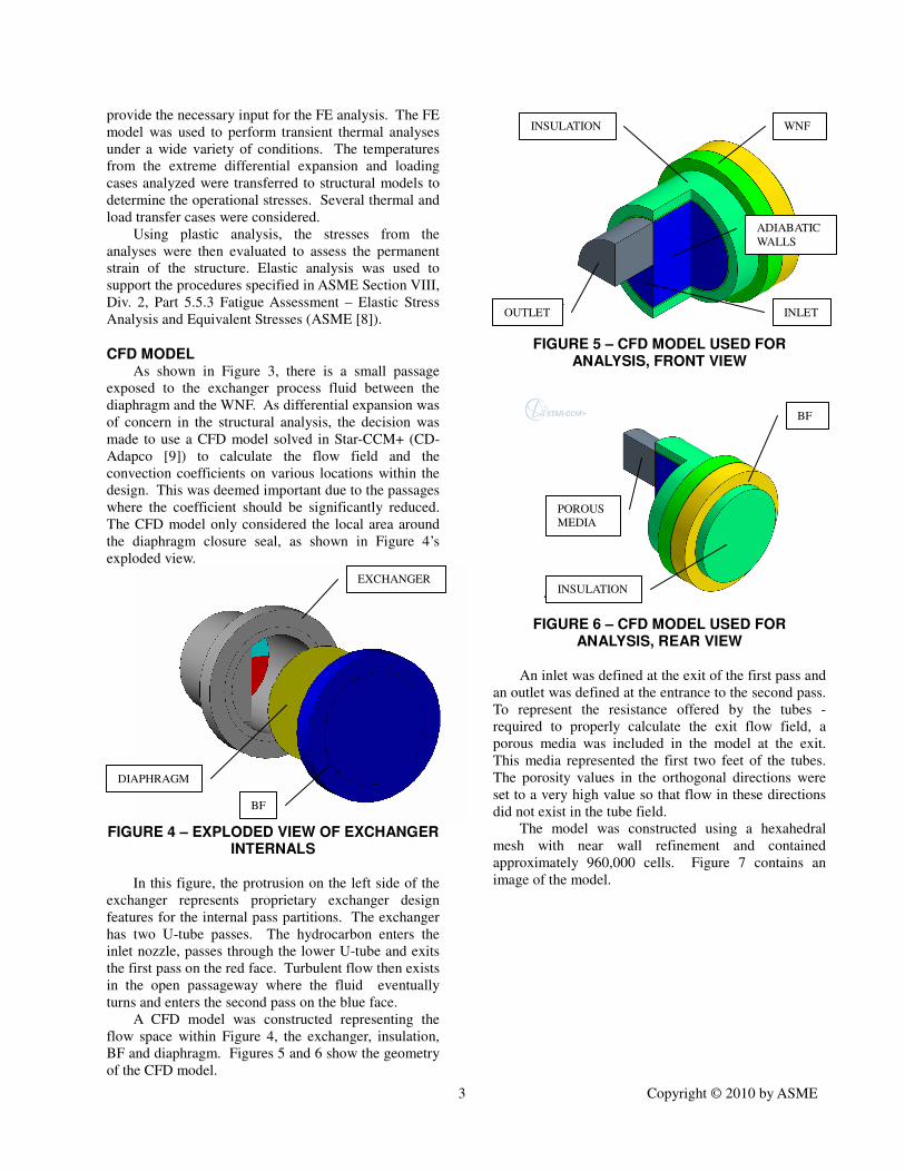
A CFD model was constructed representing the

flow space within Figure 4, the exchanger, insulation,

BF and diaphragm. Figures 5 and 6 show the geometry

of the CFD model.

FIGURE 5 – CFD MODEL USED FOR

ANALYSIS, FRONT VIEW

FIGURE 6 – CFD MODEL USED FOR

ANALYSIS, REAR VIEW

An inlet was defined at the exit of the first pass and

an outlet was defined at the entrance to the second pass.

To represent the resistance offered by the tubes -

required to properly calculate the exit flow field, a

porous media was included in the model at the exit.

This media represented the first two feet of the tubes.

The porosity values in the orthogonal directions were

set to a very high value so that flow in these directions

did not exist in the tube field.

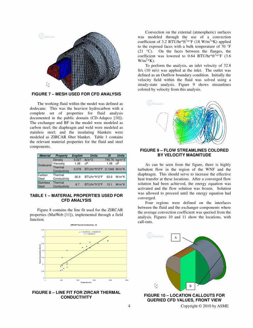
The model was constructed using a hexahedral

mesh with near wall refinement and contained

approximately 960,000 cells. Figure 7 contains an

image of the model.

DIAPHRAGM

EXCHANGER

BF

INSULATION

OUTLET

WNF

ADIABATIC

WALLS

INLET

BF

INSULATION

POROUS

MEDIA


FIGURE 7 – MESH USED FOR CFD ANALYSIS

The working fluid within the model was defined as

dodecane. This was the heaviest hydrocarbon with a

complete set of properties for fluid analysis

documented in the public domain (CD-Adapco [10]).

The exchanger and BF in the model were modeled as

carbon steel; the diaphragm and weld were modeled as

stainless steel; and the insulating blankets were

modeled as ZIRCAR fiber blanket. Table 1 contains

the relevant material properties for the fluid and steel

components.

Material Property English Units SI Units

Density 0.027 lb/in^3 745.76 kg/m^3

Viscosity 1.38 cP 1.38 cP

Thermal

Conductivity0.078 BTU/hr*ft^2*F 0.1349 W/m*K

Carbon

Steel

Thermal


Stainless

Steel

Thermal


Dodecane

TABLE 1 – MATERIAL PROPERTIES USED FOR CFD ANALYSIS

Figure 8 contains the line fit used for the ZIRCAR

properties (MatWeb [11]), implemented through a field

function.

ZIRCAR Thermal Conductivity - SI

y = 1.451559E-04x + 2.366236E-02

R2 = 7.830602E-01

0

0.05

0.1

0.15

0.2

0.25

0.3

0.35

0 500 1000 1500 2000 2500

Temperature (K)

Th

erm

al C

on

du

cti

vit

y (

W/m

*K)

FIGURE 8 – LINE FIT FOR ZIRCAR THERMAL CONDUCTIVITY

Convection on the external (atmospheric) surfaces

was modeled through the use of a convection

coefficient of 3.2 BTU/hr*ft2*°F (18 W/m

2*K) applied

to the exposed faces with a bulk temperature of 70 °F

(21 °C). On the faces between the flanges, the

coefficient was lowered to 0.64 BTU/hr*ft2*°F (3.6

W/m2*K).

To perform the analysis, an inlet velocity of 32.8

ft/s (10 m/s) was applied at the inlet. The outlet was

defined as an Outflow boundary condition. Initially the

velocity field within the fluid was solved using a

steady-state analysis. Figure 9 shows streamlines

colored by velocity from this analysis.

FIGURE 9 – FLOW STREAMLINES COLORED

BY VELOCITY MAGNITUDE

As can be seen from the figure, there is highly

turbulent flow in the region of the WNF and the

diaphragm. This should serve to increase the effective

heat transfer at these locations. After a converged flow

solution had been achieved, the energy equation was

activated and the flow solution was frozen. Solution

was allowed to proceed until the energy equation had

converged.

Four regions were defined on the interfaces

between the fluid and the exchanger components where

the average convection coefficient was queried from the

analysis. Figures 10 and 11 show the locations, with

call-outs.

FIGURE 10 – LOCATION CALLOUTS FOR QUERIED CFD VALUES, FRONT VIEW

A

B


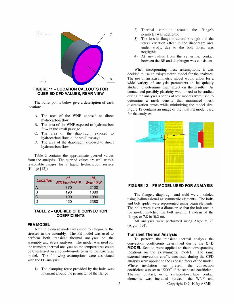
FIGURE 11 – LOCATION CALLOUTS FOR

QUERIED CFD VALUES, REAR VIEW

The bullet points below give a description of each

location:

A. The area of the WNF exposed to direct

hydrocarbon flow

B. The area of the WNF exposed to hydrocarbon

flow in the small passage

C. The area of the diaphragm exposed to

hydrocarbon flow in the small passage

D. The area of the diaphragm exposed to direct

hydrocarbon flow

Table 2 contains the approximate queried values

from the analysis. The queried values are well within

reasonable ranges for a liquid hydrocarbon service

(Hodge [12]).

Locationhi,

BTU/hr*ft^2*F

hi,

W/m^2*K

A 370 2100

B 190 1080

C 190 1080

D 420 2380

TABLE 2 – QUERIED CFD CONVECTION COEFFICIENTS

FEA MODEL A finite element model was used to categorize the

stresses in the assembly. The FE model was used to

perform both transient thermal analyses on the

assembly and stress analyses. The model was used for

the transient thermal analyses so the temperatures could

be transferred on a node–by-node basis to the structural

model. The following assumptions were associated

with the FE analysis:

1) The clamping force provided by the bolts was

invariant around the perimeter of the flange

2) Thermal variation around the flange’s

perimeter was negligible

3) The loss in flange structural strength and the

stress variation effect in the diaphragm area

under study, due to the bolt holes, was

negligible

4) At any radius from the centerline, contact

between the BF and diaphragm was consistent

When incorporating these assumptions, it was

decided to use an axisymmetric model for the analyses.

The use of an axisymmetric model would allow for a

wide variety of analysis parameters to be quickly

studied to determine their effect on the results. As

contact and possibly plasticity would need to be studied

during the analyses a series of test models were used to

determine a mesh density that minimized mesh

discretization errors while minimizing the model size.

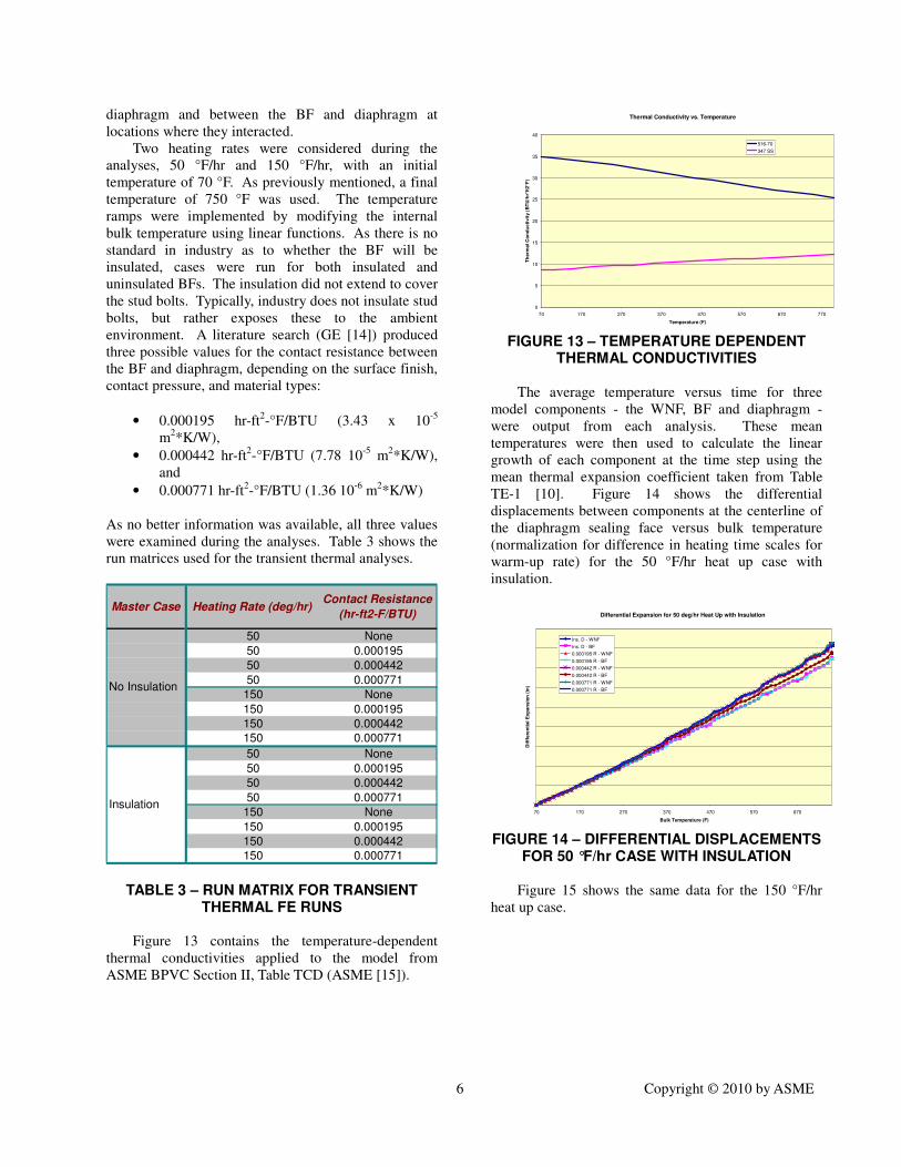
Figure 12 contains an image of the final FE model used

for the analyses.

FIGURE 12 – FE MODEL USED FOR ANALYSIS

The flanges, diaphragm and weld were modeled

using 2-dimensional axisymmetric elements. The bolts

and bolt spider were represented using beam elements.

The bolts were given a diameter so that the bolt area in

the model matched the bolt area in 1 radian of the

flange, or 7.8 in (0.2 m).

All analyses were performed using Algor v. 23

(Algor [13]).

Transient Thermal Analysis To perform the transient thermal analysis the

convection coefficients determined during the CFD MODEL Section were applied to their corresponding

locations on the axisymmetric model. The same

external convection coefficients used during the CFD

analysis were applied to the exposed faces of the model.

Where insulation was present, the convection

coefficient was set to 1/200th of the standard coefficient.

Thermal contact, using surface–to-surface contact

elements, was included between the WNF and

C

D


diaphragm and between the BF and diaphragm at

locations where they interacted.

Two heating rates were considered during the

analyses, 50 °F/hr and 150 °F/hr, with an initial

temperature of 70 °F. As previously mentioned, a final

temperature of 750 °F was used. The temperature

ramps were implemented by modifying the internal

bulk temperature using linear functions. As there is no

standard in industry as to whether the BF will be

insulated, cases were run for both insulated and

uninsulated BFs. The insulation did not extend to cover

the stud bolts. Typically, industry does not insulate stud

bolts, but rather exposes these to the ambient

environment. A literature search (GE [14]) produced

three possible values for the contact resistance between

the BF and diaphragm, depending on the surface finish,

contact pressure, and material types:

• 0.000195 hr-ft2-°F/BTU (3.43 x 10

-5

m2*K/W),

• 0.000442 hr-ft2-°F/BTU (7.78 10

-5 m

2*K/W),

and

• 0.000771 hr-ft2-°F/BTU (1.36 10

-6 m

2*K/W)

As no better information was available, all three values

were examined during the analyses. Table 3 shows the

run matrices used for the transient thermal analyses.

Master Case Heating Rate (deg/hr)Contact Resistance

(hr-ft2-F/BTU)

50 None

50 0.000195

50 0.000442

50 0.000771

150 None

150 0.000195

150 0.000442

150 0.000771

50 None

50 0.000195

50 0.000442

50 0.000771

150 None

150 0.000195

150 0.000442

150 0.000771

No Insulation

Insulation

TABLE 3 – RUN MATRIX FOR TRANSIENT THERMAL FE RUNS

Figure 13 contains the temperature-dependent

thermal conductivities applied to the model from

ASME BPVC Section II, Table TCD (ASME [15]).

Thermal Conductivity vs. Temperature

0

5

10

15

20

25

30

35

40

70 170 270 370 470 570 670 770

Temperature (F)

Th

erm

al C

on

du

cti

vit

y (

BT

U/h

r*ft

2*F

)

516-70

347 SS

FIGURE 13 – TEMPERATURE DEPENDENT

THERMAL CONDUCTIVITIES

The average temperature versus time for three

model components - the WNF, BF and diaphragm -

were output from each analysis. These mean

temperatures were then used to calculate the linear

growth of each component at the time step using the

mean thermal expansion coefficient taken from Table

TE-1 [10]. Figure 14 shows the differential

displacements between components at the centerline of

the diaphragm sealing face versus bulk temperature

(normalization for difference in heating time scales for

warm-up rate) for the 50 °F/hr heat up case with

insulation.

Differential Expansion for 50 deg/hr Heat Up with Insulation

70 170 270 370 470 570 670

Bulk Temperature (F)

Dif

ffere

nti

al

Exp

an

sio

n (

in)

Ins. D - WNF

Ins. D - BF

0.000195 R - WNF

0.000195 R - BF

0.000442 R - WNF

0.000442 R - BF

0.000771 R - WNF

0.000771 R - BF

FIGURE 14 – DIFFERENTIAL DISPLACEMENTS

FOR 50 °F/hr CASE WITH INSULATION

Figure 15 shows the same data for the 150 °F/hr

heat up case.


Differential Expansion for 150 deg/hr Heat Up with Insulation

70 170 270 370 470 570 670


Dif

fere

nti

al D

isp

lac

em

en

t (i

n)

WNF

BF

0.000195 R - WNF

0.000195 R - BF

0.000442 R - WNF

0.000442 R - BF

0.000771 R - WNF

0.000771 R - BF


FOR 150 °F/hr CASE WITH INSULATION

Figure 16 shows the differential displacements

between components for the 50 °F/hr heat up case

without insulation.

Differential Expansion for 50 deg/hr Heat Up without Insulation

70 170 270 370 470 570 670


Dif

fere

nti

al

Dis

pla

cem

en

ts (

in)

WNF

BF

0.000195 R - WNF

0.000195 R - BF

0.000442 R - WNF

0.000442 R - BF

0.000771 R - WNF

0.000771 R - BF


FOR 50 °F/hr CASE WITHOUT INSULATION

Figure 17 shows the same data for the 150 °F/hr

heat up case.

Differential Expansion for 150 deg/hr Heat Up without Insulation

70 170 270 370 470 570 670


Dif

fere

nti

al

Dis

pla

cem

en

ts (

in)

WNF

BF

0.000195 R - WNF

0.000195 R - BF

0.000442 R - WNF

0.000442 R - BF

0.000771 R - WNF

0.000771 R - BF


FOR 150 °F /hr CASE WITHOUT INSULATION

A comparison of the figures shows that the

differential displacements only vary based on the

insulation boundary condition; the maximum values for

a given insulation state are identical for both heating

rates. Also evident from the graphs is the fact that the

differential displacements are higher for the uninsulated

case than for the insulated case. This result is expected,

as the BF should heat up slower and operate at a lower

temperature when uninsulated.

Figure 18 contains the temperature differentials

between the diaphragm and the WNF and BF versus the

bulk temperature for the cases analyzed without

insulation.

Differential Temperatures between Component and Diaphragm

with Heating Rate, No Insulation

0

50

100

150

200

250

300

70 170 270 370 470 570 670


Dif

fere

nti

al T

em

pera

ture

s (

F)

WNF, No Resistance, 150 /hr

BF, No Resistance, 150 /hr

WNF, No Resistance, 50 /hr

BF, No Resistance, 50 /hr

WNF, 0.000195 R, 150/hr

BF, 0.000195 R, 150 /hr

WNF, 0.000195 R, 50 /hr

BF, 0.000195 R, 50 /hr

WNF, 0.000442 R, 150 /hr

BF, 0.000442 R, 150 /hr

WNF, 0.000442 R, 50 /hr

BF, 0.000442 R, 50 /hr

WNF, 0.00071 R, 150 /hr

BF, 0.000771 R, 150 /hr

WNF, 0.000771 R, 50 /hr

BF, 0.000771 R, 50 /hr

FIGURE 18 – DIFFERENTIAL TEMPERATURES

FROM TRANSIENT THERMAL ANALYSES

As can be seen in the figure, the contact resistance

does not affect the temperature differential between the

WNF and diaphragm. Also evident in the figure is that

the temperature differential between the BF and

diaphragm follows three lines, corresponding to the

different thermal resistances. The 0.000195 hr-ft2-

°F/BTU resistance produced almost the same results as

no resistance. The fact that the differential curves are

almost identical at both heating rates indicates that

heating rate is not significant in the differential

temperatures and corresponding strains within the

design. Therefore, it can be stated that the maximum

differential thermal strain will exist at the exchanger’s

operational temperature if a reasonable heating rate is

maintained during start-up. Steps will be taken during

the structural analysis to confirm or deny this statement.

Elastic Structural Analysis The same axisymmetric model used for the thermal

analysis was used for the structural analyses. The

thermal contact, previously mentioned, was modified to

structural contact. As no public domain data could

provide a source for the expected friction coefficient

between the diaphragm and flanges (only a maximum

value was posited), several values were analyzed,

including: no friction, 0.2, 0.4 and 0.6 as the

coefficients of static friction. The surface contact type


was stick-slip, so no dynamic coefficient of friction was

considered. This aids tremendously in model

convergence, and with the magnitude of forces

occurring in the exchanger should not be an

unreasonable assumption.

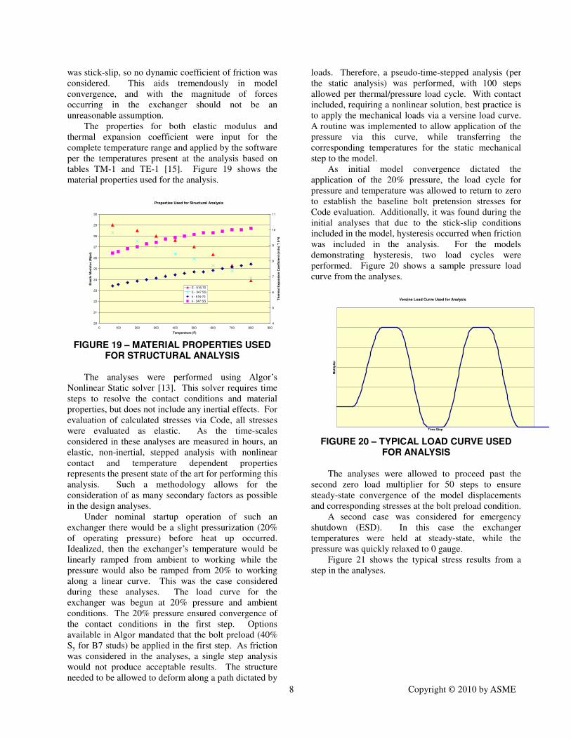
The properties for both elastic modulus and

thermal expansion coefficient were input for the

complete temperature range and applied by the software

per the temperatures present at the analysis based on

tables TM-1 and TE-1 [15]. Figure 19 shows the

material properties used for the analysis.

Properties Used for Structural Analysis

20

21

22

23

24

25

26

27

28

29

30

0 100 200 300 400 500 600 700 800 900

Temperature (F)

Ela

sti

c M

od

ulu

s (

Mp

si)

4

5

6

7

8

9

10

11

Th

erm

al

Exp

an

sio

n C

oe

ffic

ien

t (i

n/in

) *1

0^

6

E - 516-70

E - 347 SS

k - 516-70

k - 347 SS

FIGURE 19 – MATERIAL PROPERTIES USED

FOR STRUCTURAL ANALYSIS

The analyses were performed using Algor’s

Nonlinear Static solver [13]. This solver requires time

steps to resolve the contact conditions and material

properties, but does not include any inertial effects. For

evaluation of calculated stresses via Code, all stresses

were evaluated as elastic. As the time-scales

considered in these analyses are measured in hours, an

elastic, non-inertial, stepped analysis with nonlinear

contact and temperature dependent properties

represents the present state of the art for performing this

analysis. Such a methodology allows for the

consideration of as many secondary factors as possible

in the design analyses.

Under nominal startup operation of such an

exchanger there would be a slight pressurization (20%

of operating pressure) before heat up occurred.

Idealized, then the exchanger’s temperature would be

linearly ramped from ambient to working while the

pressure would also be ramped from 20% to working

along a linear curve. This was the case considered

during these analyses. The load curve for the

exchanger was begun at 20% pressure and ambient

conditions. The 20% pressure ensured convergence of

the contact conditions in the first step. Options

available in Algor mandated that the bolt preload (40%

Sy for B7 studs) be applied in the first step. As friction

was considered in the analyses, a single step analysis

would not produce acceptable results. The structure

needed to be allowed to deform along a path dictated by

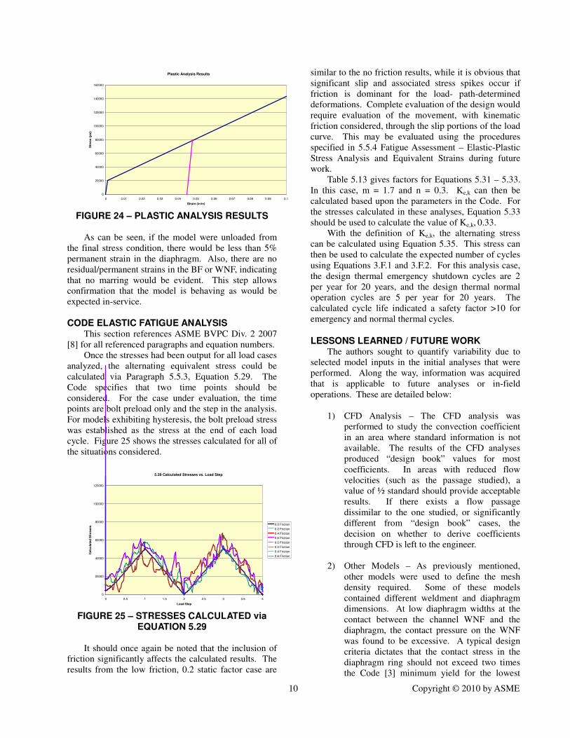
loads. Therefore, a pseudo-time-stepped analysis (per

the static analysis) was performed, with 100 steps

allowed per thermal/pressure load cycle. With contact

included, requiring a nonlinear solution, best practice is

to apply the mechanical loads via a versine load curve.

A routine was implemented to allow application of the

pressure via this curve, while transferring the

corresponding temperatures for the static mechanical

step to the model.

As initial model convergence dictated the

application of the 20% pressure, the load cycle for

pressure and temperature was allowed to return to zero

to establish the baseline bolt pretension stresses for

Code evaluation. Additionally, it was found during the

initial analyses that due to the stick-slip conditions

included in the model, hysteresis occurred when friction

was included in the analysis. For the models

demonstrating hysteresis, two load cycles were

performed. Figure 20 shows a sample pressure load

curve from the analyses.

Versine Load Curve Used for Analysis

Time Step

Mu

ltip

lier

FIGURE 20 – TYPICAL LOAD CURVE USED

FOR ANALYSIS

The analyses were allowed to proceed past the

second zero load multiplier for 50 steps to ensure

steady-state convergence of the model displacements

and corresponding stresses at the bolt preload condition.

A second case was considered for emergency

shutdown (ESD). In this case the exchanger

temperatures were held at steady-state, while the

pressure was quickly relaxed to 0 gauge.

Figure 21 shows the typical stress results from a

step in the analyses.


FIGURE 21 – TYPICAL STRESS RESULTS FROM ANALYSES

As can be seen from the figure, the peak stress in

the weld occurs at the weld–to-diaphragm OD location

and the peak stress in the diaphragm occurs at the

periphery where the diaphragm contacts the BF.

Therefore, step dependent stresses, σxx, σyy, σzz and τyz

(τxy and τxz were 0 due to the axisymmetric assumption)

at these two locations were output for Code evaluation.

Figure 22 shows typical queried stress results from an

analysis.

Typical Stress Results from Analyses

-400000

-350000

-300000

-250000

-200000

-150000

-100000

0 0.5 1 1.5 2 2.5 3 3.5 4 4.5

Load Step

Str

ess (

psi)

Sxx 0.0 Friction

Syy 0.0 Friction

Szz 0.0 Friction

Tyz 0.0 Friction

Sxx 0.6 Friction

Syy 0.6 Friction

Szz 0.6 Friction

Txy 0.6 Friction

FIGURE 22 – QUERIED STRESS RESULTS

FROM ANALYSIS

Assuming the use of 40% of stud minimum yield

as the original stud bolt up stress, the linear analysis

confirmed that the maximum stud stress did not exceed

yield during the thermal cycles analyzed. The 40% of

yield bolt up stress in the studs is considered to be

sufficient to meet a design for resisting the hydraulic

end force during hydrotest while maintaining at least

50% of the Code [6] minimum gasket seating stress.

The stresses indicated in the diaphragm and

associated weld exceed the allowable stress values;

therefore, an elastic fatigue analysis is required. The

procedures used in this analysis are detailed in the

CODE ELASTIC FATIGUE ANALYSIS Section.

Figure 23 shows the von Mises stress results from

the analyses as reported by Algor.

von Mises Stress vs. Load Step

0

50000

100000

150000

200000

250000

300000

350000

0 0.5 1 1.5 2 2.5 3 3.5 4

Load Step

Str

ess (

psi) 0.0 Friction

0.2 Friction

0.4 Friction

0.6 Friction

Start Load

Cycle

End Load Cycle,

Begin Cycle

Down

End Cycle

Down, Begin

Cycle Up

End Load Cycle,

Begin Second

Cycle Down

Termination

FIGURE 23 – von MISES STRESS RESULTS

FROM ANALYSES

As can be seen in the figure, significant hysteresis

exists in the system when friction is included. The

structure does not return to its preload state.

Accommodations for this fact will need to be taken

during the 5.5.4 Fatigue Assessment – Elastic-Plastic

Stress Analysis and Equivalent Strains Code stress

evaluation. As discussed in the FUTURE WORK

Section, additional analyses will need to be performed

to quantify the frictional effects.

Plastic Analysis Results To confirm the elastic analysis results, it was

decided to perform a plastic analysis on the structure.

Similar designs have been operated, maintained and

inspected over a 20+ year life cycle. From the authors’

experience, one would expect no gross deformation

(scarring) on the WNF and that plastic strains in the

diaphragm should be minimal ( < 5%).

To perform the analyses, temperature-dependent

yield strengths were defined for the materials [15]. The

strain hardening modulus above yield was defined as

5% of the elastic modulus. While this is typically high

for most materials, it allows for qualification of the

stress results without relying on proprietary

information, and also aids convergence.

The model was analyzed with a friction coefficient

of 0.6 through the previously described load curves.

Querying the maximum von Mises stress results at the

preload point in the load curve produces a value of ~80

ksi. Von Mises stress should be used for the queried

stresses, as these stresses are used for Algor’s yield

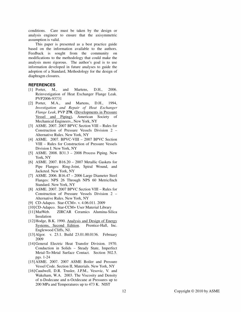
criteria. Figure 24 contains the results from the plastic

analysis.


Plastic Analysis Results

0

20000

40000

60000

80000

100000

120000

140000

160000

0 0.01 0.02 0.03 0.04 0.05 0.06 0.07 0.08 0.09 0.1

Strain (in/in)

Str

ess (

psi)

FIGURE 24 – PLASTIC ANALYSIS RESULTS

As can be seen, if the model were unloaded from

the final stress condition, there would be less than 5%

permanent strain in the diaphragm. Also, there are no

residual/permanent strains in the BF or WNF, indicating

that no marring would be evident. This step allows

confirmation that the model is behaving as would be

expected in-service.

CODE ELASTIC FATIGUE ANALYSIS This section references ASME BVPC Div. 2 2007

[8] for all referenced paragraphs and equation numbers.

Once the stresses had been output for all load cases

analyzed, the alternating equivalent stress could be

calculated via Paragraph 5.5.3, Equation 5.29. The

Code specifies that two time points should be

considered. For the case under evaluation, the time

points are bolt preload only and the step in the analysis.

For models exhibiting hysteresis, the bolt preload stress

was established as the stress at the end of each load

cycle. Figure 25 shows the stresses calculated for all of

the situations considered.

5.29 Calculated Stresses vs. Load Step

0

20000

40000

60000

80000

100000

120000

0 0.5 1 1.5 2 2.5 3 3.5 4

Load Step

Calc

ula

ted

Str

esses

0.0 Friction

0.2 Friction

0.4 Friction

0.6 Friction

0.0 Friction

0.2 Friction

0.4 Friction

0.6 Friction

FIGURE 25 – STRESSES CALCULATED via

EQUATION 5.29

It should once again be noted that the inclusion of

friction significantly affects the calculated results. The

results from the low friction, 0.2 static factor case are

similar to the no friction results, while it is obvious that

significant slip and associated stress spikes occur if

friction is dominant for the load- path-determined

deformations. Complete evaluation of the design would

require evaluation of the movement, with kinematic

friction considered, through the slip portions of the load

curve. This may be evaluated using the procedures

specified in 5.5.4 Fatigue Assessment – Elastic-Plastic

Stress Analysis and Equivalent Strains during future

work.

Table 5.13 gives factors for Equations 5.31 – 5.33.

In this case, m = 1.7 and n = 0.3. Ke,k can then be

calculated based upon the parameters in the Code. For

the stresses calculated in these analyses, Equation 5.33

should be used to calculate the value of Ke,k, 0.33.

With the definition of Ke,k, the alternating stress

can be calculated using Equation 5.35. This stress can

then be used to calculate the expected number of cycles

using Equations 3.F.1 and 3.F.2. For this analysis case,

the design thermal emergency shutdown cycles are 2

per year for 20 years, and the design thermal normal

operation cycles are 5 per year for 20 years. The

calculated cycle life indicated a safety factor >10 for

emergency and normal thermal cycles.

LESSONS LEARNED / FUTURE WORK The authors sought to quantify variability due to

selected model inputs in the initial analyses that were

performed. Along the way, information was acquired

that is applicable to future analyses or in-field

operations. These are detailed below:

1) CFD Analysis – The CFD analysis was

performed to study the convection coefficient

in an area where standard information is not

available. The results of the CFD analyses

produced “design book” values for most

coefficients. In areas with reduced flow

velocities (such as the passage studied), a

value of ½ standard should provide acceptable

results. If there exists a flow passage

dissimilar to the one studied, or significantly

different from “design book” cases, the

decision on whether to derive coefficients

through CFD is left to the engineer.

2) Other Models – As previously mentioned,

other models were used to define the mesh

density required. Some of these models

contained different weldment and diaphragm

dimensions. At low diaphragm widths at the

contact between the channel WNF and the

diaphragm, the contact pressure on the WNF

was found to be excessive. A typical design

criteria dictates that the contact stress in the

diaphragm ring should not exceed two times

the Code [3] minimum yield for the lowest


yield material during hydrotest and normal

operation. The authors intend to explore this

issue further in the future.

3) Insulation – From the results presented in this

paper, it is obvious that a BF with insulation

does not cause as much differential expansion

as a BF without insulation. If an operator

believes that a closure (such as studied in this

paper) may be subjected to excessive

differential expansion conditions, the addition

of an insulating blanket on the blind flange not

extending to the stud bolts will reduce

operating differential expansion and stresses.

4) Material Properties – As mentioned in the

paper, at the time of the analyses very limited

public domain data was available for the

hydrocarbon fluid properties. Since that time,

the authors have found a public domain source

for dodecane fluid properties as a function of

temperature and pressure (Caudwell [16]).

While the fluid properties are very similar to

the properties used in these analyses, they

allow for a more rigorous CFD analysis to be

performed. The authors desire to implement

these properties into the CFD model to ensure

that the calculated coefficients are valid over

the entire cycle range. It is expected that the

CFD results will not be significantly affected,

as the calculated results were similar to

standard heat transfer coefficients. If the

authors find that significant variation occurs

with the complete properties, the results will

be reported to the community.

5) Friction – As discussed in the FEA MODEL

section, the stick-slip assumption is considered

to be valid. Time was not available to test

complete friction modeling with inertia.

Investigation of this may be considered for

additional justification in the use of the stick-

slip assumption. Additionally, due to the

highly nonlinear nature of this process, it

would be wise to verify results though the use

of at least 2 FE analysis codes. The authors

intend to perform this verification.

6) Cycle Count – It is obvious from the results

that the model - including friction - is highly

nonlinear in response. While the procedures

detailed above chose an arbitrary preload state

for Code calculations, it is advised that

numerous cycles (10+) should be considered in

the analysis. Per Code, the baseline, pre-stress

state would need to be established and a cycle

count would need to be performed for each of

the cycles exhibiting hysteresis. Ideally, many

analysis cycles run on the frictional models

would result in a determinant result for the bolt

preload stress case. This stress could then be

used to establish operational alternating

stresses due to thermal cycles. The authors

intend to perform this analysis.

7) Additional Analysis – While the models

presented in this paper were adequate to

capture the behaviors needed for Code

evaluation, they were not refined enough to

capture gross deformation at the highly

stressed weld location and at the contact

between the diaphragm and the BF. All

requirements for evaluation via Paragraph

5.5.2, Equation 5.29 were met. It is the

authors’ intention to also perform evaluation

via Equation 5.25 through the implementation

of additional load cases. The authors also

intend to refine the model and perform Code

evaluations as defined in Paragraph 5.5.4,

Fatigue Assessment – Elastic-Plastic Stress

Analysis and Equivalent Strains to compare to

the elastic fatigue results obtained by the

procedures reported in this paper. Results will

be published to aid in guiding design

methodology decisions.

CONCLUSIONS A procedure including reasonable analysis

methodology has been demonstrated for the evaluation

of a diaphragm closure. In this instance, for the load

cases considered, the diaphragm closure should meet

the number of cycles that typically occur in a plant.

This analysis result has been confirmed through long-

term operation of similar closures.

It should be noted that the authors have only

considered two plant operating cases, normal thermal

cycle and ESD. In Assessment Procedure 5.5.3.2, Step

1, it is specified that all load histories should be

established. Therefore, this paper should not be used as

a reference for establishing the complete design

suitability of a certain closure. That said, the

procedures established in this paper can be used to

qualify a specific load history when established, as well

as the resulting differential thermal expansion and

stress.

It should be noted, as detailed above, that several

important assumptions were made in the analyses

presented. When any of the assumptions are violated,

the procedures specified in this paper may not be valid.

Specifically, in the previous paper [1] steps were not

taken in the design to minimize thermal variations. It

should be noted that in the design considered, steps

were taken to ensure that the diaphragm was exposed to

a nearly consistent temperature and fluid side process


conditions. Care must be taken by the design or

analysis engineer to ensure that the axisymmetric

assumption is valid.

This paper is presented as a best practice guide

based on the information available to the authors.

Feedback is sought from the community on

modifications to the methodology that could make the

analysis more rigorous. The author’s goal is to use

information developed in future analyses to guide the

adoption of a Standard, Methodology for the design of

diaphragm closures.

REFERENCES [1] Porter, M., and Martens, D.H., 2006.

Reinvestigation of Heat Exchanger Flange Leak.

PVP2006-93731

[2] Porter, M.A., and Martens, D.H., 1994,

Investigation and Repair of Heat Exchanger

Flange Leak, PVP 278, (Developments in Pressure

Vessel and Piping), American Society of

Mechanical Engineers., New York, NY

[3] ASME. 2007. 2007 BPVC Section VIII – Rules for

Construction of Pressure Vessels Division 2 –

Alternative Rules. New York, NY

[4] ASME. 2007. BPVC-VIII – 2007 BPVC Section

VIII – Rules for Construction of Pressure Vessels

Division I. New York, NY

[5] ASME. 2008. B31.3 – 2008 Process Piping. New

York, NY

[6] ASME. 2007. B16.20 – 2007 Metallic Gaskets for

Pipe Flanges: Ring-Joint, Spiral Wound, and

Jacketed. New York, NY

[7] ASME. 2006. B16.47 – 2006 Large Diameter Steel

Flanges: NPS 26 Through NPS 60 Metric/Inch

Standard. New York, NY

[8] ASME. 2007. 2007 BPVC Section VIII – Rules for

Construction of Pressure Vessels Division 2 –

Alternative Rules. New York, NY

[9] CD-Adapco. Star-CCM+. v. 4.06.011. 2009

[10] CD-Adapco. Star-CCM+ User Material Library

[11] MatWeb. ZIRCAR Ceramics Alumina-Silica

Insulation

[12] Hodge, B.K. 1990. Analysis and Design of Energy

Systems, Second Edition. Prentice-Hall, Inc.

Englewood Cliffs, NJ.

[13] Algor. v. 23.1. Build 23.01.00.0136. February

2009

[14] General Electric Heat Transfer Division. 1970.

Conduction in Solids – Steady State, Imperfect

Metal-To-Metal Surface Contact. Section 502.5.

pgs. 1-24

[15] ASME. 2007. 2007 ASME Boiler and Pressure

Vessel Code. Section II, Materials. New York, NY

[16] Caudwell, D.R. Trusler, J.P.M., Vesovic, V. and

Wakeham, W.A. 2003. The Viscosity and Density

of n-Dodecane and n-Octdecane at Pressures up to

200 MPa and Temperatures up to 473 K. NIST

Documents

2010 PV -25883 4 21 2 - Home - Porter McGuffie, Incpm-engr.com/wp-content/uploads/2015/10/PVP2010_25… · · 2017-06-02Proceedings of the ASME 2010 Pressure Vessels & Piping Division