2009-05-14 Neil Campbell Paper ANZSASI 2009

5/10/2018 2009-05-14 Neil Campbell Paper ANZSASI 2009 - slidepdf.com

http://slidepdf.com/reader/full/2009-05-14-neil-campbell-paper-anzsasi-2009 1/17

Evaluating Computer Graphics Animations

of Aircraft Accidents and Incidents

Neil A. H. Campbell MO3806

Neil graduated in 1983, with a Bachelor of Engineering degree (Electronics), from theUniversity of Western Australia. In 1986 he joined the Bureau of Air Safety Investigation as a flight recorder specialist. Neil took a leave of absence during 1994-1995 and managed the flight data analysis program for Gulf Air in Bahrain. During 1998 he was a member of the ICAO Flight Recorder Panel that developed changes toICAO Annex 6. In February 2000, Neil joined the Corporate Safety Department of Cathay Pacific Airways Limited in Hong Kong. During 2001 and 2002 he held the position of Manager Air Safety. In December 2003 he rejoined the Australian Transport Safety Bureau as a Senior Transport Safety Investigator.

CONTENTS

1. Introduction

2. History Of Computer Graphics Animations

3. Current Animation Software

4. Characteristics Of Digital Data

4.1 Sampling Rates4.2 Interpolation

4.3 Smoothing

4.4 Clamping

4.5 ARINC 429 Digital Information Transfer System (DITS) Cycling

4.6 Conversion Of Raw FDR Data To Engineering Units

5. Ground Track Generation

6. Satellite Imagery And Terrain Databases

7. Checklist For Evaluating An Animation

8. Conclusion



1. INTRODUCTION

Computer graphics animations of aircraft accidents and incidents are now widely available and

viewed. Animations can show a 3-dimensional view of an aircraft from any vantage point, an

aircraft flight path, cockpit instrument panels, pilot control inputs and aircraft control surface

deflections. Many different organisations and individuals can produce animations for a variety

of purposes:

• news organisations

• animation software developers/users

• airlines

• aircraft manufacturers

• aviation regulators

• government air safety investigators

• parties involved in litigation

Animations can be useful as they:

• help to assimilate large amounts of data

• place a sequence of events into time perspective

• link recorded data with ground features

• correlate flight data recorder (FDR) data with other sources of data e.g. cockpit voice

recorder (CVR) audio, radar data or eyewitness statements

• provide a useful analysis tool for investigators

• aid explanation of an event to lay persons

• provide a training/educational tool

Animations can be misleading as they may:

• present data in a biased way – highlighting a particular aspect of the data

• fill gaps in factual data with incorrect values

• have been produced using incorrect assumptions

• show misleading weather, visibility or lighting conditions

2



2. HISTORY OF COMPUTER GRAPHICS ANIMATIONS

In 1980 it was proposed1 that the Air Safety Investigation Branch2 develop a computer graphics

system. In 1984, the Bureau of Air Safety Investigation (BASI) introduced its first computer

graphics system which made BASI one of the first government accident investigation

authorities to use this technology. The system comprised an Evans and Sutherland PS300

monochrome vector graphics workstation hosted by a PDP 11/45 mini-computer. This systemcould animate a simulated instrument panel, an instrument landing system (ILS) approach as

well as a general 3-dimensional view. The accident to VH-IWJ, in 1985, was the first accident

in Australia to be investigated using this technology.

In the 1980’s the hardware required to perform animations was expensive and only accessible to

organisations with large budgets. The animations produced were constrained by the small

number of FDR parameters available and computer hardware constraints limiting the amount of

terrain data that could be displayed. They did not pretend to be realistic and ‘seeing was

definitely not believing’.

Figure 1: Animation (1986) showing a 3-d view of the aircraft and coastline.

Nowadays, a modern home personal computer or laptop is capable of performing animations.

Thousands of FDR parameters are available as well as satellite terrain imagery. Animations can

be very realistic and ‘seeing is believing’.

More than ever, it is important to critically evaluate animations before relying on them as

important evidence.

1 Recorder Research Note 12, P. Mayes, Air Safety Investigation Branch, December 1980.2 In 1982, the Air Safety Investigation Branch (ASIB) was re-organised to become the Bureau of Air Safety

Investigation (BASI). On 1 July 1999, the multi-modal Australian Transport Safety Bureau was created by

combining BASI with other agencies.

3



Figure 2: Animation (2006) showing a 3-d view of the aircraft and instrument panel .3

3 The investigation report, including a download of the animation, is available at:

http://www.atsb.gov.au/publications/investigation_reports/2005/AAIR/aair200503722.aspx

4





3. CURRENT ANIMATION SOFTWARE

Many software packages are now available to create animations or to perform simulations.4

The ATSB uses Flightscape’s Insight® suite of software for flight data recovery, analysis and

animation. It is an open-architecture and integrated system so that data transfer from initial

recovery, data analysis (data listings and plots) and animation is seamless. The ATSB also usesTeledyne’s Ground Replay and Analysis Facility (GRAF) software to easily access and analyse

airline quick access recorder (QAR) data.

However, best-practice animations do not require any particular software and many different

software packages could be used if enough care is taken and enough expertise is available by

the user.

This is a partial list of current animation/simulation software:

Insight® animation Flight data animator

http://www.flightscape.com/products/animation.php

AirFASE® Flight data animator

teledynecontrols.com/pdf/AirFASE_Brochure.pdf

FlightViz™ Flight data animator

http://www.qinetiq-na.com/products-3d-graphicsal-visualization-flt-vis.htm

CEFA Flight data animator

http://www.cefa-aviation.com/flight_data_animation.htm

AGS Flight data animator

http://www.sagem-ds.com/ags/en/site.php?spage=02000000

X-Plane® Flight simulator

http://www.x-plane.com/about.html

xwave’s Flight animation system

http://www.xwavesolutions.com/files/credentials/ flight _ animation _system.pdf

FlightGear Flight simulator

http://www.flightgear.org/introduction.html

Microsoft® Flight Simulator

http://www.microsoft.com/games/flightsimulatorX/

4

A simulation predicts how an aircraft should behave given its initial conditions, control inputs and a knowledgeof the aircraft stability and control equations. The predicted behaviour can then be compared with the actual

behaviour recorded by the FDR. Any differences could be due to external factors such as meteorological effects

or aircraft malfunctions. In practice, only the aircraft manufacturer will have access to the complete

mathematical models required for simulations and accident investigation authorities often work cooperatively

with the manufacturer to obtain a simulation.

5


http://opt/scribd/conversion/tmp/scratch15005/teledynecontrols.com/pdf/AirFASE_Brochure.pdf





http://www.xwavesolutions.com/files/credentials/flight_animation_system.pdf




http://opt/scribd/conversion/tmp/scratch15005/teledynecontrols.com/pdf/AirFASE_Brochure.pdf





http://www.xwavesolutions.com/files/credentials/flight_animation_system.pdf





4. CHARACTERISTICS OF DIGITAL FDR DATA

4.1 Sampling Rates

The nature of digital data means that a continuous physical quantity, e.g. static pressure,

is periodically sampled and converted to a number. The continuous record of the

physical quantity is not available only the sampled values. If the system is well-designedthen the sampling rate will be high enough to avoid any loss of significant data. Typical

sampling rates of onboard avionics can be 100 or more times a second but the sampling

rates used by FDR’s and QAR’s are much lower typically ranging between 8 times per

second (e.g. vertical acceleration) to once every 64 seconds (e.g. fuel quantity).

To give the illusion of smooth motion, a computer graphics animation will use a frame

rate of 20 frames or more per second. The issue, for animations derived from FDR data,

is how to produce the extra values required to fill the gaps between the recorded

samples.

Figure 3: The flow of data from a sensor, e.g. Air Data Inertial Reference Unit (ADIRU), to theFDR to being recovered from the FDR and being processed by analysis software, to finally being

displayed in an animation.

The options ‘to fill the gaps’ include:

• retaining the value of the previous sample until the next value is recorded

• linearly interpolating between two samples

• smoothing between a number of samples

• using systems knowledge to infer values between samples

There is no consistently correct technique. For some parameters it is reasonable to

linearly interpolate between samples and for others it is reasonable to smooth betweensamples.

6



4.2 Interpolation

If an aircraft is in cruise at 36,000 ft and a series of altitude values of 36,000 ft are

recorded one second apart then, given the inertia of the aircraft, it is reasonable to

assume that the altitude was 36,000 ft in between the samples.

In other cases it is not reasonable to interpolate between samples. Figures 4 & 5 are FDR

plots showing which FCPC5 was operating as the master FCPC. Figure 4 apparently

shows that initially FCPC 1 was master, then FCPC 2 became master and later FCPC 1

again became master. A line is drawn on the plot (interpolating) between the parameter

values which were sampled four seconds apart.

The aircraft manufacturer advised that a FCPC fault indication cannot occur unless the

relevant FCPC was master at the time of the fault indication. Applying this knowledge

of the flight control system, Figure 5 shows that initially FCPC 1 was master, then

FCPC 3 became master and then FCPC 2 became master.

If the data was not carefully analysed before being animated then it would display

incorrect information. Given that an animation may use hundreds of parameters, this

example shows the need for careful analysis of the data before presenting an animation

‘as what really happened’.

Figure 4: An FDR plot showing which FCPC was master.

5 Some Airbus aircraft have three Flight Control Primary Computers (FCPC’s). Only one at a time is master, the

other two are backups.

7



Figure 5: An expanded FDR plot showing which FCPC was master.

4.3 Smoothing

Figure 6 shows an aircraft ground track derived from latitude and longitude data

recorded by an FDR. The flight data acquisition unit, which sends data to the FDR, was

programmed to send 16 data bits for latitude and 16 bits for longitude. This equates to a

resolution of 180 deg x 60 NM/deg x 1852 metres/NM x 1/216 bits = 305.2 metres/bit.

If the aircraft had a ground speed of 200 kts (102.9 metres/sec), then if it was flying

North/South it would take approximately 3 seconds before it had travelled far enough to

result in a change to the recorded latitude. As latitude and longitude were each recorded

every second, this lack of resolution resulted in the stepping seen in the aircraft ground

track shown in the upper image of Figure 6. As the aircraft (a B737) was in controlled

flight during this period and, given its inertia, it was reasonable to smooth the recorded

ground track (refer to the lower image of Figure 6). In fact, it would be unreasonable to

have left the ground track unsmoothed.

8



Figure 6: Plots of latitude and longitude, upper image (as recorded) and lower image (smoothed).

9



4.4 Clamping

Figure 7 shows an example of a parameter being clamped at a fixed value. The exhaust

gas temperature (EGT) for the left engine increased to 1,149 °C and remained clamped

at this value for one minute and 46 seconds before decreasing. This behaviour was

unrealistic and the actual EGT would have been above 1,149 °C during the period it wasclamped.

The clamping value may have been determined by the flight data acquisition unit and the

value displayed on the pilot’s display may not have been clamped. Simply animating

this data and displaying it on an instrument panel ‘as what the pilot would have seen’

could be misleading.

Figure 7: An FDR plot showing a clamped parameter (EGT for the left engine).

10



4.5 ARINC 429 Digital Information Transfer System (DITS) Cycling

Digital avionics requires a system to transfer data between units. A widely used system

is the ARINC 429 Digital Information Transfer System (DITS). An ARINC 429 word

consists of 32 bits and for a binary parameter these include 19 bits for data and 3 bits for

a Sign/Status Matrix (SSM). The SSM is used to indicate the following conditions:

• failure warning

• no computed data

• functional test

• normal operation

Other aircraft systems can then accept or ignore parameter data depending on the SSM.

Only the data part of an ARINC 429 word is normally recorded by an FDR, not the

SSM. To indicate when non-normal data is being sent to the FDR, some flight data

acquisition units (FDAU’s) will insert a repetitive word pattern6, or cycling, into the

FDR data stream. An example is shown in Figure 8 where angle of attack (AOA) and

computed airspeed (CAS) parameters indicate ‘no computed data’ until there is

sufficient airflow for the AOA vane and pitot tube respectively to provide reasonable

values to the aircraft’s Air Data Inertial Reference Unit (ADIRU). Until that occurs, the

ADIRU will output, for these parameters, an SSM for ‘no computed data’. As a

consequence, the FDAU will output the cycling values to the FDR.

This cycling would not appear on the pilot’s display. Simply animating this data and

displaying it on an instrument panel ‘as what the pilot would have seen’ would be

misleading.

Figure 8: FDR plot during takeoff showing DITS cycling for AOA and CAS.

6 For example the pattern for no computed data is typically “data, 4000 octal, data, 0” which is repeated every four

seconds.

11



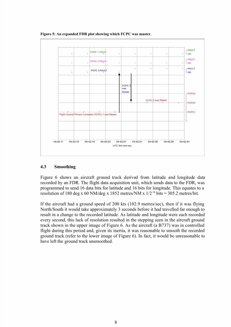
4.6 Conversion of raw FDR data to engineering units

Figure 9 shows the data flow through an FDR system. An essential step in data recovery

is the engineering units conversion where the raw binary data is mathematically

processed to obtain the relevant engineering unit e.g. the raw data recorded for indicated

airspeed is converted to knots. For modern airliners, recording hundreds or thousands of parameters, it is a huge task to obtain accurate system documentation, develop the

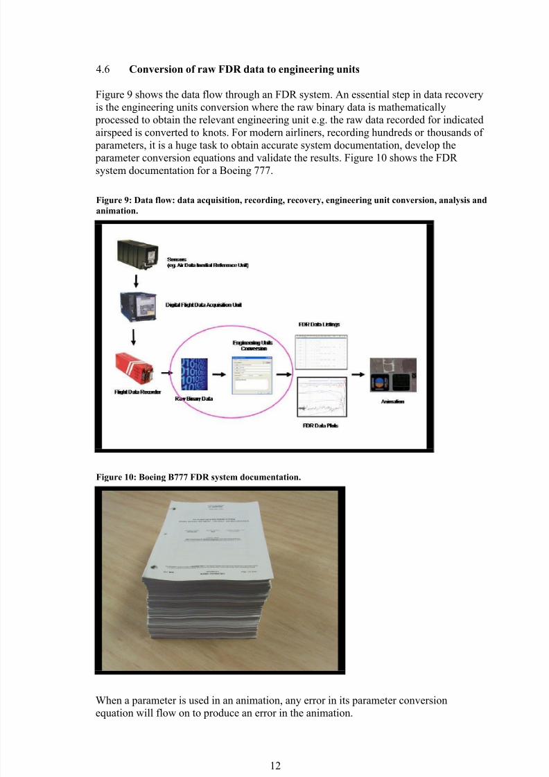
parameter conversion equations and validate the results. Figure 10 shows the FDR

system documentation for a Boeing 777.

Figure 9: Data flow: data acquisition, recording, recovery, engineering unit conversion, analysis and

animation.

Figure 10: Boeing B777 FDR system documentation.

When a parameter is used in an animation, any error in its parameter conversion

equation will flow on to produce an error in the animation.

12



5. GROUND TRACK GENERATION

Many different FDR parameters and techniques can be used to generate an aircraft ground

track. Table 1 summarises the most commonly used:

Figure 11: An example of residual groundspeed values at the gate after landing.

Parameter source: Comments:

GPS latitude and longitude GPS is usually the most accurate source of

latitude and longitude data provided that enough

satellites were in view. Don’t assume absolute

accuracy - software errors are still possible in the

GPS receiver or in the FDR parameter

conversion software. If the ground track is

displayed with a terrain overlay, then correct

geo-referencing of any satellite imagery is vital.

FMC latitude and longitude FMC latitude and longitude are produced by

weighting all the IRS positions with updates

from radio navigation aid fixes.IRS latitude and longitude Uncorrected latitude and longitude from one of

the IRS’s. The latitude and longitude errors will

increase with time so that the recorded latitude

and longitude at landing may be off the runway.

Groundspeed, heading and drift A generally accurate technique but beware of

parameter accuracies e.g. residual groundspeed

(refer to Figure 11). A sensitivity analysis can

show realistic error bounds for the ground track

i.e. vary the parameters over their expected

accuracy range e.g. ± 5 kts for groundspeed, ± 2

degrees for drift etc.Airspeed, pressure altitude, heading,

estimated wind and estimated

temperature

The least accurate technique for determining the

ground track from FDR data. Airspeed, pressure

altitude and heading are recorded parameters but

wind speed, wind direction and temperature will

need to be estimated. As wind is a function of

both time and altitude it is difficult to estimate

accurately. A sensitivity analysis can show

realistic error bounds for the ground track i.e.

vary the parameters over their expected accuracy

range. Figure 12 shows the effects of a ± 5 kts

wind speed variation accumulating over a 28

minute period. The aircraft airspeed ranged

between 125 kts – 190 kts.

13



Figure 12: Variations in calculated ground track over a 28 minute period. The

difference in position at the end of this period is 4,300 metres. Errors accumulate

with time.

6. SATELLITE IMAGERY AND TERRAIN DATABASES

The Shuttle Radar Topography Mission (SRTM) was a joint project between the National

Geospatial-Intelligence Agency and the National Aeronautics and Space Administration. The

objective of this project was to produce digital terrain elevation data (DTED) for 80% of theEarth's land surface (all land areas between 60° north and 56° south latitude), with data points

located every 1-arc second (approximately 30 metres) on a latitude/longitude grid. The

absolute vertical accuracy of the elevation data is 16 metres (at 90% confidence). The mission

14

Time



was flown in February 2000 and the SRTM data is publicly available.7 The data publicly

available for Australia is 3-arc second (approximately 90 metre) resolution.

Combining digital terrain elevation data with topographic maps or images from Google Earth

can be highly effective when portraying aircraft tracks. Figure 13 gives an example using the

versatile but low-cost OziExplorer 8 application.

It is the responsibility of the person producing the animation to check that the geo-referencing

of maps, satellite imagery and terrain used in the animation is accurate.

Figure 13: An aircraft flight path obtained from Automatic Dependent Surveillance – Broadcast (ADS-B)

data.

7 Refer to http://seamless.usgs.gov/website/seamless/8 For more information: http://www.oziexplorer.com/

15

http://seamless.usgs.gov/website/seamless/


http://www.oziexplorer.com/






7. CHECKLIST FOR EVALUATING AN ANIMATION

7.1 □ Who and what organisation produced the animation?

Government investigation agency, aircraft manufacturer, airline, partyinvolved in litigation, news organisation etc

7.2 □ What was the purpose of the animation?

7.3 □ Is the animation clearly titled and attributed?

7.4 □ Is a report available documenting how the animation was produced?9

The report should detail all the assumptions and judgements that have been

required to generate the animation e.g. how has data been inserted between sampled values, which key parameters have been interpolated, clamped,

truncated, rounded, smoothed or otherwise manipulated?

7.5 □ Are the sources of data for the animation listed?

FDR, QAR, CVR, air traffic control audio, radar, system BITE (built in test equipment) e.g. data stored in enhanced ground proximity warning system10

(EGPWS) non-volatile memory, meteorological reports, eyewitnesses etc

7.6 □ How has data from different sources been synchronised?

e.g. How has audio been synchronised with flight data?

7.7 □ Is a time reference shown on the animation?

What is the source of the time information? Is the animation real-time? Is theanimation continuous or have periods been cut-out?

7.8 □ What weather, visibility and lighting conditions are shown in the

animation?

Weather, visibility and lighting conditions are not recorded by an FDR. How

has this information been determined and represented?

7.9 □ Have satellite imagery and terrain databases been used?

Has the geo-referencing of the imagery been checked e.g. using surveyed locations?

7.10 □ Has a runway model been used?

Is it the correct model? Have the dimensions been checked? Are the runway

lights correctly represented?

9 Refer to pages A-63 to A-65 of ATSB Report 200501977 for an example of an animation report.

http://www.atsb.gov.au/publications/investigation_reports/2005/AAIR/aair200501977.aspx10 Refer to http://asasi.org/papers/2005/Use%20of%20EGPWS.pdf for an example of EGPWS data usage.

16


http://asasi.org/papers/2005/Use%20of%20EGPWS.pdf







7.11 □ What aircraft model has been used?

Is it the correct model? Have the dimensions been checked?

8. CONCLUSION

Computer graphics animations of aircraft accidents and incidents are routinely produced by a

variety of organisations – the purpose of these animations is not always to present data

objectively.

The challenge for the animators of flight data is to ensure that flight data is validated, analysed

and presented objectively and accurately. There should be sufficient documentation for an

animation, like other scientific results, to be reproducible.

The challenge for the viewers of animations is to critically evaluate what they are seeing, before

relying on it as important evidence.

17

Documents

2009-05-14 Neil Campbell Paper ANZSASI 2009