Embed Size (px)
Citation preview
2008 Load Impact Evaluation of California Statewide Aggregator Demand Response
Programs
Volume 1 : Ex Post and Ex Ante Report
CALMAC Study ID PGE0274.01
Steven D. Braithwait, Daniel G. Hansen, and
David Armstrong
Christensen Associates Energy Consulting, LLC
4610 University Ave., Suite 700 Madison, WI 53705
(608) 231-2266
May 1, 2009

Acknowledgements
We would like to thank several members of the Demand Response Monitoring and Evaluation Committee for their support in this project, including Gil Wong of PG&E, Kathryn Smith and Leslie Willoughby of SDG&E, Ed Lovelace of SCE, and Bruce Perlstein of Strategy, Finance & Economics, LLC.
CA Energy Consulting i
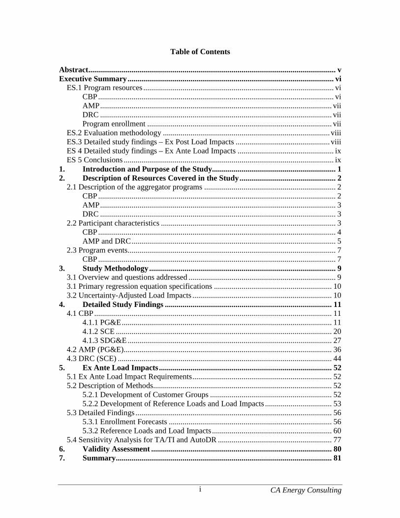
Table of Contents
Abstract.............................................................................................................................. v Executive Summary......................................................................................................... vi
ES.1 Program resources ................................................................................................. vi CBP........................................................................................................................ vi AMP...................................................................................................................... vii DRC ...................................................................................................................... vii Program enrollment .............................................................................................. vii
ES.2 Evaluation methodology ..................................................................................... viii ES.3 Detailed study findings – Ex Post Load Impacts................................................ viii ES 4 Detailed study findings – Ex Ante Load Impacts................................................. ix ES 5 Conclusions ........................................................................................................... ix
1. Introduction and Purpose of the Study............................................................... 1 2. Description of Resources Covered in the Study................................................. 2
2.1 Description of the aggregator programs ................................................................... 2 CBP......................................................................................................................... 2 AMP........................................................................................................................ 3 DRC ........................................................................................................................ 3
2.2 Participant characteristics ......................................................................................... 3 CBP......................................................................................................................... 4 AMP and DRC........................................................................................................ 5
2.3 Program events.......................................................................................................... 7 CBP......................................................................................................................... 7
3. Study Methodology............................................................................................... 9 3.1 Overview and questions addressed ........................................................................... 9 3.1 Primary regression equation specifications ............................................................ 10 3.2 Uncertainty-Adjusted Load Impacts ....................................................................... 10
4. Detailed Study Findings ..................................................................................... 11 4.1 CBP......................................................................................................................... 11
4.1.1 PG&E........................................................................................................... 11 4.1.2 SCE .............................................................................................................. 20 4.1.3 SDG&E........................................................................................................ 27
4.2 AMP (PG&E).......................................................................................................... 36 4.3 DRC (SCE) ............................................................................................................. 44
5. Ex Ante Load Impacts........................................................................................ 52 5.1 Ex Ante Load Impact Requirements....................................................................... 52 5.2 Description of Methods........................................................................................... 52
5.2.1 Development of Customer Groups .............................................................. 52 5.2.2 Development of Reference Loads and Load Impacts .................................. 53
5.3 Detailed Findings .................................................................................................... 56 5.3.1 Enrollment Forecasts ................................................................................... 56 5.3.2 Reference Loads and Load Impacts............................................................. 60
5.4 Sensitivity Analysis for TA/TI and AutoDR .......................................................... 77 6. Validity Assessment ............................................................................................ 80 7. Summary.............................................................................................................. 81
Figures
FIGURE 4.1: HOURLY LOADS AND LOAD IMPACTS – PG&E CBP DO EVENT (JUNE 20)..............................................15 FIGURE 4.2: UNCERTAINTY-ADJUSTED LOAD IMPACTS – PG&E CBP DO EVENT (JUNE 20) ......................................15 FIGURE 4.3: HOURLY LOADS AND LOAD IMPACTS – PG&E CBP DA EVENT (AUGUST 14)..........................................18 FIGURE 4.4: UNCERTAINTY-ADJUSTED LOAD IMPACTS – PG&E CBP DA EVENT (AUGUST 14) ..................................18 FIGURE 4.5: PG&E TOTAL NOMINATED CBP LOAD, JUNE 20 EVENT..........................................................................19 FIGURE 4.6: PG&E TOTAL NOMINATED CBP LOAD, AUGUST 14 EVENT .....................................................................20 FIGURE 4.7: HOURLY LOADS AND LOAD IMPACTS – SCE CBP TYPICAL DA AND DO EVENT .......................................24 FIGURE 4.8: UNCERTAINTY-ADJUSTED LOAD IMPACTS – SCE CBP TYPICAL DA AND DO EVENT .............................24 FIGURE 4.9: SCE CBP AVERAGE DAY-AHEAD EVENT DAYS .......................................................................................25 FIGURE 4.10: SCE CBP OCTOBER DAY-OF EVENT DAYS............................................................................................26 FIGURE 4.11: HOURLY LOADS AND LOAD IMPACTS – SDG&E CBP DA EVENT (JULY 9) ............................................31 FIGURE 4.12: UNCERTAINTY-ADJUSTED LOAD IMPACTS – SDG&E CBP DA EVENT (JULY 9).....................................31 FIGURE 4.13: HOURLY LOADS AND LOAD IMPACTS – SDG&E DO CBP EVENT (OCT. 1)............................................34 FIGURE 4.14: UNCERTAINTY-ADJUSTED LOAD IMPACTS – SDG&E DO CBP EVENT (OCT. 1) ....................................34 FIGURE 4.15: SDG&E JULY 9 DAY-AHEAD EVENT.....................................................................................................35 FIGURE 4.16: SDG&E OCTOBER 1 DAY-OF EVENT ....................................................................................................36 FIGURE 4.17: HOURLY LOADS AND LOAD IMPACTS – PG&E AVERAGE DA & DO AMP EVENT ..................................40 FIGURE 4.18: UNCERTAINTY-ADJUSTED LOAD IMPACTS – PG&E AVERAGE DA & DO AMP EVENT...........................40 FIGURE 4.19: HOURLY LOADS AND LOAD IMPACTS – PG&E AMP EVENT 3 (AUG. 14) ...............................................41 FIGURE 4.20: AMP TOTAL LOAD – MAY 16 EVENT AND JUNE 20 NON-EVENT.............................................................43 FIGURE 4.21: AMP TOTAL LOAD – AUGUST 14 EVENT ................................................................................................44 FIGURE 4.22: HOURLY LOADS AND LOAD IMPACTS – TYPICAL SCE DRC DA & DO EVENT ........................................49 FIGURE 4.23: UNCERTAINTY-ADJUSTED LOAD IMPACTS – TYPICAL SCE DRC DA & DO EVENT ................................49 FIGURE 4.24: DRC LOAD IMPACTS – AUGUST 27 DA EVENT DAY ................................................................................50 FIGURE 4.25: SCE DRC AVERAGE OF DAY-AHEAD EVENTS 7 - 17.............................................................................51 FIGURE 4.26: SCE DRC DAY-OF EVENT – JULY 8, 2008.............................................................................................51 FIGURE 5.1: ENROLLMENT FORECASTS – PG&E CBP..................................................................................................57 FIGURE 5.2: ENROLLMENT FORECASTS – SCE CBP ....................................................................................................57 FIGURE 5.3: ENROLLMENT FORECASTS – SDG&E CBP...............................................................................................58 FIGURE 5.4: EXPECTED CONTRACT AMOUNTS – SCE DRC.........................................................................................59 FIGURE 5.5: ENROLLMENT FORECASTS – PG&E AMP................................................................................................59 FIGURE PG&E CBP 1: HOURLY EVENT DAY LOAD IMPACTS FOR THE TYPICAL EVENT DAY
IN A 1-IN-2 WEATHER YEAR FOR AUGUST 2012 .................................................................................................61 FIGURE PG&E CBP 2: SHARE OF LOAD IMPACTS BY LCA FOR THE AUGUST 2012 PEAK DAY
IN A 1-IN-2 WEATHER YEAR ...............................................................................................................................62 FIGURE PG&E CBP 3: SHARE OF LOAD IMPACTS BY INDUSTRY GROUP FOR THE AUGUST 2012 PEAK DAY
IN A 1-IN-2 WEATHER YEAR ...............................................................................................................................62 FIGURE PG&E CBP 4: LOAD IMPACTS BY YEAR FOR THE AUGUST PEAK DAY IN A 1-IN-2 WEATHER YEAR ..............63 FIGURE SCE CBP 1: HOURLY EVENT DAY LOAD IMPACTS FOR THE TYPICAL EVENT DAY
IN A 1-IN-2 WEATHER YEAR FOR 2012 AND BEYOND .........................................................................................64 FIGURE SCE CBP 2: SHARE OF LOAD IMPACTS BY LCA FOR THE TYPICAL EVENT DAY
IN A 1-IN-2 WEATHER YEAR FOR 2012 AND BEYOND .........................................................................................64 FIGURE SCE CBP 3: SHARE OF LOAD IMPACTS BY INDUSTRY GROUP FOR THE TYPICAL EVENT DAY
IN A 1-IN-2 WEATHER YEAR FOR 2012 AND BEYOND .........................................................................................65 FIGURE SCE CBP 4: AVERAGE EVENT-HOUR LOAD IMPACTS BY FORECAST YEAR AND
WEATHER SCENARIO FOR THE TYPICAL EVENT DAY ..........................................................................................65 FIGURE SCE CBP 5: AVERAGE EVENT-HOUR LOAD IMPACTS BY MONTH FOR EACH PEAK LOAD DAY
IN A 1-IN-2 WEATHER YEAR FOR 2012 AND BEYOND .........................................................................................66 FIGURE SDG&E CBP 1: HOURLY EVENT DAY LOAD IMPACTS FOR THE TYPICAL EVENT DAY
IN A 1-IN-2 WEATHER YEAR FOR 2011 AND BEYOND, PROGRAM LEVEL ............................................................67 FIGURE SDG&E CBP 2: HOURLY EVENT DAY LOAD IMPACTS FOR THE TYPICAL EVENT DAY
IN A 1-IN-2 WEATHER YEAR FOR 2011 AND BEYOND, PORTFOLIO LEVEL ..........................................................68
CA Energy Consulting iii
FIGURE SDG&E CBP 3: SHARE OF LOAD IMPACTS BY INDUSTRY GROUP FOR THE TYPICAL EVENT DAY IN A 1-IN-2 WEATHER YEAR FOR 2011 AND BEYOND .........................................................................................68
FIGURE SDG&E CBP 4: AVERAGE EVENT-HOUR LOAD IMPACTS BY FORECAST YEAR AND WEATHER SCENARIO FOR THE TYPICAL EVENT DAY ..........................................................................................69
FIGURE SDG&E CBP 5: AVERAGE EVENT-HOUR LOAD IMPACTS BY MONTH FOR EACH PEAK LOAD DAY IN A 1-IN-2 WEATHER YEAR FOR 2011 AND BEYOND .........................................................................................70
FIGURE PG&E AMP 1: HOURLY EVENT DAY LOAD IMPACTS FOR THE TYPICAL EVENT DAY IN A 1-IN-2 WEATHER YEAR FOR AUGUST 2012 .................................................................................................71
FIGURE PG&E AMP 2: SHARE OF LOAD IMPACTS BY LCA FOR THE AUGUST 2012 PEAK DAY IN A 1-IN-2 WEATHER YEAR ...............................................................................................................................72
FIGURE PG&E AMP 3: SHARE OF LOAD IMPACTS BY INDUSTRY GROUP FOR THE AUGUST 2012 PEAK DAY IN A 1-IN-2 WEATHER YEAR ...............................................................................................................................72
FIGURE PG&E AMP 4: AVERAGE EVENT-HOUR LOAD IMPACTS BY FORECAST YEAR AND WEATHER SCENARIO FOR THE AUGUST PEAK DAY ............................................................................................73
FIGURE SCE DRC 1: HOURLY EVENT DAY LOAD IMPACTS FOR THE TYPICAL EVENT DAY IN A 1-IN-2 WEATHER YEAR FOR 2012 AND BEYOND .........................................................................................74
FIGURE SCE DRC 2: SHARE OF LOAD IMPACTS BY LCA FOR THE TYPICAL EVENT DAY IN A 1-IN-2 WEATHER YEAR FOR 2012 AND BEYOND .........................................................................................75
FIGURE SCE DRC 3: SHARE OF LOAD IMPACTS BY INDUSTRY GROUP FOR THE TYPICAL EVENT DAY IN A 1-IN-2 WEATHER YEAR FOR 2012 AND BEYOND .........................................................................................75
FIGURE SCE DRC 4: AVERAGE EVENT-HOUR LOAD IMPACTS BY FORECAST YEAR AND WEATHER SCENARIO FOR THE TYPICAL EVENT DAY ..........................................................................................76
FIGURE SCE DRC 5: AVERAGE EVENT-HOUR LOAD IMPACTS BY MONTH FOR EACH PEAK LOAD DAY IN A 1-IN-2 WEATHER YEAR FOR 2012 AND BEYOND .........................................................................................77
CA Energy Consulting iv
Tables
TABLE ES.1: AGGREGATOR PROGRAM ENROLLMENT (CUSTOMER ACCOUNTS)...........................................................VII TABLE ES.2: AGGREGATOR PROGRAM ENROLLMENT (MW OF MAXIMUM DEMAND).................................................VIII TABLE ES.3: SUMMARY OF CBP, AMP AND DRC AVERAGE HOURLY LOAD IMPACTS (MW) ...................................IX TABLE ES.4: SUMMARY OF AVERAGE HOURLY EX ANTE LOAD IMPACTS (MW) FOR THE AGGREGATOR DR
PROGRAMS IN PY 2012.......................................................................................................................................IX TABLE 2.1: INDUSTRY GROUP DEFINITION ....................................................................................................................3 TABLE 2.2: CBP ENROLLMENT BY INDUSTRY GROUP – PG&E .....................................................................................4 TABLE 2.3: CBP ENROLLMENT BY INDUSTRY GROUP – SCE .........................................................................................4 TABLE 2.4: CBP ENROLLMENT BY INDUSTRY GROUP – SDG&E ...................................................................................5 TABLE 2.5: CBP ENROLLMENT BY LOCAL CAPACITY AREA – PG&E ...........................................................................5 TABLE 2.6: CBP ENROLLMENT BY LOCAL CAPACITY AREA – SCE...............................................................................5 TABLE 2.7: AMP ENROLLMENT BY INDUSTRY GROUP...................................................................................................6 TABLE 2.8: AMP ENROLLMENT BY LOCAL CAPACITY AREA ........................................................................................6 TABLE 2.9: DRC ENROLLMENT BY INDUSTRY GROUP...................................................................................................6 TABLE 2.10: DRC ENROLLMENT BY LCA.....................................................................................................................7 TABLE 2.11: PG&E CBP EVENTS – 2008......................................................................................................................7 TABLE 2.12: SCE CBP EVENTS – 2008 .........................................................................................................................8 TABLE 2.13: SDG&E CBP EVENTS – 2008 ...................................................................................................................8 TABLE 2.14: AMP (PG&E) EVENTS – 2008 ..................................................................................................................8 TABLE 2.15: DRC (SCE) EVENTS – 2008......................................................................................................................9 TABLE 4.1: PG&E CBP AVERAGE HOURLY LOAD IMPACTS, BY INDUSTRY GROUP (KW)...........................................12 TABLE 4.2: PG&E CBP 2008 AVERAGE HOURLY LOAD IMPACTS, BY LCA (KW)......................................................12 TABLE 4.3: HOURLY LOAD IMPACTS – PG&E CBP DO EVENT (JUNE 20)...................................................................13 TABLE 4.4: HOURLY LOAD IMPACTS – PG&E CBP DA EVENT (AUGUST 14) ..............................................................16 TABLE 4.5: CBP AVERAGE HOURLY LOAD IMPACTS BY EVENT (KW) – SCE.............................................................21 TABLE 4.6: CBP AVERAGE HOURLY LOAD IMPACTS BY INDUSTRY TYPE – SCE........................................................21 TABLE 4.7: CBP AVERAGE HOURLY LOAD IMPACTS BY LCA – SCE .........................................................................21 TABLE 4.8: HOURLY LOAD IMPACTS – SCE CBP TYPICAL DA AND DO EVENT............................................................22 TABLE 4.9: SCE CBP TA/TI EFFECTS.........................................................................................................................27 TABLE 4.10: SDG&E CBP 2008 AVERAGE HOURLY LOAD IMPACTS (KW) ................................................................27 TABLE 4.11: AVERAGE HOURLY PERCENT LOAD IMPACTS PER CUSTOMER, BY TI PARTICIPATION .............................28 TABLE 4.12: HOURLY LOAD IMPACTS – SDG&E CBP DA EVENT (JULY 9) .................................................................29 TABLE 4.13: HOURLY LOAD IMPACTS – SDG&E DO CBP EVENT (OCT. 1).................................................................32 TABLE 4.14: AVERAGE HOURLY LOAD IMPACTS (KW) BY INDUSTRY GROUP – PG&E AMP .....................................36 TABLE 4.15: AVERAGE HOURLY LOAD IMPACTS (KW) BY LCA – PG&E AMP...........................................................37 TABLE 4.16: HOURLY LOAD IMPACTS – PG&E AVERAGE DA AND DO AMP EVENT....................................................38 TABLE 4.17: DRC AVERAGE HOURLY LOAD IMPACTS BY EVENT (KW) .....................................................................45 TABLE 4.18: AVERAGE HOURLY LOAD IMPACTS (KW) FOR TYPICAL EVENT, BY INDUSTRY GROUP – SCE DRC .......45 TABLE 4.19: AVERAGE HOURLY LOAD IMPACTS (KW) FOR TYPICAL EVENT, BY LCA – DRC ...................................45 TABLE 4.20: HOURLY LOAD IMPACTS – TYPICAL SCE DRC DA & DO EVENT.............................................................47 TABLE 5.1: WEATHER YEAR DEFINITIONS BY UTILITY ................................................................................................54 TABLE 5.2: SCE DR CONTRACTS ENROLLMENT ASSUMPTIONS...................................................................................56 TABLE 7.1: SUMMARY OF AVERAGE HOURLY EX POST LOAD IMPACTS (MW)
FOR THE AGGREGATOR DR PROGRAMS IN PY 2008 ...........................................................................................81 TABLE 7.2: SUMMARY OF AVERAGE HOURLY EX ANTE LOAD IMPACTS (MW)
FOR THE AGGREGATOR DR PROGRAMS IN PY 2012 ...........................................................................................81
CA Energy Consulting v
Abstract This report documents the results of an ex post and ex ante load impact evaluation of aggregator demand response (DR) programs operated by the three California investor-owned utilities (IOUs), Pacific Gas and Electric (PG&E), Southern California Edison (SCE), and San Diego Gas and Electric (SDG&E), for Program Year 2008. Ex post hourly load impacts are estimated for each program and event, using regression analysis of hourly individual customer load, weather, and event data. Ex ante load impacts for 2009 through 2020 are simulated using load profiles and load impacts generated from the Program Year 2008 data, along with enrollment forecasts provided by the utilities.
CA Energy Consulting vi
Executive Summary This report documents the results of a load impact evaluation of aggregator demand response (“DR”) programs operated by the three California investor-owned utilities (IOUs), Pacific Gas and Electric (“PG&E”), Southern California Edison (“SCE”), and San Diego Gas and Electric (“SDG&E”). An ex post load impact analysis was performed for Program Year 2008 and an ex ante forecast was developed for 2009 through 2020. In these programs, aggregators contract with commercial and industrial customers to act on their behalf with respect to all aspects of the DR program, including receiving notices from the utility, arranging for load reductions on event days, receiving incentive payments, and paying penalties (if warranted) to the utility. Each aggregator forms a “portfolio” of individual customers such that their aggregated load participates in the DR programs. The scope of this evaluation covers three price-responsive programs, including the state-wide Capacity Bidding Program (“CBP”) operated by all three IOUs, Aggregator Managed Portfolio (“AMP”) operated by PG&E, and Demand Response Resource Contracts (“DRC”), operated by SCE. The primary goals of this evaluation study were the following:
1. Assess the effectiveness of the aggregator programs; 2. Estimate the (ex post) load impacts for program year 2008; 3. Estimate ex ante load impacts for the programs for 2009 through 2020; and 4. Evaluate certain baseline issues.
ES.1 Program resources
CBP The statewide CBP program is a tariff service that provides monthly capacity payments ($/kW) based on amounts of load reductions that participating aggregators elect each month, plus additional energy payments ($/kWh) based on the actual kWh reductions (relative to the program baseline) that are achieved when an event is called.1 Participants may adjust their nomination each month, as well as their choice of available event type and window options (e.g., day-ahead or day-of events, and 4-hour, 6-hour or 8-hour event lengths). CBP events may be called on non-holiday weekdays in the months of May through October, between the hours of 11 a.m. and 7 p.m. Baseline loads, which serve as the basis for calculating load reductions for settlement, are calculated on the summed loads of an aggregated group of customers, based on the “highest 3-in-10” method. Each utility has about five or six aggregator agreements under CBP. Aggregators may offer products that differ by time of notification (e.g., day-of or day-ahead) and length of event window. In 2008, PG&E and SDG&E each called one day-of and one day-ahead event, while SCE called twenty day-ahead events and two day-of events.
1 Capacity penalties apply if events are called in a month and measured load reductions fall below 50 percent of nominated amounts.
CA Energy Consulting vii
AMP Under AMP, aggregators enter bilateral contracts with PG&E, and may create their own aggregated DR program by which participating customers achieve load reductions. Up to 50 hours of events may be called each year, during the hours of 11 a.m. and 7 p.m. The baseline method uses the 3-in-10 method, except that for 2008, PG&E and three of five aggregators agreed to modify contracts to offer customers the option of an adjusted baseline, where the adjustment used data on pre-event usage on event days to adjust the baseline load. PG&E called five AMP events, all but one of them test or re-test events. All five aggregators were called simultaneously for only two of the events.
DRC The terms of SCE’s DRC are similar to those of its CBP program. Four aggregators offered a combination of three day-of contracts and two day-ahead contracts in 2008. SCE called twenty-one DRC events, three of which were day-of, and the remainder day-ahead.
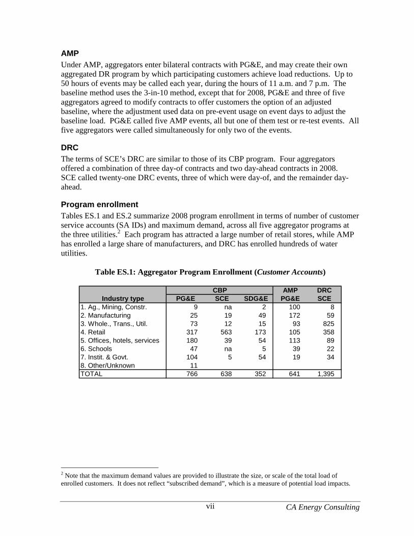
Program enrollment Tables ES.1 and ES.2 summarize 2008 program enrollment in terms of number of customer service accounts (SA IDs) and maximum demand, across all five aggregator programs at the three utilities.2 Each program has attracted a large number of retail stores, while AMP has enrolled a large share of manufacturers, and DRC has enrolled hundreds of water utilities.
Table ES.1: Aggregator Program Enrollment (Customer Accounts)
AMP DRC
Industry type PG&E SCE SDG&E PG&E SCE1. Ag., Mining, Constr. 9 na 2 100 82. Manufacturing 25 19 49 172 593. Whole., Trans., Util. 73 12 15 93 8254. Retail 317 563 173 105 3585. Offices, hotels, services 180 39 54 113 896. Schools 47 na 5 39 227. Instit. & Govt. 104 5 54 19 348. Other/Unknown 11TOTAL 766 638 352 641 1,395
CBP
2 Note that the maximum demand values are provided to illustrate the size, or scale of the total load of enrolled customers. It does not reflect “subscribed demand”, which is a measure of potential load impacts.
CA Energy Consulting viii
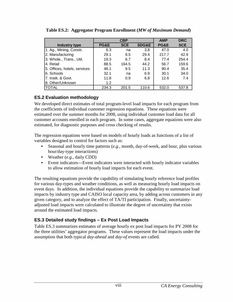
Table ES.2: Aggregator Program Enrollment (MW of Maximum Demand)
AMP DRCIndustry type PG&E SCE SDG&E PG&E SCE
1. Ag., Mining, Constr. 6.3 na 3.8 47.0 4.02. Manufacturing 29.1 9.5 29.4 217.7 42.93. Whole., Trans., Util. 19.3 6.7 8.4 77.4 254.44. Retail 88.5 164.5 44.2 56.7 159.65. Offices, hotels, services 46.1 9.5 11.3 90.4 35.46. Schools 32.1 na 6.9 30.1 34.07. Instit. & Govt. 11.8 0.9 6.8 12.6 7.48. Other/Unknown 1.2TOTAL 234.3 201.5 110.6 532.0 537.8
CBP
ES.2 Evaluation methodology We developed direct estimates of total program-level load impacts for each program from the coefficients of individual customer regression equations. These equations were estimated over the summer months for 2008, using individual customer load data for all customer accounts enrolled in each program. In some cases, aggregate equations were also estimated, for diagnostic purposes and cross checking of results. The regression equations were based on models of hourly loads as functions of a list of variables designed to control for factors such as:
• Seasonal and hourly time patterns (e.g., month, day-of-week, and hour, plus various hour/day-type interactions)
• Weather (e.g., daily CDD) • Event indicators—Event indicators were interacted with hourly indicator variables
to allow estimation of hourly load impacts for each event. The resulting equations provide the capability of simulating hourly reference load profiles for various day-types and weather conditions, as well as measuring hourly load impacts on event days. In addition, the individual equations provide the capability to summarize load impacts by industry type and CAISO local capacity area, by adding across customers in any given category, and to analyze the effect of TA/TI participation. Finally, uncertainty-adjusted load impacts were calculated to illustrate the degree of uncertainty that exists around the estimated load impacts.
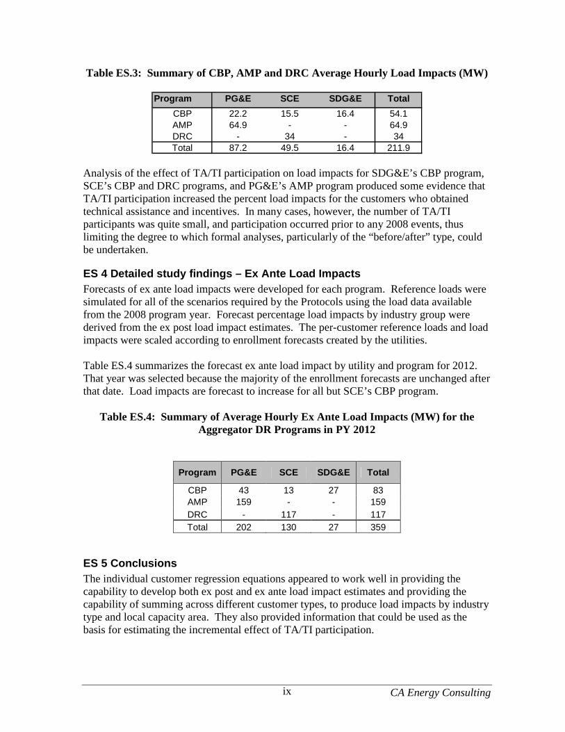
ES.3 Detailed study findings – Ex Post Load Impacts Table ES.3 summarizes estimates of average hourly ex post load impacts for PY 2008 for the three utilities’ aggregator programs. These values represent the load impacts under the assumption that both typical day-ahead and day-of events are called.
CA Energy Consulting ix
Table ES.3: Summary of CBP, AMP and DRC Average Hourly Load Impacts (MW)
Program PG&E SCE SDG&E Total
CBP 22.2 15.5 16.4 54.1AMP 64.9 - - 64.9DRC - 34 - 34Total 87.2 49.5 16.4 211.9
Analysis of the effect of TA/TI participation on load impacts for SDG&E’s CBP program, SCE’s CBP and DRC programs, and PG&E’s AMP program produced some evidence that TA/TI participation increased the percent load impacts for the customers who obtained technical assistance and incentives. In many cases, however, the number of TA/TI participants was quite small, and participation occurred prior to any 2008 events, thus limiting the degree to which formal analyses, particularly of the “before/after” type, could be undertaken.
ES 4 Detailed study findings – Ex Ante Load Impacts Forecasts of ex ante load impacts were developed for each program. Reference loads were simulated for all of the scenarios required by the Protocols using the load data available from the 2008 program year. Forecast percentage load impacts by industry group were derived from the ex post load impact estimates. The per-customer reference loads and load impacts were scaled according to enrollment forecasts created by the utilities. Table ES.4 summarizes the forecast ex ante load impact by utility and program for 2012. That year was selected because the majority of the enrollment forecasts are unchanged after that date. Load impacts are forecast to increase for all but SCE’s CBP program.
Table ES.4: Summary of Average Hourly Ex Ante Load Impacts (MW) for the
Aggregator DR Programs in PY 2012
Program PG&E SCE SDG&E Total
CBP 43 13 27 83 AMP 159 - - 159 DRC - 117 - 117 Total 202 130 27 359
ES 5 Conclusions The individual customer regression equations appeared to work well in providing the capability to develop both ex post and ex ante load impact estimates and providing the capability of summing across different customer types, to produce load impacts by industry type and local capacity area. They also provided information that could be used as the basis for estimating the incremental effect of TA/TI participation.
CA Energy Consulting 1
1. Introduction and Purpose of the Study This report documents the results of an evaluation of aggregator demand response (“DR”) programs operated by the three California investor-owned utilities (IOUs), Pacific Gas and Electric (“PG&E”), Southern California Edison (“SCE”), and San Diego Gas and Electric (“SDG&E”). An ex post analysis was performed for Program Year 2008 and an ex ante forecast was developed for 2009 through 2020. In these programs, aggregators contract with commercial and industrial customers to act on their behalf with respect to all aspects of the DR program, including receiving notices from the utility, arranging for load reductions on event days, receiving incentive payments, and paying penalties (if warranted) to the utility. Each aggregator forms a “portfolio” of individual customers such that their aggregated load participates in the DR programs. Aggregators receive both capacity credits for monthly nominated load reductions, regardless of whether events are called, and energy payments based on measured load reductions during events. The scope of this evaluation covers three price-responsive programs, including the state-wide Capacity Bidding Program (CPB), a tariff service operated by all three IOUs, Aggregator Managed Portfolio (AMP) operated by Pacific Gas and Electric (PG&E), and Demand Response Resource Contracts (DRC), operated by Southern California Edison (SCE). The latter two programs are implemented through bilateral contracts between utilities and the aggregators. The primary goals of this evaluation study were the following:
1. Assess the effectiveness of the aggregator programs; 2. Estimate the (ex post) load impacts for program year 2008; 3. Estimate ex ante load impacts for the programs for 2009 through 2020; and 4. Evaluate certain baseline issues.
The first goal involved a process evaluation consisting of interviews with program and aggregator staff, and surveys of participating customers, with the objective of assessing how effectively the programs have been administered and developing information on customer awareness and response to the programs. Results of the process evaluation are presented in Volume 3 of this report. The second goal involved estimating the hourly load impacts for each event, for each of the utilities’ aggregator programs. Our primary approach involved estimating individual customer regressions, which provided a flexible basis for analyzing and reporting load impact results at various levels (e.g., total program level) and by various factors (e.g., by industry group and CAISO local capacity area). The third goal involved combining the information on historical ex post load impacts with utility projections of program enrollment to produce forecasts of load impacts through 2020 for each of the programs. Key issues involved the detail by which the ex ante load impact forecasts must be presented, including the number of customer types and sizes. The last goal involved investigation of certain issues in measuring the baseline loads that are used to calculate aggregator load impacts for settlement purposes. Key issues included
CA Energy Consulting 2
assessing the relative accuracy of baselines developed at the aggregator level compared to those developed by summing individual customer-level baselines; assessing the effect of adjusting the baseline for differences in morning consumption on event days and on days used in constructing the baseline; assessing the degree to which gaming was avoided for those customers who selected the adjusted baseline approach; and assessing several alternatives to the current highest 3-in-10 baseline, including adjusted 5-in-10 and adjusted 10-in-10 baselines. The baseline analysis is documented in Volume 2 of this report. After this introductory section, Section 2 describes the aggregator programs, including the characteristics of the enrolled customer accounts. Section 3 discusses evaluation methodology. Section 4 presents ex-post load impacts. Section 5 describes the ex ante load. Section 6 discusses validity assessment, and Section 7 offers recommendations.
2. Description of Resources Covered in the Study This section summarizes the aggregator programs covered in this evaluation, including the characteristics of the participants in the programs.
2.1 Description of the aggregator programs
CBP The CBP program is a tariff service that provides monthly capacity payments ($/kW) based on amounts of load reductions that participating aggregators nominate each month, plus additional energy payments ($/kWh) based on the actual kWh reductions (relative to the program baseline) that are achieved when an event is called. Capacity penalties apply if events are called in a month and measured load reductions fall below 50 percent of nominated amounts. Participants may adjust their nomination each month, as well as their choice of available event type and window options (e.g., day-ahead (DA) or day-of (DO) events, and 4-hour or 6-hour event lengths). CBP events may be called on non-holiday weekdays in the months of May through October, between the hours of 11 a.m. and 7 p.m. Baseline loads, which serve as the basis for calculating load reductions for settlement, are calculated on the summed loads of an aggregated group of customers, based on the “highest 3-in-10” method. That is, the hourly baseline load during the event period is the hourly average across the three highest energy-usage (during program hours) days for the group out of the ten weekdays prior to the event (excluding holidays and previous event days). The “actual” load reduction in each hour is determined as the difference between the baseline load and the observed aggregated load in that hour. PG&E has six CBP aggregators, four of which offer day-ahead products and two of which offer both day-of and day-ahead products. SCE has six aggregator agreements, three of which offer day-of portfolios, two of which offer day-ahead portfolios, and one offers both. SDG&E has six CBP aggregators, four of which offer day-ahead products, one offers day-of products, and one offers both types.
CA Energy Consulting 3
AMP PG&E has five AMP bilateral aggregator contracts. Four aggregators offer day-of products, while one offers day-ahead products. Under AMP, aggregators may create their own aggregated DR program by which participating customers achieve load reductions. Up to 50 hours of events may be called each year, during the hours of 11 a.m. and 7 p.m. The baseline method is the 3-in-10 method, except that for 2008, PG&E and three of five aggregators agreed to modify contracts to offer customers the option of an adjusted baseline. The adjustment used the ratio of usage in the four hours prior to the event to usage in the same hours for the ten weekdays used in the 3-in-10 baseline, where the objective was to produce more accurate baselines for weather-sensitive customers.
DRC SCE has four DRC aggregators, which offered a combination of three day-of contracts and two day-ahead contracts in 2008. The terms of DRC are similar to those of SCE’s CBP program.
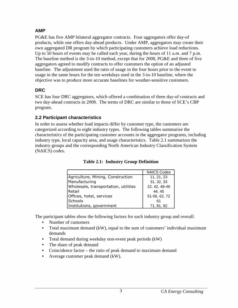
2.2 Participant characteristics In order to assess whether load impacts differ by customer type, the customers are categorized according to eight industry types. The following tables summarize the characteristics of the participating customer accounts in the aggregator programs, including industry type, local capacity area, and usage characteristics. Table 2.1 summarizes the industry groups and the corresponding North American Industry Classification System (NAICS) codes.
Table 2.1: Industry Group Definition
NAICS CodesAgriculture, Mining, Construction 11, 21, 23Manufacturing 31, 32, 33Wholesale, transportation, utilities 22, 42, 48-49Retail 44, 45Offices, hotel, services 51-56, 62, 72Schools 61Institutions, government 71, 81, 92
The participant tables show the following factors for each industry group and overall:
• Number of customers • Total maximum demand (kW), equal to the sum of customers’ individual maximum
demands • Total demand during weekday non-event peak periods (kW) • The share of peak demand • Coincidence factor – the ratio of peak demand to maximum demand • Average customer peak demand (kW).
CA Energy Consulting 4
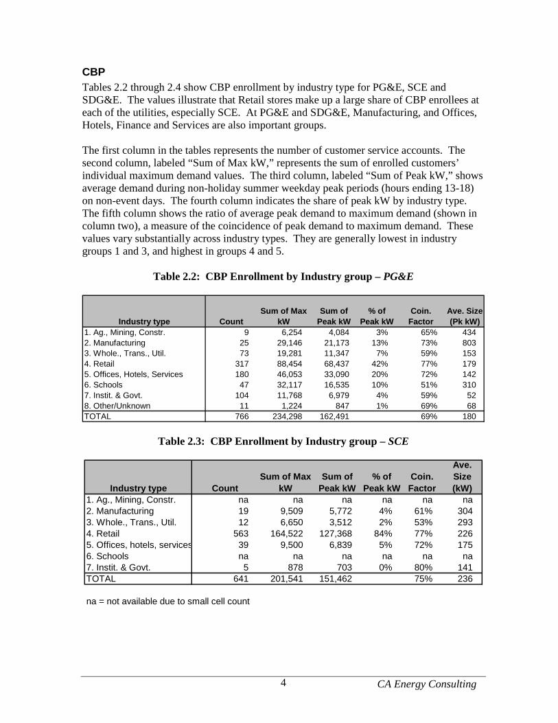
CBP Tables 2.2 through 2.4 show CBP enrollment by industry type for PG&E, SCE and SDG&E. The values illustrate that Retail stores make up a large share of CBP enrollees at each of the utilities, especially SCE. At PG&E and SDG&E, Manufacturing, and Offices, Hotels, Finance and Services are also important groups. The first column in the tables represents the number of customer service accounts. The second column, labeled “Sum of Max kW,” represents the sum of enrolled customers’ individual maximum demand values. The third column, labeled “Sum of Peak kW,” shows average demand during non-holiday summer weekday peak periods (hours ending 13-18) on non-event days. The fourth column indicates the share of peak kW by industry type. The fifth column shows the ratio of average peak demand to maximum demand (shown in column two), a measure of the coincidence of peak demand to maximum demand. These values vary substantially across industry types. They are generally lowest in industry groups 1 and 3, and highest in groups 4 and 5.
Table 2.2: CBP Enrollment by Industry group – PG&E
Industry type CountSum of Max
kWSum of
Peak kW% of
Peak kWCoin.
FactorAve. Size (Pk kW)
1. Ag., Mining, Constr. 9 6,254 4,084 3% 65% 4342. Manufacturing 25 29,146 21,173 13% 73% 8033. Whole., Trans., Util. 73 19,281 11,347 7% 59% 1534. Retail 317 88,454 68,437 42% 77% 1795. Offices, Hotels, Services 180 46,053 33,090 20% 72% 1426. Schools 47 32,117 16,535 10% 51% 3107. Instit. & Govt. 104 11,768 6,979 4% 59% 528. Other/Unknown 11 1,224 847 1% 69% 68TOTAL 766 234,298 162,491 69% 180
Table 2.3: CBP Enrollment by Industry group – SCE
Industry type CountSum of Max
kWSum of
Peak kW% of
Peak kWCoin. Factor
Ave. Size (kW)
1. Ag., Mining, Constr. na na na na na na2. Manufacturing 19 9,509 5,772 4% 61% 3043. Whole., Trans., Util. 12 6,650 3,512 2% 53% 2934. Retail 563 164,522 127,368 84% 77% 2265. Offices, hotels, services 39 9,500 6,839 5% 72% 1756. Schools na na na na na na7. Instit. & Govt. 5 878 703 0% 80% 141TOTAL 641 201,541 151,462 75% 236
na = not available due to small cell count
CA Energy Consulting 5
Table 2.4: CBP Enrollment by Industry group – SDG&E
Industry type CountSum of Max
kWSum of
Peak kW% of
Peak kWCoin.
Factor
Ave. Size (kW)
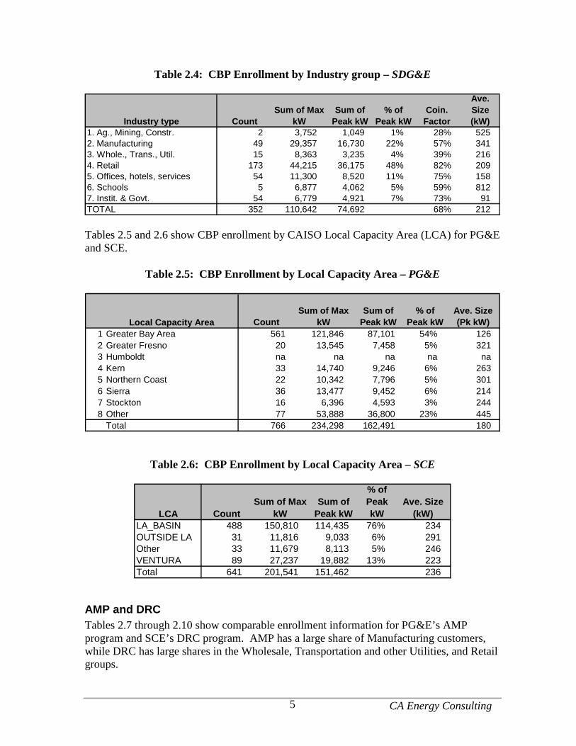
1. Ag., Mining, Constr. 2 3,752 1,049 1% 28% 5252. Manufacturing 49 29,357 16,730 22% 57% 3413. Whole., Trans., Util. 15 8,363 3,235 4% 39% 2164. Retail 173 44,215 36,175 48% 82% 2095. Offices, hotels, services 54 11,300 8,520 11% 75% 1586. Schools 5 6,877 4,062 5% 59% 8127. Instit. & Govt. 54 6,779 4,921 7% 73% 91TOTAL 352 110,642 74,692 68% 212 Tables 2.5 and 2.6 show CBP enrollment by CAISO Local Capacity Area (LCA) for PG&E and SCE.
Table 2.5: CBP Enrollment by Local Capacity Area – PG&E
Local Capacity Area CountSum of Max
kWSum of
Peak kW% of
Peak kWAve. Size (Pk kW)
1 Greater Bay Area 561 121,846 87,101 54% 1262 Greater Fresno 20 13,545 7,458 5% 3213 Humboldt na na na na na4 Kern 33 14,740 9,246 6% 2635 Northern Coast 22 10,342 7,796 5% 3016 Sierra 36 13,477 9,452 6% 2147 Stockton 16 6,396 4,593 3% 2448 Other 77 53,888 36,800 23% 445
Total 766 234,298 162,491 180
Table 2.6: CBP Enrollment by Local Capacity Area – SCE
LCA CountSum of Max
kWSum of
Peak kW
% of Peak kW
Ave. Size (kW)
LA_BASIN 488 150,810 114,435 76% 234OUTSIDE LA 31 11,816 9,033 6% 291Other 33 11,679 8,113 5% 246VENTURA 89 27,237 19,882 13% 223Total 641 201,541 151,462 236
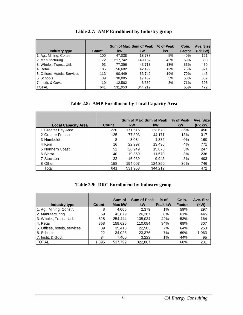
AMP and DRC Tables 2.7 through 2.10 show comparable enrollment information for PG&E’s AMP program and SCE’s DRC program. AMP has a large share of Manufacturing customers, while DRC has large shares in the Wholesale, Transportation and other Utilities, and Retail groups.
CA Energy Consulting 6
Table 2.7: AMP Enrollment by Industry group
Industry type CountSum of Max
kWSum of Peak
kW% of Peak
kWCoin. Factor
Ave. Size (Pk kW)
1. Ag., Mining, Constr. 100 47,038 18,738 5% 40% 1612. Manufacturing 172 217,742 149,167 43% 69% 8033. Whole., Trans., Util. 93 77,396 43,713 13% 56% 4504. Retail 105 56,682 42,499 12% 75% 3215. Offices, Hotels, Services 113 90,449 63,749 19% 70% 4436. Schools 39 30,085 17,487 5% 58% 3877. Instit. & Govt. 19 12,562 8,859 3% 71% 396TOTAL 641 531,953 344,212 65% 472
Table 2.8: AMP Enrollment by Local Capacity Area
Local Capacity Area CountSum of Max
kWSum of Peak
kW% of Peak
kWAve. Size (Pk kW)
1 Greater Bay Area 220 171,515 123,678 36% 4562 Greater Fresno 125 77,803 44,171 13% 3173 Humboldt 8 3,034 1,332 0% 1604 Kern 16 22,297 13,496 4% 7715 Northern Coast 52 26,949 15,673 5% 2476 Sierra 40 19,359 11,570 3% 2367 Stockton 22 16,989 9,943 3% 4038 Other 158 194,007 124,350 36% 746
Total 641 531,953 344,212 472
Table 2.9: DRC Enrollment by Industry group
Industry type CountSum of Max kW
Sum of Peak kW
% of Peak kW
Coin. Factor
Ave. Size (kW)
1. Ag., Mining, Constr. 8 4,005 2,379 1% 59% 2972. Manufacturing 59 42,879 26,267 8% 61% 4453. Whole., Trans., Util. 825 254,444 135,034 42% 53% 1644. Retail 358 159,626 110,084 34% 69% 3075. Offices, hotels, services 89 35,413 22,503 7% 64% 2536. Schools 22 34,026 23,376 7% 69% 1,0637. Instit. & Govt. 34 7,400 3,223 1% 44% 95TOTAL 1,395 537,792 322,867 60% 231
CA Energy Consulting 7
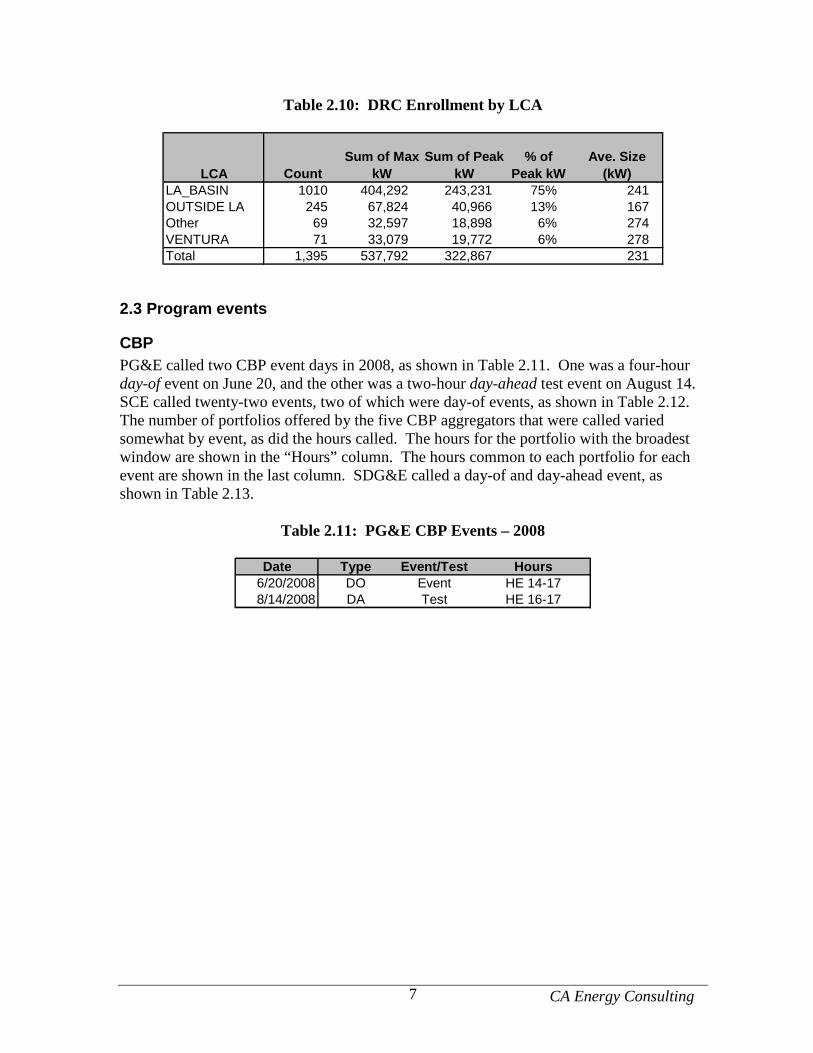
Table 2.10: DRC Enrollment by LCA
LCA CountSum of Max
kWSum of Peak
kW% of
Peak kWAve. Size
(kW)LA_BASIN 1010 404,292 243,231 75% 241OUTSIDE LA 245 67,824 40,966 13% 167Other 69 32,597 18,898 6% 274VENTURA 71 33,079 19,772 6% 278Total 1,395 537,792 322,867 231
2.3 Program events
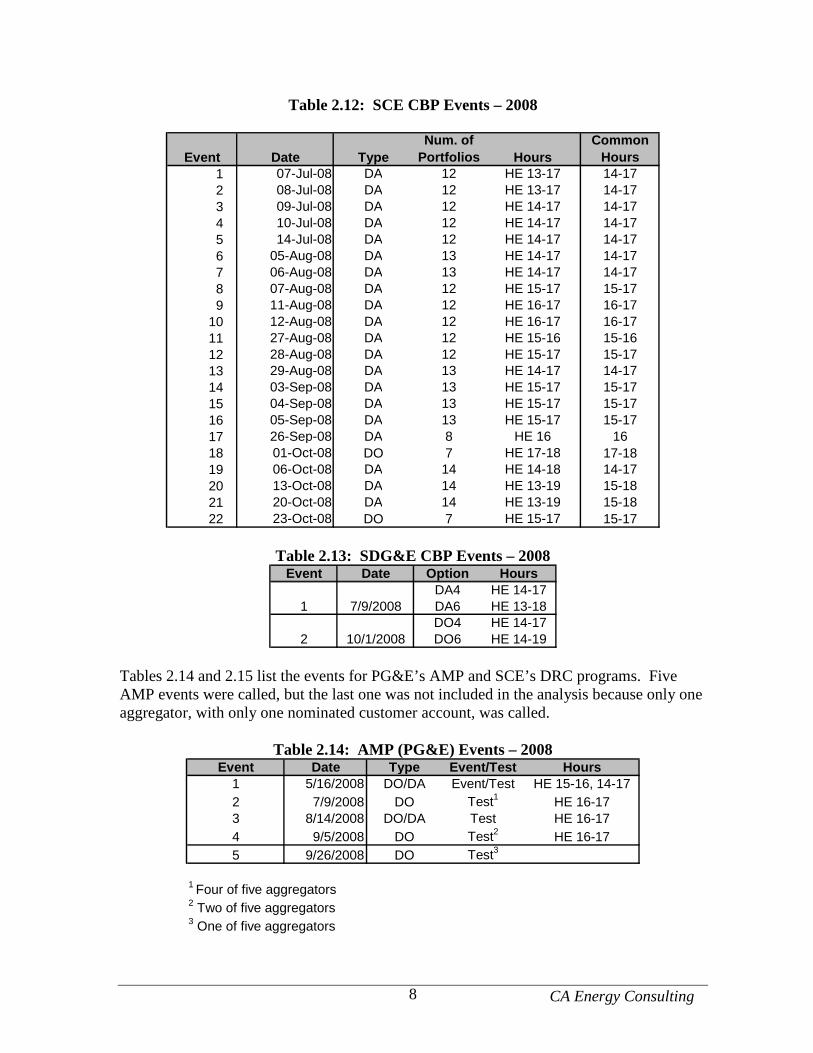
CBP PG&E called two CBP event days in 2008, as shown in Table 2.11. One was a four-hour day-of event on June 20, and the other was a two-hour day-ahead test event on August 14. SCE called twenty-two events, two of which were day-of events, as shown in Table 2.12. The number of portfolios offered by the five CBP aggregators that were called varied somewhat by event, as did the hours called. The hours for the portfolio with the broadest window are shown in the “Hours” column. The hours common to each portfolio for each event are shown in the last column. SDG&E called a day-of and day-ahead event, as shown in Table 2.13.
Table 2.11: PG&E CBP Events – 2008
Date Type Event/Test Hours6/20/2008 DO Event HE 14-178/14/2008 DA Test HE 16-17
CA Energy Consulting 8
Table 2.12: SCE CBP Events – 2008
Event Date TypeNum. of
Portfolios HoursCommon
Hours1 07-Jul-08 DA 12 HE 13-17 14-172 08-Jul-08 DA 12 HE 13-17 14-173 09-Jul-08 DA 12 HE 14-17 14-174 10-Jul-08 DA 12 HE 14-17 14-175 14-Jul-08 DA 12 HE 14-17 14-176 05-Aug-08 DA 13 HE 14-17 14-177 06-Aug-08 DA 13 HE 14-17 14-178 07-Aug-08 DA 12 HE 15-17 15-179 11-Aug-08 DA 12 HE 16-17 16-17
10 12-Aug-08 DA 12 HE 16-17 16-1711 27-Aug-08 DA 12 HE 15-16 15-1612 28-Aug-08 DA 12 HE 15-17 15-1713 29-Aug-08 DA 13 HE 14-17 14-1714 03-Sep-08 DA 13 HE 15-17 15-1715 04-Sep-08 DA 13 HE 15-17 15-1716 05-Sep-08 DA 13 HE 15-17 15-1717 26-Sep-08 DA 8 HE 16 1618 01-Oct-08 DO 7 HE 17-18 17-1819 06-Oct-08 DA 14 HE 14-18 14-1720 13-Oct-08 DA 14 HE 13-19 15-1821 20-Oct-08 DA 14 HE 13-19 15-1822 23-Oct-08 DO 7 HE 15-17 15-17
Table 2.13: SDG&E CBP Events – 2008
Event Date Option HoursDA4 HE 14-17DA6 HE 13-18DO4 HE 14-17DO6 HE 14-19
1
2
7/9/2008
10/1/2008
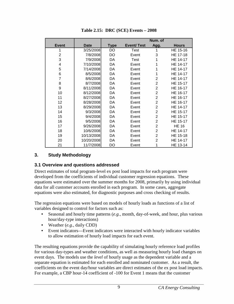
Tables 2.14 and 2.15 list the events for PG&E’s AMP and SCE’s DRC programs. Five AMP events were called, but the last one was not included in the analysis because only one aggregator, with only one nominated customer account, was called.
Table 2.14: AMP (PG&E) Events – 2008 Event Date Type Event/Test Hours
1 5/16/2008 DO/DA Event/Test HE 15-16, 14-172 7/9/2008 DO Test1 HE 16-173 8/14/2008 DO/DA Test HE 16-174 9/5/2008 DO Test2 HE 16-175 9/26/2008 DO Test3
1 Four of five aggregators2 Two of five aggregators3 One of five aggregators
CA Energy Consulting 9
Table 2.15: DRC (SCE) Events – 2008
Event Date Type Event/ TestNum. of
Agg. Hours1 3/25/2008 DO Test 1 HE 15-162 7/8/2008 DO Event 3 HE 17-183 7/9/2008 DA Test 1 HE 14-174 7/10/2008 DA Event 1 HE 14-175 7/14/2008 DA Event 1 HE 14-176 8/5/2008 DA Event 1 HE 14-177 8/6/2008 DA Event 2 HE 14-178 8/7/2008 DA Event 2 HE 15-179 8/11/2008 DA Event 2 HE 16-1710 8/12/2008 DA Event 2 HE 16-1711 8/27/2008 DA Event 2 HE 16-1712 8/28/2008 DA Event 2 HE 16-1713 8/29/2008 DA Event 2 HE 14-1714 9/3/2008 DA Event 2 HE 15-1715 9/4/2008 DA Event 2 HE 15-1716 9/5/2008 DA Event 2 HE 15-1717 9/26/2008 DA Event 2 HE 1618 10/6/2008 DA Event 2 HE 14-1719 10/13/2008 DA Event 2 HE 15-1820 10/20/2008 DA Event 2 HE 14-1721 11/7/2008 DO Event 1 HE 13-14
3. Study Methodology
3.1 Overview and questions addressed Direct estimates of total program-level ex post load impacts for each program were developed from the coefficients of individual customer regression equations. These equations were estimated over the summer months for 2008, primarily by using individual data for all customer accounts enrolled in each program. In some cases, aggregate equations were also estimated, for diagnostic purposes and cross checking of results. The regression equations were based on models of hourly loads as functions of a list of variables designed to control for factors such as:
• Seasonal and hourly time patterns (e.g., month, day-of-week, and hour, plus various hour/day-type interactions)
• Weather (e.g., daily CDD) • Event indicators—Event indicators were interacted with hourly indicator variables
to allow estimation of hourly load impacts for each event. The resulting equations provide the capability of simulating hourly reference load profiles for various day-types and weather conditions, as well as measuring hourly load changes on event days. The models use the level of hourly usage as the dependent variable and a separate equation is estimated for each enrolled and nominated customer. As a result, the coefficients on the event day/hour variables are direct estimates of the ex post load impacts. For example, a CBP hour-14 coefficient of -100 for Event 1 means that the customer
CA Energy Consulting 10
reduced load by 100 kWh during hour 14 of that event day relative to its normal usage in that hour. Weekends and holidays were excluded from the estimation database.3 Finally, uncertainty-adjusted load impacts were calculated to illustrate the degree of statistical confidence that exists around the estimated load impacts.
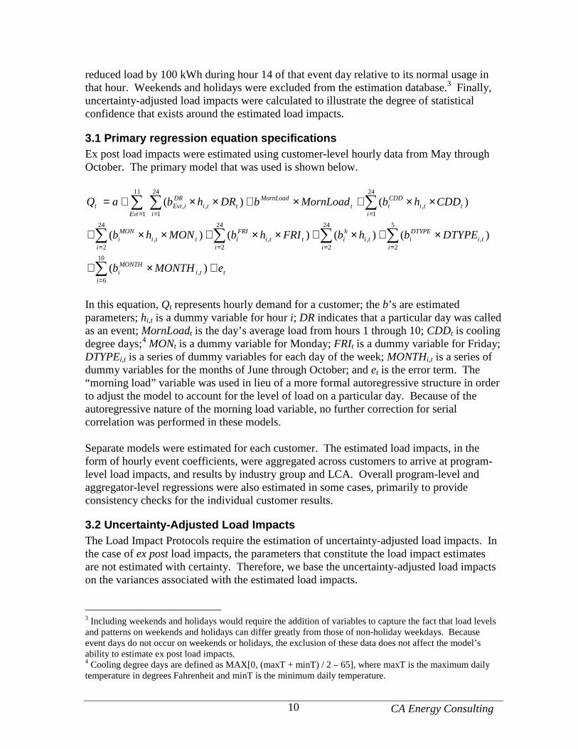
3.1 Primary regression equation specifications Ex post load impacts were estimated using customer-level hourly data from May through October. The primary model that was used is shown below.
ti
tiMONTHi
iti
DTYPEi
iti
hi
itti
FRIi
itti
MONi
i itti
CDDit
MornLoadtti
DRiEvt
Evtt
eMONTHb
DTYPEbhbFRIhbMONhb
CDDhbMornLoadbDRhbaQ
+×+
×+×+××+××+
××+×+××+=
∑
∑∑∑∑
∑ ∑∑
=
====
= ==
)(
)()()()(
)()(
10
6,
5
2,
24
2,
24
2,
24
2,
24
1
24
1,,,
11
1
In this equation, Qt represents hourly demand for a customer; the b’s are estimated parameters; hi,t is a dummy variable for hour i; DR indicates that a particular day was called as an event; MornLoadt is the day’s average load from hours 1 through 10; CDDt is cooling degree days;4 MONt is a dummy variable for Monday; FRIt is a dummy variable for Friday; DTYPEi,t is a series of dummy variables for each day of the week; MONTHi,t is a series of dummy variables for the months of June through October; and et is the error term. The “morning load” variable was used in lieu of a more formal autoregressive structure in order to adjust the model to account for the level of load on a particular day. Because of the autoregressive nature of the morning load variable, no further correction for serial correlation was performed in these models. Separate models were estimated for each customer. The estimated load impacts, in the form of hourly event coefficients, were aggregated across customers to arrive at program-level load impacts, and results by industry group and LCA. Overall program-level and aggregator-level regressions were also estimated in some cases, primarily to provide consistency checks for the individual customer results.
3.2 Uncertainty-Adjusted Load Impacts The Load Impact Protocols require the estimation of uncertainty-adjusted load impacts. In the case of ex post load impacts, the parameters that constitute the load impact estimates are not estimated with certainty. Therefore, we base the uncertainty-adjusted load impacts on the variances associated with the estimated load impacts.
3 Including weekends and holidays would require the addition of variables to capture the fact that load levels and patterns on weekends and holidays can differ greatly from those of non-holiday weekdays. Because event days do not occur on weekends or holidays, the exclusion of these data does not affect the model’s ability to estimate ex post load impacts. 4 Cooling degree days are defined as MAX[0, (maxT + minT) / 2 – 65], where maxT is the maximum daily temperature in degrees Fahrenheit and minT is the minimum daily temperature.
CA Energy Consulting 11
Specifically, we add the variances of the estimated load impacts across the customers who were nominated for the event in question. These aggregations are performed at either the program level, by industry group, or by LCA. The uncertainty-adjusted scenarios were then simulated under the assumption that each hour’s load impact is normally distributed with the mean equal to the sum of the estimated load impacts and the standard deviation equal to the square root of the sum of the variances of the errors around the estimates of the load impacts. Results for the 10th, 30th, 70th, and 90th percentile scenarios are generated from these distributions.
4. Detailed Study Findings This section describes the results of our estimation of aggregate and per-customer event-day load impacts for each aggregator program and each utility. For each program, we begin by summarizing the load impacts estimated for 2008, using estimates of average hourly load impacts for each event, and, where relevant, for average or typical events. We then provide the formal tables required by the Protocols, including reference loads, observed loads, and load impacts by hour, and uncertainty-adjusted load impacts at different probability levels. Load impact results are also illustrated in figures. We also provide illustrative graphs of the observed aggregated program load on selected event-days and non-event days as a form of real-world confirmation of the estimated load impacts. We begin with CBP at each of the three utilities, and then turn to AMP and DRC.
4.1 CBP
4.1.1 PG&E5 Program-level load impacts
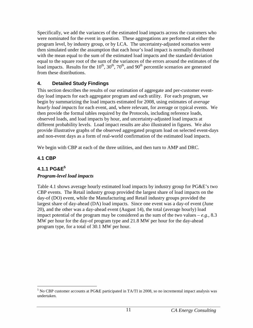
Table 4.1 shows average hourly estimated load impacts by industry group for PG&E’s two CBP events. The Retail industry group provided the largest share of load impacts on the day-of (DO) event, while the Manufacturing and Retail industry groups provided the largest share of day-ahead (DA) load impacts. Since one event was a day-of event (June 20), and the other was a day-ahead event (August 14), the total (average hourly) load impact potential of the program may be considered as the sum of the two values – e.g., 8.3 MW per hour for the day-of program type and 21.8 MW per hour for the day-ahead program type, for a total of 30.1 MW per hour.
5 No CBP customer accounts at PG&E participated in TA/TI in 2008, so no incremental impact analysis was undertaken.
CA Energy Consulting 12
Table 4.1: PG&E CBP Average Hourly Load Impacts, by Industry Group (kW)
Evt 1 (DO) Evt 2 (DA)Industry type 20-Jun 14-Aug1. Ag., Mining, Constr. 0 942. Manufacturing -11 5,8223. Whole., Trans., Util. 1,716 1,2434. Retail 4,117 5,9505. Offices, Hotels, Services 172 5106. Schools 216 2,0377. Instit. & Govt. 0 3208. Other/Unknown 0 44TOTAL 6,211 16,020
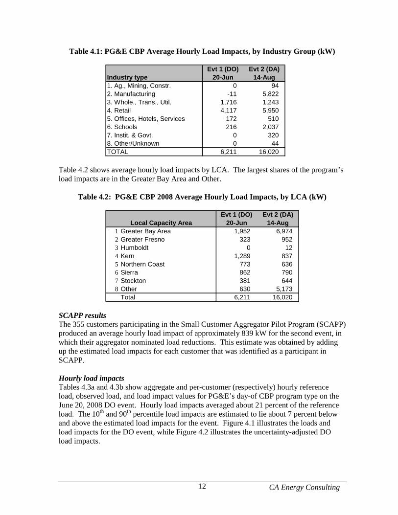
Table 4.2 shows average hourly load impacts by LCA. The largest shares of the program’s load impacts are in the Greater Bay Area and Other.
Table 4.2: PG&E CBP 2008 Average Hourly Load Impacts, by LCA (kW)
Evt 1 (DO) Evt 2 (DA)20-Jun 14-Aug
1 Greater Bay Area 1,952 6,9742 Greater Fresno 323 9523 Humboldt 0 124 Kern 1,289 8375 Northern Coast 773 6366 Sierra 862 7907 Stockton 381 6448 Other 630 5,173
Total 6,211 16,020
Local Capacity Area
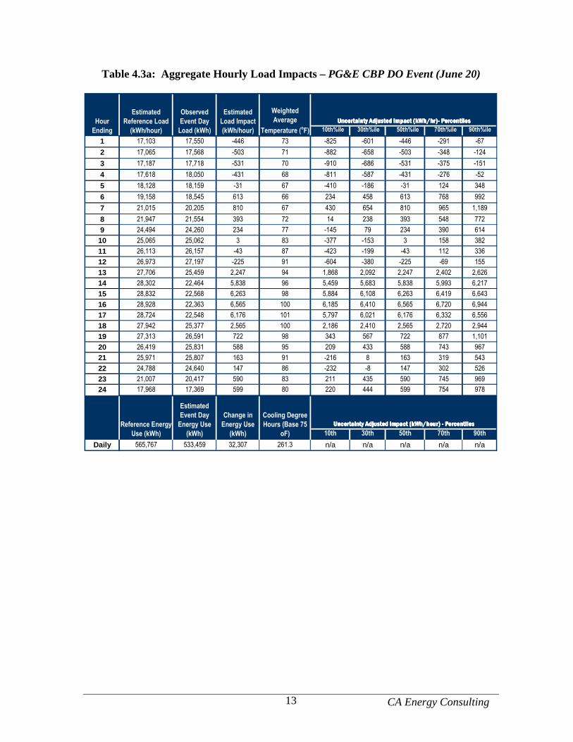
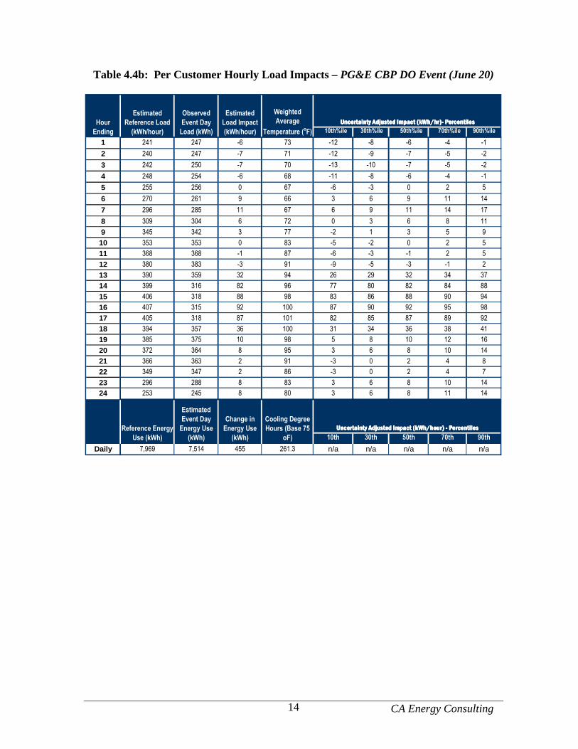
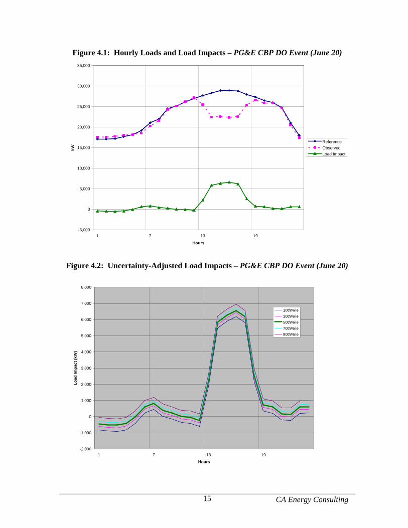
SCAPP results The 355 customers participating in the Small Customer Aggregator Pilot Program (SCAPP) produced an average hourly load impact of approximately 839 kW for the second event, in which their aggregator nominated load reductions. This estimate was obtained by adding up the estimated load impacts for each customer that was identified as a participant in SCAPP. Hourly load impacts Tables 4.3a and 4.3b show aggregate and per-customer (respectively) hourly reference load, observed load, and load impact values for PG&E’s day-of CBP program type on the June 20, 2008 DO event. Hourly load impacts averaged about 21 percent of the reference load. The 10th and 90th percentile load impacts are estimated to lie about 7 percent below and above the estimated load impacts for the event. Figure 4.1 illustrates the loads and load impacts for the DO event, while Figure 4.2 illustrates the uncertainty-adjusted DO load impacts.
CA Energy Consulting 13
Table 4.3a: Aggregate Hourly Load Impacts – PG&E CBP DO Event (June 20)
Uncertainty Adjusted Impact (kWh/hr)- PercentilesUncertainty Adjusted Impact (kWh/hr)- PercentilesUncertainty Adjusted Impact (kWh/hr)- PercentilesUncertainty Adjusted Impact (kWh/hr)- Percentiles
10th%ile 30th%ile 50th%ile 70th%ile 90th%ile
1 17,103 17,550 -446 73 -825 -601 -446 -291 -67
2 17,065 17,568 -503 71 -882 -658 -503 -348 -124
3 17,187 17,718 -531 70 -910 -686 -531 -375 -151
4 17,618 18,050 -431 68 -811 -587 -431 -276 -52
5 18,128 18,159 -31 67 -410 -186 -31 124 348
6 19,158 18,545 613 66 234 458 613 768 992
7 21,015 20,205 810 67 430 654 810 965 1,189
8 21,947 21,554 393 72 14 238 393 548 772
9 24,494 24,260 234 77 -145 79 234 390 614
10 25,065 25,062 3 83 -377 -153 3 158 382
11 26,113 26,157 -43 87 -423 -199 -43 112 336
12 26,973 27,197 -225 91 -604 -380 -225 -69 155
13 27,706 25,459 2,247 94 1,868 2,092 2,247 2,402 2,626
14 28,302 22,464 5,838 96 5,459 5,683 5,838 5,993 6,217
15 28,832 22,568 6,263 98 5,884 6,108 6,263 6,419 6,643
16 28,928 22,363 6,565 100 6,185 6,410 6,565 6,720 6,944
17 28,724 22,548 6,176 101 5,797 6,021 6,176 6,332 6,556
18 27,942 25,377 2,565 100 2,186 2,410 2,565 2,720 2,944
19 27,313 26,591 722 98 343 567 722 877 1,101
20 26,419 25,831 588 95 209 433 588 743 967
21 25,971 25,807 163 91 -216 8 163 319 543
22 24,788 24,640 147 86 -232 -8 147 302 526
23 21,007 20,417 590 83 211 435 590 745 969
24 17,968 17,369 599 80 220 444 599 754 978
Uncertainty Adjusted Impact (kWh/hour) - PercentilesUncertainty Adjusted Impact (kWh/hour) - PercentilesUncertainty Adjusted Impact (kWh/hour) - PercentilesUncertainty Adjusted Impact (kWh/hour) - Percentiles
10th 30th 50th 70th 90th
Daily 565,767 533,459 32,307 261.3 n/a n/a n/a n/a n/a
Weighted
Average
Temperature (oF)
Reference Energy
Use (kWh)
Estimated
Event Day
Energy Use
(kWh)
Change in
Energy Use
(kWh)
Cooling Degree
Hours (Base 75
oF)
Hour
Ending
Estimated
Reference Load
(kWh/hour)
Observed
Event Day
Load (kWh)
Estimated
Load Impact
(kWh/hour)
CA Energy Consulting 14
Table 4.4b: Per Customer Hourly Load Impacts – PG&E CBP DO Event (June 20)
Uncertainty Adjusted Impact (kWh/hr)- PercentilesUncertainty Adjusted Impact (kWh/hr)- PercentilesUncertainty Adjusted Impact (kWh/hr)- PercentilesUncertainty Adjusted Impact (kWh/hr)- Percentiles
10th%ile 30th%ile 50th%ile 70th%ile 90th%ile
1 241 247 -6 73 -12 -8 -6 -4 -1
2 240 247 -7 71 -12 -9 -7 -5 -2
3 242 250 -7 70 -13 -10 -7 -5 -2
4 248 254 -6 68 -11 -8 -6 -4 -1
5 255 256 0 67 -6 -3 0 2 5
6 270 261 9 66 3 6 9 11 14
7 296 285 11 67 6 9 11 14 17
8 309 304 6 72 0 3 6 8 11
9 345 342 3 77 -2 1 3 5 9
10 353 353 0 83 -5 -2 0 2 5
11 368 368 -1 87 -6 -3 -1 2 5
12 380 383 -3 91 -9 -5 -3 -1 2
13 390 359 32 94 26 29 32 34 37
14 399 316 82 96 77 80 82 84 88
15 406 318 88 98 83 86 88 90 94
16 407 315 92 100 87 90 92 95 98
17 405 318 87 101 82 85 87 89 92
18 394 357 36 100 31 34 36 38 41
19 385 375 10 98 5 8 10 12 16
20 372 364 8 95 3 6 8 10 14
21 366 363 2 91 -3 0 2 4 8
22 349 347 2 86 -3 0 2 4 7
23 296 288 8 83 3 6 8 10 14
24 253 245 8 80 3 6 8 11 14
Uncertainty Adjusted Impact (kWh/hour) - PercentilesUncertainty Adjusted Impact (kWh/hour) - PercentilesUncertainty Adjusted Impact (kWh/hour) - PercentilesUncertainty Adjusted Impact (kWh/hour) - Percentiles
10th 30th 50th 70th 90th
Daily 7,969 7,514 455 261.3 n/a n/a n/a n/a n/a
Hour
Ending
Estimated
Reference Load
(kWh/hour)
Observed
Event Day
Load (kWh)
Estimated
Load Impact
(kWh/hour)
Weighted
Average
Temperature (oF)
Reference Energy
Use (kWh)
Estimated
Event Day
Energy Use
(kWh)
Change in
Energy Use
(kWh)
Cooling Degree
Hours (Base 75
oF)
CA Energy Consulting 15
Figure 4.1: Hourly Loads and Load Impacts – PG&E CBP DO Event (June 20)
-5,000
0
5,000
10,000
15,000
20,000
25,000
30,000
35,000
1 7 13 19
Hours
kW
Reference
Observed
Load Impact
Figure 4.2: Uncertainty-Adjusted Load Impacts – PG&E CBP DO Event (June 20)
-2,000
-1,000
0
1,000
2,000
3,000
4,000
5,000
6,000
7,000
8,000
1 7 13 19
Hours
Load
Impa
ct (
kW)
10th%ile
30th%ile
50th%ile
70th%ile
90th%ile
CA Energy Consulting 16
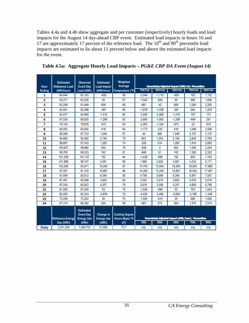
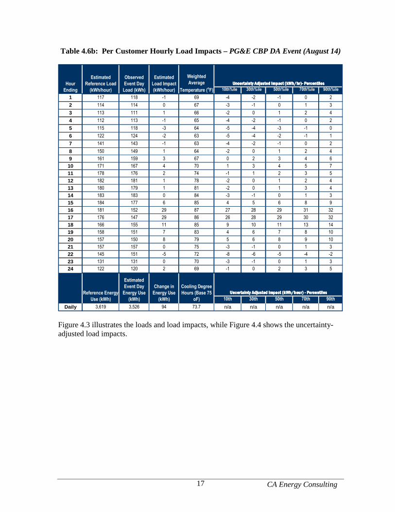
Tables 4.4a and 4.4b show aggregate and per customer (respectively) hourly loads and load impacts for the August 14 day-ahead CBP event. Estimated load impacts in hours 16 and 17 are approximately 17 percent of the reference load. The 10th and 90th percentile load impacts are estimated to lie about 11 percent below and above the estimated load impacts for the event.
Table 4.5a: Aggregate Hourly Load Impacts – PG&E CBP DA Event (August 14)
Uncertainty Adjusted Impact (kWh/hr)- PercentilesUncertainty Adjusted Impact (kWh/hr)- PercentilesUncertainty Adjusted Impact (kWh/hr)- PercentilesUncertainty Adjusted Impact (kWh/hr)- Percentiles
10th%ile 30th%ile 50th%ile 70th%ile 90th%ile
1 64,644 65,103 -459 69 -2,049 -1,110 -459 192 1,132
2 63,271 63,226 45 67 -1,545 -606 45 696 1,636
3 62,258 61,648 609 66 -981 -42 609 1,260 2,200
4 62,001 62,388 -387 65 -1,978 -1,038 -387 264 1,203
5 63,577 64,995 -1,418 64 -3,008 -2,069 -1,418 -767 173
6 67,530 68,830 -1,299 63 -2,890 -1,950 -1,299 -649 291
7 78,152 78,825 -673 63 -2,263 -1,324 -673 -22 918
8 83,052 82,634 418 64 -1,173 -233 418 1,069 2,008
9 89,269 87,723 1,546 67 -44 895 1,546 2,197 3,137
10 94,685 92,492 2,194 70 603 1,543 2,194 2,845 3,784
11 98,697 97,433 1,265 74 -326 614 1,265 1,916 2,855
12 100,637 99,984 653 78 -938 2 653 1,304 2,244
13 99,765 99,023 742 81 -848 91 742 1,393 2,333
14 101,258 101,107 152 84 -1,439 -499 152 803 1,742
15 101,688 98,107 3,581 85 1,990 2,930 3,581 4,232 5,171
16 100,265 83,971 16,294 87 14,704 15,644 16,294 16,945 17,885
17 97,207 81,316 15,891 86 14,300 15,240 15,891 16,542 17,481
18 91,959 85,612 6,346 85 4,756 5,696 6,346 6,997 7,937
19 87,491 83,566 3,925 83 2,334 3,274 3,925 4,576 5,516
20 87,030 82,823 4,207 79 2,616 3,556 4,207 4,858 5,798
21 87,093 87,040 53 75 -1,538 -598 53 703 1,643
22 80,405 83,243 -2,839 72 -4,429 -3,490 -2,839 -2,188 -1,248
23 72,258 72,222 35 70 -1,555 -616 35 686 1,626
24 67,315 66,392 924 69 -667 273 924 1,575 2,514
Uncertainty Adjusted Impact (kWh/hour) - PercentilesUncertainty Adjusted Impact (kWh/hour) - PercentilesUncertainty Adjusted Impact (kWh/hour) - PercentilesUncertainty Adjusted Impact (kWh/hour) - Percentiles
10th 30th 50th 70th 90th
Daily 2,001,509 1,949,703 51,806 73.7 n/a n/a n/a n/a n/a
Weighted
Average
Temperature (oF)
Reference Energy
Use (kWh)
Estimated
Event Day
Energy Use
(kWh)
Change in
Energy Use
(kWh)
Cooling Degree
Hours (Base 75
oF)
Hour
Ending
Estimated
Reference Load
(kWh/hour)
Observed
Event Day
Load (kWh)
Estimated
Load Impact
(kWh/hour)
CA Energy Consulting 17
Table 4.6b: Per Customer Hourly Load Impacts – PG&E CBP DA Event (August 14)
Uncertainty Adjusted Impact (kWh/hr)- PercentilesUncertainty Adjusted Impact (kWh/hr)- PercentilesUncertainty Adjusted Impact (kWh/hr)- PercentilesUncertainty Adjusted Impact (kWh/hr)- Percentiles
10th%ile 30th%ile 50th%ile 70th%ile 90th%ile
1 117 118 -1 69 -4 -2 -1 0 2
2 114 114 0 67 -3 -1 0 1 3
3 113 111 1 66 -2 0 1 2 4
4 112 113 -1 65 -4 -2 -1 0 2
5 115 118 -3 64 -5 -4 -3 -1 0
6 122 124 -2 63 -5 -4 -2 -1 1
7 141 143 -1 63 -4 -2 -1 0 2
8 150 149 1 64 -2 0 1 2 4
9 161 159 3 67 0 2 3 4 6
10 171 167 4 70 1 3 4 5 7
11 178 176 2 74 -1 1 2 3 5
12 182 181 1 78 -2 0 1 2 4
13 180 179 1 81 -2 0 1 3 4
14 183 183 0 84 -3 -1 0 1 3
15 184 177 6 85 4 5 6 8 9
16 181 152 29 87 27 28 29 31 32
17 176 147 29 86 26 28 29 30 32
18 166 155 11 85 9 10 11 13 14
19 158 151 7 83 4 6 7 8 10
20 157 150 8 79 5 6 8 9 10
21 157 157 0 75 -3 -1 0 1 3
22 145 151 -5 72 -8 -6 -5 -4 -2
23 131 131 0 70 -3 -1 0 1 3
24 122 120 2 69 -1 0 2 3 5
Uncertainty Adjusted Impact (kWh/hour) - PercentilesUncertainty Adjusted Impact (kWh/hour) - PercentilesUncertainty Adjusted Impact (kWh/hour) - PercentilesUncertainty Adjusted Impact (kWh/hour) - Percentiles
10th 30th 50th 70th 90th
Daily 3,619 3,526 94 73.7 n/a n/a n/a n/a n/a
Hour
Ending
Estimated
Reference Load
(kWh/hour)
Observed
Event Day
Load (kWh)
Estimated
Load Impact
(kWh/hour)
Weighted
Average
Temperature (oF)
Reference Energy
Use (kWh)
Estimated
Event Day
Energy Use
(kWh)
Change in
Energy Use
(kWh)
Cooling Degree
Hours (Base 75
oF)
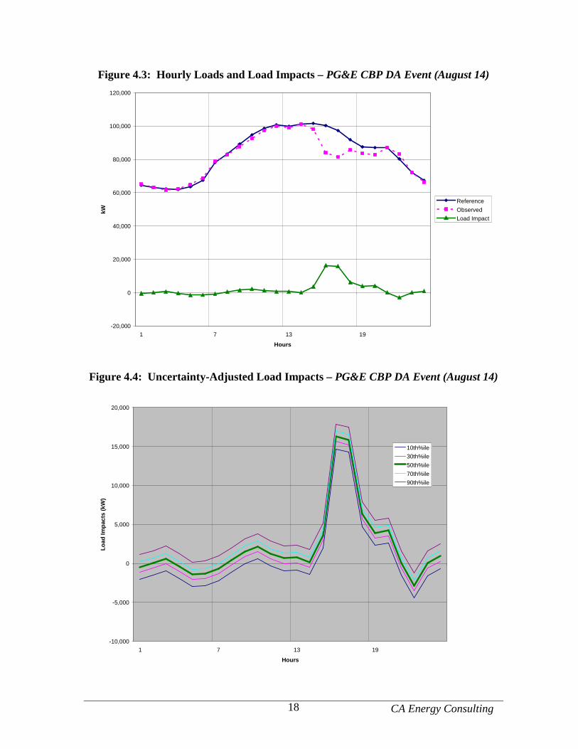
Figure 4.3 illustrates the loads and load impacts, while Figure 4.4 shows the uncertainty-adjusted load impacts.
CA Energy Consulting 18
Figure 4.3: Hourly Loads and Load Impacts – PG&E CBP DA Event (August 14)
-20,000
0
20,000
40,000
60,000
80,000
100,000
120,000
1 7 13 19
Hours
kW
Reference
Observed
Load Impact
Figure 4.4: Uncertainty-Adjusted Load Impacts – PG&E CBP DA Event (August 14)
-10,000
-5,000
0
5,000
10,000
15,000
20,000
1 7 13 19
Hours
Load
Impa
cts
(kW
)
10th%ile
30th%ile
50th%ile
70th%ile
90th%ile
CA Energy Consulting 19
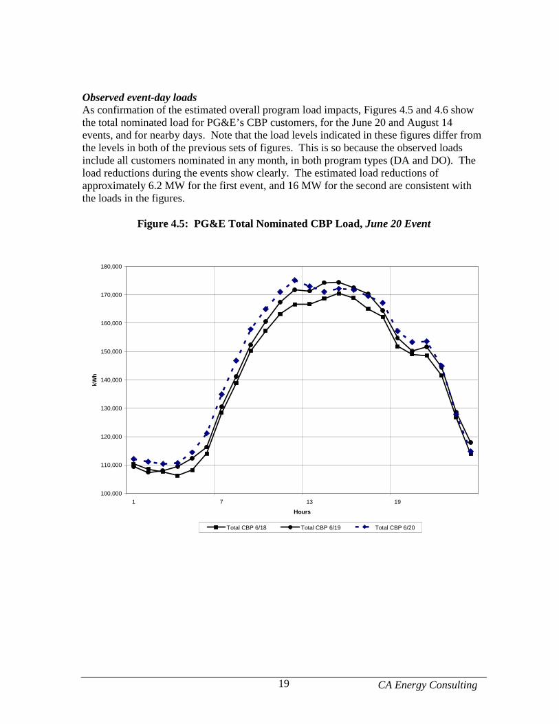
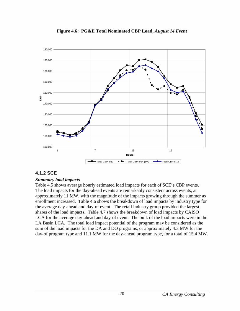
Observed event-day loads As confirmation of the estimated overall program load impacts, Figures 4.5 and 4.6 show the total nominated load for PG&E’s CBP customers, for the June 20 and August 14 events, and for nearby days. Note that the load levels indicated in these figures differ from the levels in both of the previous sets of figures. This is so because the observed loads include all customers nominated in any month, in both program types (DA and DO). The load reductions during the events show clearly. The estimated load reductions of approximately 6.2 MW for the first event, and 16 MW for the second are consistent with the loads in the figures.
Figure 4.5: PG&E Total Nominated CBP Load, June 20 Event
100,000
110,000
120,000
130,000
140,000
150,000
160,000
170,000
180,000
1 7 13 19
Hours
kWh
Total CBP 6/18 Total CBP 6/19 Total CBP 6/20
CA Energy Consulting 20
Figure 4.6: PG&E Total Nominated CBP Load, August 14 Event
100,000
110,000
120,000
130,000
140,000
150,000
160,000
170,000
180,000
190,000
1 7 13 19
Hours
kWh
Total CBP 8/13 Total CBP 8/14 (evt) Total CBP 8/15
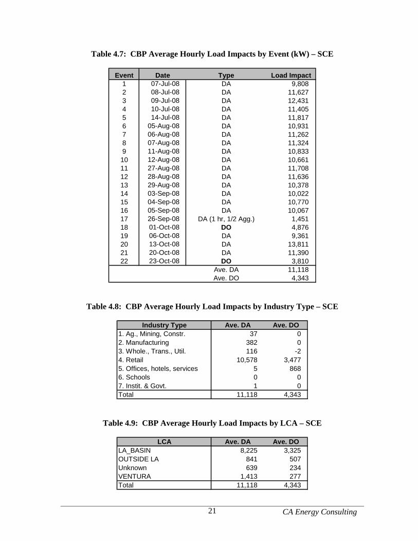
4.1.2 SCE Summary load impacts Table 4.5 shows average hourly estimated load impacts for each of SCE’s CBP events. The load impacts for the day-ahead events are remarkably consistent across events, at approximately 11 MW, with the magnitude of the impacts growing through the summer as enrollment increased. Table 4.6 shows the breakdown of load impacts by industry type for the average day-ahead and day-of event. The retail industry group provided the largest shares of the load impacts. Table 4.7 shows the breakdown of load impacts by CAISO LCA for the average day-ahead and day-of event. The bulk of the load impacts were in the LA Basin LCA. The total load impact potential of the program may be considered as the sum of the load impacts for the DA and DO programs, or approximately 4.3 MW for the day-of program type and 11.1 MW for the day-ahead program type, for a total of 15.4 MW.
CA Energy Consulting 21
Table 4.7: CBP Average Hourly Load Impacts by Event (kW) – SCE
Event Date Type Load Impact1 07-Jul-08 DA 9,8082 08-Jul-08 DA 11,6273 09-Jul-08 DA 12,4314 10-Jul-08 DA 11,4055 14-Jul-08 DA 11,8176 05-Aug-08 DA 10,9317 06-Aug-08 DA 11,2628 07-Aug-08 DA 11,3249 11-Aug-08 DA 10,83310 12-Aug-08 DA 10,66111 27-Aug-08 DA 11,70812 28-Aug-08 DA 11,63613 29-Aug-08 DA 10,37814 03-Sep-08 DA 10,02215 04-Sep-08 DA 10,77016 05-Sep-08 DA 10,06717 26-Sep-08 DA (1 hr, 1/2 Agg.) 1,45118 01-Oct-08 DO 4,87619 06-Oct-08 DA 9,36120 13-Oct-08 DA 13,81121 20-Oct-08 DA 11,39022 23-Oct-08 DO 3,810
Ave. DA 11,118Ave. DO 4,343
Table 4.8: CBP Average Hourly Load Impacts by Industry Type – SCE
Industry Type Ave. DA Ave. DO1. Ag., Mining, Constr. 37 02. Manufacturing 382 03. Whole., Trans., Util. 116 -24. Retail 10,578 3,4775. Offices, hotels, services 5 8686. Schools 0 07. Instit. & Govt. 1 0Total 11,118 4,343
Table 4.9: CBP Average Hourly Load Impacts by LCA – SCE
LCA Ave. DA Ave. DOLA_BASIN 8,225 3,325OUTSIDE LA 841 507Unknown 639 234VENTURA 1,413 277Total 11,118 4,343
CA Energy Consulting 22
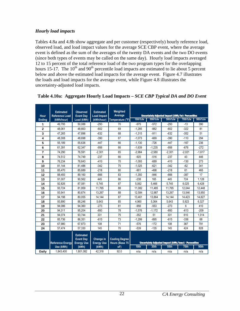
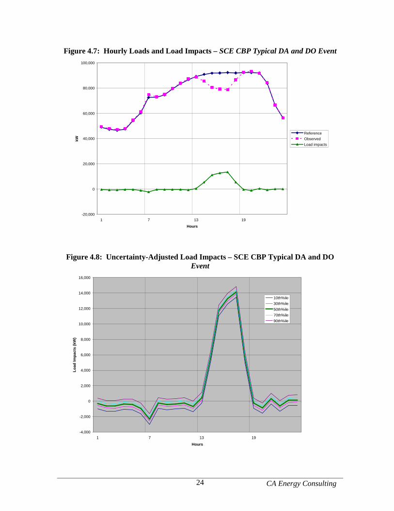
Hourly load impacts Tables 4.8a and 4.8b show aggregate and per customer (respectively) hourly reference load, observed load, and load impact values for the average SCE CBP event, where the average event is defined as the sum of the averages of the twenty DA events and the two DO events (since both types of events may be called on the same day). Hourly load impacts averaged 12 to 15 percent of the total reference load of the two program types for the overlapping hours 15-17. The 10th and 90th percentile load impacts are estimated to lie about 5 percent below and above the estimated load impacts for the average event. Figure 4.7 illustrates the loads and load impacts for the average event, while Figure 4.8 illustrates the uncertainty-adjusted load impacts. Table 4.10a: Aggregate Hourly Load Impacts – SCE CBP Typical DA and DO Event
Uncertainty Adjusted Impact (kWh/hr)- PercentilesUncertainty Adjusted Impact (kWh/hr)- PercentilesUncertainty Adjusted Impact (kWh/hr)- PercentilesUncertainty Adjusted Impact (kWh/hr)- Percentiles
10th%ile 30th%ile 50th%ile 70th%ile 90th%ile
1 49,795 50,088 -293 70 -975 -572 -293 -13 390
2 48,061 48,663 -602 69 -1,285 -882 -602 -322 81
3 47,265 47,896 -632 68 -1,315 -911 -632 -352 51
4 48,308 48,698 -390 67 -1,073 -669 -390 -110 294
5 55,189 55,636 -447 66 -1,130 -726 -447 -167 236
6 61,391 62,347 -956 66 -1,639 -1,235 -956 -676 -272
7 74,290 76,591 -2,301 65 -2,984 -2,580 -2,301 -2,021 -1,617
8 74,512 74,749 -237 66 -920 -516 -237 43 446
9 76,234 76,643 -410 70 -1,093 -689 -410 -130 273
10 81,144 81,486 -342 75 -1,025 -621 -342 -62 341
11 85,470 85,689 -218 80 -901 -498 -218 61 465
12 88,493 89,160 -666 83 -1,350 -946 -666 -387 17
13 91,007 90,562 445 86 -238 165 445 724 1,128
14 92,826 87,081 5,745 87 5,062 5,466 5,745 6,025 6,428
15 93,724 81,959 11,765 88 11,082 11,485 11,765 12,044 12,448
16 93,941 80,674 13,267 88 12,584 12,987 13,267 13,546 13,950
17 94,198 80,055 14,144 87 13,461 13,864 14,144 14,423 14,827
18 93,890 88,246 5,643 85 4,960 5,364 5,643 5,923 6,327
19 94,086 94,360 -273 81 -956 -553 -273 6 410
20 94,311 95,204 -893 78 -1,576 -1,172 -893 -613 -209
21 94,074 93,744 331 75 -352 51 331 610 1,014
22 85,736 86,351 -615 73 -1,299 -895 -615 -336 68
23 67,980 67,873 108 71 -576 -172 108 387 791
24 57,474 57,330 145 70 -539 -135 145 424 828
Uncertainty Adjusted Impact (kWh/hour) - PercentilesUncertainty Adjusted Impact (kWh/hour) - PercentilesUncertainty Adjusted Impact (kWh/hour) - PercentilesUncertainty Adjusted Impact (kWh/hour) - Percentiles
10th 30th 50th 70th 90th
Daily 1,843,400 1,801,082 42,318 92.0 n/a n/a n/a n/a n/a
Weighted
Average
Temperature (oF)
Reference Energy
Use (kWh)
Estimated
Event Day
Energy Use
(kWh)
Change in
Energy Use
(kWh)
Cooling Degree
Hours (Base 75
oF)
Hour
Ending
Estimated
Reference Load
(kWh/hour)
Observed
Event Day
Load (kWh)
Estimated
Load Impact
(kWh/hour)

CA Energy Consulting 23
Table 4.11b: Per Customer Hourly Load Impacts – SCE CBP Typical DA and DO Event
Uncertainty Adjusted Impact (kWh/hr)- PercentilesUncertainty Adjusted Impact (kWh/hr)- PercentilesUncertainty Adjusted Impact (kWh/hr)- PercentilesUncertainty Adjusted Impact (kWh/hr)- Percentiles
10th%ile 30th%ile 50th%ile 70th%ile 90th%ile
1 151 152 -1 70 -3 -2 -1 0 1
2 146 148 -2 69 -4 -3 -2 -1 0
3 144 145 -2 68 -4 -3 -2 -1 0
4 147 148 -1 67 -3 -2 -1 0 1
5 168 169 -1 66 -3 -2 -1 -1 1
6 186 189 -3 66 -5 -4 -3 -2 -1
7 226 233 -7 65 -9 -8 -7 -6 -5
8 226 227 -1 66 -3 -2 -1 0 1
9 232 233 -1 70 -3 -2 -1 0 1
10 246 247 -1 75 -3 -2 -1 0 1
11 260 260 -1 80 -3 -2 -1 0 1
12 269 271 -2 83 -4 -3 -2 -1 0
13 276 275 1 86 -1 1 1 2 3
14 282 264 17 87 15 17 17 18 20
15 285 249 36 88 34 35 36 37 38
16 285 245 40 88 38 39 40 41 42
17 286 243 43 87 41 42 43 44 45
18 285 268 17 85 15 16 17 18 19
19 286 287 -1 81 -3 -2 -1 0 1
20 286 289 -3 78 -5 -4 -3 -2 -1
21 286 285 1 75 -1 0 1 2 3
22 260 262 -2 73 -4 -3 -2 -1 0
23 206 206 0 71 -2 -1 0 1 2
24 175 174 0 70 -2 0 0 1 3
Uncertainty Adjusted Impact (kWh/hour) - PercentilesUncertainty Adjusted Impact (kWh/hour) - PercentilesUncertainty Adjusted Impact (kWh/hour) - PercentilesUncertainty Adjusted Impact (kWh/hour) - Percentiles
10th 30th 50th 70th 90th
Daily 5,598 5,470 129 92.0 n/a n/a n/a n/a n/a
Weighted
Average
Temperature (oF)
Reference Energy
Use (kWh)
Estimated
Event Day
Energy Use
(kWh)
Change in
Energy Use
(kWh)
Cooling Degree
Hours (Base 75
oF)
Hour
Ending
Estimated
Reference Load
(kWh/hour)
Observed
Event Day
Load (kWh)
Estimated
Load Impact
(kWh/hour)
CA Energy Consulting 24
Figure 4.7: Hourly Loads and Load Impacts – SCE CBP Typical DA and DO Event
-20,000
0
20,000
40,000
60,000
80,000
100,000
1 7 13 19
Hours
kW
Reference
Observed
Load impacts
Figure 4.8: Uncertainty-Adjusted Load Impacts – SCE CBP Typical DA and DO Event
-4,000
-2,000
0
2,000
4,000
6,000
8,000
10,000
12,000
14,000
16,000
1 7 13 19
Hours
Load
Impa
cts
(kW
)
10th%ile
30th%ile
50th%ile
70th%ile
90th%ile
CA Energy Consulting 25
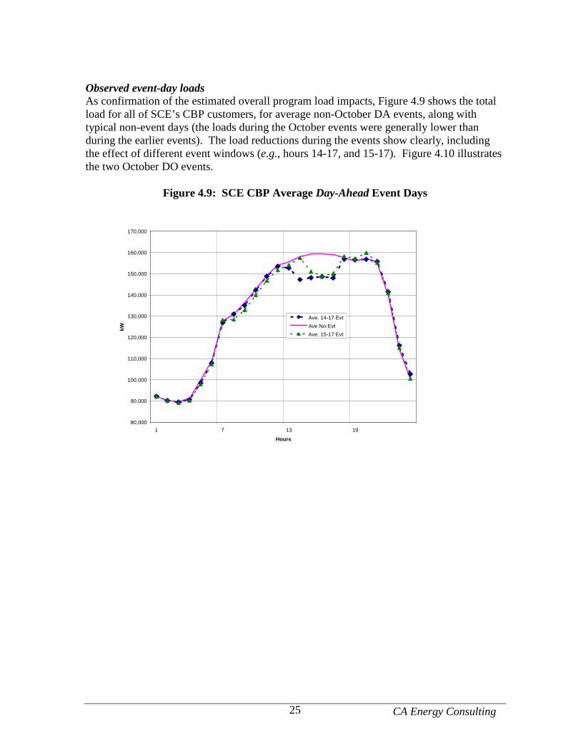
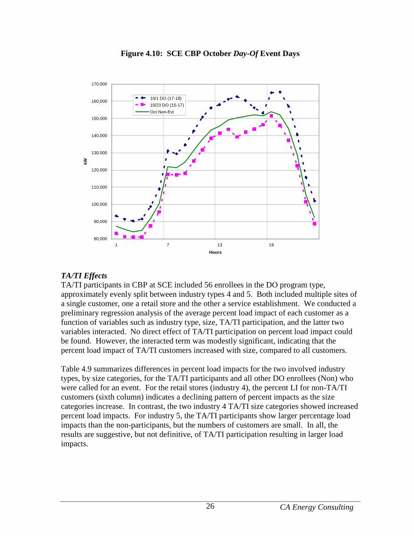
Observed event-day loads As confirmation of the estimated overall program load impacts, Figure 4.9 shows the total load for all of SCE’s CBP customers, for average non-October DA events, along with typical non-event days (the loads during the October events were generally lower than during the earlier events). The load reductions during the events show clearly, including the effect of different event windows (e.g., hours 14-17, and 15-17). Figure 4.10 illustrates the two October DO events.
Figure 4.9: SCE CBP Average Day-Ahead Event Days
80,000
90,000
100,000
110,000
120,000
130,000
140,000
150,000
160,000
170,000
1 7 13 19
Hours
kW
Ave. 14-17 Evt
Ave No-Evt
Ave. 15-17 Evt
CA Energy Consulting 26
Figure 4.10: SCE CBP October Day-Of Event Days
80,000
90,000
100,000
110,000
120,000
130,000
140,000
150,000
160,000
170,000
1 7 13 19
Hours
kW
10/1 DO (17-18)
10/23 DO (15-17)
Oct Non-Evt
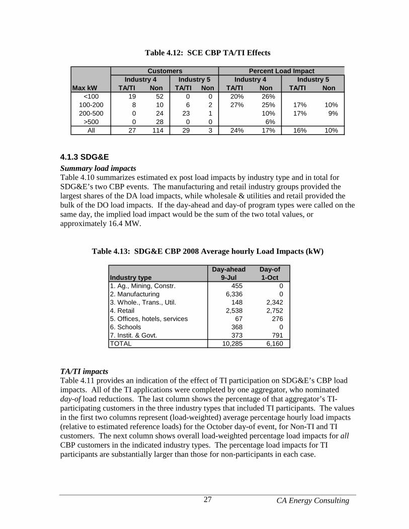
TA/TI Effects TA/TI participants in CBP at SCE included 56 enrollees in the DO program type, approximately evenly split between industry types 4 and 5. Both included multiple sites of a single customer, one a retail store and the other a service establishment. We conducted a preliminary regression analysis of the average percent load impact of each customer as a function of variables such as industry type, size, TA/TI participation, and the latter two variables interacted. No direct effect of TA/TI participation on percent load impact could be found. However, the interacted term was modestly significant, indicating that the percent load impact of TA/TI customers increased with size, compared to all customers. Table 4.9 summarizes differences in percent load impacts for the two involved industry types, by size categories, for the TA/TI participants and all other DO enrollees (Non) who were called for an event. For the retail stores (industry 4), the percent LI for non-TA/TI customers (sixth column) indicates a declining pattern of percent impacts as the size categories increase. In contrast, the two industry 4 TA/TI size categories showed increased percent load impacts. For industry 5, the TA/TI participants show larger percentage load impacts than the non-participants, but the numbers of customers are small. In all, the results are suggestive, but not definitive, of TA/TI participation resulting in larger load impacts.
CA Energy Consulting 27
Table 4.12: SCE CBP TA/TI Effects
Max kW TA/TI Non TA/TI Non TA/TI Non TA/TI Non<100 19 52 0 0 20% 26%
100-200 8 10 6 2 27% 25% 17% 10%200-500 0 24 23 1 10% 17% 9%
>500 0 28 0 0 6%All 27 114 29 3 24% 17% 16% 10%
Percent Load ImpactCustomersIndustry 4 Industry 5 Industry 4 Industry 5
4.1.3 SDG&E Summary load impacts Table 4.10 summarizes estimated ex post load impacts by industry type and in total for SDG&E’s two CBP events. The manufacturing and retail industry groups provided the largest shares of the DA load impacts, while wholesale & utilities and retail provided the bulk of the DO load impacts. If the day-ahead and day-of program types were called on the same day, the implied load impact would be the sum of the two total values, or approximately 16.4 MW.
Table 4.13: SDG&E CBP 2008 Average hourly Load Impacts (kW)
Day-ahead Day-of
Industry type 9-Jul 1-Oct1. Ag., Mining, Constr. 455 02. Manufacturing 6,336 03. Whole., Trans., Util. 148 2,3424. Retail 2,538 2,7525. Offices, hotels, services 67 2766. Schools 368 07. Instit. & Govt. 373 791TOTAL 10,285 6,160
TA/TI impacts Table 4.11 provides an indication of the effect of TI participation on SDG&E’s CBP load impacts. All of the TI applications were completed by one aggregator, who nominated day-of load reductions. The last column shows the percentage of that aggregator’s TI-participating customers in the three industry types that included TI participants. The values in the first two columns represent (load-weighted) average percentage hourly load impacts (relative to estimated reference loads) for the October day-of event, for Non-TI and TI customers. The next column shows overall load-weighted percentage load impacts for all CBP customers in the indicated industry types. The percentage load impacts for TI participants are substantially larger than those for non-participants in each case.
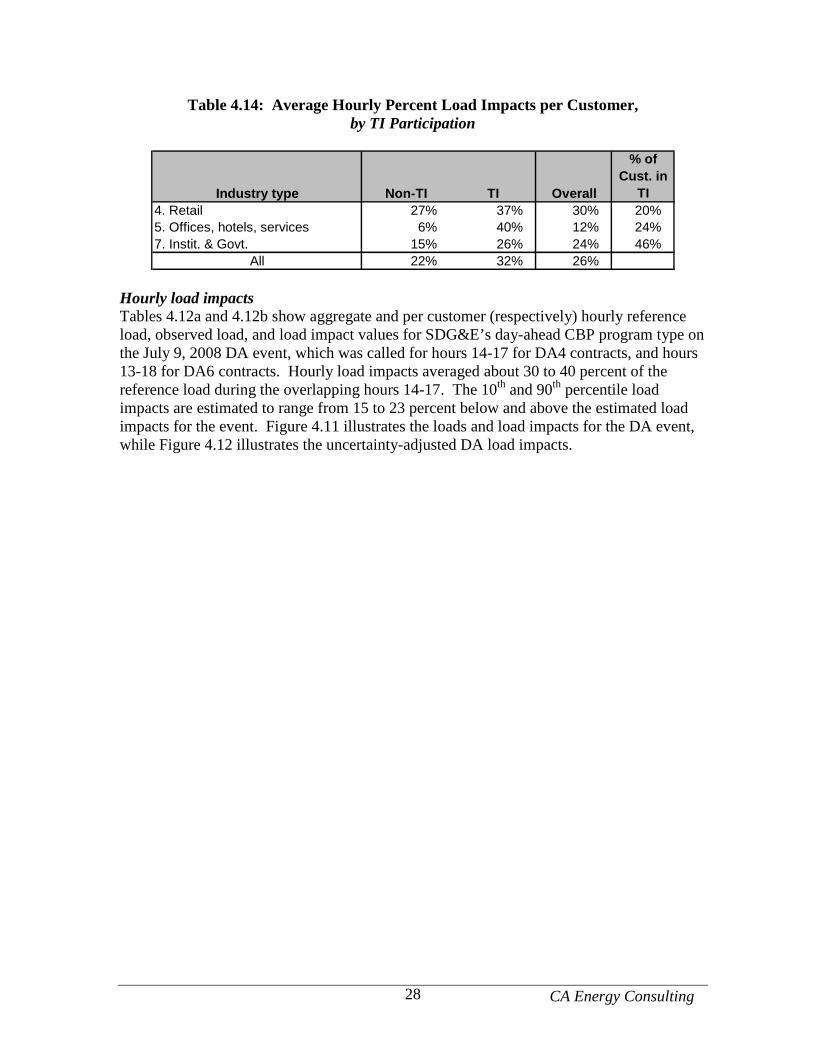
CA Energy Consulting 28
Table 4.14: Average Hourly Percent Load Impacts per Customer, by TI Participation
Industry type Non-TI TI Overall
% of Cust. in
TI4. Retail 27% 37% 30% 20%5. Offices, hotels, services 6% 40% 12% 24%7. Instit. & Govt. 15% 26% 24% 46%
All 22% 32% 26% Hourly load impacts Tables 4.12a and 4.12b show aggregate and per customer (respectively) hourly reference load, observed load, and load impact values for SDG&E’s day-ahead CBP program type on the July 9, 2008 DA event, which was called for hours 14-17 for DA4 contracts, and hours 13-18 for DA6 contracts. Hourly load impacts averaged about 30 to 40 percent of the reference load during the overlapping hours 14-17. The 10th and 90th percentile load impacts are estimated to range from 15 to 23 percent below and above the estimated load impacts for the event. Figure 4.11 illustrates the loads and load impacts for the DA event, while Figure 4.12 illustrates the uncertainty-adjusted DA load impacts.
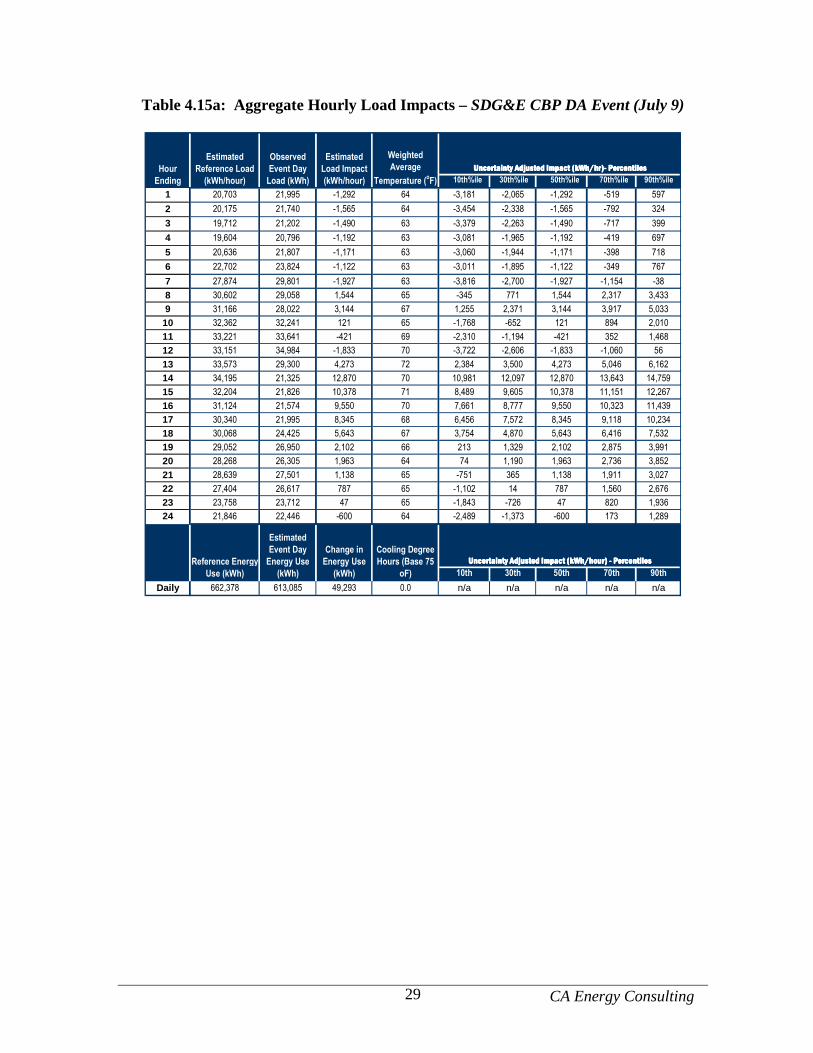
CA Energy Consulting 29
Table 4.15a: Aggregate Hourly Load Impacts – SDG&E CBP DA Event (July 9)
Uncertainty Adjusted Impact (kWh/hr)- PercentilesUncertainty Adjusted Impact (kWh/hr)- PercentilesUncertainty Adjusted Impact (kWh/hr)- PercentilesUncertainty Adjusted Impact (kWh/hr)- Percentiles
10th%ile 30th%ile 50th%ile 70th%ile 90th%ile
1 20,703 21,995 -1,292 64 -3,181 -2,065 -1,292 -519 597
2 20,175 21,740 -1,565 64 -3,454 -2,338 -1,565 -792 324
3 19,712 21,202 -1,490 63 -3,379 -2,263 -1,490 -717 399
4 19,604 20,796 -1,192 63 -3,081 -1,965 -1,192 -419 697
5 20,636 21,807 -1,171 63 -3,060 -1,944 -1,171 -398 718
6 22,702 23,824 -1,122 63 -3,011 -1,895 -1,122 -349 767
7 27,874 29,801 -1,927 63 -3,816 -2,700 -1,927 -1,154 -38
8 30,602 29,058 1,544 65 -345 771 1,544 2,317 3,433
9 31,166 28,022 3,144 67 1,255 2,371 3,144 3,917 5,033
10 32,362 32,241 121 65 -1,768 -652 121 894 2,010
11 33,221 33,641 -421 69 -2,310 -1,194 -421 352 1,468
12 33,151 34,984 -1,833 70 -3,722 -2,606 -1,833 -1,060 56
13 33,573 29,300 4,273 72 2,384 3,500 4,273 5,046 6,162
14 34,195 21,325 12,870 70 10,981 12,097 12,870 13,643 14,759
15 32,204 21,826 10,378 71 8,489 9,605 10,378 11,151 12,267
16 31,124 21,574 9,550 70 7,661 8,777 9,550 10,323 11,439
17 30,340 21,995 8,345 68 6,456 7,572 8,345 9,118 10,234
18 30,068 24,425 5,643 67 3,754 4,870 5,643 6,416 7,532
19 29,052 26,950 2,102 66 213 1,329 2,102 2,875 3,991
20 28,268 26,305 1,963 64 74 1,190 1,963 2,736 3,852
21 28,639 27,501 1,138 65 -751 365 1,138 1,911 3,027
22 27,404 26,617 787 65 -1,102 14 787 1,560 2,676
23 23,758 23,712 47 65 -1,843 -726 47 820 1,936
24 21,846 22,446 -600 64 -2,489 -1,373 -600 173 1,289
Uncertainty Adjusted Impact (kWh/hour) - PercentilesUncertainty Adjusted Impact (kWh/hour) - PercentilesUncertainty Adjusted Impact (kWh/hour) - PercentilesUncertainty Adjusted Impact (kWh/hour) - Percentiles
10th 30th 50th 70th 90th
Daily 662,378 613,085 49,293 0.0 n/a n/a n/a n/a n/a
Hour
Ending
Estimated
Reference Load
(kWh/hour)
Observed
Event Day
Load (kWh)
Estimated
Load Impact
(kWh/hour)
Weighted
Average
Temperature (oF)
Reference Energy
Use (kWh)
Estimated
Event Day
Energy Use
(kWh)
Change in
Energy Use
(kWh)
Cooling Degree
Hours (Base 75
oF)
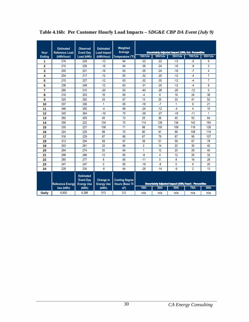
CA Energy Consulting 30
Table 4.16b: Per Customer Hourly Load Impacts – SDG&E CBP DA Event (July 9)
Uncertainty Adjusted Impact (kWh/hr)- PercentilesUncertainty Adjusted Impact (kWh/hr)- PercentilesUncertainty Adjusted Impact (kWh/hr)- PercentilesUncertainty Adjusted Impact (kWh/hr)- Percentiles
10th%ile 30th%ile 50th%ile 70th%ile 90th%ile
1 216 229 -13 64 -33 -22 -13 -5 6
2 210 226 -16 64 -36 -24 -16 -8 3
3 205 221 -16 63 -35 -24 -16 -7 4
4 204 217 -12 63 -32 -20 -12 -4 7
5 215 227 -12 63 -32 -20 -12 -4 7
6 236 248 -12 63 -31 -20 -12 -4 8
7 290 310 -20 63 -40 -28 -20 -12 0
8 319 303 16 65 -4 8 16 24 36
9 325 292 33 67 13 25 33 41 52
10 337 336 1 65 -18 -7 1 9 21
11 346 350 -4 69 -24 -12 -4 4 15
12 345 364 -19 70 -39 -27 -19 -11 1
13 350 305 45 72 25 36 45 53 64
14 356 222 134 70 114 126 134 142 154
15 335 227 108 71 88 100 108 116 128
16 324 225 99 70 80 91 99 108 119
17 316 229 87 68 67 79 87 95 107
18 313 254 59 67 39 51 59 67 78
19 303 281 22 66 2 14 22 30 42
20 294 274 20 64 1 12 20 29 40
21 298 286 12 65 -8 4 12 20 32
22 285 277 8 65 -11 0 8 16 28
23 247 247 0 65 -19 -8 0 9 20
24 228 234 -6 64 -26 -14 -6 2 13
Uncertainty Adjusted Impact (kWh/hour) - PercentilesUncertainty Adjusted Impact (kWh/hour) - PercentilesUncertainty Adjusted Impact (kWh/hour) - PercentilesUncertainty Adjusted Impact (kWh/hour) - Percentiles
10th 30th 50th 70th 90th
Daily 6,900 6,386 513 0.0 n/a n/a n/a n/a n/a
Weighted
Average
Temperature (oF)
Reference Energy
Use (kWh)
Estimated
Event Day
Energy Use
(kWh)
Change in
Energy Use
(kWh)
Cooling Degree
Hours (Base 75
oF)
Hour
Ending
Estimated
Reference Load
(kWh/hour)
Observed
Event Day
Load (kWh)
Estimated
Load Impact
(kWh/hour)
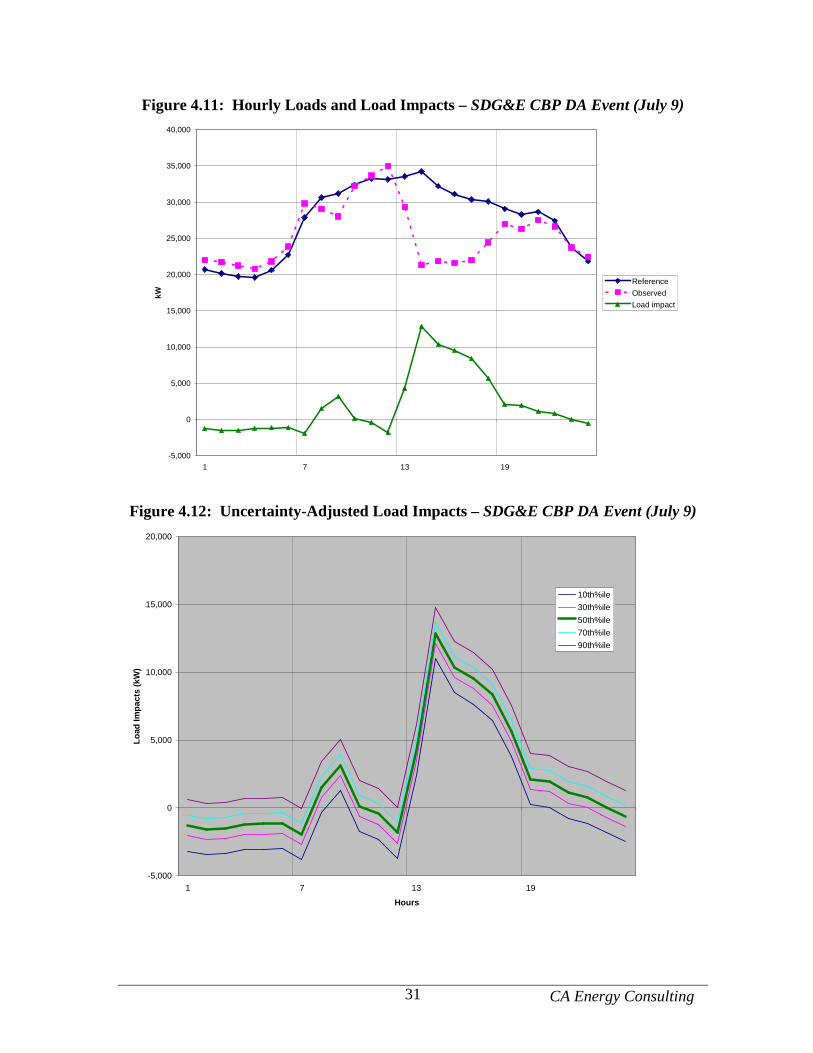
CA Energy Consulting 31
Figure 4.11: Hourly Loads and Load Impacts – SDG&E CBP DA Event (July 9)
-5,000
0
5,000
10,000
15,000
20,000
25,000
30,000
35,000
40,000
1 7 13 19
kW
Reference
Observed
Load impact
Figure 4.12: Uncertainty-Adjusted Load Impacts – SDG&E CBP DA Event (July 9)
-5,000
0
5,000
10,000
15,000
20,000
1 7 13 19
Hours
Load
Impa
cts
(kW
)
10th%ile
30th%ile
50th%ile
70th%ile
90th%ile
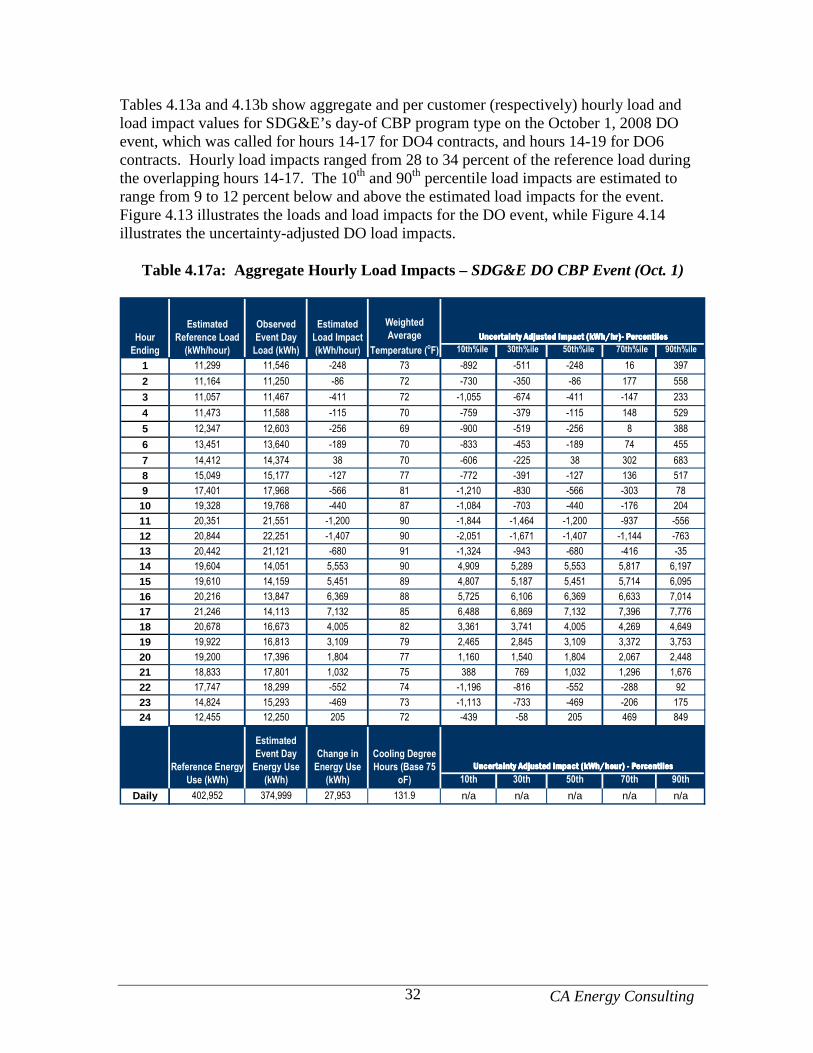
CA Energy Consulting 32
Tables 4.13a and 4.13b show aggregate and per customer (respectively) hourly load and load impact values for SDG&E’s day-of CBP program type on the October 1, 2008 DO event, which was called for hours 14-17 for DO4 contracts, and hours 14-19 for DO6 contracts. Hourly load impacts ranged from 28 to 34 percent of the reference load during the overlapping hours 14-17. The 10th and 90th percentile load impacts are estimated to range from 9 to 12 percent below and above the estimated load impacts for the event. Figure 4.13 illustrates the loads and load impacts for the DO event, while Figure 4.14 illustrates the uncertainty-adjusted DO load impacts.
Table 4.17a: Aggregate Hourly Load Impacts – SDG&E DO CBP Event (Oct. 1)
Uncertainty Adjusted Impact (kWh/hr)- PercentilesUncertainty Adjusted Impact (kWh/hr)- PercentilesUncertainty Adjusted Impact (kWh/hr)- PercentilesUncertainty Adjusted Impact (kWh/hr)- Percentiles
10th%ile 30th%ile 50th%ile 70th%ile 90th%ile
1 11,299 11,546 -248 73 -892 -511 -248 16 397
2 11,164 11,250 -86 72 -730 -350 -86 177 558
3 11,057 11,467 -411 72 -1,055 -674 -411 -147 233
4 11,473 11,588 -115 70 -759 -379 -115 148 529
5 12,347 12,603 -256 69 -900 -519 -256 8 388
6 13,451 13,640 -189 70 -833 -453 -189 74 455
7 14,412 14,374 38 70 -606 -225 38 302 683
8 15,049 15,177 -127 77 -772 -391 -127 136 517
9 17,401 17,968 -566 81 -1,210 -830 -566 -303 78
10 19,328 19,768 -440 87 -1,084 -703 -440 -176 204
11 20,351 21,551 -1,200 90 -1,844 -1,464 -1,200 -937 -556
12 20,844 22,251 -1,407 90 -2,051 -1,671 -1,407 -1,144 -763
13 20,442 21,121 -680 91 -1,324 -943 -680 -416 -35
14 19,604 14,051 5,553 90 4,909 5,289 5,553 5,817 6,197
15 19,610 14,159 5,451 89 4,807 5,187 5,451 5,714 6,095
16 20,216 13,847 6,369 88 5,725 6,106 6,369 6,633 7,014
17 21,246 14,113 7,132 85 6,488 6,869 7,132 7,396 7,776
18 20,678 16,673 4,005 82 3,361 3,741 4,005 4,269 4,649
19 19,922 16,813 3,109 79 2,465 2,845 3,109 3,372 3,753
20 19,200 17,396 1,804 77 1,160 1,540 1,804 2,067 2,448
21 18,833 17,801 1,032 75 388 769 1,032 1,296 1,676
22 17,747 18,299 -552 74 -1,196 -816 -552 -288 92
23 14,824 15,293 -469 73 -1,113 -733 -469 -206 175
24 12,455 12,250 205 72 -439 -58 205 469 849
Uncertainty Adjusted Impact (kWh/hour) - PercentilesUncertainty Adjusted Impact (kWh/hour) - PercentilesUncertainty Adjusted Impact (kWh/hour) - PercentilesUncertainty Adjusted Impact (kWh/hour) - Percentiles
10th 30th 50th 70th 90th
Daily 402,952 374,999 27,953 131.9 n/a n/a n/a n/a n/a
Hour
Ending
Estimated
Reference Load
(kWh/hour)
Observed
Event Day
Load (kWh)
Estimated
Load Impact
(kWh/hour)
Weighted
Average
Temperature (oF)
Reference Energy
Use (kWh)
Estimated
Event Day
Energy Use
(kWh)
Change in
Energy Use
(kWh)
Cooling Degree
Hours (Base 75
oF)
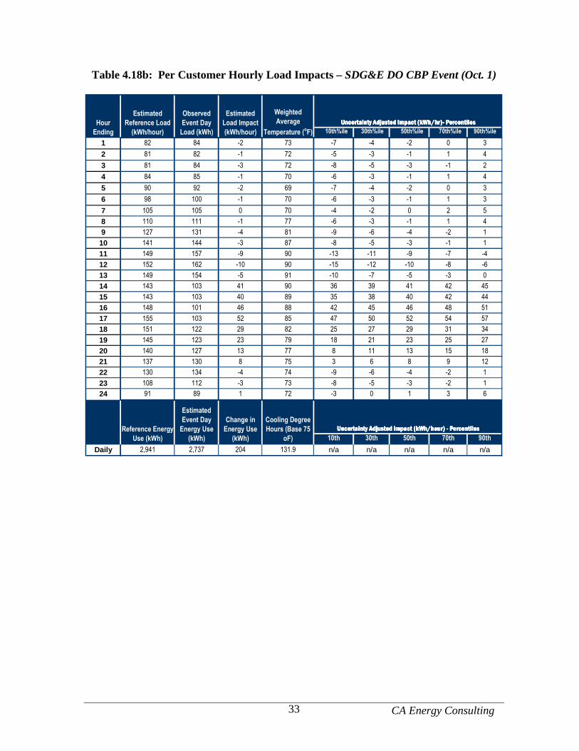
CA Energy Consulting 33
Table 4.18b: Per Customer Hourly Load Impacts – SDG&E DO CBP Event (Oct. 1)
Uncertainty Adjusted Impact (kWh/hr)- PercentilesUncertainty Adjusted Impact (kWh/hr)- PercentilesUncertainty Adjusted Impact (kWh/hr)- PercentilesUncertainty Adjusted Impact (kWh/hr)- Percentiles
10th%ile 30th%ile 50th%ile 70th%ile 90th%ile
1 82 84 -2 73 -7 -4 -2 0 3
2 81 82 -1 72 -5 -3 -1 1 4
3 81 84 -3 72 -8 -5 -3 -1 2
4 84 85 -1 70 -6 -3 -1 1 4
5 90 92 -2 69 -7 -4 -2 0 3
6 98 100 -1 70 -6 -3 -1 1 3
7 105 105 0 70 -4 -2 0 2 5
8 110 111 -1 77 -6 -3 -1 1 4
9 127 131 -4 81 -9 -6 -4 -2 1
10 141 144 -3 87 -8 -5 -3 -1 1
11 149 157 -9 90 -13 -11 -9 -7 -4
12 152 162 -10 90 -15 -12 -10 -8 -6
13 149 154 -5 91 -10 -7 -5 -3 0
14 143 103 41 90 36 39 41 42 45
15 143 103 40 89 35 38 40 42 44
16 148 101 46 88 42 45 46 48 51
17 155 103 52 85 47 50 52 54 57
18 151 122 29 82 25 27 29 31 34
19 145 123 23 79 18 21 23 25 27
20 140 127 13 77 8 11 13 15 18
21 137 130 8 75 3 6 8 9 12
22 130 134 -4 74 -9 -6 -4 -2 1
23 108 112 -3 73 -8 -5 -3 -2 1
24 91 89 1 72 -3 0 1 3 6
Uncertainty Adjusted Impact (kWh/hour) - PercentilesUncertainty Adjusted Impact (kWh/hour) - PercentilesUncertainty Adjusted Impact (kWh/hour) - PercentilesUncertainty Adjusted Impact (kWh/hour) - Percentiles
10th 30th 50th 70th 90th
Daily 2,941 2,737 204 131.9 n/a n/a n/a n/a n/a
Weighted
Average
Temperature (oF)
Reference Energy
Use (kWh)
Estimated
Event Day
Energy Use
(kWh)
Change in
Energy Use
(kWh)
Cooling Degree
Hours (Base 75
oF)
Hour
Ending
Estimated
Reference Load
(kWh/hour)
Observed
Event Day
Load (kWh)
Estimated
Load Impact
(kWh/hour)
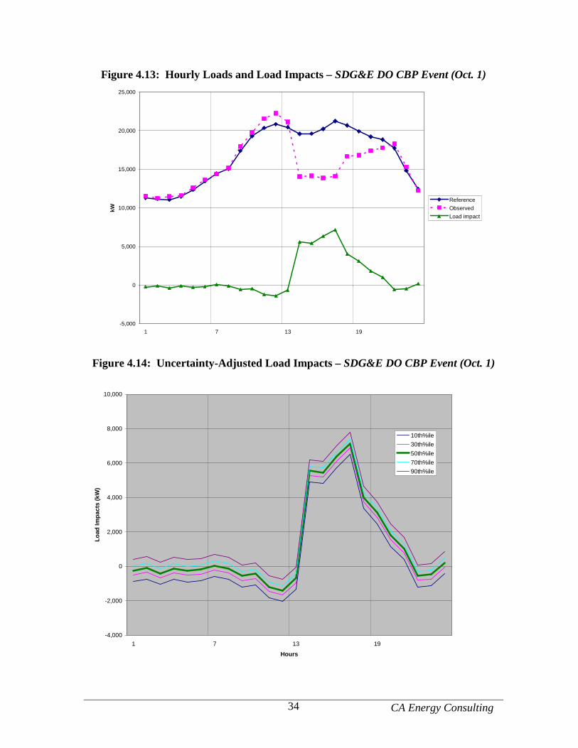
CA Energy Consulting 34
Figure 4.13: Hourly Loads and Load Impacts – SDG&E DO CBP Event (Oct. 1)
-5,000
0
5,000
10,000
15,000
20,000
25,000
1 7 13 19
kW
Reference
Observed
Load impact
Figure 4.14: Uncertainty-Adjusted Load Impacts – SDG&E DO CBP Event (Oct. 1)
-4,000
-2,000
0
2,000
4,000
6,000
8,000
10,000
1 7 13 19
Hours
Load
Impa
cts
(kW
)
10th%ile
30th%ile
50th%ile
70th%ile
90th%ile
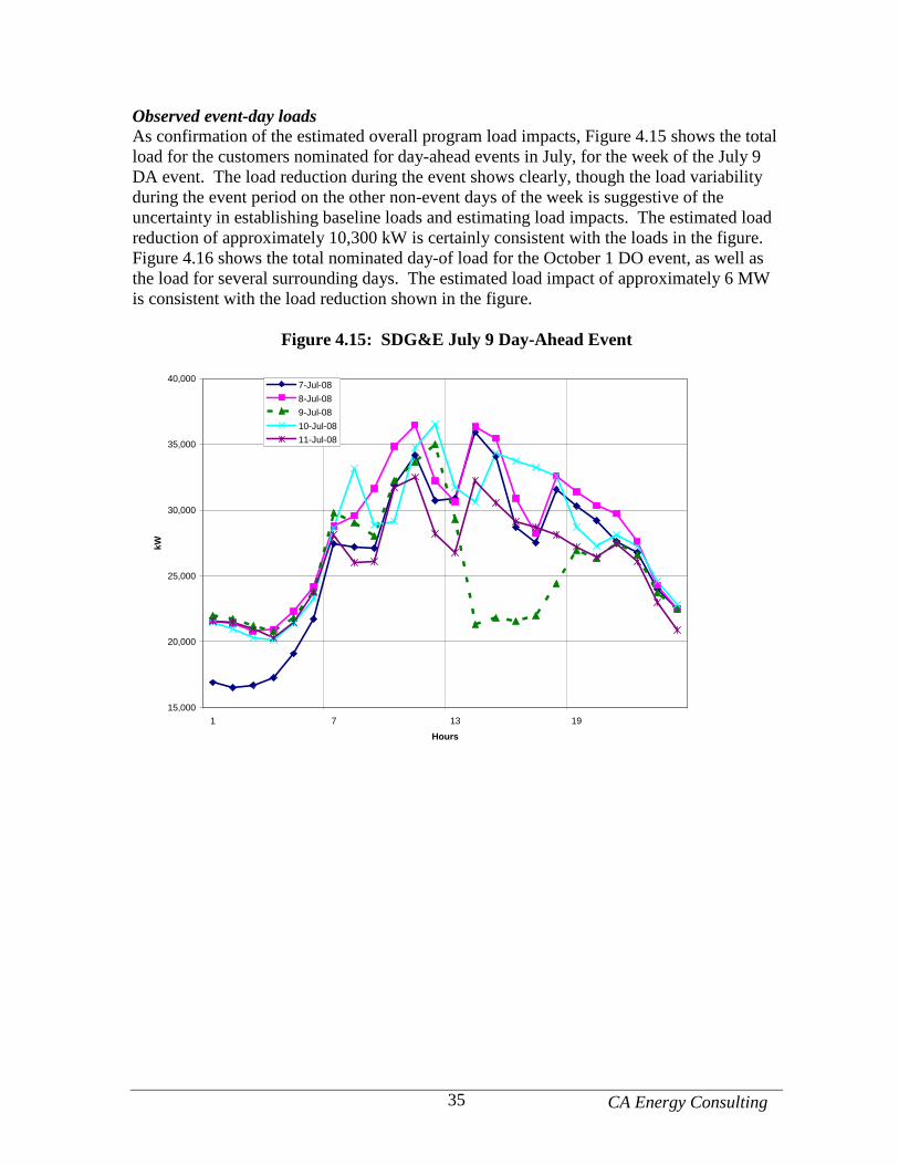
CA Energy Consulting 35
Observed event-day loads As confirmation of the estimated overall program load impacts, Figure 4.15 shows the total load for the customers nominated for day-ahead events in July, for the week of the July 9 DA event. The load reduction during the event shows clearly, though the load variability during the event period on the other non-event days of the week is suggestive of the uncertainty in establishing baseline loads and estimating load impacts. The estimated load reduction of approximately 10,300 kW is certainly consistent with the loads in the figure. Figure 4.16 shows the total nominated day-of load for the October 1 DO event, as well as the load for several surrounding days. The estimated load impact of approximately 6 MW is consistent with the load reduction shown in the figure.
Figure 4.15: SDG&E July 9 Day-Ahead Event
15,000
20,000
25,000
30,000
35,000
40,000
1 7 13 19
Hours
kW
7-Jul-08
8-Jul-08
9-Jul-08
10-Jul-08
11-Jul-08
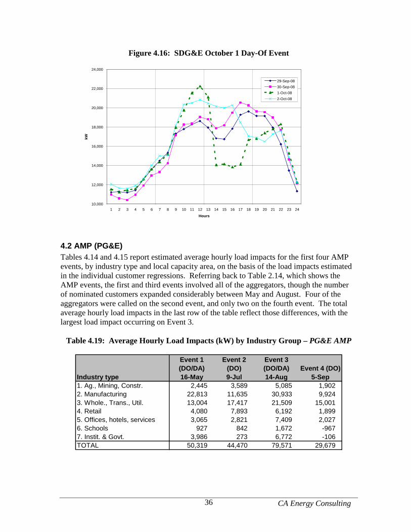
CA Energy Consulting 36
Figure 4.16: SDG&E October 1 Day-Of Event
10,000
12,000
14,000
16,000
18,000
20,000
22,000
24,000
1 2 3 4 5 6 7 8 9 10 11 12 13 14 15 16 17 18 19 20 21 22 23 24
Hours
kW29-Sep-08
30-Sep-08
1-Oct-08
2-Oct-08
4.2 AMP (PG&E) Tables 4.14 and 4.15 report estimated average hourly load impacts for the first four AMP events, by industry type and local capacity area, on the basis of the load impacts estimated in the individual customer regressions. Referring back to Table 2.14, which shows the AMP events, the first and third events involved all of the aggregators, though the number of nominated customers expanded considerably between May and August. Four of the aggregators were called on the second event, and only two on the fourth event. The total average hourly load impacts in the last row of the table reflect those differences, with the largest load impact occurring on Event 3.
Table 4.19: Average Hourly Load Impacts (kW) by Industry Group – PG&E AMP
Event 1 (DO/DA)
Event 2 (DO)
Event 3 (DO/DA) Event 4 (DO)
Industry type 16-May 9-Jul 14-Aug 5-Sep1. Ag., Mining, Constr. 2,445 3,589 5,085 1,9022. Manufacturing 22,813 11,635 30,933 9,9243. Whole., Trans., Util. 13,004 17,417 21,509 15,0014. Retail 4,080 7,893 6,192 1,8995. Offices, hotels, services 3,065 2,821 7,409 2,0276. Schools 927 842 1,672 -9677. Instit. & Govt. 3,986 273 6,772 -106TOTAL 50,319 44,470 79,571 29,679
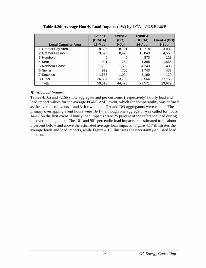
CA Energy Consulting 37
Table 4.20: Average Hourly Load Impacts (kW) by LCA – PG&E AMP
Event 1 (DO/DA)
Event 2 (DO)
Event 3 (DO/DA) Event 4 (DO)
Local Capacity Area 16-May 9-Jul 14-Aug 5-Sep1 Greater Bay Area 8,605 8,191 12,718 4,8322 Greater Fresno 9,528 8,476 16,843 4,5533 Humboldt 0 0 873 1184 Kern 1,091 750 1,388 1,6655 Northern Coast 1,700 1,585 4,243 4086 Sierra 972 705 1,743 4777 Stockton 1,535 1,024 3,199 -1298 Other 26,887 23,739 38,564 17,756
Total 50,319 44,470 79,571 29,679 Hourly load impacts Tables 4.16a and 4.16b show aggregate and per customer (respectively) hourly load and load impact values for the average PG&E AMP event, which for comparability was defined as the average of events 1 and 3, for which all DA and DO aggregators were called. The primary overlapping event hours were 16-17, although one aggregator was called for hours 14-17 on the first event. Hourly load impacts were 25 percent of the reference load during the overlapping hours. The 10th and 90th percentile load impacts are estimated to lie about 5 percent below and above the estimated average load impacts. Figure 4.17 illustrates the average loads and load impacts, while Figure 4.18 illustrates the uncertainty-adjusted load impacts.
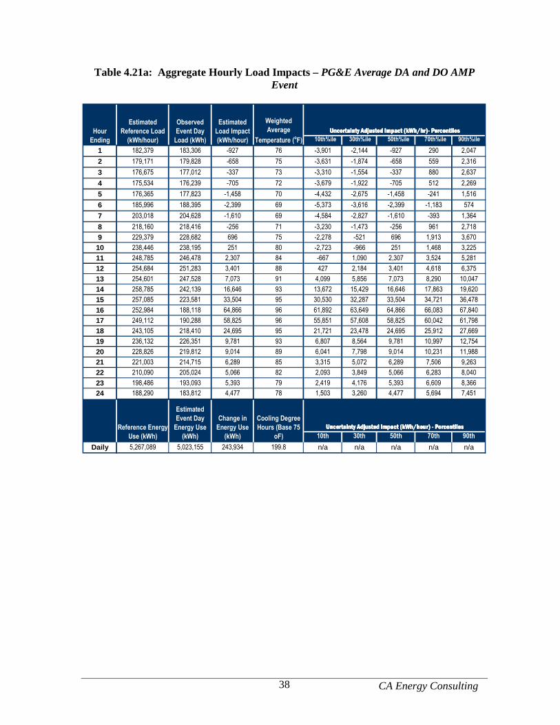
CA Energy Consulting 38
Table 4.21a: Aggregate Hourly Load Impacts – PG&E Average DA and DO AMP Event
Uncertainty Adjusted Impact (kWh/hr)- PercentilesUncertainty Adjusted Impact (kWh/hr)- PercentilesUncertainty Adjusted Impact (kWh/hr)- PercentilesUncertainty Adjusted Impact (kWh/hr)- Percentiles
10th%ile 30th%ile 50th%ile 70th%ile 90th%ile
1 182,379 183,306 -927 76 -3,901 -2,144 -927 290 2,047
2 179,171 179,828 -658 75 -3,631 -1,874 -658 559 2,316
3 176,675 177,012 -337 73 -3,310 -1,554 -337 880 2,637
4 175,534 176,239 -705 72 -3,679 -1,922 -705 512 2,269
5 176,365 177,823 -1,458 70 -4,432 -2,675 -1,458 -241 1,516
6 185,996 188,395 -2,399 69 -5,373 -3,616 -2,399 -1,183 574
7 203,018 204,628 -1,610 69 -4,584 -2,827 -1,610 -393 1,364
8 218,160 218,416 -256 71 -3,230 -1,473 -256 961 2,718
9 229,379 228,682 696 75 -2,278 -521 696 1,913 3,670
10 238,446 238,195 251 80 -2,723 -966 251 1,468 3,225
11 248,785 246,478 2,307 84 -667 1,090 2,307 3,524 5,281
12 254,684 251,283 3,401 88 427 2,184 3,401 4,618 6,375
13 254,601 247,528 7,073 91 4,099 5,856 7,073 8,290 10,047
14 258,785 242,139 16,646 93 13,672 15,429 16,646 17,863 19,620
15 257,085 223,581 33,504 95 30,530 32,287 33,504 34,721 36,478
16 252,984 188,118 64,866 96 61,892 63,649 64,866 66,083 67,840
17 249,112 190,288 58,825 96 55,851 57,608 58,825 60,042 61,798
18 243,105 218,410 24,695 95 21,721 23,478 24,695 25,912 27,669
19 236,132 226,351 9,781 93 6,807 8,564 9,781 10,997 12,754
20 228,826 219,812 9,014 89 6,041 7,798 9,014 10,231 11,988
21 221,003 214,715 6,289 85 3,315 5,072 6,289 7,506 9,263
22 210,090 205,024 5,066 82 2,093 3,849 5,066 6,283 8,040
23 198,486 193,093 5,393 79 2,419 4,176 5,393 6,609 8,366
24 188,290 183,812 4,477 78 1,503 3,260 4,477 5,694 7,451
Uncertainty Adjusted Impact (kWh/hour) - PercentilesUncertainty Adjusted Impact (kWh/hour) - PercentilesUncertainty Adjusted Impact (kWh/hour) - PercentilesUncertainty Adjusted Impact (kWh/hour) - Percentiles
10th 30th 50th 70th 90th
Daily 5,267,089 5,023,155 243,934 199.8 n/a n/a n/a n/a n/a
Weighted
Average
Temperature (oF)
Reference Energy
Use (kWh)
Estimated
Event Day
Energy Use
(kWh)
Change in
Energy Use
(kWh)
Cooling Degree
Hours (Base 75
oF)
Hour
Ending
Estimated
Reference Load
(kWh/hour)
Observed
Event Day
Load (kWh)
Estimated
Load Impact
(kWh/hour)

CA Energy Consulting 39
Table 4.22b: Per Customer Hourly Load Impacts – PG&E Average DA and DO AMP Event
Uncertainty Adjusted Impact (kWh/hr)- PercentilesUncertainty Adjusted Impact (kWh/hr)- PercentilesUncertainty Adjusted Impact (kWh/hr)- PercentilesUncertainty Adjusted Impact (kWh/hr)- Percentiles
10th%ile 30th%ile 50th%ile 70th%ile 90th%ile
1 493 495 -3 76 -11 -6 -3 1 6
2 484 486 -2 75 -10 -5 -2 2 6
3 478 478 -1 73 -9 -4 -1 2 7
4 474 476 -2 72 -10 -5 -2 1 6
5 477 481 -4 70 -12 -7 -4 -1 4
6 503 509 -6 69 -15 -10 -6 -3 2
7 549 553 -4 69 -12 -8 -4 -1 4
8 590 590 -1 71 -9 -4 -1 3 7
9 620 618 2 75 -6 -1 2 5 10
10 644 644 1 80 -7 -3 1 4 9
11 672 666 6 84 -2 3 6 10 14
12 688 679 9 88 1 6 9 12 17
13 688 669 19 91 11 16 19 22 27
14 699 654 45 93 37 42 45 48 53
15 695 604 91 95 83 87 91 94 99
16 684 508 175 96 167 172 175 179 183
17 673 514 159 96 151 156 159 162 167
18 657 590 67 95 59 63 67 70 75
19 638 612 26 93 18 23 26 30 34
20 618 594 24 89 16 21 24 28 32
21 597 580 17 85 9 14 17 20 25
22 568 554 14 82 6 10 14 17 22
23 536 522 15 79 7 11 15 18 23
24 509 497 12 78 4 9 12 15 20
Uncertainty Adjusted Impact (kWh/hour) - PercentilesUncertainty Adjusted Impact (kWh/hour) - PercentilesUncertainty Adjusted Impact (kWh/hour) - PercentilesUncertainty Adjusted Impact (kWh/hour) - Percentiles
10th 30th 50th 70th 90th
Daily 14,235 13,576 659 199.8 n/a n/a n/a n/a n/a
Hour
Ending
Estimated
Reference Load
(kWh/hour)
Observed
Event Day
Load (kWh)
Estimated
Load Impact
(kWh/hour)
Weighted
Average
Temperature (oF)
Reference Energy
Use (kWh)
Estimated
Event Day
Energy Use
(kWh)
Change in
Energy Use
(kWh)
Cooling Degree
Hours (Base 75
oF)
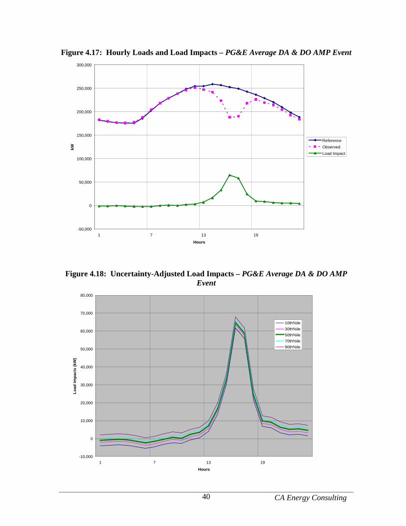
CA Energy Consulting 40
Figure 4.17: Hourly Loads and Load Impacts – PG&E Average DA & DO AMP Event
-50,000
0
50,000
100,000
150,000
200,000
250,000
300,000
1 7 13 19
Hours
kW
Reference
Observed
Load Impact
Figure 4.18: Uncertainty-Adjusted Load Impacts – PG&E Average DA & DO AMP Event
-10,000
0
10,000
20,000
30,000
40,000
50,000
60,000
70,000
80,000
1 7 13 19
Hours
Load
Impa
cts
(kW
)
10th%ile
30th%ile
50th%ile
70th%ile
90th%ile
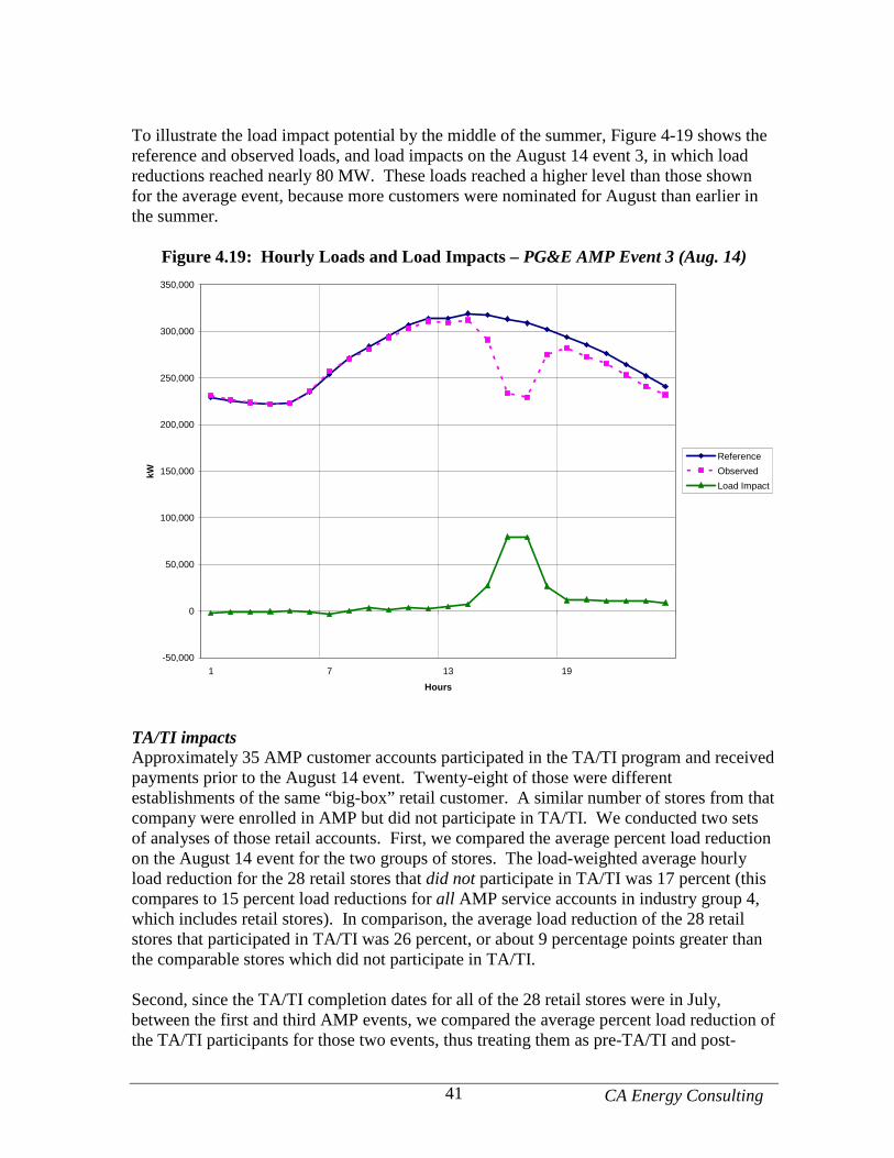
CA Energy Consulting 41
To illustrate the load impact potential by the middle of the summer, Figure 4-19 shows the reference and observed loads, and load impacts on the August 14 event 3, in which load reductions reached nearly 80 MW. These loads reached a higher level than those shown for the average event, because more customers were nominated for August than earlier in the summer.
Figure 4.19: Hourly Loads and Load Impacts – PG&E AMP Event 3 (Aug. 14)
-50,000
0
50,000
100,000
150,000
200,000
250,000
300,000
350,000
1 7 13 19
Hours
kW
Reference
Observed
Load Impact
TA/TI impacts Approximately 35 AMP customer accounts participated in the TA/TI program and received payments prior to the August 14 event. Twenty-eight of those were different establishments of the same “big-box” retail customer. A similar number of stores from that company were enrolled in AMP but did not participate in TA/TI. We conducted two sets of analyses of those retail accounts. First, we compared the average percent load reduction on the August 14 event for the two groups of stores. The load-weighted average hourly load reduction for the 28 retail stores that did not participate in TA/TI was 17 percent (this compares to 15 percent load reductions for all AMP service accounts in industry group 4, which includes retail stores). In comparison, the average load reduction of the 28 retail stores that participated in TA/TI was 26 percent, or about 9 percentage points greater than the comparable stores which did not participate in TA/TI. Second, since the TA/TI completion dates for all of the 28 retail stores were in July, between the first and third AMP events, we compared the average percent load reduction of the TA/TI participants for those two events, thus treating them as pre-TA/TI and post-
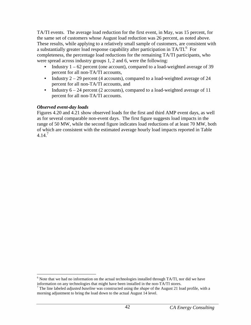
CA Energy Consulting 42
TA/TI events. The average load reduction for the first event, in May, was 15 percent, for the same set of customers whose August load reduction was 26 percent, as noted above. These results, while applying to a relatively small sample of customers, are consistent with a substantially greater load response capability after participation in TA/TI.6 For completeness, the percentage load reductions for the remaining TA/TI participants, who were spread across industry groups 1, 2 and 6, were the following:
• Industry 1 – 62 percent (one account), compared to a load-weighted average of 39 percent for all non-TA/TI accounts,
• Industry 2 – 29 percent (4 accounts), compared to a load-weighted average of 24 percent for all non-TA/TI accounts, and
• Industry 6 – 24 percent (2 accounts), compared to a load-weighted average of 11 percent for all non-TA/TI accounts.
Observed event-day loads Figures 4.20 and 4.21 show observed loads for the first and third AMP event days, as well as for several comparable non-event days. The first figure suggests load impacts in the range of 50 MW, while the second figure indicates load reductions of at least 70 MW, both of which are consistent with the estimated average hourly load impacts reported in Table 4.14.7
6 Note that we had no information on the actual technologies installed through TA/TI, nor did we have information on any technologies that might have been installed in the non-TA/TI stores. 7 The line labeled adjusted baseline was constructed using the shape of the August 21 load profile, with a morning adjustment to bring the load down to the actual August 14 level.
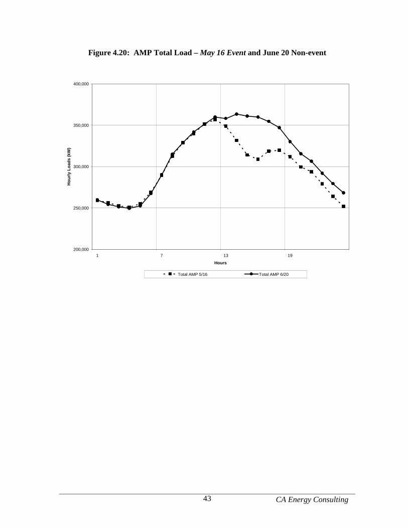
CA Energy Consulting 43
Figure 4.20: AMP Total Load – May 16 Event and June 20 Non-event
200,000
250,000
300,000
350,000
400,000
1 7 13 19
Hours
Hou
rly L
oads
(kW
)
Total AMP 5/16 Total AMP 6/20
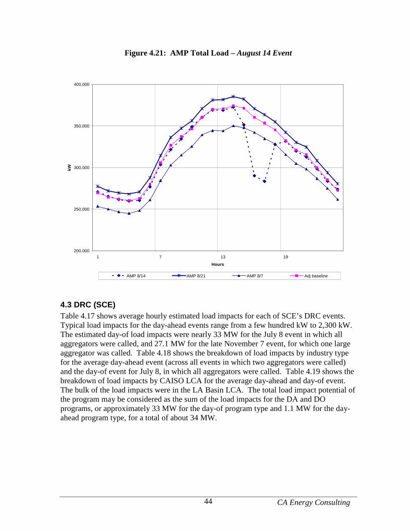
CA Energy Consulting 44
Figure 4.21: AMP Total Load – August 14 Event
200,000
250,000
300,000
350,000
400,000
1 7 13 19
Hours
kW
AMP 8/14 AMP 8/21 AMP 8/7 Adj baseline
4.3 DRC (SCE) Table 4.17 shows average hourly estimated load impacts for each of SCE’s DRC events. Typical load impacts for the day-ahead events range from a few hundred kW to 2,300 kW. The estimated day-of load impacts were nearly 33 MW for the July 8 event in which all aggregators were called, and 27.1 MW for the late November 7 event, for which one large aggregator was called. Table 4.18 shows the breakdown of load impacts by industry type for the average day-ahead event (across all events in which two aggregators were called) and the day-of event for July 8, in which all aggregators were called. Table 4.19 shows the breakdown of load impacts by CAISO LCA for the average day-ahead and day-of event. The bulk of the load impacts were in the LA Basin LCA. The total load impact potential of the program may be considered as the sum of the load impacts for the DA and DO programs, or approximately 33 MW for the day-of program type and 1.1 MW for the day-ahead program type, for a total of about 34 MW.
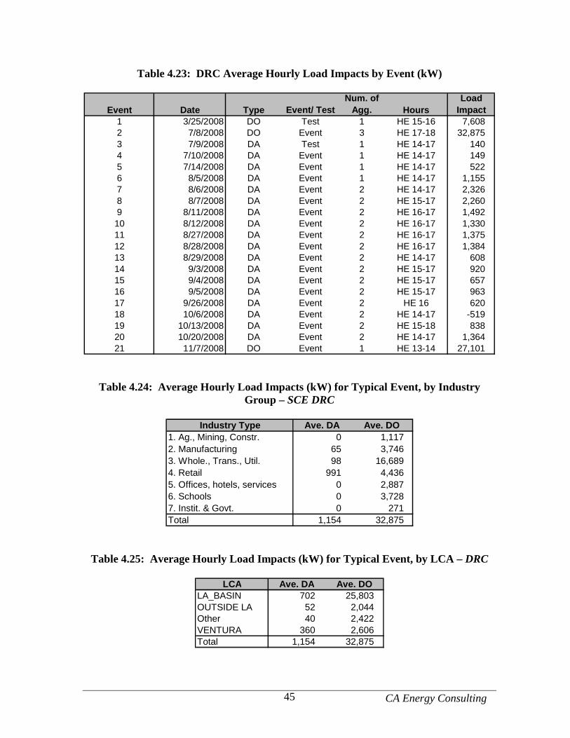
CA Energy Consulting 45
Table 4.23: DRC Average Hourly Load Impacts by Event (kW)
Event Date Type Event/ TestNum. of
Agg. HoursLoad
Impact1 3/25/2008 DO Test 1 HE 15-16 7,6082 7/8/2008 DO Event 3 HE 17-18 32,8753 7/9/2008 DA Test 1 HE 14-17 1404 7/10/2008 DA Event 1 HE 14-17 1495 7/14/2008 DA Event 1 HE 14-17 5226 8/5/2008 DA Event 1 HE 14-17 1,1557 8/6/2008 DA Event 2 HE 14-17 2,3268 8/7/2008 DA Event 2 HE 15-17 2,2609 8/11/2008 DA Event 2 HE 16-17 1,49210 8/12/2008 DA Event 2 HE 16-17 1,33011 8/27/2008 DA Event 2 HE 16-17 1,37512 8/28/2008 DA Event 2 HE 16-17 1,38413 8/29/2008 DA Event 2 HE 14-17 60814 9/3/2008 DA Event 2 HE 15-17 92015 9/4/2008 DA Event 2 HE 15-17 65716 9/5/2008 DA Event 2 HE 15-17 96317 9/26/2008 DA Event 2 HE 16 62018 10/6/2008 DA Event 2 HE 14-17 -51919 10/13/2008 DA Event 2 HE 15-18 83820 10/20/2008 DA Event 2 HE 14-17 1,36421 11/7/2008 DO Event 1 HE 13-14 27,101
Table 4.24: Average Hourly Load Impacts (kW) for Typical Event, by Industry Group – SCE DRC
Industry Type Ave. DA Ave. DO
1. Ag., Mining, Constr. 0 1,1172. Manufacturing 65 3,7463. Whole., Trans., Util. 98 16,6894. Retail 991 4,4365. Offices, hotels, services 0 2,8876. Schools 0 3,7287. Instit. & Govt. 0 271Total 1,154 32,875
Table 4.25: Average Hourly Load Impacts (kW) for Typical Event, by LCA – DRC
LCA Ave. DA Ave. DOLA_BASIN 702 25,803OUTSIDE LA 52 2,044Other 40 2,422VENTURA 360 2,606Total 1,154 32,875
CA Energy Consulting 46
Hourly load impacts Tables 4.20a and 4.20b show aggregate and per customer (respectively) hourly reference load, observed load, and load impact values for the average SCE DRC event, where the average event is defined as the sum of the averages of the typical DA events for which both aggregators were called (events 7 through 20), and the second DO event (July 8), for which all three aggregators were called (since both types of events may be called on the same day). Hourly load impacts were about 21 percent of the reference load in hours 17-18 which were the hours of the DO event. The 10th and 90th percentile load impacts in those hours are estimated to lie about 7 percent below and above the estimated load impacts for the average event. Figure 4.22 illustrates the loads and load impacts for the average event, while Figure 4.23 illustrates the uncertainty-adjusted load impacts. The bulk of the DRC load impacts come from the DO contracts. This is shown in the summary of average hourly load impacts in Table 4.17 above, and illustrated in Figure 4.24 below, which shows loads and load impacts for a typical DA event (August 27), for which the average load impact was 1.4 MW.
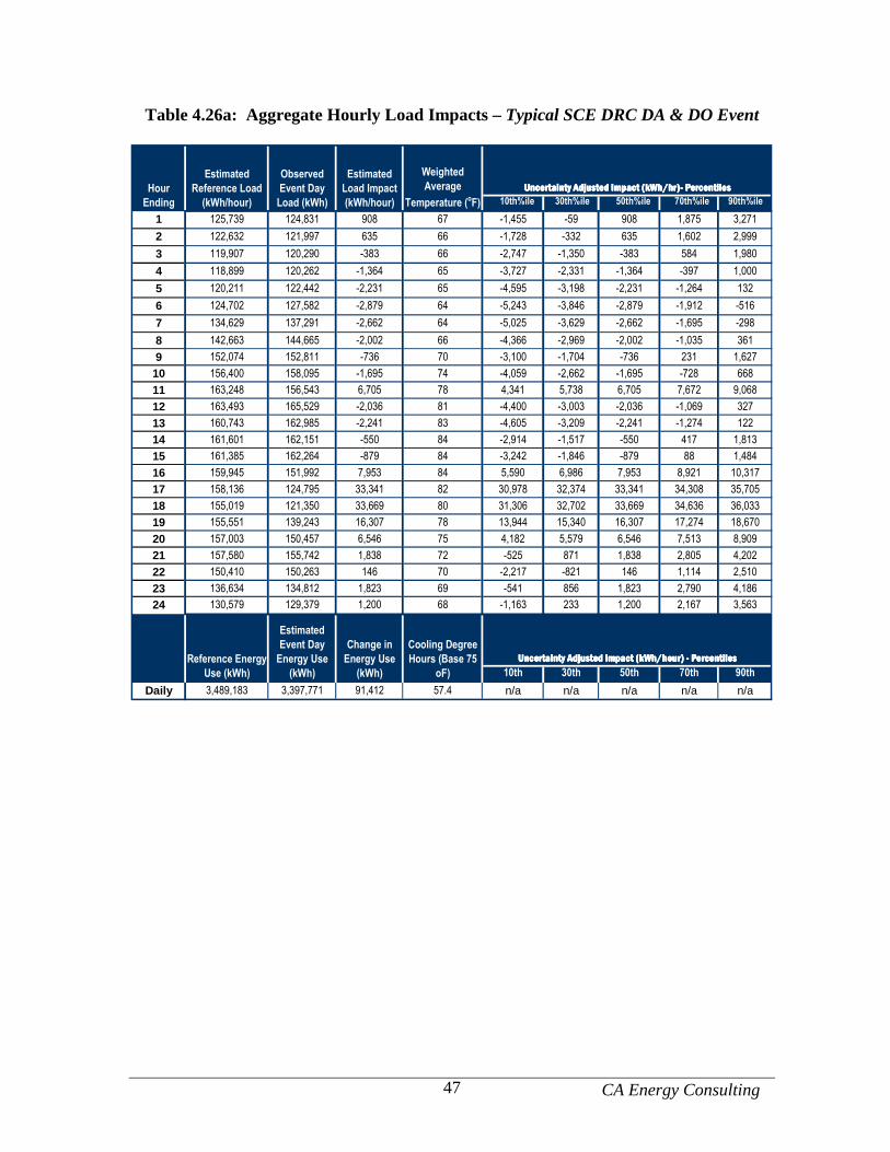
CA Energy Consulting 47
Table 4.26a: Aggregate Hourly Load Impacts – Typical SCE DRC DA & DO Event
Uncertainty Adjusted Impact (kWh/hr)- PercentilesUncertainty Adjusted Impact (kWh/hr)- PercentilesUncertainty Adjusted Impact (kWh/hr)- PercentilesUncertainty Adjusted Impact (kWh/hr)- Percentiles
10th%ile 30th%ile 50th%ile 70th%ile 90th%ile
1 125,739 124,831 908 67 -1,455 -59 908 1,875 3,271
2 122,632 121,997 635 66 -1,728 -332 635 1,602 2,999
3 119,907 120,290 -383 66 -2,747 -1,350 -383 584 1,980
4 118,899 120,262 -1,364 65 -3,727 -2,331 -1,364 -397 1,000
5 120,211 122,442 -2,231 65 -4,595 -3,198 -2,231 -1,264 132
6 124,702 127,582 -2,879 64 -5,243 -3,846 -2,879 -1,912 -516
7 134,629 137,291 -2,662 64 -5,025 -3,629 -2,662 -1,695 -298
8 142,663 144,665 -2,002 66 -4,366 -2,969 -2,002 -1,035 361
9 152,074 152,811 -736 70 -3,100 -1,704 -736 231 1,627
10 156,400 158,095 -1,695 74 -4,059 -2,662 -1,695 -728 668
11 163,248 156,543 6,705 78 4,341 5,738 6,705 7,672 9,068
12 163,493 165,529 -2,036 81 -4,400 -3,003 -2,036 -1,069 327
13 160,743 162,985 -2,241 83 -4,605 -3,209 -2,241 -1,274 122
14 161,601 162,151 -550 84 -2,914 -1,517 -550 417 1,813
15 161,385 162,264 -879 84 -3,242 -1,846 -879 88 1,484
16 159,945 151,992 7,953 84 5,590 6,986 7,953 8,921 10,317
17 158,136 124,795 33,341 82 30,978 32,374 33,341 34,308 35,705
18 155,019 121,350 33,669 80 31,306 32,702 33,669 34,636 36,033
19 155,551 139,243 16,307 78 13,944 15,340 16,307 17,274 18,670
20 157,003 150,457 6,546 75 4,182 5,579 6,546 7,513 8,909
21 157,580 155,742 1,838 72 -525 871 1,838 2,805 4,202
22 150,410 150,263 146 70 -2,217 -821 146 1,114 2,510
23 136,634 134,812 1,823 69 -541 856 1,823 2,790 4,186
24 130,579 129,379 1,200 68 -1,163 233 1,200 2,167 3,563
Uncertainty Adjusted Impact (kWh/hour) - PercentilesUncertainty Adjusted Impact (kWh/hour) - PercentilesUncertainty Adjusted Impact (kWh/hour) - PercentilesUncertainty Adjusted Impact (kWh/hour) - Percentiles
10th 30th 50th 70th 90th
Daily 3,489,183 3,397,771 91,412 57.4 n/a n/a n/a n/a n/a
Weighted
Average
Temperature (oF)
Reference Energy
Use (kWh)
Estimated
Event Day
Energy Use
(kWh)
Change in
Energy Use
(kWh)
Cooling Degree
Hours (Base 75
oF)
Hour
Ending
Estimated
Reference Load
(kWh/hour)
Observed
Event Day
Load (kWh)
Estimated
Load Impact
(kWh/hour)
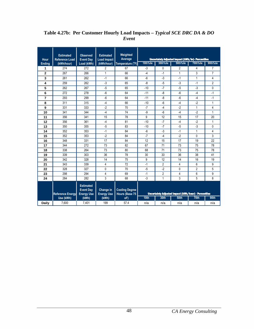
CA Energy Consulting 48
Table 4.27b: Per Customer Hourly Load Impacts – Typical SCE DRC DA & DO Event
Uncertainty Adjusted Impact (kWh/hr)- PercentilesUncertainty Adjusted Impact (kWh/hr)- PercentilesUncertainty Adjusted Impact (kWh/hr)- PercentilesUncertainty Adjusted Impact (kWh/hr)- Percentiles
10th%ile 30th%ile 50th%ile 70th%ile 90th%ile
1 274 272 2 67 -3 0 2 4 7
2 267 266 1 66 -4 -1 1 3 7
3 261 262 -1 66 -6 -3 -1 1 4
4 259 262 -3 65 -8 -5 -3 -1 2
5 262 267 -5 65 -10 -7 -5 -3 0
6 272 278 -6 64 -11 -8 -6 -4 -1
7 293 299 -6 64 -11 -8 -6 -4 -1
8 311 315 -4 66 -10 -6 -4 -2 1
9 331 333 -2 70 -7 -4 -2 1 4
10 341 344 -4 74 -9 -6 -4 -2 1
11 356 341 15 78 9 12 15 17 20
12 356 361 -4 81 -10 -7 -4 -2 1
13 350 355 -5 83 -10 -7 -5 -3 0
14 352 353 -1 84 -6 -3 -1 1 4
15 352 353 -2 84 -7 -4 -2 0 3
16 348 331 17 84 12 15 17 19 22
17 344 272 73 82 67 71 73 75 78
18 338 264 73 80 68 71 73 75 78
19 339 303 36 78 30 33 36 38 41
20 342 328 14 75 9 12 14 16 19
21 343 339 4 72 -1 2 4 6 9
22 328 327 0 70 -5 -2 0 2 5
23 298 294 4 69 -1 2 4 6 9
24 284 282 3 68 -3 1 3 5 8
Uncertainty Adjusted Impact (kWh/hour) - PercentilesUncertainty Adjusted Impact (kWh/hour) - PercentilesUncertainty Adjusted Impact (kWh/hour) - PercentilesUncertainty Adjusted Impact (kWh/hour) - Percentiles
10th 30th 50th 70th 90th
Daily 7,600 7,401 199 57.4 n/a n/a n/a n/a n/a
Hour
Ending
Estimated
Reference Load
(kWh/hour)
Observed
Event Day
Load (kWh)
Estimated
Load Impact
(kWh/hour)
Weighted
Average
Temperature (oF)
Reference Energy
Use (kWh)
Estimated
Event Day
Energy Use
(kWh)
Change in
Energy Use
(kWh)
Cooling Degree
Hours (Base 75
oF)
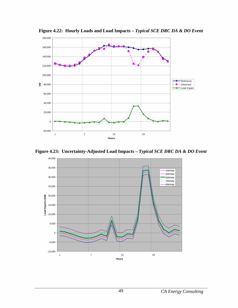
CA Energy Consulting 49
Figure 4.22: Hourly Loads and Load Impacts – Typical SCE DRC DA & DO Event
-20,000
0
20,000
40,000
60,000
80,000
100,000
120,000
140,000
160,000
180,000
1 7 13 19
Hours
kW
Reference
Observed
Load impact
Figure 4.23: Uncertainty-Adjusted Load Impacts – Typical SCE DRC DA & DO Event
-10,000
-5,000
0
5,000
10,000
15,000
20,000
25,000
30,000
35,000
40,000
1 7 13 19
Hours
Load
Impa
cts
(kW
)
10th%ile
30th%ile
50th%ile
70th%ile
90th%ile
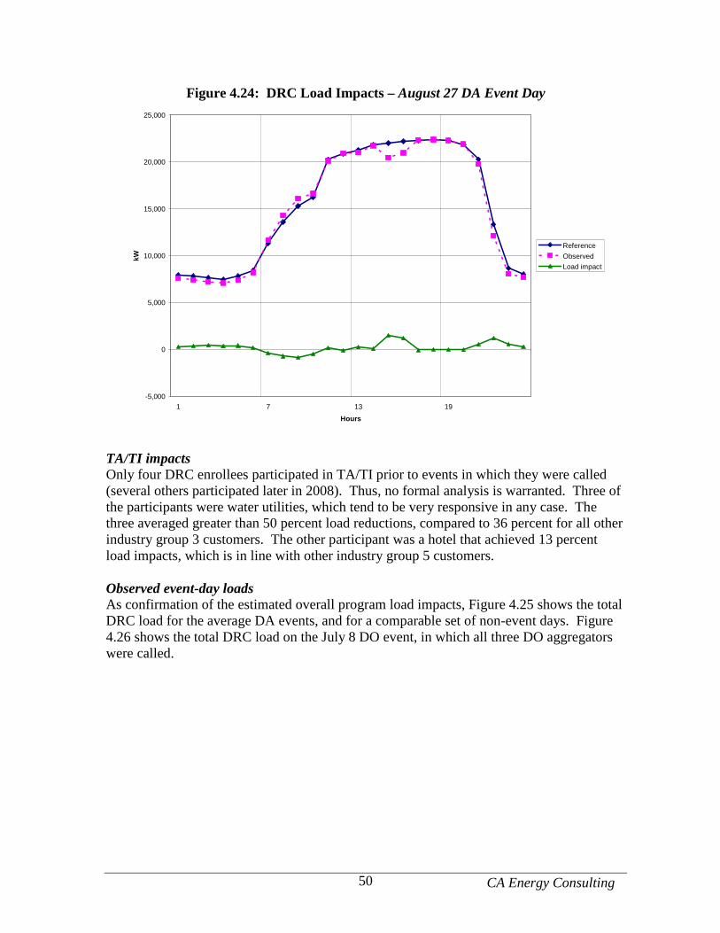
CA Energy Consulting 50
Figure 4.24: DRC Load Impacts – August 27 DA Event Day
-5,000
0
5,000
10,000
15,000
20,000
25,000
1 7 13 19
Hours
kW
Reference
Observed
Load impact
TA/TI impacts Only four DRC enrollees participated in TA/TI prior to events in which they were called (several others participated later in 2008). Thus, no formal analysis is warranted. Three of the participants were water utilities, which tend to be very responsive in any case. The three averaged greater than 50 percent load reductions, compared to 36 percent for all other industry group 3 customers. The other participant was a hotel that achieved 13 percent load impacts, which is in line with other industry group 5 customers. Observed event-day loads As confirmation of the estimated overall program load impacts, Figure 4.25 shows the total DRC load for the average DA events, and for a comparable set of non-event days. Figure 4.26 shows the total DRC load on the July 8 DO event, in which all three DO aggregators were called.
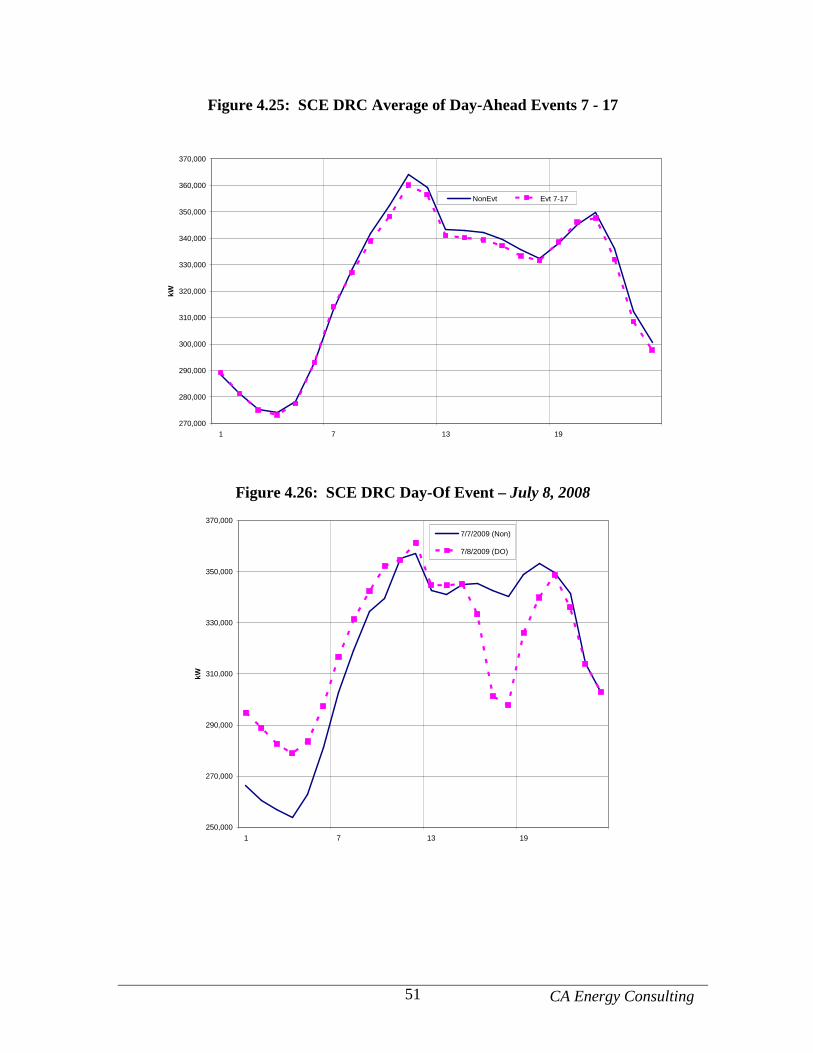
CA Energy Consulting 51
Figure 4.25: SCE DRC Average of Day-Ahead Events 7 - 17
270,000
280,000
290,000
300,000
310,000
320,000
330,000
340,000
350,000
360,000
370,000
1 7 13 19
kW
NonEvt Evt 7-17
Figure 4.26: SCE DRC Day-Of Event – July 8, 2008
250,000
270,000
290,000
310,000
330,000
350,000
370,000
1 7 13 19
kW
7/7/2009 (Non)
7/8/2009 (DO)
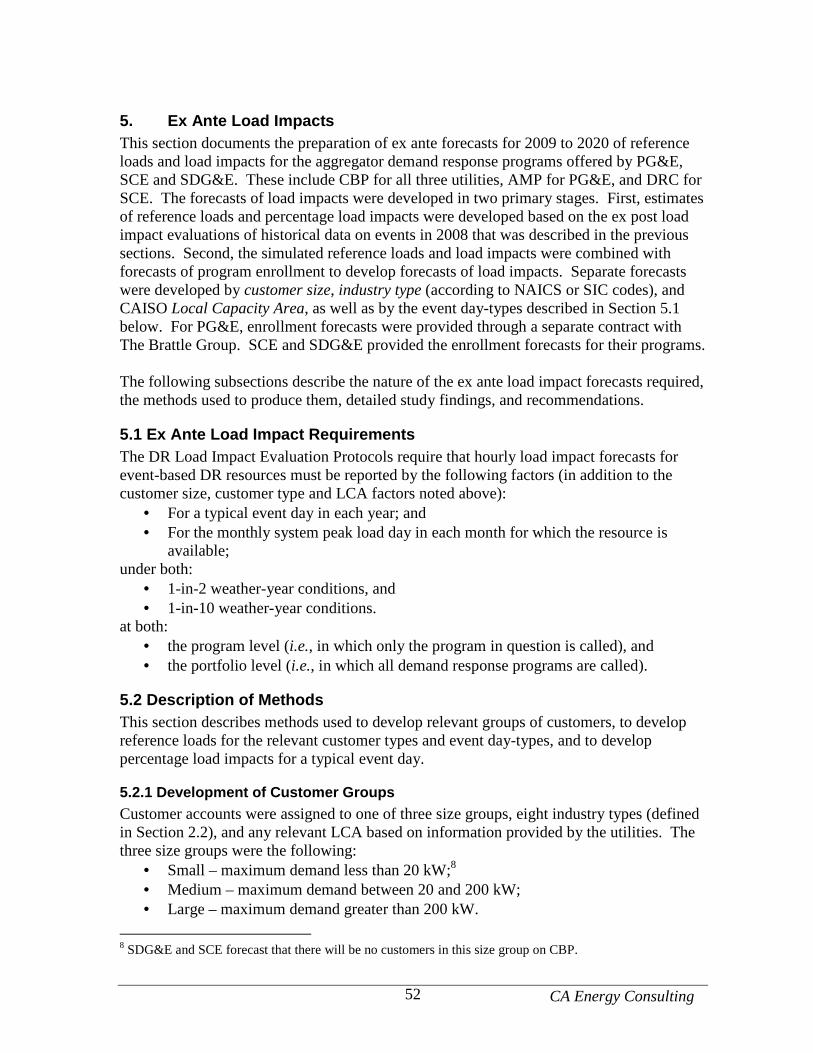
CA Energy Consulting 52
5. Ex Ante Load Impacts This section documents the preparation of ex ante forecasts for 2009 to 2020 of reference loads and load impacts for the aggregator demand response programs offered by PG&E, SCE and SDG&E. These include CBP for all three utilities, AMP for PG&E, and DRC for SCE. The forecasts of load impacts were developed in two primary stages. First, estimates of reference loads and percentage load impacts were developed based on the ex post load impact evaluations of historical data on events in 2008 that was described in the previous sections. Second, the simulated reference loads and load impacts were combined with forecasts of program enrollment to develop forecasts of load impacts. Separate forecasts were developed by customer size, industry type (according to NAICS or SIC codes), and CAISO Local Capacity Area, as well as by the event day-types described in Section 5.1 below. For PG&E, enrollment forecasts were provided through a separate contract with The Brattle Group. SCE and SDG&E provided the enrollment forecasts for their programs. The following subsections describe the nature of the ex ante load impact forecasts required, the methods used to produce them, detailed study findings, and recommendations.
5.1 Ex Ante Load Impact Requirements The DR Load Impact Evaluation Protocols require that hourly load impact forecasts for event-based DR resources must be reported by the following factors (in addition to the customer size, customer type and LCA factors noted above):
• For a typical event day in each year; and • For the monthly system peak load day in each month for which the resource is
available; under both:
• 1-in-2 weather-year conditions, and • 1-in-10 weather-year conditions.
at both: • the program level (i.e., in which only the program in question is called), and • the portfolio level (i.e., in which all demand response programs are called).
5.2 Description of Methods This section describes methods used to develop relevant groups of customers, to develop reference loads for the relevant customer types and event day-types, and to develop percentage load impacts for a typical event day.
5.2.1 Development of Customer Groups Customer accounts were assigned to one of three size groups, eight industry types (defined in Section 2.2), and any relevant LCA based on information provided by the utilities. The three size groups were the following:
• Small – maximum demand less than 20 kW;8 • Medium – maximum demand between 20 and 200 kW; • Large – maximum demand greater than 200 kW.
8 SDG&E and SCE forecast that there will be no customers in this size group on CBP.
CA Energy Consulting 53
The specific definition of “maximum demand” differed by utility. For PG&E and SCE, the size definition was based on the tariff on which the customer is served. For example, a tariff may require that a customer’s monthly peak demand exceeds 20kW for three out of the previous twelve months. For SDG&E, the size definition was based on each customer’s maximum summer on-peak demand. PG&E and SCE provided the ability to associate customers with an LCA. PG&E mapped each distribution feeder to one of its seven LCAs, while SCE based its mapping on a combination of substations and zip codes.
5.2.2 Development of Reference Loads and Load Impac ts Reference loads and load impacts for all of the above factors were developed in the following series of steps:
1. Define data sources 2. Simulate reference loads by cell 3. Calculate forecast percentage load impacts by cell 4. Apply percentage load impacts to the reference loads 5. Scale the reference loads using enrollment forecasts
Each of these steps is described below. Define data sources No major design changes are planned for any of the aggregator programs. Because of this, there is a close link between the results of the ex post analyses conducted for the 2008 program year and the ex ante load impacts. That is, the historical customer loads serve as the source of the ex ante reference loads and the historical percentage load impacts serve as the source of the ex ante load impacts. There is no need to convert historical load impacts to price elasticities because the price signal is not expected to change. This contrasts with our CPP/PDP ex ante load impact study, in which elasticity estimates were developed to account for significant changes in event day prices in the forecast period. Simulate reference loads For each program, we estimated regression equations for each customer account, using data for 2008. The purpose of these equations was to simulate reference loads by customer type for the various scenarios required by the Protocols (e.g., the typical event day in a 1-in-2 weather year). These equations were similar in design to the ex post load impact equations described in Section 3.1. There was one primary difference between the ex post and ex ante regression models: the ex ante models excluded the morning-usage variable. While this variable is useful for increasing accuracy in estimating ex post load impacts for particular events, it complicates the use of the equations in ex ante simulation. That is, it requires one to separately simulate the level of the morning load.
CA Energy Consulting 54
The definitions of the 1-in-2 and 1-in-10 weather years differed by utility, as shown in Table 5.1. For SDG&E, the year shown was used to generate the typical event days. Unlike SCE and PG&E, SDG&E selected from different years to develop its scenarios of peak load days by month.
Table 5.1: Weather Year Definitions by Utility
Utility 1-in-2 Weather Year 1-in-10 Weather Year PG&E 2004 2003 SCE 2002 1998
SDG&E 2004* 2007* For SCE’s CBP and DRC programs, we developed separate load profiles at three levels of aggregation for each size category: all enrolled customers; by industry group; and by LCA. These correspond to the reporting levels required in the Protocols. This method is feasible because SCE did not provide enrollments by cell (i.e., combinations of industry groups and LCAs) for these programs. Specifically, SCE specified that CBP enrollments would increase 5 percent per year through 2012; and SCE forecast DRC enrollments by aggregator and notice level (day ahead and day of). For PG&E’s AMP and CBP programs, we developed per-customer load profiles for all interactions of size group, industry group, and LCA. Because of small sample sizes in some cells, we pooled all of the customer load profiles across LCAs to arrive at a set of simulation coefficients that was common to each size and industry group combination. Differences in the load profiles across LCAs were solely due to differences in the weather conditions used in the simulations. This method conformed to the enrollment forecast developed for PG&E by The Brattle Group, which forecast the number of enrolled customers in each cell. For SDG&E’s CBP program, we developed per-customer load profiles for by industry group, notice level and hours of availability (e.g., manufacturing customers called with day-ahead notice for a four-hour event window). This method conformed to the enrollment forecast provided by SDG&E, which specified the number of enrolled customers within each group. Calculate forecast percentage load impacts The first step in developing the forecast percentage load impacts was to determine the definition of a “typical event day” during which the load impacts were to be measured. This was complicated by the fact that the aggregator DR program events, as implemented in 2008, differ somewhat from those of some of the other DR programs, in that many of the events called differed in terms of program type (e.g., day-ahead or day-of), event length (e.g., as short as one hour, to as long as 6 hours, depending in part on the aggregator contracts), and the particular hours called. As a result, in many cases there was no obvious definition of a “typical” event in 2008. However, a definition of a typical event was needed for the ex ante forecast period that would allow us to forecast the load impact that would occur if all nominated customers were called on the same day. The following
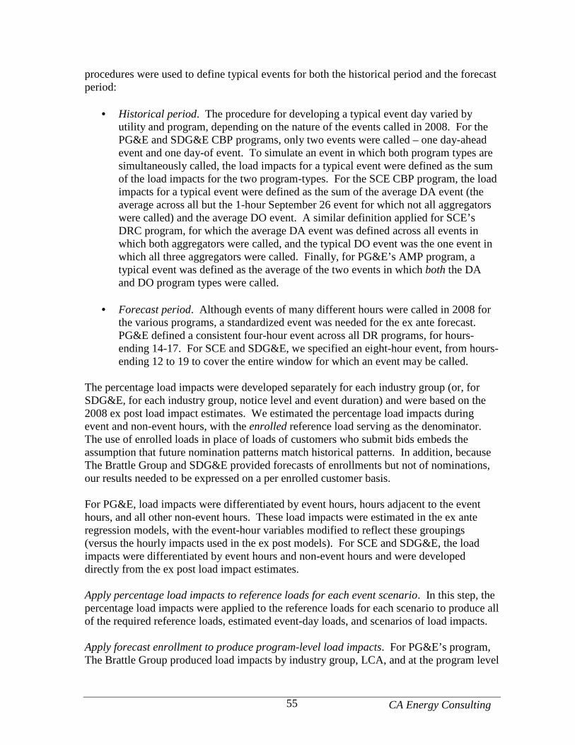
CA Energy Consulting 55
procedures were used to define typical events for both the historical period and the forecast period:
• Historical period. The procedure for developing a typical event day varied by utility and program, depending on the nature of the events called in 2008. For the PG&E and SDG&E CBP programs, only two events were called – one day-ahead event and one day-of event. To simulate an event in which both program types are simultaneously called, the load impacts for a typical event were defined as the sum of the load impacts for the two program-types. For the SCE CBP program, the load impacts for a typical event were defined as the sum of the average DA event (the average across all but the 1-hour September 26 event for which not all aggregators were called) and the average DO event. A similar definition applied for SCE’s DRC program, for which the average DA event was defined across all events in which both aggregators were called, and the typical DO event was the one event in which all three aggregators were called. Finally, for PG&E’s AMP program, a typical event was defined as the average of the two events in which both the DA and DO program types were called.
• Forecast period. Although events of many different hours were called in 2008 for the various programs, a standardized event was needed for the ex ante forecast. PG&E defined a consistent four-hour event across all DR programs, for hours-ending 14-17. For SCE and SDG&E, we specified an eight-hour event, from hours-ending 12 to 19 to cover the entire window for which an event may be called.
The percentage load impacts were developed separately for each industry group (or, for SDG&E, for each industry group, notice level and event duration) and were based on the 2008 ex post load impact estimates. We estimated the percentage load impacts during event and non-event hours, with the enrolled reference load serving as the denominator. The use of enrolled loads in place of loads of customers who submit bids embeds the assumption that future nomination patterns match historical patterns. In addition, because The Brattle Group and SDG&E provided forecasts of enrollments but not of nominations, our results needed to be expressed on a per enrolled customer basis. For PG&E, load impacts were differentiated by event hours, hours adjacent to the event hours, and all other non-event hours. These load impacts were estimated in the ex ante regression models, with the event-hour variables modified to reflect these groupings (versus the hourly impacts used in the ex post models). For SCE and SDG&E, the load impacts were differentiated by event hours and non-event hours and were developed directly from the ex post load impact estimates. Apply percentage load impacts to reference loads for each event scenario. In this step, the percentage load impacts were applied to the reference loads for each scenario to produce all of the required reference loads, estimated event-day loads, and scenarios of load impacts. Apply forecast enrollment to produce program-level load impacts. For PG&E’s program, The Brattle Group produced load impacts by industry group, LCA, and at the program level
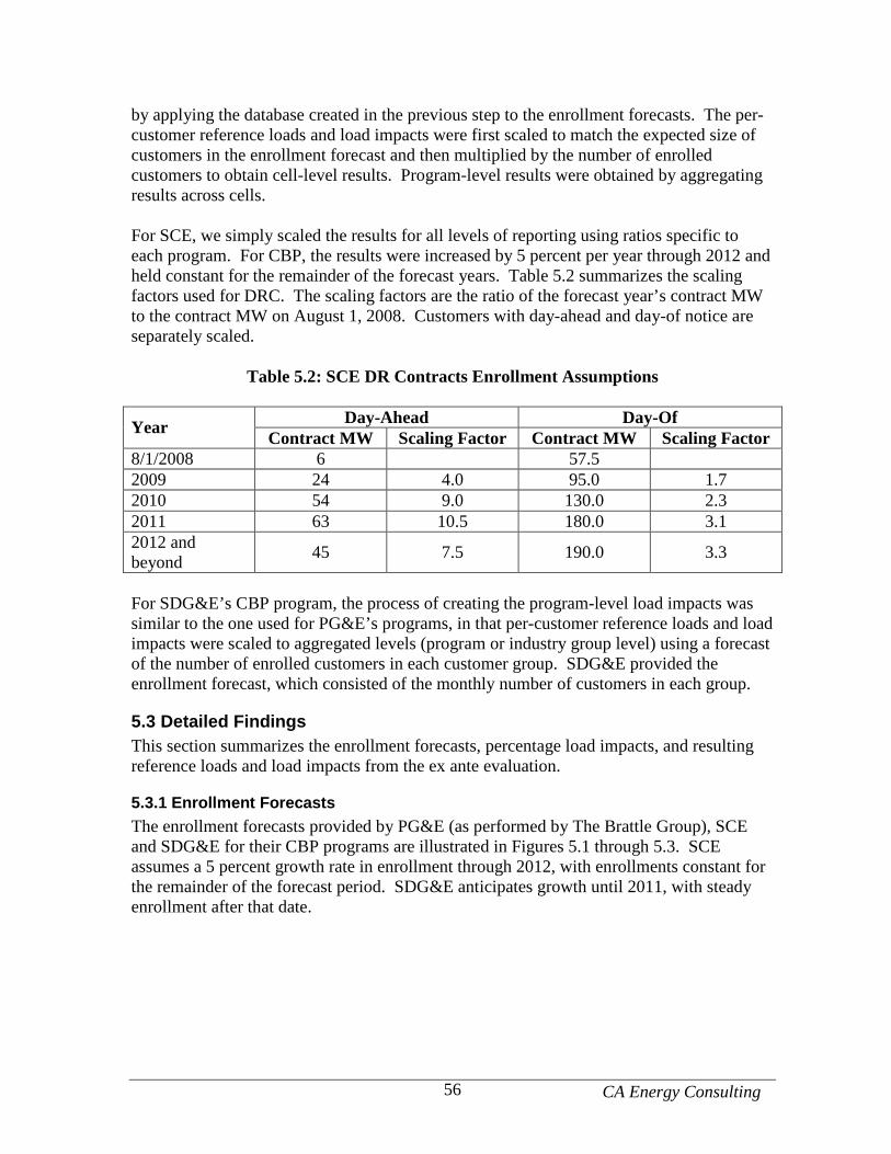
CA Energy Consulting 56
by applying the database created in the previous step to the enrollment forecasts. The per-customer reference loads and load impacts were first scaled to match the expected size of customers in the enrollment forecast and then multiplied by the number of enrolled customers to obtain cell-level results. Program-level results were obtained by aggregating results across cells. For SCE, we simply scaled the results for all levels of reporting using ratios specific to each program. For CBP, the results were increased by 5 percent per year through 2012 and held constant for the remainder of the forecast years. Table 5.2 summarizes the scaling factors used for DRC. The scaling factors are the ratio of the forecast year’s contract MW to the contract MW on August 1, 2008. Customers with day-ahead and day-of notice are separately scaled.
Table 5.2: SCE DR Contracts Enrollment Assumptions
Day-Ahead Day-Of Year Contract MW Scaling Factor Contract MW Scaling Factor
8/1/2008 6 57.5 2009 24 4.0 95.0 1.7 2010 54 9.0 130.0 2.3 2011 63 10.5 180.0 3.1 2012 and beyond
45 7.5 190.0 3.3
For SDG&E’s CBP program, the process of creating the program-level load impacts was similar to the one used for PG&E’s programs, in that per-customer reference loads and load impacts were scaled to aggregated levels (program or industry group level) using a forecast of the number of enrolled customers in each customer group. SDG&E provided the enrollment forecast, which consisted of the monthly number of customers in each group.
5.3 Detailed Findings This section summarizes the enrollment forecasts, percentage load impacts, and resulting reference loads and load impacts from the ex ante evaluation.
5.3.1 Enrollment Forecasts The enrollment forecasts provided by PG&E (as performed by The Brattle Group), SCE and SDG&E for their CBP programs are illustrated in Figures 5.1 through 5.3. SCE assumes a 5 percent growth rate in enrollment through 2012, with enrollments constant for the remainder of the forecast period. SDG&E anticipates growth until 2011, with steady enrollment after that date.
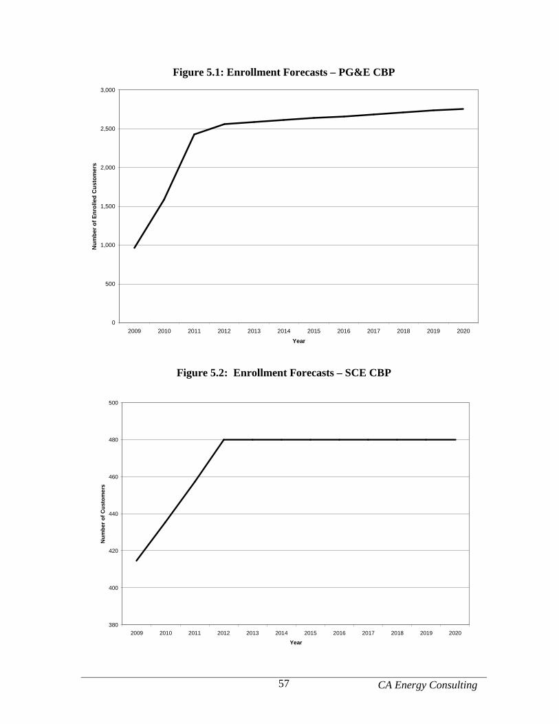
CA Energy Consulting 57
Figure 5.1: Enrollment Forecasts – PG&E CBP
0
500
1,000
1,500
2,000
2,500
3,000
2009 2010 2011 2012 2013 2014 2015 2016 2017 2018 2019 2020
Year
Num
ber
of E
nrol
led
Cus
tom
ers
Figure 5.2: Enrollment Forecasts – SCE CBP
380
400
420
440
460
480
500
2009 2010 2011 2012 2013 2014 2015 2016 2017 2018 2019 2020
Year
Num
ber
of C
usto
mer
s
CA Energy Consulting 58
Figure 5.3: Enrollment Forecasts – SDG&E CBP
0
100
200
300
Oct 08enrolled
Oct-09 Oct-10 Oct-11 Oct-12 Oct-13 Oct-14 Oct-15 Oct-16 Oct-17 Oct-18 Oct-19
Month/Year
Cus
tom
er A
ccou
nts
0
10
20
30
40
50
60
Enr
olle
d Lo
ad (
MW
)
DA
DO
MW
Figure 5.4 summarizes SCE’s DRC contract load amounts by DA and DO program types for 2008 and the expected contract amounts through 2012. We scaled the DRC reference loads to correspond to the expected growth in contract amounts over that period. Figure 5.5 summarizes PG&E’s AMP enrollment forecast. Enrollments are expected to increase from 749 customers in May 2009 to 2,311 by May 2011, at which point the number of enrolled customers remains constant through 2020.
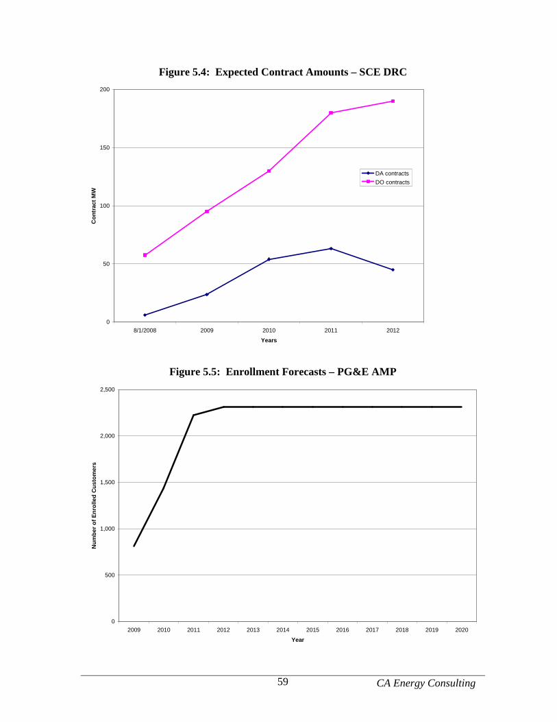
CA Energy Consulting 59
Figure 5.4: Expected Contract Amounts – SCE DRC
0
50
100
150
200
8/1/2008 2009 2010 2011 2012
Years
Con
trac
t MW
DA contracts
DO contracts
Figure 5.5: Enrollment Forecasts – PG&E AMP
0
500
1,000
1,500
2,000
2,500
2009 2010 2011 2012 2013 2014 2015 2016 2017 2018 2019 2020
Year
Num
ber
of E
nrol
led
Cus
tom
ers

CA Energy Consulting 60
5.3.2 Reference Loads and Load Impacts For each utility and program, we provide the following summary information:
1. A figure showing the hourly reference load, event-day load, and load impacts for the typical event day in a 1-in-2 weather year;
2. A pie chart showing the share of load impacts by LCA (except for SDG&E); 3. A pie chart showing the share of load impacts by industry group; 4. Average event-hour load impacts by year; and 5. Average event-hour load impacts by peak month day.
Together, these figures provide a good indication of the variability in the forecast load impacts according to the variations produced according to the Protocol’s requirements. The tables required by the Protocols are provided in the Appendix. PG&E CBP Figure PG&E CBP 1 shows the August 2012 forecast load impacts for a typical event day in a 1-in-2 weather year.9 Event-hour load impacts range from 41.6 MW to 44.4 MW, which represent approximately 7.7 percent of the enrolled reference load. Figures PG&E CBP 2 and 3 show how the load impacts are distributed by LCA and industry group. Nearly half of the load impacts come from customers in the Greater Bay Area LCA; and Retail and Manufacturing customer types account for the largest shares of load impacts, at 48 percent and 23 percent of the total respectively. Figure PG&E CBP 4 illustrates the average hourly load impact across years for the August peak day in 1-in-2 and 1-in-10 weather years. The load impacts in this figure mirror the enrollments shown in Figure 5.1, with impacts rapidly increasing to approximately 42 MW in 2011, after which there are modest increases.
9 For this program, program-level impacts and portfolio-level impacts are the same.
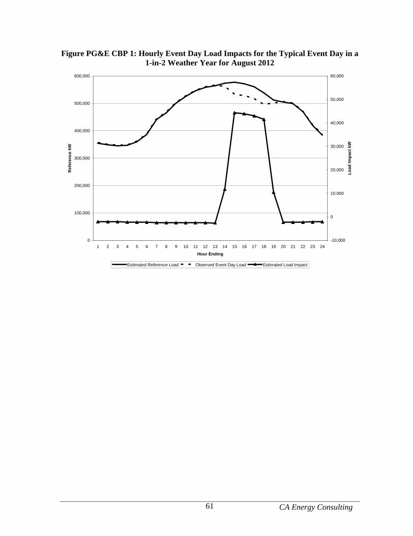
CA Energy Consulting 61
Figure PG&E CBP 1: Hourly Event Day Load Impacts for the Typical Event Day in a 1-in-2 Weather Year for August 2012
0
100,000
200,000
300,000
400,000
500,000
600,000
1 2 3 4 5 6 7 8 9 10 11 12 13 14 15 16 17 18 19 20 21 22 23 24
Hour Ending
Ref
eren
ce k
W
-10,000
0
10,000
20,000
30,000
40,000
50,000
60,000
Load
Impa
ct k
W
Estimated Reference Load Observed Event Day Load Estimated Load Impact
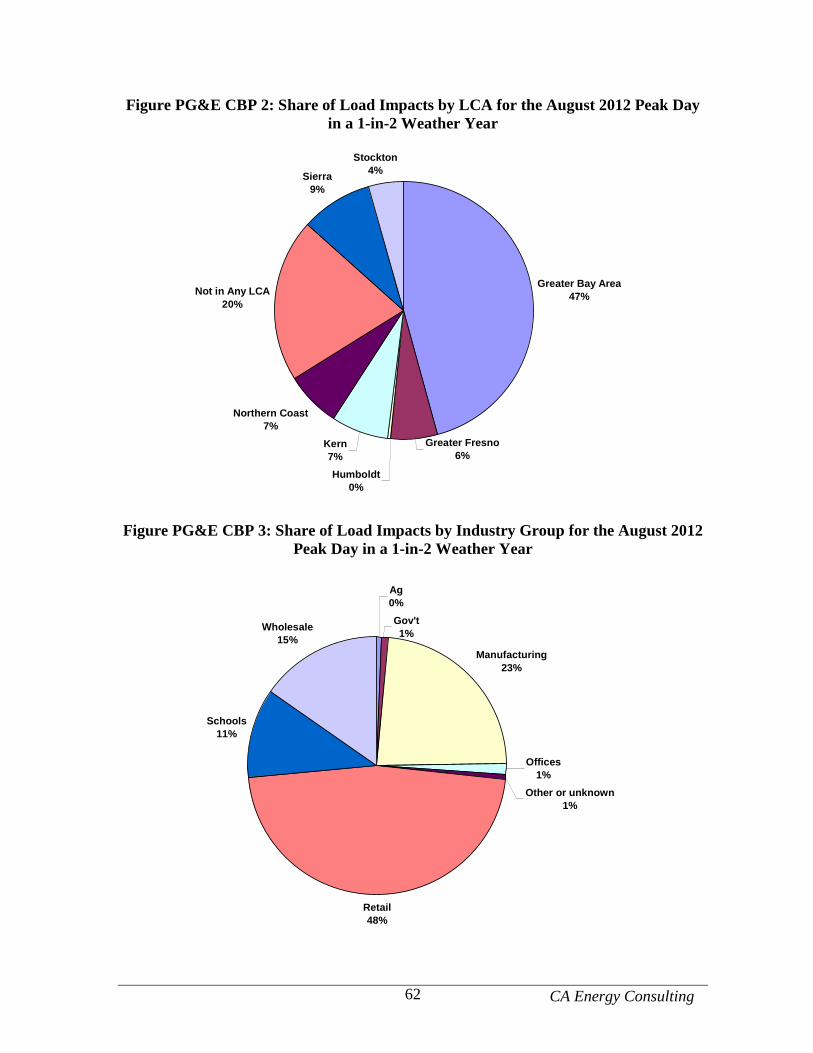
CA Energy Consulting 62
Figure PG&E CBP 2: Share of Load Impacts by LCA for the August 2012 Peak Day in a 1-in-2 Weather Year
Greater Bay Area 47%
Greater Fresno 6%
Humboldt 0%
Kern 7%
Northern Coast 7%
Not in Any LCA20%
Sierra 9%
Stockton 4%
Figure PG&E CBP 3: Share of Load Impacts by Industry Group for the August 2012
Peak Day in a 1-in-2 Weather Year
Ag0%
Gov't1%
Manufacturing23%
Offices1%
Other or unknown1%
Retail48%
Schools11%
Wholesale15%
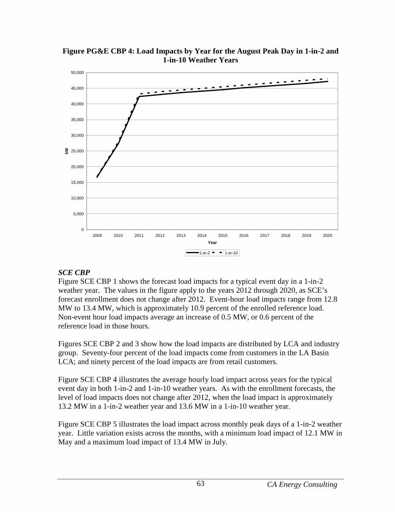
CA Energy Consulting 63
Figure PG&E CBP 4: Load Impacts by Year for the August Peak Day in 1-in-2 and 1-in-10 Weather Years
0
5,000
10,000
15,000
20,000
25,000
30,000
35,000
40,000
45,000
50,000
2009 2010 2011 2012 2013 2014 2015 2016 2017 2018 2019 2020
Year
kW
1-in-2 1-in-10
SCE CBP Figure SCE CBP 1 shows the forecast load impacts for a typical event day in a 1-in-2 weather year. The values in the figure apply to the years 2012 through 2020, as SCE’s forecast enrollment does not change after 2012. Event-hour load impacts range from 12.8 MW to 13.4 MW, which is approximately 10.9 percent of the enrolled reference load. Non-event hour load impacts average an increase of 0.5 MW, or 0.6 percent of the reference load in those hours. Figures SCE CBP 2 and 3 show how the load impacts are distributed by LCA and industry group. Seventy-four percent of the load impacts come from customers in the LA Basin LCA; and ninety percent of the load impacts are from retail customers. Figure SCE CBP 4 illustrates the average hourly load impact across years for the typical event day in both 1-in-2 and 1-in-10 weather years. As with the enrollment forecasts, the level of load impacts does not change after 2012, when the load impact is approximately 13.2 MW in a 1-in-2 weather year and 13.6 MW in a 1-in-10 weather year. Figure SCE CBP 5 illustrates the load impact across monthly peak days of a 1-in-2 weather year. Little variation exists across the months, with a minimum load impact of 12.1 MW in May and a maximum load impact of 13.4 MW in July.
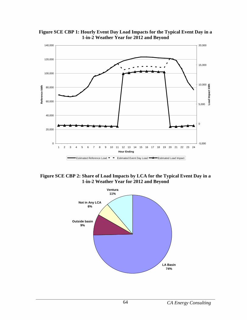
CA Energy Consulting 64
Figure SCE CBP 1: Hourly Event Day Load Impacts for the Typical Event Day in a 1-in-2 Weather Year for 2012 and Beyond
0
20,000
40,000
60,000
80,000
100,000
120,000
140,000
1 2 3 4 5 6 7 8 9 10 11 12 13 14 15 16 17 18 19 20 21 22 23 24
Hour Ending
Ref
eren
ce k
Wh
-5,000
0
5,000
10,000
15,000
20,000
Load
Impa
ct k
Wh
Estimated Reference Load Estimated Event Day Load Estimated Load Impact
Figure SCE CBP 2: Share of Load Impacts by LCA for the Typical Event Day in a 1-in-2 Weather Year for 2012 and Beyond
LA Basin74%
Outside basin9%
Not in Any LCA6%
Ventura11%
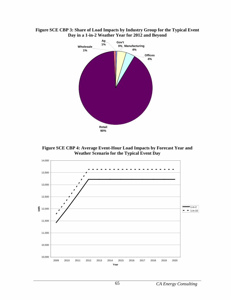
CA Energy Consulting 65
Figure SCE CBP 3: Share of Load Impacts by Industry Group for the Typical Event Day in a 1-in-2 Weather Year for 2012 and Beyond
Retail90%
Gov't0%
Ag1% Manufacturing
4%
Offices4%
Wholesale1%
Figure SCE CBP 4: Average Event-Hour Load Impacts by Forecast Year and Weather Scenario for the Typical Event Day
10,000
10,500
11,000
11,500
12,000
12,500
13,000
13,500
14,000
2009 2010 2011 2012 2013 2014 2015 2016 2017 2018 2019 2020
Year
kWh 1-in-2
1-in-10
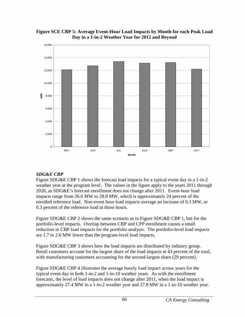
CA Energy Consulting 66
Figure SCE CBP 5: Average Event-Hour Load Impacts by Month for each Peak Load Day in a 1-in-2 Weather Year for 2012 and Beyond
0
2,000
4,000
6,000
8,000
10,000
12,000
14,000
16,000
MAY JUN JUL AUG SEP OCT
Month
kWh
SDG&E CBP Figure SDG&E CBP 1 shows the forecast load impacts for a typical event day in a 1-in-2 weather year at the program level. The values in the figure apply to the years 2011 through 2020, as SDG&E’s forecast enrollment does not change after 2011. Event-hour load impacts range from 26.6 MW to 28.8 MW, which is approximately 24 percent of the enrolled reference load. Non-event hour load impacts average an increase of 0.3 MW, or 0.3 percent of the reference load in those hours. Figure SDG&E CBP 2 shows the same scenario as in Figure SDG&E CBP 1, but for the portfolio-level impacts. Overlap between CBP and CPP enrollment causes a small reduction in CBP load impacts for the portfolio analysis. The portfolio-level load impacts are 1.7 to 2.6 MW lower than the program-level load impacts. Figure SDG&E CBP 3 shows how the load impacts are distributed by industry group. Retail customers account for the largest share of the load impacts at 43 percent of the total, with manufacturing customers accounting for the second-largest share (29 percent). Figure SDG&E CBP 4 illustrates the average hourly load impact across years for the typical event day in both 1-in-2 and 1-in-10 weather years. As with the enrollment forecasts, the level of load impacts does not change after 2011, when the load impact is approximately 27.4 MW in a 1-in-2 weather year and 27.8 MW in a 1-in-10 weather year.
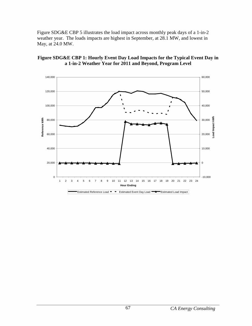
CA Energy Consulting 67
Figure SDG&E CBP 5 illustrates the load impact across monthly peak days of a 1-in-2 weather year. The loads impacts are highest in September, at 28.1 MW, and lowest in May, at 24.0 MW.
Figure SDG&E CBP 1: Hourly Event Day Load Impacts for the Typical Event Day in
a 1-in-2 Weather Year for 2011 and Beyond, Program Level
0
20,000
40,000
60,000
80,000
100,000
120,000
140,000
1 2 3 4 5 6 7 8 9 10 11 12 13 14 15 16 17 18 19 20 21 22 23 24
Hour Ending
Ref
eren
ce k
Wh
-10,000
0
10,000
20,000
30,000
40,000
50,000
60,000
Load
Impa
ct k
Wh
Estimated Reference Load Estimated Event Day Load Estimated Load Impact
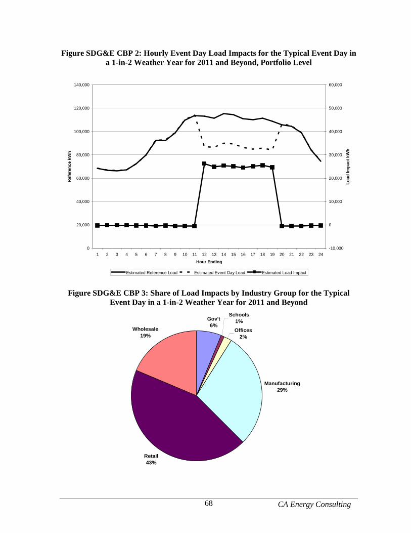
CA Energy Consulting 68
Figure SDG&E CBP 2: Hourly Event Day Load Impacts for the Typical Event Day in a 1-in-2 Weather Year for 2011 and Beyond, Portfolio Level
0
20,000
40,000
60,000
80,000
100,000
120,000
140,000
1 2 3 4 5 6 7 8 9 10 11 12 13 14 15 16 17 18 19 20 21 22 23 24
Hour Ending
Ref
eren
ce k
Wh
-10,000
0
10,000
20,000
30,000
40,000
50,000
60,000
Load
Impa
ct k
Wh
Estimated Reference Load Estimated Event Day Load Estimated Load Impact
Figure SDG&E CBP 3: Share of Load Impacts by Industry Group for the Typical
Event Day in a 1-in-2 Weather Year for 2011 and Beyond
Gov't6%
Schools1%
Offices2%
Manufacturing29%
Retail43%
Wholesale19%
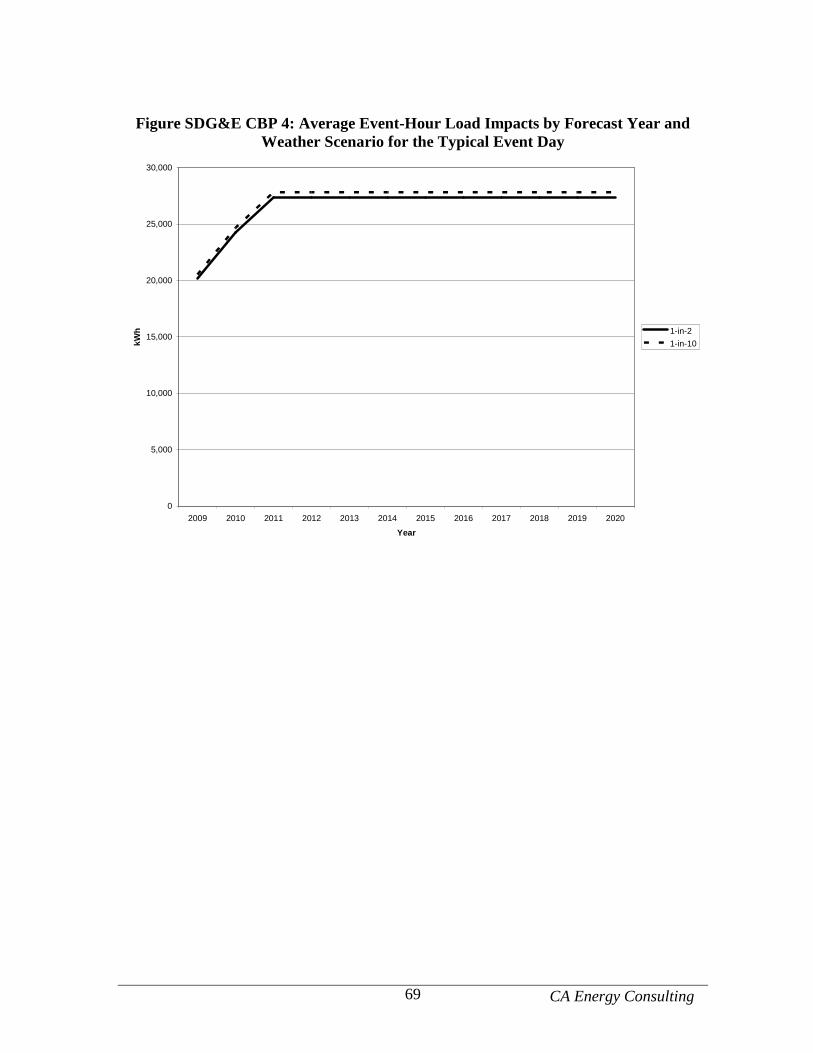
CA Energy Consulting 69
Figure SDG&E CBP 4: Average Event-Hour Load Impacts by Forecast Year and
Weather Scenario for the Typical Event Day
0
5,000
10,000
15,000
20,000
25,000
30,000
2009 2010 2011 2012 2013 2014 2015 2016 2017 2018 2019 2020
Year
kWh 1-in-2
1-in-10
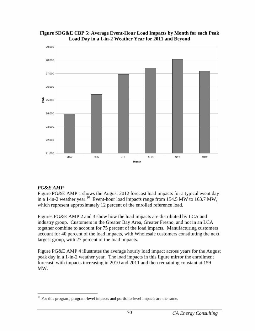
CA Energy Consulting 70
Figure SDG&E CBP 5: Average Event-Hour Load Impacts by Month for each Peak Load Day in a 1-in-2 Weather Year for 2011 and Beyond
21,000
22,000
23,000
24,000
25,000
26,000
27,000
28,000
29,000
MAY JUN JUL AUG SEP OCT
Month
kWh
PG&E AMP Figure PG&E AMP 1 shows the August 2012 forecast load impacts for a typical event day in a 1-in-2 weather year.10 Event-hour load impacts range from 154.5 MW to 163.7 MW, which represent approximately 12 percent of the enrolled reference load. Figures PG&E AMP 2 and 3 show how the load impacts are distributed by LCA and industry group. Customers in the Greater Bay Area, Greater Fresno, and not in an LCA together combine to account for 75 percent of the load impacts. Manufacturing customers account for 40 percent of the load impacts, with Wholesale customers constituting the next largest group, with 27 percent of the load impacts. Figure PG&E AMP 4 illustrates the average hourly load impact across years for the August peak day in a 1-in-2 weather year. The load impacts in this figure mirror the enrollment forecast, with impacts increasing in 2010 and 2011 and then remaining constant at 159 MW.
10 For this program, program-level impacts and portfolio-level impacts are the same.
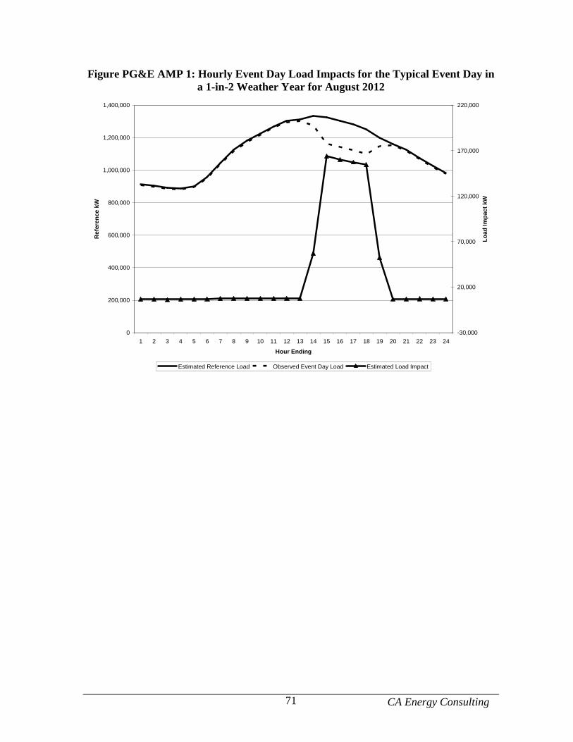
CA Energy Consulting 71
Figure PG&E AMP 1: Hourly Event Day Load Impacts for the Typical Event Day in a 1-in-2 Weather Year for August 2012
0
200,000
400,000
600,000
800,000
1,000,000
1,200,000
1,400,000
1 2 3 4 5 6 7 8 9 10 11 12 13 14 15 16 17 18 19 20 21 22 23 24
Hour Ending
Ref
eren
ce k
W
-30,000
20,000
70,000
120,000
170,000
220,000
Load
Impa
ct k
W
Estimated Reference Load Observed Event Day Load Estimated Load Impact
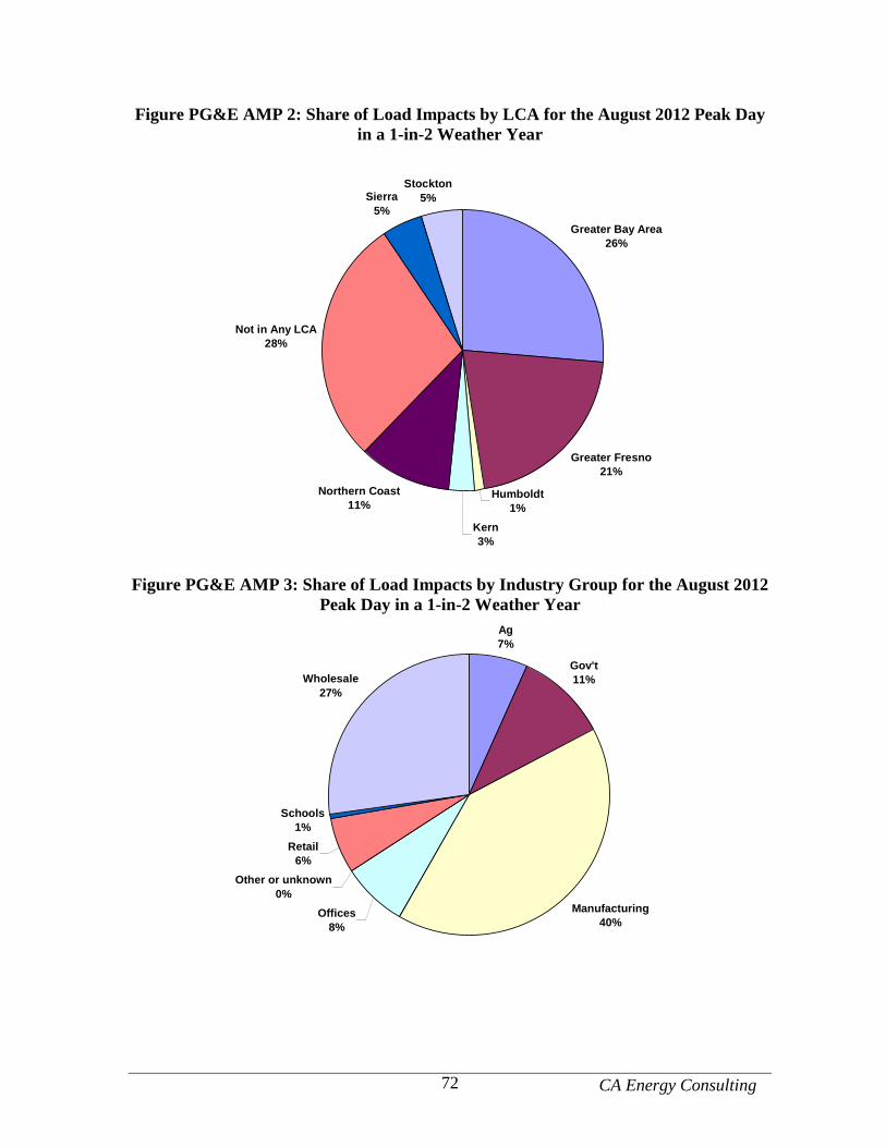
CA Energy Consulting 72
Figure PG&E AMP 2: Share of Load Impacts by LCA for the August 2012 Peak Day in a 1-in-2 Weather Year
Greater Bay Area 26%
Greater Fresno 21%
Humboldt 1%
Kern 3%
Northern Coast 11%
Not in Any LCA28%
Sierra 5%
Stockton 5%
Figure PG&E AMP 3: Share of Load Impacts by Industry Group for the August 2012
Peak Day in a 1-in-2 Weather Year Ag7%
Gov't11%
Manufacturing40%
Offices8%
Other or unknown0%
Retail6%
Schools1%
Wholesale27%
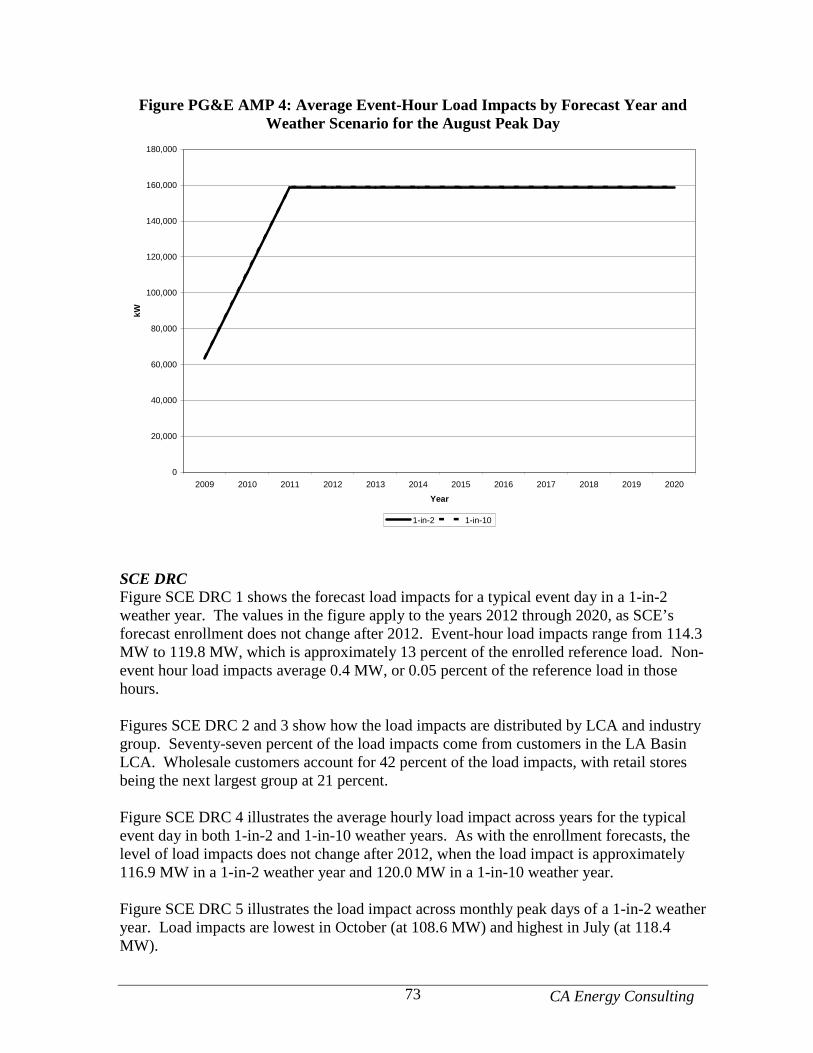
CA Energy Consulting 73
Figure PG&E AMP 4: Average Event-Hour Load Impacts by Forecast Year and Weather Scenario for the August Peak Day
0
20,000
40,000
60,000
80,000
100,000
120,000
140,000
160,000
180,000
2009 2010 2011 2012 2013 2014 2015 2016 2017 2018 2019 2020
Year
kW
1-in-2 1-in-10
SCE DRC Figure SCE DRC 1 shows the forecast load impacts for a typical event day in a 1-in-2 weather year. The values in the figure apply to the years 2012 through 2020, as SCE’s forecast enrollment does not change after 2012. Event-hour load impacts range from 114.3 MW to 119.8 MW, which is approximately 13 percent of the enrolled reference load. Non-event hour load impacts average 0.4 MW, or 0.05 percent of the reference load in those hours. Figures SCE DRC 2 and 3 show how the load impacts are distributed by LCA and industry group. Seventy-seven percent of the load impacts come from customers in the LA Basin LCA. Wholesale customers account for 42 percent of the load impacts, with retail stores being the next largest group at 21 percent. Figure SCE DRC 4 illustrates the average hourly load impact across years for the typical event day in both 1-in-2 and 1-in-10 weather years. As with the enrollment forecasts, the level of load impacts does not change after 2012, when the load impact is approximately 116.9 MW in a 1-in-2 weather year and 120.0 MW in a 1-in-10 weather year. Figure SCE DRC 5 illustrates the load impact across monthly peak days of a 1-in-2 weather year. Load impacts are lowest in October (at 108.6 MW) and highest in July (at 118.4 MW).
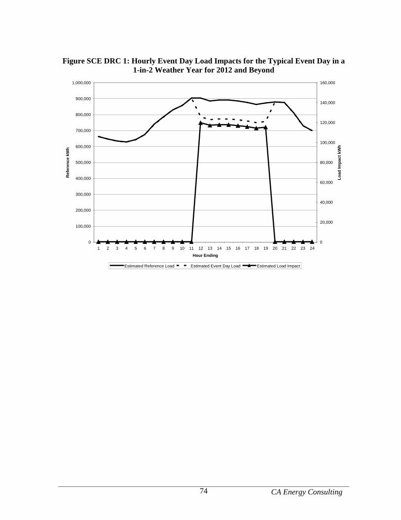
CA Energy Consulting 74
Figure SCE DRC 1: Hourly Event Day Load Impacts for the Typical Event Day in a
1-in-2 Weather Year for 2012 and Beyond
0
100,000
200,000
300,000
400,000
500,000
600,000
700,000
800,000
900,000
1,000,000
1 2 3 4 5 6 7 8 9 10 11 12 13 14 15 16 17 18 19 20 21 22 23 24
Hour Ending
Ref
eren
ce k
Wh
0
20,000
40,000
60,000
80,000
100,000
120,000
140,000
160,000
Load
Impa
ct k
Wh
Estimated Reference Load Estimated Event Day Load Estimated Load Impact
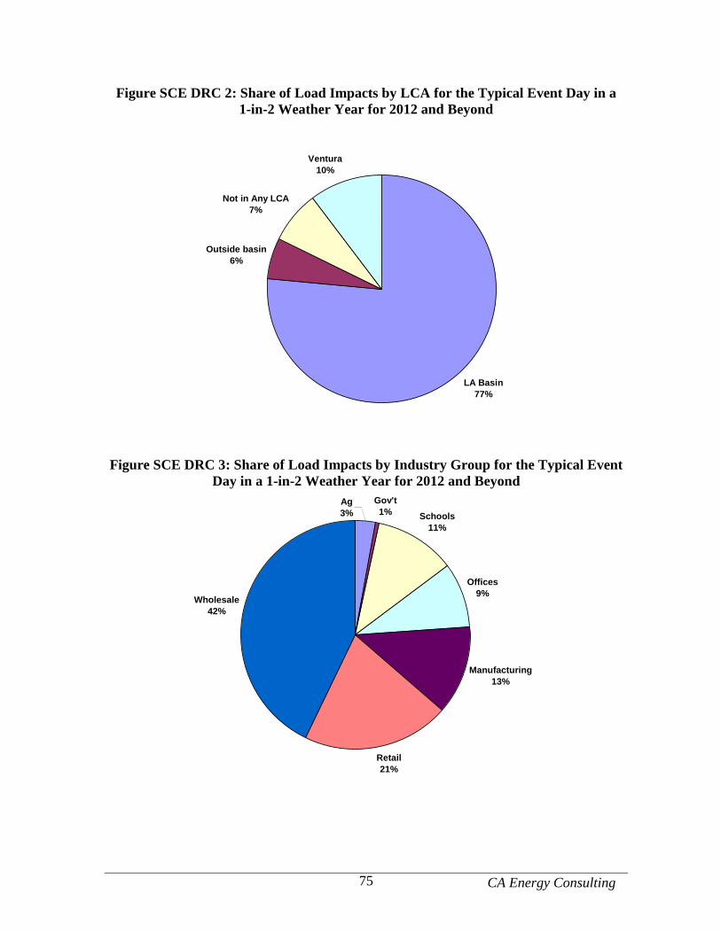
CA Energy Consulting 75
Figure SCE DRC 2: Share of Load Impacts by LCA for the Typical Event Day in a 1-in-2 Weather Year for 2012 and Beyond
LA Basin77%
Outside basin6%
Not in Any LCA7%
Ventura10%
Figure SCE DRC 3: Share of Load Impacts by Industry Group for the Typical Event
Day in a 1-in-2 Weather Year for 2012 and Beyond Gov't1% Schools
11%
Offices9%
Manufacturing13%
Retail21%
Wholesale42%
Ag3%
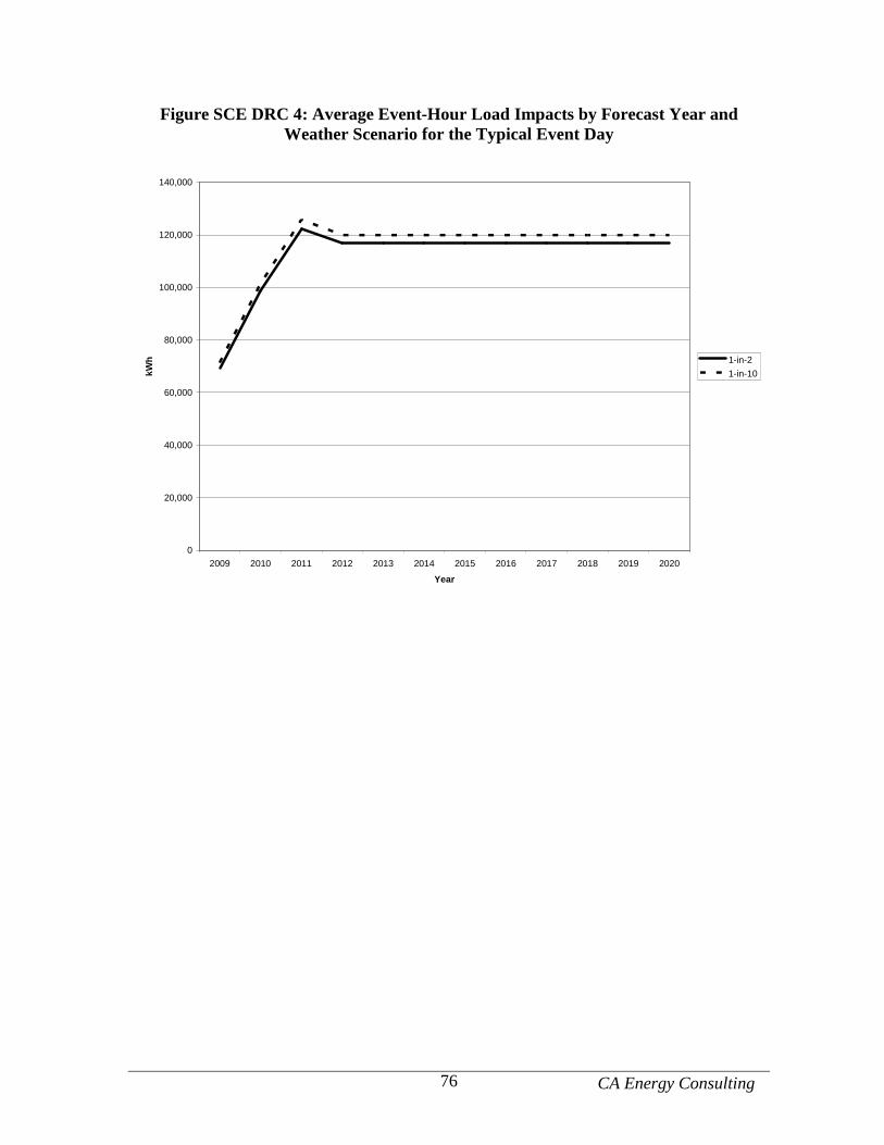
CA Energy Consulting 76
Figure SCE DRC 4: Average Event-Hour Load Impacts by Forecast Year and Weather Scenario for the Typical Event Day
0
20,000
40,000
60,000
80,000
100,000
120,000
140,000
2009 2010 2011 2012 2013 2014 2015 2016 2017 2018 2019 2020
Year
kWh 1-in-2
1-in-10
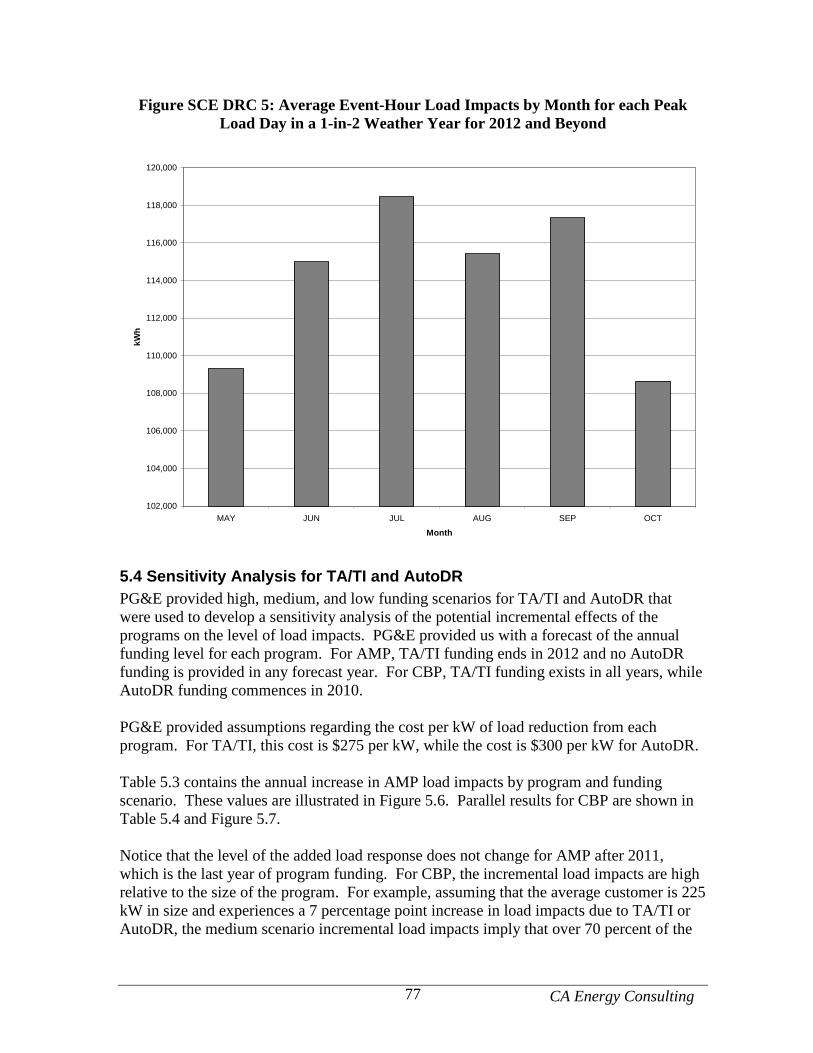
CA Energy Consulting 77
Figure SCE DRC 5: Average Event-Hour Load Impacts by Month for each Peak Load Day in a 1-in-2 Weather Year for 2012 and Beyond
102,000
104,000
106,000
108,000
110,000
112,000
114,000
116,000
118,000
120,000
MAY JUN JUL AUG SEP OCT
Month
kWh
5.4 Sensitivity Analysis for TA/TI and AutoDR PG&E provided high, medium, and low funding scenarios for TA/TI and AutoDR that were used to develop a sensitivity analysis of the potential incremental effects of the programs on the level of load impacts. PG&E provided us with a forecast of the annual funding level for each program. For AMP, TA/TI funding ends in 2012 and no AutoDR funding is provided in any forecast year. For CBP, TA/TI funding exists in all years, while AutoDR funding commences in 2010. PG&E provided assumptions regarding the cost per kW of load reduction from each program. For TA/TI, this cost is $275 per kW, while the cost is $300 per kW for AutoDR. Table 5.3 contains the annual increase in AMP load impacts by program and funding scenario. These values are illustrated in Figure 5.6. Parallel results for CBP are shown in Table 5.4 and Figure 5.7. Notice that the level of the added load response does not change for AMP after 2011, which is the last year of program funding. For CBP, the incremental load impacts are high relative to the size of the program. For example, assuming that the average customer is 225 kW in size and experiences a 7 percentage point increase in load impacts due to TA/TI or AutoDR, the medium scenario incremental load impacts imply that over 70 percent of the
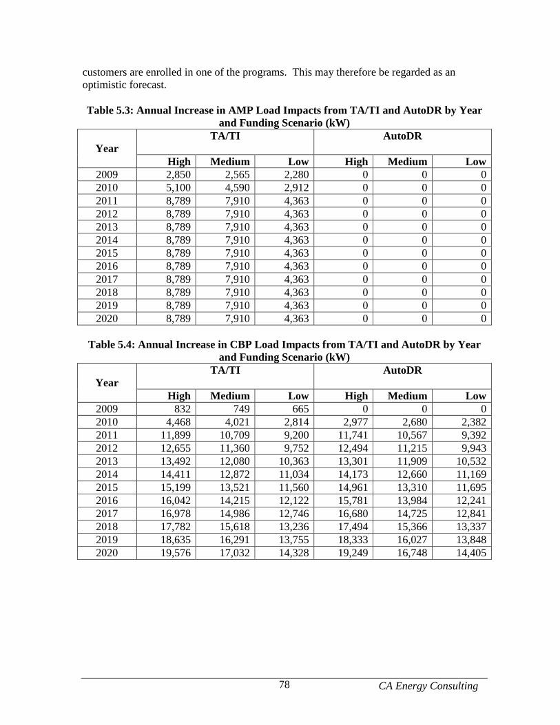
CA Energy Consulting 78
customers are enrolled in one of the programs. This may therefore be regarded as an optimistic forecast. Table 5.3: Annual Increase in AMP Load Impacts from TA/TI and AutoDR by Year
and Funding Scenario (kW) TA/TI
AutoDR
Year High Medium Low High Medium Low
2009 2,850 2,565 2,280 0 0 0 2010 5,100 4,590 2,912 0 0 0 2011 8,789 7,910 4,363 0 0 0 2012 8,789 7,910 4,363 0 0 0 2013 8,789 7,910 4,363 0 0 0 2014 8,789 7,910 4,363 0 0 0 2015 8,789 7,910 4,363 0 0 0 2016 8,789 7,910 4,363 0 0 0 2017 8,789 7,910 4,363 0 0 0 2018 8,789 7,910 4,363 0 0 0 2019 8,789 7,910 4,363 0 0 0 2020 8,789 7,910 4,363 0 0 0
Table 5.4: Annual Increase in CBP Load Impacts from TA/TI and AutoDR by Year
and Funding Scenario (kW) TA/TI
AutoDR
Year High Medium Low High Medium Low
2009 832 749 665 0 0 0 2010 4,468 4,021 2,814 2,977 2,680 2,382 2011 11,899 10,709 9,200 11,741 10,567 9,392 2012 12,655 11,360 9,752 12,494 11,215 9,943 2013 13,492 12,080 10,363 13,301 11,909 10,532 2014 14,411 12,872 11,034 14,173 12,660 11,169 2015 15,199 13,521 11,560 14,961 13,310 11,695 2016 16,042 14,215 12,122 15,781 13,984 12,241 2017 16,978 14,986 12,746 16,680 14,725 12,841 2018 17,782 15,618 13,236 17,494 15,366 13,337 2019 18,635 16,291 13,755 18,333 16,027 13,848 2020 19,576 17,032 14,328 19,249 16,748 14,405
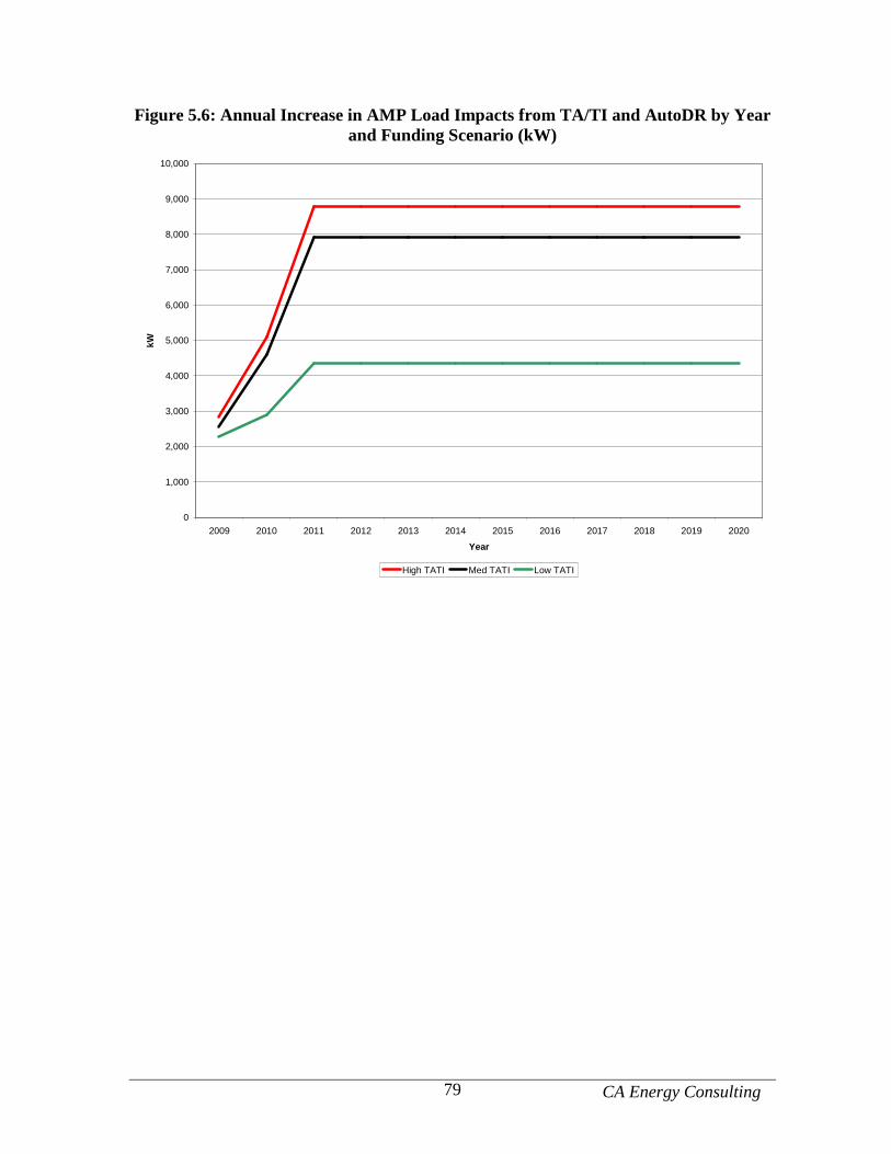
CA Energy Consulting 79
Figure 5.6: Annual Increase in AMP Load Impacts from TA/TI and AutoDR by Year and Funding Scenario (kW)
0
1,000
2,000
3,000
4,000
5,000
6,000
7,000
8,000
9,000
10,000
2009 2010 2011 2012 2013 2014 2015 2016 2017 2018 2019 2020
Year
kW
High TATI Med TATI Low TATI
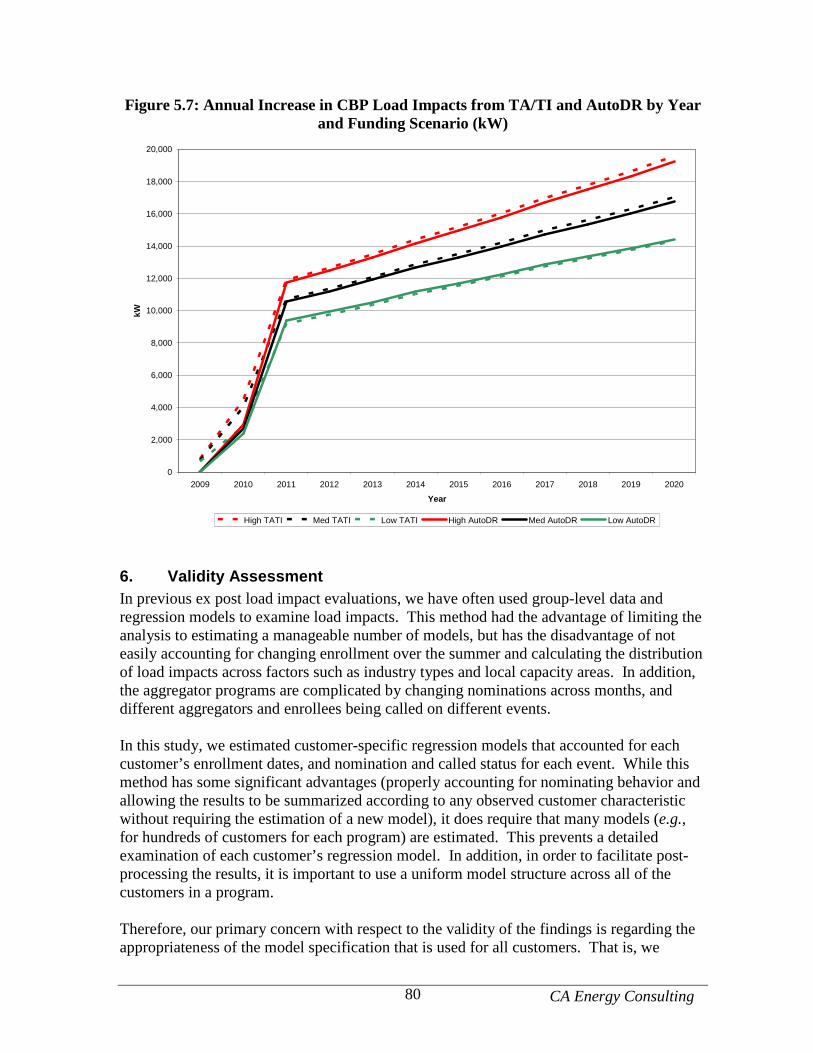
CA Energy Consulting 80
Figure 5.7: Annual Increase in CBP Load Impacts from TA/TI and AutoDR by Year and Funding Scenario (kW)
0
2,000
4,000
6,000
8,000
10,000
12,000
14,000
16,000
18,000
20,000
2009 2010 2011 2012 2013 2014 2015 2016 2017 2018 2019 2020
Year
kW
High TATI Med TATI Low TATI High AutoDR Med AutoDR Low AutoDR
6. Validity Assessment In previous ex post load impact evaluations, we have often used group-level data and regression models to examine load impacts. This method had the advantage of limiting the analysis to estimating a manageable number of models, but has the disadvantage of not easily accounting for changing enrollment over the summer and calculating the distribution of load impacts across factors such as industry types and local capacity areas. In addition, the aggregator programs are complicated by changing nominations across months, and different aggregators and enrollees being called on different events. In this study, we estimated customer-specific regression models that accounted for each customer’s enrollment dates, and nomination and called status for each event. While this method has some significant advantages (properly accounting for nominating behavior and allowing the results to be summarized according to any observed customer characteristic without requiring the estimation of a new model), it does require that many models (e.g., for hundreds of customers for each program) are estimated. This prevents a detailed examination of each customer’s regression model. In addition, in order to facilitate post-processing the results, it is important to use a uniform model structure across all of the customers in a program. Therefore, our primary concern with respect to the validity of the findings is regarding the appropriateness of the model specification that is used for all customers. That is, we
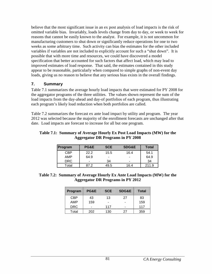
CA Energy Consulting 81
believe that the most significant issue in an ex post analysis of load impacts is the risk of omitted variable bias. Invariably, loads levels change from day to day, or week to week for reasons that cannot be easily known to the analyst. For example, it is not uncommon for manufacturing customers to shut down or significantly reduce operations for one to two weeks as some arbitrary time. Such activity can bias the estimates for the other included variables if variables are not included to explicitly account for such a “shut down”. It is possible that with more time and resources, we could have discovered a model specification that better accounted for such factors that affect load, which may lead to improved estimates of load response. That said, the estimates contained in this study appear to be reasonable, particularly when compared to simple graphs of non-event day loads, giving us no reason to believe that any serious bias exists in the overall findings.
7. Summary Table 7.1 summarizes the average hourly load impacts that were estimated for PY 2008 for the aggregator programs of the three utilities. The values shown represent the sum of the load impacts from the day-ahead and day-of portfolios of each program, thus illustrating each program’s likely load reduction when both portfolios are called. Table 7.2 summarizes the forecast ex ante load impact by utility and program. The year 2012 was selected because the majority of the enrollment forecasts are unchanged after that date. Load impacts are forecast to increase for all but one program.
Table 7.1: Summary of Average Hourly Ex Post Load Impacts (MW) for the Aggregator DR Programs in PY 2008
Program PG&E SCE SDG&E Total
CBP 22.2 15.5 16.4 54.1AMP 64.9 - - 64.9DRC - 34 - 34Total 87.2 49.5 16.4 211.9
Table 7.2: Summary of Average Hourly Ex Ante Load Impacts (MW) for the
Aggregator DR Programs in PY 2012
Program PG&E SCE SDG&E Total
CBP 43 13 27 83 AMP 159 - - 159 DRC - 117 - 117 Total 202 130 27 359


![Danielle lovelace[1]](https://img.pdfslide.us/doc/110x75/547b72efb4af9fbe158b4f8b/danielle-lovelace1.jpg)