Embed Size (px)
Citation preview

8/2/2019 2007_A Behavioral Model for Stock Prices
http://slidepdf.com/reader/full/2007a-behavioral-model-for-stock-prices 1/42
Contemporary Issues and Ideas in Social Sciences
August 2007
A Behavioral Model For Stock Prices
N. Lalitha1
Department of Economics, Shyama Prasad Mukherjee College,University of Delhi, New Delhi 110026, India
D. N. Rao
Centre for Economic Studies and Planning, School of Social Sciences,Jawaharlal Nehru University, New Delhi 110067, India
Abstract
Multi-factor models have been popularly used to explain asset market behavior. The Famaand French three-factor model fitted on the sample set of new economy stocks for the studyperiod of late nineties to early 2000s, however, fails to give adequate explanation of thestock market behavior. A behavioral model built on the assumption of bounded rationality
and biases in investor behavior seems to offer a better explanation of the stock price behavior.
JEL Classification: G12
1For Correspondence: Email: lalitha [email protected]

8/2/2019 2007_A Behavioral Model for Stock Prices
http://slidepdf.com/reader/full/2007a-behavioral-model-for-stock-prices 2/42
2 CIISS August 2007
INTRODUCTION
Tracing stock price movements is a difficult exercise that involves detailed examinationof firm specific and industry specific factors. It is now widely recognized that Sharpe (1964)
and Lintner (1965) and Mossin’s (1966) Capital Asset Pricing Model (CAPM) and its othervariants do not adequately describe the cross section of expected returns. Investors havebeen found to earn abnormal returns in excess of those predicted by the model. We there-fore developed a simple model for stock price movement that incorporates investor behaviorpattern. By examining the stock price data of a sample set of technology, media and telecom(TMT) companies, listed in the Bombay Stock Exchange, during the late 90’s and early 2000period we identified inertia in investor behavior as an important factor in generating mar-ket fads. The hype associated with all sorts of dot-com and media companies that pushedstock markets worldwide during the later part of nineties and early two thousand poses aninteresting question as to whether such boom in technology and media stocks was justifiedby fundamentals or was it a mere fad? Using the behavioral inertia approach, the present
study tries to show that the market was indeed driven by the craze surrounding such stocks.The paper is divided into three broad sections. In section 1 we introduce asset pricing
models. A brief description of Fama and French three factor model is followed by its empiricalinvalidation using the sample data under consideration. In section 2 the drawbacks of the neo-classical approach -the framework within which most asset pricing models are constructed–is highlighted. A behavioral stock price model that incorporates investor behavior patternand is less restrictive in assumptions has been proposed. The result of an empirical test of the model is also examined in this section. In section 3 a comparative evaluation of the twomodels is done by looking at their forecasting power.
1 Asset Pricing Models
The Capital Asset Pricing Model (CAPM) is one of the most extensively studied modelsboth theoretically and empirically for valuation of securities. The CAPM is a theory aboutthe way stocks are priced in relation to their risk. The underlying logic of the theory is thatassets with the same risk should earn the same expected returns. The CAPM puts forwardthe idea that in market equilibrium assets earn premia over the riskless rate that increaseswith their risk, where the determining influence on risk premia is the covariance betweenthe asset and the so called market portfolio- the ‘β ’ of the asset, rather than the own orintrinsic risk of an asset. Various versions of CAPM are available in the literature whichwere built by relaxing some of the stringent assumptions of the original model. However,starting in the late 1970s empirical work appeared that challenged even the robust version of
the CAPM. Fama and French (1992) made a devastating blow to CAPM when they reportedthat there seemed to be no connection between beta and returns. Fama and French arguedthat the higher average return on small stocks and high book-to-market value stocks reflectunidentified state variables that produce undiversifiable risks (covariances) in returns thatare not captured by market returns and are priced separately from market betas. Fama andFrench (1996) therefore formulated an extension of the CAPM model that describes asset

8/2/2019 2007_A Behavioral Model for Stock Prices
http://slidepdf.com/reader/full/2007a-behavioral-model-for-stock-prices 3/42
Lalitha & Rao: Stock Price Model 3
return as a function of three different sources of risk. This model explains many of theCAPM average return anomalies. In the three-factor model developed by Fama and French,size and ratio of book value of common equity to market equity (BE/ME) are used as proxy
for sensitivity to common risk factors in returns. The model described expected return on aportfolio in excess of the risk-free rate as a function of: (i) excess return on a broad marketportfolio Rm − Rf ; (ii) the difference between the return on a portfolio of small stocks andthe return on a portfolio of large stocks (SMB); and (iii) the difference between the returnon a portfolio of high BE/ME stocks and the return on a portfolio of low BE/ME stocks(HML). In other words, the expected return on portfolio i is
E(Ri) −Rf = bi[E (RM ) −Rf ] + siE (SMB) + hiE (HML)........(1)
where E (RM ) − Rf , E(SMB), E(HML) are expected premiums and the factor sensitivitiesand bi, si and hi are the slopes in the time series regression
Ri−Rf = ai + bi(RM −Rf ) + si SMB + hiHML + εi ........(2)
The study showed that the three-factor model gives a good description of returns in portfoliosformed on earnings/price (EPS/P), cash flow/price and sales growth in addition to explaining
returns on portfolios formed on size, BE/ME and industry returns.
1.1 Empirical estimation of Fama and French three-factor model
The study period covered was April 1999 to November 2004. From the TMT stocks underlyingthe various BSE and NSE indices only 35 companies were found to have a continuous pricedata and information on economic fundamentals of the company for the period covered underthe study. These, therefore, formed the sample for the present study. In general, stock marketstudies are done using portfolios rather than stock returns. Holding a diversified portfoliois assumed to take care of firm specific risk. In this study portfolios were constructed usingvarious criteria (see Appendix 1). In the Fama and French model firms with high BE/MEvalue are treated as weak firms experiencing distress. The risk associated with such firms
gets priced and is reflected in high returns and positive∧
hi. On the other hand, firms with low
BE/ME values are strong firms and have negative loading on∧
hi. Similarly, small firms havelow earnings on assets and are less profitable than big firms. So size is treated as a proxy forrisk factor and therefore small firms will have higher expected returns and positive slope on

8/2/2019 2007_A Behavioral Model for Stock Prices
http://slidepdf.com/reader/full/2007a-behavioral-model-for-stock-prices 4/42
4 CIISS August 2007
SMB as against big firms which have lower expected returns and negative slope SMB. Aftertesting for stationarity (see Appendix 2) the model is estimated by running the regressionequation (2) and validated by testing for H o : ai = 0. We estimated this regression for the
thirty-six constructed portfolios (see Table 1 and Table 2). A detailed analysis of Table 1showed that:
1. For the six equal weighted size-BE/ME portfolios, the H o : ai = 0 is accepted. Thenull, however, does not hold for value weighted size-BE/ME (except SMBEME) as alsofor single sort BE/ME (both equal and value weighted) portfolios evaluated at 5% levelof significance.
2. As compared to value weighted portfolios, equal weighted portfolios seem to have bothbetter explanatory power, as also greater sensitivity to size and BE/ME factors.
3. Slope on SMB is high and strong in the small category for both equal and value weighted
portfolios. In the big group SMB is not only small in magnitude but also insignificant.Also, the slope coefficient is positively related to returns in some categories. Similarlywhen ranking is on the basis of BE/ME alone, SMB is significant for equal weightedcategory and not for value weighted category.
4. Loadings on HML on all the portfolios is strongly supported in all except SMBEME(both equal and value weighted) and SHBEME value weighted stocks. In all the regres-sions low BE/ME stocks have negative coefficients whereas high BE/ME stocks havepositive coefficients.
5. The explanatory power of regression is good when the BE/ME criteria is used alonefor constructing portfolios. Combined with size the regression works well for small as
against big. Equal weighted portfolios seem to do better than value weighted.
Thus, the high R2 associated with the above regression indicates that there is risk related tosize and BE/ME which captures common variation in returns. However, whereas the modelpicks up the premium associated with small size when in the first place small size is alreadyhighlighted, it fails to establish a discount in returns for big sized firms. It however, pricesthe risk captured by BE/ME factor along the predicted lines of the model. Thus the sizepremium is weaker and less reliable than the value premium.
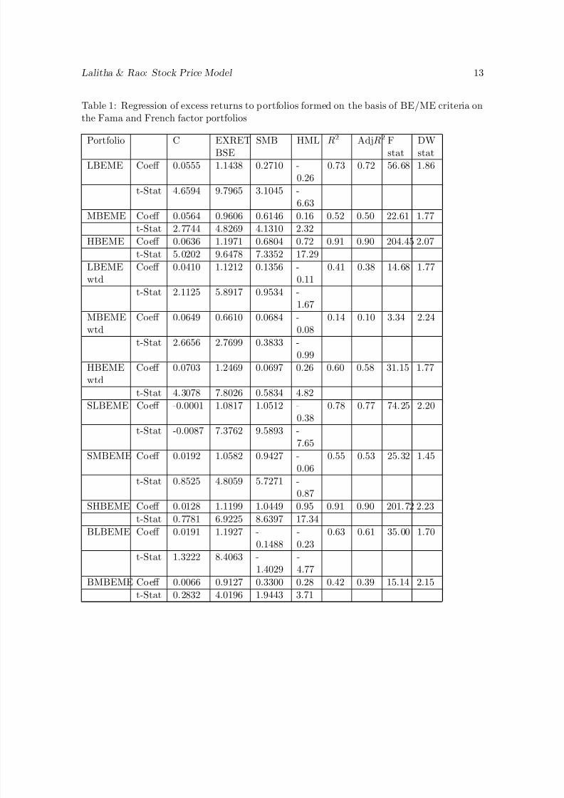
EPS/P Criteria The regression estimates of equation (2) using portfolios constructed on
the basis of EPS/P ranking also shows poor performance of the multifactor model. In bothequal and value weighted double sort category for only 3 out of 6 portfolios, the three-factormodel fails to reject the H o. In the single sort category again for only portfolios LEPSand LEPS weighted the H o is not rejected again evaluated at 5% level of significance. Theslope coefficients on SMB and HML also do not conform to the three-factor model. None of the low EPS/P portfolios have a negative loading on HML. Similarly in the big size-EPS/P

8/2/2019 2007_A Behavioral Model for Stock Prices
http://slidepdf.com/reader/full/2007a-behavioral-model-for-stock-prices 5/42
Lalitha & Rao: Stock Price Model 5
category none have significant SMB and only 2 out of 6 big-size portfolios have negativecoefficient on SMB. The insipid performance of the model when portfolios are formed usingEPS/P criteria indicates that the earnings variable does not adequately capture information
regarding returns in stock prices. Further, the weak correlation between BE/ME and EPS/Pfor sample companies (a meagre 0.19) implies that earnings variable also fails to pick-up therisk associated with high BE/ME firms. Thus, the empirical exercise showed that the modelperformed somewhat better when portfolios were constructed using BE/ME criteria. Thiswas not surprising considering the fact that the risk mimicking portfolios SMB and HMLwere themselves formed on the basis of size and BE/ME ranking. They would therefore beable to explain return on other portfolios formed on similar ranking. Thus the validity of the Fama and French model is dependent upon the criteria used for constructing sampleportfolios as also the risk mimicking portfolios. A more serious problem facing the Fama andFrench model is its failure to explain the momentum effect, (which argues that past relativeperformance predicts future relative performance) of Jegadeesh and Titman (1993).
2 Drawbacks of neoclassical approach
The results of Fama and French model challenge us with a need to develop an alternatemodel for stock market behavior in the late 1990s and early 2000. The rise in stock pricesnot justified by fundamentals directs us into the realm of behavioral inertia. The Fama andFrench model, built in the neo-classical framework, has great theoretical appeal but limitedempirical relevance. The neo-classical approach imposes stringent assumption on the behaviorof economic agents. The assumption of perfect rationality, for example, has come in for a lotof criticism. It is now recognized that individuals at best have imperfect rationality. Withlimited time, brainpower and bounded rationality individuals are often not in a positionto maximize their objective function and would instead settle for a ‘satisfactory’ level of the target variable. Moreover even the ‘optimum’ level so identified may not be chosen foraltruistic reasons. With these modified assumptions it is no longer certain that equilibriumvalues would be achieved. In the capital market, for instance, while the trading by rationaltraders traces the path towards equilibrium, trading activities of irrational traders pushesthe market away from the equilibrium point. The equilibrium prices are a weighted averageof the beliefs of rational and irrational traders, and the influence of either group on pricesdepends upon their risk bearing capacity. Arbitrage will, therefore, not eliminate mispricing.Arbitraging does not work efficiently, since it is hard for an investor to know whether otherinvestors have yet detected and acted upon it.
Persistent mispricing might also occur because some relevant piece of public information
is either ignored or misused by everyone leading to market prices being regularly at odds withfundamental values. All individuals have biases especially under conditions when informationis slack. While it might be argued that in the modern day computerized world, informationis no longer a constraint, the question of quality of information, its proper interpretationand analyses still remains. And since individuals have similar biases, it will be incorrectto assume that errors cancel out in equilibrium and therefore that the estimated values will

8/2/2019 2007_A Behavioral Model for Stock Prices
http://slidepdf.com/reader/full/2007a-behavioral-model-for-stock-prices 6/42
6 CIISS August 2007
approximate the true values. Neoclassical economists arguing for the existence of equilibriumhad immense faith in human learning capabilities and therefore believed that individuals willnot systematically and consistently make the same mistake. However, experimentation liter-
ature has shown that there can be a complete lack of learning even in infinite horizons. Sincethere are some opportunity costs to learning, even a completely ‘rational’ learner will chosenot to experiment and remain in a non-optimal equilibrium if the cost of trying somethingelse is too high. Moreover, the time required to converge to an equilibrium strategy can beextremely long, especially in a situation of changing environment. Thus, markets can be ina situation of perpetual non-convergence.
2.1 Behavioral inertia model for stock prices
Faced with information, time and resource constraints and also a stock price series that ex-
hibits random walk, investors find that the best forecast of the future price is in fact thecurrent price. In an uncertain world, where information is revealed through a sequence of events, the cost of collecting and analyzing information are exorbitant in terms of money,time and expertise. Market participants will therefore find it more ‘rational’ and practical tochange their decisions only slowly even when underlying economic conditions are constantlychanging. Thus, they would find greater returns with inaction rather than optimizing actionand behavioral inertia plays the important role of imparting stability in individual’s behav-ior. Inertia produces highly auto-correlated time series in which random events have lastingeffects.
The behavioral inertia approach has been shown to be a combination of inertia andcaprice, i.e. random change (Stanley 2000). Individuals are often overconfident about theirabilities and therefore may deviate from the tried and tested path. Such ‘irrationality’ inbehavior creates uncertainity in all economic phenomena. Caprice provides a mechanismof behavioral variation, which promotes advancement of the society. It also exhibits inertiaor pattern in variation. Variations that were successful in the most recent past will tendto remain successful in the near future as well, implying positive autocorrelations amongthe innovations. By explicitly identifying inertia and caprice, the Behavioral Inertia Modelproposes a dynamic theory of economic phenomena. The idea that the current price is thebest predictor of future price has been quite popular both with lay investors as well as aca-demicians. Proponents of Efficient Market Hypothesis (weak form) treat current price asreflecting all the information that is contained in past prices. They therefore, highlight thefutility of forming trading rules based on share price history. Keynes (1936) argued thatinvestors accept current valuations as a correct reflection of the market assessment of future
prospects. They downplay the fact that these valuations can be incorrect. Faced with un-certainty regarding factors that might affect stock prices market participants seek safety byconforming to the behavior of the majority on the average. This however, does not rule outthe possibility of profit making by predicting changes in the conventional basis of valuation,a short time ahead of the rest of the investor population. Such a possibility generates spec-ulative behavior amongst investors. In the literature on finance it is common to find lagged

8/2/2019 2007_A Behavioral Model for Stock Prices
http://slidepdf.com/reader/full/2007a-behavioral-model-for-stock-prices 7/42
Lalitha & Rao: Stock Price Model 7
dependent variables when stock market analysis is in the returns framework (e.g. Fama andFrench (1988)). There are also studies on asset market that include time dependency inpreferences in utility function. These, however, are built in the neoclassical framework and
incorporate habit persistence in consumption in the utility function. Constandinides(1988),Detemple(1989), Heaton(1989) and Sunderasan(1989) examined asset pricing on the basis of habit formation. Heaton(1995) used a simulated Method of Moments approach to evaluate arepresentative consumer asset pricing model and reported evidence for the local substitutionof consumption with habit formation occurring over longer periods of time. By incorporatingsuch time non-separability in preferences, the performances of asset pricing models have beenfound to improve. The behavioral inertia model that we developed is not based on optimiz-ing principles. Ours is a simple approach that allows for biases in individual behavior andtreats them as incompletely rational. Therefore, our approach does not entail calculations of rationally expected returns, which in any case cannot be calculated in ex- ante terms. In thisstudy, we developed a behavioral inertia model at the stock level rather than at the portfolio
level. This is owing to the fact that investors rarely hold a well diversified portfolio (see Bar-ber and Odean (2000); Polkovinchenko (2003); Goetzmann and Kumar (2004)). Investors’personal characteristics, their stock preferences and their behavioral biases jointly influencetheir diversification choices (Goetzmann and Kumar (2004), Kumar & Lim (2004)). Huber-man(2001) also reported the tendency of household investments to be primarily concentratedin their employer’s stocks and in general in stocks of companies registered in their country asagainst foreign company stocks. These phenomena provide compelling evidence that peopleinvest in the familiar stocks while often ignoring the principles of portfolio theory. Further,by working directly with prices rather than stock returns one can draw unambiguous con-clusions. With returns, a choice between equal weighted versus value weighted returns hasdifferent implications for the behavior of the stock markets. More importantly, by working
with prices rather than returns, we avoid the crucial question of unit of time for returns.Measurement choice between average monthly abnormal returns vis--vis buy and hold ab-normal returns has severe effect on the outcome of the study. Choice of a normal period toestimate a stock’s expected return is also problematic as stocks can show return continuationin the short run and mean reversion in the long-run.
2.2 The Model
We capture the inertia in stock prices and the market dynamism by formulating an assetpricing model as a function of lagged prices and C t the caprice element.Assuming inertial decay
Pt = α0 P α1t−1C t ........ (3)
If caprice also experiences the same type of exponential decay then

8/2/2019 2007_A Behavioral Model for Stock Prices
http://slidepdf.com/reader/full/2007a-behavioral-model-for-stock-prices 8/42
8 CIISS August 2007
Ct = X β t C
ρt−1 t........ (4)
whereX t is 1 x k vector of explanatory variables,
β is a k x 1 vector of regression coefficients.ρ is the auto-regression coefficient for caprice, a measure of its persistence and t is the truly
random irreducibly stochastic past. Re-writing the above equations in logarithmic form, weget
lnP t = lnα0 +α1 lnP t−1 + lnC t ........ (5)
lnC t = β lnX t + ρ lnC t−1 + ln εt ........(6)
and further
lnC t−1 = lnP t−1− lnα0−α1 lnP t−2 ........(7)
Thus, for each stock i,
lnP it = lnα0i +α1i lnP it−1 +β i lnX it + ρi [lnP it−1− lnα0i−αi1 lnP it−2] + ln εit
or
lnP it = lnα0i + (α1i + ρi) lnP it−1 +β i lnX it− ρi lnα0i− ρi α1i lnP it−2 + ln εit
or
lnP it = (1 − ρi) lnα0i + (α1i + ρi) lnP it−1− ρi α1i lnP it−2
+ β 1i lnX 1it +β 2i lnX 2it +β 3i lnX 3it +β 4i lnX 4it + ln εit ........ (8)
(obtained by decomposing X it into its components) Thus, the testing of the model involvesrunning the following regression
lnP it = (1 − ρi) lnα0i + (α1i + ρi) lnP it−1− ρi α1i lnP it−2
+ β 1i lnX 1it +β 2i lnX 2it +β 3i lnX 3it +β 4i lnX 4it + ν t ........ (9)
where ν t = ln εit
The presence of inertia is ascertained by testing for the
H0 : (α1i + ρi) − ρi α1i = 1
i.e. sum of AR(autoregressive) coefficients = 1

8/2/2019 2007_A Behavioral Model for Stock Prices
http://slidepdf.com/reader/full/2007a-behavioral-model-for-stock-prices 9/42
Lalitha & Rao: Stock Price Model 9
2.3 Empirical Testing of the Model
In our exercise the explanatory variables included are natural log of book-to-market value
(lnB/M), natural log of market value (lnMV) and natural log of beta (lnbeta). Of the 35stocks 3 stocks namely ASM Tech, BPL and Nelco had negative BE/ME value and weretherefore dropped. Many of the stocks reported negative beta values for part of the timeperiod under consideration. Moreover, the coefficient of beta was found to be insignificant ina preliminary exercise of univariate regression using cross-section data. However, consideringthe fact that for long, beta dominated the risk-return models, we saw it reasonable to continueincluding beta in the set of explanatory variables. To take care of the problem of findingnatural log for negative betas we bifurcated the beta variable into lnβ positive and lnβ negative. For positive beta values natural log is estimated and is recorded as variable lnbetapositive. For such periods with positive beta, the variable lnbeta negative shows the valueof zero. Similarly, for negative betas, the ln value of |β |is estimated (i.e. excluding negative
sign) and this is treated as variable lnβ negative. Here the variable lnβ positive has elementszero for the corresponding time period. Out of the thirty-two sample companies thirteen hadtwo beta variables of lnbeta and lnbeta negative. The results of ADF test on all the variablesused in the model (given in Appendix 3) show that only for the ln price series the null of Unit root with trend and intercept is not accepted at 5% (though not rejected at 1%) for asmall number of companies. The p values of the likelihood ratio test of the coefficient on theone time lag of the dependent variable and the trend being jointly equal to zero shows thatfor Afte, Crest, DSQ, Eserve, Hinduja, InfoSys, Moser, MTNL, Orient, Penasoft, TataElxsiand Vindhyas the absence of trend is accepted at 1% but not at the 5% level of significance.Similarly, the presence of Unit root with intercept alone is not accepted by lnprice series of Eserve, Hinduja and Moser at 5% level of significance.
For all other series the null hypothesis of Unit root is accepted with trend alone at 5%level of significance.
After ascertaining the independence of the error terms (see Appendix 4) we estimated themodel by running the following regression on price series of nineteen companies which hadpositive beta values throughout the study period.
lnP t = β 0 +β 1 lnP t−1 +β 2 lnP t−2 +β 3 lnBM + β 4 lnMV + β 5 ln beta + ν t
For the thirteen companies which had negative betas for part of the sample period thebeta dummy of lnbeta negative was included in the above regression. Thus, the followingregression was run.
lnP t = β 0 +β 1 lnP t−1 +β 2 lnP t−2 +β 3 lnBM + β 4 lnMV + β 5 lnbeta+ β 6 ln betaneg + ν t
The results of the above regression are reported in Table 3. The last column of the Tablegives us the ‘t’ values calculated for the null hypothesis of
β 1 +β 2 = 1

8/2/2019 2007_A Behavioral Model for Stock Prices
http://slidepdf.com/reader/full/2007a-behavioral-model-for-stock-prices 10/42

8/2/2019 2007_A Behavioral Model for Stock Prices
http://slidepdf.com/reader/full/2007a-behavioral-model-for-stock-prices 11/42
Lalitha & Rao: Stock Price Model 11
Moreover as suggested by Daniel and Titman(1997), characteristics could have informationindependent of the covariance structure of returns that helps explain expected portfolio re-turns. To understand the implications of these two approaches we undertook a comparative
evaluation of the multifactor model and the behavioral model. Though the two models differin terms of the dependent variable, they can still be compared on the basis of their predictivepower. A dynamic, in-sample forecast using forecasted values for lagged dependent variableswas done for the two models viz, Fama and French model and the behavioral model (seeTables 5 and 6). The Tables report two statistics- Mean Absolute Percentage Error (MAPE)and Theil’s inequality coefficient, where,
MAPE is defined as 1
T
T t=1
∧Y t−Y tY t
and
Theil’s inequality coefficient U is given as
U = 1T T
t=1 ∧
Y t−Y t2
1
T
T t=1
∧
Y t
2
+
1
T
T t=1 Y t
2
Here,∧
Y t and Y t are the simulated and the actual values of dependent variables of the twomodels. These two measures of forecast error are invariant of the scale of the dependentvariable. The smaller the value of MAPE, the better is the forecasting ability of the model.The value of U lies between 0 and 1. A value of U=0 implies perfect fit, whereas a value of U=1 indicates that the model has no predictive value. A look at mean absolute percentageerror and Theil’s inequality shows that the behavioral inertia model gives a better descriptionof price behavior in the Indian stock market. Thus the forecasting exercise clearly suggests
the need to incorporate investor’s inertia in modeling stock prices.
4 CONCLUSIONS
The focus of this study has been on developing a behavioral model for understanding assetmarket behavior. Popular stock investment strategies are often fads based on market gener-ated data, especially share price as opposed to accounting data given in the company financialreports. Agents assume the current market valuation to be a reflection of the markets assess-ment of future prospects. Acting on the belief that prices will be what they were, investorsuse market valuation to pick stocks. Such behavior is self fulfilling and inertia becomes thebasis for the market action.
The behavioral inertia approach involves the use of a simple regression exercise. Complexeconometric techniques though highly popular generally do not serve much purpose. Re-searchers choose estimation techniques by looking at the diagnostic statistics of the model.It is however quite possible that what might apparently seem to be the problem may in factnot be so. For example, significant serial correlation in estimated residuals may be due to thepresence of ARCH effect in residuals or the omission of lagged dependent and explanatory

8/2/2019 2007_A Behavioral Model for Stock Prices
http://slidepdf.com/reader/full/2007a-behavioral-model-for-stock-prices 12/42
12 CIISS August 2007
variables. Hence a model with autocorrelation in disturbances should be developed only aftertesting for the above mentioned possibilities. Such prescreening of the model may howeverchange the distributional properties of subsequent statistical analysis, yielding statistics that
may have virtually unknown sampling properties.By assuming inertial decay we derive a log-linear model to describe stock price behavior.
The model that we have developed is guided by theory rather than an outcome of sampledata. Since no inductive searches for suitable econometric models are made, there is no pre-test bias. Any problem in empirical testing either in the form of misspecified error termsor coefficients with wrong sign is treated as evidence against the theory under examination.This is in contrast to the usual approach of modifying a model to arrive at a better fit to thedata in hand. This latter approach is not a desirable method of model building as correctionsmade by looking at apparent deviations from the assumptions may or may not eliminate theroot cause of the problem.
The Fama and French model is tested using portfolios constructed on the basis of BE/ME
and EPS/P ranking. The results show poor performance of the model in explaining averagereturns on the various constructed portfolios. In particular, in the BE/ME ranking the nullhypothesis of the three-factor portfolios being minimum variance efficient is accepted onlyfor the six size-BE/ME equal weighted portfolios, and the small and medium BE/ME valueweighted portfolios. A similar number of portfolios in the EPS/P ranking also accept thenull hypothesis.
The coefficients on SMB and HML also do not unambiguously reflect the pricing of riskassociated with small size and high book-to-market value firms.
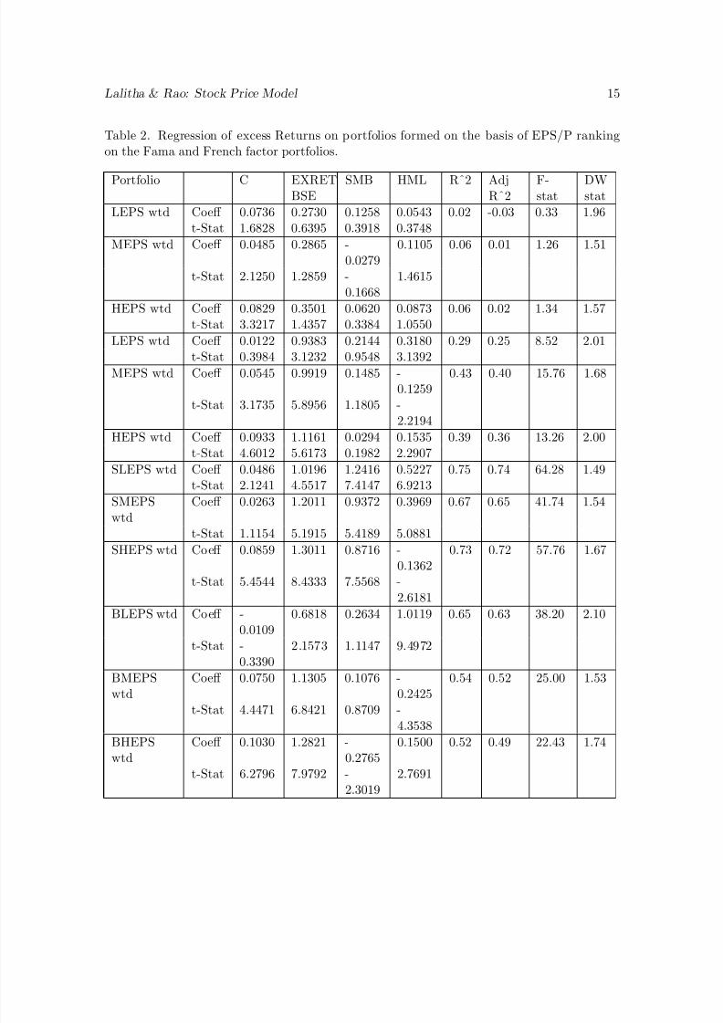
The alternate model proposed in this paper based on investor behavior pattern seems tooffer a better explanation of stock market behavior. The presence of inertia in the stock priceseries is ascertained by undertaking a ‘t’ test on the coefficients of the two lagged variables
adding up to 1. Under the condition when no distributional assumptions are made about thereturns series, an asymptotic test like Wald test would be more appropriate. We, therefore,undertook a Wald test of the null hypothesis of presence of inertia. The results of both the‘t’ test and ‘Wald’ test show that the null is not accepted in 10 out of 32 sample compa-nies, namely, Bluestar, Finolex, Jain, Mphasis, MTNL, NIIT, Satyam, TataElxsi, Wipro andZensar.
An in-sample forecasting of the two models viz. Fama and French and the behavioral in-ertia model, formulated using rational and behavioral approaches respectively, also supportedour argument for incorporating behavioral biases in investor’s behavior.
8/2/2019 2007_A Behavioral Model for Stock Prices
http://slidepdf.com/reader/full/2007a-behavioral-model-for-stock-prices 13/42
Lalitha & Rao: Stock Price Model 13
Table 1: Regression of excess returns to portfolios formed on the basis of BE/ME criteria onthe Fama and French factor portfolios
Portfolio C EXRETBSE
SMB HML R2 AdjR2 Fstat
DWstat
LBEME Coeff 0.0555 1.1438 0.2710 -0.26
0.73 0.72 56.68 1.86
t-Stat 4.6594 9.7965 3.1045 -6.63
MBEME Coeff 0.0564 0.9606 0.6146 0.16 0.52 0.50 22.61 1.77
t-Stat 2.7744 4.8269 4.1310 2.32
HBEME Coeff 0.0636 1.1971 0.6804 0.72 0.91 0.90 204.45 2.07
t-Stat 5.0202 9.6478 7.3352 17.29
LBEME
wtd
Coeff 0.0410 1.1212 0.1356 -
0.11
0.41 0.38 14.68 1.77
t-Stat 2.1125 5.8917 0.9534 -1.67
MBEMEwtd
Coeff 0.0649 0.6610 0.0684 -0.08
0.14 0.10 3.34 2.24
t-Stat 2.6656 2.7699 0.3833 -0.99
HBEMEwtd
Coeff 0.0703 1.2469 0.0697 0.26 0.60 0.58 31.15 1.77
t-Stat 4.3078 7.8026 0.5834 4.82
SLBEME Coeff -0.0001 1.0817 1.0512 -
0.38
0.78 0.77 74.25 2.20
t-Stat -0.0087 7.3762 9.5893 -7.65
SMBEME Coeff 0.0192 1.0582 0.9427 -0.06
0.55 0.53 25.32 1.45
t-Stat 0.8525 4.8059 5.7271 -0.87
SHBEME Coeff 0.0128 1.1199 1.0449 0.95 0.91 0.90 201.72 2.23
t-Stat 0.7781 6.9225 8.6397 17.34
BLBEME Coeff 0.0191 1.1927 -0.1488
-0.23
0.63 0.61 35.00 1.70
t-Stat 1.3222 8.4063 -1.4029
-4.77
BMBEME Coeff 0.0066 0.9127 0.3300 0.28 0.42 0.39 15.14 2.15
t-Stat 0.2832 4.0196 1.9443 3.71

8/2/2019 2007_A Behavioral Model for Stock Prices
http://slidepdf.com/reader/full/2007a-behavioral-model-for-stock-prices 14/42
14 CIISS August 2007
Table 1: Contd.
Portfolio C EXRET
BSE
SMB HML R2 AdjR2 F
stat
DW
statBHBEME Coeff 0.0062 1.1544 -
0.14250.45 0.73 0.72 58.00 1.49
t-Stat 0.4573 8.7359 -1.4424
10.05
SHBEMEwtd
Coeff 0.0878 2.1221 0.7963 0.04 0.50 0.48 20.96 1.86
SLBEMEwtd
Coeff 0.0498 1.1756 0.8519 -0.30
0.63 0.61 35.68 1.58
t-Stat 2.5320 6.0977 5.9110 -4.60
SMBEMEwtd
Coeff 0.0684 1.1905 1.2132 -0.10
0.39 0.36 13.57 1.59
t-Stat 1.8289 3.2503 4.4311 -0.77
t-Stat 2.4951 6.1575 3.0908 0.33
SHBEMEwtd
Coeff 0.0878 2.1221 0.7963 0.04 0.50 0.48 20.96 1.86
t-Stat 2.4951 6.1575 3.0908 0.33
BLBEMEwtd
Coeff 0.0802 1.2069 0.0551 -0.35
0.53 0.51 23.91 1.53
t-Stat 3.9560 6.0745 0.3710 -
5.16BLBEMEwtd
Coeff 0.0802 1.2069 0.0551 -0.35
0.53 0.51 23.91 1.53
t-Stat 3.9560 6.0745 0.3710 -5.16
BMBEMEwtd
Coeff 0.0652 0.7453 0.0380 -0.12
0.19 0.15 4.85 2.38
t-Stat 2.7639 3.2247 0.2197 -1.59
BHBEMEwtd
Coeff 0.0578 1.0939 -0.1367
0.17 0.43 0.40 15.97 1.87
t-Stat 3.3289 6.4316 -1.0751 2.89
8/2/2019 2007_A Behavioral Model for Stock Prices
http://slidepdf.com/reader/full/2007a-behavioral-model-for-stock-prices 15/42
Lalitha & Rao: Stock Price Model 15
Table 2. Regression of excess Returns on portfolios formed on the basis of EPS/P rankingon the Fama and French factor portfolios.
Portfolio C EXRETBSE
SMB HML Rˆ2 AdjRˆ2
F-stat
DWstat
LEPS wtd Coeff 0.0736 0.2730 0.1258 0.0543 0.02 -0.03 0.33 1.96t-Stat 1.6828 0.6395 0.3918 0.3748
MEPS wtd Coeff 0.0485 0.2865 -0.0279
0.1105 0.06 0.01 1.26 1.51
t-Stat 2.1250 1.2859 -0.1668
1.4615
HEPS wtd Coeff 0.0829 0.3501 0.0620 0.0873 0.06 0.02 1.34 1.57t-Stat 3.3217 1.4357 0.3384 1.0550
LEPS wtd Coeff 0.0122 0.9383 0.2144 0.3180 0.29 0.25 8.52 2.01
t-Stat 0.3984 3.1232 0.9548 3.1392MEPS wtd Coeff 0.0545 0.9919 0.1485 -
0.12590.43 0.40 15.76 1.68
t-Stat 3.1735 5.8956 1.1805 -2.2194
HEPS wtd Coeff 0.0933 1.1161 0.0294 0.1535 0.39 0.36 13.26 2.00t-Stat 4.6012 5.6173 0.1982 2.2907
SLEPS wtd Coeff 0.0486 1.0196 1.2416 0.5227 0.75 0.74 64.28 1.49t-Stat 2.1241 4.5517 7.4147 6.9213
SMEPSwtd
Coeff 0.0263 1.2011 0.9372 0.3969 0.67 0.65 41.74 1.54
t-Stat 1.1154 5.1915 5.4189 5.0881SHEPS wtd Coeff 0.0859 1.3011 0.8716 -
0.13620.73 0.72 57.76 1.67
t-Stat 5.4544 8.4333 7.5568 -2.6181
BLEPS wtd Coeff -0.0109
0.6818 0.2634 1.0119 0.65 0.63 38.20 2.10
t-Stat -0.3390
2.1573 1.1147 9.4972
BMEPSwtd
Coeff 0.0750 1.1305 0.1076 -0.2425
0.54 0.52 25.00 1.53
t-Stat 4.4471 6.8421 0.8709 -4.3538
BHEPSwtd
Coeff 0.1030 1.2821 -0.2765
0.1500 0.52 0.49 22.43 1.74
t-Stat 6.2796 7.9792 -2.3019
2.7691

8/2/2019 2007_A Behavioral Model for Stock Prices
http://slidepdf.com/reader/full/2007a-behavioral-model-for-stock-prices 16/42
16 CIISS August 2007
Table 2: Contd.
Portfolio C EXRET
BSE
SMB HML Rˆ2 Adj
Rˆ2
F-
stat
DW
statSLEPS wtd Coeff 0.0060 0.5673 0.8278 0.1017 0.24 0.20 6.62 2.11
t-Stat 0.1659 1.6125 3.1472 0.8574
SMEPSwtd
Coeff -0.0050
0.8191 1.2366 1.4376 0.72 0.71 55.08 1.82
t-Stat -0.1161
1.9308 3.8993 10.0511
SHEPS wtd Coeff 0.0907 1.3309 0.8133 -0.1057
0.60 0.58 31.44 1.97
t-Stat 4.3305 6.4830 5.2996 -1.5269
BLEPS wtd Coeff 0.0021 0.7540 0.1721 0.3583 0.20 0.16 5.17 2.08t-Stat 0.0560 2.0285 0.6194 2.8596
BMEPSwtd
Coeff 0.0546 0.9849 0.1213 -0.1455
0.42 0.39 14.91 1.65
t-Stat 3.0844 5.6746 0.9350 -2.4857
BHEPSwtd
Coeff 0.0901 0.9918 -0.2230
0.1205 0.41 0.38 14.65 2.48
t-Stat 5.7240 6.4305 -1.9338
2.3178

8/2/2019 2007_A Behavioral Model for Stock Prices
http://slidepdf.com/reader/full/2007a-behavioral-model-for-stock-prices 17/42
Lalitha & Rao: Stock Price Model 17
Table 3. Regression of ln P t on lnP t−1, lnP t−2, lnBM , lnMV , lnβ and lnβ negative
C lnP t−1 lnP t−2 lnBM lnMV lnβ ln β
NegativeCoeff ACE 1.8420 0.8945 -0.0383 -0.1636 -0.1028 0.1121 0.0000
S.E 1.2940 0.1297 0.1416 0.0905 0.0810 0.0947 0.0000
t-Stat 1.4230 6.8988 -0.2708 -1.8073 -1.2702 1.1836 0.0000
Prob. 0.1600 0.0000 0.7875 0.0757 0.2089 0.2412 0.0000
R-sq = 0.897341 AdjR-sq = 0.888786 DW =2.032666 Prob(F) = 0 t = -1.663
Coeff AFTE 3.0324 0.8964 -0.0345 -0.1410 -0.1182 0.2196 0.0000
S.E 4.1628 0.1312 0.1433 0.0823 0.1713 0.5980 0.0000
t-Stat 0.7284 6.8352 -0.2407 -1.7135 -0.6900 0.3672 0.0000
Prob. 0.4692 0.0000 0.8106 0.0918 0.4928 0.7147 0.0000
R-sq = 0.849264 AdjR-sq = 0.836702 DW =1.915063 Prob(F) = 0 t = -1.98
Coeff BLUESTAR -13.7697
0.8489 -0.1148 0.5275 0.7692 0.2452 0.1216
S.E 3.9782 0.1312 0.1224 0.1324 0.2170 0.0693 0.0373
t-Stat -3.4613 6.4712 -0.9377 3.9830 3.5440 3.5352 3.2578
Prob. 0.0010 0.0000 0.3522 0.0002 0.0008 0.0008 0.0019
R-sq =0.920026 AdjR-sq = 0.911893 DW =2.032666 Prob(F) = 0 t = -3.49
Coeff CMC -0.0966 0.9879 -0.2086 0.0498 0.0676 -0.0379 0.0000
S.E 2.3038 0.1237 0.1321 0.0744 0.1196 0.0354 0.0000
t-Stat -0.0419 7.9829 -1.5792 0.6698 0.5654 -1.0714 0.0000Prob. 0.9667 0.0000 0.1195 0.5055 0.5739 0.2883 0.0000
R-sq = 0.767065 AdjR-sq = 0.747653 DW =1.992401 Prob(F) = 0 t = -2.35
Coeff COSMO 1.6672 0.5711 0.2725 -0.1187 -0.0414 -0.1666 0.0770
S.E 2.0388 0.1227 0.1321 0.1476 0.1018 0.1122 0.0439
t-Stat 0.8177 4.6535 2.0635 -0.8040 -0.4064 -1.4847 1.7568
Prob. 0.4168 0.0000 0.0435 0.4247 0.6859 0.1429 0.0841
R-sq = 0.884129 AdjR-sq = 0.872346 DW =2.053098 Prob(F) = 0 t = -1.61
Coeff CREST 10.6456 0.9274 -0.0607 -0.5491 -0.5031 0.1067 0.0000
S.E 3.3939 0.1264 0.1347 0.1934 0.1635 0.0868 0.0000t-Stat 3.1367 7.3374 -0.4510 -2.8396 -3.0761 1.2297 0.0000
Prob. 0.0026 0.0000 0.6536 0.0062 0.0032 0.2236 0.0000
R-sq = 0.910739 AdjR-sq = 0.903301 DW =2.096961 Prob(F) = 0 t = -1.99

8/2/2019 2007_A Behavioral Model for Stock Prices
http://slidepdf.com/reader/full/2007a-behavioral-model-for-stock-prices 18/42
18 CIISS August 2007
Table 3. Contd.
C lnP t−1 lnP t−2 lnBM lnMV lnβ ln β
NegativeCoeff CYBERSYS -0.0126 0.9641 0.0101 -0.0026 -0.0038 0.1257 0.0000
S.E 0.6056 0.1277 0.1355 0.0988 0.0295 0.1393 0.0000
t-Stat -0.0209 7.5490 0.0746 -0.0266 -0.1305 0.9028 0.0000
Prob. 0.9834 0.0000 0.9408 0.9789 0.8966 0.3702 0.0000
R-sq = 0.950369 AdjR-sq = 0.946233 DW =1.960987 Prob(F) = 0 t = -0.45
Coeff DSQ 7.2462 0.8419 -0.0449 -0.3656 -0.2533 -0.9163 0.0000
S.E 2.8389 0.1280 0.1472 0.1305 0.1214 0.3472 0.0000
t-Stat 2.5525 6.5755 -0.3051 -2.8022 -2.0871 -2.6390 0.0000
Prob. 0.0133 0.0000 0.7613 0.0068 0.0411 0.0106 0.0000
R-sq = 0.964638 AdjR-sq = 0.961691 DW =2.024837 Prob(F) = 0 t = -2.14
Coeff ESERVE -24.6422
0.7094 0.1346 0.8987 1.2783 0.9219 3.6217
S.E 89.5153 0.1260 0.1303 3.0048 4.4734 3.0649 11.9790
t-Stat -0.2753 5.6297 1.0328 0.2991 0.2858 0.3008 0.3023
Prob. 0.7841 0.0000 0.3059 0.7659 0.7761 0.7646 0.7635
R-sq = 0.744673 AdjR-sq = 0.718707 DW =2.00396 Prob(F) = 0 t = -2.00
Coeff FINOLEX -16.1226
0.5453 0.1806 0.9429 0.7748 -0.1734 -0.1731
S.E 11.0004 0.1225 0.1217 0.4899 0.4941 0.0817 0.0496t-Stat -1.4656 4.4526 1.4832 1.9247 1.5680 -2.1235 -3.4861
Prob. 0.1481 0.0000 0.1433 0.0591 0.1222 0.0379 0.0009
R-sq = 0.918078 AdjR-sq = 0.909747 DW =2.105351 Prob(F) = 0 t = -3.27
Coeff HCL 47.1060 0.7081 0.1682 -1.9989 -2.1246 -0.0051 -0.3191
S.E 63.5441 0.1288 0.1264 2.6236 2.8765 0.6754 0.1115
t-Stat 0.7413 5.4964 1.3300 -0.7619 -0.7386 -0.0076 -2.8616
Prob. 0.4614 0.0000 0.1886 0.4492 0.4631 0.9940 0.0058
R-sq = 0.941186 AdjR-sq = 0.935205 DW =2.109003 Prob(F) = 0 t = -1.97
Coeff HINDUJA -2.3139 1.1041 -0.0711 0.3663 0.1018 -0.0037 0.0000S.E 3.3113 0.1192 0.1426 0.2244 0.1525 0.0142 0.0000
t-Stat -0.6988 9.2590 -0.4987 1.6326 0.6672 -0.2606 0.0000
Prob. 0.4874 0.0000 0.6198 0.1078 0.5072 0.7953 0.0000
R-sq = 0.919182 AdjR-sq =0.912448 DW =1.916596 Prob(F) = 0 t = 0.501

8/2/2019 2007_A Behavioral Model for Stock Prices
http://slidepdf.com/reader/full/2007a-behavioral-model-for-stock-prices 19/42
Lalitha & Rao: Stock Price Model 19
Table 3. Contd.
C lnP t−1 lnP t−2 lnBM lnMV lnβ ln β
NegativeCoeff INFOSYS 1.4784 0.7773 -0.0043 -0.1270 0.0027 0.1151 0.0000
S.E 0.8466 0.1296 0.1347 0.0858 0.0238 0.0895 0.0000
t-Stat 1.7462 5.9957 -0.0322 -1.4809 0.1138 1.2857 0.0000
Prob. 0.0859 0.0000 0.9744 0.1439 0.9098 0.2035 0.0000
R-sq = 0.745948 AdjR-sq = 0.724777 DW =1.977954 Prob(F) = 0 t = -2.46
Coeff JAIN 9.0544 0.8429 -0.0659 -0.8248 -0.4300 -0.2054 0.6225
S.E 17.8614 0.1252 0.1217 1.1730 0.9210 0.3371 0.4103
t-Stat 0.5069 6.7308 -0.5418 -0.7031 -0.4669 -0.6093 1.5171
Prob. 0.6141 0.0000 0.5900 0.4847 0.6423 0.5447 0.1346
R-sq = 0.888267 AdjR-sq = 0.876904 DW =1.962494 Prob(F) = 0 t = -3.28
Coeff MASTEK 2.2929 0.9542 0.0070 -0.0867 -0.1060 0.1076 0.0000
S.E 2.3421 0.1285 0.1367 0.1135 0.1082 0.2299 0.0000
t-Stat 0.9790 7.4288 0.0510 -0.7638 -0.9791 0.4682 0.0000
Prob. 0.3315 0.0000 0.9595 0.4480 0.3315 0.6414 0.0000
R-sq = 0.923703 AdjR-sq = 0.917345 DW =1.915473 Prob(F) = 0 t = -0.74
Coeff MOSER 1.2697 0.7552 0.0491 0.0044 -0.0071 0.0154 -0.0662
S.E 0.9839 0.1282 0.1286 0.1335 0.0440 0.1054 0.0886
t-Stat 1.2905 5.8909 0.3814 0.0329 -0.1605 0.1461 -0.7472
Prob. 0.2019 0.0000 0.7043 0.9738 0.8730 0.8844 0.4579R-sq = 0.772889 AdjR-sq = 0.749793 DW =2.057018 Prob(F) = 0 t = -2.48
Coeff MPHASIS 5.8226 0.8672 -0.1516 -0.0467 -0.1757 -0.6700 0.0258
S.E 2.3446 0.1321 0.1284 0.0407 0.0874 0.3900 0.0206
t-Stat 2.4834 6.5665 -1.1801 -1.1499 -2.0103 -1.7178 1.2520
Prob. 0.0159 0.0000 0.2427 0.2548 0.0490 0.0911 0.2155
R-sq = 0.822951 AdjR-sq = 0.804946 DW =1.904903 Prob(F) = 0 t = -2.82
Coeff MTNL 30.4114 0.5738 -0.0237 -0.9100 -1.1147 0.0738 0.1072
S.E 8.6277 0.1239 0.1223 0.2506 0.3309 0.0694 0.0684
t-Stat 3.5248 4.6331 -0.1940 -3.6309 -3.3691 1.0624 1.5673Prob. 0.0008 0.0000 0.8469 0.0006 0.0013 0.2924 0.1224
R-sq = 0.797689 AdjR-sq = 0.777115 DW =2.02991 Prob(F) = 0 t = -4.29

8/2/2019 2007_A Behavioral Model for Stock Prices
http://slidepdf.com/reader/full/2007a-behavioral-model-for-stock-prices 20/42
20 CIISS August 2007
Table 3. Contd.
C lnP t−1 lnP t−2 lnBM lnMV lnβ ln β
NegativeCoeff NIIT 37.7572 0.7398 -0.0706 -0.2841 -1.4403 0.1576 0.2572
S.E 17.3706 0.1260 0.1439 0.1369 0.6851 0.1647 0.1361
t-Stat 2.1736 5.8692 -0.4907 -2.0754 -2.1022 0.9572 1.8900
Prob. 0.0338 0.0000 0.6255 0.0423 0.0398 0.3424 0.0637
R-sq = 0.94485 AdjR-sq = 0.939241 DW =2.061302 Prob(F) = 0 t = -2.88
Coeff ORIENT 1.5824 0.9117 -0.0911 -0.1604 -0.0478 0.1549 0.0000
S.E 5.0381 0.1274 0.1390 0.2847 0.2450 0.1144 0.0000
t-Stat 0.3141 7.1576 -0.6551 -0.5635 -0.1951 1.3535 0.0000
Prob. 0.7546 0.0000 0.5149 0.5752 0.8460 0.1810 0.0000
R-sq =0.842621 AdjR-sq = 0.829506 DW =2.041689 Prob(F) = 0 t = -2.12
Coeff PENTAMEDIA
80.8495 0.8670 -0.0305 -3.8814 -3.4607 -0.3694 0.0000
S.E 74.0574 0.1301 0.1436 3.4967 3.2023 0.3318 0.0000
t-Stat 1.0917 6.6667 -0.2126 -1.1100 -1.0807 -1.1131 0.0000
Prob. 0.2793 0.0000 0.8323 0.2714 0.2841 0.2701 0.0000
R-sq = 0.889507 AdjR-sq = 0.880299 DW =1.973686 Prob(F) = 0 t = -1.81
Coeff PENTASOFT
42.5597 0.9719 -0.1393 -1.9722 -1.8103 0.1548 0.0000
S.E 17.6679 0.1320 0.1393 0.7937 0.7539 0.0864 0.0000t-Stat 2.4089 7.3608 -0.9998 -2.4848 -2.4011 1.7904 0.0000
Prob. 0.0191 0.0000 0.3214 0.0158 0.0195 0.0784 0.0000
R-sq = 0.973311 AdjR-sq = 0.971087 DW = 1.9787Prob(F) = 0 t = -2.46
Coeff SATYAM 11.2988 0.8385 -0.0095 -0.2587 -0.4213 -0.2877 0.0000
S.E 3.0198 0.1246 0.1238 0.0820 0.1132 0.1812 0.0000
t-Stat 3.7416 6.7269 -0.0765 -3.1557 -3.7213 -1.5879 0.0000
Prob. 0.0004 0.0000 0.9393 0.0025 0.0004 0.1176 0.0000
R-sq = 0.932581 AdjR-sq = 0.932581 DW =2.043714 Prob(F) = 0 t = -2.79

8/2/2019 2007_A Behavioral Model for Stock Prices
http://slidepdf.com/reader/full/2007a-behavioral-model-for-stock-prices 21/42
Lalitha & Rao: Stock Price Model 21
Table 3. Contd.
C lnP t−1 lnP t−2 lnBM lnMV lnβ ln β
NegativeCoeff TATA
ELXSI3.1207 0.7807 -0.0338 -0.2088 -0.1057 -0.4263 0.0000
S.E 16.5873 0.1248 0.1245 0.8106 0.8370 0.1444 0.0000
t-Stat 0.1881 6.2572 -0.2719 -0.2576 -0.1262 -2.9523 0.0000
Prob. 0.8514 0.0000 0.7867 0.7976 0.9000 0.0045 0.0000
R-sq = 0.954265 AdjR-sq = 0.950454 DW =2.110483 Prob(F) = 0 t = -3.30
Coeff TRIGYN 5.1014 0.8659 -0.0216 -0.4772 -0.2191 0.6190 -0.4417
S.E 1.4058 0.1226 0.1272 0.1286 0.0710 0.1904 0.1558
t-Stat 3.6288 7.0651 -0.1695 -3.7108 -3.0853 3.2506 -2.8347
Prob. 0.0006 0.0000 0.8659 0.0005 0.0031 0.0019 0.0063R-sq = 0.925827 AdjR-sq = 0.918284 DW =1.862401 Prob(F) = 0 t = -2.01
Coeff VINDHYA 10.2134 0.7560 0.1513 -0.5290 -0.4552 -0.0021 0.0000
S.E 16.0776 0.1258 0.1404 0.7364 0.7422 0.0158 0.0000
t-Stat 0.6353 6.0078 1.0776 -0.7183 -0.6133 -0.1335 0.0000
Prob. 0.5277 0.0000 0.2855 0.4754 0.5420 0.8943 0.0000
R-sq = 0.950218 AdjR-sq = 0.946069 DW =1.998641 Prob(F) = 0 t = -1.14
Coeff VISUALSOFT
-0.0865 1.0204 0.0027 0.0601 0.0001 -0.0317 0.0000
S.E 0.2200 0.1178 0.1310 0.0379 0.0000 0.0672 0.0000t-Stat -0.3931 8.6597 0.0203 1.5870 3.5622 -0.4727 0.0000
Prob. 0.6957 0.0000 0.9839 0.1178 0.0007 0.6381 0.0000
R-sq = 0.966808 AdjR-sq = 0.964042 DW =2.098287 Prob(F) = 0 t = -1.94
Coeff VSNL 0.4430 0.8740 0.0380 -0.0182 0.0002 -0.0757 0.0000
S.E 0.2729 0.1240 0.1238 0.0452 0.0001 0.0397 0.0000
t-Stat 1.6236 7.0269 0.3069 -0.4020 3.1263 -1.9084 0.0000
Prob. 0.1097 0.0000 0.7600 0.6891 0.0027 0.0611 0.0000
R-sq = 0.948448 AdjR-sq = 0.944152 DW =2.055311 Prob(F) = 0 t = -2.51

8/2/2019 2007_A Behavioral Model for Stock Prices
http://slidepdf.com/reader/full/2007a-behavioral-model-for-stock-prices 22/42
22 CIISS August 2007
Table 3. Contd.
C lnP t−1 lnP t−2 lnBM lnMV lnβ ln β
NegativeCoeff WIPRO 0.8487 0.7051 -0.0615 -0.3749 -0.0029 -
13.0883-0.2825
S.E 1.1064 0.1265 0.1186 0.0966 0.0370 3.9657 0.0665
t-Stat 0.7671 5.5733 -0.5184 -3.8824 -0.0775 -3.3004 -4.2493
Prob. 0.4461 0.0000 0.6061 0.0003 0.9385 0.0016 0.0001
R-sq = 0.939486 AdjR-sq = 0.933332 DW =2.176874 Prob(F) = 0 t = -4.29
Coeff ZEE 178.2118 0.9230 -0.0969 -7.2948 -7.2614 0.0566 25.5415
S.E 83.2149 0.1304 0.1319 3.4017 3.3991 0.1358 12.9240
t-Stat 2.1416 7.0809 -0.7345 -2.1444 -2.1362 0.4169 1.9763
Prob. 0.0364 0.0000 0.4655 0.0361 0.0368 0.6783 0.0528R-sq = 0.876331 AdjR-sq = 0.863754 DW =2.090802 Prob(F) = 0 t = -2.34
Coeff ZENITH -51.1420
0.8431 -0.0389 2.5478 2.6038 0.1519 0.0000
S.E 19.6560 0.1306 0.1297 0.9720 0.9964 0.0738 0.0000
t-Stat -2.6019 6.4546 -0.2996 2.6213 2.6132 2.0580 0.0000
Prob. 0.0117 0.0000 0.7655 0.0111 0.0113 0.0439 0.0000
R-sq = 0.892003 AdjR-sq = 0.883003 DW =2.004182 Prob(F) = 0 t = -2.54
Coeff ZENSAR 2.8891 0.7915 -0.0622 -0.0985 -0.0702 -0.5501 0.0000
S.E 4.0439 0.1268 0.1214 0.1805 0.2002 0.1680 0.0000t-Stat 0.7144 6.2398 -0.5124 -0.5457 -0.3508 -3.2743 0.0000
Prob. 0.4777 0.0000 0.6103 0.5873 0.7270 0.0018 0.0000
R-sq = 0.94899 AdjR-sq = 0.944739 DW =1.821649 Prob(F) = 0 t = -3.64
5% critical values for t (59) / t (60) are -2 and +21% critical values for t (59) / t (60) are -2.66 and +2.66
8/2/2019 2007_A Behavioral Model for Stock Prices
http://slidepdf.com/reader/full/2007a-behavioral-model-for-stock-prices 23/42
Lalitha & Rao: Stock Price Model 23
Table 4. Wald test of the behavioral inertia model
ACE AFTE BLUESTAR CMC COSMO
χ2 2.7656 3.9371 12.19114 5.534355 2.61965Prob 0.096308 0.04723 0.00048 0.018647 0.105548
CREST CYBERSYS DSQ ESERVE FINOLEX
χ2 3.971055 0.209232 4.582247 4.009459 10.69559
Prob 0.046289 0.64737 0.032305 0.045246 0.001074
HCL HINDUJA INFOSYS JAIN MASTEK
χ2 3.887571 0.251322 6.0695 10.78742 0.559443
Prob 0.048645 0.616146 0.013754 0.001022 0.454485
MOSER MPHASIS MTNL NIIT ORIENTχ2 6.188097 7.99686 18.47962 8.347959 4.504282
Prob 0.012861 0.004686 0.000017 0.003861 0.03381
PENTAMEDIA PENTASOFT SATYAM TATA ELXSI TRIGYN
χ2 3.280081 6.073744 7.786176 10.93433 4.051178
Prob 0.070125 0.013721 0.005265 0.000944 0.044141
VINDHYA VISUALSOFT VSNL WIPRO ZEE
χ2 1.305545 3.78141 6.341178 18.41242 5.486939
Prob 0.253203 0.051825 0.011797 0.000018 0.019159
ZENITH ZENSAR
χ2 6.467986 13.26933
Prob 0.010983 0.00027

8/2/2019 2007_A Behavioral Model for Stock Prices
http://slidepdf.com/reader/full/2007a-behavioral-model-for-stock-prices 24/42

8/2/2019 2007_A Behavioral Model for Stock Prices
http://slidepdf.com/reader/full/2007a-behavioral-model-for-stock-prices 25/42
Lalitha & Rao: Stock Price Model 25
Table 6. A dynamic, in-sample forecastof the behavioral inertia model
SERIES MAPE TheilIneq.
ACE 12.076810 0.072841
AFTE 10.351700 0.058233
BLUESTAR 6.355607 0.041740
CMC 4.027271 0.025801
COSMO 7.548486 0.053670
CREST 8.273919 0.050925
CYBERSYS 17.258890 0.118091
DSQ 16.755490 0.087276
ESERVE 3.856250 0.024414
FINOLEX 3.501098 0.021038HCL 8.263292 0.054045
HINDUJA 41.784530 0.207320
INFOSYS 3.752003 0.023913
JAIN 16.952510 0.084641
MASTEK 26.575910 0.137682
MOSER 4.223986 0.024622
MPHASIS 6.284171 0.039356
MTNL 2.243619 0.013973
NIIT 5.640259 0.034547
ORIENT 10.913490 0.070138
PENTAMEDIA 10.780920 0.062769PENTASOFT 9.949859 0.053656
SATYAM 4.756940 0.029230
TATA ELXSI 21.060570 0.082944
TRIGYN 13.279920 0.093213
VINDHYA 6.733216 0.037949
VISUALSOFT 58.854880 0.285069
VSNL 7.072514 0.044740
WIPRO 12.358880 0.064224
ZEE 15.381320 0.076916
ZENITH 15.311590 0.075450
ZENSAR 13.624820 0.073154

8/2/2019 2007_A Behavioral Model for Stock Prices
http://slidepdf.com/reader/full/2007a-behavioral-model-for-stock-prices 26/42
26 CIISS August 2007
APPENDIX 1 Constructed Portfolios
In this study portfolios were constructed using various criteria. Stocks were ranked on the
basis of size, book-to-market value (BE/ME) and EPS/P and grouped to form portfolios.Over time as the order of rank changed, the composition of portfolio also changed. Bothequal weighted and value weighted portfolios were constructed with the value weights beingequal to the ratio of equity value of the firm to the aggregate total equity of all the samplefirms. With BE/ME and EPS/P ranking sub-group of low, medium and high consisting of 12, 11, and 12 stocks were formed. Stocks were also classified into two groups of small andbig. This classification along with BE/ME and EPS/P ranking gave us the size-BE/MEand size-EPS/P sorted portfolios. The first six portfolios correspond to equal weighted andvalue weighted portfolios formed by using BE/ME criteria. The next twelve are equal andvalue weighted portfolios constructed using the size-BE/ME criteria. Similarly, the singlesort EPS/P criteria generates a set of six portfolios formed using equal weights and value
weights and the double sort size-EPS/P criteria produces two sets of equal weighted andvalue weighted portfolios each consisting of six sorts. Thus the various portfolios are-
List of Portfolios.
Portfolio Description
LBEME Low BE/ME Portfolio
MBEME Medium BE/ME Portfolio
HBEME High BE/ME Portfolio
LBEMEWTD Low BE/ME Value Wtd Portfolio
MBEMEWTD Medium BE/ME Value Wtd Portfolio
HBEMEWTD High BE/ME Value Wtd PortfolioSLBEME Small and Low BE/ME Portfolio
SMBEME Small and Medium BE/ME Portfolio
SHBEME Small and High BE/ME Portfolio
BLBEME Big and Low BE/ME Portfolio
BMBEME Big and Medium BE/ME Portfolio
BHBEME Big and High BE/ME Portfolio
SLBEMEWTD Small and Low BE/ME Value Wtd Portfolio
SMBEMEWTD Small and Medium BE/ME Value WtdPortfolio
SHBEMEWTD Small and High BE/ME Value Wtd Portfo-
lioBLBEMEWTD Big and Low BE/ME Value Wtd Portfolio
BMBEMEWTD Big and Medium BE/ME Value Wtd Port-folio
BHBEMEWTD Big and High BE/ME Value Wtd Portfolio

8/2/2019 2007_A Behavioral Model for Stock Prices
http://slidepdf.com/reader/full/2007a-behavioral-model-for-stock-prices 27/42

8/2/2019 2007_A Behavioral Model for Stock Prices
http://slidepdf.com/reader/full/2007a-behavioral-model-for-stock-prices 28/42
28 CIISS August 2007
APPENDIX 2 Unit Root Test on Returns on Various Portfolios.
Portfolio
categories
ADF Test
Statistic
Portfolio cat-
egories
ADF Test
StatisticLBEME -4.39274 LEPSP -4.50817
MBEME -4.01194 MEPSP -3.55762
HBEME -4.59867 HEPSP -3.7389
LBEMEWTD
-5.18031 LEPSPWTD
-3.7908
MBEMEWTD
-3.89775 MEPSPWTD
-4.24905
HBEMEWTD
-4.4449 HEPSPWTD
-5.35248
SLBEME -3.58284 SLEPS -4.1587
SMBEME -3.66651 SMEPS -4.56958SHBEME -4.8988 SHEPS -3.90226
BLBEME -3.68762 BLEPS -4.64291
BMBEME -4.39183 BMEPS -3.90823
BHBEME -3.62454 BHEPS -4.11845
SLBEMEWTD
-4.26832 SLEPS WTD -4.45268
SMBEMEWTD
-3.84653 SMEPSWTD
-5.02462
SHBEMEWTD
-4.66814 SHEPSWTD
-4.15495
BLBEMEWTD
-3.95087 BLEPSWTD
-4.02282
BMBEMEWTD
-3.69531 BMEPSWTD
-4.17855
BHBEMEWTD
-3.52882 BHEPSWTD
-4.30645
SMB -4.72802
HML -4.97865
EX RETBSE
-4.02755
1% Critical Value * -4.1059
5% Critical Value -3.480110% Critical Value -3.1675

8/2/2019 2007_A Behavioral Model for Stock Prices
http://slidepdf.com/reader/full/2007a-behavioral-model-for-stock-prices 29/42
Lalitha & Rao: Stock Price Model 29
APPENDIX 3 : Unit Root Test on Behavioral Model VariablesA: Unit root test on lnPt series.
Trend and intercept Intercept FirstDiffer-ence
CompanyName
ADFTestStatistic
LRstatistic
p value ADFTestStatistic
ADFTestStatis-tic
ACE -1.65260 3.01103 0.22190 -1.36177 -4.45132
AFTE -3.30391 11.79965 0.01011 -2.16278 -3.63110
BLUESTAR -1.29002 2.97545 0.22589 -0.49399 -3.94376
CMC -2.22767 5.38762 0.06762 -1.70677 -5.83399
COSMO -1.81554 5.29531 0.07082 -2.18307 -4.86096
CREST -2.60502 6.99037 0.03034 -1.61098 -3.87510
CYBERSYS -1.41327 2.80383 0.24613 -1.31309 -4.65562
DSQ -2.38188 6.02015 0.04929 -0.51687 -
4.46176ESERVE -3.55981 15.04889 0.02134 -3.05534 -
4.26175
FINOLEX -1.51209 4.62226 0.09915 -2.05328 -4.59224
HCL -0.70040 3.50963 0.17294 -0.86471 -3.60139
HINDUJA -3.28890 11.42558 0.03148 -3.07396 -3.94296
INFOSYS -2.99447 10.61218 0.02434 -1.64174 -4.65933
JAIN -1.66241 3.11550 0.21061 -1.53597 -4.47584
MASTEK -2.01687 4.45127 0.10800 -1.24104 -4.49361

8/2/2019 2007_A Behavioral Model for Stock Prices
http://slidepdf.com/reader/full/2007a-behavioral-model-for-stock-prices 30/42
30 CIISS August 2007
Contd. A: Unit root test on lnPt series.
Trend and intercept Intercept First
Differ-ence
CompanyName
ADFTestStatistic
LRstatistic
p value ADFTestStatistic
ADFTestStatis-tic
MOSER -3.58313 14.18448 0.01774 -3.05630 -4.26908
MPHASIS -2.14019 4.79180 0.09109 -2.10937 -4.97569
MTNL -2.73524 7.81744 0.02007 -2.09223 -
6.78012NIIT -1.46158 2.51490 0.28438 -1.27396 -
4.66568
ORIENT -2.71885 7.61819 0.02217 -1.60495 -4.39461
PENTAMEDIA -1.55242 3.73631 0.15441 -1.89891 -5.10155
PENTASOFT -2.51994 6.53922 0.03802 -0.69573 -5.02415
SATYAM -1.88054 4.20752 0.12200 -1.88117 -4.32108
TATAELXSI -3.19582 11.00724 0.03724 -0.31814 -4.75306
TRIGYN -1.69345 3.30000 0.19205 -1.61317 -4.01304
VINDHYA -3.51537 12.24155 0.02929 -0.95324 -5.23041
VISUALSOFT -1.87475 3.84356 0.14635 -1.17511 -3.64867
VSNL -2.00977 4.26034 0.11882 -1.15712 -4.29305
WIPRO -2.02116 4.49261 0.10579 -1.30433 -
5.17209ZEE -1.87954 4.59670 0.10042 -1.71294 -4.70897

8/2/2019 2007_A Behavioral Model for Stock Prices
http://slidepdf.com/reader/full/2007a-behavioral-model-for-stock-prices 31/42
Lalitha & Rao: Stock Price Model 31
Contd. A: Unit root test on lnPt series.
Trend and intercept Intercept First
Differ-ence
CompanyName
ADFTestStatistic
LRstatistic
p value ADFTestStatistic
ADFTestStatis-tic
ZENITH -1.65304 3.09658 0.21261 -1.14573 -5.29169
ZENSAR -1.85018 4.18838 0.12317 -1.55714 -4.28964

8/2/2019 2007_A Behavioral Model for Stock Prices
http://slidepdf.com/reader/full/2007a-behavioral-model-for-stock-prices 32/42
32 CIISS August 2007
B: Unit root test on lnBM series
Trend and intercept Intercept First
Differ-ence
CompanyName
ADFTestStatistic
LRstatistic
p value ADFTestStatistic
ADFTestStatis-tic
ACE -1.69359 3.35276 0.18705 -1.57227 -4.53970
AFTE -2.46875 6.42389 0.04028 -1.56533 -4.45216
BLUESTAR -1.69387 3.44662 0.17848 -1.70587 -
4.48791CMC -1.89377 4.46987 0.10700 -1.92264 -
4.56365
COSMO -2.31826 5.63905 0.05963 -1.74690 -4.52998
CREST -2.41144 6.06931 0.04809 -1.25576 -4.48453
CYBERSYS -2.45441 6.24075 0.04414 -1.09700 -4.53345
DSQ -2.73121 7.62910 0.02205 -0.79174 -4.70001
ESERVE -2.35138 6.58005 0.03725 -0.84192 -4.48074
FINOLEX -2.77535 8.07589 0.01763 -1.08523 -4.95558
HCL -1.98408 4.34250 0.11404 -1.34830 -4.60665
HINDUJA -2.40410 6.46972 0.03937 -2.27267 -4.51057
INFOSYS -1.99117 4.18449 0.12341 -1.27988 -4.50575
JAIN -1.61597 3.03424 0.21934 -1.43957 -
4.49499MASTEK -2.52801 6.89768 0.03178 -0.90305 -4.56252
MOSER -1.58385 2.96977 0.22653 -1.43327 -4.45668

8/2/2019 2007_A Behavioral Model for Stock Prices
http://slidepdf.com/reader/full/2007a-behavioral-model-for-stock-prices 33/42
Lalitha & Rao: Stock Price Model 33
Contd. B: Unit root test on lnBM series
Trend and intercept Intercept First
Differ-ence
CompanyName
ADFTestStatistic
LRstatistic
p value ADFTestStatistic
ADFTestStatis-tic
MPHASIS -1.39026 4.30145 0.11640 -1.65237 -4.44764
MTNL -2.60752 6.99881 0.03022 -0.92930 -4.60236
NIIT -1.43463 2.83058 0.24286 -1.36106 -
4.67975ORIENT -2.46106 6.27813 0.04332 -1.48221 -
4.47746
PENTAMEDIA -1.45388 2.89420 0.23525 -1.62594 -4.43765
PENTASOFT -2.05325 4.41817 0.10980 -1.16089 -4.49689
SATYAM -2.23658 5.21641 0.07367 -1.25882 -4.48835
TATAELXSI -2.11472 5.03950 0.08048 -0.64671 -4.61062
TRIGYN -1.94517 4.22251 0.12109 -2.02192 -4.44561
VINDHYA -2.65490 7.29549 0.02605 -1.03260 -4.78718
VISUALSOFT -2.53894 6.98864 0.03037 -0.85833 -4.51874
VSNL -2.32218 6.08525 0.04771 -1.60426 -4.43571
WIPRO -2.78966 7.94784 0.01880 -0.69646 -4.80392
ZEE -1.43791 3.22202 0.19969 -1.42894 -
4.47237ZENITH -1.77276 3.40941 0.18183 -1.77333 -4.44255
ZENSAR -2.73857 7.66177 0.02169 -0.86790 -4.73398

8/2/2019 2007_A Behavioral Model for Stock Prices
http://slidepdf.com/reader/full/2007a-behavioral-model-for-stock-prices 34/42
34 CIISS August 2007
C: Unit root test on lnMV series.
Trend and intercept Intercept First
Differ-ence
CompanyName
ADFTestStatistic
LRstatistic
p value ADFTestStatistic
ADFTestStatis-tic
ACE -2.36305 5.78711 0.05538 -1.05200 -4.58942
AFTE -2.44668 6.56535 0.03753 -2.39192 -4.43803
BLUESTAR -1.78896 3.66209 0.16025 -1.82017 -
4.43471CMC -1.93344 4.36729 0.11263 -1.90081 -
4.43807
COSMO -2.31318 5.66261 0.05894 -1.38163 -4.58803
CREST -2.49494 6.70790 0.03495 -1.37317 -4.45677
CYBERSYS -2.11083 4.70272 0.09524 -1.75451 -4.44177
DSQ -2.51793 6.67853 0.03546 -0.69785 -4.60052
ESERVE -2.12859 6.03391 0.04895 -2.42819 -4.50805
FINOLEX -2.97142 9.08200 0.01066 -0.95382 -5.02213
HCL -1.91776 4.07852 0.13013 -1.40748 -4.56803
HINDUJA -2.34031 6.40378 0.04069 -2.15568 -4.56581
INFOSYS -1.83477 3.57577 0.16731 -1.44491 -4.45680
JAIN -1.60634 2.95557 0.22814 -1.59142 -
4.48169MASTEK -2.52703 6.89845 0.03177 -1.10495 -4.49163
MOSER -2.29033 5.51792 0.06336 -1.38008 -4.66497

8/2/2019 2007_A Behavioral Model for Stock Prices
http://slidepdf.com/reader/full/2007a-behavioral-model-for-stock-prices 35/42
Lalitha & Rao: Stock Price Model 35
Contd. C: Unit root test on lnMV series
Trend and intercept Intercept First
Differ-ence
CompanyName
ADFTestStatistic
LRstatistic
p value ADFTestStatistic
ADFTestStatis-tic
MPHASIS -1.63825 3.17826 0.20410 -1.25233 -4.47385
MTNL -2.57356 6.95845 0.03083 -1.11632 -4.50294
NIIT -1.69817 4.00601 0.13493 -1.33388 -
4.44734ORIENT -2.50661 6.61590 0.03659 -1.34249 -
4.46998
PENTAMEDIA -1.44896 2.87831 0.23713 -1.63038 -4.43866
PENTASOFT -2.04630 4.39523 0.11107 -1.23992 -4.47348
SATYAM -2.37427 6.03959 0.04881 -1.72643 -4.43776
TATAELXSI -2.04978 4.85137 0.08842 -0.67812 -4.58112
TRIGYN -2.13890 4.78138 0.09157 -1.34824 -4.47360
VINDHYA -2.76691 7.82651 0.01998 -0.92836 -4.77324
VISUALSOFT -2.48565 6.84418 0.03264 -1.01998 -4.48183
VSNL -2.34276 6.10152 0.04732 -1.56124 -4.43741
WIPRO -2.04509 6.00026 0.04978 -1.74205 -4.43578
ZEE -1.44698 3.15735 0.20625 -1.42122 -
4.47290ZENITH -1.69795 3.21729 0.20016 -1.68868 -4.44177
ZENSAR -2.56653 6.93208 0.03124 -0.81016 -4.63077

8/2/2019 2007_A Behavioral Model for Stock Prices
http://slidepdf.com/reader/full/2007a-behavioral-model-for-stock-prices 36/42
36 CIISS August 2007
D: Unit root test on lnBeta series.
Trend and intercept Intercept First
Differ-ence
CompanyName
ADFTestStatistic
LRstatistic
p value ADFTestStatistic
ADFTestStatis-tic
ACE -2.11284 4.70030 0.09536 -1.67338 -4.55389
AFTE -2.38496 6.30071 0.04284 -2.47489 -4.45580
BLUESTAR -1.98758 4.14948 0.12559 -1.93059 -
4.46930CMC -2.00279 4.89370 0.08657 -1.09400 -
4.47875
COSMO -2.07642 5.08610 0.07863 -1.98368 -4.44652
CREST -1.77724 3.77483 0.15146 -0.76894 -4.55766
CYBERSYS -2.08732 4.56002 0.10228 -2.02711 -4.43495
DSQ -1.93612 4.00997 0.13466 -1.52708 -4.47052
ESERVE -1.83253 5.33535 0.06941 -2.25853 -4.52630
FINOLEX -2.27136 5.76365 0.05603 -1.60670 -4.43536
HCL -1.92159 3.96533 0.13770 -1.01602 -4.57807
HINDUJA -1.83675 3.62973 0.16286 -1.28300 -4.52444
INFOSYS -1.87919 3.73295 0.15467 -1.72998 -4.47579
JAIN -2.01351 4.42086 0.10965 -0.67929 -
4.67184MASTEK -1.92160 4.24993 0.11944 -1.99547 -4.44256
MOSER -1.81387 5.77913 0.05560 -1.83557 -4.44790

8/2/2019 2007_A Behavioral Model for Stock Prices
http://slidepdf.com/reader/full/2007a-behavioral-model-for-stock-prices 37/42
Lalitha & Rao: Stock Price Model 37
Contd. D: Unit root test on lnBeta series.
Trend and intercept Intercept First
Differ-ence
CompanyName
ADFTestStatistic
LRstatistic
p value ADFTestStatistic
ADFTestStatis-tic
MPHASIS -1.85829 4.04470 0.13234 -1.89884 -4.43766
MTNL -2.42502 6.13622 0.04651 -1.95760 -4.45237
NIIT -2.04686 4.56539 0.10201 -0.84458 -
4.60406ORIENT -2.33023 5.96121 0.05076 -2.31915 -
4.50024
PENTAMEDIA -2.17161 5.49386 0.06413 -1.65162 -4.63400
PENTASOFT -2.25219 6.01159 0.04950 -2.12984 -4.43507
SATYAM -1.94196 3.96829 0.13750 -1.95294 -4.43946
TATAELXSI -1.82140 3.55780 0.16882 -1.09463 -4.56911
TRIGYN -1.94429 4.19842 0.12255 -1.15255 -4.48242
VINDHYA -1.78388 3.92688 0.14038 -0.69949 -4.55546
VISUALSOFT -1.74860 3.27673 0.19430 -1.72157 -4.43471
VSNL -2.34514 6.22010 0.04460 -2.30598 -4.52773
WIPRO -1.90340 4.41190 0.11015 -0.58659 -4.58258
ZEE -1.65334 3.72324 0.15542 -1.15884 -
4.46276ZENITH -1.47025 4.16833 0.12441 -1.88091 -4.82715
ZENSAR -1.33018 3.28186 0.19380 -1.77565 -4.51317

8/2/2019 2007_A Behavioral Model for Stock Prices
http://slidepdf.com/reader/full/2007a-behavioral-model-for-stock-prices 38/42
38 CIISS August 2007
E: Unit root test on lnBeta negative series.
Trend and intercept Intercept First
Differ-ence
CompanyName
ADFTestStatistic
LRstatistic
p value ADF TestStatistic
ADFTestStatis-tic
BLUESTAR -1.576960
2.942952 .229586 -1.60524 -4.4406
COSMO -2.31972 5.79885 0.05506 -1.90693 -4.43471
ESERVE -2.14250 4.88978 0.08674 -0.62444 -
4.66881FINOLEX -1.98384 5.82460 0.05435 -2.36461 -
4.58258
HCL -1.90340 4.41190 0.11015 -0.58659 -4.58258
JAIN -1.76113 3.34507 0.18777 -1.74990 -4.43471
MOSER -1.83529 3.76599 0.15213 -1.90693 -4.43471
MPHASIS -2.29146 5.64263 0.05953 -1.93064 -4.43479
MTNL -1.83529 3.76599 0.15213 -1.90693 -4.43471
NIIT -1.83529 3.76599 0.15213 -1.90693 -4.43471
TRIGYN -1.83529 3.76599 0.15213 -1.90693 -4.43471
WIPRO -2.00838 4.43144 0.10908 -1.56294 -4.44202
ZEE -1.98384 5.82460 0.05435 -2.36461 -4.58258

8/2/2019 2007_A Behavioral Model for Stock Prices
http://slidepdf.com/reader/full/2007a-behavioral-model-for-stock-prices 39/42
Lalitha & Rao: Stock Price Model 39
ADF Critical values for the regression with trend and intercept, intercept (level),and intercept (first difference)
CriticalValue*
Trend and intercept Intercept First Differ-ence
1% -4.1035 -3.5328 -3.5345
5% -3.4790 -2.9062 -2.9069
10% -3.1669 -2.5903 -2.5907

8/2/2019 2007_A Behavioral Model for Stock Prices
http://slidepdf.com/reader/full/2007a-behavioral-model-for-stock-prices 40/42
40 CIISS August 2007
APPENDIX 4 Breusch-Godfrey Serial Correlation Test.
Company LM
Statis-tic
Prob Company LM
Statis-tic
Prob.
ACE 2.02398 0.363496 MOSER 3.42704 0.18023
AFTE 2.5602 0.278009 MPHASIS 2.7392 0.254206
BLUESTAR 3.28626 0.193374 MTNL 0.23296 0.890049
CMC 0.6762 0.713122 NIIT 4.44429 0.108377
COSMO 0.9238 0.630086 ORIENT 0.83439 0.65889
CREST 3.72375 0.155381 PENTAMEDIA 0.71662 0.69886
CYBERSYS 3.273 0.19466 PENTASOFT 2.52272 0.28327
DSQ 1.19743 0.549519 TATAELXSI 2.8151 0.24474
ESERVE 3.31789 0.19034 VINDHYA 0.83592 0.65839
FINOLEX 2.9755 0.22588 VISUALSOFT 2.99735 0.22343HCL 2.1522 0.340922 VSNL 2.48095 0.28925
HINDUJA 0.7686 0.680927 WIPRO 1.99236 0.36929
INFOSYS 0.46836 0.791218 ZEE 3.2119 0.2007
JAIN 0.26538 0.875737 ZENITH 0.26152 0.87743
MASTEK 2.97329 0.22613 ZENSAR 1.80806 0.40494

8/2/2019 2007_A Behavioral Model for Stock Prices
http://slidepdf.com/reader/full/2007a-behavioral-model-for-stock-prices 41/42
Lalitha & Rao: Stock Price Model 41
REFERENCES
1. Banz R. (1981) The relationship between return and market value of common stock.Journal of Financial Economics 9 3-18.
2. Barber B. M. and Odean T. (2000) Trading is hazardous to your wealth: The commonstock investment performance of individual investors. Journal of Finance 55 773-806.
3. Brav A. and Heaton J.B. (2002) Competing theories of financial anomalies. Review of
Financial Studies 15 575-606.
4. Constandinides G. M. (1988) “Habit Formation: A resolution of the equity premiumpuzzle,” University of Chicago, October.
5. Constandinides G. M. (2002) Presidential address: Rational Asset Prices. Journal of
Finance 57 1567-1591.
6. Daniel K. D. and Titman S. (1997) Evidence on the characteristics of cross-sectionalvariation in common stock returns. Journal of Finance 52 1-33.
7. Detemple J. (1989)“General equilibrium with time complementarity: consumption, in-terest rates, and the equity premium,” Graduate school of Business, Columbia Univer-
sity, September .
8. Fama E. F. (1998) Market efficiency, long-term returns and behavioral finance. Journal
of Financial Economics 49 283-306.
9. Fama E. F. and French K R. (1988) Permanent and temporary components of stockprices. Journal of Political Economy 96 246-273.
10. Fama E. F. and French K R. (1992) The cross-section of expected stock returns. Journal
of Finance 47 427-465.
11. Fama E. F. and French K R. (1996) Multifactor explanations of asset pricing anomalies.Journal of Finance 51 55-84.
12. Goetzmann W. N. and Kumar A. (2004) Why do individual investors hold under-diversed portfolios? Working paper . Yale International center of finance and University
of Notre Dame. November .
13. Heaton J. C. (1995) An empirical investigation of asset pricing with temporally depen-dent preference specifications. Econometrica 63: 681-717.
14. Huberman G. (2001) Familiarity breeds investment. Review of Financial Studies 14659-680.

8/2/2019 2007_A Behavioral Model for Stock Prices
http://slidepdf.com/reader/full/2007a-behavioral-model-for-stock-prices 42/42
42 CIISS August 2007
15. Jegadeesh N. and Titman S. (1993) Returns to buying winners and selling losers: Im-plications for stock market efficiency. Journal of Finance 48 65-91.
16. Keynes J. M. (1936) The general theory of employment, interest and money. CambridgeUniversity Press.
17. Kumar A. and Lim S S. (2004) One trade at a time: Narrow framing and stock invest-ment decisions of individual investors. Working paper, Mendoza College of Business,
University of Notre dame, August .
18. Lintner J. (1965) The valuation of risk assets and the selection of risky investments instock portfolios and capital budgets. Review of Economics and Statistics 47 13-37.
19. Mossin J. (1966) Equilibrium in a capital asset market. Econometricia 34 768-783.
20. Polkovnichenko V. (2003)Household portfolio diversification. Working paper Carlson
School of management, University of Minnesota, February 2003 .
21. Rosenberg B., Reid K. and Lanstein R. (1985) Persuasive evidence of market ineffi-ciency. Journal of Portfolio Management 11 9-17.
22. Sharpe W. F. (1964)Capital asset prices: a theory of market equilibrium under condi-tions of risk. Journal of Finance 50 131-155.
23. Simon H. A. (1955) A behavioral model of rational choice. Quarterly Journal of Eco-
nomics 69 99-118.
24. Stanley T. D. (2000) Challenging time series-limits to knowledge inertia and caprice.
Edward Elgar Publishing Ltd. UK .25. Stattman D. (1980) Book values and stock returns. The Chicago MBA: A Journal of
selected Papers 4 5-45.
26. Sunderasan S. M. (1989) Intertemporally dependent preferences and the volatility of constitution and wealth. Review of Financial Studies 2: 73-89.