Embed Size (px)
Citation preview

2006 LiDAR Accuracy Report Suffolk County, New York,
July 17, 2007
Submitted to:
Federal Emergency Management Agency, Region II New York, NY
Prepared by:
Fairfax, VA
Under Contract to
Leonard Jackson Associates Pomona, NY

Introduction ......................................................................................................................... 3
Fundamental review of LiDAR Data .............................................................................. 4
Statistical Review............................................................................................................ 5
Quantitative Analysis Checkpoint Survey ...................................................................... 8
Vertical Accuracy Assessment Using the RMSE Methodology................................. 9
Vertical Accuracy Assessment Using the NDEP Methodology ............................... 10
Vertical Accuracy Conclusion ...................................................................................... 12
Qualitative Review........................................................................................................ 13
Conclusion ........................................................................................................................ 23
Appendix A ....................................................................................................................... 24

Introduction
The objective of this project is to asses the vertical accuracy and quality of aerial LiDAR
data flown in Suffolk County, NY in support of FEMA‟s Map Modernization program
for floodplain mapping. Under contract from Leonard Jackson Associates, Terrapoint
USA acquired the LiDAR data during the fall of 2006 in leaf-free conditions. The
acquisition was managed by Dewberry to ensure conformance to project specifications.
Dewberry also provided Quality Assurance and Quality Control (QAQC) for this project
as well as the ground truth survey for the vertical accuracy assessment.
The LiDAR data end product is to provide a bare-earth digital terrain model to support
the equivalency of two-foot contours which equates to a Root Mean Square Error
(RMSE) of 0.61 ft (18.5 cm). The data also must be classified to identify not only bare-
earth elevations, but also the reflections from vegetation, buildings and other man-made
structures. This assessment contains both a quantitative and qualitative review. The
quantitative assessment utilizes ground-truth surveys to test the vertical accuracy of the
bare-earth terrain in each of the major land cover categories representative of the
floodplain. These results are then reported based on FEMA Guidelines and Specifications
for Flood Hazard Mapping Partners (Appendix A: Guidance for Aerial Mapping and
Surveying), and by testing guidelines of the National Digital Elevation Program (NDEP).
The qualitative assessment utilizes interpretive and statistical methods based on the level
of cleanliness for a bare-earth model. Additionally the data is assessed for completeness
and data integrity for compliance to the initial contract.
Based on both the quantitative and qualitative review, this data fully meets and
exceeds the FEMA specifications, the NDEP guidelines, and should meet
stakeholder’s expectations for an accurate, high quality digital terrain product.
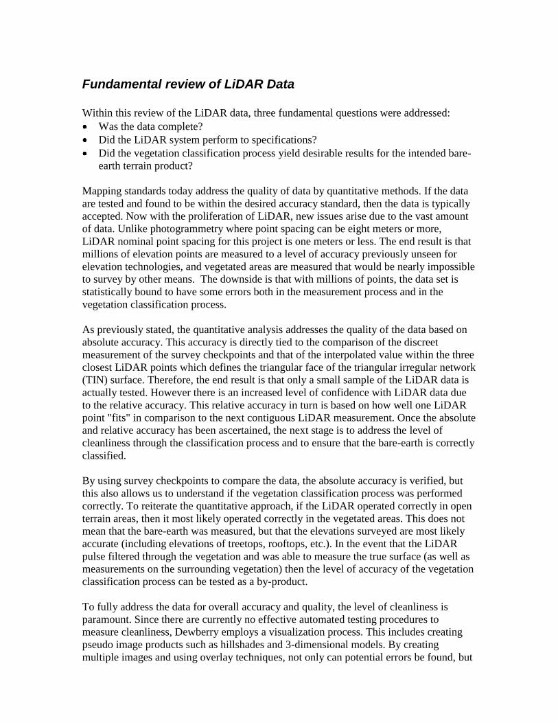
Fundamental review of LiDAR Data
Within this review of the LiDAR data, three fundamental questions were addressed:
Was the data complete?
Did the LiDAR system perform to specifications?
Did the vegetation classification process yield desirable results for the intended bare-
earth terrain product?
Mapping standards today address the quality of data by quantitative methods. If the data
are tested and found to be within the desired accuracy standard, then the data is typically
accepted. Now with the proliferation of LiDAR, new issues arise due to the vast amount
of data. Unlike photogrammetry where point spacing can be eight meters or more,
LiDAR nominal point spacing for this project is one meters or less. The end result is that
millions of elevation points are measured to a level of accuracy previously unseen for
elevation technologies, and vegetated areas are measured that would be nearly impossible
to survey by other means. The downside is that with millions of points, the data set is
statistically bound to have some errors both in the measurement process and in the
vegetation classification process.
As previously stated, the quantitative analysis addresses the quality of the data based on
absolute accuracy. This accuracy is directly tied to the comparison of the discreet
measurement of the survey checkpoints and that of the interpolated value within the three
closest LiDAR points which defines the triangular face of the triangular irregular network
(TIN) surface. Therefore, the end result is that only a small sample of the LiDAR data is
actually tested. However there is an increased level of confidence with LiDAR data due
to the relative accuracy. This relative accuracy in turn is based on how well one LiDAR
point "fits" in comparison to the next contiguous LiDAR measurement. Once the absolute
and relative accuracy has been ascertained, the next stage is to address the level of
cleanliness through the classification process and to ensure that the bare-earth is correctly
classified.
By using survey checkpoints to compare the data, the absolute accuracy is verified, but
this also allows us to understand if the vegetation classification process was performed
correctly. To reiterate the quantitative approach, if the LiDAR operated correctly in open
terrain areas, then it most likely operated correctly in the vegetated areas. This does not
mean that the bare-earth was measured, but that the elevations surveyed are most likely
accurate (including elevations of treetops, rooftops, etc.). In the event that the LiDAR
pulse filtered through the vegetation and was able to measure the true surface (as well as
measurements on the surrounding vegetation) then the level of accuracy of the vegetation
classification process can be tested as a by-product.
To fully address the data for overall accuracy and quality, the level of cleanliness is
paramount. Since there are currently no effective automated testing procedures to
measure cleanliness, Dewberry employs a visualization process. This includes creating
pseudo image products such as hillshades and 3-dimensional models. By creating
multiple images and using overlay techniques, not only can potential errors be found, but

we can also find where the data meets and exceeds expectations. This report will present
representative examples where the LiDAR and post processing had issues but for the
most part the data is of excellent quality.
Prior to the quantitative and qualitative review a series of quality control checks were
performed. This process statistically reviews 100% of the data. This was followed by
reviewing approximately 33% of the tiles at a macro high level and 20% of the tiles in
detail. Our effort concentrated on the coastlines to ensure homogenous data in these
critical areas, but tiles were also selected dispersed throughout the county. The tiles were
selected based on a semi-random approach to ensure a good distribution but tiles were
also selected by land cover type and edge matching with adjacent tiles.
Statistical Review
The project area is approximately 1,072 square miles and is subdivided based on the New
York State Digital Orthoimagery Program stateplane photo tile index
(http://www.nysgis.state.ny.us/gateway/orthoprogram/lot4/suffolk.htm). In total 5,664
tiles were delivered in LAS format. A statistical review of the data was performed to
verify factors such as the number of points per tile, the minimum and maximum Z-values
(as well as other statistics), geographic extents of each tile, and the proper name for each
tile.
To ensure each tile was complete with data, the number of records for each tile was
calculated. This process reviewed if the number of records within each tile was within an
anticipated range. It is expected that some tiles over open bodies of water and on the edge
of the project boundary would have “less” number of records. This review did not find
any tiles that were missing data. See Figure 1
Figure 1 - Number of records in LAS files located by tiles.

To first identify incorrect elevations, the z-minimum and z-maximum values were
reviewed. Some anomalies were identified but all values were properly classified as
“unclassified – Class 1” as per ASPRS LAS standards and the requirements of the scope
of work for this acquisition and processing. Figure 2 illustrates the z minimum value for
each tile. Thirty files have a z minimum under -30ft, all of them in the north east region.
They are mainly situated on the coast and are all over the water. This phenomena can be
seen in Figure 3 and in tiles 14730324 and 14670318 (as well as others). A few files
contain only 1 point in error such as tile 14370272 which contains one point at -55ft on
vegetation and in tile 12840218 with a point at -97ft on a roof but again is “unclassified”.
An examination of the z maximum value indicated 3 files with values around 4000ft but
again these were typically over water and classified correctly (e.g. Figure 4). None of
these erroneous elevations were in the ground (class 2) classification.
Figure 2 – Minimum elevation in each LAS file
Figure 3 – Low elevations located in the water. These are correctly classified.

Figure 4 – Spikes on water with elevations of over 4000 feet (tile 12240198). These points are
properly classified.
The geographic extent of the LAS files were compared to the extent of each tile in the tile
scheme. This ensures that each tile is geographically correct, and that the tile contains the
data within the project boundaries. Figure 9 illustrates that a majority of files has an
extent similar to the tile schema. A few files with too small extent can be found (3 under
50% of tile area, 10 between 50% and 90%) but, once again, they are all in open water
areas. The final process is to compare the geographic extents against the tile name since
the tile name contains the coordinate of the bottom left coordinate. No issues were
identified.
Figure 5 – Comparison between the LiDAR file extent and the tile extent

Quantitative Analysis Checkpoint Survey
The vertical accuracy of the LiDAR data (ground truthing) was performed by surveying
in strategic locations. These checkpoint surveys followed the locational criteria as set
forth by the FEMA Guidelines and Specifications for Flood Hazard Mapping Partners
(Section A.6.4 of Appendix A). The guidelines state: “The assigned Mapping Partner
shall separately evaluate and report on the TIN accuracy… for the main categories of
ground cover in the study area”. It was determined that four land cover were
representative:
1. Open bare-earth terrain – sand, dirt, rock, short grass (less than 0.5 feet)
2. Weeds and Crop – tall grass, crops, small bushes (between 1 ft – 5 ft)
3. Forested areas – deciduous trees (greater than 5 ft)
4. Urban – paved streets, parking lots, areas of buildings.
For consistency with FEMA guidelines, a total of 80 checkpoints were surveyed (see
Figure 6). FEMA requires 20 checkpoints for each of the major land cover category
whereas paragraph 3.2.2 of the National Standard for Spatial Data Accuracy (NSSDA)
states: A minimum of 20 check points shall be tested, distributed to reflect geographic
areas of interest and the distribution of error in the dataset. When 20 points are tested, the
95% confidence level allows one point to fail the threshold given in product
specifications.”
Figure 6 - Survey checkpoint locations and land cover types.

Vertical Accuracy Assessment Using the RMSE Methodology
The first method of testing vertical accuracy is to use the Root Mean Square Error
(RMSE) which is valid when errors follow a normal distribution. This methodology
measures the square root of the average of the set of squared differences between dataset
coordinate values and coordinate values from an independent source of higher accuracy
for identical points. The vertical accuracy assessment compares the measured survey
checkpoint elevations with those of the TIN as generated from the bare-earth LiDAR.
The survey checkpoint‟s X/Y location is overlaid on the TIN and the interpolated Z value
is recorded. This interpolated Z value is then compared to the survey checkpoint Z value
and this difference represents the amount of error between the measurements. The
following tables and graphs outline the vertical accuracy and the statistics of the
associated errors.
95 % of
Totals
RMSE
(ft) Spec=0.61ft
Mean
(ft)
Median
(ft) Skew
Std
Dev
(ft)
# of
Points
Min
(ft)
Max
(ft)
Consolidated 0.27 0.08 0.02 0.75 0.26 76 -0.40 0.86
Open Terrain 0.22 0.09 0.08 1.05 0.21 20 -0.16 0.64
Weeds/Crop 0.28 0.11 0.03 0.60 0.27 20 -0.25 0.66
Forest 0.24 0.07 0.05 -0.19 0.24 18 -0.40 0.39
Urban 0.31 0.04 -0.05 1.37 0.32 18 -0.36 0.86
Table 1 – RMSE and descriptive statistics on 95% of the check points.
LiDAR minus QAQC Checkpoints by Land Cover Type (Best 95%)
-0.6
-0.4
-0.2
0.0
0.2
0.4
0.6
0.8
1.0
1 2 3 4 5 6 7 8 9 10 11 12 13 14 15 16 17 18 19 20
Sorted Data Checkpoints
Fe
et
Open Terrain
Weeds/Crop
Forest
Urban
Figure 7 - Elevation differences between the surveyed QAQC checkpoints and the interpolated
LiDAR with 5% of the outliers removed per FEMA guidelines.

For comparative purposes the Table 2 illustrates the statistics for 100% of the survey
checkpoints. Even with all data the accuracy exceeds the required 0.61 RMSE for the best
95% of points.
100 % of
Totals
RMSE
(ft) Spec=0.61ft
Mean
(ft)
Median
(ft) Skew
Std
Dev
(ft)
# of
Points
Min
(ft)
Max
(ft)
Consolidated 0.36 0.11 0.03 1.16 0.35 80 -0.87 1.52
Open Terrain 0.22 0.09 0.08 1.05 0.21 20 -0.16 0.64
Weeds/Crop 0.28 0.11 0.03 0.60 0.27 20 -0.25 0.66
Forest 0.47 0.19 0.08 1.73 0.44 20 -0.40 1.52
Urban 0.41 0.04 -0.05 0.45 0.42 20 -0.87 0.90
Table 2 - RMSE and descriptive statistics for 100% of checkpoints (80).
Vertical Accuracy Assessment Using the NDEP Methodology
The FEMA methodology above assumes that the data follows a normal distribution and
experience has shown that this is not always the case particularly for vegetated areas. For
comparative purposes the following NDEP method statistics are illustrated.
Land Cover
Category # of Points
FVA ―
Fundamental
Vertical Accuracy
(RMSEz x 1.9600)
Spec=1.19 ft
CVA ―
Consolidated
Vertical Accuracy
(95th Percentile)
Spec=1.19ft
SVA ―
Supplemental
Vertical Accuracy
(95th Percentile)
Target=1.19 ft
Consolidated 80 0.865
Open Terrain 20 0.440 0.412
Weeds/Crop 20 0.536
Forest 20 1.094
Urban 20 0.876
Table 3 – Accuracy for FVA standard
The Fundamental Vertical Accuracy (FVA) at the 95% confidence level equals 1.96
times the RMSE in open terrain only: in open terrain there is no valid excuse why errors
should not follow a normal error distribution, for which the RMSE methodology is
appropriate. Supplemental Vertical Accuracy (SVA) at the 95% confidence level utilizes
the 95th
percentile error individually for each of the other land cover categories, which
may have valid reasons (e.g. problems with vegetation classification) why errors do not
follow a normal distribution (see Figure 8). Similarly the Consolidated Vertical Accuracy
(CVA) at the 95% confidence level utilizes the 95th
percentile error for all land cover
categories combined. This NDEP methodology is used on all 100% of the checkpoints.

Only 4 points are larger than the 95th
percentile but only one point exceeds the
specification. The four points are: PID Land Cover Type Difference
U008 Urban -0.87
U016 Urban 0.90
1014 Forest 1.07
1017 Forest 1.52
Table 4 - Checkpoints greater than the 95th percentile. Note only one point exceeds the criteria of
1.19 ft.
95th Percentile by Land Cover Type
Open Terrain
Weeds/Crop
Forest
Urban
0.00
0.20
0.40
0.60
0.80
1.00
1.20
Land Cover
Fe
et
95th Percentile SVA Target
Figure 8 - 95th Percentile by Land Cover Type
The target objective for this project was to achieve bare-earth elevation data with an
accuracy equivalent to 2 ft contours, which equates to an RMSE of 0.61 ft when errors
follow a normal distribution. With these criteria, the Fundamental Vertical Accuracy of
1.19 ft must be met. Furthermore, it is desired that the consolidated Vertical Accuracy
and each of the Supplemental Vertical Accuracy also meet the 1.19 ft criteria to ensure
that elevations are also accurate in vegetated areas. As summarized in table 3, this data:
Does satisfy the NDEP‟s mandatory Fundamental Vertical Accuracy criteria for 2
ft contours.
Does satisfy the NDEP‟s mandatory Supplemental Vertical Accuracy criteria for
2 ft contours.
Does satisfy the NDEP‟s mandatory Consolidated Vertical Accuracy criteria for 2
ft contours.

Vertical Accuracy Conclusion
Utilizing both methods of vertical accuracy testing, this data meets and exceeds all
specifications. The RMSE of 0.27 ft is less than the FEMA requirement of 0.61 ft and
even using 100% of points the RMSE is 0.36. This data is of excellent quality and should
satisfy most users for high accuracy digital terrain models.

Qualitative Review
Based on the data tested by Dewberry, it is our professional judgment that this data can
easily meet the desired accuracy for not only 2 ft contours, but also will be suitable for
most topographic applications requiring high accuracy. No major issues were
encountered and only a few minor issues were identified. Overall the data was consistent
and no one area was weaker than any other. While assessing this dataset, one of our
focuses was to review the data as a whole and look for significant anomalies and not
micro issues such as one or two erroneous classed points. It is assumed that data collected
on a volume of this scale may have unidentified errors at the local level, and may require
slight modifications to fit specific application needs. For example, transportation groups
may need the bridge deck elevations whereas the hydrologist would prefer the bridges
removed. Overall this data will meet the needs of the general users of elevations data and
is excellent for floodplain and coastal mapping.
Contractually our QAQC process was to review 20% of the data. However, we reviewed
34% of the data on a generalized level and 20% at a detailed level due to increased
productivity processes. This approach allowed us to perform analysis where it was
required, and where anomalies had been identified. The generalized level reviewed the
data at a scale of 1:4,000. If an area looked to have issues it was further reviewed using a
multitude of techniques developed by Dewberry which includes looking at point clouds,
surfaces, TINs, hillshades, intensity images and ortho photos if required. Figure 9
illustrates the tiles that were qualitatively reviewed.
To reiterate, the data for the most part is excellent and meets all the desired and required
specifications. It exhibits excellent accuracy and superior vegetation classification,
providing a quality bare-earth data product. The issues identified below are extremely
minor and have minimal impact on the data and the ability to use this topographic data.
One issue that should be noted is that the contract for acquisition and processing,
identified two classes of either: Class “1” for unclassified and Class “2” for ground.
There is no distinction for water and therefore some water points may be classified as
ground since their elevations are equal to the surrounding ground points. The mandate of
the contract has been fulfilled but further processing may be required for specific
applications.

Figure 9 - Tiles evaluated for the qualitative analysis
One minor issue for the bare-earth terrain is the classification around bridges. As
previously stated, some users may require bridges be removed (classified to non-ground)
while others may require them classified as ground. For this dataset most of the bridges
have been retained. However Figure 10 illustrates where the outer portions of the bridge
have been removed, but the central structure still exists. For the user community if this is
an issue this is easily remedied since it is clearly identifiable and the data can be
reclassified. Figure 11 illustrates where a bridge has been completely removed which is
inconsistent with the other bridges. Figure 12 illustrates that the bridge has been retained
but that there are “ground” elevations west of the bridge as they LiDAR vendor was not
contracted to identify water as a separate classification.
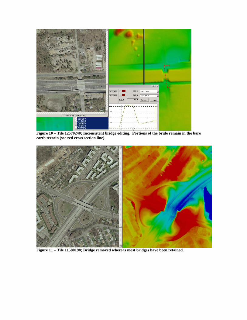
Figure 10 – Tile 12570240; Inconsistent bridge editing. Portions of the bride remain in the bare
earth terrain (see red cross section line).
Figure 11 – Tile 11580198; Bridge removed whereas most bridges have been retained.

Figure 12 – Tile 14400340; Bridge is retained but some water elevations are classified as “ground”
(left side of bridge). This is within scope but users should be aware that not all elevations are
specifically the ground.
Typical of most LiDAR sensors, anomalies of sporadic low points termed „divots” can be
found intermittently throughout the project. Although it is a fairly common occurrence
most of the elevations are incorrect for only one point which causes the depressions.
Figure 13 illustrates one point located in the middle of the road that is over 7 ft deep
which we can assume is not correct. Although this data does contain potential divots,
there are very few to warrant reprocessing.

Figure 13 – Tile 1155202; Divot located in middle of road (see red cross section line).
Due to the vast amounts of data and geographic phenomena, the classification algorithms
can sometimes erroneously classify data. This misclassification results in artifacts which
can be remnants of vegetation or manmade structures that do not represent the bare-earth
terrain. Figure 14 - Figure 18 illustrates potential artifacts based on the visual inspections
of the bare-earth terrain. None of these tiles have been ground truthed and therefore are
identified only as potential issues. It is evident that these potential areas are relatively
small and easily within the specification of being 95% cleaned of artifacts.
Figure 14 – Tile 11340236; potential artifacts.

Figure 15 – Tile 11490230; potential artifacts (white arrows).
Figure 16 – Tile 13680302 potential artifacts (white arrows)

Figure 17 – Tile 13680302 Intensity image for comparative purposes. The potential artifacts appear
to be part of the same forested area and next to a small clearing (white arrows).
Figure 18 – Tile 14580278; Potential artifacts however the ortho photo identifies fairly large
structures that have been misclassified.
An additional phenomenon with LiDAR is the “corn row” effect. There are multiple
reasons as to why this happens but the end result is that adjacent scan lines are slightly
offset from each other. This will give the effect that there are alternating rows of higher
and then lower elevations. Although this is common with LiDAR data, as long as the
elevation differences are a less than 20 cm and that the occurrences are minimized, it is
typically acceptable since it is within the noise and accuracy levels. However this also

can be an indication that the sensor is mis-calibrated, or offsets exist between adjacent
flight lines so each area identified is analyzed. Our review did not find significant corn
row affects and all elevations were within acceptable limits. Figure 20 illustrates a slight
offset between two scan lines. Again this is within acceptable levels. Figure 21 and
Figure 22 illustrate a slight offset between three adjacent scans. The data for this project
was collected with a side lap of 100% so in essence all areas have a minimum of 2 flight
scans over the same area. However in this figure there is a portion of an area (scan line 3)
where it is only covered by one scan line. Since it only has one scan, the data appears
smooth. Outside of this area scan line 3 overlaps with scan line 1 and scan line 2 where
there is this slight elevation discrepancy which causes the corn row affect. Again this
offset is well within tolerances of less that 15 cm.
Figure 19 - Tile 1362030 with corn row affect. This is within acceptable limits as it is less than 15 cm.

Figure 20 - Tile 14910316 illustrates a slight offset between scan lines. This is within acceptable limits
as it is approximately 15cm.
Figure 21 - Tile 14700204 bare-earth terrain overlaid with the points. Three scan lines are apparent
which can be seen by the different scan line pattern.

Figure 22 - Tile 14700204 corn row affect and different levels of smoothness between the three scan
lines.
Figure 23 - Excellent example of the bare-earth terrain definition for a group of tiles. This is a good
representation of the quality of the data.

Conclusion
Overall the data exhibited excellent detail in both the absolute and relative accuracy. The
level of cleanliness for a bare-earth terrain is of the highest quality and no major
anomalies were found. The figures highlighted above are a sample of the minor issues
that were encountered and are not representative of the vast majority of the data which is
of excellent quality data. This data will meet the needs of FEMA, FEMA contractors for
coastal and flood mapping, and most of the user community.

Appendix A
Ground Truth Survey Values
PID E N Elevation zLidar Land Cover Type DeltaZ
G007 1480327.74 315450.61 1.03 0.87 Open Terrain -0.16
G006 1447745.84 359945.17 6.72 6.58 Open Terrain -0.14
G020 1195660.74 244034.43 46.80 46.71 Open Terrain -0.09
G002 1369033.63 290331.75 42.49 42.40 Open Terrain -0.08
G017 1148901.98 217051.44 103.54 103.46 Open Terrain -0.08
G008 1313306.88 286870.59 103.57 103.50 Open Terrain -0.07
G005 1328161.84 235843.61 18.89 18.83 Open Terrain -0.06
G010 1240501.79 204600.45 6.15 6.10 Open Terrain -0.06
G004 1329183.78 230744.30 3.63 3.62 Open Terrain -0.01
G011 1572764.31 336498.56 88.43 88.50 Open Terrain 0.07
G009 1233467.48 226757.10 74.58 74.66 Open Terrain 0.08
G016 1157211.14 209897.88 63.45 63.56 Open Terrain 0.11
G003 1471413.95 290768.83 18.55 18.66 Open Terrain 0.11
G019 1166298.51 190379.16 6.28 6.42 Open Terrain 0.14
G012 1569358.41 335268.87 52.21 52.40 Open Terrain 0.19
G013 1548862.72 328027.63 6.65 6.89 Open Terrain 0.24
G001 1374714.61 296759.22 53.88 54.13 Open Terrain 0.25
G015 1160496.05 278373.29 6.90 7.29 Open Terrain 0.39
G018 1160863.85 183926.04 4.33 4.73 Open Terrain 0.40
G014 1243527.77 286868.75 205.63 206.26 Open Terrain 0.64
W019 1196386.22 247847.42 73.98 73.73 Weeds/Crop -0.25
W002 1374884.1 287777.55 14.75 14.50 Weeds/Crop -0.25
W001 1377268.25 289280.65 22.91 22.67 Weeds/Crop -0.24
W009 1482207.63 320196.85 7.55 7.41 Weeds/Crop -0.14
W011 1229906.3 229568.39 89.76 89.66 Weeds/Crop -0.10
W003 1469727.3 293381.49 29.09 29.02 Weeds/Crop -0.06
W006 1450648.38 360367.90 21.24 21.21 Weeds/Crop -0.03
W007 1454147.88 360123.06 15.65 15.64 Weeds/Crop -0.01
W004 1466690.36 295282.65 42.83 42.85 Weeds/Crop 0.02
W005 1331201.48 230188.38 7.01 7.03 Weeds/Crop 0.03
W020 1310595.22 256650.78 42.41 42.45 Weeds/Crop 0.04
W008 1478982.32 320834.44 6.56 6.64 Weeds/Crop 0.08
W012 1574182.64 335228.51 60.31 60.46 Weeds/Crop 0.15
W015 1164823.28 276838.43 12.99 13.15 Weeds/Crop 0.17
W018 1166874.86 188730.21 6.20 6.45 Weeds/Crop 0.25
W017 1164175.34 183645.04 5.23 5.53 Weeds/Crop 0.31
W014 1156237.62 282196.71 10.90 11.35 Weeds/Crop 0.44
W016 1160624.79 278590.62 10.80 11.32 Weeds/Crop 0.52
W010 1312674.41 284405.93 99.56 100.09 Weeds/Crop 0.53
W013 1547794.86 327804.46 4.79 5.45 Weeds/Crop 0.66
1005 1478080.57 319601.58 27.07 26.66 Forest -0.40

1008 1464590.65 298012.04 115.65 115.41 Forest -0.24
1009 1311179.75 286381.86 82.78 82.61 Forest -0.17
1002 1441974.77 356452.24 26.97 26.84 Forest -0.13
1015 1154585.95 214359.54 84.29 84.21 Forest -0.08
1003 1376250.39 293132.18 34.66 34.60 Forest -0.06
1019 1197638.41 241792.98 50.01 49.96 Forest -0.04
1000 1454700.73 358474.11 7.18 7.17 Forest -0.01
1021 1198986.81 247652.23 70.74 70.79 Forest 0.05
1013 1326918.13 236807.23 33.48 33.53 Forest 0.06
1011 1240970.46 224482.92 63.96 64.05 Forest 0.09
1006 1468614.43 294373.45 40.19 40.42 Forest 0.23
1012 1571192.6 333756.51 79.75 79.99 Forest 0.24
1016 1166566.51 190298.56 8.18 8.42 Forest 0.24
1018 1168268.15 190875.32 6.54 6.91 Forest 0.36
1010 1235387.36 222348.74 56.83 57.21 Forest 0.37
1004 1377549.68 283038.83 7.50 7.89 Forest 0.38
1020 1199392.8 236984.98 76.16 76.56 Forest 0.39
1014 1240819.28 284545.04 17.32 18.39 Forest 1.07
1017 1173958.56 194041.63 5.61 7.13 Forest 1.52
U008 1241762.81 222406.96 59.40 58.52 Urban -0.87
U005 1481639.82 320274.04 10.77 10.41 Urban -0.36
U019 1145983.26 208936.59 74.15 73.88 Urban -0.27
U009 1232621.9 234659.93 100.69 100.46 Urban -0.22
U018 1152933.9 207285.11 65.95 65.76 Urban -0.20
U012 1569081.15 334549.23 47.88 47.76 Urban -0.12
U006 1315019.3 292843.92 84.66 84.55 Urban -0.11
U004 1445092.47 356048.00 5.51 5.40 Urban -0.11
U007 1308531.08 286174.64 110.48 110.38 Urban -0.10
U001 1370605.2 288024.18 22.56 22.51 Urban -0.05
U014 1554532.35 328192.03 44.98 44.94 Urban -0.04
U013 1551312.23 323340.71 15.33 15.30 Urban -0.02
U002 1466802.37 292223.36 45.38 45.37 Urban -0.01
U003 1326425.58 233993.94 24.29 24.35 Urban 0.06
U020 1170724.49 195850.43 8.84 8.92 Urban 0.09
U010 1239203.37 209656.82 13.68 13.97 Urban 0.29
U017 1163397.21 274684.67 7.83 8.33 Urban 0.50
U011 1235644.81 206414.83 10.06 10.62 Urban 0.56
U015 1241371.25 285838.32 6.72 7.58 Urban 0.86
U016 1237832.98 287802.94 6.25 7.15 Urban 0.90