2002 IEEE TRANSACTIONS ON CONTROL SYSTEMS …

2002 IEEE TRANSACTIONS ON CONTROL SYSTEMS TECHNOLOGY, VOL. 24, NO. 6, NOVEMBER 2016

Predictor Observers for Proportional NavigationSystems Subjected to Seeker Delay

John Holloway and Miroslav Krstic, Fellow, IEEE

Abstract— We propose predictor observers as viable toolsto compensate for pure time delays in the seeker subsystemof missile guidance systems employing proportional navigationguidance (PNG). With the intention of use in terminal guidancein which the missile is already on a near-collision course witha target, we demonstrate that a classical predictor observerfor linear time-delay systems is input-to-state stable (ISS) withrespect to bounded target maneuver and measurement distur-bances. We then show how the classical predictor observer can beimplemented as a Kalman filter for the delayed state augmentedwith a predictor. Finally, we illustrate the practicality of theapproach in missile guidance system design through two examplesthat exhibit seeker delay and random target maneuvers. For bothexamples, numerical simulations show that predictor observerguidance laws are able to substantially reduce miss distanceversus baseline PNG laws that have no delay compensation,inviting further studies of the approach for designing real missileguidance systems in practice.

Index Terms— Delay, guidance, missile, observer, predictor,stability.

I. INTRODUCTION

TACTICAL missile guidance laws exhibit performancedegradation when lags and delays in the homing loop

are taken into account [1]–[6]. Depending on the missileconsidered, significant lags or delays can exist in the flightcontrol system, the seeker and filter dynamics, the digitalprocessing of the guidance and control algorithms, or anycombination of these. The effects of these systems com-bined are sometimes called guidance system dynamics inthe literature, and [1]–[3] provide a good introduction tothe adverse effects they have on guidance law performance.Lags and delays in the homing loop become more detrimen-tal when coupled with target maneuvering during terminalguidance, in which they become significant fractions of thetime-to-go (tgo) [1], [2], [7].

A common approach used to mitigate guidance sys-tem dynamics is to model them as a first-order lag orseries of lags as part of the dynamic system to becontrolled [1]–[5], [7]–[9]. This approach is adequate for manypurposes, but in some situations, it may be more appropriateto model some homing loop dynamics as a pure time delay

Manuscript received March 23, 2015; revised October 31, 2015; acceptedJanuary 6, 2016. Date of publication February 26, 2016; date of currentversion October 14, 2016. Manuscript received in final form February 2, 2016.Recommended by Associate Editor S. Tarbouriech. (Corresponding author:John Holloway.)

The authors are with the Department of Mechanical and Aerospace Engi-neering, University of California at San Diego, La Jolla, CA 92093 USA(e-mail: [email protected]; [email protected]).

Digital Object Identifier 10.1109/TCST.2016.2526666

rather than a lag. For example, seeking a simplified modelof the target maneuver estimation process and understandingthat estimates of target acceleration converge more slowly thanestimates of target position, Shinar et al. [4], [5] modeled hom-ing loop filter dynamics as a pure delay in the estimate of targetacceleration. The pure delay model of filter dynamics wasalso employed in [6], [8], and [10]–[13]. On the other hand,Gurfil [10], [11], Hablani [14], Xu et al. [15], Lum et al. [16],and Dhananjay et al. [17] modeled pure delays in the seekerdynamics on the basis that some optical passive seekers canexhibit a significant delay in providing line-of-sight (LOS) ratemeasurements to the guidance law.

There exist relatively few published studies specificallyaimed at mitigating performance degradation due to a puretime delay in the seeker measurement. Hablani [14] intro-duced a velocity feed-forward approach to compensate forpassive seeker delays in terminal guidance of exoatmosphericinterceptors and showed that the technique can be effective inreducing miss distance when various process noise covariancematrices are used. Xu et al. [15] demonstrated two methodsfor estimating the minimum achievable miss distance forproportional navigation guidance (PNG) with delayed LOSrate measurement, assuming an estimated bound on the error inthe LOS rate estimate. Lum et al. [16] proposed a sliding modeguidance law assuming delayed LOS rate measurement and asimple estimator for LOS rate and showed that it may achievea lower miss distance than PNG, depending on guidanceparameters and initial conditions. And then most recently,Dhananjay et al. [17] formulated a PNG problem havingdelayed LOS rate measurement as a Lyapunov–Krasovskiistability analysis using a delay differential equation for thedelayed LOS rate and determined the effective navigationratio (N ′) and time-to-go (tgo) required to guarantee decreasingbehavior of the Lyapunov function used to characterize thestability of the LOS rate. We note that all of these solutionsdepend strongly on the target engagement model assumed,but this is also true of missile guidance system design ingeneral.

As far as we know, the delay compensation techniquesknown as predictor feedback have not yet been applied totactical missile guidance problems. Tracing their origins backto the Smith predictor in 1959, the ideas of predictor feedbackhave been applied to time-delay systems for decades, withrecent advances extending to nonlinear systems [18], [19],nonconstant delays [19], and the applications of these tech-niques [20]. As the first step in studying the applicationof predictor feedback to missile guidance laws subjected to

1063-6536 © 2016 IEEE. Personal use is permitted, but republication/redistribution requires IEEE permission.See http://www.ieee.org/publications_standards/publications/rights/index.html for more information.

HOLLOWAY AND KRSTIC: PREDICTOR OBSERVERS FOR PROPORTIONAL NAVIGATION SYSTEMS SUBJECTED TO SEEKER DELAY 2003

time delays, we recently discovered in [21] that a classical pre-dictor observer for linear time-delay systems [18], [22], [23]could be useful for missile guidance laws subjected to seekerdelay in the near-collision course. For practical motivation,we note that in the design of real weapon systems, perfor-mance is often constrained by the monetary cost required toimplement the design. Dhananjay et al. [17] proposed that theoverall cost of a missile guidance system could be lowered byleveraging low-cost optical seekers, which exhibit significantcomputational delays, and combining them with improvedguidance algorithms that compensate for the delays. We seekto contribute to this effort by demonstrating that the classicalpredictor observer for linear systems can be used to improvethe performance of a widely used guidance law subjected toa pure time delay in the seeker measurement. Because of itsfamiliarity, simplicity, and long history of performance in realmissile guidance systems, we selected a form of PNG as ourbaseline guidance law for this study.

The remainder of this paper proceeds as follows. Section IIpresents our missile–target engagement model. Section IIIintroduces PNG as the baseline guidance law for our analysis.Section IV presents the predictor observer state estimatorwe use and demonstrates its stability with respect to targetmaneuver and disturbances and time delay in the seekermeasurement. Section V illustrates how the approach couldaid in the design of real missile guidance systems throughtwo examples. Section VI summarizes the main contributionsof this paper.

II. MISSILE–TARGET ENGAGEMENT MODEL

In this paper, we focus on terminal missile guidance inwhich the missile has already achieved a near-collision coursewith a target. In the near-collision course, the missile-to-targetLOS angle and the LOS rate have already been made small,and the nonlinear guidance kinematics are adequately modeledby linear perturbational equations. We invoke the followingassumptions to obtain our model.

1) A1 (Planar Engagement): The missile–target engage-ment is confined to a 2-D plane.

2) A2 (Tail Chase): The flight path angles of the missileand the target are approximately equal, and the missilepursues the target from behind.

3) A3 (Constant Velocity): The total missile velocity VM

and total target velocity VT are approximately constant,and VM > VT .

4) A4 (Small Angles): The missile-to-target LOS angleremains small relative to its initial value.

5) A5 (Missile Forces): Gravitational, aerodynamic, andlongitudinal propulsive forces affecting the missile aresmall relative to the missile divert forces resulting fromguidance.

6) A6 (Axis Decoupling): The missile employs roll controlsuch that the effects of missile axis coupling can beneglected.

7) A7 (Flight Control): The missile flight control dynam-ics are fast enough such that their effects can beneglected.

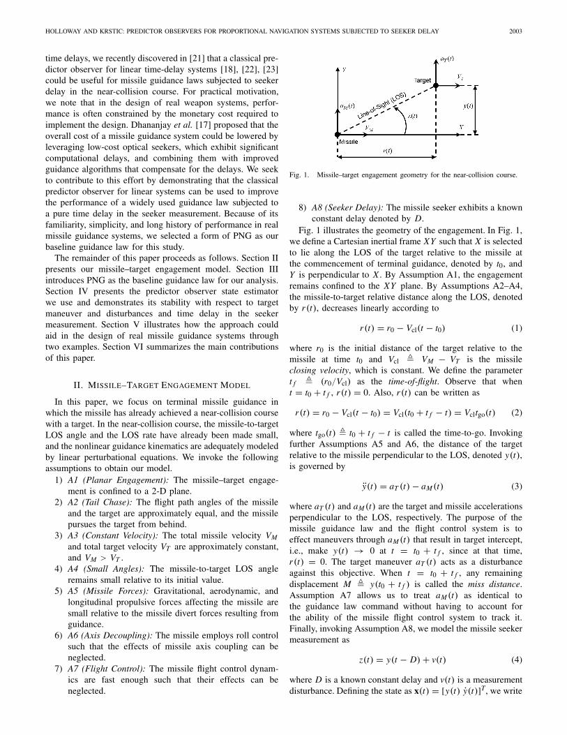
Fig. 1. Missile–target engagement geometry for the near-collision course.

8) A8 (Seeker Delay): The missile seeker exhibits a knownconstant delay denoted by D.

Fig. 1 illustrates the geometry of the engagement. In Fig. 1,we define a Cartesian inertial frame XY such that X is selectedto lie along the LOS of the target relative to the missile atthe commencement of terminal guidance, denoted by t0, andY is perpendicular to X . By Assumption A1, the engagementremains confined to the XY plane. By Assumptions A2–A4,the missile-to-target relative distance along the LOS, denotedby r(t), decreases linearly according to

r(t) = r0 − Vcl(t − t0) (1)

where r0 is the initial distance of the target relative to themissile at time t0 and Vcl � VM − VT is the missileclosing velocity, which is constant. We define the parametert f � (r0/Vcl) as the time-of-flight. Observe that whent = t0 + t f , r(t) = 0. Also, r(t) can be written as

r(t) = r0 − Vcl(t − t0) = Vcl(t0 + t f − t) = Vcltgo(t) (2)

where tgo(t) � t0 + t f − t is called the time-to-go. Invokingfurther Assumptions A5 and A6, the distance of the targetrelative to the missile perpendicular to the LOS, denoted y(t),is governed by

y(t) = aT (t) − aM (t) (3)

where aT (t) and aM (t) are the target and missile accelerationsperpendicular to the LOS, respectively. The purpose of themissile guidance law and the flight control system is toeffect maneuvers through aM (t) that result in target intercept,i.e., make y(t) → 0 at t = t0 + t f , since at that time,r(t) = 0. The target maneuver aT (t) acts as a disturbanceagainst this objective. When t = t0 + t f , any remainingdisplacement M � y(t0 + t f ) is called the miss distance.Assumption A7 allows us to treat aM (t) as identical tothe guidance law command without having to account forthe ability of the missile flight control system to track it.Finally, invoking Assumption A8, we model the missile seekermeasurement as

z(t) = y(t − D) + v(t) (4)

where D is a known constant delay and v(t) is a measurementdisturbance. Defining the state as x(t) = [y(t) y(t)]T, we write


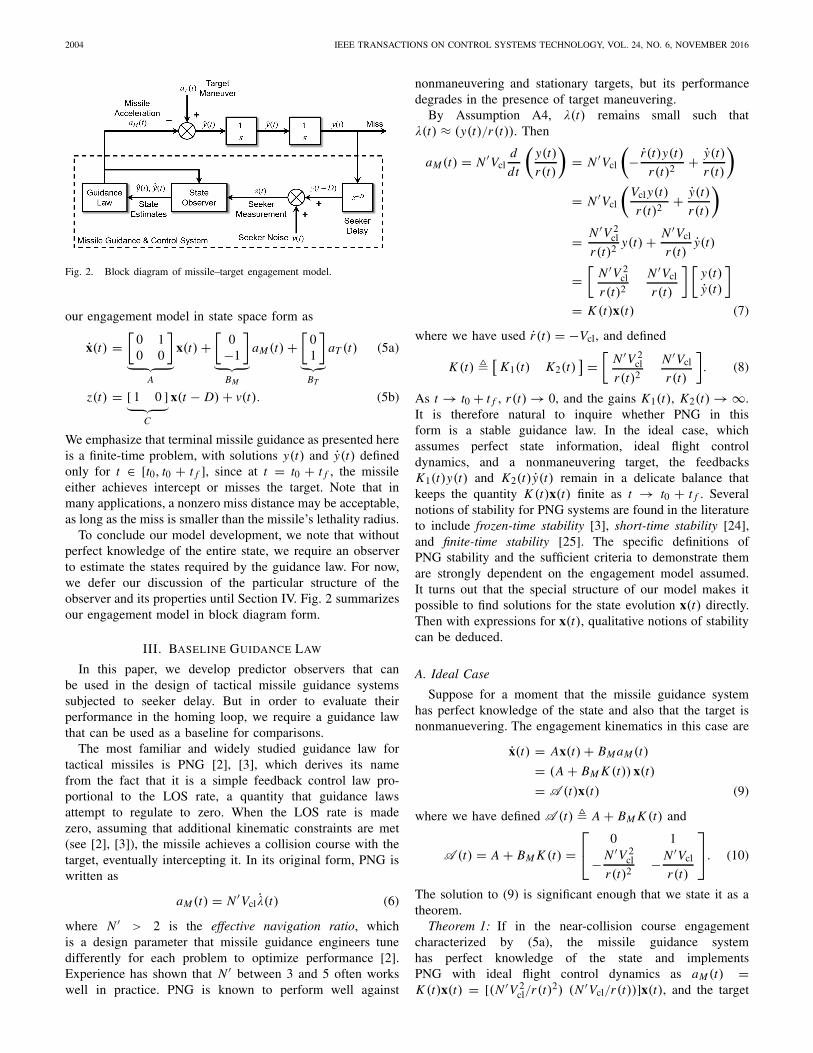
Fig. 2. Block diagram of missile–target engagement model.

our engagement model in state space form as

x(t) =[

0 10 0

]︸︷︷︸

A

x(t) +[

0−1

]︸︷︷︸

BM

aM (t) +[

01

]︸︷︷︸

BT

aT (t) (5a)

z(t) = [ 1 0 ]︸︷︷︸C

x(t − D) + v(t). (5b)

We emphasize that terminal missile guidance as presented hereis a finite-time problem, with solutions y(t) and y(t) definedonly for t ∈ [t0, t0 + t f ], since at t = t0 + t f , the missileeither achieves intercept or misses the target. Note that inmany applications, a nonzero miss distance may be acceptable,as long as the miss is smaller than the missile’s lethality radius.

To conclude our model development, we note that withoutperfect knowledge of the entire state, we require an observerto estimate the states required by the guidance law. For now,we defer our discussion of the particular structure of theobserver and its properties until Section IV. Fig. 2 summarizesour engagement model in block diagram form.

III. BASELINE GUIDANCE LAW

In this paper, we develop predictor observers that canbe used in the design of tactical missile guidance systemssubjected to seeker delay. But in order to evaluate theirperformance in the homing loop, we require a guidance lawthat can be used as a baseline for comparisons.

The most familiar and widely studied guidance law fortactical missiles is PNG [2], [3], which derives its namefrom the fact that it is a simple feedback control law pro-portional to the LOS rate, a quantity that guidance lawsattempt to regulate to zero. When the LOS rate is madezero, assuming that additional kinematic constraints are met(see [2], [3]), the missile achieves a collision course with thetarget, eventually intercepting it. In its original form, PNG iswritten as

aM (t) = N ′Vclλ(t) (6)

where N ′ > 2 is the effective navigation ratio, whichis a design parameter that missile guidance engineers tunedifferently for each problem to optimize performance [2].Experience has shown that N ′ between 3 and 5 often workswell in practice. PNG is known to perform well against

nonmaneuvering and stationary targets, but its performancedegrades in the presence of target maneuvering.

By Assumption A4, λ(t) remains small such thatλ(t) ≈ (y(t)/r(t)). Then

aM (t) = N ′Vcld

dt

(y(t)

r(t)

)= N ′Vcl

(− r(t)y(t)

r(t)2 + y(t)

r(t)

)

= N ′Vcl

(Vcl y(t)

r(t)2 + y(t)

r(t)

)

= N ′V 2cl

r(t)2 y(t) + N ′Vcl

r(t)y(t)

=[

N ′V 2cl

r(t)2

N ′Vcl

r(t)

] [y(t)y(t)

]

= K (t)x(t) (7)

where we have used r(t) = −Vcl, and defined

K (t) �[

K1(t) K2(t)] =

[N ′V 2

cl

r(t)2

N ′Vcl

r(t)

]. (8)

As t → t0 + t f , r(t) → 0, and the gains K1(t), K2(t) → ∞.It is therefore natural to inquire whether PNG in thisform is a stable guidance law. In the ideal case, whichassumes perfect state information, ideal flight controldynamics, and a nonmaneuvering target, the feedbacksK1(t)y(t) and K2(t)y(t) remain in a delicate balance thatkeeps the quantity K (t)x(t) finite as t → t0 + t f . Severalnotions of stability for PNG systems are found in the literatureto include frozen-time stability [3], short-time stability [24],and finite-time stability [25]. The specific definitions ofPNG stability and the sufficient criteria to demonstrate themare strongly dependent on the engagement model assumed.It turns out that the special structure of our model makes itpossible to find solutions for the state evolution x(t) directly.Then with expressions for x(t), qualitative notions of stabilitycan be deduced.

A. Ideal Case

Suppose for a moment that the missile guidance systemhas perfect knowledge of the state and also that the target isnonmanuevering. The engagement kinematics in this case are

x(t) = Ax(t) + BM aM (t)

= (A + BM K (t)) x(t)

= A (t)x(t) (9)

where we have defined A (t) � A + BM K (t) and

A (t) = A + BM K (t) =⎡⎣ 0 1

− N ′V 2cl

r(t)2 − N ′Vcl

r(t)

⎤⎦. (10)

The solution to (9) is significant enough that we state it as atheorem.

Theorem 1: If in the near-collision course engagementcharacterized by (5a), the missile guidance systemhas perfect knowledge of the state and implementsPNG with ideal flight control dynamics as aM (t) =K (t)x(t) = [(N ′V 2

cl/r(t)2) (N ′Vcl/r(t))]x(t), and the target


is nonmaneuvering, then the state x(t) evolves fort ∈ [t0, t0 + t f ] according to

x(t) = 1

1 − N ′ �(t, t0)x(t0) (11)

where �(t, t0) is the state transition matrix, defined as thematrix that satisfies

d

dt�(t, t0) = A (t)�(t, t0) (12a)

�(t0, t0) = (1 − N ′)I (12b)

where N ′ > 2, and

�11(t, t0) = r(t)

r0

[(r(t)

r0

)N ′−1

− N ′]

(13a)

�12(t, t0) = r(t)

Vcl

[(r(t)

r0

)N ′−1

− 1

](13b)

�21(t, t0) = N ′Vcl

r0

[1 −

(r(t)

r0

)N ′−1]

(13c)

�22(t, t0) = 1 − N ′(

r(t)

r0

)N ′−1

. (13d)

Proof: See Appendix A. �An important consequence of Theorem 1 is that with perfect

knowledge of the state, ideal flight control, and a nonmaneu-vering target, PNG in the near-collision course achieves zeromiss distance in finite time.

Corollary 1: If the hypotheses of Theorem 1 are met, thenat t = t0 + t f , y(t0 + t f ) = 0 and y(t0 + t f ) = (N ′Vcl y0/r0) + y0.

Proof: The proof follows by inspection of the solutionof x(t). As t → t0 + t f , r(t) → 0. Then for any integer M ,(r(t)/r0)

M → 0. So as t → t0 + t f , y(t) → 0 and y(t) →(N ′Vcl y0/r0) + y0. �

In other words, in the near-collision course, PNG exhibitsa somewhat peculiar result: the miss distance is regulated tozero, but the rate of the missile perpendicular to the LOS isnot regulated to anything, and ends up converging to somefinite value that depends on N ′, the initial conditions, andthe time-of-flight t f = r0/Vcl. Since even with perfect stateinformation, perfect flight control, and a nonmaneuveringtarget, not all of the state is regulated to x(t) = 0, once werelax one or more of these assumptions, we do not expectthe desirable, traditional stability concepts like input-to-statestability [26], [27] to hold. Despite this inconvenience, we canstill establish a less useful form of stability, but we requireadditional notation. We denote the Euclidean 2-norm of ann-element vector of real elements x by |x| = (xT x)1/2, theinduced 2-norm of an m × n matrix of real elements Aby |A| = [λ(AT A)]1/2, where λ(·) denotes the maximumeigenvalue of a matrix, and the induced ∞-norm of A by|A|∞ = maxi

∑nj=1 |ai j |, where ai j is the element of A in the

i th row and the j th column.Corollary 2: The origin x = 0 of (11) is globally uniformly

stable for t ∈ [t0, t0 + t f ].

Proof: From (11), we have

|x(t)| ≤∣∣∣∣ 1

1 − N ′

∣∣∣∣ |�(t, t0)||x(t0)|

≤√

2

|1 − N ′| |�(t, t0)|∞|x(t0)|. (14)

Using (13), we find that

|�(t, t0)|∞ ≤ max

{N ′

(1

t f+ 1

)− 1, N ′ + t f

}(15)

which is always bounded for finite N ′ and t f . Since|�(t, t0)|∞ is bounded for all t ∈ [t0, t0 + t f ], x(t) remainsbounded, so x = 0 is stable for all t ∈ [t0, t0 + t f ]. Thestability is global, and since (15) is independent of t0, thestability is also uniform. �

B. General Case

For the general case where the state must be estimated usingthe seeker measurement (4), and the target is maneuvering,we define the estimate of the state as x(t) � [y(t) ˆy(t)]T, andassume that r(t) is still known perfectly according to (1). ThePNG law then becomes

aM (t) = K (t)x(t). (16)

Then defining the state estimation error as x(t) � x(t) − x(t),we have

aM (t) = K (t)x(t) − K (t)x(t) (17)

and the engagement kinematics become

x(t) = Ax(t) + BM aM (t) + BT aT (t)

= (A + BM K (t))x(t) − BM K (t)x(t) + BT aT (t)

= A (t)x(t) − BM K (t)x(t) + BT aT (t). (18)

The solution to (18) is another important consequence ofTheorem 1.

Corollary 3: For the near-collision course engagementcharacterized by (5a), in which the missile implementsPNG with ideal flight control in the formaM (t) = K (t)x(t) = [(N ′V 2

cl/r(t)2) (N ′Vcl/r(t))]x(t),where x(t) = [y(t) ˆy(t)]T is the state estimate provided byan observer, and x(t) is the state estimation error, and thestate evolves for t ∈ [t0, t0 + t f ] and N ′ > 2 according to

x(t) = 1

1 − N ′ �(t, t0)x(t0)

− 1

1 − N ′

∫ t

t0�(t, θ)BM K (θ)x(θ)dθ

+ 1

1 − N ′

∫ t

t0�(t, θ)BT aT (θ)dθ. (19)

Proof: The proof follows from (11) and (18) by simpleapplication of the variation of parameter formula. �

Since by (11) not all of the state is regulated to zero evenwithout the disturbances x(t) and aT (t), input-to-state stabilitycannot be established. Furthermore, the finite-time nature ofPNG in the near-collision course makes it difficult to obtainmeaningful bounds on the trajectories x(t) once the distur-bances x(t) and aT (t) are added to the problem. For these


reasons, we consider a rigorous finite-time stability analysisof (19) to be an open problem. Without proven statements onthe stability of (19), as is typically done in practice, we rely onnumerical simulations to verify the stability of our guidancelaws in the closed loop.

IV. PREDICTOR OBSERVERS

Due to the finite-time nature of our terminal guidanceproblem, we require a state observer that not only remainsstable but also provides accurate estimates of the state asquickly as possible. In this section, we show how such anobserver can be designed by leveraging a classical predictorobserver for linear time-delay systems.

A. Classical Predictor Observer

For the linear time-invariant system

x(t) = Fx(t) + G1u(t) + G2w(t) (20)

z(t) = H x(t − D) + G3v(t) (21)

with control input u(t), bounded disturbances w(t) and v(t),and D > 0 a constant measurement delay, the state x(t) canbe estimated using the classical predictor observer for lineartime-delay systems [18], [22], [23]

x(t) = eF D�(t) +∫ t

t−DeF(t−τ )G1u(τ )dτ (22)

�(t) = F�(t) + G1u(t − D) + L[z(t) − H�(t)] (23)

where x(t) is the state estimate, �(t) is an estimate of thedelayed state x(t − D), and L is chosen such that (F − L H) isHurwitz. Note that for w(t) = 0 and v(t) = 0, (23) is simply aLuenberger observer for the delayed state, x(t − D); thus, with(F − L H ) Hurwitz, it provides an exponentially convergentestimate of x(t − D). Then the estimate for the current stateis arrived at (22) by application of the variation of parameterformula. We call (22) the predictor and (23) the observer.Thus, with (22) and (23) combined, we have a predictorobserver for the current state, x(t), given a measurement ofthe delayed state characterized by (21).

There exist other observers that could be used for ourengagement model with seeker delay, such as the cascadeobservers introduced in [28] and later used with sliding modecontrol in [29]. However, while those observers may appearto be simpler since they do not involve a distributed delay, theobservers have a higher dynamical order, since they estimatethe state at a number of delayed states instead of a singledelayed state. For this reason, classical predictor observer (22),(23) may be easier to implement in missile guidance systemdesign.

Predictor observer (22), (23) for w = 0 and v = 0 wasshown to be exponentially stable in [18]. In the following,we show that for w = 0 and v = 0, this predictor observer isalso input-to-state stable (ISS) [26], [27]. For easy reference,we state the definition of input-to-state stability, in which theusual definitions of class K and class K L functions [26]are implied.

Definition 1 (Input-to-State Stability): The system is saidto be ISS if there exist a class K L function β and class

K functions γ j such that for any initial state x(t0) and anybounded inputs u j (t), for j = 1, 2, . . . , n, the solution x(t)exists for all t ≥ t0 and satisfies

|x(t)| ≤ β(|x(t0)|, t − t0) +n∑

j=1

γ j

(sup

t0≤τ≤t|u j (τ )|

). (24)

We now state the main result of this work.Theorem 2: For system (20), (21) with control input u,

a known, constant measurement delay D, and bounded distur-bances w and v, if the observer gain L in (23) is selected suchthat (F − L H) is Hurwitz, then the observer error dynamicsfor predictor observer (22), (23) are ISS with respect to thedisturbances w and v.

Proof: See Appendix B. �Conceptually, Theorem 2 says that in the absence of dis-

turbances, the state estimation errors decay exponentially, andin the presence of disturbances, the estimation errors remainbounded by the functions γ j for all t ≥ t0. Further, as themagnitudes of the initial conditions and disturbances decrease,the state estimation errors decrease more rapidly.

B. Predictor Observer Kalman Filters

In real tactical missile guidance systems, in which mea-surements are subjected to noise and there exist mismodeledor unmodeled dynamics, some form of Kalman filter is oftenused as the state observer [2], [3], [30], [31]. Fundamentally,the traditional Kalman filter for linear systems provides thebest linear unbiased estimate of the state subjected to Gaussianprocess noise and measurement noise. Furthermore, it has abasic structure that is identical to the classical Luenbergerobserver, where the observer gain takes the special form ofthe Kalman gain. But subjected to a seeker delay, we expectthe performance of a simple Luenberger observer or Kalmanfilter to degrade, with the observer error dynamics potentiallyeven going unstable. We therefore require a special observeror Kalman filter that performs well enough in the presence ofa seeker delay such that an acceptable miss distance can beachieved.

For our engagement model with seeker delay, it is quiteconvenient that the selection of the observer gain L as theKalman gain makes the matrix (F − L H) Hurwitz [32].Then by Theorem 2, we can use a Kalman filter in the formof (23) to estimate the delayed state, and then propagate itforward using predictor (22) to obtain an estimate of thecurrent state. The actual performance of the Kalman filter fora particular engagement will depend on how well Gaussiannoise approximates the target maneuver and measurementdisturbances and how well the filter parameters and N ′ aretuned for the system.

V. EXAMPLES

In this section, we illustrate how predictorobserver (22), (23) can aid in the design of real missileguidance systems subjected to seeker delay. In general,missile guidance engineers do not have perfect knowledge ofthe target maneuver a priori. Consequently, one often assumesthat the target manuever is random but has some known


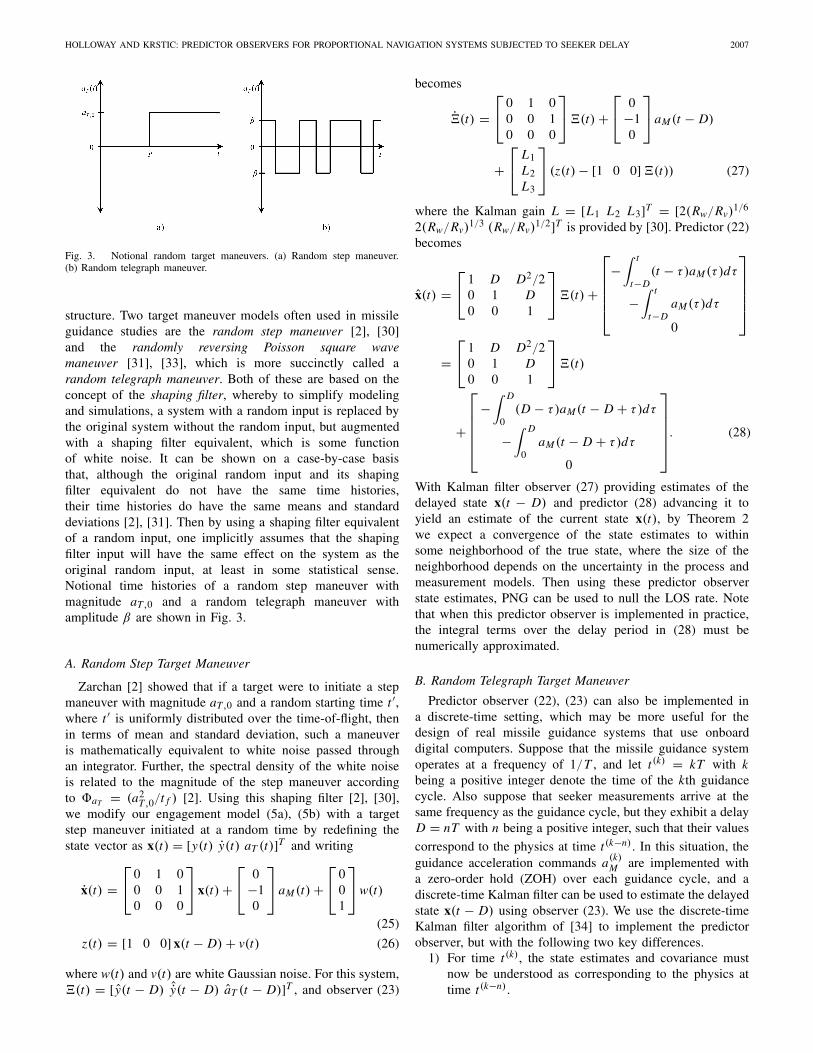
Fig. 3. Notional random target maneuvers. (a) Random step maneuver.(b) Random telegraph maneuver.

structure. Two target maneuver models often used in missileguidance studies are the random step maneuver [2], [30]and the randomly reversing Poisson square wavemaneuver [31], [33], which is more succinctly called arandom telegraph maneuver. Both of these are based on theconcept of the shaping filter, whereby to simplify modelingand simulations, a system with a random input is replaced bythe original system without the random input, but augmentedwith a shaping filter equivalent, which is some functionof white noise. It can be shown on a case-by-case basisthat, although the original random input and its shapingfilter equivalent do not have the same time histories,their time histories do have the same means and standarddeviations [2], [31]. Then by using a shaping filter equivalentof a random input, one implicitly assumes that the shapingfilter input will have the same effect on the system as theoriginal random input, at least in some statistical sense.Notional time histories of a random step maneuver withmagnitude aT ,0 and a random telegraph maneuver withamplitude β are shown in Fig. 3.

A. Random Step Target Maneuver

Zarchan [2] showed that if a target were to initiate a stepmaneuver with magnitude aT ,0 and a random starting time t ′,where t ′ is uniformly distributed over the time-of-flight, thenin terms of mean and standard deviation, such a maneuveris mathematically equivalent to white noise passed throughan integrator. Further, the spectral density of the white noiseis related to the magnitude of the step maneuver accordingto aT = (a2

T ,0/t f ) [2]. Using this shaping filter [2], [30],we modify our engagement model (5a), (5b) with a targetstep maneuver initiated at a random time by redefining thestate vector as x(t) = [y(t) y(t) aT (t)]T and writing

x(t) =⎡⎣ 0 1 0

0 0 10 0 0

⎤⎦ x(t) +

⎡⎣ 0

−10

⎤⎦ aM (t) +

⎡⎣ 0

01

⎤⎦w(t)

(25)

z(t) = [1 0 0] x(t − D) + v(t) (26)

where w(t) and v(t) are white Gaussian noise. For this system,�(t) = [y(t − D) ˆy(t − D) aT (t − D)]T , and observer (23)

becomes

�(t) =⎡⎣ 0 1 0

0 0 10 0 0

⎤⎦�(t) +

⎡⎣ 0

−10

⎤⎦ aM (t − D)

+⎡⎣ L1

L2L3

⎤⎦ (z(t) − [1 0 0] �(t)) (27)

where the Kalman gain L = [L1 L2 L3]T = [2(Rw/Rv)1/6

2(Rw/Rv)1/3 (Rw/Rv)

1/2]T is provided by [30]. Predictor (22)becomes

x(t) =⎡⎣ 1 D D2/2

0 1 D0 0 1

⎤⎦�(t) +

⎡⎢⎢⎢⎢⎣

−∫ t

t−D(t − τ )aM (τ )dτ

−∫ t

t−DaM (τ )dτ

0

⎤⎥⎥⎥⎥⎦

=⎡⎣ 1 D D2/2

0 1 D0 0 1

⎤⎦�(t)

+

⎡⎢⎢⎢⎢⎣

−∫ D

0(D − τ )aM(t − D + τ )dτ

−∫ D

0aM (t − D + τ )dτ

0

⎤⎥⎥⎥⎥⎦. (28)

With Kalman filter observer (27) providing estimates of thedelayed state x(t − D) and predictor (28) advancing it toyield an estimate of the current state x(t), by Theorem 2we expect a convergence of the state estimates to withinsome neighborhood of the true state, where the size of theneighborhood depends on the uncertainty in the process andmeasurement models. Then using these predictor observerstate estimates, PNG can be used to null the LOS rate. Notethat when this predictor observer is implemented in practice,the integral terms over the delay period in (28) must benumerically approximated.

B. Random Telegraph Target Maneuver

Predictor observer (22), (23) can also be implemented ina discrete-time setting, which may be more useful for thedesign of real missile guidance systems that use onboarddigital computers. Suppose that the missile guidance systemoperates at a frequency of 1/T , and let t(k) = kT with kbeing a positive integer denote the time of the kth guidancecycle. Also suppose that seeker measurements arrive at thesame frequency as the guidance cycle, but they exhibit a delayD = nT with n being a positive integer, such that their values

correspond to the physics at time t(k−n) . In this situation, theguidance acceleration commands a(k)

M are implemented witha zero-order hold (ZOH) over each guidance cycle, and adiscrete-time Kalman filter can be used to estimate the delayedstate x(t − D) using observer (23). We use the discrete-timeKalman filter algorithm of [34] to implement the predictorobserver, but with the following two key differences.

1) For time t(k), the state estimates and covariance mustnow be understood as corresponding to the physics attime t(k−n) .


2) In the time updates, the guidance command fromtime t(k−n) must be used rather than from time t(k), sincethe filter equations estimate the delayed state x(t − D)and therefore require the input for that earlier time ratherthan the current one.

Then, since guidance requires estimates of states correspond-ing to the physics at time t(k), the Kalman filter estimatesfor the delayed state must be advanced up to time t(k) usingpredictor formula (22).

Singer [33] also used the shaping filter technique andintroduced an engagement model and discrete-time Kalmanfilter for a target maneuvering in the form of a randomtelegraph signal, which for some applications may be a moreaccurate model of target maneuver than (25). In terms ofmean and standard deviation, the random telegraph signalis mathematically equivalent to an exponential decay excitedby white Gaussian noise [31], [33]. Then defining the statevector as before as x(t) = [y(t) y(t) aT (t)]T , we model anengagement with a random telegraph maneuver as

x(t) =⎡⎣ 0 1 0

0 0 10 0 − α

⎤⎦ x(t)+

⎡⎣ 0

−10

⎤⎦ aM (t)+

⎡⎣ 0

01

⎤⎦w(t) (29)

where α is the inverse of the target maneuver exponentialdecay time constant, w(t) is white Gaussian noise, and weagain use (26) to model the seeker dynamics. The correlationfunction of the process noise satisfies σ 2

w(t) = 2ασ 2mδ(t),

where σ 2m is the variance of the target maneuver acceleration

and δ(t) is the Dirac delta function [33]. Because they arelengthy, we refer the reader to [33] for the discrete-timeKalman filter equations corresponding to (29). Appendix Cshows that for a discrete-time guidance and control systemwith sample period T , state predictor (22) for this engagementmodel is

x(k) =

⎡⎢⎢⎢⎣

1 D1

α2 [−1 + αD + e−αD]0 1

1

α[1 − e−αD]

0 0 e−αD

⎤⎥⎥⎥⎦ x(k−n)

+

⎡⎢⎢⎢⎢⎢⎢⎣

T 2n∑

j=1

(1

2− j

)a(k− j )

M

−Tn∑

j=1

a(k− j )M

0

⎤⎥⎥⎥⎥⎥⎥⎦

. (30)

Now having predictor observer state estimates for time t(k),a pulsed form of PNG is issued through the ZOH to nullthe LOS rate. In this paper, we assumed perfect bang-bangpulses having duration T and magnitude equal to the guidancecommand a(k)

M .It is also interesting to note that after invoking reasonable

assumptions, a discrete-time version of predictor formula (22)reproduces the velocity feed-forward formula introducedin [14] to compensate for sensor processing delays interminal guidance of exoatmospheric interceptors. In [14],delayed seeker measurements and Kalman filter estimateswere propagated forward in time over delay periods using

TABLE I

SCALINGS FOR NONDIMENSIONAL VARIABLES

V measurements from an onboard inertial measurement unitto synchronize state estimates with the guidance cycle. Thevelocity feed-forward formula for the LOS rate took the form

λ(k+1) =(

1 + 2T

t(k)go

)λ(k) − V (k)

Vclt(k)go

. (31)

This formula was to be applied recursively over the delayperiods that were assumed to be equal to integer multiples ofguidance cycles. Although Hablani [14] outlined other meansof deriving (31), it can also be obtained using (22) if the2T/t(k)

go term is ignored, which is often done in practice.We provide a short proof of this in Appendix D. Our workhere corroborates the use of (31) for tactical missiles byshowing that the method is in some sense equivalent to theclassical predictor observer, which we have shown to be ISSwith respect to bounded target maneuvers and measurementdisturbances.

C. Numerical Simulations

We illustrate our examples through numerical simulations.For all simulations, we used nondimensional equations andparameters to display results for a variety of physical situationssimultaneously. We denote all nondimensional variables byan overbar ( ¯ ) using the scalings summarized in Table I.For both examples, PNG denotes an engagement in whichthe baseline undelayed PNG law with Kalman filter is used,PNG/D denotes using the same PNG law and Kalman filtersubjected to a seeker delay, and PNG/DC denotes using thenew predictor observer guidance law to compensate for thesame seeker delay present in the PNG/D simulation. Theconvergence behavior of the observers and guidance lawswill be illustrated in the time histories of state variables,and the overall performance of the guidance laws will bequantified in terms of the miss distance M � y(t0 + t f ) andthe cumulative velocity increment V �

∫ t0+t ft0

|aM (τ )|dτ ,which is a measure of the missile guidance and control effortthat is often used in missile guidance studies. We used aclassical fourth-order Runge–Kutta algorithm with a time stepof t = 10−3 to advance the engagements through time and athird-order trapezoidal quadrature rule to approximate integralsin the predictor formulas. We initialized the state estimatesto zero.

For the random step target maneuver example, Fig. 4illustrates a single simulation with sample pseudorandom noisesequences for the seeker noise (v(t)) in (26) and the inputto the random step target maneuver shaping filter (w(t))in (25). Fig. 4 results from using y(0) = 0.0, ¯y(0) = 0.10,


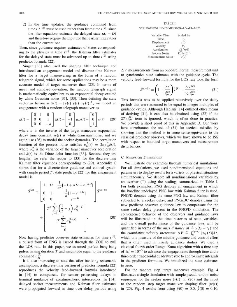
Fig. 4. State and state estimate time histories for random step target maneuverengagement with y(0) = 0.0, ¯y(0) = 0.10, N ′ = 3, and D = 0.25.Est denotes the state estimates of the guidance laws.

and target maneuver shaping filter variance σw = 0.566.The seeker noise has an angular standard deviation ofσλ = 2.0 mrad, which results in a decreasing vertical dis-placement standard deviation of σv = σλr(t). The delayin the seeker measurement is D = 0.25 and N ′ = 3.These parameters represent (among others) an engagementin which r0 = 2000 m, Vcl = 1000 m/s, t f = 2.0 s, andλ(0) = 0.05 mrad/s, and the target initiates a step maneuverof 200 m/s2 at some random time t ′ ∈ [t0, t0 + t f ]. Notethat in practice, a delay of this size would be consideredquite large, since it is one quarter the duration of t f . Forthis sample simulation, the baseline PNG law achieved amiss distance of M = 1.49759 × 10−4 and a cumulativevelocity increment of V = 0.235573, which translates intoM = 0.299518 m and V = 235.573 m/s, respectively.Fig. 4 shows that without compensation, the seeker delaydestabilized the Kalman filter, resulting in a diverging y forPNG/D. However, PNG/DC was able to compensate for thedelay, stabilizing the Kalman filter and thereby driving ytoward zero under the PNG law. PNG/DC resulted in a missdistance of M = −4.28094×10−3 (M = −8.56189 m) versusM = −0.127572 (M = −255.144 m) for PNG/D. FromFig. 5, we see that this reduced miss distance came at thecost of greater V versus the baseline PNG.

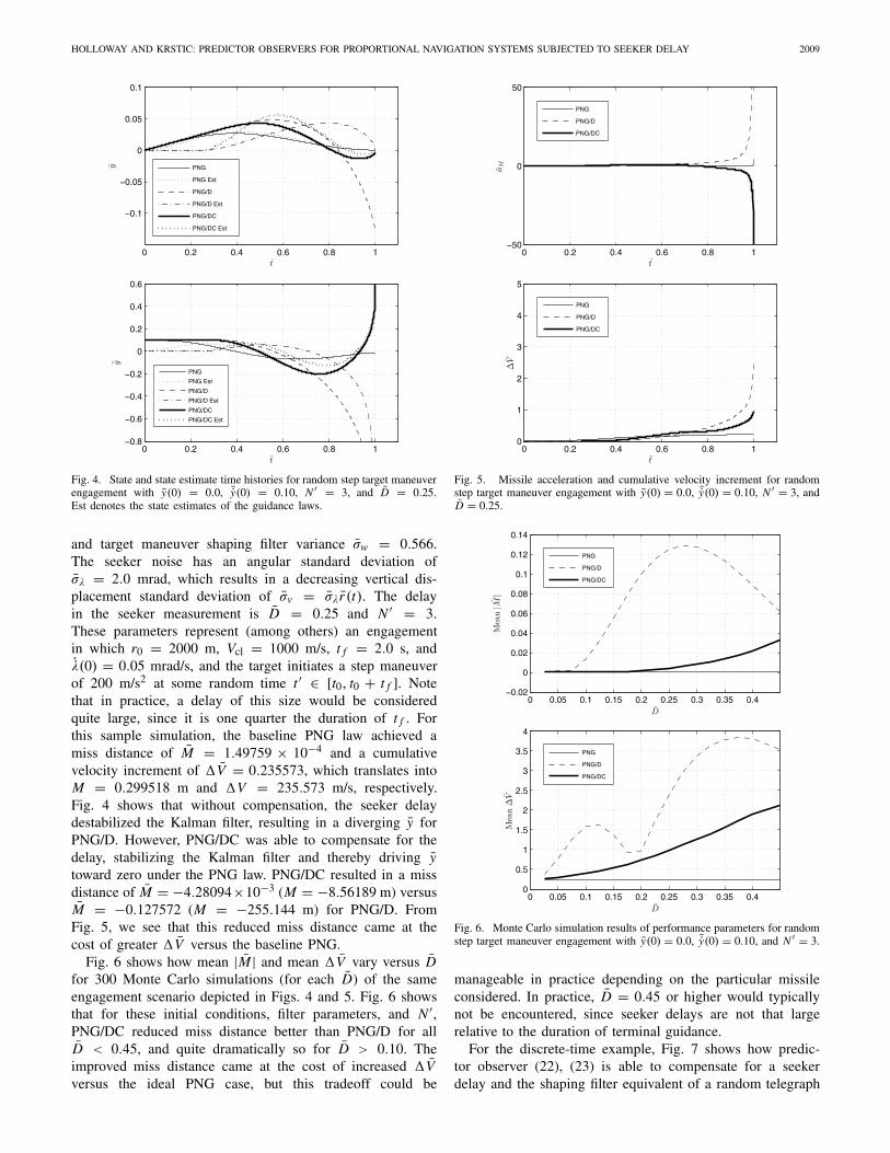
Fig. 6 shows how mean |M| and mean V vary versus Dfor 300 Monte Carlo simulations (for each D) of the sameengagement scenario depicted in Figs. 4 and 5. Fig. 6 showsthat for these initial conditions, filter parameters, and N ′,PNG/DC reduced miss distance better than PNG/D for allD < 0.45, and quite dramatically so for D > 0.10. Theimproved miss distance came at the cost of increased Vversus the ideal PNG case, but this tradeoff could be

Fig. 5. Missile acceleration and cumulative velocity increment for randomstep target maneuver engagement with y(0) = 0.0, ¯y(0) = 0.10, N ′ = 3, andD = 0.25.

Fig. 6. Monte Carlo simulation results of performance parameters for randomstep target maneuver engagement with y(0) = 0.0, ¯y(0) = 0.10, and N ′ = 3.

manageable in practice depending on the particular missileconsidered. In practice, D = 0.45 or higher would typicallynot be encountered, since seeker delays are not that largerelative to the duration of terminal guidance.

For the discrete-time example, Fig. 7 shows how predic-tor observer (22), (23) is able to compensate for a seekerdelay and the shaping filter equivalent of a random telegraph


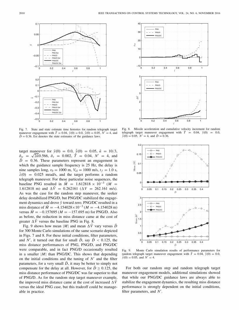
Fig. 7. State and state estimate time histories for random telegraph targetmaneuver engagement with T = 0.04, y(0) = 0.0, ¯y(0) = 0.05, N ′ = 4, andD = 0.36. Est denotes the state estimates of the guidance laws.

target maneuver for y(0) = 0.0, ¯y(0) = 0.05, α = 10/3,σw = √

2α0.566, σv = 0.002, T = 0.04, N ′ = 4, andD = 0.36. These parameters represent an engagement inwhich the guidance sample frequency is 25 Hz, the delay isnine samples long, r0 = 1000 m, Vcl = 1000 m/s, t f = 1.0 s,λ(0) = 0.025 mrad/s, and the target performs a randomtelegraph maneuver. For these particular noise sequences, thebaseline PNG resulted in M = 1.612818 × 10−3 (M =1.612818 m) and V = 0.262161 ( V = 262.161 m/s).As was the case for the random step maneuver, the seekerdelay destabilized PNG/D, but PNG/DC stabilized the engage-ment dynamics and drove y toward zero. PNG/DC resulted in amiss distance of M = −4.154028×10−3 (M = −4.154028 m)versus M = −0.157695 (M = −157.695 m) for PNG/D. Alsoas before, the reduction in miss distance came at the cost ofgreater V versus the baseline PNG in Fig. 8.

Fig. 9 shows how mean |M| and mean V vary versus Dfor 300 Monte Carlo simulations of the same scenario depictedin Figs. 7 and 8. For these initial conditions, filter parameters,and N ′, it turned out that for small D, say D < 0.125, themiss distance performances of PNG, PNG/D, and PNG/DCwere comparable, and in fact PNG/D occasionally resultedin a smaller |M| than PNG/DC. This shows that dependingon the initial conditions and the tuning of N ′ and the filterparameters, for a very small D, it may be better to simply notcompensate for the delay at all. However, for D ≥ 0.125, themiss distance performance of PNG/DC was far superior to thatof PNG/D. As for the random step target maneuver example,the improved miss distance came at the cost of increased Vversus the ideal PNG case, but this tradeoff could be manage-able in practice.

Fig. 8. Missile acceleration and cumulative velocity increment for randomtelegraph target maneuver engagement with T = 0.04, y(0) = 0.0,¯y(0) = 0.05, N ′ = 4, and D = 0.36.

Fig. 9. Monte Carlo simulation results of performance parameters forrandom telegraph target maneuver engagement with T = 0.04, y(0) = 0.0,¯y(0) = 0.05, and N ′ = 4.

For both our random step and random telegraph targetmaneuver engagement models, additional simulations showedthat while our PNG/DC guidance laws are always able tostabilize the engagement dynamics, the resulting miss distanceperformance is strongly dependent on the initial conditions,filter parameters, and N ′.


VI. CONCLUSION

We demonstrated the potential for predictor observers toimprove the stability and performance of PNG systems sub-jected to seeker delay in the near-collision course. We provedthat a classical predictor observer for linear time-delay sys-tems is ISS with respect to bounded target maneuvers andbounded measurement disturbances, and further showed howthe predictor observer can be implemented as a Kalman filterfor the delayed state augmented with a predictor. Using PNGlaws with Kalman filter observers as baselines, numericalsimulations showed that when PNG systems are subjectedto seeker delay, our predictor observer guidance laws areable to stabilize the engagement dynamics and reduce missdistance compared with the baseline guidance laws, whichhave no delay compensation. In practice, the performance ofthe predictor observer Kalman filters will depend on the initialconditions of the engagement and the tuning of N ′ and theKalman filter parameters.

APPENDIX APROOF OF THEOREM 1

Proof: In the near-collision course, PNG can beexpressed as

aM (t) = N ′Vcld

dt

(y(t)

r(t)

). (32)

Assuming a nonmaneuvering target, engagement kinemat-ics (3) reduce to

y(t) = −N ′Vcld

dt

(y(t)

r(t)

). (33)

Integration of (33) gives

y(t) +(

N ′Vcl

r(t)

)y(t) = y0 + N ′Vcl

y0r0

� C (34)

which is a first-order linear ordinary differentialequation (ODE) for y(t). We solve it by multiplyingboth sides by an integrating factor and then integrating. Theintegrating factor is

I (t) = e∫ t

t0

N ′Vclr(τ ) dτ = e

∫ tt0

N ′Vclr0−Vcl(τ−t0) dτ

= eln(

r0r0−Vcl(t−t0)

)N ′

=(

r0

r0 − Vcl(t − t0)

)N ′

. (35)

Multiplying (34) by I (t) gives

d

dt[I (t)y(t)] =

(r0

r0 − Vcl(t − t0)

)N ′

C (36)

and then integration results in

y(t) = y0

(r0 − Vcl(t − t0)

r0

)N ′

+(

r0 − Vcl(t − t0)

r0

)N ′∫ t

t0

(r0

r0 − Vcl(θ − t0)

)N ′

Cdθ.

(37)

For any constant C , integration by substitution shows that

∫ t

t0

(r0

r0−Vcl(θ − t0)

)N ′

Cdθ = − C

Vcl(1 − N ′)

(r0

r(t)

)N ′

r(t)

+ Cr0

Vcl(1 − N ′)(38)

where the integration requires N ′ = 1. Using this fact, aftersubstituting in C = y0 + N ′Vcl(y0/r0) from (34) and reducingthrough algebra, we find that the solution to y(t) is

y(t) = 1

1 − N ′

(r(t)

r0

){[y0 + r0

Vcly0

](r(t)

r0

)N ′−1

−N ′ y0 − r0

Vcly0

}. (39)

The solution is verified by first differentiating to find y(t)

y(t) = 1

1 − N ′

{[− N ′Vcl

r0y0 − N ′ y0

](r(t)

r0

)N ′−1

+ N ′Vcl

r0y0 + y0

}(40)

and then substituting y(t) and y(t) back into (34).It is more convenient to express the solutions to

y(t) and y(t) in matrix form. For a general linear time-varyingsystem with state x(t) and input u(t)

x(t) = A (t)x(t) + B(t)u(t) (41)

the general solution is provided by the variation of parameterformula

x(t) = (t, t0)x(t0) +∫ t

t0(t, θ)B(θ)u(θ)dθ (42)

where x(t0) is the initial condition of the state and (t, t0)is the state transition matrix, defined as the matrix thatsatisfies

d

dt(t, t0) = A (t)(t, t0) (43a)

(t0, t0) = I. (43b)

For the state x(t) = [y(t) y(t)

]T, we have already found

(t, t0) by solving first-order ODE (34). For notational con-venience, we factor out the 1/1 − N ′ and rewrite the statetransition matrix as

(t, t0) = 1

1 − N ′ �(t, t0) (44)

where �(t, t0) is the state transition matrix that satisfies

d

dt�(t, t0) = A (t)�(t, t0) (45a)

�(t0, t0) = (1 − N ′)I. (45b)

Then by inspection of (39) for y(t) and (40) for y(t),the elements of �(t, t0) are obtained, and the theorem isproved. �


APPENDIX BPROOF OF THEOREM 2

Proof: Define the state estimation error as

x(t) � x(t) − x(t)

= x(t) − eF D�(t) −∫ t

t−DeF(t−τ )G1u(τ )dτ. (46)

Rewriting the first term using the variation of parameterformula, this becomes

x(t) = eF D(x(t−D) − �(t))+∫ t

t−DeF(t−τ )G2w(τ )dτ. (47)

Differentiating (47) and reducing then gives

˙x(t) = eF D(F − L H )e−F D[

x(t) −∫ t

t−DeF(t−τ )G2w(τ )dτ

]

− eF D LG3v(t)

+∫ t

t−DFeF(t−τ )G2w(τ )dτ + G2w(t). (48)

Since (F − L H ) is Hurwitz, given some Q = QT > 0, thereexists some P = PT > 0 such that P is the solution to theLyapunov equation

P(F − L H) + (F − L H)T P = −Q. (49)

Using this P , define the Lyapunov function candidate

V [x(t)] = x(t)T e−F T D Pe−F D x(t). (50)

The derivative of V [x(t)] along the trajectory of x(t) is

V [x(t)] = ˙x(t)T e−F T D Pe−F D x(t) + x(t)T e−F T D Pe−F D ˙x(t)

= x(t)T {e−F T D(F − L H )T Pe−F D

+ e−F T D P(F − L H )e−F D}x(t)

− 2x(t)T e−F T D P(F − L H )e−F D�(t)

− 2x(t)T e−F T D P LG3v(t)

+ 2x(t)T e−F T D Pe−F D F�(t)

+ 2x(t)T e−F T D Pe−F DG2w(t) (51)

after substituting in (48) and defining

�(t) �∫ t

t−DeF(t−τ )G2w(τ )dτ (52)

for notational convenience. Then using a similarity transfor-mation of (49), we reduce the term in brackets so that

V [x(t)] = −x(t)T e−F T D Qe−F D x(t)

− 2x(t)T e−F T D P(F − L H )e−F D�(t)

− 2x(t)T e−F T D P LG3v(t)

+ 2x(t)T e−F T D Pe−F D F�(t)

+ 2x(t)T e−F T D Pe−F DG2w(t). (53)

Define

Q1 � e−F T D Qe−F D (54)

P1 � e−F T D Pe−F D. (55)

Then from (50), we have

λ(P1)|x(t)|2 ≤ V [x(t)] ≤ λ(P1)|x(t)|2 (56)

where λ(·) and λ(·) denote the minimum and maximumeigenvalues of a matrix, respectively. Then also

V [x(t)] ≤ λ(P1)|x(t)|2 = 1

λ(P−1

1

) |x(t)|2 (57)

and

−x(t)T Q1x(t) ≤ −λ(Q1)|x(t)|2 (58)

−|x(t)|2 ≤ −λ(P−11 )V [x(t)]. (59)

We now use (58), (59), Young’s inequality in the form 2ab ≤γ a2 + (1/γ )b2, γ > 0 with γ = (1/8)λ(Q1), and completionof squares to reduce (53) to

V [x(t)] ≤ −1

2λ(Q1)λ

(P−1

1

)V [x(t)]

+ 8

λ(Q1)|P1 F�(t)|2 + 8

λ(Q1)|P1G2w(t)|2

+ 8

λ(Q1)|e−F T D P(F − L H )e−F D�(t)|2

+ 8

λ(Q1)|e−F T D P LG3v(t)|2. (60)

The squared absolute value quantities can be reduced asfollows. First observe that

|�(t)| ≤∫ t

t−D|eF(t−τ )G2||w(τ )|dτ

≤(

supτ∈[t−D,t ]

|w(τ )|)∫ t

t−D|eF(t−τ )G2|dτ

≤(

supτ∈[0,t ]

|w(τ )|)

|G2|∫ D

0|eFσ |dσ

≤(

supτ∈[0,t ]

|w(τ )|)

|G2|∫ D

0e|F |σ dσ

= |G2||F |

(e|F |D − 1

)(sup

τ∈[0,t ]|w(τ )|

). (61)

Then further

|P1G2w(t)|2 ≤ |P1G2|2|w(t)|2

≤ |P1G2|2(

supτ∈[0,t ]

|w(τ )|)2

= c1

(sup

τ∈[0,t ]|w(τ )|

)2

(62)

|e−F T D P LG3v(t)|2≤ |e−F T D P LG3|2|v(t)|2

≤ |e−F T D P LG3|2(

supτ∈[0,t ]

|v(τ )|)2

= c2

(sup

τ∈[0,t ]|v(τ )|

)2

(63)


|P1 F�(t)|2 ≤ |P1 F |2|�(t)|2

≤ |P1 F |2 |G2|2|F |2 (e|F |D − 1)2

(sup

τ∈[0,t ]|w(τ )|

)2

≤ |P1|2|G2|2(e|F |D − 1)2

(sup

τ∈[0,t ]|w(τ )|

)2

= c3

(sup

τ∈[0,t ]|w(τ )|

)2

(64)

and

|e−F T D P(F − L H)e−F D�(t)|2≤ |e−F T D P(F − L H )e−F D|2|�(t)|2

≤ |e−F T D P(F − L H )e−F D|2 |G2|2|F |2

× (e|F |D − 1)2

(sup

τ∈[0,t ]|w(τ )|

)2

= c4

(sup

τ∈[0,t ]|w(τ )|

)2

(65)

where we have defined

c1 � λ(GT

2 PT1 P1G2

)c2 � λ

(GT

3 LT Pe−F De−F T D P LG3)

c3 � λ(PT

1 P1)λ(GT

2 G2)(

e√

λ(F T F)D − 1)2

c4 �λ(GT

2 G2)

λ(FT F)

(e√

λ(F T F)D − 1)2

× λ(e−F T D(F −L H)TPe−F De−F T D P(F −L H)e−F D)

.

(66)

Substituting the above expressions into (60) reduces to

V [x(t)] ≤ −1

2λ(Q1)λ

(P−1

1

)V [x(t)]

+ 8

λ(Q1)(c1 + c3 + c4)

(sup

τ∈[0,t ]|w(τ )|

)2

+ 8

λ(Q1)c2

(sup

τ∈[0,t ]|v(τ )|

)2

= − c5V [x(t)] + c6

(sup

τ∈[0,t ]|w(τ )|

)2

+ c7

(sup

τ∈[0,t ]|v(τ )|

)2

(67)

with

c5 � 1

2λ(Q1)λ

(P−1

1

)

c6 � 8

λ(Q1)(c1 + c3 + c4)

c7 � 8

λ(Q1)c2. (68)

By multiplying (67) by ec5t and integrating from 0 to t , it canbe shown that

V [x(t)] ≤ V [x(0)]e−c5t + c6

c5

(sup

τ∈[0,t ]|w(τ )|

)2

+ c7

c5

(sup

τ∈[0,t ]|v(τ )|

)2

. (69)

Then using (56) and (69), it follows that:|x(t)|2 ≤ 1

λ(P1)V [x(t)]

≤ 1

λ(P1)

⎧⎨⎩V [x(0)]e−c5t + c6

c5

(sup

τ∈[0,t ]|w(τ )|

)2

+ c7

c5

(sup

τ∈[0,t ]|v(τ )|

)2⎫⎬⎭

≤ λ(P1)

λ(P1)|x(0)|2e−c5t + c6

c5λ(P1)

(sup

τ∈[0,t ]|w(τ )|

)2

+ c7

c5λ(P1)

(sup

τ∈[0,t ]|v(τ )|

)2

= c8|x(0)|2e−c5t + c9

(sup

τ∈[0,t ]|w(τ )|

)2

+ c10

(sup

τ∈[0,t ]|v(τ )|

)2

(70)

with

c8 � λ(P1)

λ(P1)

c9 � c6

c5λ(P1)

c10 � c7

c5λ(P1)

from which it follows that:|x(t)| ≤ √

c8|x(0)|e− 12 c5t + √

c9 supτ∈[0,t ]

|w(τ )|+√

c10 supτ∈[0,t ]

|v(τ )|. (71)

Then by Definition 1, the observer error dynamics are ISSwith respect to w and v. �

APPENDIX CPREDICTOR OBSERVER FOR RANDOM

TELEGRAPH MANEUVER

With time discretized, predictor (22) for Singer engagementmodel (29) becomes

x(k) =

⎡⎢⎢⎢⎣

1 D1

α2 [−1 + αD + e−αD]0 1

1

α[1 − e−αD]

0 0 e−αD

⎤⎥⎥⎥⎦ x(k−n)

+

⎡⎢⎢⎢⎢⎢⎣

−∫ t (k)

t (k−n)(t(k) − η)u(η)dη

−∫ t (k)

t (k−n)u(η)dη

0

⎤⎥⎥⎥⎥⎥⎦

. (72)


The integral terms are rewritten using only discrete-time quan-tities as follows. The guidance command u(k) is implementedwith a ZOH for all k, so it is constant between guidancecycles. Then consider the integral terms broken up into sumsof integrals over each guidance cycle. Taking from the firstequation of (72), for example, from t(k−n) to t(k−n+1)

−∫ t (k)

t (k−n)(t(k)−η)u(η)dη = −u(k−n)

∫ t (k−n+1)

t (k−n)(t(k) − η)dη

−∫ t (k)

t (k−n+1)(t(k)−η)u(η)dη (73)

where we have factored out the u(k−n) since it is constant fort ∈ [t(k−n), t(k−n+1)]. Continuing on, we have

−∫ t (k)

t (k−n)(t(k)−η)u(η)dη = −u(k−n)

∫ t (k−n+1)

t (k−n)(t(k) − η)dη

−u(k−n+1)

∫ t (k−n+2)

t (k−n+1)(t(k) − η)dη

+ · · · − u(k−1)

∫ t (k)

t (k−1)(t(k) − η)dη

= −u(k−n)

∫ (k−n+1)T

(k−n)T(kT − η)dη

−u(k−n+1)

∫ (k−n+2)T

(k−n+1)T(kT − η)dη

+ · · · − u(k−1)

∫ kT

(k−1)T(kT −η)dη.

(74)

Consider∫ b

a(kT − η)dη =

(kTη − 1

2η2

)∣∣∣∣b

a

= kT (b − a) + a2

2− b2

2

= kT (b − a) + 1

2(a + b)(a − b)

= (a − b)

[1

2(a + b) − kT

]. (75)

Then after rewriting (74) with (75) and reducing the resultalgebraically, we arrive at

−∫ t (k)

t (k−n)(t(k) − η)u(η)dη = u(k−n)T 2

(1

2− n

)

+ u(k−n+1)T 2(

1

2− n + 1

)

+ · · · + u(k−1)T 2(

1

2− 1

)

= T 2n∑

j=1

(1

2− j

)u(k− j ). (76)

Similarly, it can be shown that

−∫ t (k)

t (k−n)u(η)dη = −T

n∑j=1

u(k− j ). (77)

Then state predictor (72) for the discrete-time case reduces to

x(k) =

⎡⎢⎢⎢⎣

1 D1

α2 [−1 + αD + e−αD]0 1

1

α[1 − e−αD]

0 0 e−αD

⎤⎥⎥⎥⎦ x(k−n)

+

⎡⎢⎢⎢⎢⎢⎢⎣

T 2n∑

j=1

(1

2− j

)u(k− j )

−Tn∑

j=1

u(k− j )

0

⎤⎥⎥⎥⎥⎥⎥⎦

. (78)

APPENDIX DPREDICTOR DERIVATION OF (31)

For discrete time, the variation of parameters formula canbe written as

x(k+1) = eAT x(k) +∫ t (k+1)

t (k)eA(t (k+1)−τ ) Bu(τ )dτ. (79)

Using spherical coordinates and defining the state asx = [λ λ]T , where λ is the azimuth LOS angle, the statetransition matrix = eAT used in [14] was

=[

1 T0 1 + (2/tgo)T

](80)

which differs from the state transition matrix for rectangularcoordinates by the existence of the term (2T/tgo). This termis sometimes dropped in practice due to the likely errorin the estimation of tgo [14]. If this is done, substituting

the resulting transition matrix and B = [ 0−(1/Vcltgo)

]for

spherical coordinates into (79) and then looking only at theequation for λ result in

λ(k+1) = λ(k) −∫ t (k+1)

t (k)

1

Vcltgo(τ )u(τ )dτ. (81)

Approximating tgo(t) ≈ t(k)go and u(t) ≈ aM (t) then leads to

λ(k+1) = λ(k) − 1

Vclt(k)go

∫ t (k+1)

t (k)aM(τ )dτ. (82)

But now the integral is equal to the acceleration due toguidance and control sensed over the sample period, denotedby V (k) in [14], and thus

λ(k+1) = λ(k) − V (k)

Vclt(k)go

(83)

which is the same as (31) when the term (2T/tgo) is ignored.

ACKNOWLEDGMENT

The authors would like to thank the reviewers for their feed-back, which increased the scope of this work and improvedits presentation.


REFERENCES

[1] P. Zarchan, “When bad things happen to good missiles,” in Proc.AIAA Guid., Navigat., Control Conf., Washington, DC, USA, 1993,pp. 765–773.

[2] P. Zarchan, Tactical and Strategic Missile Guidance, 5th ed.Washington, DC, USA: AIAA, 2007, pp. 12, 32–34, 66–69, 95–96, and163–165.

[3] N. A. Shneydor, Missile Guidance and Pursuit: Kinematics, Dynamicsand Control. Cambridge, U.K.: Woodhead Publishing Limited, 1998,pp. 129–140, 182–185, and 200–202.

[4] J. Shinar and T. Shima, “A game theoretical interceptor guidance law forballistic missile defence,” in Proc. IEEE CDC, Kobe, Japan, Dec. 1996,pp. 2780–2785.

[5] J. Shinar, T. Shima, and A. Kebke, “On the validity of linearized analysisin the interception of reentry vehicles,” in Proc. AIAA Guid., Navigat.Control Conf., Boston, MA, USA, 1998, pp. 1050–1060.

[6] J. Shinar and T. Shima, “Nonorthodox guidance law developmentapproach for intercepting maneuvering targets,” J. Guid., Control, Dyn.,vol. 25, no. 4, pp. 658–666, 2002.

[7] C. Hecht and A. Troesch, “Predictive guidance for interceptors withtime lag in acceleration,” IEEE Trans. Autom. Control, vol. 25, no. 2,pp. 270–274, Apr. 1980.

[8] N. Léchevin and C. A. Rabbath, “Backstepping guidance for missilesmodeled as uncertain time-varying first-order systems,” in Proc. ACC,Jul. 2007, pp. 4582–4587.

[9] H.-B. Moon, W.-S. Ra, I.-H. Whang, and Y.-J. Kim, “Optimal guidancecut-off strategy based on closed-form PNG solution for single lagsystem,” in Proc. IEEE IECON, Nov. 2011, pp. 652–657.

[10] P. Gurfil, “Robust guidance for electro-optical missiles,” IEEE Trans.Aerosp. Electron. Syst., vol. 39, no. 2, pp. 450–461, Apr. 2003.

[11] P. Gurfil, “Zero-miss-distance guidance law based on line-of-sight ratemeasurement only,” Control Eng. Pract., vol. 11, no. 7, pp. 819–832,2003.

[12] T. Shima, J. Shinar, and H. Weiss, “New interceptor guidance lawintegrating time-varying and estimation-delay models,” J. Guid., Control,Dyn., vol. 26, no. 2, pp. 295–303, 2003.

[13] V. Y. Glizer and J. Shinar, “Optimal evasion from a pursuer with delayedinformation,” J. Optim. Theory Appl., vol. 111, no. 1, pp. 7–38, 2001.

[14] H. B. Hablani, “Endgame guidance and relative navigation of strategicinterceptors with delays,” J. Guid., Control, Dyn., vol. 29, no. 1,pp. 82–94, 2006.

[15] J. Xu, K.-Y. Lum, and J.-X. Xu, “Analysis of PNG laws with LOSangular rate delay,” in Proc. AIAA Guid., Navigat., Control Conf. Exhibit,2007, pp. 1–17.

[16] K.-Y. Lum, J.-X. Xu, K. Abidi, and J. Xu, “Sliding mode guidance lawfor delayed LOS rate measurement,” in Proc. AIAA Guid., Navigat.,Control Conf. Exhibit, 2008, pp. 1–11.

[17] N. Dhananjay, K.-Y. Lu, and J.-X. Xu, “Proportional navigation withdelayed line-of-sight rate,” IEEE Trans. Control Syst. Technol., vol. 21,no. 1, pp. 247–253, Jan. 2013.

[18] M. Krstic, Delay Compensation for Nonlinear, Adaptive, and PDESystems. Cambridge, MA, USA: Birkhäuser, 2009, pp. 41–52.

[19] N. Bekiaris-Liberis and M. Krstic, Nonlinear Control Under Noncon-stant Delays. Philadelphia, PA, USA: SIAM, 2013.

[20] M. Diagne, F. Couenne, and B. Maschke, “Mass transport equation withmoving interface and its control as an input delay system,” in Proc. 11thIFAC Workshop Time-Delay Syst., Grenoble, France, 2013, pp. 331–336.

[21] J. Holloway and M. Krstic, “A predictor observer for seeker delay in themissile homing loop,” in Proc. 12th IFAC Workshop Time Delay Syst.,Ann Arbor, MI, USA, 2015, pp. 416–421.

[22] K. Watanabe and M. Ito, “An observer for linear feedback control lawsof multivariable systems with multiple delays in controls and outputs,”Syst. Control Lett., vol. 1, no. 1, pp. 54–59, 1981.

[23] J. Klamka, “Observer for linear feedback control of systems withdistributed delays in controls and outputs,” Syst. Control Lett., vol. 1,no. 5, pp. 326–331, 1982.

[24] D.-Y. Rew, M.-J. Tahk, and H. Cho, “Short-time stability of proportionalnavigation guidance loop,” IEEE Trans. Aerosp. Electron. Syst., vol. 32,no. 3, pp. 1107–1115, Jul. 1996.

[25] P. Gurfil, M. Jodorkovsky, and M. Guelman, “Finite time stabilityapproach to proportional navigation systems analysis,” J. Guid., Control,Dyn., vol. 21, no. 6, pp. 853–861, 1998.

[26] H. Khalil, Nonlinear Systems. Englewood Cliffs, NJ, USA:Prentice-Hall, 2002, pp. 144 and 174–180.

[27] M. Krstic, I. Kanellakopoulos, and P. V. Kokotovic, Nonlinear and Adap-tive Control Design. New York, NY, USA: Wiley, 1995, pp. 501–506.

[28] T. Ahmed-Ali, E. Cherrier, and F. Lamnabhi-Lagarrigue, “Cascade highgain predictors for a class of nonlinear systems,” IEEE Trans. Autom.Control, vol. 57, no. 1, pp. 221–226, Jan. 2012.

[29] C. L. Coutinho, T. R. Oliveira, and J. P. V. S. Cunha, “Output-feedbacksliding-mode control via cascade observers for global stabilisation ofa class of nonlinear systems with output time delay,” Int. J. Control,vol. 87, no. 11, pp. 2327–2337, 2014.

[30] F. Nesline and P. Zarchan, “A new look at classical versus mod-ern homing missile guidance,” in Proc. AIAA Guid. Control Conf.,1979, pp. 230–242.

[31] G. M. Siouris, Missile Guidance and Control Systems. New York, NY,USA: Springer-Verlag, 2004, pp. 251–252.

[32] B. D. O. Anderson and J. B. Moore, “Kalman filtering: Whence,what and whither?” in Mathematical System Theory. Berlin, Germany:Springer-Verlag, 1991, pp. 41–54.

[33] R. A. Singer, “Estimating optimal tracking filter performance for mannedmaneuvering targets,” IEEE Trans. Aerosp. Electron. Syst., vol. AES-6,no. 4, pp. 473–483, Jul. 1970.

[34] G. F. Franklin, J. D. Powell, and M. Workman, Digital Control ofDynamic Systems, 3rd ed. Reading, MA, USA: Addison-Wesley, 1998,pp. 389–391.

John Holloway received the B.Sc. degree in physicsand mathematics from Morehead State University,Morehead, KY, USA, in 2004, the B.Sc. degreein mechanical engineering from the University ofKentucky, Lexington, KY, USA, in 2004, undera joint-university, dual-degree program, theM.Sc. degree in mechanical engineering from theUniversity of California at San Diego, La Jolla,CA, USA, in 2006, and the Graduate Certificatein Guidance and Control from Stanford University,Stanford, CA, USA, in 2010. He is currently

pursuing the Ph.D. degree with the University of California at San Diego.He has been a Guidance, Navigation, and Controls Engineer with Engility,

Chantilly, VA, USA, since 2006, where he is involved in performingmodeling and simulation analyses for design validation and verificationof aerospace systems. He was named an Associate Technical Fellow withEngility in 2012.

Miroslav Krstic (F’01) holds the Alspach EndowedChair and is the Founding Director of the CymerCenter for Control Systems and Dynamics withthe University of California at San Diego (UCSD),La Jolla, CA, USA. He serves as an AssociateVice Chancellor for Research with UCSD. He servesas an Editor of two Springer book series. He hasco-authored 11 books on adaptive, nonlinear, andstochastic control, extremum seeking, control of par-tial differential equation systems, including turbulentflows, and control of delay systems.

Prof. Krstic is a fellow of the International Federation of AutomaticControl (IFAC), the American Society of Mechanical Engineers (ASME), theSociety of Industrial and Applied Mathematics (SIAM), and the Institutionof Engineering and Technology (IET), U.K., an Associate Fellow of theAmerican Institute of Aeronautics and Astronautics (AIAA), and a ForeignMember of the Academy of Engineering of Serbia. As a Graduate Student,he won the University of California at Santa Barbara Best Dissertation Awardand Student Best Paper Awards at the IEEE Conference on Decision andControl (CDC) and the American Control Conference (ACC). He has receivedthe Presidential Early Career Award for Scientists and Engineers, the NSFCareer Award, and the ONR Young Investigator Award, the Axelby andSchuck Paper Prizes, the Chestnut Textbook Prize, the ASME Nyquist LecturePrize, and the first UCSD Research Award given to an Engineer. He has alsoreceived the Springer Visiting Professorship at the University of Californiaat Berkeley, Berkeley, CA, USA, the Distinguished Visiting Fellowship ofthe Royal Academy of Engineering, the Invitation Fellowship of the JapanSociety for the Promotion of Science, and the Honorary Professorshipsfrom Northeastern University, Shenyang, China, and Chongqing University,Chongqing, China. He serves as a Senior Editor of the IEEE TRANSACTIONS

ON AUTOMATIC CONTROL and Automatica. He has served as the VicePresident for Technical Activities of the IEEE Control Systems Society andthe Chair of the IEEE Control Systems Society Fellow Committee.

Documents

2002 IEEE TRANSACTIONS ON CONTROL SYSTEMS …