Brownbag Seminar

Monday, January 22, 200112.00-1.00 p.m.

Department of Agricultural and Resource Economics UC Davis

Valuing Benefits of Finnish Forest Biodiversity Conservation –

Logit Models for Pooled Contingent Valuation and

Contingent Rating/Ranking Survey Data*

Juha Siikamäki**

Abstract This paper examines contingent valuation and contingent rating/ranking valuation methods (CV and CR methods) for measuring willingness-to-pay (WTP) for nonmarket goods. Recent developments in discrete choice econometrics using random parameter models are applied to CV and CR data and their performance evaluated in comparison to conventionally used fixed parameter models. A framework for using data pooling techniques to test for invariance between separate sources of data is presented and applied to combined CV and CR data. The empirical application deals with measuring the WTP for conserving biodiversity hotspots in Finnish non-industrial private forests. Results suggest that random coefficient models perform statistically well in comparison to fixed parameter models that sometimes violate the assumptions of conditional logit model. Random parameter models also result in considerably lower WTP estimates than fixed paramater models. Based on the pooled models on combined data, parameter invariance between CV and CR data cannot be uniformly accepted or rejected. Rejecting pooling of the data becomes more likely as more detailed response models are applied.

* Work-in-progress, please do not cite, comments and suggestions welcome.** Ph.D. Candidate, Department of Environmental Science and Policy, University of California, Davis. Email: juha@primal.ucdavis.edu

2.1 Introduction

This paper examines contingent valuation and contingent rating/ranking (CV and CR) methods in

measuring willingness-to-pay (WTP) for nonmarket goods. Recent developments in discrete choice

econometrics using random parameter models are applied to CV and CR data, and their

performance is evaluated in comparison to conventionally used fixed parameter econometric

models. Second, invariance between CV and CR data is examined by data pooling techniques, also

an actively developing research area that has not been previously employed in this context.

Stated preference methods (SP methods) are widely used in measuring economic values related to

the environment. A standard SP application includes conducting surveys, in which respondents are

described hypothetical alternatives, usually policy options, that each result in a certain supply of

nonmarket good, such as environmental quality, for certain costs to respondents. They are asked to

evaluate the alternatives and state their preferences regarding them. The CV is based on asking for

acceptance/refusal of hypothetical payment for implementing a policy alternative; the CR relies on

asking respondents to rate or rank the available alternatives, at the simplest by choosing a preferred

alternative. Obtaining responses for a variety of cost-environmental quality combinations, data with

implicit information on individual tradeoffs between money and environmental quality are

collected. The tradeoffs can be quantified by using discrete choice econometric models, that explain

the observed choices by attributes of policy alternatives and respondents. In essence, they can be

used to measure an individual level exchange rate between a nonmarket good and money.

Willingness to pay (WTP) for changes in the environmental quality can then be calculated using the

estimation results.

Although several stated preference methods are currently in use, their performance and consistency

has not been exhaustively studied. Examples of studies on differences between SP methods include

Desvouges and Smith 1983, Magat et al. 1988, Boxall et al. 1996, Stevens et al. 2000. They all

suggest substantial differences between different SP methods. This is discomforting for SP-

practioners, since all the methods attempt to measure essentially the same tradeoffs between money

and changes in environmental quality and their results should be very similar.

2

Previous studies on differences across SP methods are typically based on fixed parameter discrete

choice models, usually logit models. The assumptions and properties of fixed logit models are

restrictive, but more flexible models with random parameters have been practically unavailable due

to limitations in computing power and simulation based econometric techniques. Both constraints

have recently been greatly relaxed and random parameter models are now possible to be employed

in modeling the discrete choice SP data, as conceptualized and demonstrated for instance by Train’s

(1998) study on recreational fishing site choice and by Layton’s (2000a) work on rankings data.

They conclude that random parameter formulation can significantly improve both the explanatory

power of models and the precision of estimates they result.

The results of random parameter applications suggest that differences between SP should be re-

examined using less restrictive econometric models. More flexible models let us to evaluate if

previous conclusions have resulted from inequalities between different SP data sources, or perhaps

from using overly restrictive econometric models.

Hensher et al. (1999) provide a framework for applying data pooling techniques to test for data

invariance between separate sources of data. Their approach is adopted here and used to test for

equality of CV and CR data. The study demonstrates how data pooling approach can be used in

examining the differences between the SP methods. It enables comparison of separate data sources

already at the estimation stage and provides a useful framework for tests of the differences between

different data sources.

The empirical application deals with measuring WTP for conserving especially valuable habitats

(biodiversity hotspots) in Finnish non-industrial private forests. According to ecologists, protection

of the biodiversity hotspots is particularly important for biodiversity conservation in Finland. The

hotspots cover a total of 1.1 million hectares, that is some 6 % of the Finnish forests. Current

regulations protect some 110.000 hotspot hectares and extending their protection is currently

debated. The relevant policy question is how big portion of the currently unprotected biodiversity

hotspots should be conserved in the future. This study evaluates different conservation policy

alternatives and public’s preferences for them.

3

Forest conservation in Finland is an inexhaustible source of public debates and policy conflicts.

Clearly, management and harvesting of forests are primary reasons for species extinction. Rather

intensive forest management practices over a long period of time have provided country with more

timber resources than ever in the known past. At the same time, substantial losses of old forests and

other important habitats for many currently threatened species have resulted. On the other hand, a

big share of country’s exports still consist of forest products such as paper- and sawmill products.

Economic interests related to forests are therefore evident. Noting further that forests consist mostly

(65-75 %) of small holdings (avg. size 100 acres), owned by private households, and that almost

every 10th Finn owns some areas forests, it is clear that forest conservation policies are of

considerable public interest.

The specific objectives of this paper are to

1) Review and discuss current logit models for the CV and CR data

2) Examine random parameter modeling approach empirically in comparison to fixed parameter

models

3) Test for differences between SP methods by using data pooling methods

4) Analyze WTP estimates for both fixed and random parameter and unpooled and pooled models

for CV and CR data

The rest of the paper is organized as follows: The first section represents the econometric models

for CV and CR data, including fixed and random coefficient models. Next section describes how

data pooling techiques can be used in tests for data invariance across between different stated

preference data sources. The empirical section starts with description of the public survey for

preferences for biodiversity conservation in Finland. Results start with fixed logit models and

continue with the results for random parameter models. After separate estimation of CV and CR

data, the data are pooled and invariance between the CV and CR data tested. The results section is

concluded with presenting the calculated WTP estimates for different models. Last, the results of

study are briefly discussed and concluded. Discussion and conclusion parts are not yet fully

completed.

4

2.2. Econometric Models for Contingent Valuation and Contingent Rating/Ranking Survey

Responses

Econometric models for stated preference surveys are typically based on McFadden’s (1974)

random utility model (RUM). The following section uses RUM as a point of departure for

explaining various econometric models for CV and CR survey responses. The CV section draws

from works by Hanemann (1984), Hanemann et al. (1991), and Hanemann and Kanninen (1996);

the CR section relies on McFadden (1974), Beggs et al. (1981), Chapman and Staelin (1982),

Hausman and Ruud (1987) and on recent works by Train (e.g. 1998), Train and McFadden (2000)

and Layton (2000a).

2.2.1. Random Utility Theoretic Framework for Modeling Individual Choices

Typical stated preference surveys try to measure individual tradeoffs between changes in

environmental quality q and costs A of implementing them. That is accomplished by asking

respondents to state their choices between status quo with zero cost and one or more hypothetical

policy alternatives with altered environmental quality and its costs. Consider an individual i

choosing a preferred alternative from a set of m alternatives, each alternative j providing utility Uij,

that can be additively separated into an unobserved stochastic component ij and a deterministic

component Vij(qj,y-Aj) i.e the restricted indirect utility function that depends only on individual’s

income, y, and environmental quality, q. The utility of alternative j can then be represented as

Uij=Vij(qj,y-Aj)+ij (2.1)

The stochastic ij represents the unobserved factors that affect the observed choices. They can be

related to individual tastes, choice task complicity, or any other factors with significant influence on

choices. They are taken into consideration by individual j choosing between the alternatives, but to

an outside observer, ij remains unobserved and stochastic in the econometric modelling.

Importantly, from the viewpoint of individual making a choice, utility has no stochastic nature.

Choices are based on utility comparisons between the available alternatives and the alternative

providing the highest utility becomes the preferred choice. The probability of person i choosing

alternative j among all the m the alternatives therefore equals the probability that the alternative j

5

provides person i with greater utility Uij than any other available alternative with Uik. It is

determined as

Pij = P (Uij > Uik, k = 1, ..., m, k j), (2.2)

which can be represented as

Pij = P (Vij(q,y-Aj) + ij > Vik (q,y-Ak)+ ik, k = 1, .., m, k j), (2.3)

and rearranged

Pij = P ( ij – ik > Vik(q,y-Ak) – Vij(q,y-Aj), k = 1, .., m, k j) (2.4)

Denoting the difference of random components between alternatives j and k as i = ij –ik, and the

difference between the deterministic components as Vi (.)= Vik (q,y-Ak)– Vij(q,y-Aj), the probability

Pij can be presented as probability

Pij = P (i > Vi(.), k = 1, .., m, k j) (2.5)

Estimating parametric choice models then requires specification of both the distribution of i and the

functional form of Vij. Specification of i determines the probability formulas for the observed

responses; functional form of Vij is employed in estimating the unknown parameters of interest.

Denoting all the exogenous variable of alternative j to ith person as a vector X ij, and the unknown

parameters as a vector , Vij is typically specified as linear in parameters Vij=Xij. The linear

formulation is used in the rest of this study, including the estimated results.

Maximum likelihood methods are typically used in estimating Vij. The maximum likelihood

estimation (MLE) seeks the parameter estimates that have most likely generated the observed data

on choices. The following sections describe response probability formulas for different contingent

valuation (CV) and contingent ranking (CR) models. Response probability formulas can be thought

of as a likelihood function for ith person. Since observations are independent, the likelihood

function for the total sample is simply a sum of individual likelihood functions. The MLE is

typically employed by maximizing a logarithmic transformation of the likelihood function.

6

2.2.2. Logit models for CR data

Assume in the following that random terms i and j are independently and identically distributed,

type I generalized extreme value random variables. It follows in turn that their difference ij is

logistically distributed. Under these assumptions, McFadden (1974) showed that choice probability

Pij in (2.5) is determined as conditional logit model

(2.6)

The log-likelihood function for conditional logit model is

(2.7)

Important features are related to parameter , a scale factor that appears in all the choice models

based on RUM. It links the structure of random terms and the parameter estimates of Vij=Xij. With

data from a single source, the scale factor is typically set equal to one, left out, and parameter vector

estimated given the restricted scale factor. This is necessary for identification; without the

imposed restriction on , neither nor could be identified. However, in combining data from

different sources, the scale factor plays an essential role. Since pooling of CV and CR data plays a

primary role in this analysis, scale paramaters are included in all the described models. The role

scale of factor in pooling different sources of data will be discussed in more detail in section 2.2.5.

Beggs et al (1981) and Chapman and Staelin (1982) extended the conditional logit model to

modeling ranking of alternatives. A rank-ordered logit model treats ranking as m-1 consecutive

conditional choice problems. In other words, it assumes that ranking results from m-1 utility

comparisons, where the highest ranking is given to best alternative (the preferred choice from the

available alternatives), the second highest ranking to best alternative from the remaining m-1

alternatives, third from remaining m-2 alternatives, and so on. The probability of observed ranking

is given by

(2.8)

7

Hausman and Ruud (1987) developed a rank-ordered heteroscedastic logit model that is flexible

enough to take into account possible increases (or decreases) in variance of the random term in the

RUM as the ranking task continues. It is based on formulation with rank-specific scale parameter

that accounts for possible identifies p-1 scale parameters.

(2.9)

The log-likelihood function for rank-ordered logit models (2.8) and (2.9) is

(2.10)

2.2.3. Logit models for CV data

Typical dichotomous choice CV uses a single bounded (SB) discrete choice format. It is based on

asking respondents if they would or would not be willing to pay certain reference amount Bid of

money of their income y for altering environmental quality q. Data consist of binary responses that

result from yes/no answers to CV questions, asking for refusal/acceptance of paying an amount Bid

for some policy alternative. In essence, the CV-method asks respondents to choose between status

quo with utility Ui0(q0) = Vi0(q0) + ei0 and an alternative providing utility Ui1(q1) = Vi1(q1, y-Bid ) +

ei1. Given logistically distributed stochastic term in the RUM, probability of individual i choosing

the alternative with costs Bid and environmental quality q1 is the probability of obtaining a Yes-

answer from person i. Expressing the observed parts of utilities as Vi0 = Xi0 and Vi1 = Xi1, the

probability of Yes-answer is given by conditional logit model with two alternatives (binary choice):

(2.11)

The log likelihood function for the single bounded CV is

(2.12)

In double bounded CV, respondents are asked a follow-up question based on the first response. The

idea is to gather more information on WTP than is possible by asking a single question.

8

Respondents with Yes-answer to the first question (FirstBid) are asked a similar second question,

this time with HighBid > FirstBid. Respondents with No-answer get a second question with

LowBid < FirstBid. Second responses provide more detailed data on individual preferences

between the two alternatives and the choice probabilities can now be determined based on responses

to two separate questions. Four possible response sequences can be observed: Yes-Yes, Yes-No,

No-Yes and No-No. Using the conditional logit model, and denoting the exogenous variables for

FirstBid, HighBid and LowBid by XiFB, XiHB and XiLB, probabilities of different responses are given

by:

P(Yes-Yes) =

P(Yes-No) = (2.13)

P(No-Yes) =

P(No-No) =

Using dummy variables, Iyy, Iyn, Iny, Inn, to indicate Yes-Yes, Yes-No, No-Yes and No-No responses,

the log-likelihood function for double-bounded CV is

(2.14)

2.2.4. Random parameter logit models

Although typically applied to SP data, some undesirable properties and assumptions are embodied

in fixed parameter logit models. First, they are known to overestimate the joint probability of

choosing close substitutes. This is known as the Independence of Irrelevant Alternatives (IIA)

property (McFadden 1974). Second, they are based on the assumption that the random terms ij are

independently and identically distributed, in practice it is more likely that the individual specific

factors influence evaluation of all the available alternatives and make random terms correlated

instead of independent. Third, assuming homogeneous preferences alone is restrictive. Any

9

substantial variation in individual tastes conflicts with this assumption, possibly resulting in

violations in many applications.

Random parameter logit (RPL) models have been proposed to overcome possible problems of the

fixed parameter choice models (e.g. Revelt and Train 1998, Train 1998, Layton 2000). The RPL is

specified similarly as the fixed parameter models, except that the parameters now vary in

population rather than are the same for each person. Utility is expressed as a sum of population

mean b, individual deviation , which accounts for differences in individual taste from the

population mean, and an unobserved i.i.d. random term . Total utility for person i from choosing

the alternative j is determined as

Uij = Xijb+Xiji+ij (2.15)

where Xijb and Xiji+ij are the observed and unobserved parts of utility. Utility can also be

expressed in form Xij(b+i)+ij, which is easily comparable to fixed parameter models. The only

difference is that previously fixed now varies across people as i=b+ i.

Although RPL models account for heterogeneous preferences via parameter i, individual tastes

deviations are neither observed nor estimated. RPL models aim at finding the different moments,

for instance the mean and the deviation, of the distribution of , from which each i is drawn.

Parameters vary in population with density f(|), with denoting the parameters of density. Since

actual tastes are not observed, the probability of observing a certain choice is determined as an

integral of the appropriate probability formula over all the possible values of weighted by its

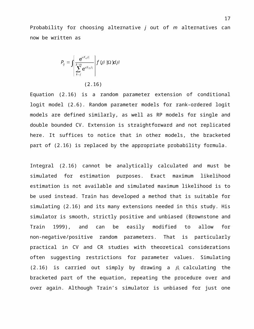
density. Probability for choosing alternative j out of m alternatives can now be written as

(2.16)

Equation (2.16) is a random parameter extension of conditional logit model (2.6). Random

parameter models for rank-ordered logit models are defined similarly, as well as RP models for

single and double bounded CV. Extension is straightforward and not replicated here. It suffices to

notice that in other models, the bracketed part of (2.16) is replaced by the appropriate probability

formula.

10

Integral (2.16) cannot be analytically calculated and must be simulated for estimation purposes.

Exact maximum likelihood estimation is not available and simulated maximum likelihood is to be

used instead. Train has developed a method that is suitable for simulating (2.16) and its many

extensions needed in this study. His simulator is smooth, strictly positive and unbiased (Brownstone

and Train 1999), and can be easily modified to allow for non-negative/positive random parameters.

That is particularly practical in CV and CR studies with theoretical considerations often suggesting

restrictions for parameter values. Simulating (2.16) is carried out simply by drawing a i, calculating

the bracketed part of the equation, repeating the procedure over and over again. Although Train’s

simulator is unbiased for just one draw of i, it’s accuracy is increased with the number of draws.

Using R draws of i from f(|), the simulated probability of (2.16) is

(2.17)

Simulator (2.17) can be extended to rank-ordered logit model (see Layton 2000a) and to logit

models for single and double bounded CV. The only change required is replacing the R times

summed portion of (2.17) with the rank-ordered, single bounded CV or double bounded CV

probability formulas, as expressed by (2.8), (2.11), and (2.14). In estimating mean and variance for

distribution of , (2.17) can be employed by defining Xij ir=Xij(b+eir), where b and are estimated

mean and deviation parameters and eir a standard normal deviate for rth replication for individual i.

Estimation of parameters is carried out by maximizing simulated likelihood function, determined by

the appropriate simulated response probability formula, in a much similar way as for fixed logit

models. The simulated log-likelihood function for random parameter conditional logit model (2.17)

is

(2.18)

Formulas for other simulated response probabilities and their log-likelihood formulas are

summarized in Appendix.

It is worth noting that RPL models are also flexible in approximating the response models resulting

from other distributional assumptions, such as probit models with normality of random term in RU

model assumed. In fact, McFadden and Train (2000) show that any discrete choice model derived

11

from random utility maximization can be approximated arbitrarily close by random parameter

multinomial logit model.

2.2.5. Pooling Data

The scale of estimated parameters in all the choice models based on RUM is related to the

magnitude of the random component in the RU model. The scale factor relates the estimates with

the random component and is inversely related to the variance of random component in the RUM.

Using a single source of data, is typically set equal to one since it cannot be identified. The

estimated vector of coefficients gets therefore confounded with constant . This in turn makes

absolute values of parameter estimates incomparable between different data sets, only the ratios of

coefficients are comparable across different sources of data (Swait and Louviere 1993).

Consider n separate sources of stated preference data, such as survey data using CV and CR.

Normalizing scale factors equal to one in estimation of separate data sources, each data q=1,...,n

provides us with parameter estimates q. Denoting the scale parameters of different data sources

with q, n vectors qq of parameter estimates results. Pooling n sources of data, it is possible to

identify n-1 scale parameters for different data sources. Fixing one scale factor, say 1=1, the rest n-

1 estimated scale parameters are inverse variance ratios relative to reference data source (Hensher et

al. 1999).

Studying parameter invariance across CV and CR data is in the focus of this paper. Denote vector of

CV and CR estimates by CVCV and CRCR. When pooling CV and CR, fixing CV =1 and

estimating CR accounts for possible differences in the variance of random terms between the CV

and CR data. To test parameter invariance between the CV and CR data, models with and without

restriction CV =CR are estimated on pooled data. Likelihood ratio tests can then be applied to

accept/reject the imposed parameter restriction. If the null hypothesis cannot be rejected, data

generation processes can be considered generated by the same taste parameters but still have

variance differences. Restricting also CR=1, provides an even more strict test of data invariance,

since it tests for both parameter and random component invariance. If not rejected, the two data sets

could be considered similar and absolute parameter estimates comparable across data sources.

12

2.3. The Data

Data were collected using a mail survey, sent out in spring 1999 to a random sample of 1740 Finns

between 18-75 years of age. The sample was randomly divided into two subsamples of 840 and 900

respondents. The first subsample received a double bounded CV questionnaire and the second

subsample a CR questionnaire.

Questionnaire started with questions about respondents attitudes on how important different aspects

of forests, such as their economic importance and different uses (timber production, recreation,

nature conservation etc) should be in formulating forest policy. Next, respondents were asked to

state how important issues such as public healthcare, education, employment, economic growth,

nature conservation and equal income distribution should be in formulating public policies in

general. Thereafter, respondents were asked still a number of attitude questions about forest

conservation, landowners’ and public’s responsibilities in conservation and acceptability of forcing

landowners to protect forests by regulatory approaches. Next section of the questionnaire included

the valuation questions, described in more detail later on. The questionnaire was concluded with

questions on respondent’s socioeconomic background.

While designing the survey, questionnaire versions went through several rounds of modifications

and reviews by accustomed SP-practioners, as well as economists, forresters and ecologists with

expertise in survey methods and/or biodiversity conservation. After hearing their comments,

questionnaires were tested by personal interviews and a pilot survey (n=100) and modified based on

their results. Survey was mailed out in May 1999. A week after the first mailing, everybody in the

sample was sent a reminder card. Two more rounds of reminders with a complete questionnaire

were sent to non-respondents in June-July. The CV and CR surveys resulted in 48,9 % and 50 %

response rates, respectively. After censoring for all the missing answers to valuation questions, 376

CV and 391 CR responses were available for further examination.

The WTP is measured for three hypothetical conservation programs: Increasing conservation from

current 110.000 hectares to (1) 275.000 hectares, (2) 550.000 hectares and (3) 825.000 hectares.

13

The new alternatives correspond to protection of 25 %, 50 % and 75 % of all the available

biodiversity hotspots. In designing the survey, special attention was paid to formulating

conservation policy scenarios so that they were policy relevant, credible and intuitive to understand.

A page long, easy to read section in the questionnaire explained different conservation programs

and their details.

Table 2.3.1. Four possible conservation projects presented for the CR respondents.

Conservation Project Total area under conservation

Proportion of conserved of all the Finnish forests

1. Current regulation, no new conservation 120.000 hectares 0.6 percent

2. Increasing conservation to cover one fourth (25%) of the biodiversity hotspots

275.000 hectares 1.5 percent

3. Increasing conservation to cover half (50%) of the biodiversity hotspots

550.000 hectares 3 percent

4. Increasing conservation to cover three fourths (75%) of the biodiversity hotspots

705.000 hectares 4.5 percent

The CR survey described to respondents the status quo and all three hypothetical programs of

setting aside additional 155.000, 430.000 and 705.000 hectares of hotspots for a 30-year1 long

conservation. Table 2.3.1 describes how the conservation programs were summarized in the CR

questionnaire. Using scale from 0 to 10, each respondent was asked to rate all the four programs.

Note here that the respondents are not asked to hypothetically buy any forest areas; they are simply

asked to express their preferences regarding different conservation programs that would each result

in different conservation levels and costs to their households. The three hypothetical programs were

assigned costs using the same variation across the respondents and the conservation programs as in

the CV survey, described in more detail later on.

The respondents of CV questionnaires were divided into two groups. First group was asked to state

their WTP for the first two policy alternatives, i.e. 155.000 and 430.000 hectares as described in

Table 1, and the second group for 430.000 and 705.000 hectare alternatives. Each respondent was

asked two separate CV questions, and responses for 50 % conservation were therefore collected by

1 The length of protection is determined as 30 years simply because the current conservation policy programs and initiatives are based on 30 year protection.

14

both first and second WTP questions, depending on respondent’s subsample. A double bounded

format of the CV was applied in all CV questionnaires. The bid vector in CV survey consisted of

first bids between USD 4-500 (FIM 25-3000) and the follow-up bids between USD 2-800, with

seven different starting bids. Same bid amounts appeared for some respondents as first bids and for

some as second bids, and bids for different levels of conservation were chosen from across the full

vector of bids.

The final survey consisted of 29 different questionnaire versions, of which 14 were using the CV

and 15 the CR. In both types of surveys, the WTP was measured as an increase in the annual tax

burden of the household. Except for the valuation question, the CV and CR questionnaires were

similar.

2.4. Results

The next sections first report and discuss the results of fixed and random parameter logit models

separately for CV and CR data. After separate estimation of the CV and CR data, the data are

combined and invariance between CV and CR data is tested. All the results are based on maximum

likelihood estimation of the models, that were described in earlier sections of this paper and

programmed and estimated in GAUSS.

Estimation uses a dummy specification for conservation programs. In other words, conservation is

modeled as three different conservation programs, not as a continuous variable of conserved

hectares under each policy alternative. This results in several benefits: First, the specification is very

flexible and does not restrict the value function for conservation to follow any certain functional

form, letting it take practically any form instead. Second, the WTP for different conservation

programs can now be calculated simply as ratios of the estimated parameters. Third, separate

dummies can be used in measuring variances of taste parameters for different extents of

conservation, which is not the case when specifying conservation level as a continuous variable.

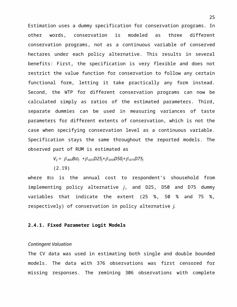
Specification stays the same throughout the reported models. The observed part of RUM is

estimated as

Vij = iBIDBIDj + iD25D25j+ iD50D50j+ iD75D75j (2.19)

15

where BID is the annual cost to respondent’s shousehold from implementing policy alternative j, and

D25, D50 and D75 dummy variables that indicate the extent (25 %, 50 % and 75 %, respectively) of

conservation in policy alternative j.

2.4.1. Fixed Parameter Logit Models

Contingent Valuation

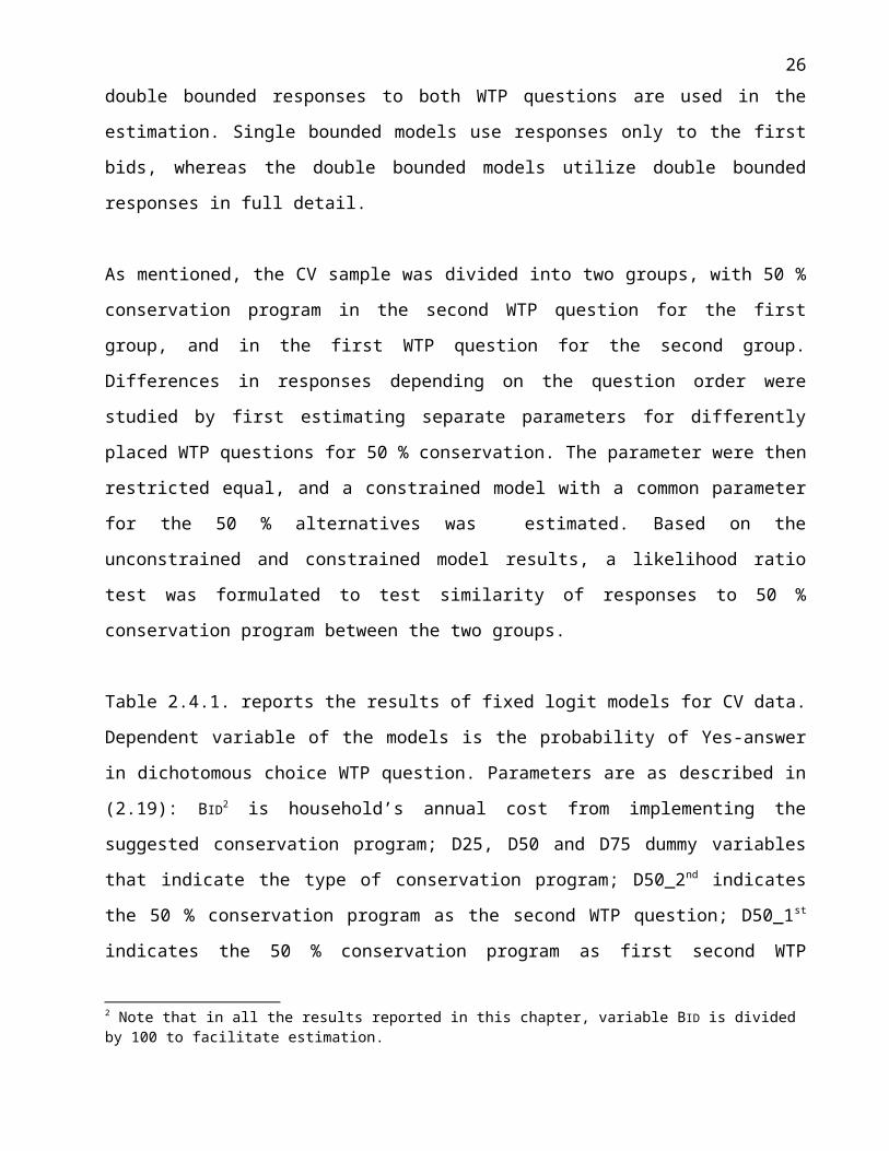
The CV data was used in estimating both single and double bounded models. The data with 376

observations was first censored for missing responses. The remining 306 observations with

complete double bounded responses to both WTP questions are used in the estimation. Single

bounded models use responses only to the first bids, whereas the double bounded models utilize

double bounded responses in full detail.

As mentioned, the CV sample was divided into two groups, with 50 % conservation program in the

second WTP question for the first group, and in the first WTP question for the second group.

Differences in responses depending on the question order were studied by first estimating separate

parameters for differently placed WTP questions for 50 % conservation. The parameter were then

restricted equal, and a constrained model with a common parameter for the 50 % alternatives was

estimated. Based on the unconstrained and constrained model results, a likelihood ratio test was

formulated to test similarity of responses to 50 % conservation program between the two groups.

Table 2.4.1. reports the results of fixed logit models for CV data. Dependent variable of the models

is the probability of Yes-answer in dichotomous choice WTP question. Parameters are as described

in (2.19): BID2 is household’s annual cost from implementing the suggested conservation program;

D25, D50 and D75 dummy variables that indicate the type of conservation program; D50_2nd

indicates the 50 % conservation program as the second WTP question; D50_1st indicates the 50 %

conservation program as first second WTP question; D50 is a dummy that pools 50 % conservation

programs by restricting D50_2nd = D50_1st.

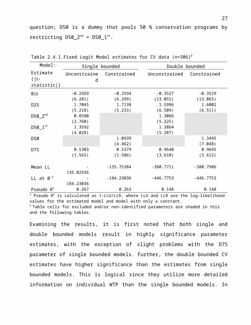
Table 2.4.1.Fixed Logit Model estimates for CV data (n=306)b

Model: Single bounded Double bounded

2 Note that in all the results reported in this chapter, variable BID is divided by 100 to facilitate estimation.

16

Estimate(|t-statistic|)

Unconstrained Constrained Unconstrained Constrained

BID -0.2569(6.281)

-0.2594(6.299)

-0.3527(13.055)

-0.3529(13.065)

D25 1.7045(5.218)

1.7138(5.233)

1.5996(6.509)

1.6002(6.511)

D50_2nd 0.8580(2.760)

1.3066(5.225)

D50_1st 1.3592(4.028)

1.3864(5.287)

D50 1.0939(4.462)

1.3445(7.048)

D75 0.5303(1.565)

0.5379(1.586)

0.9640(3.610)

0.9645(3.612)

Mean LL -135.02556 -135.75384 -380.7711 -380.7986LL at 0 a -184.23036 -184.23036 -446.7753 -446.7753Pseudo R2 0.267 0.263 0.148 0.148

a Pseudo R2 is calculated as 1-LLU/LLR, where LLU and LLR are the log-likelihood values for the estimated model and model with only a constant. b Table cells for excluded and/or non-identified parameters are shaded in this and the following tables.

Examining the results, it is first noted that both single and double bounded models result in highly

significance parameter estimates, with the exception of slight problems with the D75 parameter of

single bounded models. Further, the double bounded CV estimates have higher significance than the

estimates from single bounded models. This is logical since they utilize more detailed information

on individual WTP than the single bounded models. In terms of explanatory power of the models,

single bounded models perform well in relation to the double bounded models. The pseudo-R2

measure for single bounded models (0.263 – 0.268) is almost twice the pseudo-R2 for double

bounded models (0.148 – 0.148). This is likely to have resulted from more response variation in

second than first responses, causing the double bounded models to explain less of the total variation

in the estimated model.

Examining policy alternative dummies is interesting. The estimate for D25 is big and significantly

greater than zero, suggesting that the 25 % conservation program is preferred to status quo. The

estimates for D50 and D75 are positive and generally greater than zero. Therefore, they are also

preferred to status quo. However, the estimate for D50 is systematically lower than the estimate for

D25, and the estimate of D75 in turn lower than the one for D50. This suggests a conservation

policy preference order (D25 > D50 > D75 > status quo), with increasing WTP for implementing 25

% conservation, with a possibly negative marginal WTP for higher levels of conservation.

17

No statistically significant differences for responses to 50 % conservation program can be found on

the values of maximized log-likelihood functions. The likelihood ratio test statistic3 between the

unconstrained and constrained models is 1.45 for the single bounded model, and 0.05 for the double

bounded model. The LR tests reject the null hypothesis of different parameter estimates for D50_1st

and D50_2nd, and suggest accepting a constrained model. Based on strong rejection of the null

hypotheses, constrained models are used in further analysis of the CV data. In practical terms, this

means that data on responses to 50 % conservation program are from now on pooled and D50

estimated using a single parameter.

Contingent Rating/Ranking

All the models for CR data are based on rankings that were obtained by transforming respondents’

ratings for policy alternatives into a preference order, assuming that preferred alternatives are rated

higher than the less preferred ones. Rankings utilize only ordered information on preferences.

Respondents with ratings sequences (3,2,1,0) and (10,9,3,1) are therefore considered similar

responses with the same preference ordering A>B>C>D. In building the ranking data, observations

with tied or missing ratings were censored, leaving a total of 270 observation left for the estimation.

The results are therefore based on data with full and unique rankings of all four policy alternatives.

Model specification for the CR data is the same as for the CV data. The following models were

estimated: (1) conditional logit model for highest ranked alternative out of all the alternatives i.e.

conditional logit model for preferred choice, (2) rank-ordered logit models for two and three ranks,

both as rank-homoscedastic (ROL) and rank-heteroscedastic models (HROL).

Several rank-ordered logit models were estimated in order to examine consistency of rankings.

Information on more than only the preferred alternative is of course valuable, but beneficial only if

rankings are consistent and generated by same parameters. It is known from empirical applications

that the variance of stochastic term in RU model tends to change (typically increase) as the ranking

is continued. This has been suggested to result from people ranking the preferred alternatives with

more care than the less preferred alternatives, causing data on 2nd ranks to be more noisy than data

on 1st rank, data on 3rd rank to be more noisy than data on 2nd rank, and so forth.

3 LR-test statistic is calculated as –2(LLR-LLU), where LLR and LLU are the values of maximized log- likelihood function for constrained and unconstrained models, respectively (e.g. Amemiya 1983).

18

Changing variance of random term between the ranks violates the i.i.d. assumption of rank-ordered

logit model. Inconsistent rankings reveal violations of this assumption. Models with violations

should be rejected and models for fewer ranks used instead. If variance of the random term changes

sufficiently systematically and similarly over the rankings, problem could be solved by applying a

Hausman –Ruud rank-heteroscedastic logit model. Testing the consistency of for instance first and

second ranks, the unconstrained log-likelihood value can be obtained as a sum LL1 + LL2, where

LL1 and LL2 are values of maximized log-likelihood function of separate conditional logit models

for first and second rank. Constrained model is then estimated as a rank-ordered logit model for two

ranks, resulting a maximized log-likelihood value LLR. LR-test statistic with degrees of freedom

equal to number of constrained parameters is calculated as –2*(LLR-LL1+LL2). If LR-test statistic

is insignificant, ranks can be pooled and a rank-ordered logit model for two ranks used. If LR-test

fails to accept pooling of ranks, a Hausman-Ruud style rank-heteroscedastic logit model can be

estimated and similar LR-test procedure carried out with it, this time with one less degrees of

freedom because an additional parameter is estimated.

Table 2.4.2. reports the results of fixed parameter CR models. The signs, relative magnitudes and

statistical significances of parameter estimates are rather well in line with the estimates of the CV

models. In particular, parameter estimate for D25 is always greater than estimates for parameters

D50 and D75. The CR models suggest also uniformly that in the average, the 25 % conservation

policy alternative is preferred over all the other policy alternatives, including status quo. Moreover,

the relation between parameters D50 and D75 is similar as in the CV results, with D75 having the

smallest absolute but still a positive estimate.

In comparison to the CV results, the main overall difference is the uniform insignificance of

estimate for D75 in all the CR models. This can be related to questionnaire design; the policy

alternative with 75 % conservation was presented always as the last policy alternative, which could

have resulted in less carefull rating than was the case with first, second and third alternative.

Another possible explanation is that preferences regarding the 75 % conservation policy are simply

so heterogeneous that the identification of parameters is difficult.

Table 2.4.2. Fixed logit models for contingent rating/ranking data (n=270)

Model: 1 Rank 2 Ranks 3 Ranks

19

Estimate (|t-statistic|)

ROL HROL ROL HROLb

BID -0.0888(-3.153)

-0.0779(-3.904)

-0.0484(-2.275)

-0.0592(-3.635)

-0.00099(-1.340)

D25 0.3537(1.328)

0.7561(3.783)

0.6217(3.321)

1.1588(6.282)

0.4519(2.083)

D50 0.2760(0.818)

0.5559(2.242)

0.4358(2.226)

0.9959(4.522)

0.3445(2.000)

D75 0.2055(0.507)

0.1155(0.368)

0.0672(0.297)

0.1473(0.531)

0.0480(0.578)

Rank2,3 1.8146(2.765)

4.6160(1.980)

LL -150.709 -261.938 -260.515 -319.496 -307.919

LL at zero -162.556 -291.379 -291.379 -372.657 -372.657

Pseudo R2a 0.073 0.101 0.106 0.143 0.174a Pseudo R2 is calculated as 1-LLU/LLR, where LLU and LLR are the log-likelihood values for the estimated model and model with all the parameters constrained equal to zero.b Hausman-Ruud rank-heteroskedastic model for three ranks is estimated with common scale factor for the second and third rank. Estimating separate scale factors for second and third ranks is structurally possible but they could not be identified.

Conditional logit model for first rank results in low statistical significances of estimates, with all the

parameters except for BID statistically insignificant. In addition to noisy data, this can be related to

relatively small number of observations.

Examining next the homoscedastic rank ordered logit models, it is noted that all the statistically

significant parameter estimates are greater in the absolute magnitude than their counterparts in the

first rank model. This is a logical, since by utilizing more information on individual preferences, the

relative magnitude of stochastic term in the RUM is decreased and substituted by higher parameter

estimates and therefore higher proportion of observed variation. Further, all the parameter estimates

except D75 are now statiscally significant both in two and three rank models. The pseudo R2

measures are still relatively low, but improved from the first rank model.

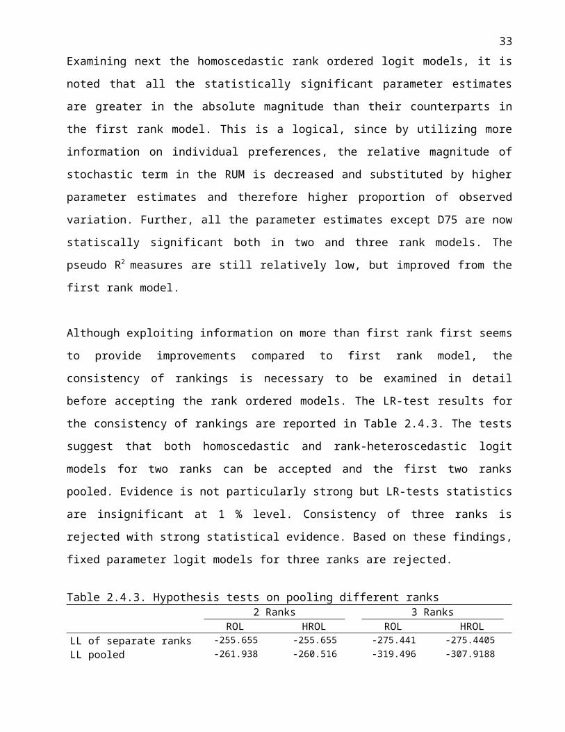
Although exploiting information on more than first rank first seems to provide improvements

compared to first rank model, the consistency of rankings is necessary to be examined in detail

before accepting the rank ordered models. The LR-test results for the consistency of rankings are

reported in Table 2.4.3. The tests suggest that both homoscedastic and rank-heteroscedastic logit

20

models for two ranks can be accepted and the first two ranks pooled. Evidence is not particularly

strong but LR-tests statistics are insignificant at 1 % level. Consistency of three ranks is rejected

with strong statistical evidence. Based on these findings, fixed parameter logit models for three

ranks are rejected.

Table 2.4.3. Hypothesis tests on pooling different ranks2 Ranks 3 Ranks

ROL HROL ROL HROLLL of separate ranks -255.655 -255.655 -275.441 -275.4405LL pooled -261.938 -260.516 -319.496 -307.91882 (H0 vs. H1)a 12.57 9.72 88.11 64.95Pooling of ranks Accepted Accepted Rejected Rejected

a At 1 % significance level, critical values for 2 test statistic for 3 and 4 degrees of freedom are 11.34 and 13.28, respectively

Table 2.4.2. also reports the results of Hausman-Ruud style rank-heteroscedastic logit models

(HROL). They are obtained by fixing the scale factor for first rank and estimating relative scale

factors for second and third ranks. In both HROL models, estimates of scale factors are significantly

greater than one. Being inversely related to the magnitude of random term in the RU model, this

suggest that magnitude of random term decreases as ranks are added. Results from consistency tests

suggest that heterogeneity of responses is not related to ranking tasks.

21

2.4.2. Random Parameter Logit Models

At least two important aspects of modeling strategy must be considered carefully before estimating

random parameter models. First, parameters with and without heterogeneity must be selected using

prior information or some other criteria. Second, distributions for random coefficients must be

specified, typically based on theoretical considerations.

In selecting heterogeneous and homogeneous coefficients, it is of course possible to allow all the

parameters to vary in population. This strategy relies on flexible specification that lets the results

suggest which parameters vary in population and which do not. Before following this approach, it

should supported by expectations about parameter heterogeneity. Not only the evident

methodological but also time considerations suggest that. Even with given recent improvements in

computing power, estimating random parameter models can be very time consuming4. For instance,

the speed of Train’s simulator mainly depends on the number of estimated heterogeneous

parameters, and inclusion of irrelevant heterogeneous parameters should be avoided. Further,

identification is always an issue in estimating random parameters, especially with

non-negative/positive coefficients. As it only gets harder with increasing number of random

parameters, careful selection of heterogeneous parameters is recommend.

Typically, random parameters are estimated as normally distributed parameters. Normally

distributed parameters n can get both negative and positive values, and they are estimated by

expressing them as n=(bn +ne), where b and are estimated mean and deviation parameters of n,

and e a standard normal deviate (Train 1998).

Economic theory, as well as common sense often suggests that some random coefficients of SP

models should be non-negatively/positively distributed. Here such an example is coefficient BID

that is expected to be non-positive. This is justified by logic that increasing the costs of a policy

alternative should not increase its probability to become chosen but the opposite.

4 For instance, many of the models reported in this chapter took more than half a day to converge with an up-to-date processor. In addition, several runs with different starting values are often needed to find the global maximum, since the log-likelihood functions of the RP models, unlike their fixed parameter counterparts, are not necessarily globally convex and can therefore have multiple local maximum (McFadden & Train 2000).

22

Train (1998) suggests non-positive/negative random parameters to be estimated log-normally

distributed, and provides a practical method for incorporating that into his simulator. Each log-

normal k can be estimated by expressing them as k=exp(bk+ke), where b and are estimated

mean and deviation parameters of ln(k), and e an independent standard normal deviate. Log-normal

non-positive parameters are estimated with entering the appropriate exogenous variables as their

negative. For disadvantage of models with log-normally distributed random parameters, they are

often very hard to estimate and to identify (e.g. McFadden and Train 2000).

Alternatively, Layton (2000b) proposes employing distributions determined by a single parameter

in estimating non-negative/positive random parameters. While RP models typically estimate mean

and variance of the RP distribution, one-parameter- distributions (such as Rayleigh-distribution)

allow finding all the moments of RP distribution by estimating a single parameter. A non-negative

parameter x with Rayleigh distribution has a cumulative density function F(x)=1-exp[-x2/(2b2)] and

a probability density function f(x)=(x/b2)exp[-x2/(2b2)], where b is the scale parameter fully

determining the shape of distribution. Using an inverse transformation method, Rayleigh distributed

x can be obtained as x = (-2b2ln(1-u))1/2, where u is a random uniform deviate and b the estimated

scale factor. The mean, variance, median and mode of Rayleigh-distributed x are b(/2)½, (2-

/2)b2, b(log4), and b, respectively (Layton 2000b).

In the case at hand, both BID and policy alternative dummies were modeled as random parameters.

Most available RP applications have modeled either BID or alternative specific dummies as random

parameters, not both. With these data, heterogeneity of preferences for policy alternatives with

extensive conservation levels was likely to appear, and random parameter formulation of policy

alternative dummies is therefore of specific interest. On the other hand, previous studies suggest

that heterogeneity of preferences is often related to BID coefficient, that is therefore also estimated

as a random parameter. Since it essentially represents the negative of marginal utility of income, it

was estimated as a non-positively distributed parameter. Despite continuous and substantial efforts,

all the necessary models for this study were impossible to be estimated with log-normal BID5. BID

5 The estimation of CV models with log-normally distributed BID was generally more successful, although excessively time consuming. The estimation of CR models did not succeed. Especially with models for more than one rank, iteration first proceeded seemingly fine for some 80 iterations but failed to convergence. This could be due to multiple local maxima of the log-likelihood function. However, even specifications with BID as a sole random parameter did not lead to convergence of the models.

23

was therefore expressed as a Rayleigh-distributed random parameter BID – RAYLEIGH6. With this

specification, convergence was reached much easier and estimation considerably speeded up.

Table 2.4.4. Random coefficient logit models for CV (n=306) and CR data (n = 270) a

Model: DB CVb1 Rankc 2 Ranksd 3 Ranksd

Estimate (t-statistic)

Random dummies

Fixed dummies

Fixed dummies

Random dummies

Fixed dummies

Random dummies

BIDRAYLEIGH 1.1309(3.014)

0.0760(2.606)

-0.1094(3.315)

0.1257(2.396)

-0.1672 (3.395)

0.1578(3.116)

D25-mean 3.6657(2.905)

0.3879(1.393)

0.9261(4.059)

1.1133(3.506)

1.5260(6.522)

1.7359(5.742)

D50-mean 3.5006(2.882)

0.2965(0.828)

0.8975(2.919)

0.8660(1.422)

1.7305(5.398)

1.4423(2.313

D75-mean 3.1339(2.779)

0.1961(0.458)

0.5156(1.359)

-1.8904(1.332)

1.1550(2.860)

-0.2733(0.281)

D25-deviation -1.6448(1.304)

0.0122(0.022)

0.0349(0.043)

D50-deviation 1.5736(1.290)

3.3713(4.650)

3.6318(5.251)

D75-deviation 1.7742(1.417)

6.2289(4.130)

5.7319(5.754)

LL -333.18 -151.11 -258.87 -224.04 -309.987 -262.19

LL at zero -446.78 -162.56 -291.38 -291.38 -372.66 -372.66

Pseudo R2 0.254 0.0704 0.112 0.231 0.168 0.296a A simulator with 200 draws were used in estimating all the models. b Model results for DB CV with fixed and random normal dummies are similar and not statistically significantly different. Results with fixed dummies are not presented here for clarity of presentation. Specification with random normal dummies is chosen for CV data to make results directly comparable to CR, necessary for data pooling purposes that is reported in the next section of the paper. c Deviations cannot be identified in the model for the first rank, and the results for it are therefore based on model that restricts them as zero. d Hausman and Ruud rank heteroscedastic model cannot be identied for CV and CR data on two or three ranks.

Table 2.4.4. reports random parameter model results for both CV and CR data. Results with both

fixed and random policy alternative dummies are reported for CR models for two and three ranks to

demonstrate importance dummy parameter heterogeneity in them. Pseudo-R2 of CR models for 2

and 3 ranks increased from 0.106 and 0.143 of fixed logit models to 0.231 and 0.296. Therefore, the

explanatory power of the models more than doubled as a result of incorporating unobserved

preference heterogeneity. Significant portion of the improvement is gained by inclusion of random

6 Dave Layton is acknowledged for suggesting this.

24

normal dummies, as can be seen from pseudo-R2 measures for two and three rank CR models with

and without random dummies.

Heterogeneity of dummy parameters is less clear in other estimated models. CR model for first rank

does not converge with random dummies and its results cannot be reported; a model with fixed

dummies and random bid parameter is reported instead. The CR model for first rank performs

poorly also in terms of explanatory power. In the double bounded CV model, policy alternative

dummies are not significant. In addition to true insignificance of deviation estimates for dummies,

insignificance could have resulted from using a relatively modest number of draws in simulation.

Explanatory power of the CV models is increased substantially; pseudo R2 of the double bounded

CV model increased from 0.148 to 0.267.

Estimates of deviations for D50 and D75 (D50–deviation, D75-deviation) are strikingly large and

significant, suggesting that preference heterogeneity for policy alternatives is considerable and

should be taken into account while modeling these data. Parameter heterogeneity is also one

possible explanation for insignificance of the mean estimates of D75 in these models. With highly

variable preferences for 75 % policy alternative, estimation cannot provide a significant estimate of

the location parameter for distribution of D75. Note that the same phenomena was observed in fixed

parameter logit models, where significance of D75 estimate was lower than in these RP models.

Random parameter formulation provides estimation of both CV and CR data with significant

improvements. They are next applied together with fixed parameter logit models to combined CV

and CR data that estimate pooled models for the CV and CR data.

25

2.4.3. Pooled models for CV and CR data

Pooled models are estimated using combined CV and CR data. Estimation can be implemented in

several ways; main concern is to make sure appropriate likelihood functions are applied to each

respondent. An indicator variable for CR data can facilitate estimation. Defining IiCR with a value 1

for respondents with CR questionnaire and value 0 for CV respondents, the pooled log-likelihood

function for individual i is determined as LLi= IiCR*PiCR + (1- IiCR)*PiiCV, where PiCRand PiCV are the

appropriate response CV and CR probabilities of the model. Similarly as with unpooled models, the

pooled total log-likelihood function is a sum of individual likelihoods over the whole sample7.

Table 2.4.5. reports the models results for combined CV and CR data. A variety of pooled models

were estimated to examine the effects of modeling choices on accepting/rejecting pooling the data.

The same specification as in unpooled models was applied for pooled models. Unpooled

counterparts of all the pooled models can be found from previous sections. LR-tests are used for

accepting/rejecting the pooling hypothesis, and the respective LR-test statistics are reported in the

second last row of Table 2.4.5. Test statistics follow 2 distribution with degrees of freedom equal to

difference in number of estimated parameters between pooled and unpooled models. Estimating a

scale parameter in pooled model versions, degrees of freedom for fixed and random parameter logit

models with all parameter random equal to 3 and 6, respectively. The respective critical values are

11.34 and 18.48. LR-test statistics for random parameter models with random BID and fixed policy

alternative dummies also have 3 degrees of freedom. If LR-test statistic is smaller than the critical

value, pooling of data cannot be rejected.

All the reported model results include an estimate for parameter CR. It is a scale factor for CR data,

accounting for possible differences in the variance of random term of RU model between CV and

CR data. As noted before, only parameter relations are comparable between different sources of

data. Estimating a scale factor as part of the model allows for direct comparisons of parameter

estimates. Logically, if no differences in random term variance exist between the CV and CR data,

estimate of CR is not statistically different from one. Since scale factor is inversely related to the

7 Considerable time savings, especially in estimating random parameter models, can be obtained by structuring the program so that unnecessary calculations are avoided in calculating the log-likelihood function. Calculations of CR response probabilities are uncessary for CV respondents, vice versa.

26

variance of random component of the RU-model, an estimate CR < 1 suggests that CR data consists

of noisier observations than the CV data, and CR >1 the opposite.

First model pools fixed parameter versions of single bounded CV modeland a CR model for first

rank. These two models use data in least detail and can be assumed to among the most likely models

to provide support for accepting pooling the CV and CR data, if accepted by any models. Results of

“SB CV & 1 Rank” model confirm this. Maximized log-likelihood value of pooled model is almost

the same as for the unpooled model, resulting in LR-test statistic of 0.44. The model also results in

substantially high pseudo-R2 (0.33), and strongly significant estimates with expected signs. Estimate

of CR is 0.3044, statistically significant and substantially smaller than one.

Models “DB CV & 1 Rank” pool double bounded CV model with a CR model for first rank, using

both fixed (FL) and random coefficient (RCL) formulation. Both FL and RCL model results provide

relatively strong support for accepting the pooling hypothesis. Estimates of CR are statistically

significant and smaller than one in both models. Random parameter model provides a significantly

higher explanatory power than the fixed parameter counterpart.

“DB CV & 2 Rank” models pool fixed and random parameter model for double bounded CV and a

CR model for two ranks. Similarly as the previous pooled models, these models result in higly

significant estimated with exptected signs. Comparing unpooled and unpooled fixed parameter

models results in LR-test statistic 6.3 and acceptance of pooling the data. However, the pooled

random parameter model clearly rejects pooling of CV and CR data. Despite rejection of pooling,

the random parameter model results in substantially higher pseudo-R2 than the fixed parameter

model.

Models “DB CV & 3 Rank” pool fixed and random parameter model for three ranks and double

bounded CV. Results from these models are similar with pooled models with CR model for two

ranks. However, pooling of CV and CR data is now strongly rejected for both fixed and random

parameter models. Stronger rejection of pooling with the random parameter models, together with

results of pooled models with CR model for two ranks, suggest that differences in parameter

heterogeneity between the two data are a possible source of rejecting the pooling hypothesis with

relatively detailed models such as a CR model for two ranks.

27

Table 2.4.5. Logit Models for Pooled CV and CR Data (n=576)

Model: SB CV & DB CV & DB CV & DB CV &

Estimate (t-statistic)

1 Rank 1 Rank 2 Rank 3 Rank

FL FL RCLa FL RCLb FL RCLb

Bid – Fixed -0.2645(6.445)

-0.3532(13.077)

-0.3484(12.963)

-0.3402(12.677)

Bid-Rayleigh 0.8516 (6.351)

1.1286(2.994)

0.8380(3.123)

D25 – mean 1.6484(5.160)

1.5928 (6.669)

2.7152 (7.684)

1.7335 (7.436)

3.7174(2.876)

1.8513(7.961)

3.1829(3.094)

D50 – mean 1.1107(4.589)

1.3410 (7.120)

2.5373 (8.015)

1.3727(7.398)

3.5140 (2.853)

1.4679(7.985)

3.7130(3.409)

D75 – mean 0.5777(1.772)

0.9672 (3.697)

2.2661 (5.545)

0.8606(3.373)

3.1244 (2.757)

0.7131(2.848)

3.3504(3.128)

D25 – dev -1.6906 (1.326)

-0.8670 (0.738)

D50 – dev 1.6001 (1.297)

2.6625(2.564)

D75 – dev 1.7806 (1.414)

4.2451(2.925)

CR 0.3044(3.389)

0.2549 (3.781)

0.0905 (2.902)

0.2617(5.395)

0.0688 (2.218)

0.2490(5.996)

0.9103(3.747)

LL pooled -286.90 531.54 485.43 -645.89 613.33 -719.34 -633.91

LL unpooled -286.46 531.50 485.19 -642.74 595.11 -700.30 -595.37

LL at zero 428.06 609.33 609.33 738.15 738.15 819.432 819.432

LR-test of pooling

0.44 0.063 0.5 6.3 36.45 38.08 77.08

Pseudo R2 0.330 0.128 0.203 0.125 0.169 0.122 0.226a Since the CR model for 1 rank with random dummies could not be estimated, a pooled model for DB CV and 1 Rank CR is also based on model with fixed dummies and Rayleigh bidb Hausman and Ruud heteroscedastic logit model is not identied for CV and CR data on two or three ranks.

Similarity of parameter estimates accross all the models is a distinctive feature of the pooled model

results. This is likely to have resulted from more precise estimates of CV models data “dominating”

the identification of estimates for the pooled models. With lower variability of the random term of

RUM, as suggested by estimates of CR being uniformly less than one, CV data plays a relatively

more important role in finding the estimates, even with almost equal number of CV and CR

observations.

28

Although not reported in Table 2.4.5., pooling of data was further tested with restriction CR=1 that

imposes equality of the variance of RUM random terms between CV and CV models. Using this

fully pooled model, pooling of CV and CR data is rejected using all the models. The most likely

candidate providing support for complete invariance hypothesis is the pooled model for DB CV and

first rank CR data, since it provides the strongest support for accepting pooling with an estimated

CR scale factor. Using this model, LR test for pooling results in value 45.5, strongly rejecting

complete pooling of CV and CR data. Other models are less likely to provide support for complete

pooling hypothesis, and complete invariance of CV and CR data is therefore uniformly rejected.

2.5. Willingness to Pay Estimates

Inclusion of policy implementation costs and policy specific dummies in estimated models allows

capturing WTP for different policy scenarios indirectly from the results. The mean WTP for policy

alternative xj is calculated as (e.g. Goett et al. 2000)

(2.21)

In the reported results, is measured by alternative specific dummies as D25, D50 and D75,

and by BID estimate. Mean WTP estimates for fixed logit estimates are calculated as

D25/BID, D50/BID and D75/BID. Means of normally distributed random parameters equal their

estimates and calculation of WTP is similar as with the fixed parameter models. In the case of

random parameter with non-negative/positive distributions such as Rayleigh or log-normal

distribution, the mean estimates for parameters must be first calculated.

Table 2.4.6 reports the mean WTP estimates for different estimated models. Results are divided into

fixed and random parameter models for unpooled and pooled data. In the previous analyses, the

following models were clearly rejected because of inconsistency of rankings or failure to accept

data pooling hypothesis: (a) Fixed logit model “CR-3 rank data” for three ranks in CR data, (b)

Pooled fixed logit model “CV DB & CR – 3 rank” for pooled double bounded CV and three rank

CR data, (c) pooled random parameter model “CV DB & CR-2 rank” and (d) pooled random

parameter model “CV DB & CR-3 rank”. Their results are shown in the Table 2.4.6. in comparison

with other models.

29

Table 2.4.6. Willingness to pay estimates (USD) a, b

Policy

Model type alternative CV SB CV DB CRM - 1 Rank CRM - 2 Rank CRM - 3 Rank

Fixed logit 25 % 107 73 - 156 315

50 % 68 61 - 115 271

75 % 33 44 - - -

Random logit 25 % - 42 - 95 142

50 % - 40 - 92 118

75 % - 36 - 53 -

Pooled models CV SB +CR – 1 rank

CV DB +CR – 1 rank

CV DB +CR – 2 rank

CV DB +CR – 3 rank

Fixed logit 25 % 100 73 80 88

50 % 68 61 64 70

75 % 35 44 40 34

Random logit 25 % - 41 42 49

50 % - 38 40 57

75 % - 34 34 51a Insignificant estimates are expressed with NAb USD=FIM 6.2

Results for 75 % conservation alternative are strikingly similar across all the models providing it

with a significant estimate. Its WTP vary between 207 and 327. Variation in WTP estimates for 50

% cover a considerable wider range from 238 and 729, similarly as WTP for 25 % conservation

alternatives that gets values 254 and 970 .

All the significant and accepted WTP models result consistently higher WTP for 25 % alternative

than for 50 % alternative, and in turn for higher WTP for 50 % alternative than for 75 % alternative.

There is a clear tendency for random parameter models to result in lower WTP estimates than their

fixed parameter counterparts. This is possibly due to their ability to better account for observations

with very low and high WTP. Fixed logit models tend to be more sensitive to observations in tails

of the WTP distribution.

30

2.6. Discussion

This study examined different econometric modeling strategies for CV and CR survey data. Both

conventional fixed logit models and recently developed random parameter logit models were

reviewed and applied to the data at hand. The results provided another confirmation that

considerable care must be practised in applying fixed parameter logit models. Especially the fixed

parameter models for the CR data on full rankings of four alternatives violated assumptions of

conditinal logit model. Their results differed by an order of magnitude from the results of consistent

models.

Applying data pooling techniques in testing for equality between CV and CR was the second

primary objective of this study. Succesful pooling of data required use of response probability

models with minimal differences between CV and CR data, and estimation of scale factors for

separate data sources. The scale factors make parameter estimates comparable accross separate

sources of data. With scale factors in the estimated model, pooling of CV and CR data could not be

uniformly rejected or accepted. The more detailed models for CV and CR responses are likely to

reject the pooling hypothesis. Less detailed models such as single bounded CV and conditional

choice logit models generally did not provide sufficient statistical evidence for rejecting the pooling

hypothesis.

Applying random parameter models does not seem to provide a miracle in terms of solving

differences between CV and CR data, although there is some evidence that fixed logit models could

exaggerate the differences between WTP results for CV and CR data. Especially the results of the

rejected fixed logit models for three ranks CR data suggest that.

Data pooling techiques provide a powerful apprach to tests for invariance between different sources

of data. The analysis of pooled data that has been presented in this paper highlights only some of the

possible uses of data pooling methods in examining SP survey methdos. For instance, sources of

differences between different SP sources can be further examined using the same framework.

Issue of negative marginal WTP for conservation after reaching a certain conservation levels, is of

course very interesting and worth some further investigation. Given relatively critical views of some

31

of the public for increasing the forest conservation in Finland, the result is not necessarily a

surprising finding. Most Finns probably agree with moderate increases in conservation, but are

reluctant to show support to extensive conservation programs that they often view as regulatory

“overshootings”.

Precision of WTP estimates has not been considered in this analysis yet. Use of random parameter

models, as well as pooling different sources of SP data, could provide more precise WTP estimates

than conventionally used fixed parameter models. This remains an issue for immediate further

investigation.

32

References

Adamoviz, W., Louviere, J. & Williams, M. 1994. Combining revealed and stated preference methods for valuing environmental amenities. Journal of Environmental Economics and Management 26:271-292.

Amemiya, T. 1985. Advanced Econometrics. Harvard University Press. 521 p.

Beggs, S., Cardell, S. & Hausman, J. 1981. Assessing the potential demand for electric cars. Journal of Econometrics 16:1-19.

Bishop, R. C. & Heberlein, T. A. 1979. Measuring Values of Extramarket Goods: Are Indirect Measured Biased? American Journal of Agricultural Economics 926:929.

Boxall, P., Adamoviz, W., Swait, J., Williams, M. & Louviere, J.1996. A comparison of stated preference methods for environmental valuation. Ecological Economics 18:243-253.

Brownstone, D. & Train, K. 1999. Forecasting New Product Penetration with Flexible Substitution Patterns. Journal of Econometrics, Vol. 89(1):109-129.

Carson, R.T., Louviere,J.J., Anderson, D. A., Arabie, P., Bunch, D.S., Hensher, D. A., Johnson, R.M., Kuhfeld, W.F., Steinberg, D., Swait, J., Timmermans, H. & Wiley, J.B. Experimental Analysis of Choice. Marketing Letters 5:351-368.

Cameron, A.C. & Trivedi.1998. Regression analysis of count data. Econometrci Society Monographs 30.

Chapman, R.G. & Staelin, R. 1982. Exploiting rank ordered choice set data within the stochastic utility model. Journal of Marketing Research 19: 288-301.

Desvouges, W.H. & Smith, V.K. 1983. Option price estimates for water quality improvements: a contingent valuation study for Monogahela river. Journal of Environmental Economics and Management 14:248-267.

Goett, A., Hudson, K. & Train, K. 2000. Customers’ Choice Among Retail Energy Suppliers: The Willigness-to-Pay for Service Attributes. Working paper, Department of Economics, University of California, Berkeley.

Hanemann, M. W. 1984. Welfare Evaluations in Contingent Valuation Experiments with Discrete Responses. American Journal of Agricultural Economics 66:332-341.

Hanemann, M. W., Loomis, J. & Kanninen, B. 1991. Statistical Efficiency of Double-Bounded Dichotomous Choice Contingent Valuation. American Journal of Agricultural Economics 1255:1263.

Hanemann, M.W. & Kanninen, B. The Statistical Analysis of Discrete-Response CV Data. In Valuing Environmental Preferences: Theory and Practice of the Contingent Valuation (ed. Bateman, I & Willis, K.).

33

Hausman, J.A. & Ruud, P.A. 1987. Specifying and testing econometric models for rank-ordered data. Journal of Econometrics 34:83-104.

Hensher, D, Louviere, J.J. & Swait, J. 1999. Combining sources of preference data. Journal of Econometrics 89:197-221.

Layton, D.F. 2000a. Random Coefficient Models for Stated Preference Surveys. Journal of Environmental Economics and Management 40:21-36.

Layton, D.F. 2000b. Notes on One Parameter Family of Distributions for Random Coefficient Models. Department of Environmental Policy and Science. University of California Davis.

Louviere, J.J. & Hensher, D.A. 1983. Using Discrete Choice Models with Experimental Design Data to Forecast Consumer Demand for a Unique Cultural Event. Journal of Consumer Research 10:348-361.

Magat, W.A., Viscusi, W.K., Huber, J. 1988. Paired comparison and contingent valuation approaches to morbidity risk valuation. Journal of Environmental Economics and Management 15:395-411.

McFadden, D.1974. Conditional logit analysis of qualitative choice behavior, in Zarembka, P. (ed.), Frontiers in Econometrics, Academic Press, New York.

McFadden, D. & Train, K. 2000. Mixed MNL Models for Discrete Response. Forthcoming in Journal of Applied Econometrics.

Revelt, D. & Train, K. 1998. Mixed Logit with Repeated Choice: Households’ Choices of Appliance Efficiency Level. The Review of Economics and Statistics. Vol. 80: 647-657.

Roe, B., Boyle, K.,J. & Teisl, M.,F. Using Conjoint Analysis to Derive Estimates of Compensating Variation. Journal of Environmental Economics and Management 31:145-159.

Stevens, T.H., Belkner, R., Dennis, D., Kittredge, D. & Willis, C. 2000. Comparison of contingent valuation and conjoint analysis in ecosystem management. Ecological Economics 32: 63-74.

Swait, J. & Louviere, J.J. 1993. The role of scale parameter in the estimation and use of generalized extreme utility models. Journal of Marketing Research 10:23-45.

Train, K. 1998. Recreation Demand Models with Taste Differences Over People. Land Economics 74(2):230-39.

34

Appendix. Simulated response probabilities and log-likelihood formulas for CR and CV dataModel Response

probabilitySimulated response probability Simulated log-likelihood function

Conditional logit of preferred choice

SPij

Rank-ordered logit

SPir

Single bounded CV

SPyes

SPno

Double bounded CV

SPyes-yes

SPyes-no

SPno-yes

SPno-no

35