Systems of Frequency Curves Generated by Transformations

of Logistic Variables

by

P.R. Tadikamalla, University of Pittsburghand

N.L. Johnson,* University of North Carolina at Chapel Hill

1. Introduction

The systems of distributions (for a random variable Y) defined by

y+o,q,nY (0 < Y) (1.1)

SB: Z = Y + 0 m{Y/(l-Y)}

-1Z = Y + 0 sinh Y

(0 < Y < 1) (1. 2)

(1. 3)

with 6 > 0, and Z a unit normal variable, have been described by Johnson

(1949); and with Z a standard Laplace (double exponential) variable, (Si, 58'5U) hy Johnson (1954). In the present paper we study analogous systems,

generated by ascribing to Z a standard logistic distribution with probability

density function (pdf)

Z Z -2fZ(z) = e (1 + e )

or, equivalently, with cumulative distribution function (cdf)

-z -1FZ(z) = (1 + e) .

The percentile function (inverse of cdf) is

(1. 4)

(1. 5)

*Research of this author was supported by the Army Research Office unde~ ContractDAAG29-77-C-0035.

2

(1. 6)

We will denote these new systems of distributions by LL' LB, LU according

as transformations (1.1), (1.2), (1.3), respectively, are used. In view of the

cLseness of the shapes of the logistic and normal distributions, it is to be

expected tilat the new systems will exhibit 'some similarity in shape to Sv SB'

and SUo

In fact since (Johnson and Kotz (1970), p.6)

I(I + ('xp(-TIxI13) }-l - ¢(l~~) I < 0.01 for all x (1.7a)

where <1>(11)

parameters y, 8 and

i~ry, liJ8, where

the difference between the cdf of SL B U with, ,"L B U (with the same values of E;, and ;\) with parameters, ,

TIIjJ = -

131516 T 1.7 (1.7b)

cannot exceed 0.01. Although this gives good agreement in the central part of

the distribution, there can be gross disparities in percentile points in the

ta i1 s.

If an S curve and an L curve are fitted using the same first four moments,

we do not find that (i) the ratios (LiS) for y values and for 8 values will each

be about 1. 7, and (ii) the values of E;, and ;\ will be the same. Section 5.4

(Table 4) contains an example wherein this is clearly illustrated. There can be

very considerable disparity between the percentiles in the tails of the distribu-

tions even though (1.7a) is valid.

TIle very simple formula (1.6) for z in terms of FZ(Z) is an obvious practical

advantage of the new systems. Percentile points of fitted distributions can be

obtained very simply.

3

~ 2. The Log-Logistic (LL) Distribution

This distribution has been studied by Shah and Dave (1963). The pdf is

(2.1)

from which it can be seen that it is a special case of Burr's (1942) Type XII

system of distributions. Dubey (1966) called it the Weibull-exponential distri-

bution, and fitted it to some business failure data presented by Lomax (1954).

The pdf is unimodal. The mode is at y = 0 for 0 ~ 1 (giving a reversed

J-shaped curve); it is at y = e-Y(o-I)/(o+I) if 0 > 1. The cdf is

-Y 0-1Fy(Y) = 1 - (I + e y) (2.2)

and the inverse cdf is

(2.3)

where 1"2 ::: y/o .

From (1.1) and (1.4), the r-th moment of Y about zero is

Putting u z z -1= e (1 + e) so that du/dz =

il~ ::: e-r~ J~ ur/o Cl_u)-r/o du = e-rn B(l+ro- l , 1_ro- l )

-r~= e r8 cosec r8

with 8 ::: TI/o, provided r < O. (If r ~ 0, il~ is infinite.)

In particular

E[Y] = e- n 8 cosec 8

(2.4)

(2.5)

4

anc

Var(Y) -2n 2= e 8 cosec 8 (tan8 - 8) . (2.6)

The r-th central moment, ~ , is a multipler

of exp(-rn), and so the moment-ratios ~r/~~/2 ­

282 = ~4/~2 do not depend on n, but only on 8.

(depending on e, but no t on m~ 3/2

in particul ar d3l = ~3h..l2 and

The (/81,62) points lie on a

line which passes through the 'logistic point' (0,4.2) (corresponding to

e -+ 0 (o-~ (0)). Figure 1 shows that LL ('log-logistic') line, and also the SL

(lognormal) line.

The (~, 82) points for LB

(LU

) distributions lie 'above' ('below') the LL

lin~ in Figure 1. This is analogous to the situation for SB' Su and the lognormal

line.

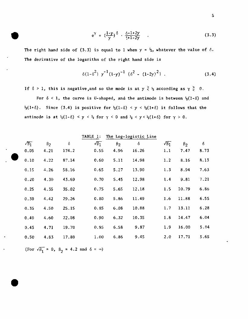
Table 1 gives values of 82 for selected values of 181' for points on the LL

line.

3. The LB System

If transformation (1.2) is valid, with Z standard logistic, then the pdf of

Y is

(0 < y < 1) . (3.1)

If 6 1, we get a 'power function' pdf

(0 < y < 1) . (3.2)

If, in addition, y = 0 we have a standard uniform distribution.

In contrast to the situations when Z has a normal or Laplace distribution,

LB curves cannot be multimodal. There is a single mode (if 6 > 1) or antimode

(if <5 < 1) at the unique value of y between 0 and 1 satisfying the equation

o-1+2y~+1-2y

5

(3.3)

The right hand side of (3.3) is equal to 1 when y = ~, whatever the value of 8.

The derivative of the logarithm of the right hand side is

(3.4)

If 6 > I, this is negative,and so the mode is at y ~ ~ according as y ~ o.

For 0 < I, the curve is U-shaped, and the antimode is between ~(l-o) and

~(1+6). Since (3.4) is positive for ~(l-o) < y < ~(l+o) it follows that the

antimode is at ~(l-6) < y < !:2 for y < 0 and ~ < y < !:2(1+6) for y > o.

TABLE 1: The Log-logistic Line

v'1r1 62 6 IBl 62 6 lSI 62 0

0.05 4.21 174.2 0.55 4.96 16.26 1.1 7.47 8.73

e 0.10 4.22 87.14 0.60 5.11 14.98 1.2 8.16 B.13

0.15 4.26 58.16 0.65 5.27 13.90 1.3 8.94 7.63

0.20 4.30 43.69 0.70 5.45 12.98 1.4 9.81 7.21

0.25 4.35 35.02 0.75 5.65 12.18 1.5 10.79 6.86

0.30 4.42 29.26 0.80 5.86 11.49 1.6 11.88 6.55

0.35 4.50 25.15 0.85 6.08 10.88 1.7 13.11 6.28

0.40 4.60 22.08 0.90 6.32 10.35 1.8 14.47 6.04

0.45 4.71 19.70 0.95 6.58 9.87 1.9 16.00 5.84

0.50 4.83 17.80 1.00 6.86 9.45 2.0 17.71 5.65

(For IBi" = 0, 82 = 4.2 and 6 = (J»)

6

The (~, R2) line corresponding to 0 = 1, which is the 'lower' boundary of the

region with U-shaped curves, is shown in Figure 1. Apart from (3.2), there are

no J - or reverse-J shaped curves in the LB system.

Following an analysis similar to that leading to (2.4) we obtain

(3.5)

with n = y/o, as in Section 2.

Generally, the integral in (3.5) must be evaluated by quadrature. (Of

course, for some special cases - such as 0 = 1 - explicit solutions can be

obtained.) -1 1/0Expansion of the integrand as a power series in (l-u) cannot

be valid over the whole range of integration. Dichotomy of the interval (0,1)

according as (l_u-l)l/o ~ en (i.e. u 5 (l+e-0.)-I) leads to valid expansions ~but the resulting incomplete beta functions must thpmselves (in general) be

evaluated by quadrature.

4. The LV System

If the transformation (1.3) is valid, the pdf of Y is

f (y) ==Y

') 0(y+/(y""+I) )

Y 202{I+e Cy+/(y +1)) }(4.1 )

This curve is unimodal, with mode at the unique value of y satisfying the equation

Y 2 2-Lo{I - e (y + I(y +1)} = y (y +1) '2 (4.2)

Note that, since 0 > 0, the left hand side of (4.2) is a monotonic decreasing

function of y; the right hand side is monotonic increasing.

7

~ The r-th moment of Y about zero is

r= 2- r I

j=Or

= 2- r Ij=O

(-l)j (:) e-(r-2j)~ 1:00

e(r-2j)z/o eZ(l + e z)-2 dzJ

(-l)j (~) e-(r-2j)~ (r-2j)8 cosec(r-2j)8J

(4.3)

provided r < o. If r ~ 6, ~' is infinite. When r = 2j, '0 cosec 0' is inter­r

preted as lim e cosec8 = 1. (As in Section 2, ~ = Y/6 and 8 = TI/6.)8·~

Since (-a)cosec(-a) = acosec a, (4.3) can be simplified.

For r even:

!1r-l~~ = 2-r(_1)~r (~) + 2-(r-1) I (-l)j (~)(r-2j)8 cosec(r-2j)8 cosh(r-2j)~

j=O J (4.4)

For r odd:

-(r-l) ~(r-l) .~' = -2 I (_l)J (~)(r-2j)e cosec(r-2j)8 sinh(r-2j)~

r j=O J

In palticular

~' = -8 cosec 0 sinh ~1

~2 = 8 cosec 28 cosh 2~ - }

~3 = - t 8(cosec 30 sinh 3~ -cosec e sinh m

(4.5)

(4.6)

so that

1~4 = 2 8(cosec 40 cosh 4~ - 2 cosec 28 cosh 2~ )

3+ -8

E[Y] = -8 cosec 8 sinh ~

Var(Y) = ~{(8 cosec 8)2 - l} +2

~ 8 cosec 8(tan8 - 8)cosh 2~

(4.7)

8

5. Fitting the Distributions

5.1. General. The methods of fitting described by Johnson (1949) for the S

systems are also applicable to the L systems, with the advantage that the cdf

of the logistic is simpler than that of the normal distribution.

Introducing the location and scale parameters ~, A respectively, by the

transformation Y = (X-~)/A we obtain a three parameter family for LL:

and four parameter families

z = y + 0 in (X-~) (X > 0 (5.1)

(5.2)

z -1 X-t"Y + 0 £inh (~) (5.3)

f0r LB, LU respectively.

We consider fitting by the methods of moments, percentile points and

maximum likelihood.

Moments. If four parameters are to be fitted, the first four moments of

the distribution of X are equated to those of the fitted curve. It is convenient

to use them in the form of mean (~il' the variance (~2) and the moment ratios

77> 3/2 2 rr;-vB l (= ~3/~2 ) and S2 (= ~4/~2)' Since vSl and 82 are determined by y, 0 and

(fOl' LB and LU' as for SB and SU) conversely, the first step is to determine

Y, ,l) from the specified values of lSI and S2. This could be done using special

tab]es (Table 1,4), or of course a computer program. Once these values are found

the values of ~ and ;\ are determined from the equations

E[X IY, 6] = t, + ;\E [Y IY, 6]

(5.4)

var(Xly, 6) = ;\2 var(Yly, 6)

••

•

••

V-'J r e r::;-Y- .! t:l

e.. Cl €.- k).. ri::~ ':J -/ +} -~3---- -0

'C

••

•

-.,r GJ(~t~~)~ -\ ,,(p..)~) &x C/tl(M+~ ~ ~ ~

~ ~ . I

~ J(~t~ !~) L« J. r~_(~~ :~il-:5(I-\j;tIJ J.rxI~ ~

Jr' '(~ f (IV ') eYx~(L\+~l1:j 11-\ -~-t~Jl ) ,

____ k ~

/\ '

,-

\~[ 1l-~o( \(t-~~-~)~(~",1

---- - ---- e1- ,1-

• -; r~( e" .+:;1-f/] +, ("I e-- (c-'te\:t?( 0 0

- i)

•

••

•

••

y -: .~ tj- M.) .- &-r

"\EL:rC t.(Y;~~ !.~)- fo!<Q\.\-x-~

~~-:I!' ~e&-)( ttj) + JA-

)0'" ,

\[s ( e.<rMe +)A ) - f, ~)]\)/

• ~

;) Lt J ~ fD()..L -+ ~ J

~-A

• r-

•

••

Ie-.u>

•• l-\''; - D

Y", , t,

,~ ((

I 'u(-1>rfI If r f'!

('~f Ii f-.Jr ,,-' I

if"" I H~w/1)

y-, ,L tit- G.(J)F j

• Ie.. I) /1 t,

'~. 1-...\ (\(,t{ ". ~i' 1:- -..:!l. i,\ ..J"

{,. f" \

"" ;}

••

9

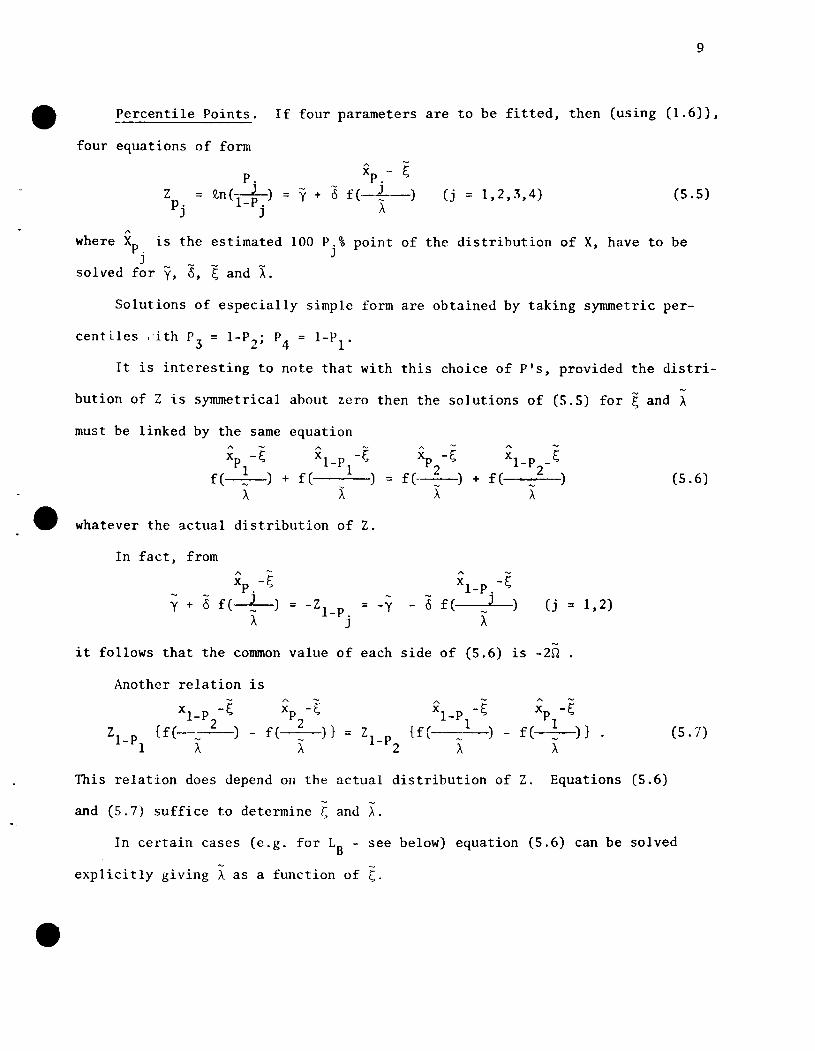
4It Percentile Points. If four parameters are to be fitted, then (using (1.6)),

four equations of form

zp.

J

P.== Q,n(lJ.) == y + 8

J

x - t;P.f( ~ )

A(j == 1,2,3,4) (5.5)

'"where Xp . is theJ

sol ved for y, 8,

estimated 100 P.% point of the distribution of X, have to beJ

~ and X.

Solutions of especially simple form are obtained by taking symmetric per-

centiles .ith P3 == l-P2

; P4

== I-Pl'

It is interesting to note that with this choice of pIS, provided the distri-

bution of Z is symmetrical ahout zero then the solutions of (5.5) for ~ and A

must be linked by the same equation

Xl _P -~

+ f( 1)X

whatever the actual distribution of Z.

In fact, from

x -~P== f( 2 )

,\(5.6)

x -~P.Y + 0 f( ~ )

A== -Z l-P.

J== -y

Xl_P.-~o f( _J )

A(j == 1,2)

it follows that the common value of each side of (5.6) is -2n

Another relation is

xI _P -s xp -~

{f( 2) _ f( 2 )} == Zl_PA A 2

(5.7)

This relation does depend on the actual distribution of Z. Equations (5.6)

and (5.7) suffice to determine [, and A.

In certain cases (e.g. for LB - see below) equation (5.6) can be solved

explicitly giving A as a function of s.

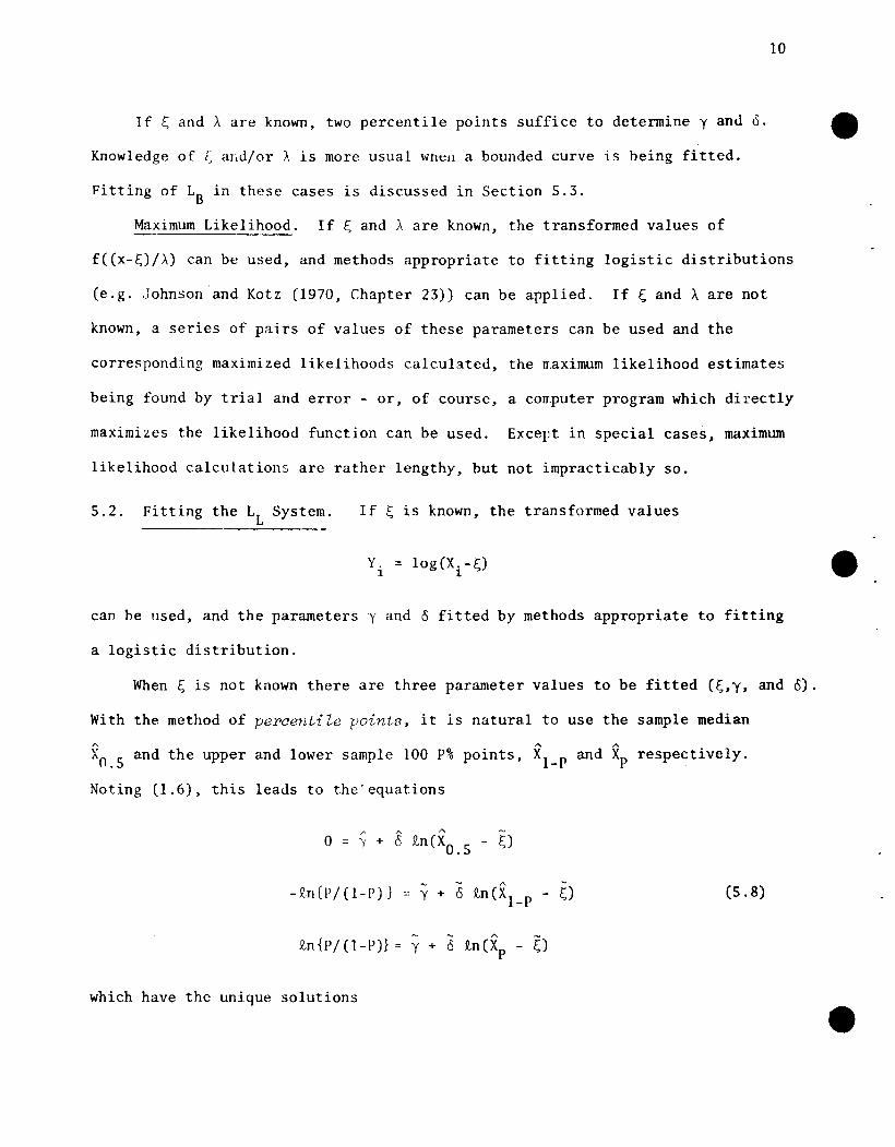
10

If [, and>. are known, two percentile points suffice to determine y and 6.

Knowledge of [, and/or A is more usual \\InCH a bounded curve is being fitted.

Fitting of LB in these cases is discussed in Section 5.3.

Maximum Likelihood. If [, and>. are known, the transformed values of

f((x-[,)/>.) can be used, and methods appropriate to fitting logistic distributions

(e.g. ,]ohnsonand Kotz (1970, Chapter 23)) can be applied. If [, and>. are not

known, a series of pairs of values of these parameters can be used and the

corresponding maximized likelihoods calculated, the maximum likelihood estimates

being found by trial and error - or, of course, a cOIT~uter program which directly

maximi:l.es the like lihood function can be used. Except in special cases, maximum

likelihood calculations are rather lengthy, but not impracticably so.

5.2. Fitting the LL System. If [, is known, the transformed values

y, = log(X.-[,)1 1

can be used, and the parameters y and 6 fitted by methods appropriate to fitting

a logistic distribution.

When [, is not known there are three parameter values to be fitted (["y, and 6).

With the method of percentiZe points, it is natural to use the sample median

XO.5

and the upper and lower sample 100 P% points, Xl _P and Xp respectively.

Noting (1.6), this leads to the'equations

" (5A

0 '( + Q.n(XO.5 [,)

- x'n {P/ ( 1- P) }A

[,)Y + 6 x,n(Xl_p

A

~)In {p/ (1- p)} = y + 6 Q.n (Xp -

(5.8)

which have the unique solutions

~) }

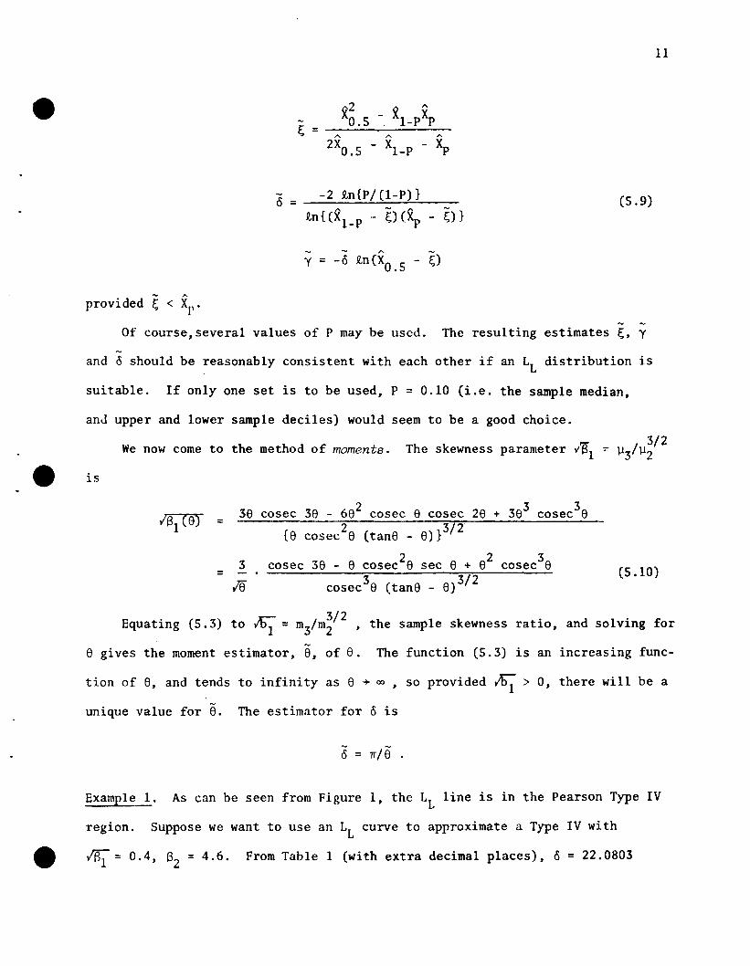
provided E;, < Xp •

-2 in{P/ (l-P)}o = --_....:-~-~---in{(X1_p - ~)(~

(5.9)

11

-Of course, several values of P may be used. The resulting estimates E;" y

-and 6 should be reasonably consistent with each other if an LL distribution is

suitable. If only one set is to be used, P = 0.10 (i.e. the sample median,

and upper cmd lower sample deciles) would seem to be a good choice.

e is

We now come to the method of moments. The skewness parameter i~l

38 38 - 682 cosec 8 cosec 3 318

1(8) cosec 28 + 38 cosec 8=

8)}3/2{8 2(tan8 -cosec 8

3 2 2 3cosec 38 - 8 cosec 8 sec 8 + 8 cosec 8 (5.10)= - .3 3/218 cosec 8 (tan8 - 8)

~ 3/2Equating (5.3) to vOl = m3/m2 • the sample skewness ratio, and solving for

8 gives the moment estimator, 8, of 8. The function (5.3) is an increasing func-

tion of 8, and tends to infinity as 8 ~ 00 , so provided ~ > 0, there will be a

unique value for 8. The estimator for 6 is

o = TI/e

Example 1. As can be seen from Figure 1, the LL line is in the Pearson Type IV

region. Suppose we want to use an LL curve to approximate a Type IV with

~ = 0.4. 82 = 4.6. From Table 1 (with extra decimal places), 0 = 22.0803

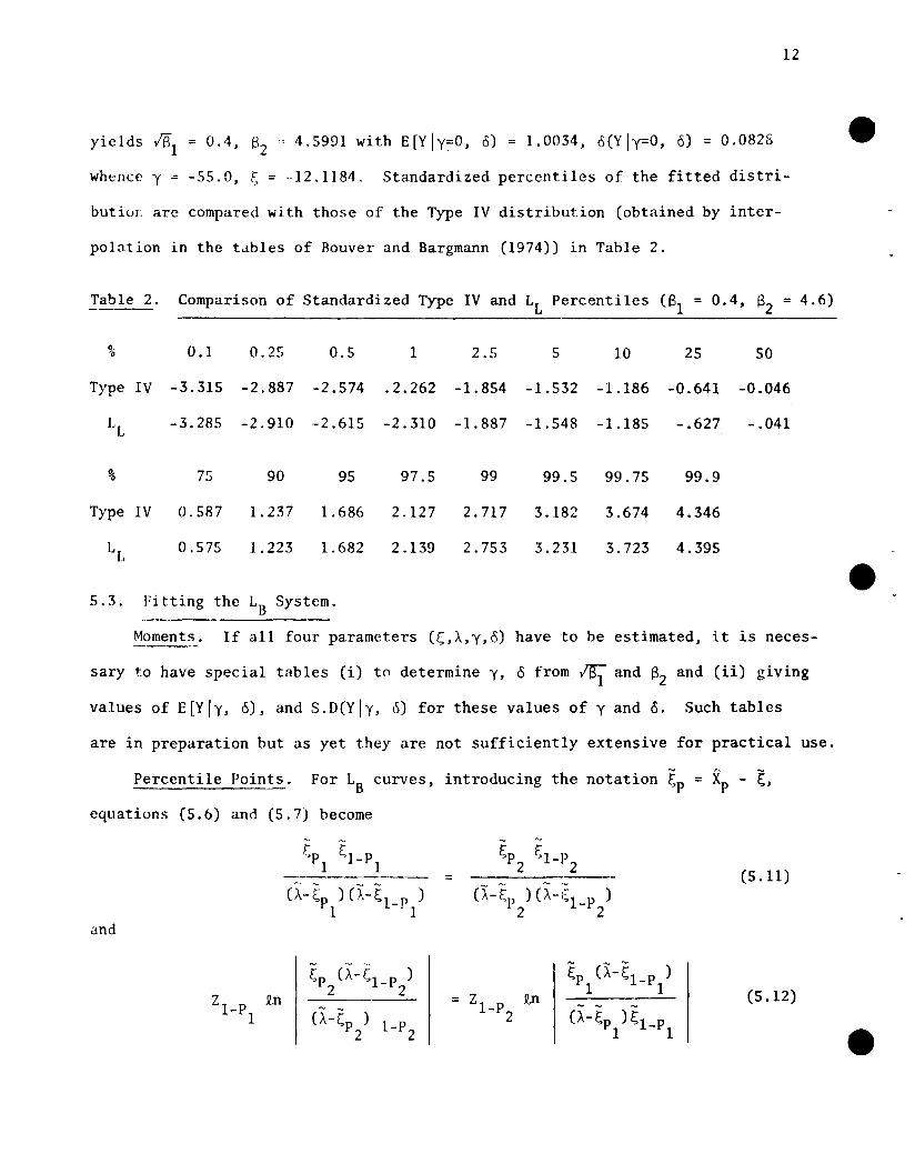
12

yields lSI = 0.4, 82 ,4.5991 with E[Yly=O, 8) = 1.0034, O(Yly=O, 8) = 0.0828

whence y = -55.0, (, = ·-12.1184. Standardized percentiles of the fitted distri-

butiol are compared with those of the Type IV distribution (obtained by inter-

polation in the tables of Bouver and Bargmann (1974)) in Table 2.

Table 2. Comparison of Standardized Type IV and LL Percentiles (81 = 0.4, 82 = 4.6)

90 0.1 0.25 0.5 1 2.5 5 10 25 50

Type IV -3.315 -2.887 -2.574 .2.262 -1. 854 -1.532 -1.186 -0.641 -0.046

LL -3.285 -2.910 -2.615 -2.310 -1. 887 -1.548 -1.185 -.627 -.041

% 75 90 95 97.5 99 99.5 99.75 99.9

Type IV 0.587 1. 237 1.686 2.127 2.717 3.182 3.674 4.346

LL 0.575 1.223 1.682 2.139 2.753 3.231 3.723 4.395

e5.3. Fitting the LB System.

Moments. If all four parameters (E;;,A,y,8) have to be estimated, it is neces------sary to have special tables (i) to determine y, 8 from 181 and 8

2and (ii) giving

values of E[Yly, 6), and s.D(Yly, 6) for these values of y and 6. Such tables

are in preparation but as yet they are not sufficiently extensive for practical use.

Percentile Points. For LB curves, introducing the notation ~P = Xp - t

equations (5.6) and (5.7) become

and

= (5.ll)

E:p (A-E:1_P )2 2

6-~p )Z I-P Z

~P CX-~l_P )1 1

- - -P'-~P ) ~l-P

1 1

(5.12)

13

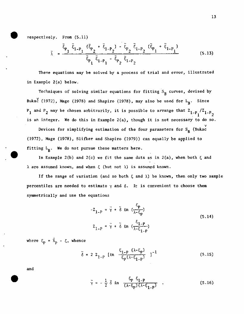
respectively. From (5.11)

-(~p +

-~P ~l-P ~l-P ) - ~ F;l_P (~p + ~l-P )

1 1 2 2 P2 2 1 1= - -

~l-P~P ~l-P - ~1 1 P2 2

These equations may be solved by a process of trial and error, illustrated

in Exan~le 2(a) below.

Techniques of solving similar equations for fitting S8 curves, devised by

vBukac (1972), Mage (1978) and Shapiro (1978), may also be used for LB' Since

PI and P2 may be chosen arbitrarily, it is possible to arrange that Zl_P /ZI_P.12

is an integer. We do this in Example 2(a), though it is not necessary to do so.v

Devices for simplifying estimation of the four parameters for SB (Bukac

(1972), Mage (1978), Slifker and Shapiro (1979)) can equally be applied to

fitting LB. We do not pursue these matters here.

In Example 2(b) and 2(c) we fit the same data as in 2(a), when both ~ and

A are assumed known, and when ~ (but not A) is assum~d known.

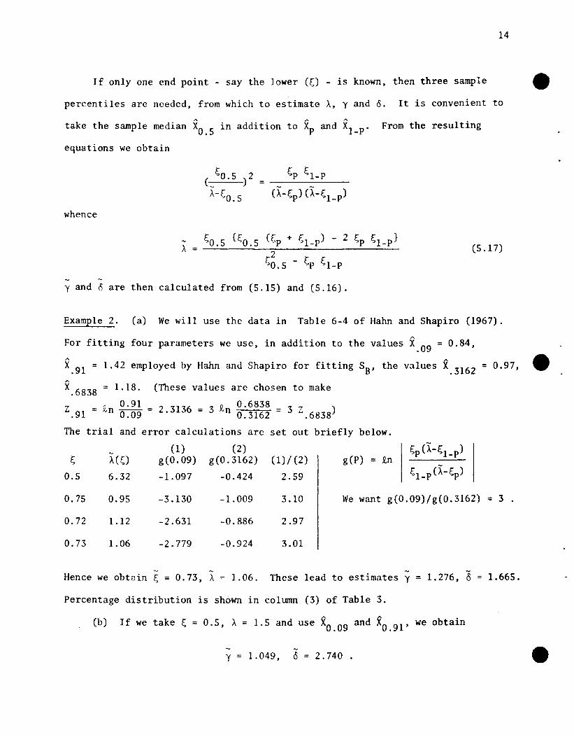
If the range of variation (and so both ; and A) be known, then only two sample

percentiles are needed to estimate y and o. It is convenient to choose them

symmetrically and use the equations

-Zl_P <5;P

= y + tIl (A-; )P

;Zl_P = Y + <5 £On ( l-P)

A-;I_P

"-

where ;P = Xp - ~, whence

(5.14)

-<5 = 2 Zl_P [£On

and

~l-P (A-~p)

~P ()..-f,;l_P)(5.15)

y - - 1. ;5 £On2

(5.16)

14

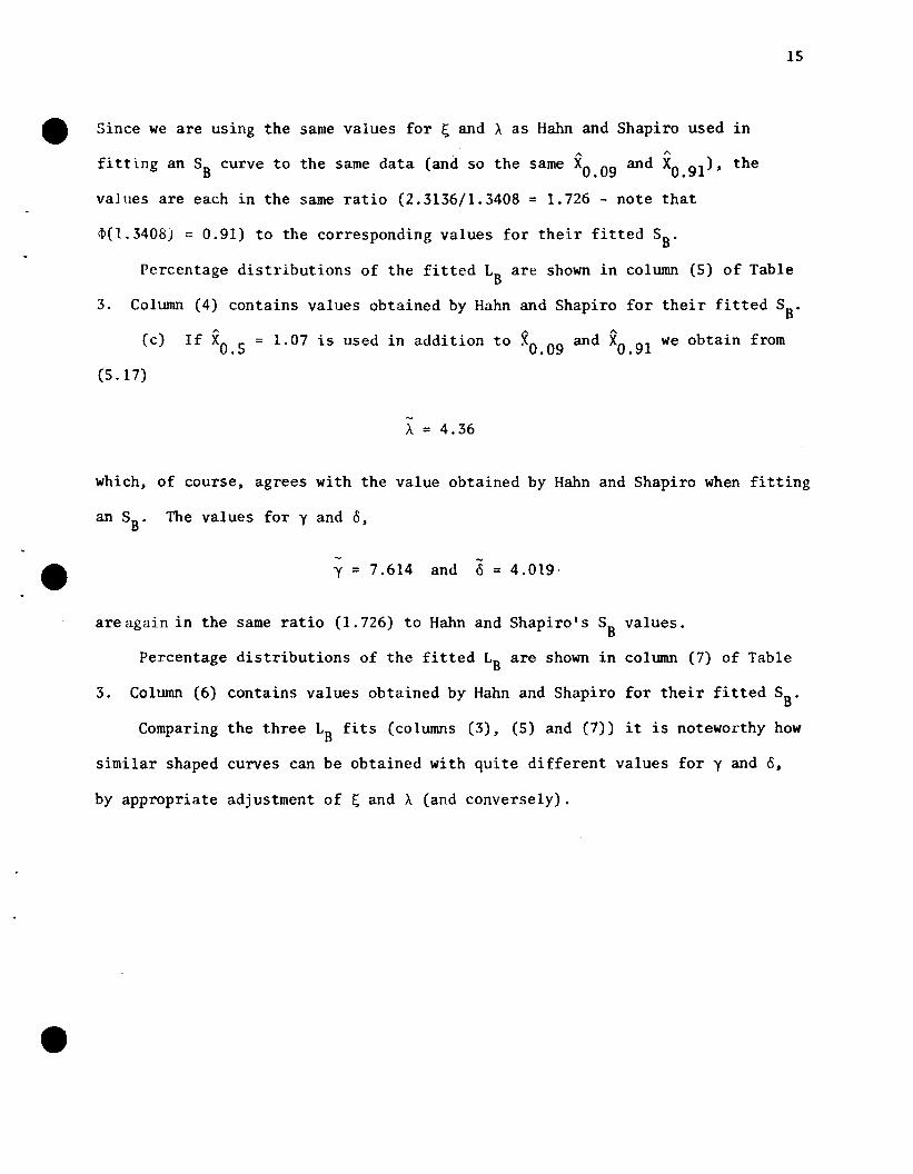
If only one end point - say the lower (E,) - is known, then three sample

percentiles are needed, from which to estimate A, y and o. It is convenient to

take the sample median XO. 5 in addition to Xp and Xl_po From the resulting

equations we obtain

whence

(5.17)

y and 0 are then calculated from (5.15) and (5.16).

Example 2. (a) We will use the data in Table 6-4 of Hahn and Shapiro (1967).

For fitting four parameters we use, in addition to the values X. 09 = 0.84,

X. 9l = 1.42 employed by Hahn and Shapiro for fitting S8' the values X. 3l62 = 0.97, ~A

X. 6838 = 1.18. (These values are chosen to make

Z n 0.91 - 2 3136 - 3 ~ 0.6838 - 3 ).91 = ~n 0.09 - . . - n 0.3162 - Z.6838

The trial and error calculations are set out briefly below.

- (1) (2) ~P (X-~l_P)~ A(E,) g(0.09) g(0.3l62) (1) / (2) g(P) = ,q,n

0.5 6.32 -1. 097 -0.424 2.59 ~l-P (X-~p)

0.75 0.95 -3.130 -1.009 3.10 We want g(0.09)/g(0.3l62) = 3 .

0.72 1.12 -2.631 -0.886 2.97

0.73 1.06 -2.779 -0.924 3.01

-Hence we obtain E, = 0.73, A ~ 1.06. These lead to estimates y = 1.276, 8

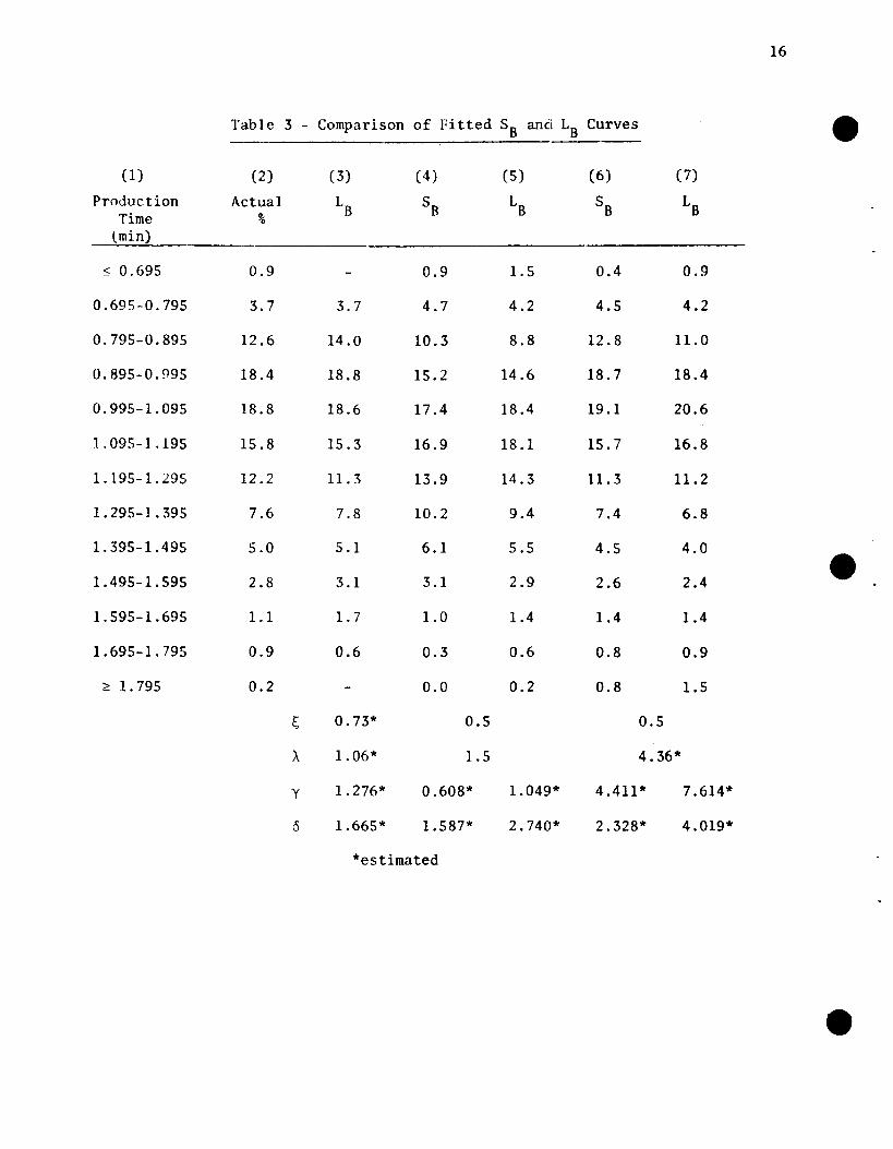
Percentage distribution is shown in column (3) of Table 3.

(b) If we take ~ = 0.5. A = 1.5 and use XO. 09 and XO.91 ' we obtain

-y = 1.049, 0 = 2.740 .

1.665.

15

~ Since we are using the same values for ~ and A as Hahn and Shapiro used in

fitting an SB curve to the same data (and so the same XO. 09 and XO. 91)' the

values are each in the same ratio (2.3136/1.3408 = 1.726 - note that

~(1.3408) = 0.91) to the corresponding values for their fitted 5B.

Percentage distributions of the fitted LB are shown in column (5) of Table

3. Column (4) contains values obtained by Hahn and Shapiro for their fitted S8'

(e) If XO. 5 = 1.07 is used in addition to XO. 09 and XO. 91 we obtain from

(5.17)

~

A = 4.36

which, of course, agrees with the value obtained by Hahn and Shapiro when fitting

an SB' The values for y and 0,

y = 7.614 and 0 = 4.019-

are again in the same ratio (1.726) to Hahn and Shapiro's SB values.

Percentage distributions of the fitted LB are shown in column (7) of Table

3. Column (6) contains values obtained by Hahn and Shapiro for their fitted SB'

Comparing the three LB fits (columns (3), (5) and (7)) it is noteworthy how

similar shaped curves can be obtained with quite different values for y and 6,

by appropriate adjustment of ~ and A (and conversely).

16

Table 3 - Comparison of Fitted 5B and LB Curves

(1) (2) (3) (4) (5) (6) (7)

Production Actual LB 5B

LB

5B

LBTime %

(min)

:c; 0.695 0.9 0.9 1.5 0.4 0.9

0.695-0.795 3.7 3.7 4.7 4.2 4.5 4.2

0.795-0.895 12.6 14.0 10.3 8.8 12.8 11.0

0.895-0.995 18.4 18.8 15.2 14.6 18.7 18.4

0.995-1. 095 18.8 18.6 17.4 18.4 19.1 20.6

1.095-1.195 15.8 15.3 16.9 18.1 15.7 16.8

1.195-1. 295 12.2 11.3 13.9 14.3 11. 3 11.2

1.295-1.395 7.6 7.8 10.2 9.4 7.4 6.8

1.395-1.495 5.0 5.1 6.1 5.5 4.5 4.0 e1.495-1.595 2.8 3.1 3.1 2.9 2.6 2.4

1. 595-1. 695 1.1 1.7 1.0 1.4 1.4 1.4

1. 695-1. 795 0.9 0.6 0.3 0.6 0.8 0.9

~ 1. 795 0.2 0.0 0.2 0.8 1.5

~ 0.73* 0.5 0.5

A 1.06* 1.5 4.36*

y 1.276* 0.608* 1.049* 4.411* 7.614*

0 1.665* 1.587* 2.740* 2.328* 4.019*

*estimated

17

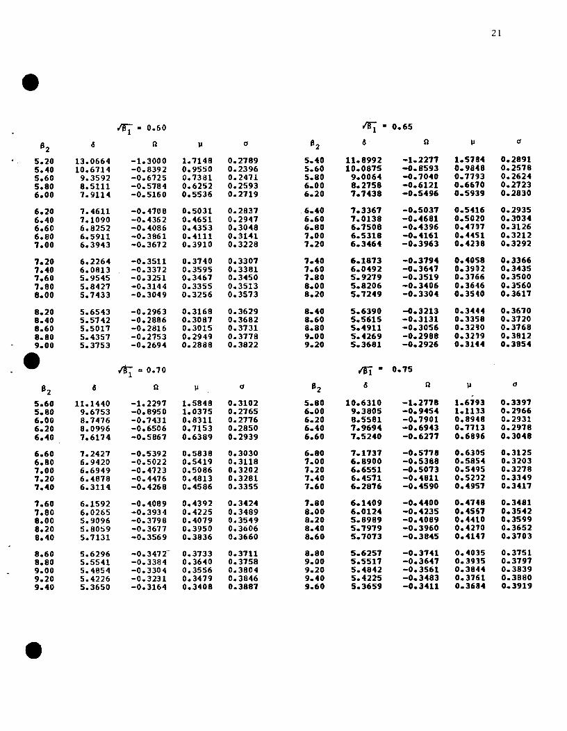
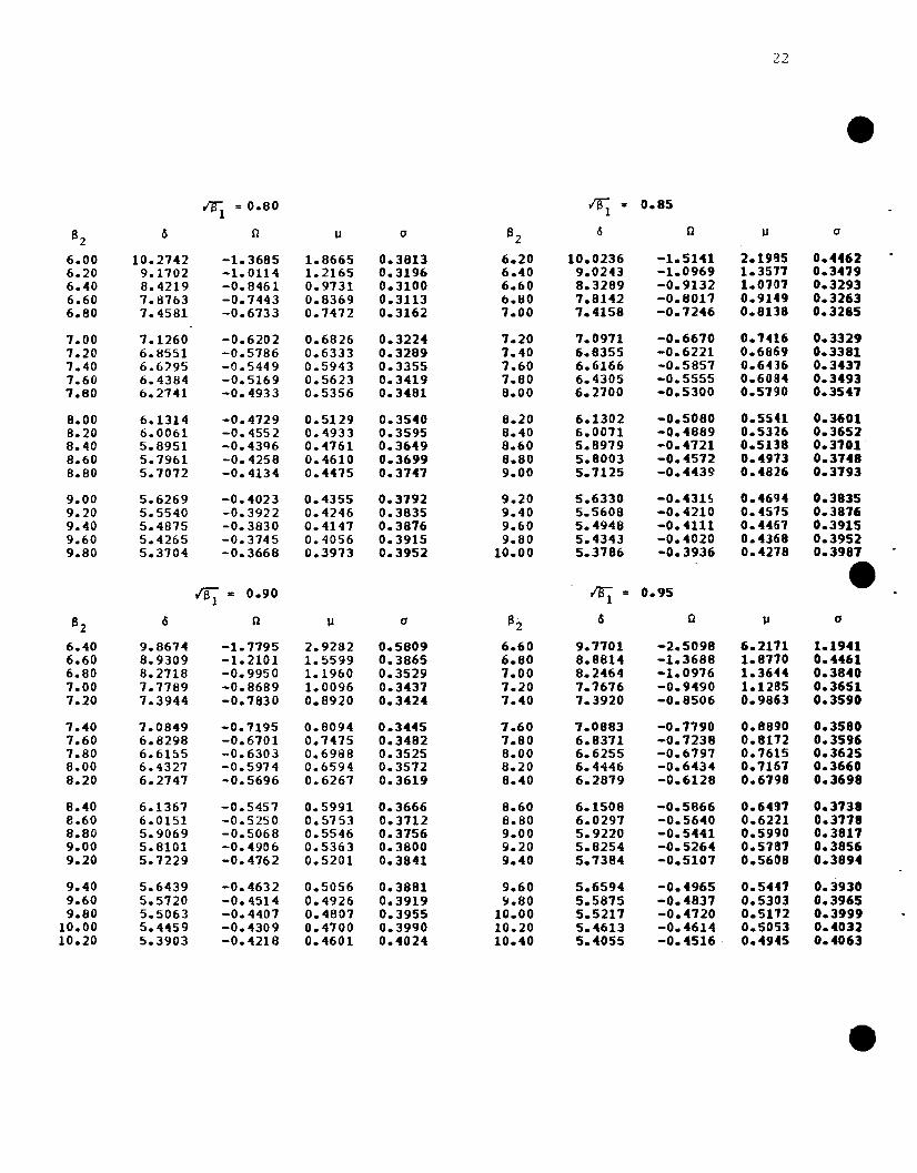
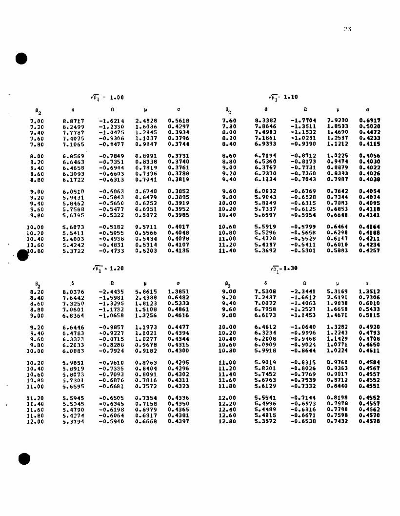
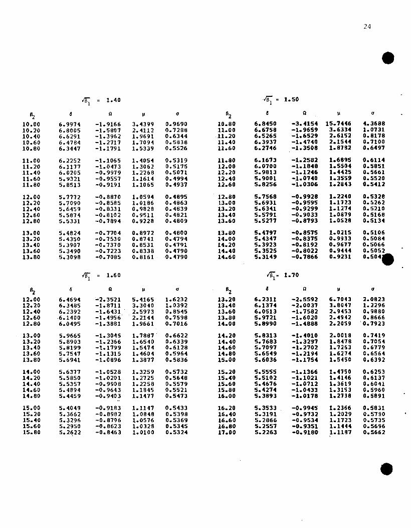
s.~. Fitting LU Distributions

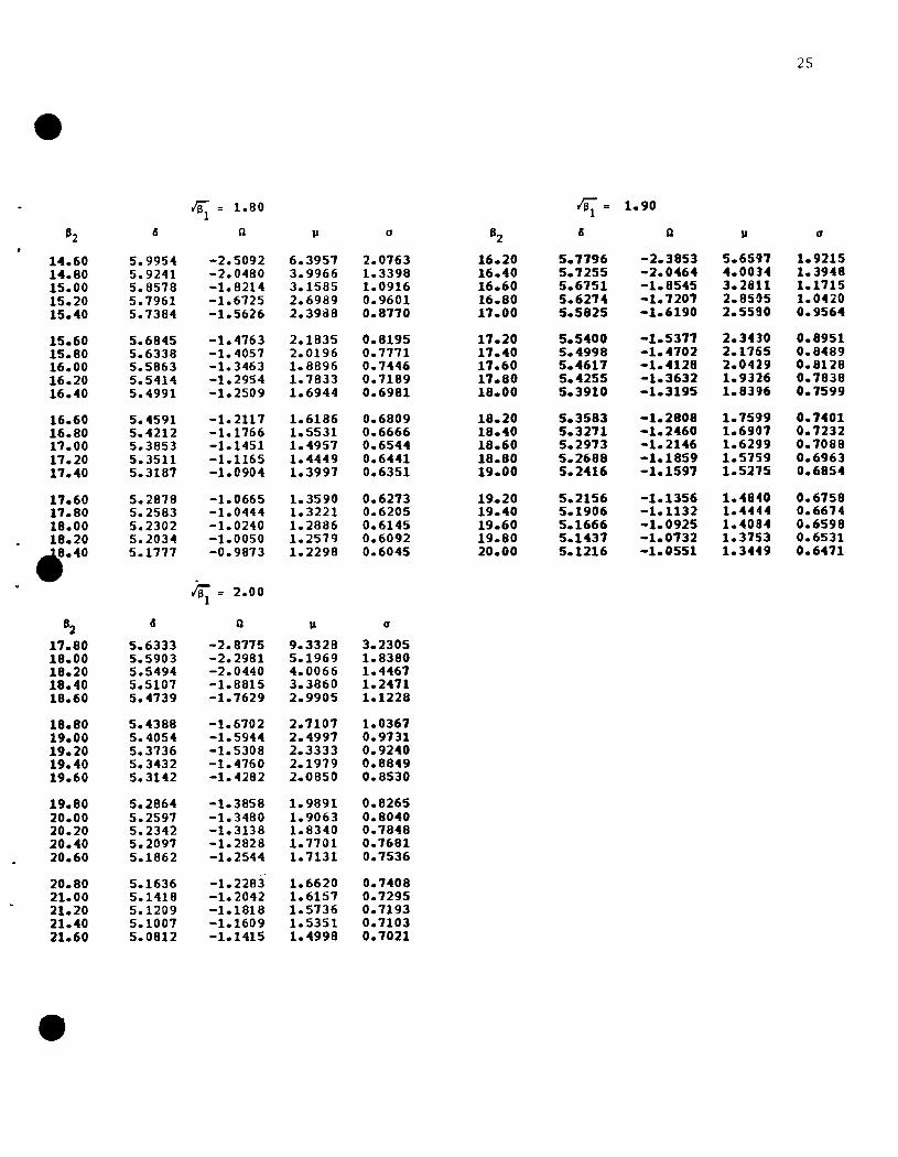
M0ments: Table 4 gives values of 0 and n(= Y/o). corresponding to

~ = 0.00CO.05)1(.1)2.0 combined (for each lSI) with twenty values of S2

increasing by intervals of 0.2. starting from a value just 'below' the LL line.

The simultaneous nonlinear equations

(5.18)

were solved for y and 0 using Brown's (1967) algorithm. The search for values of

n and 6 continued until I/Sl(y.o) - ~I ~ 10-6 and IS2(Y.o) - S2 1< 10-6 . The

use of the table is illustrated by the following example.

~ Example 3. We will compare a standardized Pearson Type IV curve with ~ = 0.9.

S2 = 8.6 against an LU curve having the same first four moments.

From Table 4 we obtain 0 = 6.0151 and n = -0.5250. where

y = 6.0151 x (-0.5250) = -3.1580. Using (4.7) we obtain

E[Y] = 0.5753; S.D. [V] = 0.3712 .

Using (5.4) (with 'observed' mean zero. and standard deviation 1) we obtain

-1A = (0.3712) = 2.6940. ~ = 0 - (2.6940 x 0.5753) = -1.5498. So the fitted

LU curve is defined by the statement that

Z = -3.1580 + 6.0151 sinh- l {(X + 1.5498/2.6940}

18

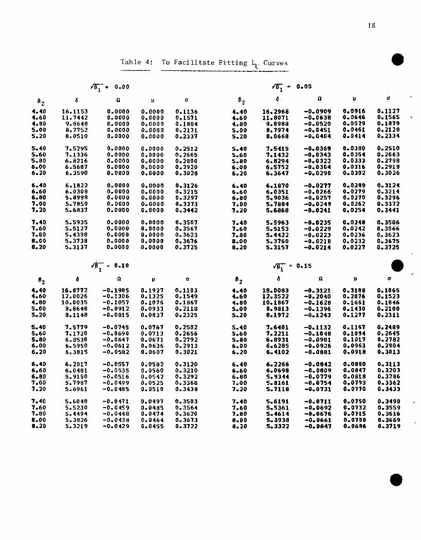
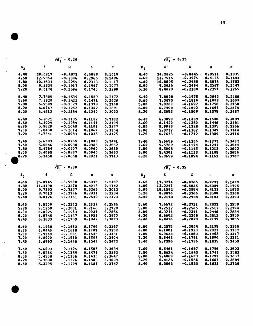
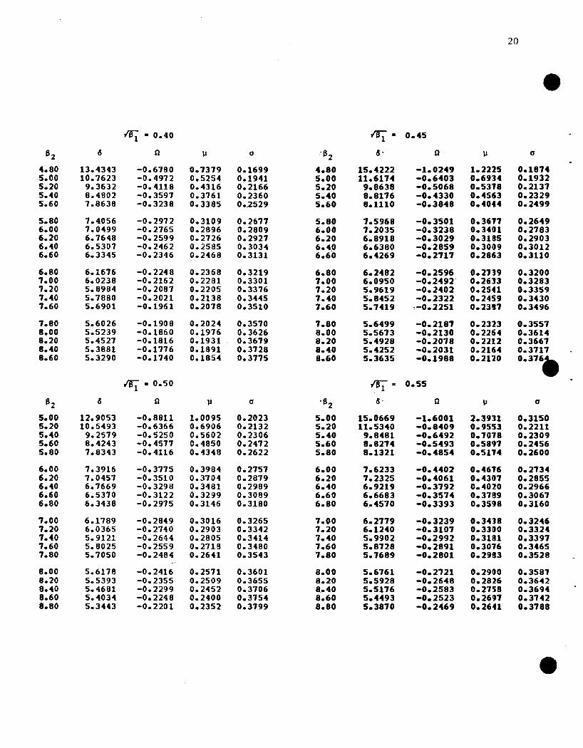
Table 4: To Facilitate Fitting LU

Curves

~. 0.00 r'B: • 0.051

11 2~ g \l a 11 2

~ g 1.1 a

4.40 16.1153 0.0000 0.0000 0.1136 4.40 16.2968 -0.0909 0.0916 0.11214.60 11.7442 0.0000 0.0000 0.1511 4.60 11.8011 -0.0638 0.0646 0.15654.80 9.8648 0.0000 0.0000 0.1884 4.80 9.8988 -0.0520 0.0529 0.18195.00 8.7752 0.0000 0.0000 0.2131 5.00 8.1914 -0.0451 0.0461 0.21285.20 8.0510 0.0000 0.0000 0.2331 5.20 8.0668 -0.0404 0.0414 0.2334

5.40 1.5295 0.0000 0.0000 0.2512 5.40 1.5415 -0.0369 0.0380 0.25105.60 1.1336 0.0000 0.0000 0.2665 5.60 1.1432 -0.0343 0.0354 0.26635.80 6.8216 0.0000 0.0000 0.2800 5.80 6.8294 -0.0322 0.0313 0.21986.00 6.5681 0.0000 0.0000 0.2920 6.00 6.5152 -0.0304 0.0316 0.29186.20 6.3590 0.0000 0.0000 0.3028 6.20 6.3641 -0.0290 0.0302 0.3026

6.40 6.1822 0.0000 0.0000 0.3126 6.40 6.1810 -0.0211 0.0289 0.31246.60 6.0308 0.0000 0.0000 0.3215 6.60 6.0351 -0.0266 0.0219 0.32146.80 5.8998 0.0000 0.0000 0.3291 6.80 5.9036 -0.0251 0.0210 0.32961.00 5.7850 0.0000 0.0000 0.3313 1.00 5.1884 -0.0249 0.0252 0.33721.20 5.6831 0.0000 0.0000 0.3442 7.20 5.6868 -0.0241 0.0254 0.3441

1.40 5.5935 0.0000 0.0000 0.3501 7.40 5.5963 -0.0235 0.0248 0.35061.60 5.5121 0.0000 0.0000 0.3567 1.60 5.5153 -0.0229 0.0242 0.35661.80 5.4398 0.0000 0.0000 0.3623 7.80 5.4422 -0.0223 0.0236 0.36238.00 5.3738 0.0000 0.0000 0.3616 8.00 5.3760 -0.0218 0.0232 0.36158.20 5.3131 0.0000 0.0000 0.3125 8.20 5.3157 -0.0214 0.0227 0.3725

~ = 0.10 IB. = 0.15 e1 1

82 cS n 1J a 11 2 cS n lJ a

4.40 16.8772 -0.1905 0.1921 0.1103 4.40 1&.0083 -0.3121 0.3188 0.10654.60 12.0026 -0.1306 0.1325 0.1549 4.60 12.3522 -0.2040 0.2016 0.15234.80 10.0035 -0.1051 0.1016 0.1861 4.80 10.1861 -0.1628 0.1651 0.18465.00 8.8648 -0.0912 0.0933 0.2118 5.00 8.9813 -0.1396 0.1430 0.21005.20 8.1148 -0.0815 0.0831 0.2325 5.20 8.1912 -0.1243 0.1211 0.2311

5.40 7.5119 -0.0145 0.0767 0.2502 5.40 1.6401 -0.1132 0.1151 0.24895.60 7.1120 -0.0690 0.0113 0.2656 5.60 1.2211 -0.104& 0.1084 0.26455.80 6.8530 -0.0641 0.0611 0.2192 5.80 6.8931 -0.091J1 0.1011 0.27826.00 6.5950 -0.0612 0.0636 0.2913 6.00 6.6285 -0.0926 0.0963 0.29046.20 6.3815 -0.0582 0.0607 0.3021 6.20 6.4102 -0.0881 0.0918 0.3013

6.40 6.2011 -0.0551 0.0582 0.3120 6.40 6.2266 -0.0842 0.0880 0.31136.60 6.0481 -0.0535 0.0560 0.3210 6.60 6.0698 -0.0809 0.0841 0.32036.80 5.9150 -0.0516 0.0542 0.3292 6.80 5.9344 -0.0779 0.0818 0.32861.00 5.1987 -0.0499 0.0525 0.3368 7.00 5.8161 -0.0154 0.0193 0.33627.20 5.6961 -0.0485 0.0510 0.3438 1.20 5.1118 -0.0131 0.0110 0.3433

1.40 5.6048 -0.0471 0.0497 0.3503 1.40 5.6191 -0.0111 0.0150 0.34987.60 5.5230 -0.0459 0.0485 0.3564 1.60 5.5361 -0.0692 0.0132 0.35597.80 5.4494 -0.0448 0.0414 0.3620 1.80 5.4614 -0.0616 0.0115 0.36168.00 5.3826 -0.0438 0.0464 0.3673 8.00 5.3938 -0.0661 o.ono 0.36698.20 5.3219 -0.0429 0.0455 0.3122 8.20 5.3322 -0.0641 0.0686 0.3119

19

~= 0.20 fli""" = 0.25

B2 15 0 lJ a B215- 0 lJ a

4.40 20.0811 -0.4873 0.5089 0.1019 4.40 24.2825 -0.8445 0.9511 0.10354.60 12.9064 -0.2896 0.2966 0.1486 4.60 13.7515 -0.3915 0.4116 0.14444.80 10.4634 -0.2259 0.2313 0.1817 4.80 10.8595 -0.2985 0.3013 0.11825.00 9.1539 -0.1917 0.1967 0.2077 5.00 9.3936 -0.2494 0.2561 0.20415.20 8.3178 -0.1696 0.1745 0.2290 5.20 8.4828 -0.2188 0.2251 0.2265

5.40 7.7305 -0.1539 0.1589 0.2412 5.40 1.8528 -0.1915 0.2042 0.24505.60 7.2920 -0.1421 0.1471 0.2629 5.60 1.3815 -0.1816 0.1831 0.26095.80 6.9509 -0.1327 0.1378 0.2768 5.80 1.0280 -0.1692 0.1158 0.27506.00 6.6767 -0.1252 0.1302 0.2891 6.00 6.1408 -0.1592 0.1658 0.28156.20 6.4512 -0.1189 0.1240 0.3002 6.20 6.5055 -0.1509 0.1515 0.2981

6.40 6.2621 -0.1135 0.1181 0.3102 6.40 6.3090 -0.1439 0.1506 0.30896.60 6.1009 -0.1089 0.1141 0.3194 6.60 6.1420 -0.1380' 0.1446 0.31816.80 5.9620 -0.1049 0.1101 0.3277 6.80 5.9983 -0.1328 0.1395 0.32661.00 5.8408 -0.1014 0.1067 0.3354 1.00 5.8132 -0.1282 0.1349 0.33441.20 5.7341 -0.0983 0.1036 0.3425 7.20 5.1633 -0.1242 0.1309 0.3416

7.40 5.6393 -0.0955 0.1008 0.3491 1.40 5.6659 -0.1206 0.1213 0.34821.60 5.5546 -0.0930 0.0983 0.3552 1.60 5.5189 -0.1114 0.1241 0.35441.80 5.4784 -0.0901 0.0960 0.3610 7.80 5.5008 -0.1145 0.1212 0.36028.00 5.4095 -0.0887 0.0940 0.3663 8.00 5.4301 -0.1118 0.1185 0.3656

,,8.20 5.3468 -0.0868 0.0921 0.3113 8.20 5.3659 -0.1094 0.1161 0.3101

iBt • 0.30 1Bl- 0.35

S 4 0 lJ a B2 4 0 lJ a2

4.60 15.0145 -0.5508 0.5833 0.1401 4.60 11.3274 -0.8266 0.9291 0.14394.80 11.4198 -0.3870 0.4018 0.1742 4.80 12.2241 -0.5035 0.5309 0.11055.00 9.7192 -0.3157 0.3266 0.2012 5.00 10.1592 -0.3954 0.4123 0.19755.20 8.1013 -0.2736 0.2831 0.2234 5.20 8.9816 -0.3366 0.3500 0.22005.40 8.0126 -0.2451 0.2540 0.2423 5.40 8.2118 -0.2984 0.3103 0.2393

5.60 7.5109 -0.2242 0.2329 0.2586 5.60 1.6612 -0.2711 0.2823 0.25595.80 7.1269 -0.2081 0.2166 0.2729 5.80 1.2512 -0.2505 0.2612 0.27046.00 6.8225 -0.1953 0.2031 0.2856 6.00 6.9244 -0.2341 0.2446 0.28346.20 6.5145 -0.1847 0.1931 0.2970 6.20 6.6602 -0.2208 0.2311 0.29506.40 6.3683 -0.1759 0.1842 0.3013 6.40 6.4416 -0.2098 0.21<J9 0.3055

6.60 6.1938 -0.1683 0.1766 0.3167 6.60 6.2515 -0.2004 0.2105 0.31506.80 6.0440 -0.1618 0.1101 0.3252 6.80 6.1001 -0.1923 0.2023 0.32371.00 5.9140 -0.1561 0.1643 0.3331 1.00 5.9638 -0.1853 0.1953 0.33171.20 5.8000 -0.1510 0.1593 0.3404 7.20 5.8448 -0.1791 0.18CJO 0.33911.40 5.6992 -0.1466 0.1548 0.3412 1.40 5.1396 -0.1136 0.1835 0.3459

7.60 5.6093 -0.1425 0.1508 0.3534 7.60 5.6461 -0.1681 0.1186 0.35231.80 5.5286 -0.1389 0.1471 0.3593 7.80 5.5624 -0.1643 0.1141 0.35828.00 5.4558 -0.1356 0.1438 0.3641 8.00 5.4869 -0.1603 0.1101 0.36378.20 5.3898 -0.1326 0.1408 0.3699 8.20 5.4186 -0.1566 0.1664 0.36898.40 5.3295 -0.1299 0.1381 0.3141 8.40 5.3563 -0.1533 0.1631 0.3138

20

IBl - 0.40 I!"i"- 0.45

62 6 0 1.1 0 -62

6- 0 1.1 a

4.80 13.4343 -0.6180 0.1319 0.1699 4.80 15.4222 -1.0249 1.2215 0.18145.00 10.7623 -0.4972 0.5254 0.1941 5.00 11.6114 -0.6403 0.6934 0.19325.20 9.3632 -0.4118 0.4316 0.2166 5.20 9.8638 -0.5068 0.5318 0.21315.40 8.4802 -0.3591 0.3161 0.2360 5.40 8.8116 -0.4330 0.4563 0.23295.60 1.8638 -0.3238 0.3385 0.,2529 5.60 8.1110 -0.3848 0.4044 0.2499

5.80 1.4056 -0.2972 0.3109 0.2617 5.80 1.5968 -0.3501 0.3611 0.26496.00 1.0499 -0.2765 0.2896 0.2809 6.00 1.2035 -0.3238 0.3401 0.27836.20 6.7648 -0.2599 0.2726 0.2927 6.20 6.8918 -0.3029 0.3185 0.29036.40 6.5307 -0.2462 0.2585 0.3034 6.40 6.6380 -0.2859 0.3009 0.30126.60 6.3345 -0.2346 0.2468 0.3131 6.60 6.4269 -0.2111 0.2863 0.3110

6.80 6.1676 -0.2248 0.2368 0.3219 6.80 6.2482 -0.2596 0.2139 0.32001.00 6.0238 -0.2162 0.2281 0.3301 1.00 6.0950 -0.2492' 0.2633 0.32837.20 5.8984 -0.2087 0.2205 0.3376 7.20 5.9619 -0.2402 0.2541 0.33597.40 5.1880 -0.2021 0.2138 0.3445 1.40 5.8452 -0.2322 0.2459 0.34307.60 5.6901 -0.1961 0.2018 0.3510 1.60 5.7419 --0.2251 0.2311 0.3496

7.80 5.6026 -0.1908 0.2024 0.3570 7.80 5.6499 -0.2181 0.2313 0.35578.00 5.5239 -0.1860 0.1916 0.3626 8.00 5.5613 -0.2130 0.2264 0.36148.20 5.4527 -0.1816 0.1931 0.3679 8.20 5.4928 -0.2018 0.2212 0.36618.40 5.3881 -0.1"116 0.1891 0.3728 8.40 5.4252 -0.2031 0.2164 0.31118.60 5.3290 -0.1740 0.1854 0.3715 8.60 5.3635 -0.1988 0.2120 0.316.

IBl - 0.50 I!l- 0.55

62 6 0 1.1 a -6 2 6' 0 1.1 a

5.00 12.9053 -0.8811 1.0095 0.2023 5.00 15.0669 -1.6001 2.3931 0.31505.20 10.5493 -0.6366 0.6906 0.2132 5.20 11.5340 -0.8409 0.9553 0.22115.40 9.2519 -0.5250 0.5602 0.2306 5.40 9.8481 -0.6492 0.1018 0.23095.60 8.4243 -0.4517 0.4850 0.2472 5.60 8.8214 -0.5493 0.5891 0.24565.80 7.8343 -0.4116 0.4348 0.2622 5.80 8.1321 -0.4854 0.5114 0.2600

6.00 7.3916 -0.3775 0.3984 0.2757 6.00 1.6233 -0.4402 0.4616 0.27346.20 7.0451 -0.3510 0.3704 0.2879 6.20 7.2325 -0.4061 0.4301 0.28556.40 6.1669 -0.3298 0.3481 0.2989 6.40 6.9219 -0.3192 0.4020 0.29666.60 6.5370 -0.3122 0.3B9 0.3089 6.60 6.6683 -0.3514 0.3189 0.30616.80 6.3438 -0.2975 0.3146 0.3180 6.80 6.4510 -0.3393 0.3598 0.3160

1.00 6.1189 -0.2849 0.3016 0.3265 7.00 6.2179 -0.3239 0.3438 0.32461.20 6.0365 -0.2140 0.2903 0.3342 7.20 6.1240 -0.3101 0.3300 0.33247.40 5.9121 -0.2644 0.2805 0.3414 1.40 5.9902 -0.2992 0.3181 0.33917.60 5.8025 -0.2559 0.2119 0.3480 1.60 5.8728 -0.2891 0.3016 0.34651.80 5.1050 -0.2484 0.2641 0.3543 1.80 5.1689 -0.2801 0.2983 0.3528

8.00 5.6178 -0.2416 0.2511 0.3601 8.00 5.6161 -0.2121 0.29aO 0.35818.20 5.5393 -0.2355 0.2509 0.3655 8.20 5.5928 -0.2648 0.2826 0.36428.40 5.4681 -0.2299 0.2452 0.3706 8.40 5.5116 -0.2583 0.2158 0.36948.60 5.4034 -0.2248 0.2400 0.3154 8.60 5.4493 -0.2523 0.2691 0.31428.80 5.3443 -0.2201 0.2352 0.3199 8.80 5.3810 -0.2469 0.2641 0.3188

21

IBl • 0.60 t'1"i • 0.65

826 0 lJ a 82 6 0 lJ a

5.20 13.0664 -1.3000 1.1148 0.2789 5.40 11.8992 -1.2271 1.5184 0.28915.40 10.6714 -0.8392 0.9550 0.2396 5.60 10.0815 -0.8593 0.9848 0.25185.60 9.3592 -0.6725 0.7381 0.2471 5.80 9.0064 -0.1040 0.7193 0.26245.80 8.5111 -0.5184 0.6252 0.2593 6.00 8.2158 -0.6121 0.6610 0.27236.00 7.9114 -0.5160 0.5536 0.2119 6.20 1.7438 -0.5496 0.5939 0.2830

6.20 1.4611 -0.4108 0.5031 0.2831 6.40 1.3361 -0.5031 0.5416 0.29356.40 1.1090 -0.4362 0.4651 0.2947 6.60 1.0138 -0.4681 0.5020 0.30346.60 6.8252 -0.4086 0.4353 0.3048 6.80 6.1508 -0.4396 0.47n 0.31266.80 6.5911 -0.3861 0.4111 0.3141 7.00 6.5318 -0.4161 0.4451 0.32121.00 6.3943 -0.3672 0.3910 0.3228 1.20 6.3464 -0.3963 0.4218 0.3292

1.20 6.2264 -0.3511 0.3740 0.3301 1.40 6.1813 -0.3194 0.4058 0.33661.40 6.0813 -0.3312 0.3595 0.3381 1.60 6.0492 -0.3641 0.391)2 0.34351.60 5.9545 -0.3251 0.3467 0.3450 1.80 5.9219 -0.3519 0.3766 0.35007.80 5.8421 -0.3144 0.3355 0.3513 8.00 5.8206 -0.3406 0.3646 0.35608.00 5.1433 -0.3049 0.3256 0.3513 8.20 5.1249 -0.3304 0.3540 0.3617

8.20 5.6543 -0.2963 0.3168 0.3629 8.40 5.6390 -0.3213 0.3444 0.36108.40 5.5142 -0.2886 0.3081 0.3682 8.60 5.5615 -0.3131 0.3358 0.31208.60 5.5017 -0.2816 0.3015 0.3731 8.80 5.4911 -0.3056 0.3230 0.31688.80 5.4351 -0.2153 0.2949 0.3718 9.00 5.4269 -0.2988 0.321)9 0.38129.00 5.3153 -0.2694 0.288a 0.3822 9.20 5.3681 -0.2926 0.3144 0.3854

e Iti' • 0.10 Ifi • 0.15

82 6 0 lJ a 82 6 0 lJ a

5.60 11.1440 -1.2297 1.5848 0.3102 5.80 10.6310 -1.2118 1.611J3 0.33915.80 9.6153 -0.8950 1.0375 0.2765 6.00 9.3805 -0.9454 1.1113 0.29666.00 8.7416 -0.1431 0.8311 0.2116 6.20 8.5581 -0.7901 0.8948 0.29316.20 8.0996 -0.6506 0.1153 0.2850 6.40 1.9694 -0.6943 0.1713 0.29186.40 7.6174 -0.5861 0.6389 0.2939 6.60 1.5240 -0.6217 0.6896 0.3048

6.60 1.2421 -0.5392 0.5838 0.3030 6.80 1.1131 -0.5118 0.6305 0.31256.80 6.9420 -0.5022 0.5419 0.3118 1.00 6.8900 -0.5388 0.5854 0.32031.00 6.6949 -0.4123 0.5086 0.3202 1.20 6.6551 -0.5013 0.5495 0.32187.20 6.4878 -0.4416 0.4813 0.3281 1.40 6.4511 -0.4811 0.52n 0.33491.40 6.3114 -0.4268 0.4586 0.3355 1.60 6.2816 -0.4590 0.4951 0.3411

7.60 6.1592 -0.4089 0.4392 0.3424 7.80 6.1409 -0.4400 0.4748 0.34811.80 6.0265 -0.3934 0.4225 0.3489 8.00 6.0124 -0.4235 0.4551 0.35428.00 5.9096 -0.3198 0.4079 0.3549 8.20 5.8989 -0.4089 0.4410 0.35998.20 5.8059 -0.3617 0.3950 0.3606 8.40 5.1919 -0.3960 0.4210 0.36528.40 5.1131 -0.3569 0.3836 0.3660 8.60 5.1013 -0.3845 0.4141 0.3103

8.60 5.6296 -0.3412'· 0.3733 0.3711 8.80 5.6251 -0.3141 0.4035 0.31518.80 5.5541 -0.3384 0.3640 0.3758 9.00 5.5511 -0.3647 0.3915 0.31919.00 5.4854 -0.3304 0.3556 0.3804 9.20 5.4842 -0.3561 0.3844 0.38399.20 5.4226 -0.3231 0.3419 0.3846 9.40 5.4225 -0.3483 0.3761 0.38809.40 5.3650 -0.3164 0.3408 0.3881 9.60 5.3659 -0.3411 0.3684 0.3919

22

Ilri =0.80 lSi 0.85

626 11 II C1 62

6 11 II a

6.00 10.2742 -1.3685 1.8665 0.3813 6.20 10.0236 -1.5141 2.19115 0.44626.20 9.1702 -1.0114 1.2165 0.3196 6.40 9.0243 -1.0969 1.3517 0.34196.40 8.4219 -0.8461 0.9131 0.3100 6.60 8.3289 -0.9132 1.0101 0.32936.60 1.8163 -0.1443 0.8369 0.3113 6.80 7.8142 -0.8017 0.9149 0.32636.80 1.4581 -0.6733 0.1412 0.3162 1.00 7.4158 -0.7246 0.8138 0.3285

7.00 7.1260 -0.6202 0.6826 0.3224 7.20 7.0971 -0.6670 0.7416 0.33291.20 6.8551 -0.5786 0.6333 0.3289 7.40 6.8355 -0.6221 0.6869 0.33811.40 6.6295 -0.5449 0.5943 0.3355 7.60 6.6166 -0.5857 0.6436 0.34311.60 6.4384 -0.5169 0.5623 0.3419 7.80 6.4305 -0.5555 0.6084 0.34937.80 6.2141 -0.4933 0.5356 0.3481 8.00 6.2100 -0.5300 0.5190 0.3541

8.00 6.1314 -0.4729 0.5129 0.3540 8.20 6.1302 -0.5080 0.5541 0.36018.20 6.0061 -0.4552 0.4933 0.3595 8.40 6.0011 -0.4889 0.5326 0.36528.40 5.8951 -0.43Q6 0.4761 0.3649 8.60 5.8979 -0.4721 0.5H8 0.31018.60 5.1961 -0.4258 0.4610 0.3699 8.80 5.8003 -0.4572 0.4913 0.31488.80 5.1072 -0.4134 0.4415 0.3747 9.00 5.1125 -0.4439 0.4826 0.3193

9.00 5.6269 -0.4023 0.4355 0.3192 9.20 5.6330 -0.43B 0.4694 0.38359.20 5.5540 -0.3922 0.4246 0.3835 9.40 5.5608 -0.4210 0.4515 0.38169.40 5.4815 -0.3830 0.4141 0.3876 9.60 5.4948 -0.4111 0.4467 0.39159.60 5.4265 -0.3145 0.4056 0.3915 9.80 5.4343 -0.4020 0.4368 0.39529.80 5.3104 -0.3668 0.3913 0.3952 10.00 5.3186 -0.3936 0.4218 0.3987

ff. = 0.90 ~ 0.95e

=1

62 6 11 II C1 6 6 11 II C12

6.40 9.8674 -1.7195 2.9282 0.5809 6.60 9.7701 -2.5098 6.2111 1.19416.60 8.9309 -1.2101 1.5599 0.3865 6.80 8.8814 -1.3688 1.8110 0.44616.80 8.2118 -0.9950 1.1960 0.3529 7.00 8.2464 -1.0976 1.3644 0.38407.00 1.1189 -0.8689 1.0096 0.3437 7.20 7.7676 -0.9490 1.1285 0.36517.20 7.3944 -0.7830 0.8920 0.3424 7.40 7.3920 -0.8506 0.9863 0.3590

7.40 7.0849 -0.7195 0.8094 0.3445 7.60 1.0883 -0.7790 0.8890 0.35807.60 6.8298 -0.6701 0.1415 0.3482 7.80 6.8311 -0.7238 0.8112 0.35961.80 6.6155 -0.6303 0.6988 0.3525 8.00 6.6255 -0.6797 0.7615 0.36258.00 6.4327 -0.5914 0.6594 0.3572 8.20 6.4446 -0.6434 0.7161 0.36608.20 6.2141 -0.5696 0.6261 0.3619 8.40 6.2819 -0.6128 0.6198 0.3698

8.40 6.1361 -0.5451 0.5991 0.3666 8.60 6.1508 -0.5866 0.6431 0.31388.60 6.0151 -0.5250 0.5753 0.3712 8.80 6.0297 -0.5640 0.6221 0.31788.80 5.9069 -0.5068 0.5546 0.3156 9.00 5.9220 -0.5441 0.5990 0.38119.00 5.8101 -0.4906 0.5363 0.3800 9.20 5.8254 -0.5264 0.5181 0.38569.20 5.7229 -0.4762 0.5201 0.3841 9.40 5.7384 -0.5107 0.5608 0.3894

9.40 5.6439 -0.4632 0.5056 0.3881 9.60 5.6594 -0.4965 0.5441 0.39309.60 5.5120 -0.4514 0.4926 0.3919 9.80 5.5875 -0.4837 0.5303 0.39659.80 5.5063 -0.4401 0.4807 0.3955 10.00 5.5211 -0.4720 0.5112 0.3999

10.00 5.4459 -0.4309 0.4100 0.3990 10.20 5.4613 -0.4614 0.5053 0.403210.20 5.3903 -0.4218 0.4601 0.4024 10.40 5.4055 -0.4516 0.4945 0.4063

lSi =1.00 rs;= 1.10

/32c5 n 1I a B2 " n II a

7.00 8.8717 -1.6214 2.4828 0.5618 7.60 8.3382 -1.7704 2.9200 0.691'17.20 8.2499 -1.2330 1.6086 0.4297 7.80 7.8646 -1.3511 1.8503 0.50207.40 7.7787 -1.0475 1.2845 0.3934 a.oo 7.4903 -1.1532 1.4690 0.44127.60 7.4075 -0.9306 1.1037 0.3796 8.20 1.1861 -1.0281 1.2587 0.42337.80 7.1065 -0.8477 0.9847 0.3744 8.40 6.9333 -0.9390 1.1212 0.4115

8.00 6.8569 -0.7849 0.8991 0.3731 8.60 6.7194 -0.8712 1.0225 0.40568.20 6.6463 -0.7351 0.8338 0.3740 8.80 6.5360 -0.8173 0.9414 0.40308.40 6.4658 -0.6944 0.7819 0.3761 9.00 6.3767 -0.7731 0.8819 0.40228.60 6.3093 -0.6603 0.7396 0.3788 9.20 6.2370 -0.7360 0.8393 0.40268.80 6.1722 -0.6313 0.7041 0.3819 9.40 6.1134 -0.7043 O.n87 0.4038

9.00 6.0510 -0.6063 0.6740 0.3852 9.60 6.0032 -0.6769 0.1642 0.40549.20 5.9431 -0.5843 0.6479 0.3885 9.80 5.9043 -0.6528 0.7344 0.40749.40 5.8462 -0.5650 0.6252 0.3919 10.00 5.8149 -0.6315 0.7083 0.40959.60 5.7588 -0.5477 0.6051 0.3952 10.20 5.1337 -0.6125 0.6853 0.41189.80 5.6795 -0.5322 0.5872 0.3985 10.40 5.6597 -0.5954 0.6648 0.4141

10.00 5.6073 -0.5182 0.5711 0.4011 10.60 5.5919 -0.5799 0.6464 0.416410.20 5.5411 -0.5055 0.5566 0.4048 10.80 5.5296 -0.5658 0.6298 0.418810.40 5.4803 -0.4938 0.5434 0.4078 11.00 5.4720 -0.5529 0.6147 0.421110.60 5.4242 -0.4831 0.5314 0.4101 11.20 5.4187 -0.5411 0.6010 0.4234

. _0.80 5.3722 -0.4733 0.5203 0.4135 11.40 5.3692 -0.5301 0.5883 0.4257

~= 1.20 ~= 1.30

62c5 n 1I a 82

c5 0 II a

8.20 8.0376 -2.4435 5.8615 1.3851 9.00 7.5308 -2.3441 5.3169 1.35128.40 7.6442 -1.5981 2.4388 0.6482 9.20 7.2437 -1.6612 2.6191 0.73068.60 7.3250 -1.3295 1.8123 0.5333 9.40 7.0022 -1.4063 1.9818 0.60108.80 7.0601 -1.1732 1.5108 0.4861 9.60 6.7958 -1.2527 1.6658 0.54339.00 6.8364 -1.0658 1.3256 0.4616 9.80 6.6173 -1.1453 1.4611 0.5115

9.20 6.6446 -0.9857 1.1973 0.4477 10.00 6.4612 -1.0640 1.32112 0.49209.40 6.4783 -0.9227 1.1021 0.4394 10.20 6.3234 -0.9996 1.2243 0.41939.60 6.3323 -0.8715 1.0277 0.4344 10.40 6.2008 -0.9468 1.1429 0.47089.80 6.2033 -0.8288 0.9678 0.4315 10.60 6.0909 -0.9024 1.0711 0.4650

10.00 6.0883 -0.7924 0.9182 0.4300 10.80 5.9918 -0.8644 1.0224 0.4611

10.20 5.9851 -0.7610 0.8763 0.4295 11.00 5.9019 -0.8315 0.9761 0.458410.40 5.8919 -0.1335 0.8404 0.4296 11.20 5.8201 -0.8026 0.9353 0.456710.60 5.8073 -0.7093 0.8091 0.4302 11.40 5.7452 -0.7769 0.9017 0.455710.80 5.7301 -0.6876 0.7816 0.4311 11.60 5.6763 -0.7539 0.8712 0.455211.00 5.6595 -0.6681 0.7572 0.4323 11.80 5.6129 -0.7332 0.8440 0.4551

11.20 5.5945 -0.6505 0.7354 0.4336 12.00 5.5541 -0.1144 0.8198 0.455211.40 5.5345 -0.6345 0.7158 0.4350 12.20 5.4996 -0.6973 0.7918 0.455711.60 5.4790 -0.6198 0.6919 0.4365 12.40 5.4489 -0.6816 0.7190 0.456211.80 5.4274 -0.6064 0.6817 0.4381 12.60 5.4015 -0.6671 0.7598 0.457012.00 5.3794 -0.5940 0.6668 0.4397 12.80 5.3572 -0.6538 0.7432 0.4578

24

~ 1.40 ,ra- = 1.501

a.z 15 n II a 8215 11 II a

10.00 6.9914 -1.9166 3.4399 0.9690 10.80 6.8450 -3.4154 15.1446 4.368810.20 6.8005 -1.5801 2.4112 0.1288 11.00 6.6158 -1.9659 3.6334 1.073110.40 6.6291 -1.3962 1.9691 0.6344 11.20 6.5265 -1.6529 2.6152 0.811810.60 6.4184 -1.2111 1.1094 0.5636 11.40 6.3931 -1.4140 2.1544 0.710010.80 6.3441 -1.1191 1.5339 0.5526 11.60 6.2146 -1.3508 1.8182 0.6497

11.00 6.2252 -1.1065 1.4054 0.5319 11.80 6.1673 -1.2582 1.68CJ5 0.611411.20 6.1111 -1.0473 1.3062 0.5115 12.00 6.0100 -1.1848 1.5504 0.585111.40 6.0205 -0.9979 1.2268 0.5011 12.20 5.9813 -1.1246 1.4425 0.566111.60 5.9321 -0.9551 1.1614 0.4994 12.40 5.9001 -1.0740 1.3559 0.552011.80 5.8513 -0.9191 1.1065 0.4937 12.60 5.8256 -1.0306 1.2843 0.5412

12.00 5.7772 -0.8870 1.0594 0.4895 12.80 5.7568 -0.9928 1.2240 0.532812.20 5.7090 -0.8585 1.0186 0.4863 13.00 5.6931 -0.9595 1.1123 0.526212.40 5.6459 -0.8331 0.9828 0.4B39 13.20 5.6341 -0.9299 1.1214 0.521012.60 5.5814 -0.8102 0.9511 0.4821 13.40 5.5791 -0.9033 1.0879 0.516812.80 5.5331 -0.7894 0.9228 0.4809 13.60 5.5271 -0.8793 1.0528 0.5134

13.00 5.4824 -0.1104 0.8972 0.4800 13.80 5.4191 -0.8575 1.0215 0.510613.20 5.4350 -0.7530 0.8141 0.4794 14.00 5.4347 -0.8315 0.9933 0.508413.40 5.3907 -0.7370 0.8531 0.4791 14.20 5.3923 -0.8192 0.9617 0.506613.60 5.3490 -0.7223 0.8338 0.4790 14.40 5.3525 -0.8022 0.9444 0.505213.80 5.3098 -0.1085 0.8161 0.4190 14.60 5.3149 -0.1866 0 .. 9231 0.504_

ra; 1.60 ~= 1.70

~c5 a II a 82

c5 0 II a

12.00 6.4694 -2.3521 5.4165 1.6232 13.20 6.2311 -2.5592 6.1Ct43 2.082312.20 6.3485 -1.8711 3.3040 1.0392 13.40 6.1314 -2.0031 3.8041 1.229612.40 6.2392 -1.6431 2.5913 0.8545 13.60 6.0513 -1.7582 2.9453 0.988012.60 ·6.1400 -1.4956 2.2144 0.7598 13.80 5.9121 -1.6020 2.4942 0.866612.80 6.0495 -1.3881 1.9661 0.7016 14.00 5.8990 -1.4888 2.2059 '0.1923

13.00 5.9665 -1.3045 1.7881 0.6622 14.20 5.8313 -1.4010 2.0018 0.141913.20 5.8903 -1.2366 1.6540 0.6339 14.40 5.7683 -1.3291 1.8478 0.105413.40 5.8199 -1.1799 1.5414 0 .. 6128 14.60 5.7097 -1.2702 1.7253 0.611913.60 5.7541 -1.1315 1.4604 0.5964 14.80 5.6549 -1.2194 1.6274 0.656413.80 5.6941 -1.0896 1.3811 0.5836 15.00 5.6036 -1.1154 1.5450 0.6392

14.00 5.6317 -1.0528 1.3259 0.5132 15.20 5.5555 -1.1366 1.4150 0.625314.20 5·.5850 -1.0201 1.2125 0.5648 15.,(0 5.5102 -1.1021 1.4146 0.613714.40 5.5351 -0.9908 1.2258 0.5519 15.60 5.4676 -1.0112 1.3619 0.604114.60 5.4894 -0.9643 1.1845 0.5521 15.80 5.4274 -1.0433 1.3153 0.596014.80 5.4459 -0.9403 1.1411 0.5413 16.00 5'.3893 -1.0118 1.2138 0.5891

15.00 5.4049 -0.9183 1.1147 0.5433 16.20 5.3533 -0.9945 1.2366 0.583115.20 5.3662 -0.8982 1.0848 0.5398 16.40 5.3191 -0.9132 1.2029 0.579015.40 5.3296 -0.8796 1.0516 0.5369 16.60 5.2866 -0.9-534 1.1123 0.573515.60 5.2950 -0.8623 1.0328 0.5345 16.80 5.2557 -0.9351 1.1444 0.569615.80 5.2622 -0.8463 1.0100 0.5324 11.00 5.2263 -0.9180 1.1187 0.5662,

25

r'7l= 1.80 re:-= 1.901 1

82 4 n 1I a 112 4 g 1I a

14.60 5.9954 -2.5092 6.3951 2.0163 16.20 5.1196 -2.3853 5.6591 1.921514.80 5.9241 -2.0480 3.9966 1.3398 16.40 5.1255 -2.0464 4.0034 1.394815.00 5.8578 -1.8214 3.1585 1.0916 16.60 5.6151 -1.8545 3.2811 1.111515.20 5.7961 -1.6725 2.6989 0.9601 16.80 5.6214 -1.1201 2.85G5 1.042015.40 5.7384 -1.5626 2.3988 0.8110 11.00 5.5825 -1.6190 2.5580 0.9564

15.60 5.6845 -1.4163 2.1835 0.8195 11.20 5.5400 -1.5311 2.3430 0.895115.80 5.6338 -1.4057 2.0196 0.7771 11.40 5.4998 -1.4102 2.1155 0.848916.00 5.5863 -1.3463 1.8896 0.7446 11.60 5.4611 -1.4128 2.0429 0.812816.20 5.5414 -1.2954 1.7833 0.1189 17.80 5.4255 -1.3632 1.9326 0.183816.40 5.4991 -1.2509 1.6944 0.6981 18.00 5.3910 -1.3195 1.8n6 0.1599

16.60 5.4591 -1.2117 1.6186 0.6809 18.20 5.3583 -1.2808 1.1599 0.140116.80 5.4212 -1.1766 1.5531 0.6666 18.40 5.3211 -1.2460· 1.69Q1 0.12321'1.00 5.3853 -1.1451 1.4957 0.6544 18.60 5.2913 -1.2146 1.6299 0.708811.20 5.3511 -1.1165 1.4449 0.6441 18.80 5.2688 -1.1859 1.5159 0.696311.40 5.3187 -1.0904 1.3997 0.6351 19.00 5.2416 -1.1591 1.5215 0.6854

11.60 5.2878 -1.0665 1.3590 0.6213 19.20 5.2156 -1.1356 1.4840 0.615817.80 5.2583 -1.0444 1.3221 0.6205 19.40 5.1906 -1.1132 1.4444 0.667418.00 5.2302 -1.0240 1.2886 0.6145 19.60 5.1666 -1.0925 1.4084 0.659818.20 5.2034 -1.0050 1.2579 0.6092 19.80 5.1431 -1.0132 1.3153 0.6531

••40 5.1777 -0.9873 1.2298 0.6045 20.00 5.1216 -1.0551 1.3449 0.6411

~ = 2.00

82 4 n 1I a

11.80 5.6333 -2.8775 9.3328 3.230518.00 5.5903 -2.2981 5.1969 1.838018.20 5.5494 -2.0440 4.0066 1.446118.40 5.5107 -1.8815 3.3860 1.241118.60 5.4739 -1.7629 2.9905 1.1228

18.80 5.4388 -1.6102 2.1107 1.036119.00 5.4054 -1.5944 2.4997 0.913119.20 5.3736 -1.5308 2.3333 0.924019.40 5.3432 -1.4760 2.1919 0.884919.60 5.3142 -1.4282 2.0850 0.8530

19.80 5.2864 -1.3858 1.9891 0.826520.00 5.2597 -1.3480 1.9063 0.804020.20 5.2342 -1.3138 1.8340 0.784820.40 5.2097 -1.2828 1.1701 0.768120.60 5.1862 -1.2544 1.1131 0.1536

-20.80 5.1636 -1.2283 1.6620 0.740821.00 5.1418 -1.2042 1.6151 0.729521.20 5.1209 -1.1818 1.5736 0.719321.40 5.1007 -1.1609 1.5351 0.710321.60 5.0812 -1.1415 1.4998 0.1021

26

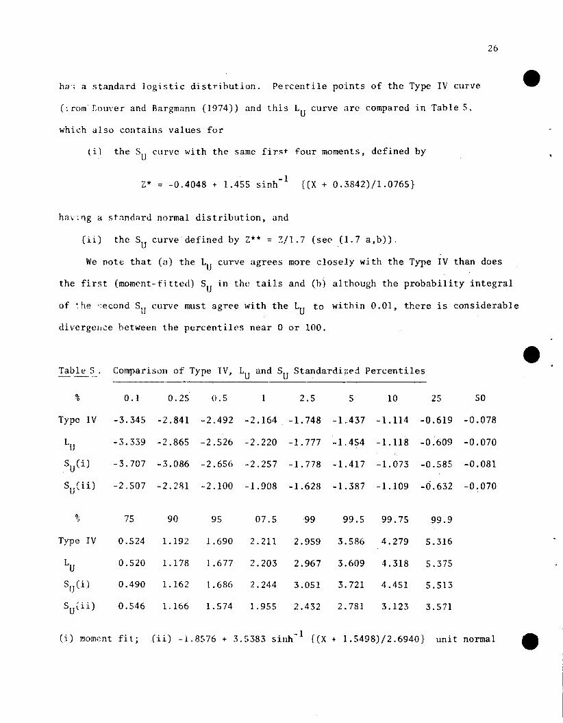
ha; a standard logistic distribution. Percentile points of the Type IV curve

C;romf,ouver and Bargmann (1974)) and this LU

curve are compared in TableS,

which also contains values for

ti) the Su curve with the same fi rc;;'t four moments, defined by

Z* = -0.4048 + 1.455 sinh- l {(X + 0.3842)/1.0765)

having a standard normal distribution, and

(ii) the Su curve-defined by Z** = Z/I.7 (see (1.7 a,b)).

We note that (a) the LU curve agrees more closely with the Type IV than does

the fi rst (moment- fj tted) Sv in the tails and (b) although the probabiIity integral

of ~he <~econd Su curve must agree with the Lu to within 0.01, there is considerable

di vergellce between the percentiles near 0 or 100.

Table 5 . Comparison of Type IV, LU and Su Standardii:ed Percentiles

% o. ] 0.25 0.5 1 2.5 5 10 2S 50

Type IV -3.345 -2.841 -2.492 -2.164 -1. 748 -1 .. 437 -1.114 -0.619 -0.078

LU -3.339 -2.865 -2.526 -2.220 -1.777 -1..454 -1.118 -0.609 -0.070

SU(i) -3.707 -3.086 -2.656 -2.257 -1.778 -1.417 -1.073 -0.585 -0.081

S ( .. ) -2.507 - 2.281 -2.100 -1. 908 -1.628 -1. 387 -1.109 -0.632 -0.0701J,11

% 75 90 95 07.5 99 99.5 99.75 99.9

Type IV 0.524 1.192 1.690 2.211 2.959 3.586 4.279 5.316

LV 0.520 1.178 1.677 2.203 2.967 3.609 4.318 5.375

SUCi) 0.490 1.162 1.686 2.244 3.051 3.721 4.451 5.513

SUCii) 0.546 1.166 1.574 1.955 2.432 2.781 3.123 3.571

(i) moment fit; (ii) -1.8576 + 3.5383 sinh- l {eX + 1.5498)/2.6940} unit normal

()

1

2

3

4

5

6

7

8

9

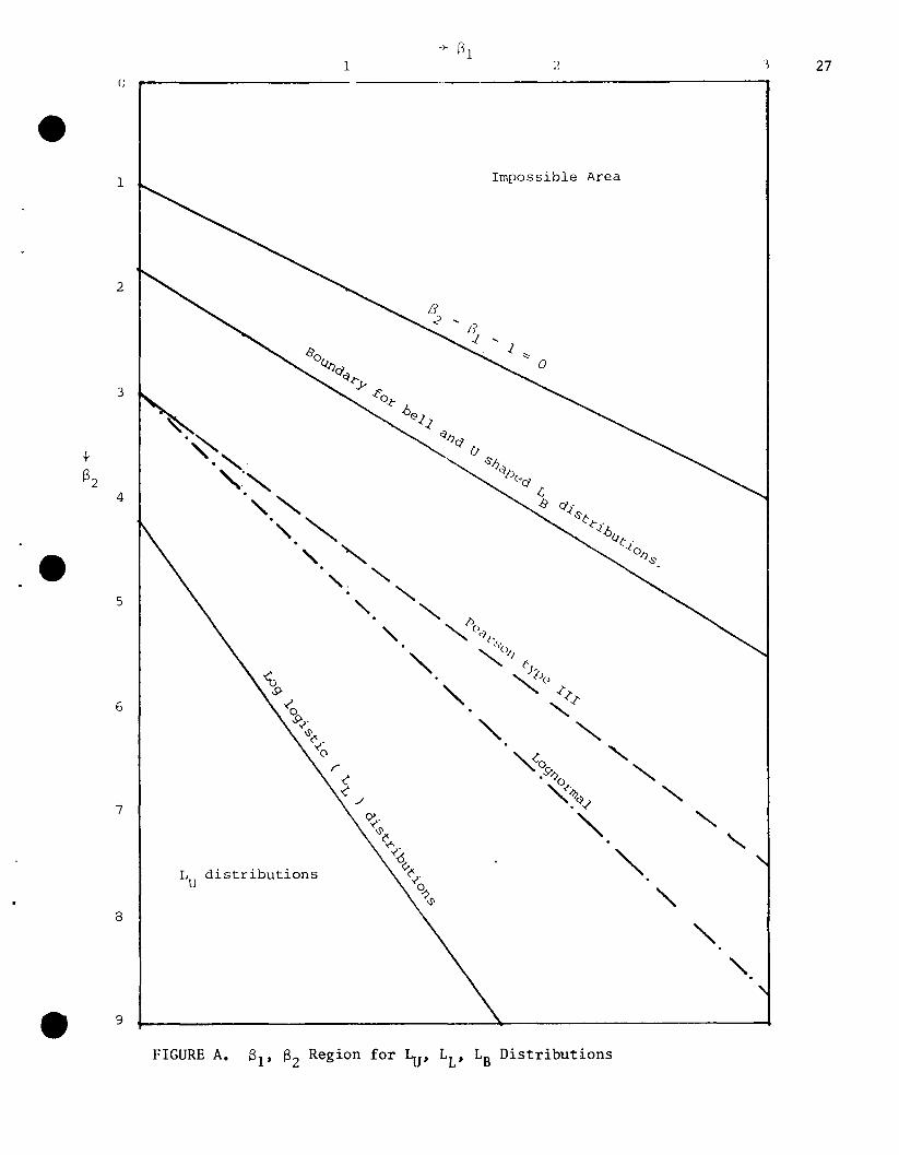
>- G11

Impossible Area

LU

distributions

FIGURE A. Sl' S2 Region for LU' LL' LB Distributions

1 27

28

References

Bouver, H. and Bargmann, R.E. (1974), "Tables of the standardized percentage points

of the Pearson system in terms of ~\ and 132

" THE'MIS Tech. Rep. 32, Department

of Statistics, University of Georgia.

Brown, K.M. (1967), "Solution of simultaneous nonlinear equations", COrmi. ACM, 10,

728-729.

vBukac, J. (1972), "Fitting SB curves using synunetrica1 percentile points",

Biometrika, 59, 688-690.

Burr, I.W. (1942), "Cumulative frequency functions", Ann. Math. Statist., 13,

215-232.

Dubey, S. D. (1966), "Transformations for estimation of parameters", J. Ind. Statist.

Assoc., 4, 109-124.

Hahn, G. J. and Shapiro, S. (1967), Statistical Models in Engineering, New York: Wiley.

Johnson, N.L. (1949), "Systems of frequency curves generated by methods of trans1a- etion", Biometl'ika, 36, 149-176.

Johnson, N.L. (1954), "Systems of frequency curves derived from the first law of

Laplace", Trul}. Estad., 5, 283-291.

Johnson, N.L. and Kotz, S. (1970), Distributions in Statistics: Continous Univariate

Distributions, 2, New York: Wiley.

Lomax, K.S. (1954), "Business failures: Another example of the analysis of failure

data", J. Amer. Statist. Assoc., 49, 847-852.

Mage, D.T. (1979), "An explicit solution for SB parameters using four percentile

points", Technometrics.

Pearson, E. S., Johnson, N. L., and Burr, 1. W. (1979), "Comparisons of the percentage

points of distributions with the same first four moments, chosen from eight

different systems of frequency curves", COrmi. Statist., BB, 191-229.

•

29

e Pearson, E.S. and Hartley, H.O. (Eds.)(1976), Biometrika Tables for Statisticians,

2, Cambridge University Press.

Shah, B. K. and Dave, P .H. (1963), "A note on long-logistic distribution", J. of

M.S. Univ. Boroda (Sen. Number)~ 12, 21-22.

Slifker, .J.F. and Shapiro, 5.5. (1979), "On the Johnson system of distributions",

Technometrics .