Embed Size (px)
Citation preview
Chapter 2
The Finite Element Method Kelly 31
2 The (Galerkin) Finite Element Method
2.1 Approximate Solution and Nodal Values
In order to obtain a numerical solution to a differential equation using the Galerkin Finite
Element Method (GFEM), the domain is subdivided into finite elements. The function is
approximated by piecewise trial functions over each of these elements. This is illustrated
below for the one-dimensional case, with linear functions used over each element, p being
the dependent variable.
Figure 2.1: A mesh of N one dimensional Finite Elements
nodes elements
true solution approximating
functions
element i node
i
node
i+1
ip
1ip
ip
1ip
Chapter 2
The Finite Element Method Kelly 32
The unknowns of the problem are the nodal values of p, ip 11 Ni , at the element
boundaries (which in the 1D case are simply points). The (approximate) solution within
each element can then be constructed once these nodal values are known.
2.2 Trial Functions
2.2.1 Lagrange and Hermite Elements
There are an endless number of different trial functions which one can use. In practice,
these trial functions can be grouped into two broad types. The first consists of the
Lagrange or 0C trial functions (and corresponding Lagrange or 0C element). These are
trial functions which are continuous across element boundaries, but whose first derivatives
are not continuous across boundaries. The elements in Fig. 2.1 are 0C linear elements –
there is a clear jump in the first derivative of the trial functions at the element boundaries
(nodes) – the first derivative is piecewise continuous.
The second group consists of the Hermite or 1C trial functions (elements). These are
functions which are not only continuous across element boundaries, but whose first
derivatives are also continuous across boundaries.
In general, a nC element is one for which the trial functions are continuous up to the thn
derivative, but elements with 1n are rarely used. In fact, three of the most commonly
encountered types of element are those with a
(1) linear Lagrange trial function ( 0C )
(2) quadratic Lagrange trial function ( 0C )
(3) cubic Hermite trial function ( 1C )
These three trial functions / elements will be discussed in what follows.
Obviously, the higher the order and the higher the continuity of the element, the better the
accuracy one would expect, but the more computation which is required.
2.2.2 The C0 Linear Element
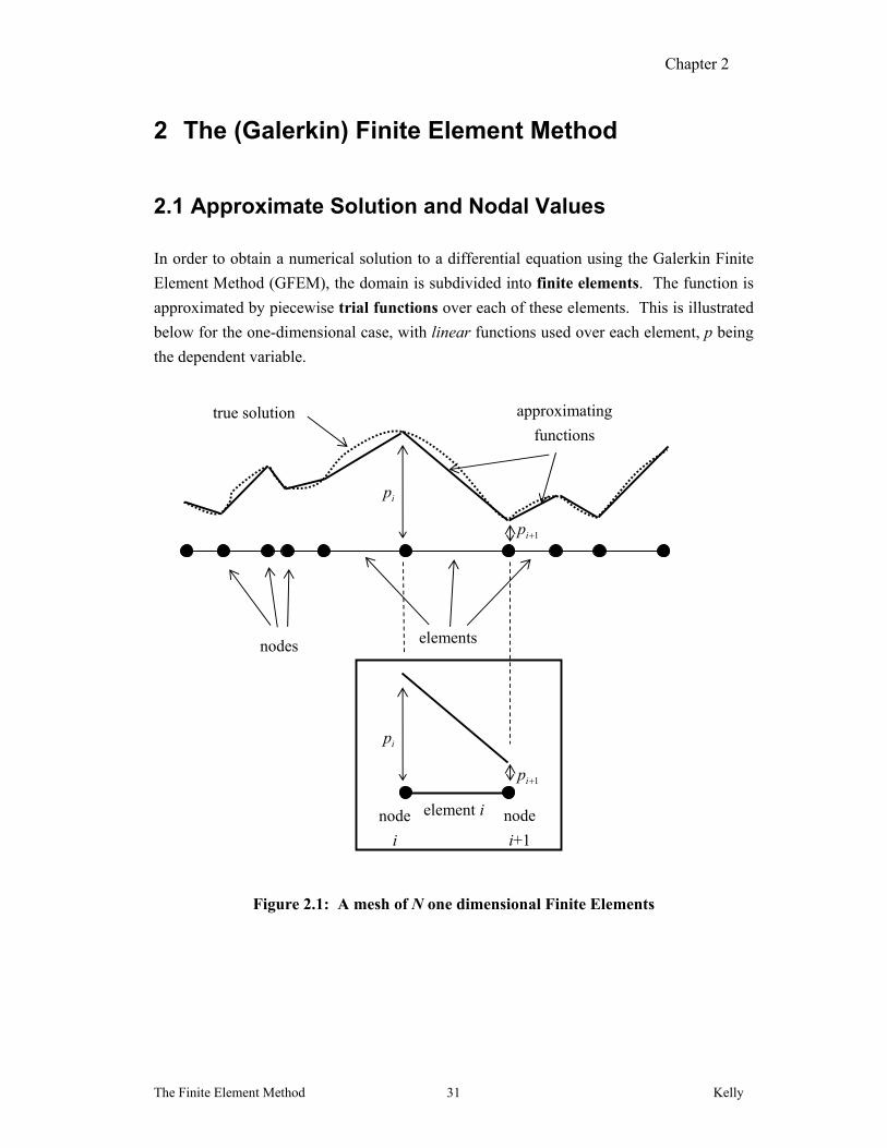
The 0C linear element is by far the most commonly used finite element. Consider one typical element of the domain, with end-points 21, xx , Fig. 2.2. Assuming a linear
interpolation,
Chapter 2
The Finite Element Method Kelly 33
bxaxp )(~ . (2.1)
Let the (unknown) end-point values be 2211
~)(~,~)(~ pxppxp . This gives two algebraic
equations in two unknowns a and b,
22
11
~
~
bxap
bxap
(2.2)
Solving the equations gives
12
12
12
1221~~
,~~
xx
ppb
xx
xpxpa
(2.3)
so that, after some algebra, one can write ( )p x in terms of the two unknowns 1 2,p p
(instead of in the form of Eqn. 2.1, which is in terms of the two values a and b)
Linear Trial Function:
L
xxxN
L
xxxN
pxNpxNxp
12
21
2211
)(,)(
~)(~)()(~
(2.4)
where L is the length of the element, 12 xxL .
Figure 2.2: Linear trial function approximation over an element
1x 2x
linear trial
function
22~)(~ pxp
11~)(~ pxp
true
solution
nodal points
Chapter 2
The Finite Element Method Kelly 34
The function )(xp can now be approximated over each interval through
1121
323221
212211
,~)(~)(
,~)(~)(,~)(~)(
)(~
NNNN xxxpxNpxN
xxxpxNpxNxxxpxNpxN
xp (2.5)
Here, the shape (or basis) functions 21 , NN are the same over each interval (although
they don’t have to be – they could be interspersed with, for example, quadratic shape
functions – see later).
Structure of the Linear Shape Functions
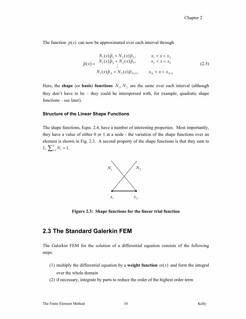
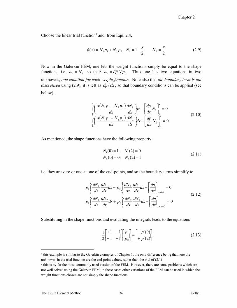
The shape functions, Eqns. 2.4, have a number of interesting properties. Most importantly,
they have a value of either 0 or 1 at a node - the variation of the shape functions over an
element is shown in Fig. 2.3. A second property of the shape functions is that they sum to
1, 12
1 i iN .
Figure 2.3: Shape functions for the linear trial function
2.3 The Standard Galerkin FEM
The Galerkin FEM for the solution of a differential equation consists of the following
steps:
(1) multiply the differential equation by a weight function )(x and form the integral
over the whole domain
(2) if necessary, integrate by parts to reduce the order of the highest order term
1x 2x
1N 2N
Chapter 2
The Finite Element Method Kelly 35
(3) choose the order of interpolation (e.g. linear, quadratic, etc.) and corresponding
shape functions miNi 1, , with trial function
m
i ii pxNxpp1
)()(~
(4) evaluate all integrals over each element, either exactly or numerically, to set up a system of equations in the unknown ip ’s
(5) solve the system of equations for the ip ’s.
The linear 0C element will be used in what follows. Quadratic and cubic elements will be
considered later.
2.3.1 A Single-Element Example
Consider the following problem: solve the following differential equation using one linear
element:
0)2(,1)0(,02
2
ppdx
pd (2.6)
[the exact solution is 2)( xxp ]
First, multiply the equation across by )(x and integrating over 2,0 to get the weighted
residual integral
0)(2
02
2
dxx
dx
pdI (2.7)
Integrating by parts (and multiplying across by 1 ) leads to the weak form
02
0
2
0
dx
dpdx
dx
d
dx
dpI . (2.8)
This step is crucial to the FEM when linear trial functions are used, since if the trial function p~ is linear, then 0~ p , and one cannot work with (2.7). However, by first
integrating by parts, there is no longer any second derivative and (2.8) is no longer the
trivial 00 .
Chapter 2
The Finite Element Method Kelly 36
Choose the linear trial function1 and, from Eqn. 2.4,
2211)(~ pNpNxp 2
11
xN
22
xN (2.9)
Now in the Galerkin FEM, one lets the weight functions simply be equal to the shape functions, i.e. ii N , so that2 ii pp /~ . Thus one has two equations in two
unknowns, one equation for each weight function. Note also that the boundary term is not discretised using (2.9), it is left as dxdp / , so that boundary conditions can be applied (see
below),
0
0
2
02
2
0
22211
2
01
2
0
12211
Ndx
dpdx
dx
dN
dx
pNpNd
Ndx
dpdx
dx
dN
dx
pNpNd
(2.10)
As mentioned, the shape functions have the following property:
1 1
2 2
(0) 1, (2) 0
(0) 0, (2) 1
N N
N N
(2.11)
i.e. they are zero or one at one of the end-points, and so the boundary terms simplify to
0
0
2 node
2
0
222
2
0
211
1 node
2
0
122
2
0
111
dx
dpdx
dx
dN
dx
dNpdx
dx
dN
dx
dNp
dx
dpdx
dx
dN
dx
dNpdx
dx
dN
dx
dNp
(2.12)
Substituting in the shape functions and evaluating the integrals leads to the equations
)2(
)0(
11
11
2
1
2
1
p
p
p
p (2.13)
1 this example is similar to the Galerkin examples of Chapter 1, the only difference being that here the
unknowns in the trial function are the end-point values, rather than the a, b of (2.1) 2 this is by far the most commonly used version of the FEM. However, there are some problems which are
not well solved using the Galerkin FEM; in these cases other variations of the FEM can be used in which the
weight functions chosen are not simply the shape functions
Chapter 2
The Finite Element Method Kelly 37
Applying the essential boundary condition 0)2( p , the first equation with the natural BC
(0) 1p gives 21)0( 1121 ppp . From the second equation, one finds that
1)2( p . The full solution is
2)2/(2/1 21 xpxpxp (2.14)
Note that the solution is exact – because the solution was assumed to be linear, and it is.
Consider now the general ordinary differential equation with constant coefficients:
dcudx
dub
dx
uda
2
2
(2.15)
The weighted residual integral is
02
1
2
1
2
1
x
x
x
x
x
x dx
duadxddxcu
dx
dub
dx
d
dx
duaI
. (2.16)
Using the linear trial function, and after some algebra, one arrives at the system of two
equations
Equations for Linear Trial Function:
)(
)(
1
1
2~
~
21
12
611
11
2
1
11
111
2
1
2
1
xu
xua
Ld
u
uLcb
La (2.17)
As an example, let 1,2,1 dcba and 1,1,0 21 Lxx . The exact solution for
the boundary conditions 2)(,1~)( 211 xuuxu is 11)( xxexu . Putting these values
directly into the linear equations Eqn. 2.17 immediately yields 2.2~2 u and 2.0)( 1 xu
(compared with the exact solutions 2 and 0.368 respectively) so
xxuxuxu 2.11~1~)(~
21 (2.18)
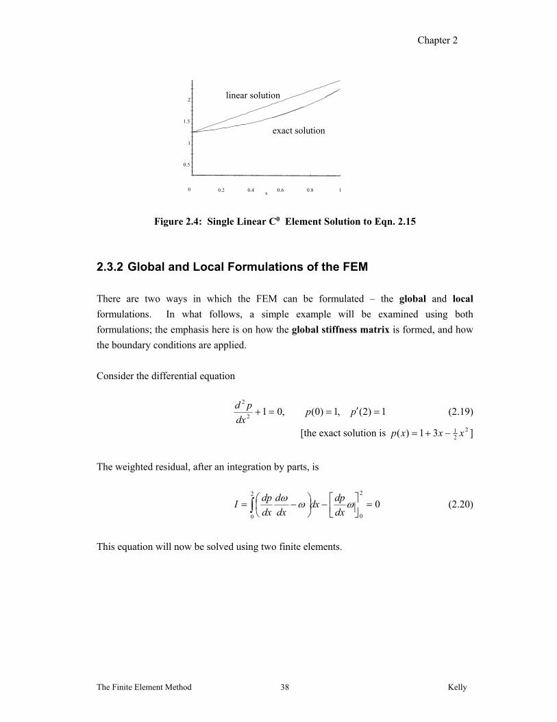
This solution is compared with the exact solution in Fig. 2.4.
Chapter 2
The Finite Element Method Kelly 38
Figure 2.4: Single Linear C0 Element Solution to Eqn. 2.15
2.3.2 Global and Local Formulations of the FEM
There are two ways in which the FEM can be formulated – the global and local
formulations. In what follows, a simple example will be examined using both
formulations; the emphasis here is on how the global stiffness matrix is formed, and how
the boundary conditions are applied.
Consider the differential equation
1)2(,1)0(,012
2
ppdx
pd (2.19)
[the exact solution is 22131)( xxxp ]
The weighted residual, after an integration by parts, is
02
0
2
0
dx
dpdx
dx
d
dx
dpI (2.20)
This equation will now be solved using two finite elements.
0
0.5
1
1.5
2
0.2 0.4 0.6 0.8 1x
linear solution
exact solution
Chapter 2
The Finite Element Method Kelly 39
Solution: The Global Formulation
In the global formulation, one uses a single trial function which extends over the complete
domain3,
332211 )(~
)(~
)(~
)(~ pxNpxNpxNxp (2.21)
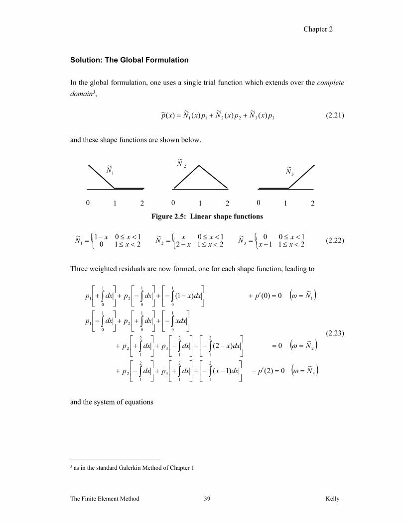
and these shape functions are shown below.
Figure 2.5: Linear shape functions
211
100~21210~
210101~
321 xxxNxx
xxNxxxN (2.22)
Three weighted residuals are now formed, one for each shape function, leading to
3
2
1
2
1
3
2
1
2
2
2
1
2
1
3
2
1
2
1
0
1
0
2
1
0
1
1
1
0
1
0
2
1
0
1
~0)2()1(
~0)2(
~0)0()1(
Npdxxdxpdxp
Ndxxdxpdxp
xdxdxpdxp
Npdxxdxpdxp
(2.23)
and the system of equations
3 as in the standard Galerkin Method of Chapter 1
1 0 2 1 0 2 1 0 2
1
~N
2
~N
3
~N
Chapter 2
The Finite Element Method Kelly 40
)2(
1
)0(
110
121
011
21
21
3
2
1
p
p
p
p
p
(2.24)
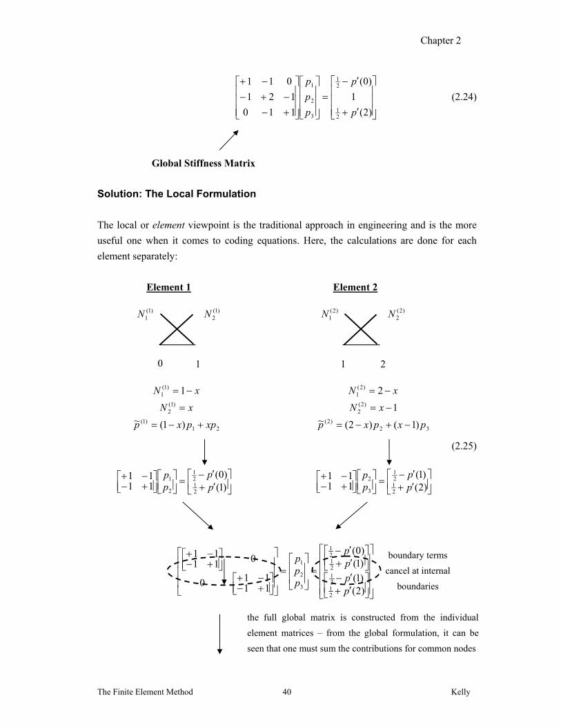
Solution: The Local Formulation
The local or element viewpoint is the traditional approach in engineering and is the more
useful one when it comes to coding equations. Here, the calculations are done for each
element separately:
Element 1 Element 2
(2.25)
)1()0(
1111
2121
2
1
pp
pp
)2()1(
1111
2121
3
2
pp
pp
1 0
)1(1N
21)1(
)1(2
)1(1
)1(~
1
xppxp
xN
xN
)1(2N
2 1
)2(1N
32)2(
)2(2
)2(1
)1()2(~1
2
pxpxp
xN
xN
)2(2N
boundary terms
cancel at internal
boundaries
)2()1(
)1()0(
11110
01111
21212121
3
2
1
pp
pp
ppp
Global Stiffness Matrix
the full global matrix is constructed from the individual
element matrices – from the global formulation, it can be
seen that one must sum the contributions for common nodes

Chapter 2
The Finite Element Method Kelly 41
)2(
1
)0(
110
121
011
21
21
3
2
1
p
p
p
p
p
Boundary Conditions
Apply now the BC’s 1)2(,1)0( pp to get
21
223
3
2 )0(,2
11
12
ppp
p (2.26)
which can be solved for
3)0(,5, 32
72 ppp (2.27)
The solution here happens to be exact at the nodes – this will be the case for problems of the form )(xfp .
Returning now to the trial functions (2.21) or (2.25), the full solution, graphed in Fig. 2.6,
is
Element 1: xp 2
5)1( 1~
Element 2: xp 23)2( 2~
Note that, when programming the FE, it is best if rows and columns of the coefficient
matrix are not eliminated as in going from (2.24) to (2.26), when applying boundary
conditions. The essential BC corresponds to node 1, so we replace the first row with the
essential BC. If one wants to preserve a symmetric coefficient matrix, one can also then
replace the first column with zeros (and a 1). In this way, application of the boundary
conditions to the above system of 3 equations would lead to (note how the “ 1 ” in the first
column, second row, of the original coefficient matrix, is brought over to the right hand
side, changing the 1 to a 2)
Chapter 2
The Finite Element Method Kelly 42
23
3
2
1
2
1
110
120
001
p
p
p
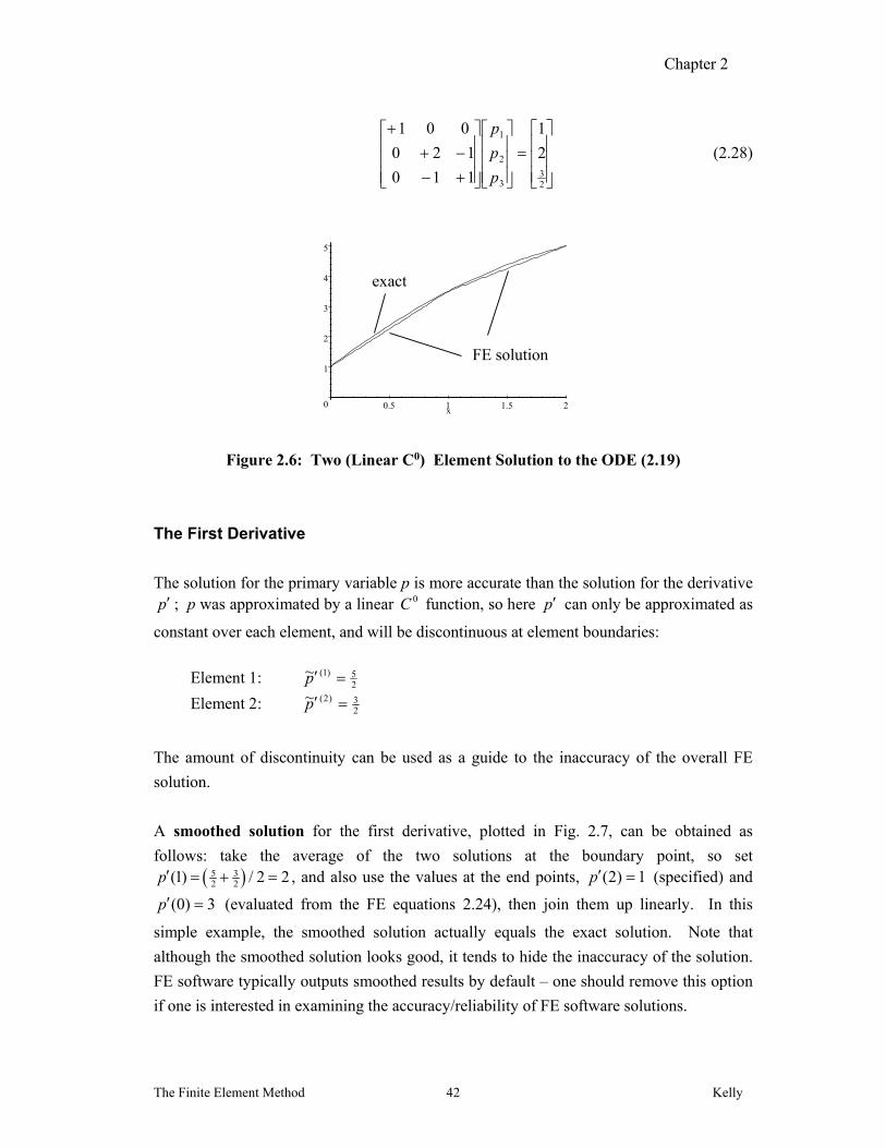
(2.28)
Figure 2.6: Two (Linear C0) Element Solution to the ODE (2.19)
The First Derivative
The solution for the primary variable p is more accurate than the solution for the derivative p ; p was approximated by a linear 0C function, so here p can only be approximated as
constant over each element, and will be discontinuous at element boundaries:
Element 1: 2
5)1(~ p
Element 2: 23)2(~ p
The amount of discontinuity can be used as a guide to the inaccuracy of the overall FE
solution.
A smoothed solution for the first derivative, plotted in Fig. 2.7, can be obtained as
follows: take the average of the two solutions at the boundary point, so set 5 3
2 2(1) / 2 2p , and also use the values at the end points, 1)2( p (specified) and
3)0( p (evaluated from the FE equations 2.24), then join them up linearly. In this
simple example, the smoothed solution actually equals the exact solution. Note that
although the smoothed solution looks good, it tends to hide the inaccuracy of the solution.
FE software typically outputs smoothed results by default – one should remove this option
if one is interested in examining the accuracy/reliability of FE software solutions.
0
1
2
3
4
5
0.5 1 1.5 2x
exact
FE solution
Chapter 2
The Finite Element Method Kelly 43
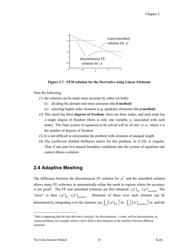
Figure 2.7: FEM solution for the Derivative using Linear Elements
Note the following:
(1) the solution can be made more accurate by either (or both)
(i) dividing the domain into more elements (the h-method)
(ii) selecting higher order elements (e.g. quadratic elements) (the p-method)
(2) This mesh has three degrees of freedom: there are three nodes, and each node has
a single degree of freedom (there is only one variable, p, associated with each
node). The final system of equations to be solved will be of size nn , where n is
the number of degrees of freedom.
(3) It is not difficult to reformulate the problem with elements of unequal length
(4) The coefficient (Global Stiffness) matrix for this problem, in (2.24), is singular.
Thus if one puts two natural boundary conditions into the system of equations one
cannot obtain a solution.
2.4 Adaptive Meshing The difference between the discontinuous FE solution for p and the smoothed solution
allows many FE softwares to automatically refine the mesh in regions where the accuracy is not good4. The FE and smoothed solutions are first obtained: FE smoothed
,p p . The
“error” is then FE smoothedp p . Measures of these over each element can be
determined by integrating over the element, say 2
FEiL
p dx , 2
smoothediL
p dx and the
4 that is supposing that the first derivative shouldn’t be discontinuous – it may well be discontinuous, in
certain problems, for example where a stress field is discontinuous at the interface between different
materials
0
0.5
1
1.5
2
2.5
3
0.5 1 1.5 2x
exact/smoothed solution for p
discontinuous FE solution for p
Chapter 2
The Finite Element Method Kelly 44
element error (squared) 2
FE smoothedi
i Le p p dx . An example of a global relative
error would then be
2
FEi
i
iL
e
p dx e
(2.29)
is a global parameter – it doesn’t measure error at a particular point/element (element
mesh-adaptation parameters might be unreliable, since they would be large simply if
2
FEiL
p dx were small). An algorithm might then be: evaluate ; if 05.0
terminate, otherwise refine the mesh in regions where ie is large; stop after, say, 5
iterations. Note that neither nor e can reveal the percentage error in the analysis, since
the true solution is unknown.
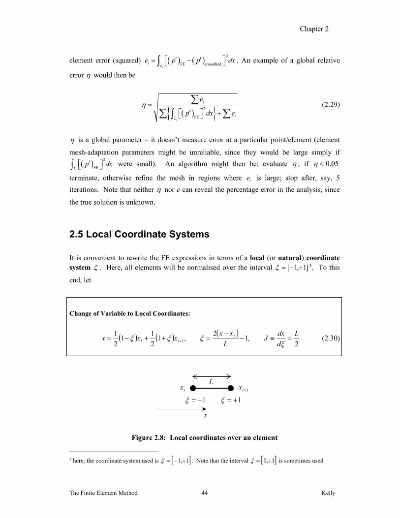
2.5 Local Coordinate Systems
It is convenient to rewrite the FE expressions in terms of a local (or natural) coordinate system . Here, all elements will be normalised over the interval ]1,1[ 5. To this
end, let
Change of Variable to Local Coordinates:
2
,12
,12
11
2
11
L
d
dxJ
L
xxxxx i
ii
(2.30)
Figure 2.8: Local coordinates over an element
5 here, the coordinate system used is 1,1 . Note that the interval 1,0 is sometimes used
L
1ix 1ix
x
1
Chapter 2
The Finite Element Method Kelly 45
From Eqn. 2.4,
Linear Shape Functions (Local Coordinates)
12
1,1
2
121 NN (2.31)
This change of coordinates results in integrals which appear again and again in different
FE problems, and they only have to be evaluated on a once-and-for-all basis. A number of
this type of important integral are evaluated in the Appendix to this chapter. In higher
dimensional problems (2-D and 3-D), this normalisation allows one to obtain approximate
solutions to the integrals using numerical integration rules.
As an example of using the local coordinate system, consider this problem: solve the
following differential equation using two linear elements of equal length:
2,1)1(,122
2
xdx
dppdx
dp
dx
pd (2.32)
[the exact solution is xexexp 2)( ]
One has
02
1
2
1
dx
dpdxw
dx
dp
dx
d
dx
dpI . (2.33)
In the global coordinate system,
Element 1: )1(1
0
)1(
0
)1()1(2
10
)1()1(2
1
pdxNdxNdx
dNpdx
dx
dN
dx
dNp j
L
j
L
ji
ii
Lji
ii
Element 2: )2(2
2)2(
2)2(
)2(1
2
11
2 )2()2(1
2
11 pdxNdxN
dx
dNpdx
dx
dN
dx
dNp j
L
L
j
L
L
ji
i
L
L
j
ii
(2.34)
with 2,1j . Changing to local coordinates, note first the shape functions,
Chapter 2
The Finite Element Method Kelly 46
Element 1: 2
)1(
1
)1(
2)1(
21)1(
1)1(
2
1
2
1pppNpNp
12 1)1(
Lx
Element 2: 3
)2(
2
)2(
3)2(
22)2(
1)2(
2
1
2
1pppNpNp
12 2/3)2(
Lx
(2.35)
with 2
1L . Using the chain rule, / / /dN dx dN d d dx and, from Eqn. 2.30,
/ 2 /d dx L , this leads to
)2(2
2
)1(2
2
2
1
1
2
1
1
1
1
1
1
1
1
2
1
1
1
1
1
pdNL
dNd
dNd
d
dN
d
dN
Lp
pdNL
dNd
dNd
d
dN
d
dN
Lp
jji
jiji
i
jji
jiji
i
(2.36)
The square bracketed terms/integrals are evaluated in the Appendix to this Chapter so that
Element 1: 0
0)1(
41
223
123
41
225
125
pp
ppp
Element 2: 0)2(
0
41
323
223
41
325
225
ppp
pp
and the following system of three equations is obtained:
)2(
)1(
0
4
0
41
21
41
3
2
1
23
23
25
23
25
25
p
p
p
p
p
(2.37)
The essential boundary condition is applied at 1 and the natural boundary condition at 2,
which leads to
7777.3
6111.214
934
1847
3
2
47
3
2
23
23
25
p
p
p
p (2.38)
Chapter 2
The Finite Element Method Kelly 47
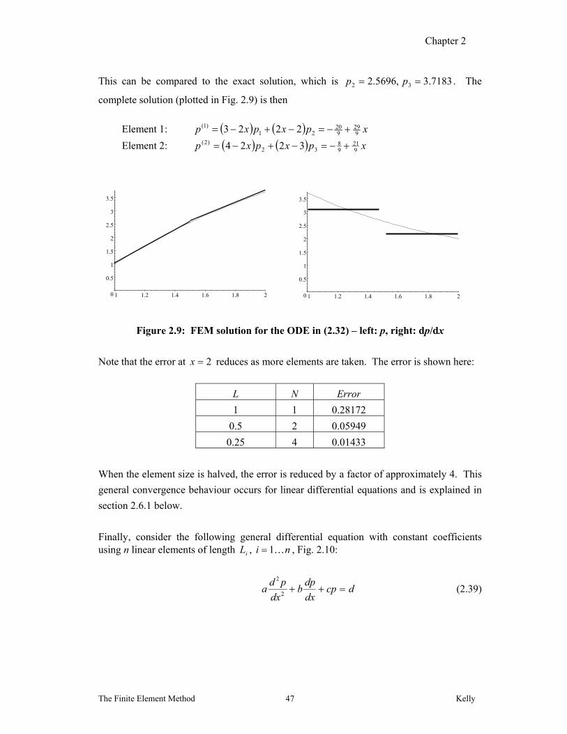
This can be compared to the exact solution, which is 7183.3,5696.2 32 pp . The
complete solution (plotted in Fig. 2.9) is then
Element 1: xpxpxp 9
29920
21)1( 2223
Element 2: xpxpxp 921
98
32)2( 3224
Figure 2.9: FEM solution for the ODE in (2.32) – left: p, right: dp/dx
Note that the error at 2x reduces as more elements are taken. The error is shown here:
L N Error
1 1 0.28172
0.5 2 0.05949
0.25 4 0.01433
When the element size is halved, the error is reduced by a factor of approximately 4. This
general convergence behaviour occurs for linear differential equations and is explained in
section 2.6.1 below.
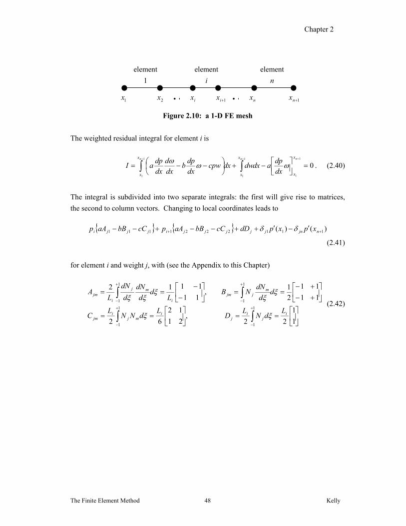
Finally, consider the following general differential equation with constant coefficients using n linear elements of length iL , ni 1 , Fig. 2.10:
dcpdx
dpb
dx
pda
2
2
(2.39)
0
0.5
1
1.5
2
2.5
3
3.5
1 1.2 1.4 1.6 1.8 2 0
0.5
1
1.5
2
2.5
3
3.5
1 1.2 1.4 1.6 1.8 2
Chapter 2
The Finite Element Method Kelly 48
Figure 2.10: a 1-D FE mesh
The weighted residual integral for element i is
01
1
1
1
1
1
nnn x
x
x
x
x
x dx
dpadxdwdxcpw
dx
dpb
dx
d
dx
dpaI
. (2.40)
The integral is subdivided into two separate integrals: the first will give rise to matrices,
the second to column vectors. Changing to local coordinates leads to
)()( 1112221111 njnjjjjjijjji xpxpdDcCbBaApcCbBaAp
(2.41)
for element i and weight j, with (see the Appendix to this Chapter)
1
1
22,
21
12
62
11
11
2
1,
11
1112
1
1
1
1
1
1
1
1
ij
ij
imj
ijm
mjjm
i
mj
ijm
LdN
LD
LdNN
LC
dd
dNNB
Ld
d
dN
d
dN
LA
(2.42)
1x 2x ix 1ix nx 1nx
element
i
element
n
element
1
Chapter 2
The Finite Element Method Kelly 49
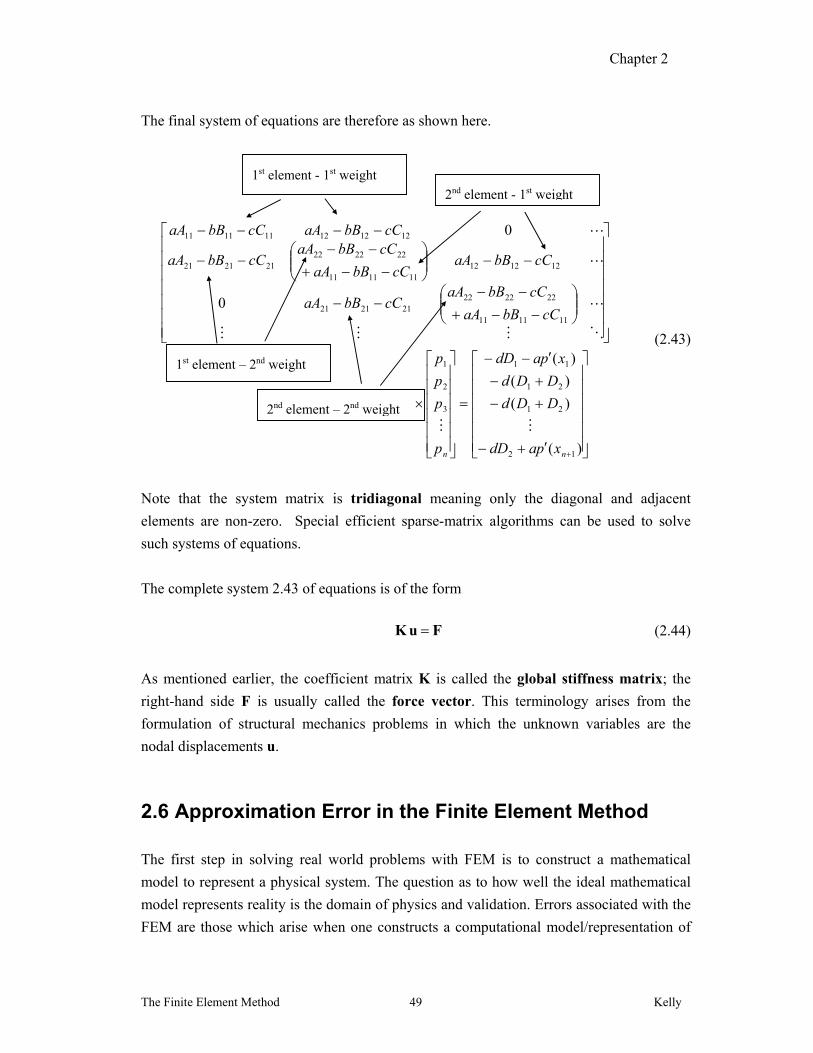
The final system of equations are therefore as shown here.
)(
)(
)(
)(
0
0
12
21
21
11
3
2
1
111111
222222212121
121212111111
222222212121
121212111111
nn xpadD
DDd
DDd
xpadD
p
p
p
p
cCbBaA
cCbBaAcCbBaA
cCbBaAcCbBaA
cCbBaAcCbBaA
cCbBaAcCbBaA
(2.43)
Note that the system matrix is tridiagonal meaning only the diagonal and adjacent
elements are non-zero. Special efficient sparse-matrix algorithms can be used to solve
such systems of equations.
The complete system 2.43 of equations is of the form
K u F (2.44)
As mentioned earlier, the coefficient matrix K is called the global stiffness matrix; the
right-hand side F is usually called the force vector. This terminology arises from the
formulation of structural mechanics problems in which the unknown variables are the
nodal displacements u.
2.6 Approximation Error in the Finite Element Method
The first step in solving real world problems with FEM is to construct a mathematical
model to represent a physical system. The question as to how well the ideal mathematical
model represents reality is the domain of physics and validation. Errors associated with the
FEM are those which arise when one constructs a computational model/representation of
1st element - 1st weight
2nd element - 1st weight
1st element – 2nd weight
2nd element – 2nd weight
Chapter 2
The Finite Element Method Kelly 50
the mathematical model and solve that computational model. Apart from bugs in software
and “mistakes” made by the user, the main sources of error in the FEM are discretization
error and solution error.
The discretization error arises when the mathematical model is converted into a discrete
computational model. It is the error introduced when representing a function of a
continuous variable by its values at a discrete set of nodes; or, equivalently, when
representing a differential equation by its FEM matrix equations. This error will depend on
the element order (linear, quadratic, etc.) and also on the number of elements used to
represent the domain of interest. One would expect that the discretization error will tend to
zero as the mesh of elements is made smaller by reducing element size.
The discretization error is associated with the complete problem and so is a global
measure. The discretization error itself depends on the more local element level on the
interpolation error. This is the error which arises when a function is approximated using
shape functions over a particular element, and is discussed further below6.
Other errors which can arise are those associated with numerical integration (all integrals
are evaluated exactly in this chapter, but only approximate values can be obtained in higher
dimensions), and numerical/rounding errors, for example in inverting the stiffness K
matrix.
2.6.1 Interpolation Error
The interpolation error is usually the largest source of error in the FEM. It can be
calculated for any typical element; for example, with the linear element, one can proceed
as follows:
The FE approximation is given by
2211 )()()(~ pNpNp (2.45)
6 One is most often interested in the interpolation error for functions; one can also examine the interpolation
errors associated with the gradients of functions
Chapter 2
The Finite Element Method Kelly 51
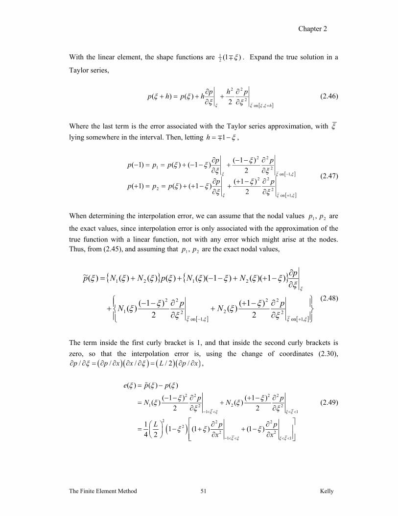
With the linear element, the shape functions are 12 (1 ) . Expand the true solution in a
Taylor series,
h
phphphp
,on
2
22
2)()( (2.46)
Where the last term is the error associated with the Taylor series approximation, with
lying somewhere in the interval. Then, letting 1h ,
,1on 2
22
2
,1on 2
22
1
2
)1()1()()1(
2
)1()1()()1(
ppppp
ppppp
(2.47)
When determining the interpolation error, we can assume that the nodal values 21 , pp are
the exact values, since interpolation error is only associated with the approximation of the
true function with a linear function, not with any error which might arise at the nodes. Thus, from (2.45), and assuming that 21 , pp are the exact nodal values,
,1on 2
22
2
,1on 2
22
1
2121
2
)1()(
2
)1()(
)1)(()1)(()()()()(~
pN
pN
pNNpNNp
(2.48)
The term inside the first curly bracket is 1, and that inside the second curly brackets is
zero, so that the interpolation error is, using the change of coordinates (2.30), / / / / 2 /p p x x L p x ,
2 2 2 2
1 22 2
1 1
2 2 22
2 2
1 1
( ) ( ) ( )
( 1 ) ( 1 )( ) ( )
2 2
11 (1 ) (1 )
4 2
e p p
p pN N
L p p
x x
(2.49)
Chapter 2
The Finite Element Method Kelly 52
The maximum error in the element is then
2 2 2
2 20-1 1
2 2
2
1 116
Max8
L p pe
x x
L p
x
(2.50)
Thus as the length of the element is decreased, the error decreases as the square of the
element length. One says that the linear element is second-order accurate:
2Le (2.51)
In general, the error of an element is proportional to 1kL , where L is the length, or a
characteristic length, of the element, and k is the order of the interpolating polynomial.
The error in the first derivative is proportional to kL .
The same applies, to a certain extent, for higher dimensions. For example, the error for a
linear 2-D triangular element is proportional to 2l , where l is a characteristic length of the
element.
2.7 Quadratic C0 Elements
Here the 0C quadratic trial function is examined.
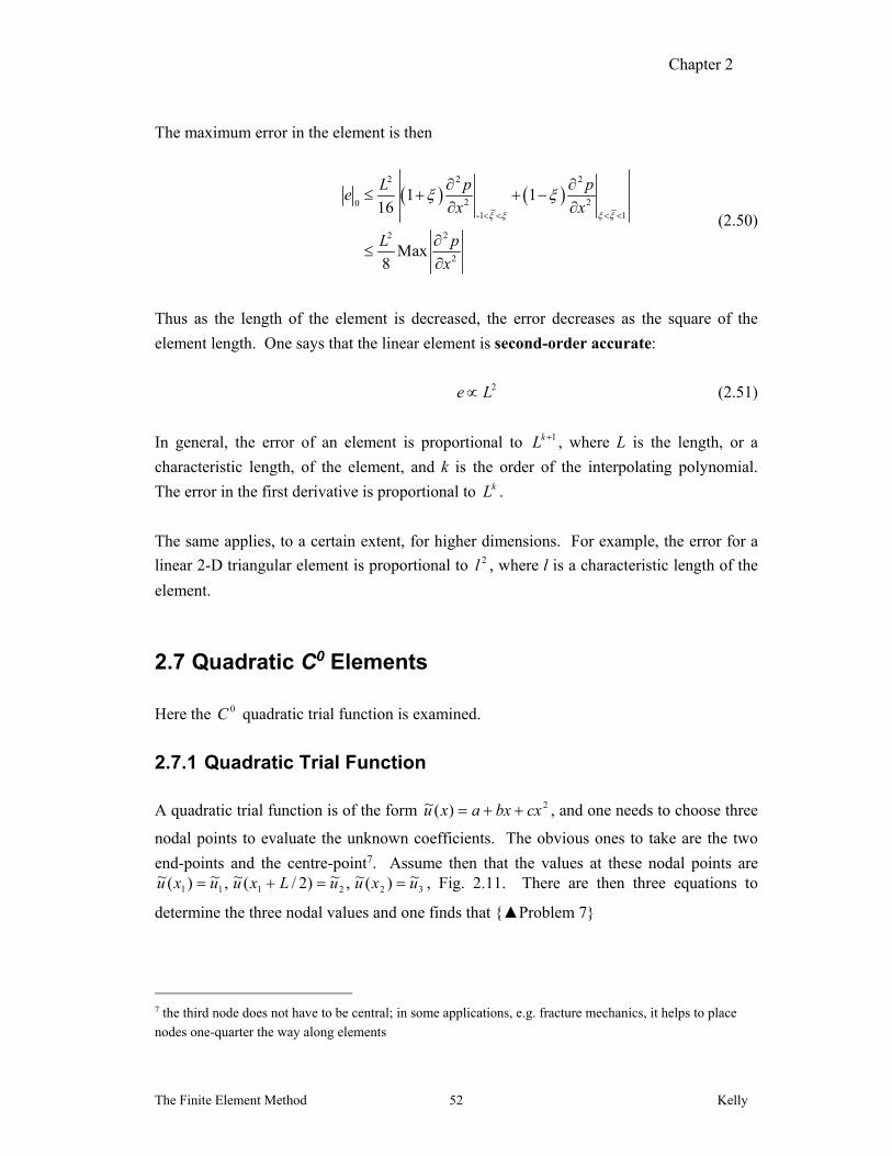
2.7.1 Quadratic Trial Function A quadratic trial function is of the form 2)(~ cxbxaxu , and one needs to choose three
nodal points to evaluate the unknown coefficients. The obvious ones to take are the two
end-points and the centre-point7. Assume then that the values at these nodal points are
322111~)(~,~)2/(~,~)(~ uxuuLxuuxu , Fig. 2.11. There are then three equations to
determine the three nodal values and one finds that {▲Problem 7}
7 the third node does not have to be central; in some applications, e.g. fracture mechanics, it helps to place
nodes one-quarter the way along elements
Chapter 2
The Finite Element Method Kelly 53
Quadratic Trial Function:
2
113
2
112
2
111
332211
2
44
231
~)(~)(~)()(~
L
xx
L
xxN
L
xx
L
xxN
L
xx
L
xxN
uxNuxNuxNxu
(2.52)
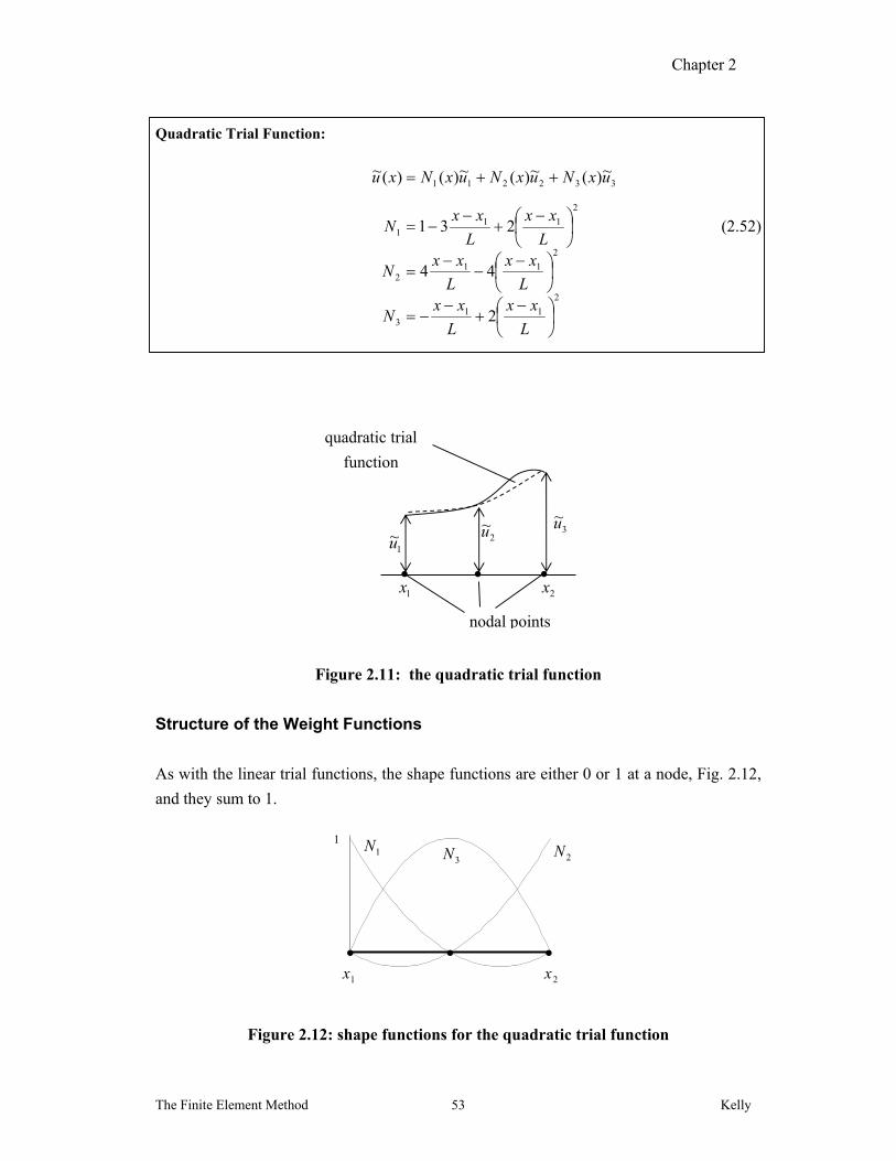
Figure 2.11: the quadratic trial function
Structure of the Weight Functions
As with the linear trial functions, the shape functions are either 0 or 1 at a node, Fig. 2.12,
and they sum to 1.
Figure 2.12: shape functions for the quadratic trial function
1x 2x
quadratic trial
function
3~u
1~u
nodal points
2~u
11N
2N3N
1x 2x
Chapter 2
The Finite Element Method Kelly 54
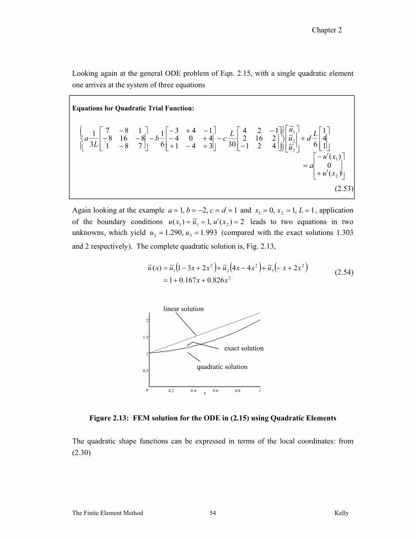
Looking again at the general ODE problem of Eqn. 2.15, with a single quadratic element
one arrives at the system of three equations
Equations for Quadratic Trial Function:
)(0
)(141
6~~~
4212162124
30341404143
6
1
7818168
187
3
1
2
1
3
2
1
xu
xua
Ld
uuuL
cbL
a
(2.53)
Again looking at the example 1,2,1 dcba and 1,1,0 21 Lxx , application
of the boundary conditions 2)(,1~)( 211 xuuxu leads to two equations in two
unknowns, which yield 993.1,290.1 32 uu (compared with the exact solutions 1.303
and 2 respectively). The complete quadratic solution is, Fig. 2.13,
2
23
22
21
826.0167.01
2~44~231~)(~
xx
xxuxxuxxuxu
(2.54)
Figure 2.13: FEM solution for the ODE in (2.15) using Quadratic Elements
The quadratic shape functions can be expressed in terms of the local coordinates: from
(2.30)
0
0.5
1
1.5
2
0.2 0.4 0.6 0.8 1x
linear solution
quadratic solution
exact solution
Chapter 2
The Finite Element Method Kelly 55
Quadratic Shape Functions (Local Coordinates)
12
1,1,1
2
13
221 NNN (2.55)
Note that with a quadratic trial function, one does not need to integrate the higher order
term by parts in order to obtain a solution. However, integration by parts will ensure that
the resulting coefficient matrix is symmetric8, and is done here.
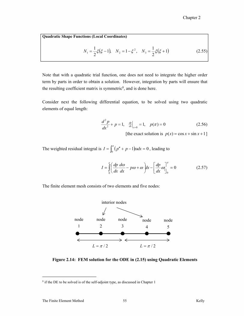
Consider next the following differential equation, to be solved using two quadratic
elements of equal length:
0)(,1,102
2
ppdx
pdxdx
dp (2.56)
[the exact solution is 1sincos)( xxxp ]
The weighted residual integral is 010
dxppI
, leading to
000
dx
dpdxp
dx
d
dx
dpI (2.57)
The finite element mesh consists of two elements and five nodes:
Figure 2.14: FEM solution for the ODE in (2.15) using Quadratic Elements
8 if the DE to be solved is of the self-adjoint type, as discussed in Chapter 1
node
1
node
2
node
3
interior nodes
2/L
node
4
node
5
2/L
Chapter 2
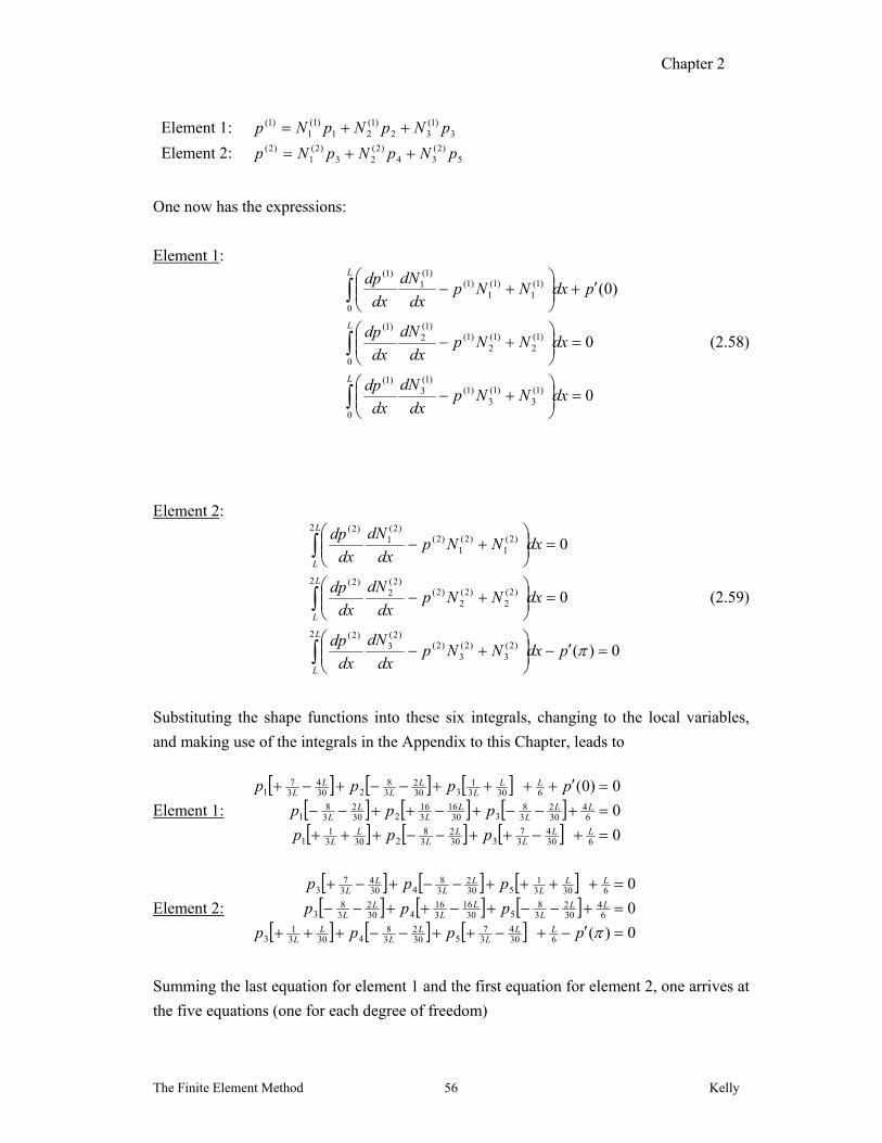
The Finite Element Method Kelly 56
Element 1: 3)1(
32)1(
21)1(
1)1( pNpNpNp
Element 2: 5)2(
34)2(
23)2(
1)2( pNpNpNp
One now has the expressions:
Element 1:
0
0
)0(
0
)1(3
)1(3
)1()1(
3)1(
0
)1(2
)1(2
)1()1(
2)1(
0
)1(1
)1(1
)1()1(
1)1(
dxNNpdx
dN
dx
dp
dxNNpdx
dN
dx
dp
pdxNNpdx
dN
dx
dp
L
L
L
(2.58)
Element 2:
0)(
0
0
2)2(
3)2(
3)2(
)2(3
)2(
2)2(
2)2(
2)2(
)2(2
)2(
2)2(
1)2(
1)2(
)2(1
)2(
pdxNNpdx
dN
dx
dp
dxNNpdx
dN
dx
dp
dxNNpdx
dN
dx
dp
L
L
L
L
L
L
(2.59)
Substituting the shape functions into these six integrals, changing to the local variables,
and making use of the integrals in the Appendix to this Chapter, leads to
Element 1:
0
0
0)0(
6304
37
3302
38
23031
1
64
302
38
33016
316
2302
38
1
63031
3302
38
2304
37
1
LLL
LL
LL
LLL
LL
LL
LLL
LL
LL
ppp
ppp
pppp
Element 2:
0)(
0
0
6304
37
5302
38
43031
3
64
302
38
53016
316
4302
38
3
63031
5302
38
4304
37
3
pppp
ppp
ppp
LLL
LL
LL
LLL
LL
LL
LLL
LL
LL
Summing the last equation for element 1 and the first equation for element 2, one arrives at
the five equations (one for each degree of freedom)
Chapter 2
The Finite Element Method Kelly 57
)(6
4
2
4
)0(6
6
1
4702801000
2801616028000
10280814028010
0028016160280
0010280470
30
1
5
4
3
2
1
222
222
22222
222
222
pL
L
L
L
pL
p
p
p
p
p
LLL
LLL
LLLLL
LLL
LLL
L
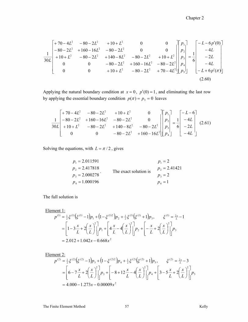
(2.60)
Applying the natural boundary condition at 0x , 1)0( p , and eliminating the last row
by applying the essential boundary condition 0)( 5 pp leaves
L
L
L
L
p
p
p
p
LL
LLLL
LLL
LLL
L
4
2
4
6
6
1
1616028000
280814028010
028016160280
010280470
30
1
4
3
2
1
22
2222
222
222
(2.61)
Solving the equations, with 2/L , gives
000196.1
000278.2
417818.2
011591.2
4
3
2
1
p
p
p
p
. The exact solution is
1
2
41421.2
2
4
3
2
1
p
p
p
p
The full solution is
Element 1:
2
3
2
2
2
1
2
2)1(3
)1()1(21
22)1(
1)1()1(
21)1(
668.0042.1012.2
244231
1,111
xx
pL
x
L
xp
L
x
L
xp
L
x
L
x
pppp Lx
Element 2:
2
5
2
4
2
3
2
2)2(5
)2()2(21
42)2(
3)2()2(
21)2(
00009.0273.1000.4
2534128276
3,111
xx
pL
x
L
xp
L
x
L
xp
L
x
L
x
pppp Lx
Chapter 2
The Finite Element Method Kelly 58
which is very accurate.
2.8 Cubic Hermite Finite Elements
Here the 1C cubic Hermite trial function is examined.
2.8.1 Cubic Hermite Trial Function
The purpose of introducing the cubic Hermite element is to ensure that the first derivatives
of the trial function are continuous at the nodes. To this end, consider four unknowns, the two values of p at the element ends and the two values of p at the element ends. With
four unknowns, one can use the cubic trial function
32)( dxcxbxaxp (2.62)
Using the four equations
22112211 )(,)(,)(,)( pxppxppxppxp (2.63)
to re-write the trial function in terms of the unknown nodal values, one arrives at (after
some lengthy algebra)
Chapter 2
The Finite Element Method Kelly 59
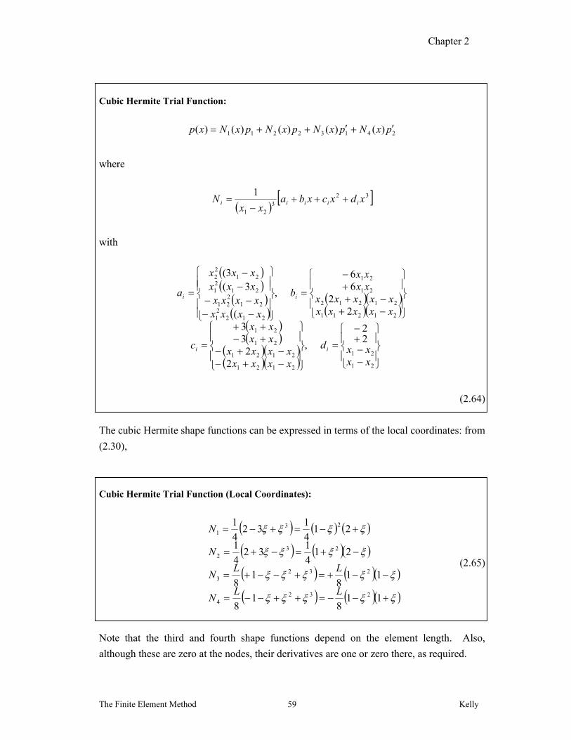
Cubic Hermite Trial Function:
24132211 )()()()()( pxNpxNpxNpxNxp
where
32
321
1xdxcxba
xxN iiiii
with
21
21
2121
2121
21
21
21211
21212
21
21
21221
21221
2121
2122
22
,
22
33
22
66
,
(
3(3(
xxxxd
xxxxxxxx
xxxx
c
xxxxxxxxxx
xxxx
b
xxxxxxxx
xxxxxx
a
ii
ii
(2.64)
The cubic Hermite shape functions can be expressed in terms of the local coordinates: from
(2.30),
Cubic Hermite Trial Function (Local Coordinates):
118
18
118
18
214
132
4
1
214
132
4
1
2324
2323
232
231
LLN
LLN
N
N
(2.65)
Note that the third and fourth shape functions depend on the element length. Also,
although these are zero at the nodes, their derivatives are one or zero there, as required.
Chapter 2
The Finite Element Method Kelly 60
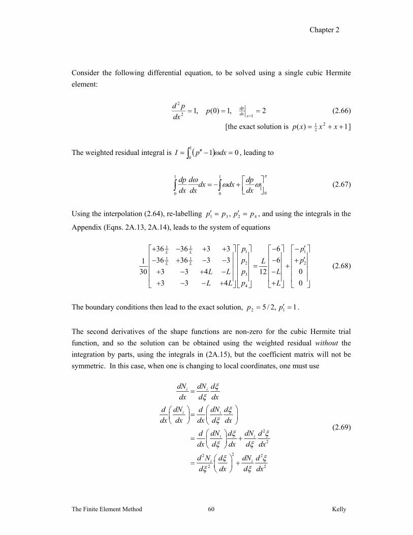
Consider the following differential equation, to be solved using a single cubic Hermite
element:
2,1)0(,112
2
xdx
dppdx
pd (2.66)
[the exact solution is 1)( 221 xxxp ]
The weighted residual integral is 011
0 dxpI , leading to
0
1
0
1
0
dx
dpdxdx
dx
d
dx
dp (2.67)
Using the interpolation (2.64), re-labelling 4231 , pppp , and using the integrals in the
Appendix (Eqns. 2A.13, 2A.14), leads to the system of equations
1 1
1 1
1 12 2
3
4
636 36 3 3
636 36 3 31
03 3 430 12
03 3 4
L L
L L
p p
p pLp LL L
p LL L
(2.68)
The boundary conditions then lead to the exact solution, 1,2/5 12 pp .
The second derivatives of the shape functions are non-zero for the cubic Hermite trial
function, and so the solution can be obtained using the weighted residual without the
integration by parts, using the integrals in (2A.15), but the coefficient matrix will not be
symmetric. In this case, when one is changing to local coordinates, one must use
2
2
22 2
2 2
i i
i i
i i
i i
dN dN d
dx d dx
dN dNd d d
dx dx dx d dx
dN dNd d d
dx d dx d dx
d N dNd d
d dx d dx
(2.69)
Chapter 2
The Finite Element Method Kelly 61
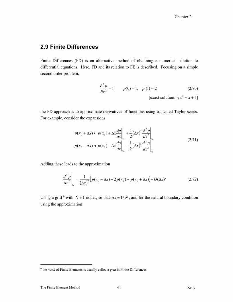
2.9 Finite Differences
Finite Differences (FD) is an alternative method of obtaining a numerical solution to
differential equations. Here, FD and its relation to FE is described. Focusing on a simple
second order problem,
2)1(,1)0(,12
2
ppx
p (2.70)
[exact solution: 1221 xx ]
the FD approach is to approximate derivatives of functions using truncated Taylor series.
For example, consider the expansions
00
00
2
22
00
2
22
00
2
1)()(
2
1)()(
xx
xx
dx
pdx
dx
dpxxpxxp
dx
pdx
dx
dpxxpxxp
(2.71)
Adding these leads to the approximation
2
00022
2
)()()(2)(1
0
xOxxpxpxxpxdx
pd
x
(2.72)
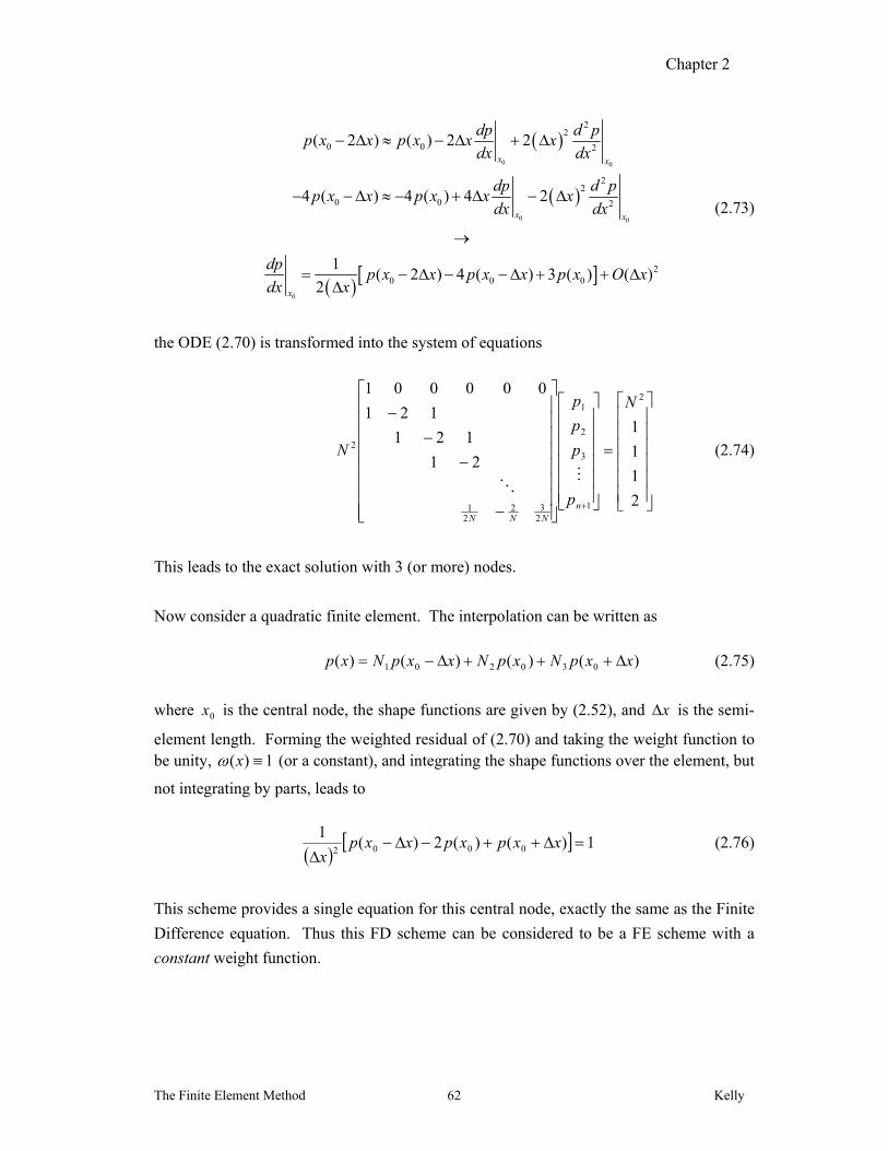
Using a grid 9 with 1N nodes, so that Nx /1 , and for the natural boundary condition
using the approximation
9 the mesh of Finite Elements is usually called a grid in Finite Differences
Chapter 2
The Finite Element Method Kelly 62
0 0
0 0
0
22
0 0 2
22
0 0 2
20 0 0
( 2 ) ( ) 2 2
4 ( ) 4 ( ) 4 2
1( 2 ) 4 ( ) 3 ( ) ( )
2
x x
x x
x
dp d pp x x p x x x
dx dx
dp d pp x x p x x x
dx dx
dpp x x p x x p x O x
dx x
(2.73)
the ODE (2.70) is transformed into the system of equations
2
1
1
1
21
121
121
0000012
1
3
2
1
232
21
2
N
p
p
p
p
N
nNNN
(2.74)
This leads to the exact solution with 3 (or more) nodes.
Now consider a quadratic finite element. The interpolation can be written as
)()()()( 030201 xxpNxpNxxpNxp (2.75)
where 0x is the central node, the shape functions are given by (2.52), and x is the semi-
element length. Forming the weighted residual of (2.70) and taking the weight function to be unity, 1)( x (or a constant), and integrating the shape functions over the element, but
not integrating by parts, leads to
1)()(2)(
10002
xxpxpxxpx
(2.76)
This scheme provides a single equation for this central node, exactly the same as the Finite
Difference equation. Thus this FD scheme can be considered to be a FE scheme with a
constant weight function.
Chapter 2
The Finite Element Method Kelly 63
2.10 Application: Static Elasticity (Structural Mechanics)
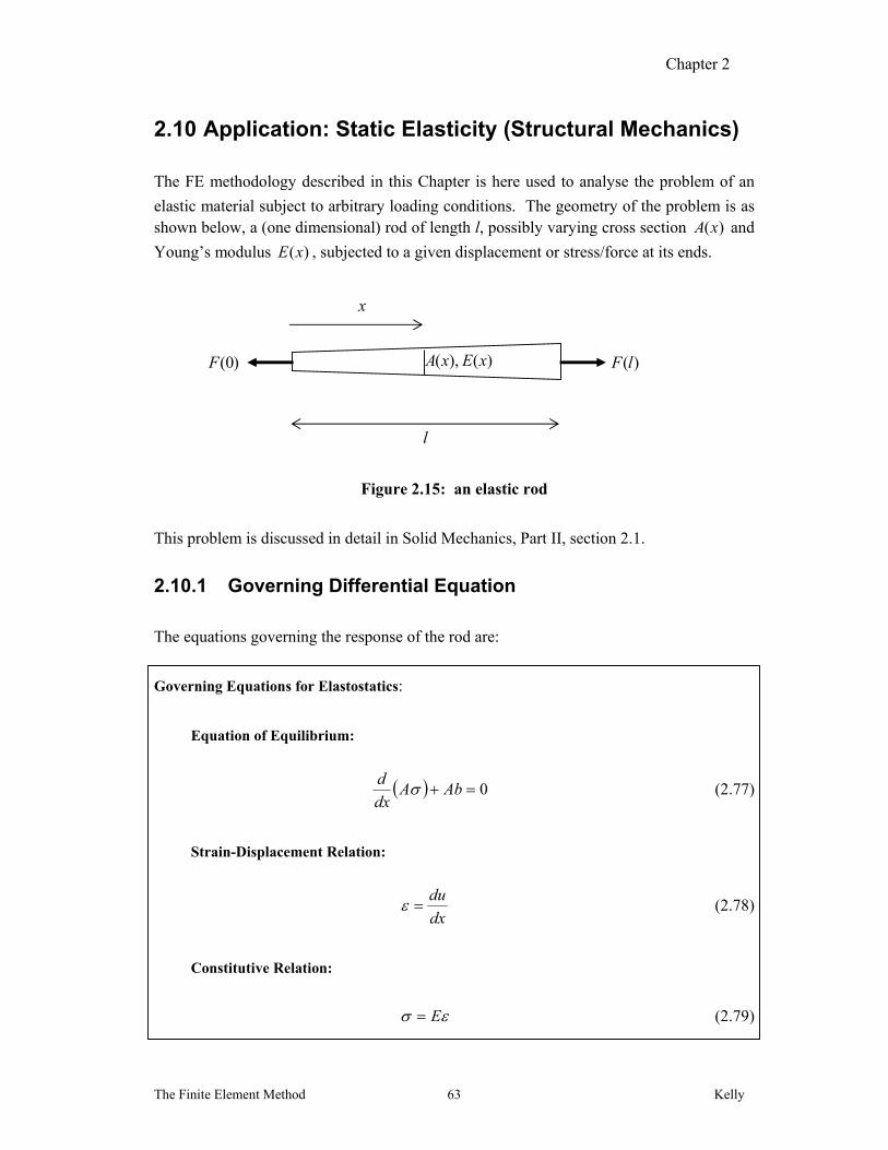
The FE methodology described in this Chapter is here used to analyse the problem of an
elastic material subject to arbitrary loading conditions. The geometry of the problem is as shown below, a (one dimensional) rod of length l, possibly varying cross section )(xA and
Young’s modulus )(xE , subjected to a given displacement or stress/force at its ends.
Figure 2.15: an elastic rod
This problem is discussed in detail in Solid Mechanics, Part II, section 2.1.
2.10.1 Governing Differential Equation
The equations governing the response of the rod are:
Governing Equations for Elastostatics:
Equation of Equilibrium:
0 AbAdx
d (2.77)
Strain-Displacement Relation:
dx
du (2.78)
Constitutive Relation:
E (2.79)
l
x
)(),( xExA)0(F )(lF
Chapter 2
The Finite Element Method Kelly 64
The first two of these are derived in the Appendix to this Chapter, §2.12.2. The third is
Hooke’s experimental law, which is valid for elastic materials undergoing small strains.
In these equations, is the stress, is the small strain (change in length per original
length) and u is the displacement. The constant of proportionality in the linear elastic
constitutive law is E, the Young’s modulus of the material; b is a body force (per unit
volume), for example the force of gravity, and A is the cross-sectional area.
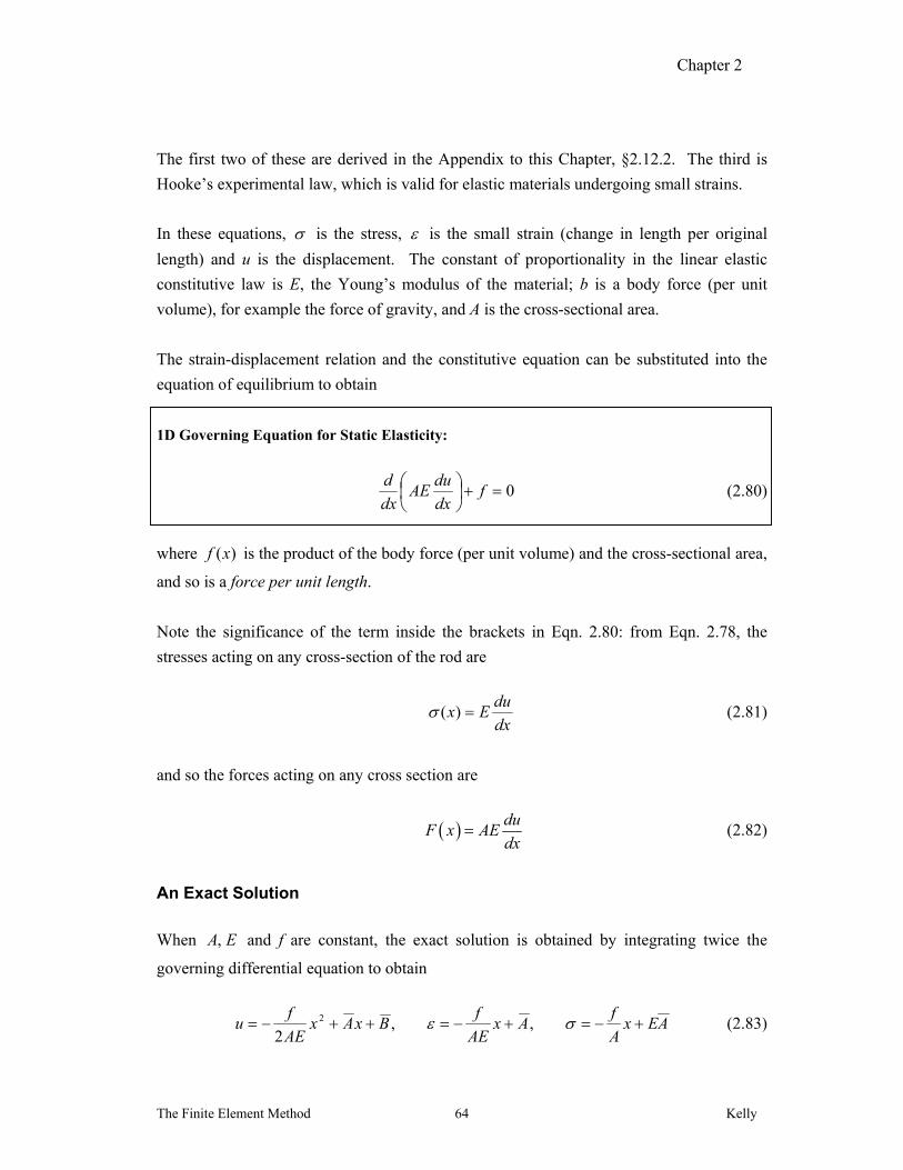
The strain-displacement relation and the constitutive equation can be substituted into the
equation of equilibrium to obtain
1D Governing Equation for Static Elasticity:
0
fdx
duAE
dx
d (2.80)
where )(xf is the product of the body force (per unit volume) and the cross-sectional area,
and so is a force per unit length.
Note the significance of the term inside the brackets in Eqn. 2.80: from Eqn. 2.78, the
stresses acting on any cross-section of the rod are
dx
duEx )( (2.81)
and so the forces acting on any cross section are
duF x AE
dx (2.82)
An Exact Solution
When EA, and f are constant, the exact solution is obtained by integrating twice the
governing differential equation to obtain
AExA
fAx
AE
fBxAx
AE
fu ,,
22 (2.83)
Chapter 2
The Finite Element Method Kelly 65
where A and B are constants to be determined from the boundary conditions.
2.10.2 FEM Formulation
Formally applying the Galerkin method to the one dimensional static elasticity problem
and integrating by parts leads to
lll
dx
duAEdxfdx
dx
d
dx
duAE
000
(2.84)
Trial Function & Boundary Conditions
The trial function for the GFEM is of the form
1
( ) ( )n
i ii
u x x u
(2.85)
where n is the number of nodes in the element, the iu are the unknown nodal values and
the i are the weighting functions. With the shape functions iN as the weights,
substituting into Eqn. 2.84 gives
1 0 0 0
ll lnji
i j ji
dNdN duAE dx u f x N dx AE N
dx dx dx
(2.86)
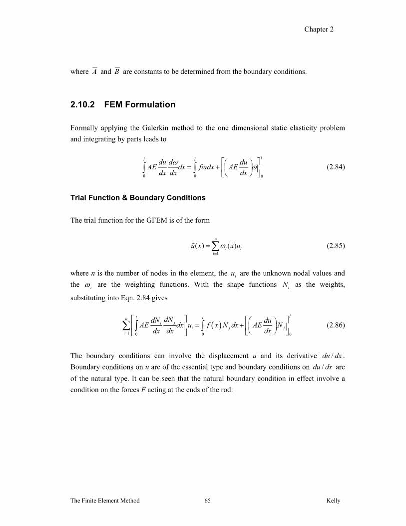
The boundary conditions can involve the displacement u and its derivative dxdu / .
Boundary conditions on u are of the essential type and boundary conditions on dxdu / are
of the natural type. It can be seen that the natural boundary condition in effect involve a
condition on the forces F acting at the ends of the rod:
Chapter 2
The Finite Element Method Kelly 66
Boundary conditions for Static Elasticity:
lllxx
l FAdx
duAEFA
dx
duAEuluuu
,,)(,)0( 000
0 (2.87)
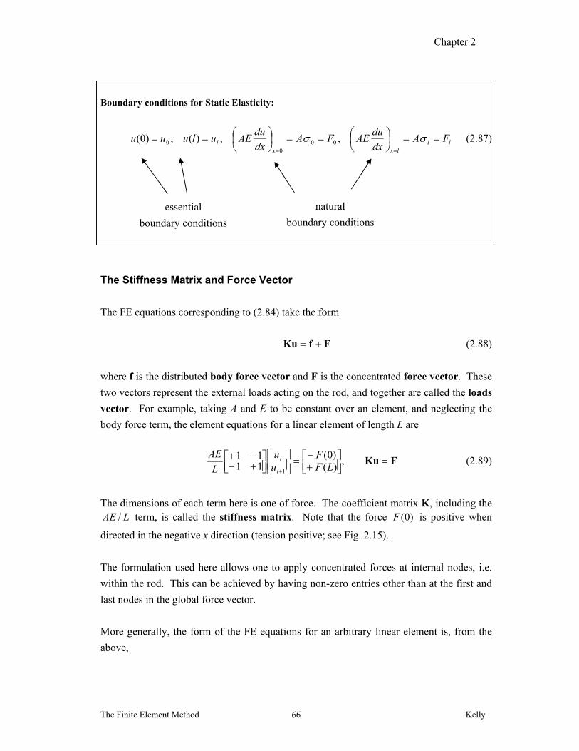
The Stiffness Matrix and Force Vector
The FE equations corresponding to (2.84) take the form
FfKu (2.88)
where f is the distributed body force vector and F is the concentrated force vector. These
two vectors represent the external loads acting on the rod, and together are called the loads
vector. For example, taking A and E to be constant over an element, and neglecting the
body force term, the element equations for a linear element of length L are
FKu
,
)()0(
1111
1 LFF
uu
L
AE
i
i (2.89)
The dimensions of each term here is one of force. The coefficient matrix K, including the LAE / term, is called the stiffness matrix. Note that the force )0(F is positive when
directed in the negative x direction (tension positive; see Fig. 2.15).
The formulation used here allows one to apply concentrated forces at internal nodes, i.e.
within the rod. This can be achieved by having non-zero entries other than at the first and
last nodes in the global force vector.
More generally, the form of the FE equations for an arbitrary linear element is, from the
above,
essential
boundary conditions
natural
boundary conditions
Chapter 2
The Finite Element Method Kelly 67
1 1 1
11 1
1 1 1 21
1 12 1 2 22
i i i
i i i
ii i
ii i
x x x
x x xi i
xx xi i
xx x
dN dN dN dNAE dx AE dx f x N dxu Fdx dx dx dx
u FdN dN dN dN f x N dxAE dx AE dxdx dx dx dx
(2.90)
The stiffness matrix K is singular. This means that if no essential BC is applied (so that a
row can be eliminated), then no solution can be obtained. Physically, an absence of an
essential BC means that there is only an application of forces at the rod-ends (natural BCs),
but no applied displacement. A singular matrix occurs when a structure is not adequately
supported, in this case the rod can undergo an arbitrary rigid body translation – this must
be prevented by at least one essential BC.
The diagonal terms of K must be positive. To see this, suppose that 01 iu . Then,
neglecting the body force term, 11 i iK u F . iF is defined positive in the negative x
direction, and one must have the displacement iu directed the same way as the force (so
0iu if 1 0iu ), and hence 011 K , and similarly for other diagonal terms.
It can also be proved that the elasticity stiffness matrix K is positive definite, i.e.
0T Kxx , for any arbitrary vector x. For example, in the example given above, Eqn. 2.89,
011
11 221
2
121
xxL
AE
x
x
L
AExx (2.91)
Example
Consider a rod with varying cross section )1()( 0 xAxA , constant E and f, and boundary
conditions FlFu )(,0)0( . The exact solution to this problem is seen to be
xFxxlfEA
xu 1ln1ln11
)(0
(2.92)
For a quadratic element, the element equations are, assuming A to be constant,
)(0
)0(
141
67818168
187
33
2
1
LF
FLf
uuu
L
AE (2.93)
Chapter 2
The Finite Element Method Kelly 68
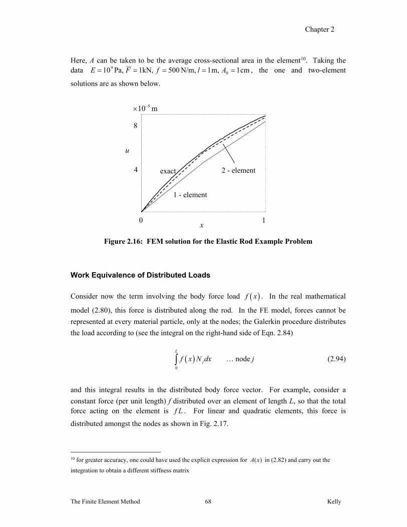
Here, A can be taken to be the average cross-sectional area in the element10. Taking the data cm1,m1N/m,5001kN,Pa,10 0
9 AlfFE , the one and two-element
solutions are as shown below.
Figure 2.16: FEM solution for the Elastic Rod Example Problem
Work Equivalence of Distributed Loads
Consider now the term involving the body force load f x . In the real mathematical
model (2.80), this force is distributed along the rod. In the FE model, forces cannot be
represented at every material particle, only at the nodes; the Galerkin procedure distributes
the load according to (see the integral on the right-hand side of Eqn. 2.84)
0
L
jf x N dx … node j (2.94)
and this integral results in the distributed body force vector. For example, consider a
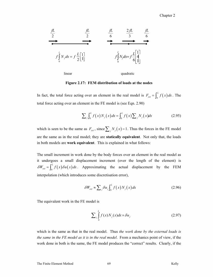
constant force (per unit length) f distributed over an element of length L, so that the total force acting on the element is f L . For linear and quadratic elements, this force is
distributed amongst the nodes as shown in Fig. 2.17.
10 for greater accuracy, one could have used the explicit expression for )(xA in (2.82) and carry out the
integration to obtain a different stiffness matrix
0 1
u
4
8
m10 5
exact
1 - element
2 - element
x
Chapter 2
The Finite Element Method Kelly 69
Figure 2.17: FEM distribution of loads at the nodes
In fact, the total force acting over an element in the real model is 0
L
extF f x dx . The
total force acting over an element in the FE model is (see Eqn. 2.90)
0 0
L L
j jj jf x N x dx f x N x dx (2.95)
which is seen to be the same as extF , since 1jj
N x . Thus the forces in the FE model
are the same as in the real model; they are statically equivalent. Not only that, the loads
in both models are work equivalent. This is explained in what follows:
The small increment in work done by the body forces over an element in the real model as
it undergoes a small displacement increment (over the length of the element) is
0
L
extW f x u x dx . Approximating the actual displacement by the FEM
interpolation (which introduces some discretisation error),
0
L
ext j jjW u f x N x dx (2.96)
The equivalent work in the FE model is
0
( ) ( )L
j jjf x N x dx u (2.97)
which is the same as that in the real model. Thus the work done by the external loads is
the same in the FE model as it is in the real model. From a mechanics point of view, if the
work done in both is the same, the FE model produces the “correct” results. Clearly, if the
quadratic linear
2
fL
2
fL
6
fL
3
2 fL
6
fL
11
20
LfdxNf
L
j
141
60
LfdxNf
L
j
Chapter 2
The Finite Element Method Kelly 70
forces were distributed in some other way, the work done in the FE model would not be the
true work done, and the FE model would give spurious results.
Internal Forces and Internal Work
Internal forces arise within the elastic material to equilibrate the externally applied forces.
Whereas the external forces are due to some external agency, for example gravity, or an
applied load, the internal forces are a result of the stresses which arise within the deformed
material. As the external forces perform work, so do the internal forces: the internal work
is a result of the internal forces moving through some displacement.
As with the external forces, the internal forces are distributed amongst the nodes in the FE
model. Since the FE equations are FfKu , and the right-hand side represents the
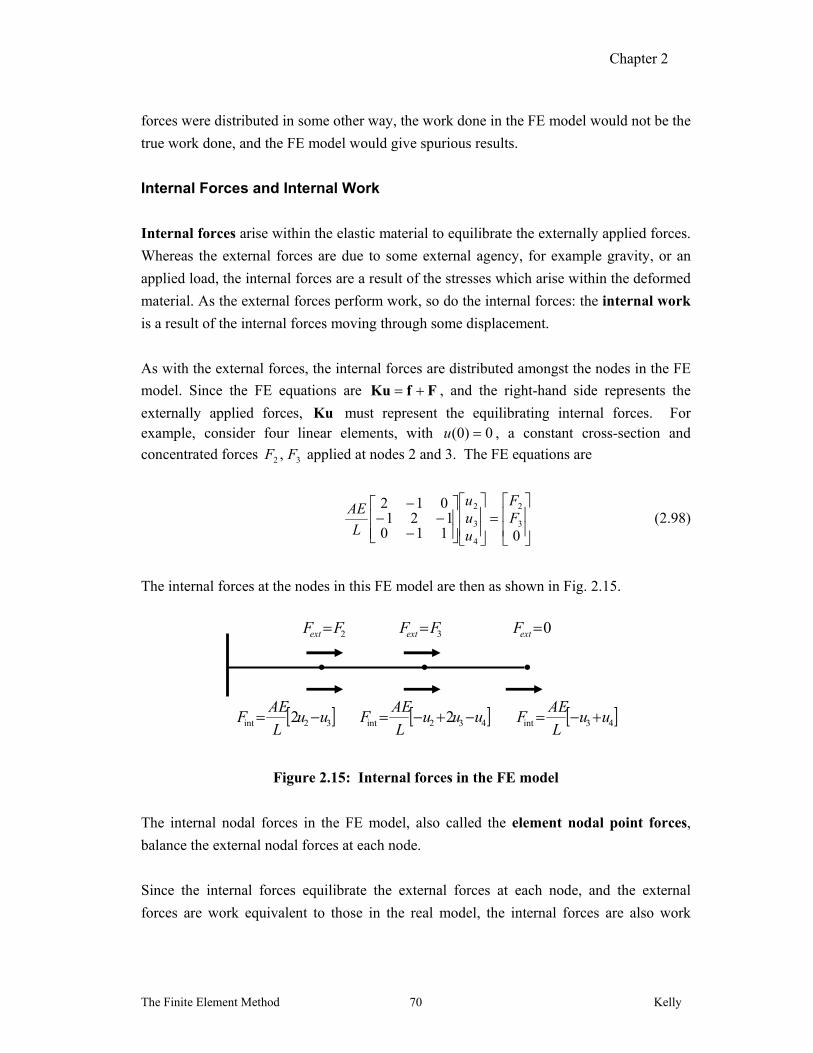
externally applied forces, Ku must represent the equilibrating internal forces. For example, consider four linear elements, with 0)0( u , a constant cross-section and
concentrated forces 32 , FF applied at nodes 2 and 3. The FE equations are
0110121
0123
2
4
3
2
FF
uuu
L
AE (2.98)
The internal forces at the nodes in this FE model are then as shown in Fig. 2.15.
Figure 2.15: Internal forces in the FE model
The internal nodal forces in the FE model, also called the element nodal point forces,
balance the external nodal forces at each node.
Since the internal forces equilibrate the external forces at each node, and the external
forces are work equivalent to those in the real model, the internal forces are also work
32int 2 uuL
AEF 432int 2 uuu
L
AEF 43int uu
L
AEF
2FFext 3FFext 0extF
Chapter 2
The Finite Element Method Kelly 71
equivalent to those in the real model. This point is better illustrated in the context of the
potential energy of the deforming system, discussed in the following section.
2.10.3 Variational Formulation
The variational approach was introduced in Chapter 1, section 1.3. (See also the detailed
discussion of the variational approach in sections 8.5 and 8.6 of Solid Mechanics, Part I.)
Following that procedure, beginning again, the governing equation of static elasticity, Eqn.
2.80, is
0
fdx
duAE
dx
d (2.99)
Multiplying the equation across by a small displacement u x ,
0d du
AE u f udx dx
(2.100)
Recall that each term in Eqn. 2.99 has units of force (per unit length), and so the terms in
Eqn 2.100 have units of work (per unit length). Integrating over the element gives the total
work due to the change in displacement:
0
0l l
o
d duAE u dx f u dx
dx dx
(2.101)
Integrating by parts and using the results from the Calculus of Variations derived and given
in section 1.3, this can now be re-expressed as
2
00
10
2
ll l
o
du duAE dx AE u f u dx
dx dx (2.102)
It will be recognised that the term 2120
/l
AE du dx dx is the strain energy in the bar (see,
for example, Eqn. 8.2.3 in Solid Mechanics, Part I, with the force given by Eqn. 2.82).
Thus Eqn. 2.102 can be expressed as
Chapter 2
The Finite Element Method Kelly 72
0 (2.103)
where is the potential (strain) energy. Taking the potential energy to be a function of the
displacement, Eqn. 2.103 can be expressed as
0d u
udu
(2.104)
which is an expression of the principle of minimum potential energy: the solution to the
structural mechanics problem is that which causes the potential energy to be stationary,
/ 0d du .
Using now the displacement interpolation i iu N u ,
2
00
1
2
ll li
i i i i i
o
dN duAE u dx AE N u f N u dx
dx dx
(2.105)
Introducing row vectors for the shape functions:
1 2 1 2, / /N N dN dx dN dx N B (2.106)
and the column vector of unknown nodal displacements
1
2
u
u
u (2.107)
Eqn. 2.105 can be expressed as (for linear elements, but this can be generalised in the same
way for other elements):
00
1
2
ll lTT
o
duAE dx AE f dx
dx
u B B u N u N u (2.108)
The stationary value of the energy can now be obtained by differentiating this expression
with respect to the vector u. For the purposes of differentiation with respect to
matrices/vectors, note the following rules:
Chapter 2
The Finite Element Method Kelly 73
Consider the scalar function of a vector u: 1 1 2 2N u N u u N u . Differentiation of
a scalar with respect to a vector produces a vector:
1 1
2 2
/
/Tu N
u N
uN
u (2.109)
Consider next the scalar function 2
1 1 2 2
TTB u B u u u B B u . Differentiation
gives:
1 1 1 2 21
2 1 1 2 22
2/2
2/TB B u B uu
B B u B uu
uB B u
u (2.110)
Thus the stationary point of Eqn. 2.108 is given by
00
ll lT
o
d duAE dx AE f dx
d dx
T Tu
B B u N Nu
(2.111)
Setting this to zero then gives
00
ll lT
o
duAE dx AE f dx
dx
T T
B B u N N (2.112)
which is exactly the same as Eqn. 2.90 derived earlier directly from the governing
differential equation.
Thus the FE equations can be derived either directly from the governing differential
equation or through the variational approach. When using the variational approach, the
potential (strain) energy of the system enters directly, and in that sense one says that the
finite element model is energy or work equivalent to the real model.
2.11 Problems
1. Solve the following problem using two linear elements of equal length:
3)2(,1)0(,62
2
uuxdx
ud [exact sln. 13)( 3 xxxu ]
Chapter 2
The Finite Element Method Kelly 74
To deal with the non-homogeneous term, you might proceed in one of two ways: (i) use the linear interpolation 1 1 26 6 i ix x N x N - which is in this case of course
exact since the function x6 is linear
(ii) after converting to local coordinates, evaluate the resulting integrals dNx j6
exactly using the relation (2.A6)
13
13
3
11
1 A
AdANi
Evaluate also the FE solution for p . Sketch the exact, FE and smoothed solutions
for p .
2. Re-solve the ODE of Problem 1, only now with a natural boundary condition at 2x : 6/ 2 xdxdp [the exact solution is 16)( 3 xxxp ]
3. Solve the problem 0)3(,1)0(,0 ppxp with two linear elements of
lengths 1 and 2 respectively. Work through the problem in detail, using local coordinates. Derive an expression for p in each element.
[answer: element 1 - 313p , element 2 - 3
7p ]
4. What is a 1C element?
5. What is adaptive meshing? How might an adaptive meshing procedure be
implemented with 0C elements (briefly explain)?
6. What are the sources of error in the FEM (explain any terminology you might use)?
7. Derive Eqns. 2.52, the shape functions for the quadratic element. 8. Consider the equation )(xfp . Write down, as quick as you can, the global
stiffness matrix for (consult the notes)
a) a mesh of 5 linear 1-d elements, each of length 2. b) a mesh of 3 quadratic 1-d elements, each of length 3
1 .
9. For the (Galerkin) FEM, in a 2nd-order problem, why does one integrate by parts to
reduce the order of the highest derivative to 1? Is this always necessary?
10. Note that, in the coefficient matrices encountered in this Chapter, e.g. Eqns. 2.24,
2.27, 2.53, 2.60, the entries of any row or column sum to zero. Using the properties
of the shape functions, explain why this is so, and why it is not so for the matrix
(2.68) of the cubic Hermite element.
Chapter 2
The Finite Element Method Kelly 75
2.12 Appendix to Chapter 2
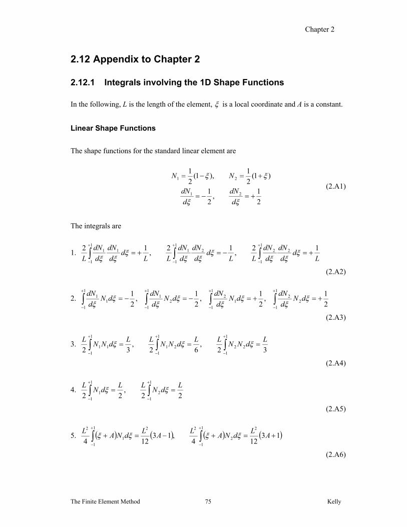
2.12.1 Integrals involving the 1D Shape Functions In the following, L is the length of the element, is a local coordinate and A is a constant.
Linear Shape Functions
The shape functions for the standard linear element are
2
1,
2
1
)1(2
1),1(
2
1
21
21
d
dN
d
dN
NN
(2.A1)
The integrals are
1. L
dd
dN
d
dN
LLd
d
dN
d
dN
LLd
d
dN
d
dN
L
12,
12,
12 1
1
221
1
211
1
11
(2.A2)
2. 2
1,
2
1,
2
1,
2
1 1
1
22
1
1
12
1
1
21
1
1
11
dNd
dNdN
d
dNdN
d
dNdN
d
dN
(2.A3)
3. 32
,62
,32
1
1
22
1
1
21
1
1
11
LdNN
LLdNN
LLdNN
L
(2.A4)
4. 22
,22
1
1
2
1
1
1
LdN
LLdN
L
(2.A5)
5. 13124
,13124
21
1
2
221
1
1
2
AL
dNAL
AL
dNAL
(2.A6)
Chapter 2
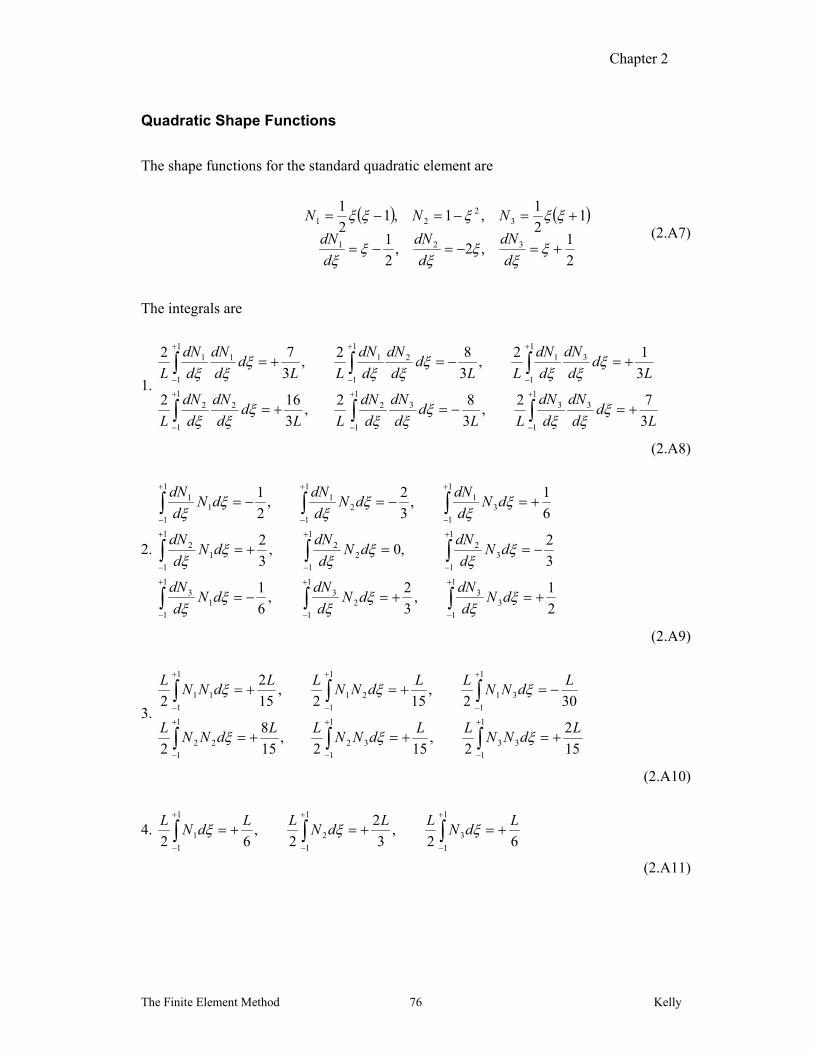
The Finite Element Method Kelly 76
Quadratic Shape Functions
The shape functions for the standard quadratic element are
2
1,2,
2
1
12
1,1,1
2
1
321
32
21
d
dN
d
dN
d
dN
NNN (2.A7)
The integrals are
1.
Ld
d
dN
d
dN
LLd
d
dN
d
dN
LLd
d
dN
d
dN
L
Ld
d
dN
d
dN
LLd
d
dN
d
dN
LLd
d
dN
d
dN
L
3
72,
3
82,
3
162
3
12,
3
82,
3
72
1
1
331
1
321
1
22
1
1
311
1
211
1
11
(2.A8)
2.
2
1,
3
2,
6
1
3
2,0,
3
2
6
1,
3
2,
2
1
1
1
33
1
1
23
1
1
13
1
1
32
1
1
22
1
1
12
1
1
31
1
1
21
1
1
11
dNd
dNdN
d
dNdN
d
dN
dNd
dNdN
d
dNdN
d
dN
dNd
dNdN
d
dNdN
d
dN
(2.A9)
3.
15
2
2,
152,
15
8
2
302,
152,
15
2
21
1
33
1
1
32
1
1
22
1
1
31
1
1
21
1
1
11
LdNN
LLdNN
LLdNN
L
LdNN
LLdNN
LLdNN
L
(2.A10)
4. 62
,3
2
2,
62
1
1
3
1
1
2
1
1
1
LdN
LLdN
LLdN
L
(2.A11)
Chapter 2
The Finite Element Method Kelly 77
5.
)1(124
34),1(
12421
1
3
2
21
1
2
221
1
1
2
AL
dNAL
ALdNA
LA
LdNA
L
(2.A12)
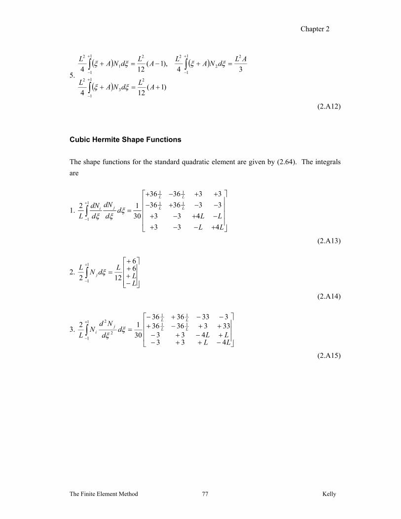
Cubic Hermite Shape Functions
The shape functions for the standard quadratic element are given by (2.64). The integrals
are
1.
1 1
1 1 1
1
36 36 3 3
36 36 3 32 1
3 3 430
3 3 4
L L
j L LidNdN
dL LL d d
L L
(2.A13)
2.
LL
LdN
Lj
66
122
1
1
(2.A14)
3.
LL
LLd
d
NdN
LLL
LL
ji
433433
33336363333636
30
12 11
11
1
12
2
(2.A15)

Chapter 2
The Finite Element Method Kelly 78
2.12.2 Derivation of the Governing Equations for Elasticity
The following are discussed in more detail in Solid Mechanics, Part II, Sections 1.1, 1.2.
Force Balance
Consider a one-dimensional differential element of length x . The element has varying cross secton, with )()()( xOxAxxA . Let a body force (per unit volume) b, e.g.
the force of gravity, act on the element, again, with )()()( xOxbxxb . Denote the
acceleration and density of the element be a and . Stresses act on the element.
The surface forces acting are
xxxAA
. The force due to b is 2)()()( xOxxbxA .
Applying Newton’s second law,
)(
2/)()()( 2
xOaAAbx
AAAAxaxOxxbxAAA
xxx
xxxxxx
(2A.16)
so that, by the definition of the derivative, in the limit as 0x , one has the equation of
motion
aAAbAdx
d (2A.17)
If the material is static, or if the accelerations are so low that they can be neglected, this
equation reduces to the equation of equilibrium:
0 AbAdx
d (2A.18)
)(xA
x
)(x
)( xx
x xx
ab,
)( xxA
Chapter 2
The Finite Element Method Kelly 79
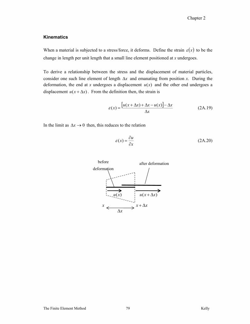
Kinematics
When a material is subjected to a stress/force, it deforms. Define the strain x to be the
change in length per unit length that a small line element positioned at x undergoes.
To derive a relationship between the stress and the displacement of material particles,
consider one such line element of length x and emanating from position x. During the deformation, the end at x undergoes a displacement )(xu and the other end undergoes a
displacement )( xxu . From the definition then, the strain is
x
xxuxxxux
)()(
)( (2A.19)
In the limit as 0x then, this reduces to the relation
x
ux
)( (2A.20)
xx xx
before
deformation after deformation
)(xu )( xxu

Chapter 2
The Finite Element Method Kelly 80