2 STN 11-3 October 2008: New Directions in …such as COCOMO 2.0 in 2000), ... New Directions in Software Estimation. ... implement new features desired for SoS-level capabilities,

STN 11-3 October 2008: New Directions in Software Estimation2

TEch ViEwS by Dan Ferens, DAcS Analyst, iTT corporation

Software estimation appears to be rather uncomplicated. A general equation for estimating software effort is simply:

Effort = f (Size, Productivity)

Where effort is in person-months (or similar), size is in lines of code, function points, or other size measure, and productivity is in size units per unit of time, such as function points per person-month (or, sometimes, time required per size unit, like person-hours per function point). Some early (1970s) models estimated effort using an equation such as

Effort = A x (Size)B

Where A and B are constants, often obtained from historical data. (Note that if B not equal to 1, productivity varies with program size.)

Software schedule has often been computed as a function of effort using an equation such as:

Schedule = C x (Effort)D

Where schedule is in time units such as months, C and D are constants that, like A and B, are often obtained from historical data, and effort is computed from the equation above.

In reality, however, software estimation is quite complex. In fact, Dr. Barry Boehm said that basic models for effort are only accurate to “within a factor of two, 60% of the time [Boehm 81, p. 114]. Productivity is quite difficult to assess; the averages used in models like those above have considerable variation. Factors such as operating environment, personnel capabilities, use of modern practices, hardware constraints, time and person-power limitations, development method, system integration requirements, and security requirements will greatly affect productivity for any given project or program. Schedule can be even more difficult to assess since not only effort must be known, but also other factors which cause variation in the C and D constants for specific programs.

Size is often difficult to estimate, especially early in a program. Lines of code vary by language and by counting practices. Function points, although well-researched, are also sometimes hard to count or estimate, and have not been shown to be appropriate in some situations. Other measures, such as object points and use case points, are also not applicable in some situations and are not as well researched as lines of code and function points.

One other limitation of most basic effort equations is that

they usually address only software development costs. Software maintenance (or support) costs usually exceed software development costs, but some models have not addressed them at all, or only in a cursory manner.

During the late 1970s and during the 1980s, some sophisticated software estimating models were developed such as Dr. Boehm’s Constructive Cost Model (COCOMO), PRICE-S (now True S), SLIM, SEER-SEM, and SPQR/20 (now Knowledge Plan). During the mid 1980s, some sophisticated software size estimating techniques, sometimes included in cost models, came into being. Function points became a measure of size that could be used in addition to (or instead of ) lines of code. Most cost models now included some maintenance estimation capabilities.

Since the late 1980s, the existing models have been improved (such as COCOMO 2.0 in 2000), and new ones have arisen. Models have also been adapted for newer languages, such as Java, and newer development methods such as object-oriented development. Additional size measures such as object points and use case points have been advanced. However, the status of software estimating is not utopian, and there is still room for improvement and for new ideas. For example, an award-winning study by Ferens and Christensen [Ferens 98], using the results of ten Master’s Thesis efforts at the Air Force Institute of Technology, showed that none of the popular cost models were shown to be accurate for two department of defense (DoD) databases. This may have reflected problems with the databases instead of the models, but the end result was that development cost and schedule estimation could not be shown to be accurate. A later study by Brummert and Mischler [Brummert, 1998] showed the problems were even worse for software support, or maintenance estimating. The models varied widely on their estimates, what constitutes support, and how people were allocated during the support period. Size estimating models and methods have been shown accurate, but only for selected types of software applications.

This issue of the Software Tech News, “New Directions in Software Estimation”, describes the migration/evolution that is occurring in software estimating in response to the continuing and emerging challenges of developing and maintaining complex software systems. The first article by Jo Ann Lane and Barry Boehm addresses the emerging interest area of estimating Software-Intensive System of Systems (SISOS) The next article by Don Scott Lucero and Christopher Miller addresses challenges associated with software estimating in the U.S. Department of Defense. The next article by Arlene Minkiewicz addresses the issues associated with software size estimation with suggestions for using sizing methods. Dan Galorath’s

Data & Analysis Center for Software (DACS) 3

article addresses current issues in software maintenance and how we may resolve them. Finally, Capers Jones addresses risk in software estimates, an area that is of great importance but not usually addressed adequately in software estimates.

While the articles in this issue do not constitute a panacea for the challenges associated with software estimating, they will provide the reader with new insights and new ideas in this area. DACS welcomes your comments on this issue or anything related to software engineering and management.

About the AuthorDan Ferens works for ITT AES as an analyst for the DACS

and as an instructor for a 12-part series in software affordability which has been taught mainly to Air Force Research Laboratory (AFRL) scientists, engineers, and managers in Rome, NY. Dan retired from AFRL in early 2007 after more than 35 years of service to the Air Force as a military and civilian employee. Dan has been involved in software estimating since he became a civilian in 1978, both as an AFRL analyst and program manager, and as a Professor at Air Force Institute of Technology where he taught classes on software estimation and other software engineering and management topics for 13 years. He is currently an Adjunct Instructor at SUNY Institute of Technology in Utica, New York where he teaches a class in information technology project management. He is a life

member of the International Society of Parametric Analysts (ISPA), where, in 1999, he received the prestigious Freiman award for lifetime achievements in parametric estimating. Mr. Ferens has a Masters degree in Electrical Engineering from Rensselaer Polytechnic Institute, and a Masters Degree in Business Administration from the University of Northern Colorado. He and his wife, Marcie, currently reside in Fulton, New York.

Author Contact InformationDan Ferens: [email protected]

References:[Boehm 1981] Boehm, Barry W., Software Engineering Economics,

Prentice-Hall, Englewood Cliffs, NJ, 1981.[Ferens 1998] Ferens, Daniel V. and David S Christensen,

“Calibrating Software Cost Models to Department of Defense Databases – A review of Ten Studies”, ISPA Journal of Parametrics, Volume XVIII, Number 2, November, 1998, pp. 55-74.

[Brummert 1998] Brummert, Kevin L., and Philip Mischler, Jr., “Software Support Cost Estimating Models: A Comparative Study of Model Content and Parameter Sensitivity” (AFIT Master’s Thesis), Air Force Institute of Technology, Dayton, OH, September, 1998.

Modern Tools to Support DoD Software Intensive System of Systems Cost EstimationWhen organizations started using sos concepts to evolve and expand the capabilities of their existing systems, they found that their cost estimation tools covered part of the sos development activities, but not all of them.by Jo Ann Lane and Barry Boehm, University of Southern california, center for Systems and Software Engineering

This article summarizes key information in a DACS State of the Art Report published in 2007, also authored by Boehm and Lane, titled “Modern Tools

to Support DoD Software Intensive System of Systems Cost Estimation, available free of charge from the DACS web site.

PurposeAs system development approaches and technologies used

to develop systems evolve, techniques and tools used to plan

and estimate these system development activities likewise need to evolve. This article provides guidance to those attempting to estimate effort needed to develop a System of Systems (SoS). Case studies of previous Software-Intensive SoS (SISOS) projects have found that even very well-planned SISOS projects can encounter unanticipated sources of cost growth [Krygiel, 1999]. The intent is that managers and estimators find this article’s guidance useful when generating estimates to develop or extend SoSs. They should use the guidance and conceptual parameters

TEch ViEwS (cONT.)


presented in this report to reason about their SoS and to make sure that their estimates account for all critical cost factors that pertain to their SoS.

This guidance includes an overview of typical SoS development activities, existing parametric modeling tools that can be applied to SoS estimation activities, as well as additional size drivers and cost factors to be considered when preparing estimates. In particular, this article describes:

• TheuniquechallengesofSISOScostestimation• Howcurrenttoolsarechangingtosupportthese

challenges• On-goingeffortstofurtherunderstandSISOS

development processes and the factors that impact the effort to perform thee processes• CurrenttechniquesandtoolstosupportSISOScost

estimation needs.

This report uses the Constructive Cost Model (COCOMO) family of estimation models as its reference framework, but also incorporates activities underway by other cost model providers.

A review of recent publications [Lane and Valerdi, 2007] shows that the term “system-of-systems” means many things to many different people and organizations. Many seem to be converging on the definition provided in [Maier, 1998]: “an evolutionary net-centric architecture that allows geographically distributed component systems to exchange information and perform tasks within the framework that they are not capable of performing on their own outside of the framework”. The nature of these tasks often cannot be specified in advance but emerges with use. This is often referred to as “emergent behavior”. In addition, the component systems are typically independently managed, have their own purpose, and can operate either on their own or within the SoS.

With the SoS development approach, system development processes are evolving and are being referred to as System of Systems Engineering (SoSE) [SoSECE, 2006; USAF, 2005]. SoSE is that set of engineering activities performed to define the desired SoS-level capabilities, develop the SoS-level architecture, identify sources to either supply or develop the required SoS component systems, then integrate and test these high level components within the SoS architecture framework, with the result being a deployable SoS.

The rest of this report focuses on the estimation of costs associated with the implementation of SoS capabilities using an SoSE team to guide and coordinate SoSE activities. For a detailed description of SoSE activities, see [DoD, 2008].

Inadequacy of traditional cost models in estimating system of systems costs

When organizations started using SoS concepts to evolve and expand the capabilities of their existing systems, they found that their cost estimation tools covered part of the SoS development activities, but not all of them. If an organization decides to acquire or develop a new system to integrate into the SoS (or to facilitate the integration of existing systems into an SoS), then existing systems engineering, software development, and/or Commercial Off-the-Shelf (COTS) integration cost models can be used to estimate the effort associated with the acquisition/development of the system component. An example of this might be a new “translator” component that converts data between different formats so that no modifications are needed for legacy components. Likewise, if changes must be made to existing (legacy) systems in order to enable SoS connectivity or implement new features desired for SoS-level capabilities, the existing cost models can be used to estimate the effort associated with these system-level changes.

What is not covered by existing cost models is the effort associated with the development of the SoS concepts and architecture, the analysis required to identify the desired SoS component systems, and the integration and test of those component systems in the SoS environment. Figure 1 shows the home-grounds of various cost models, as well as highlights the fact that SoSE activities are currently not specifically addressed by existing cost models. Further, the sizing inputs used by the existing models (e.g., number of requirements, function points, lines of application or COTS glue code) are not well-matched to SoSE sources of effort or sources of information

In addition, [Wilson, 2007] provides a comprehensive analysis of several parametric tools either currently being used or under development to support the estimation of SoS development effort. Many of the tools that Wilson analyzed are adaptations of the software and systems engineering tools shown in Figure 1. His conclusion at this point in time is that SoSs are poorly understood and that the tools and thought processes needed to address the development of these systems

MODErN TOOLS TO SUppOrT DOD SOFTwArE iNTENSiVE SySTEM OF SySTEMS cOST ESTiMATiON (cONT.)

Figure 1: Suite of Available Cost Models to Support SISOS Effort Estimation

System of Systems Engineering

Software EngineeringCOCOMO II [Boehm et al, •2005]CostXpert [CostXpert Group, •2003]CoStar [SOFTSTAR, 2006]•Price-S [Price, 2006]•SEE-SEM [Galorath, 2001]•SLIM [QSM, 206]•

Systems EngineeringCOSYSMO [Valerdi, 2005]•

COTS IntegrationCOCOTS [Abts, 2004]•SEER-SEM [Galorath, 2001]•

Hardware EngineeringPrice-H [PRICE, 2006]•SEER-H [Galorath, 2001]•


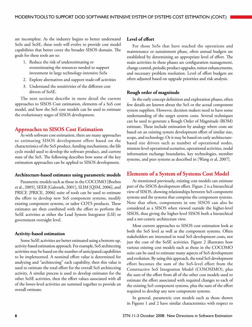
are incomplete. As the industry begins to better understand SoSs and SoSE, these tools will evolve to provide cost model capabilities that better cover the broader SISOS domain. The goals for these tools are to:

1. Reduce the risk of underestimating or overestimating the resources needed to support investment in large technology-intensive SoSs

2. Explore alternatives and support trade-off activities3. Understand the sensitivities of the different cost

drivers of SoSE.The next sections describe in more detail the current

approaches to SISOS Cost estimation, elements of a SoS cost model, and how the SoS cost models can be used to estimate the evolutionary stages of SISOS development.

Approaches to SISOS Cost EstimationAs with software cost estimation, there are many approaches

to estimating SISOS development effort based on the characteristics of the SoS product, funding mechanisms, the life cycle model used to develop the software product, and current state of the SoS. The following describes how some of the key estimation approaches can be applied to SISOS development.

Architecture-based estimates using parametric modelsParametric models such as those in the COCOMO [Boehm

et al., 2005], SEER [Galorath, 2001], SLIM [QSM, 2006], and PRICE [PRICE, 2006] suite of tools can be used to estimate the effort to develop new SoS component systems, modify existing component systems, or tailor COTS products. These estimates are then combined with the effort to perform the SoSE activities at either the Lead System Integrator (LSI) or government oversight level.

Activity-based estimationSome SoSE activities are better estimated using a bottom-up,

activity-based estimation approach. For example, SoS architecting activities may be based on the number of anticipated capabilities to be implemented. A nominal effort value is determined for analyzing and “architecting” each capability, then this value is used to estimate the total effort for the overall SoS architecting activity. A similar process is used to develop estimates for the other SoSE activities, then the effort values associated with all of the lower-level activities are summed together to provide an overall estimate.

Level of effortFor those SoSs that have reached the operations and

maintenance or sustainment phase, often annual budgets are established by determining an appropriate level of effort. The main activities in these phases are configuration management, change control, periodic product upgrades, minor enhancements, and necessary problem resolution. Level of effort budgets are often adjusted based on upgrade priorities and risk analysis.

Rough order of magnitudeIn the early concept definition and exploration phases, often

few details are known about the SoS or the actual component system suppliers. However, decision makers need to have some understanding of the target system costs. Several techniques can be used to generate a Rough Order of Magnitude (ROM) estimate. These include estimation by analogy where costs are based on an existing system development effort of similar size, scope, and technology. Or it may be based on early architecture-based size drivers such as number of operational nodes, mission-level operational scenarios, operational activities, nodal information exchange boundaries, key technologies, member systems, and peer systems as described in [Wang et al, 2007].

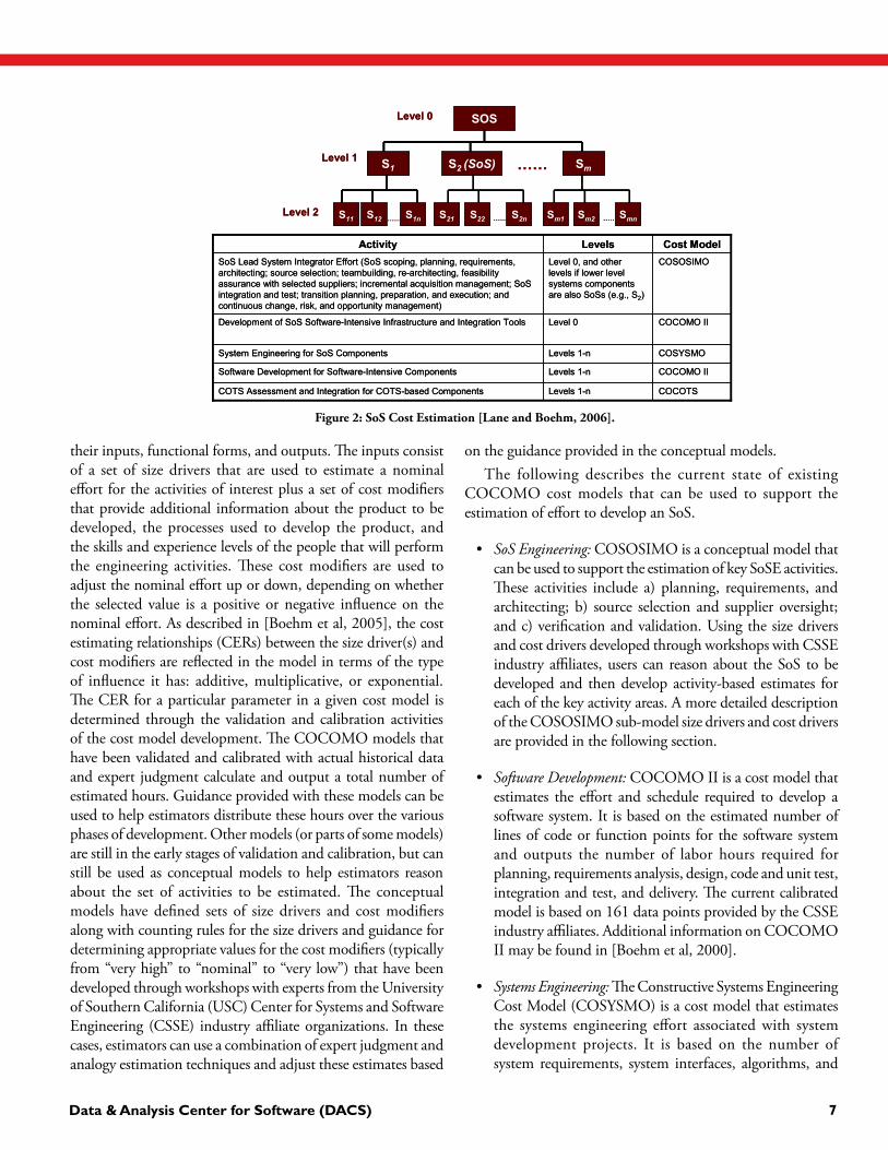
Elements of a System of Systems Cost ModelAs mentioned previously, existing cost models can estimate

part of the SISOS development effort. Figure 2 is a hierarchical view of SISOS, showing relationships between SoS component systems and the systems that comprise the component systems. Note that often, components in one SISOS can also be considered as a SISOS when viewed outside the higher-level SISOS, thus giving the higher-level SISOS both a hierarchical and a net-centric architecture view.

Most current approaches to SISOS cost estimation look at both the SoS level as well as the component systems. Often stakeholders are interested in total SoS development costs, not just the cost of the SoSE activities. Figure 2 illustrates how various existing cost models such as those in the COCOMO suite can be used to estimate many aspects of SoS development and evolution. By using this approach, the total SoS development effort becomes the sum of the SoS-level effort from the Constructive SoS Integration Model (COSOSIMO), plus the sum of the effort from all of the other cost models used to estimate the effort associated with required changes to each of the existing SoS component systems, plus the sum of the effort required to develop any new component systems.

In general, parametric cost models such as those shown in Figures 1 and 2 have similar characteristics with respect to



their inputs, functional forms, and outputs. The inputs consist of a set of size drivers that are used to estimate a nominal effort for the activities of interest plus a set of cost modifiers that provide additional information about the product to be developed, the processes used to develop the product, and the skills and experience levels of the people that will perform the engineering activities. These cost modifiers are used to adjust the nominal effort up or down, depending on whether the selected value is a positive or negative influence on the nominal effort. As described in [Boehm et al, 2005], the cost estimating relationships (CERs) between the size driver(s) and cost modifiers are reflected in the model in terms of the type of influence it has: additive, multiplicative, or exponential. The CER for a particular parameter in a given cost model is determined through the validation and calibration activities of the cost model development. The COCOMO models that have been validated and calibrated with actual historical data and expert judgment calculate and output a total number of estimated hours. Guidance provided with these models can be used to help estimators distribute these hours over the various phases of development. Other models (or parts of some models) are still in the early stages of validation and calibration, but can still be used as conceptual models to help estimators reason about the set of activities to be estimated. The conceptual models have defined sets of size drivers and cost modifiers along with counting rules for the size drivers and guidance for determining appropriate values for the cost modifiers (typically from “very high” to “nominal” to “very low”) that have been developed through workshops with experts from the University of Southern California (USC) Center for Systems and Software Engineering (CSSE) industry affiliate organizations. In these cases, estimators can use a combination of expert judgment and analogy estimation techniques and adjust these estimates based

on the guidance provided in the conceptual models.The following describes the current state of existing

COCOMO cost models that can be used to support the estimation of effort to develop an SoS.

• SoS Engineering: COSOSIMO is a conceptual model that can be used to support the estimation of key SoSE activities. These activities include a) planning, requirements, and architecting; b) source selection and supplier oversight; and c) verification and validation. Using the size drivers and cost drivers developed through workshops with CSSE industry affiliates, users can reason about the SoS to be developed and then develop activity-based estimates for each of the key activity areas. A more detailed description of the COSOSIMO sub-model size drivers and cost drivers are provided in the following section.

• Software Development: COCOMO II is a cost model that estimates the effort and schedule required to develop a software system. It is based on the estimated number of lines of code or function points for the software system and outputs the number of labor hours required for planning, requirements analysis, design, code and unit test, integration and test, and delivery. The current calibrated model is based on 161 data points provided by the CSSE industry affiliates. Additional information on COCOMO II may be found in [Boehm et al, 2000].

• Systems Engineering: The Constructive Systems Engineering Cost Model (COSYSMO) is a cost model that estimates the systems engineering effort associated with system development projects. It is based on the number of system requirements, system interfaces, algorithms, and

SOS

SmS2 (SoS)S1

S11 S12 S1n S21 S22 S2n Sm1 Sm2 Smn

……

…… …… ……

Level 0

Level 1

Level 2

SOS

SmS2 (SoS)S1

S11 S12 S1n S21 S22 S2n Sm1 Sm2 Smn

……

…… …… ……

Level 0

Level 1

Level 2

COCOMO IILevel 0Development of SoS Software-Intensive Infrastructure and Integration Tools

COCOTSLevels 1-nCOTS Assessment and Integration for COTS-based Components

COCOMO II

COSYSMO

COSOSIMO

Cost Model

Levels 1-nSoftware Development for Software-Intensive Components

Levels 1-nSystem Engineering for SoS Components

Level 0, and other levels if lower level systems components are also SoSs (e.g., S2)

SoS Lead System Integrator Effort (SoS scoping, planning, requirements, architecting; source selection; teambuilding, re-architecting, feasibility assurance with selected suppliers; incremental acquisition management; SoS integration and test; transition planning, preparation, and execution; and continuous change, risk, and opportunity management)

LevelsActivity

COCOMO IILevel 0Development of SoS Software-Intensive Infrastructure and Integration Tools

COCOTSLevels 1-nCOTS Assessment and Integration for COTS-based Components

COCOMO II

COSYSMO

COSOSIMO

Cost Model

Levels 1-nSoftware Development for Software-Intensive Components

Levels 1-nSystem Engineering for SoS Components

Level 0, and other levels if lower level systems components are also SoSs (e.g., S2)

SoS Lead System Integrator Effort (SoS scoping, planning, requirements, architecting; source selection; teambuilding, re-architecting, feasibility assurance with selected suppliers; incremental acquisition management; SoS integration and test; transition planning, preparation, and execution; and continuous change, risk, and opportunity management)

LevelsActivity

Figure 2: SoS Cost Estimation [Lane and Boehm, 2006].


operational scenarios and outputs the estimated number of systems engineering labor hours for the ANSI/EIA 632 [ANSI/EIA, 1999] standard activities associated with the phases of Conceptualize, Develop, Operational Test and Evaluation, and Transition to Operation. The current calibrated model is based on 40 data points provided by the USC CSSE industry affiliates. Additional information on COSYSMO can be found in [Valerdi, 2005].

• COTS Integration: The Constructive COTS (COCOTS) integration cost model is comprised of three parts: a COTS assessment sub-model, a tailoring sub-model, and a glue code development sub-model. The assessment sub-model is a conceptual model used to reason about the cost associated with the identification, assessment, and selection of viable COTS products. The tailoring sub-model is also a conceptual model used to reason about COTS product tailoring that will be required configure the COTS product for use in a specific context. It includes parameter initialization, incorporation of organization-specific business rules, establishment of user groups and security features, screen customization, and report definitions. The glue code sub-model estimates the effort required to integrate the COTS product into a larger system or enterprise. The glue code sub-model is based on 20 data points provided by the USC CSSE industry affiliates. Additional information on COCOTS can be found in [Abts, 2004].

Both Price and SEER are early adopters of this approach for SoS cost estimation, using their existing cost estimation tools to estimate effort associated with the development and modification of SoS components, then using non-parametric techniques and aspects of the COSOSIMO conceptual model to complete the SoS effort estimate.

COSOSIMO Parameters COSOSIMO is designed to estimate the effort associated with

the LSI or SoSE team activities to define the SoS architecture, identify sources to either supply or develop the required SoS component systems, and eventually integrate and test these high level component systems. (Note: The term LSI is used in this section to refer to either LSI or SoSE teams.) For the purposes of this cost model, an SoS is defined as an evolutionary net-centric architecture that allows geographically distributed component systems to exchange information and perform tasks within the

framework that they are not capable of performing on their own outside of the framework. The component systems may operate within the SoS framework as well as outside of the framework, and may dynamically come and go as needed or available. In addition, the component systems are typically independently developed and managed by organizations/vendors other than the SoS sponsors or the LSI. Results of recent COSOSIMO workshops with USC CSSE industry affiliates have resulted in the definition of three COSOSIMO sub-models: a planning/ requirements management/ architecture (PRA) sub-model, a source selection and supplier oversight (SO) sub-model, and an SoS integration and testing (I&T) sub-model. The conceptual effort profiles for each sub-model are shown in Figure 3 below.Table 1 lists the parameters for each of the COSOSIMO sub-models.

Additional information on the parameters can be found in [Lane, 2006].

An Initial Stage-wise SoS Cost Estimation Model

In this section, the planning and estimation of SISOS are addressed from a hybrid, evolutionary development viewpoint. It describes the approaches being used by many SISOS teams to plan and develop incremental SISOS capabilities using both agile and plan-driven techniques to accommodate rapid change while continuing to build, validate, and field capabilities (as described in [Boehm, 2006]). It also discusses how cost models are used to support both the short term and long term estimation needs of these programs.

As mentioned earlier and described in more detail in [Boehm, 2006] and [Lane and Boehm, 2006], SISOSs tend to be evolutionary and therefore, detailed, long-term estimates are not typically feasible. What is more typical is that the over-arching architecture can be defined and developed along with the first several increments of the SISOS. SISOS development

Figure 3: Conceptual Overview of COSOSIMO Sub-Models.

Planning, Requirements Management, and Architecting

Source Selection and Supplier Oversight

SoS Integration and Testing

Inception Elaboration Construction Transition



tends to be more schedule or cost driven, with stakeholders wanting to know what can be done in the next year or two with a given budget, and then decide how they want to evolve the SISOS next. The future increments are often determined by new technology development, some of which is driven by SISOS needs, some of which is developed independent of the SISOS, but has applications within the SISOS. Part of the SISOS evolutionary process is the refresh of existing SISOS technologies as COTS products and network technologies evolve, and the evaluation and adoption of new technologies as unanticipated technology becomes available.

Hybrid Development ProcessRecent work in analyzing SISOS organizational

structures [Boehm, 2006] shows that many are adapting to the complexity of the SISOS environment by integrating agile teams with more traditional plan-driven (PD) teams and continuous V&V teams. Figure 4 (on right) provides an overview of this hybrid process for a single system development.

The agile teams respond to the changing environment and define short, stable increments for development. The plan-driven teams implement capabilities in accordance with the stable increment definitions. The continuous V&V teams support the integration and test of the plan-driven increments. Figure 5 shows the key drivers

for each team in the hybrid process and the flow in information between these teams.

Figure 6 shows how the total SISOS development effort can be viewed and estimated with respect to the COCOMO suite of estimation tools. Note that in the absence of a calibrated COSOSIMO model, COSYSMO can be used to estimate the LSI technical effort and non-parametric methods (e.g., percentage of total effort, activity-based costing) can be used to estimate the other LSI program management activities.

The initial up-front architecting of the SISOS system in the SISOS Inception phase, resulting in a Life Cycle Objectives

Parameter PRA SO I&T Type Size Drivers

Cost Drivers Requirements Understanding•

Level of Service Requirements•

SoS Stakeholder Team Cohesion•

PRA Team Capability•

PRA Process Maturity•

PRA Tool Support•

PRA Cost/Schedule •CompatibilitySoS PRA Risk Resolution•

Number of SoS-Related •Requirements

Number of SoS Interface Protocols•

Number of Independent •Component System OrganizationsNumber of Unique •Component Systems

Number of SoS Interface Protocols•

Number of Operational Scenarios•

Number of Unique Component •Systems

Requirements Understanding•

Architecture Maturity•


SO Team Cohesion•

SO Team Capability•

SO Process Maturity•

SO Tool Support•

SO Process Cost/Schedule •CompatibilitySoS SO Risk Resolution •

Requirements Understanding•

Architecture Maturity•


I&T Team Cohesion•

I&T Team Capability•

I&T Process Maturity•

I&T Tool Support•

I&T Process Cost/Schedule •CompatibilitySoS I&T Risk Resolution•

Component System Maturity and •StabilityComponent System Readiness •

Table 1: Summary of COSOSIMO Sub-Model Parameters.

Figure 4: Overview of Hybrid Process for a Single Increment/Single System [Boehm and Lane, 2006].


Figure 5: Detailed View of Hybrid Process for Given Increment/Single System [Boehm and Lane, 2006].


(LCO) review that ensures that there are feasible options for the desired SoS, can be estimated using COSYSMO with parameters selected to best describe the SoS product, process, and LSI team characteristics. Once the total estimate is computed, it must be adjusted to reflect just the Inception effort. (The current COSYSMO model analysis suggests allocating 7% of the total effort for Inception, 16% for Elaboration, 35% for Development, 28% for Test and Evaluation, and 14% for Transition.)

In the next phase, the SISOS Elaboration phase, the LSI team must identify the specific system components to be integrated into the SISOS, develop RFPs to solicit responses from prospective vendors, select vendors, adjust the architecture to be consistent with the selected vendors, and then conduct a Life Cycle Architecture (LCA) review at the SISOS level to show the feasibility of the selected approach. A key part of this effort is the evaluation of the supplier and vendor proposals, looking at the completeness and feasibility of their approaches, and identifying potential risks or rework that might result from their approaches. This effort must be estimated using a COSOSIMO-like model since many of these activities are not typically part of a more traditional systems engineering effort.

As the supplier and vendor contracts are put in place, work on the first increment begins. The

suppliers/vendors begin working to the plans that the LSI teams developed in the Elaboration phase, using their plan-driven teams. This activity begins with LCA reviews at the supplier level to ensure the feasibility of the supplier’s approach and to identify any additional risks to be tracked during the development. During the early SISOS increments, the LSI may also have “supplier teams” that are responsible for developing the SISOS infrastructure. These development efforts are estimated

Figure 6: SoS Cost Estimation Across Life Cycle Phases and Increments [Boehm and Lane, 2006].


for each system component using a combination of COSYSMO for the component system engineering effort and either a COCOMO II-like cost model or, for more rapid development processes, a CORADMO-like cost model (a COCOMO II variant for rapid application development) for the associated software development effort.

At the same time the suppliers and vendors are working on Increment 1, the LSI and system supplier agile teams are assessing potential sources of change, rebaselining requirements for the next increment, and negotiating those changes with the suppliers and vendors. In addition, the LSI V&V team is continually monitoring, verifying, and validating Increment 1, resulting in an Initial Operational Capability (IOC) review for Increment 1. These LSI planning, adjustment, and V&V efforts are estimated using a COSOSIMO-like model. The added system supplier rebaselining efforts can be estimated by using requirements volatility parameters.

As one increment is completed, the plan-driven development teams begin work on the subsequent increment, n, that has been defined “just-in-time” by the agile teams. And the agile teams continue their forward-looking work on increment n+1. By putting these pieces together for the known SISOS increments, it is possible to develop a fairly accurate estimate of the total SoS development for the defined increments.

Estimation of SISOS Development Effort for a Given Iteration

To develop effort estimates for the total SISOS development,

one must include estimates for the SoSE activities as well as the development activities of all of the suppliers providing functionality for the given increment. Figure 7 shows how the activities of the SoSE team and the increment’s suppliers are coordinated and synchronized.

In order for this development process to be successful, it is important for the SoSE team to work closely with the suppliers, vendors, and strategic partners to understand what SISOS functionality can be realistically provided for the increment being estimated. Key to this process is the ability of the system component suppliers to plan, implement, and provide functionality identified for each increment. This requires realistic estimates and schedules from the suppliers to support the SISOS estimation process. Late “pivots” of functionality from the current SISOS increment to the next can often have significant impacts on integration activities for the current increment as well as the subsequent increment, often causing extensive re-work to integrate and test deferred capabilities.

Combining Agile/Plan-Driven Work in the SISOS Effort Estimates

Hybrid processes that combine both agile and plan-driven work can be used at both the SoS level and the supplier level. In order to have effort estimates reflect the use of these hybrid processes, it is important to estimate each aspect separately. To do this, identify the appropriate cost models/techniques to be used to estimate the SISOS increment (e.g., COSYSMO, COCOMO II, or expert judgment/analogy techniques in

Figure 7: Combining SoSE and Component Supplier Processes [Boehm and Lane, 2007].


conjunction with the COSOSIMO conceptual model). Then execute each cost model/technique twice, first using more agile parameter settings, and the second time using more plan-driven settings. Since these are typically different teams, the personnel characteristics should also be adjusted to reflect the capabilities and experience levels of each team. Finally, using the appropriate cost model guidance for the distribution of effort across phases or organizational historical data, merge the two estimates using agile values for agile phases, and plan-driven for plan-driven and V&V phases/activities. Where boundaries between agile and plan-driven are not clear, use expert judgment to determine the appropriate percentages for the given activity/phase.

Final Comments on Total SISOS Development Costs This article has focused primarily on the estimation of effort

associated with the various engineering activities required to define, develop, integrate, and test a SoS. However, as a reminder, this is not the total cost of development. Total costs also include cost elements such as personnel travel, development tools and equipment, SoS infrastructure equipment costs (e.g., hardware and software COTS products), SoS COTS licenses and maintenance contracts, development of infrastructure to support coordination and communications between different organizations (e.g., collaborative websites), and SoS-level integration and test facility, hardware, and software costs. [Stutzke, 2006] provides additional guidance for developing total system and SISOS cost estimates.

In SummaryThis technical report looked at the motivations and

approaches for developing SISOS and then provided detailed planning and estimation guidance to help planners develop successful strategies for SISOS development. There are many potential advantages in investing in a system of systems and well as pitfalls that must be addressed in planning the development of these systems. These include avoiding the unacceptable delays in service, conflicting plans, bad decisions, and slow response to fast-moving events involved with current collections of incompatible systems. On the positive side, successful incremental planning strategies enable organizations to see first, understand first, act first, and finish decisively; and rapidly adapt to changing circumstances. However, in assessing the return on investment in a system of systems, one must assess the size of this investment, and these costs are very easy to underestimate.

For organizations such as DoD that must develop high-assurance systems of systems from closely-coupled, often incompatible and independently evolving, often unprecedented systems, the investment costs for SoSE can be extremely high, particularly if inappropriate SoSE strategies are employed. Although not enough data on completed SISOS projects is currently available to calibrate models for estimating these costs, enough is known about the SoSE cost sources and cost drivers to provide a framework for determining the relative cost and risk of developing systems of systems with alternative scopes and development strategies before committing to a particular SISOS scope and SoSE strategy.

In particular, this article has identified three primary areas in which SISOS costs are likely to be higher than the counterpart costs for traditional systems. These are (1) planning, requirements management, and analysis; (2) source selection and supplier oversight; and (3) system of systems integration and testing. In order to help SISOS planners, architects, and managers better identify and assess the magnitude of these added costs, this article has identified cost driver rating scales for determining which sources of cost are most in need of further analysis to support candidate SISOS scoping, architecting, and funding decisions. Further research is underway to better determine the relative contributions of the cost drivers, and eventually to calibrate the cost driver parameters to a predictive SISOS cost estimation model.

About The AuthorsJo Ann Lane is currently a Principal at the University

of Southern California Center for Systems and Software Engineering conducting research in the area of system of systems engineering. In this capacity, she is currently working on a cost model to estimate the effort associated with system-of-system architecture definition and integration. She is also a part time instructor teaching software engineering courses at San Diego State University. Prior to this, she was a key technical member of Science Applications International Corporation’s Software and Systems Integration Group responsible for the development and integration of software-intensive systems and systems of systems.

Barry Boehm, Ph.D., is the TRW professor of software engineering and director of the Center for Systems and Software Engineering at the University of Southern California. He was previously in technical and management positions at General Dynamics, Rand Corp., TRW, and the Defense Advanced Research Projects Agency, where he managed the acquisition of more than $1 billion worth of advanced information technology systems. Dr. Boehm originated the



spiral model, the Constructive Cost Model, the stakeholder win-win approach to software management and requirements negotiation, and the Incremental Commitment Model.

Author Contact InformationJo Ann Lane: [email protected] Boehm: [email protected]

References[Abts, 2004] Abts, C., “Extending the COCOMO II Cost Model to

Estimate COTS-Based System Costs,” USC Ph. D. Dissertation, 2004.

[ANSI/EIA, 1999] ANSI/EIA, ANSI/EIA-632-1988 Processes for Engineering a System, 1999.

[Boehm, 2006] Boehm, B., “Some Future Trends And Implications for Systems And Software Engineering Processes’, Systems Engineering, Vol. 1, No. 1, pp. 1-19, 2006.

[Boehm and Lane, 2006] Boehm, B. and J. Lane, “21st Century Processes for Acquiring 21st Century Software-Intensive Systems of Systems.” CrossTalk: Vol. 19, No. 5, pp.4-9, 2006.

[Boehm and Lane, 2007] Boehm, B., and J. Lane, “Using the Incremental Commitment Model to Integrate System Acquisition, Systems Engineering, and Software Engineering”, CrossTalk, Vol. 19, No. 10, pp. 4-9, October 2007.

[Boehm et al, 2000] Boehm, B., Abts, C., Brown, A. W., Chulani, S., Clark, B. K., Horowitz, E., Madachy, R., Reifer, D., Steece, B., Software Cost Estimation with COCOMO II, Prentice Hall, New Jersey, 2000.

[Boehm et al, 2005] Boehm, B., Valerdi, R., Lane, J., and Brown, W., “COCOMO Suite Methodology and Evolution”, CrossTalk, Vol. 18, No. 4, pp. 20-25, April 2005.

[Cost Xpert Group, 2003] Cost Xpert Group, Inc. Cost Xpert 3.3 Users Manual. San Diego, CA: Cost Xpert Group, Inc., 2003.

[DoD, 2008] DoD, Systems Engineering Guide for System of Systems, draft version 1.0, June 2008.

[Galorath, 2001] Galorath, Inc. SEER-SEM Users Manual. El Segundo, CA: Galorath Inc., 2001.

[Krygiel, 1999] Krygiel, A. Behind the Wizard’s Curtain, CCRP Publication Series, July, 1999.

[Lane, 2006] Lane, J., “COSOSIMO Parameter Definitions”, USC-CSE-TR-2006-606. Los Angeles, CA: University of Southern California Center for Systems and Software Engineering, 2006.

[Lane and Boehm, 2006] Lane, J., and B. Boehm, “Synthesis of Existing Cost Models to Meet System of Systems Needs”, Conference on Systems Engineering Research, 2006.

[Lane and Valerdi, 2007] Lane, J. and Valerdi, R., “Synthesizing System-of-Systems Concepts for Use in Cost Estimation”, Systems

Engineering Journal, Vol. 10, No. 4, 2007. [Maier, 1998] Maier, M., “Architecting Principles for Systems-of-

Systems”, Systems Engineering, 1:4, pp 267-284, 1998.[PRICE, 2006] PRICE, Program Affordability Management, http://

www.pricesystems.com accessed on 12/30/2006.[QSM, 2006] QSM, SLIM-Estimate, http://www.qsm.com/

slim_estimate.html accessed on 12/30/2006.[SoSECE, 2006] Proceedings of the 2nd Annual System of Systems

Engineering Conference, Sponsored by System of Systems Engineering Center of Excellence (SoSECE), http://www.sosece.org/, 2006.

[SOFTSTAR, 2006] SOFTSTAR, http://softstarsystems.com accessed on 12/30/2006.

[Stutzke, 2005] Stutzke, R., Estimating Software-Intensive Systems: Projects, Products, and Processes, Addison-Wesley, 2005.

[USAF, 2005] United States Air Force Scientific Advisory Board, Report on System-of-Systems Engineering for Air Force Capability Development; Public Release SAB-TR-05-04, 2005.

[Valerdi, 2005] Valerdi, R., The Constructive Systems Engineering Cost Model (COSYSMO), PhD Dissertation, University of Southern California, May 2005.

[Wang et al, 2007] Wang, G., Wardle, P., and Ankrun, A., “Architecture-Based Drivers for System-of-Systems and Family-of-Systems Cost Estimating”, 17th INCOSE Symposium, 2007.

[Wilson, 2007] Wilson, J., “System of Systems Cost Estimating Solutions”, Proceedings of the 2007 ISPA-SCEA Joint Conference, New Orleans, LA, 12-15 June 2007.


Using Parametric Software Estimates during Program Support Reviewsparametric models Were originally developed to help accelerate program planning by enabling a quick and accurate softWare development estimates to be derived. by Don Scott Lucero and christopher L. Miller, Office of the Under Secretary of Defense (OUSD)

The Office of the Deputy Under Secretary of Defense for Acquisition and Technology (ODUSD(A&T)) Systems and Software Engineering (SSE)

Directorate conducts assessments of defense acquisition programs to evaluate the programs’ adherence to cost, schedule, and performance goals. The assessments, known as Program Support Reviews (PSRs), take place at major milestones for Acquisition Category (ACAT) I programs and as needed for programs that breach Nunn-McCurdy thresholds or for programs that request non-advocate reviews (NARs) to gain feedback on potential risk areas. Since 2006, SSE has incorporated parametric software estimates into the PSRs to highlight software, an area that is increasingly complex and problematic for programs to control. This article briefly describes trends in the cost of Department of Defense (DoD) programs that are partially attributable to software development, provides an overview of the general PSR process and presents sample findings from two PSRs that incorporated parametric software estimates.

Trends in Department of Defense Acquisition Selected Acquisition Report (SAR) data FY 1995–2005

reveal that program acquisition costs have risen steadily and program estimates are often inaccurate. Programs changed estimates resulting in cost increases of $201 billion, and reported $147 billion in increased costs from engineering changes and another $70 billion from schedule changes. Between FY 1998 and 2008, DoD programs experienced a 33% cost growth attributable to “RDT&E mistakes.” In addition, in FY 2001–2006 initial operational test and evaluation (IOT&E) results representing a mix of 29 ACAT II, 1C, and 1D programs across Services, approximately 50% of systems were deemed “Not Suitable” (NS) or partially NS, and approximately 33% were deemed “Not Effective” (NE) or partially NE. These findings suggest that many DoD programs are in danger of cost and schedule overruns. Systemic analysis points to two major reasons: insufficient planning (i.e., inadequate estimation and deficient program planning) and lack of performance management (i.e., insufficient ability to monitor, control, and direct resources).

Program Support ReviewsThe SSE Directorate devised the Defense Acquisition

Program Support Review methodology to establish a consistent but tailorable approach to PSRs. The reviews provide insight into a program’s technical execution, focusing on systems engineering, technical planning, verification and validation strategy, risk management, milestone exit criteria, and overall Acquisition Strategy. The PSR provides an independent, cross-functional assessment aimed at forming recommendations to reduce risk. The review team provides the recommendations to the program stakeholders, primarily the Office of the Secretary of Defense (OSD) office with decision authority and the program management office (PMO).

SSE has performed more than 90 program reviews since 2005. Figure 1 shows the number of reviews conducted by Service/agency, decision type, and domain area.

From the reviews, SSE has confirmed that software issues are significant contributors to poor program execution. Insufficient technical understanding of software development manifests itself in unrealistic (compressed, overlapping) schedules. Often software requirements are not well defined, traceable, or testable. Immature architectures, integration of commercial off-the-shelf components, interoperability, and obsolescence (electronics/hardware refresh) exacerbate the cost overruns because the programs tend to underestimate the required re-engineering effort. PSRs also have revealed several occurrences in which software development processes were not institutionalized, planning documents were missing or incomplete, and software risks/metrics were not well defined or used.

Software as a PSR Focus In 2006, SSE augmented the software assessment aspect

of the PSR, adding software parametric estimation models to assess the feasibility of a program’s Acquisition Strategy, program plans, and overall performance. Originally, software parametric models were developed to help accelerate program planning by enabling programs to quickly derive and accurate software development estimates. The models are derived from historical data using regression and correlation analysis. To be effective as a planning tool, the model needs to be locally


calibrated and mapped, or customized, to the program. Calibration involves adjusting the model’s parameters to reflect the characteristics of the local engineering organization, which improves the model’s accuracy for that program. Whereas the uncalibrated model represents all of the data in the historical data set, a calibrated model reflects only the local engineering environment and capability. In addition to calibration, the parametric model’s Work Breakdown Structure (WBS) needs to be mapped to the project WBS. This mapping is necessary to ensure the model outputs emulate the same set of engineering tasks as the project. Both calibration and mapping require significant effort to ensure the parametric model accurately reflects the software project it’s estimating.

On the other hand, program reviews involve assessing a program’s plans or performance against typical or feasible program performance. In this case, knowing what the typical performance would be for a program of similar size and application domain is very valuable. For this purpose, uncalibrated parametric models are useful, providing a quantitatively derived representation of industry performance.

For PSRs conducted prior to a program’s Milestone B, software parametric models can be used to evaluate a program’s Cost Analysis Requirements Document (CARD), which includes software size estimates, program Acquisition Strategy, and cost and schedule forecasts by life cycle review gates. By inputting the size estimate into an uncalibrated model, leaving

the majority of the parameters nominal and only specifying known and unchanging project characteristics (e.g., avionics software), the output from a parametric model provides an estimate of effort and schedule that is representative of industry performance. In other words, it provides a quantitative frame of reference in terms of how much effort and schedule it would take if the software were developed by industry (or at least by all of the organizations that provided data to the model creator).

For PSRs after Milestone B, these models can be used to evaluate program performance to date. From a program’s current software size and its point in the development life cycle, completed code can be compared to hours expended and software size estimates can be refined based on increased technical insight. From this data, productivity rates and remaining work can be compared with industry productivity ranges to evaluate the feasibility of the program’s estimate-to-complete (ETC).

In 2007, SSE produced several software estimates to support PSRs. Following are summaries of two of these PSR efforts.

Program AAs part of a PSR for an aircraft program prior to Milestone

B, this analysis focused on assessing technical feasibility. The program planned to go from Milestone B to Low Rate Initial

PSRs/NARs completed: 57AOTRs completed: 13Nunn-McCurdy Certification: 13Participation on Service-led IRTs: 3Technical Assessments: 13

Decision Support Reviews

DAE Review5%

OTRR9%

Other25%

Pre-MS C19%

Pre-MS A3%

Pre-MS B26%

Nunn-McCurdy

13%

Service-Managed Acquisitions

Marine Corps 10%

Army 27%

Navy 21%

Air Force 33%

Agencies 9%

Programs by Domain Area

Unmanned 4%

Land 13%

C2-ISR 13%

Ships 8%Munitions 3%

Rotary Wing 21%

Comms 3%

Space 4%

Business 2%Missiles 9%

Fixed Wing 18%

Other 2%

PSRs/NARs completed: 57AOTRs completed: 13Nunn-McCurdy Certification: 13Participation on Service-led IRTs: 3Technical Assessments: 13

Decision Support Reviews

DAE Review5%

OTRR9%

Other25%

Pre-MS C19%

Pre-MS A3%

Pre-MS B26%

Nunn-McCurdy

13%

Service-Managed Acquisitions

Marine Corps 10%

Army 27%

Navy 21%

Air Force 33%

Agencies 9%

Programs by Domain Area

Unmanned 4%

Land 13%

C2-ISR 13%

Ships 8%Munitions 3%

Rotary Wing 21%

Comms 3%

Space 4%

Business 2%Missiles 9%

Fixed Wing 18%

Other 2%

Figure 1: Program Support Reviews

USiNg pArAMETric SOFTwArE ESTiMATES DUriNg prOgrAM SUppOrT rEViEw (cONT.)


USiNg pArAMETric SOFTwArE ESTiMATES DUriNg prOgrAM SUppOrT rEViEw (cONT.)

Production (LRIP) in 36 months. The requirements were going to drive modifications to the reuse components. SSE assessed the software schedule feasibility prior to Milestone B. The objective of this analysis was to determine technical feasibility based on the time and resources.

The PSR team reviewed the program planning documents to extract size and domain characteristics for the program. The program’s CARD provided estimated size by subsystem but noted a lack of confidence in the software sizing. The overall acquisition emphasized heavy reuse of existing software. The PSR team had three estimators, each using different parametric models, generate cost and schedule estimates based on software size (source lines of code (SLOC)) estimates provided by the program office. The SLOC estimates included both new and reused code. Each estimate included three scenarios: optimistic, most likely, and pessimistic. The resulting output provided a range of values from minimum effort (cost) and schedule to maximum effort (cost) and schedule. The most likely scenario provided a midpoint or point estimate. The three parametric models used were COCOMO II, SLIM Estimate, and SEER-SEM.

The resulting analysis, given an adjusted code size (ASIZE) of 918K to 1590K SLOCs, produced a range of 5,375 to 9,571 person months expected over a 62- to 74-calendar month schedule. All three models forecast 65 to 68 months for the most likely scenario. The analysis revealed that the existing Acquisition Strategy of 36 months was not feasible. The Service revisited its Acquisition Strategy before it had an opportunity to fall behind and incur cost overruns. The subsequent Acquisition Strategy involved delivering less functionality but within a feasible cost and schedule development window.

Program B Program B involved a systems integration contract in which

a subcontractor was providing a significant amount of the software content. The subcontract was on a firm fixed price, so neither the prime contractor nor the subcontractor completed detailed estimates; neither party used parametric estimating tools or other robust estimation techniques. The program reported cost and schedule progress as ‘on track’ through the early development activities. Without any software engineering leading indicators in place, there was no early indication of a problem. When the program’s cost and schedule metrics indicated an overrun, both the prime contractor and the subcontractor generated software size estimates to gauge the work remaining. The prime contractor and the subcontractor developed conflicting size estimates.

The conflict was related to a requirement, stating “shall not degrade current capability,” related to one portion of software

that grew from ~250 thousand source lines of code (KSLOC) to 863 KSLOC (3.5 times). Based on the schedule, the contractor should have been drawing down software development staff as they moved into integration and test; however, the staffing metric showed an increase in the software engineering staff by 57 percent (40 people) over a 9-month period. This change indicated a severe underestimation of the software development task, reflected in the additional staff and schedule delays. During the program review there were significant variations in the software size estimates. Table 1 contains three of the most volatile computer software configuration items (CSCIs) being supplied under the subcontract.

The variation in the size estimates validated the review team’s suspicion that the program did not possess an adequate understanding of the task, nor did the staff produce a credible size estimate. The subcontractor’s behavior (i.e., adding more staff to the program) indicated its desire to complete the work as soon as possible. The review team became concerned that this intense schedule pressure could inadvertently drive huge increases in effort and negatively impact software quality. Adding so many people so late in the program can severely increase inconsistencies and errors in the delivered software.

Using the last size estimate, 75 KSLOC remaining, the review team was able to predict the effort and schedule. SSE selected three size estimates (50, 100, and 150 KSLOC) as representative estimates of the software code remaining. COCOMO was used to obtain a nominal estimate of effort in staff months and schedule in months. The team reran the model for each size estimate, assuming an optimal schedule (i.e., maximum achievable schedule compression). Figure 2 shows the nominal and optimal schedule estimates obtained.

At 100 KSLOC, the maximum schedule achievable is 16 months, compared with the nominal estimated schedule of 21 months. This 5-month schedule recovery requires more than 300 staff months, which is more than double the effort estimated. At 50 KSLOC, the optimal time to complete yielded a 3-month savings over the nominal (i.e., 16 months compared with 13 months), again requiring a doubling of effort. If the true remaining size is closer to 150 KSLOC, the schedule recovery is under 6 months, with an increase in effort of about 600 staff

Component/CSCI Original Size Size Estimate Estimated Size Estimate (at time of review) (2 weeks later)

A 40,000 374,739 250,844B 65,000 283,255 25,467C 33,000 373,587 100,129

Table 1: Size Estimate Variation (in equivalent SLOC)


months. The analysis allowed the review team to show that significant increases in staff would produce minimal schedule savings. The fact that the subcontractor was motivated to reallocate resources to complete the work as quickly as possible was a positive sign of its commitment and concern to deliver; however, the program management did not account for the negative impacts of overloading staff to a project that is overrunning its schedule.

This use of a parametric model and subsequent analysis allowed the review team to communicate a realistic trade space for the PMO to initiate changes in direction. All parties acknowledged the need to obtain firmer size estimates. The review team recommended the PMO bring in a parametric estimating consultant to review contractor’s estimates for most volatile software components. The team also recommended that the PMO reach a decision on unstable requirements to prevent further instability given the program’s uncertain software size and growth.

In SummaryThis article provides only a snapshot of how parametric

software estimation models can support informed decision making across the DoD enterprise. In both instances above, parametric models provided a quantitative tool for gauging overall software development feasibility and the magnitude of top program risks. Reviews such as these confirm that engineering and management decisions can have a tremendous impact on program cost, schedule, and quality. SSE will continue to support program reviews with parametric models to evaluate program feasibility.

About the AuthorsDon Scott Lucero is the Assistant Deputy

Director for Software Engineering and Systems Assurance in the Office of the Deputy Undersecretary of Defense (OUSD) for Acquisition, Technology (AT). His previous assignments include leading the team charged with systems engineering and developmental test oversight for the major DoD command and control, intelligence, surveillance and reconnaissance systems. Scott ran the Tri-Service Assessment Initiative (TAI) for OSD from

2002-2004. He served on the headquarters staff of the Army Evaluation Center and the Army Test & Evaluation Command, responsible for the Army’s Software Metrics Office as well as Army software test and evaluation policy and methods. Scott began his career with the Army’s Computer Systems Command working on software performance modeling and quality assurance. Scott has 24 years of experience working on DoD’s software-intensive programs and has both bachelor’s and master’s degrees in computer science. Scott is Level III certified in Program Management, Test and Evaluation, Computer & Communication Systems as well as System Planning, Research, Development and Evaluation.

Christopher L. Miller is the Senior Software Engineer/Cost Analyst supporting the Office of the Under Secretary of Defense (OUSD) for Acquisition, Technology and Logistics (AT&L) for Systems and Software Engineering (SSE). Mr. Miller’s expertise is in software measurement and estimation. His quantitative analysis background is focused on life cycle cost estimation, evaluating project feasibility analysis, defining meaningful performance measurements, and establishing effective decision support mechanisms on large software-intensive systems development programs. Chris is a member of the International Council on Systems Engineering (INCOSE) Measurement Working Group (MWG) and a certified trainer for Practical Software and Systems Measurement (PSM). Mr. Miller earned a Masters of Engineering Management in Systems Engineering at the George Washington University and currently teaches systems engineering as a member of their adjunct faculty.

Authors Contact InformationChristopher Miller: [email protected] Lucero: [email protected]

Figure 2: Impact of Schedule Recovery

0

200

400

600

800

1000

1200

0 5 10 15 20 25 30

Months

Staf

f Mon

ths

50 KSLOC (Nominal)

150 KSLOC (Nominal)

100 KSLOC (Nominal)

150 KSLOC (Optimal Schedule)




The Evolution of Software Size: A Search for ValuesoftWare size measurement continues to be a contentious issue in the softWare engineering community. this paper revieWs softWare sizing methodologies employed through the years, focusing on their uses and misuses. it covers the journey the softWare community has traversed in the quest for finding the right Way to assign value to softWare solutions, highlighting the detours and missteps along the Way. readers Will gain a fresh perspective on softWare size: What it really means and What they can and cannot learn from it. by Arlene Minkiewicz, pricE Systems LLc

When I first started programming, it never occurred to me to think about the size of the software I was developing. This was true for several reasons.

First of all, when I first learned to program, software had a tactile quality through the deck of punched cards required to run a program. If I wanted to size the software there was something I could touch, feel or eyeball to get a sense of how much there was. Secondly, I had no real reason to care how much code I was writing; I just kept writing until I got the desired results and then I moved on to the next challenge. Finally, as an engineering student, I was expected to learn how to program but I was never taught to appreciate the fact that developing software was an engineering discipline. The idea of size being a characteristic of software was foreign to me – what did it really mean and what was the context? And why would anyone care?

Twenty five years later, if you Google the phrase “software size” you will get more than one hundred thousand hits. Clearly there is a reason to care about software size and there are lots of people out there worrying about it. And still I am left to wonder – what does it really mean and what is the context? And why does anyone care?

It turns out there are several very good reasons for wanting to measure software size. Software size can be an important component of a productivity computation, a cost or effort estimate or a quality analysis. More importantly, a good software size measure could conceivably lead to a better understanding of the value being delivered by a software application. The problem is that there is no agreement among professionals as to the right units for measuring software size or the right way to measure within selected units.

This paper examines the various approaches used to measure software size throughout the last twenty five years as the discipline of software engineering evolved. It focuses on reasons why these approaches were attempted, the technological or human factors that were in play and the degree of success achieved in the use of each approach. Finally it addresses some of the reasons that the software engineering community is still searching for the right way to measure software size.

Lines of CodeAs software development moved out of the lab and into

the real world, it quickly became obvious that the ability to measure productivity and quality would be useful and necessary. The Line of Code (LOC,SLOC,KLOC,KSLOC) measure – a count of the number of machine instructions developed, was the first measure applied to software. Its first documented use was by Wolverton in his attempt to formally measure software development productivity [1].

In the 70’s, the LOC measure seemed like a pretty good device. Programming languages were simple and a fairly compelling argument could be made about the equivalence among lines of code. Besides, it was the only measure in town.

In the late 70’s, RCA introduced the first commercially available software cost estimation tool which used Source Lines of Code (SLOC) converted to machine instructions as the size measure for software items being estimated. In the 80’s Barry Boehm’s Constructive Cost Model (COCOMO) was introduced, also using Source Lines of Code as the size measure of choice. As other cost models followed, they too used lines of code measures to quantify the amount of functionality being delivered.

This author predicts that SLOC will go down in the annals of engineering history as the most maligned measure of all time. There are many areas where criticism of SLOC as a software size measure is justified. SLOC counts are, by their nature, very dependent on programming language. You can get more functionality with a line of Visual C++ than you can with a line of FORTRAN, which is more than you get with a line of Assembly Language. This does make using SLOC as a basis for a productivity or quality comparison among different programming languages a bad idea. Capers Jones has gone so far as to label such comparisons “professional malpractice.”[2]

Concerns also surround the consistency of SLOC counts, even within the same programming language. There are several distinct methods for counting lines of code. Counting physical lines of code involves counting each line of code written while logical lines involve counting the lines that represent a single complete thought to the compiler. Because in many programming languages, spaces are inconsequential - the differences between physical and logical


lines can be significant. Add to this the fact that even within each of these methods; there are questions as to how to deal with blanks, comments and non-executable statements (such as data declarations). Programmer style also influences the number of lines of code written as there are multiple ways a programmer may decide to solve a problem with the same language.

Additionally, if SLOC is the only characteristic of a software program that is measured, productivity and quality studies will overlook many important factors. Other important characteristics include the amount of reuse, the inherent difficulty of solving a particular problem and environmental factors that model the approaches and practices of an organization. All of these things influence the productivity of a project.

In general, it is fair to say that SLOC, considered in a vacuum, is a poor way to measure the value that is delivered to the end user of the software. It does continue to be a popular measure for software cost and effort estimation. Even as other metrics have emerged that are considered ‘better’ by much of the software engineering community, many of the popular methodologies used for estimation rely on SLOC; many go so far as to convert the ‘better’ measures into SLOC before actually performing estimates.

There are several likely factors why SLOC continues to be used despite its many limitations. Many of the organizations that care about software measurement have historical databases based on SLOC measures. So although it is a valid argument that SLOC is impossible to estimate at the requirements phase of a project, it is not hard to understand why so many organizations find that they can do it successfully within their own product space. They have calibrated their processes and understanding around this and have met significant success using SLOC for estimation and measurement within the context of their projects and practices. Another important consideration is the fact that once an organization has agreed on measurement rules for SLOC, counting can be automated so that completed projects can be measured with minimal time and effort and without subjectivity.

Function PointsIn 1979 Allan Albrecht introduced Function Points which

are used to quantify the amount of business functionality an information system delivers to its users [3]. Where SLOC represents something tangible that may or may not relate directly to value, Function Points attempt to measure the intangible of end user value. Function Point counts look at the 5 basic things that are required for a user to get value out of software: Input, Outputs, Enquiries, Internal Data Stores and External Data Stores. A function point count looks at the number and complexity of each of these components in order to determine

the ‘amount’ of end user functionality delivered. Function Points create a context for software measurement based on business value of the software.

Function Points also offer a way to measure productivity that is independent of technology and environmental factors. It doesn’t matter what programming language is being used, or how mature the technology is; it doesn’t matter how verbose or terse the programmers are; it doesn’t matter what hardware platform is used – 100 Function Points is 100 Function Points. This provides businesses a way of looking at various software development projects and assessing the productivity of their processes.

While it would be remiss not to acknowledge the great contribution that Albrecht made to the software engineering community with the introduction of Function Points, it would be equally remiss to stop the story here. Function Points are not the answer to all software measurement woes. Function Points come with their own set of limitations.

Albrecht developed Function Points to address a specific problem within his organization, IBM. They, like many businesses that developed software, were concerned with the problem of runaway software projects and wanted to get a better handle on their software development processes. According to Tom Demarco, “you can’t manage what you can’t measure “[4]. Function Points related very closely to the types of business applications that IBM was developing at the time. For these types of systems, they are a far superior measure of business value than SLOC and can be much better for an organization that develops these types of systems to use for productivity comparison studies.

It’s fair to say that Function Points caught on in the software engineering community like wild fire. Many new and successful businesses grew around helping software development organizations use them to improve their measurement and quality programs, especially for commercial IT software developments. Two problems grew out of the introduction of Function Points. The first is that the fervor to jettison the much maligned SLOC measures caused many to embrace Function Points for all types of systems, many not well suited to Function Points. The second is that many tried to use Function Points as a panacea for all measurement problems. When you only have a hammer, every problem is a nail.

Function Points work best for data intensive systems where data flows, input screens, output reports and database inquiries dominate. As the industry tried to use them to measure business value of real time systems, command and control systems or other systems with lots of internal logical functions, they consistently underrepresented the value that these systems delivered. It turns out that information about inputs, outputs, and data stores is (Continued on page 21)

ThE EVOLUTiON OF SOFTwArE SizE: A SEArch FOr VALUE (cONT.)




not adequate to determine the value of software that has a lot going on behind the scenes. In 1986, Software Productivity Research, Inc developed Feature Points to try to address this shortcoming with Function Points. The Feature Point definition added algorithms to the entities that are counted and weighted. Mark II Function Points were introduced by Charles Symons and Boeing introduced 3D Function Points. Cosmic Full Function Points were unveiled in the late 90’s and became an International Standard in 2003. Cosmic Function Points provide multiple measurement views, one from the prospective of the user and one from the prospective of the developer. All of these alternate methods were intended to address one or more of the weaknesses or limitations of Albrecht Function Points (now commonly referred to as IFPUG Function Points). The industry loved the idea of having a point system to define value, but as with SLOC, the industry could not agree on the best way to measure points.

Despite the limitations and obstacles, the industry finally had a better way to measure productivity for software development projects. And if you can use it to measure productivity, certainly it can be used to estimate new projects as well. If your organization knows how many days it takes to build a function point, planning projects into the future should be a breeze. But a crazy thing happened when organization’s started using Function Points to estimate projects. Organizations discovered that things other than business value drove project costs. While Function Points were good for measuring organizational productivity, they weren’t really fitting the bill for estimating cost and effort. The Value Adjustment Factor (VAF) was added to the definition of a function point in a rather weak attempt to address this limitation. VAF takes into account General Systems Characteristics such as the amount of on-line processing, performance requirements, installation ease and reusability. It then uses them to adjust a Function Point count based solely on functional user requirements. With the VAF, the Function Point community managed to stray from business value while adding very limited additional ability to accurately predict development costs. Estimating costs using Value Adjusted Function Points became its own form of professional malpractice.

Function Points, in their many variations, offer the software engineering community a better window into business value, although the existence of many definitions does not lead to the cross cultural comparisons of productivity desired. They still present a good tool for organizations that develop comparable software products to use for benchmarking and determining best practices. There are of course additional limitations with Function Points. Although there exist well documented rules for counting Function Points, there is still subjectivity in the interpretation of these rules. Further, the process of Function Point counting has

yet to be effectively automated and the manual process is time consuming and requires professional certification.

Other Size Measurements Other sizing measures have been introduced over the

years as well. In the 80’s as Object Oriented (OO) design and development gained in popularity, there was a flurry of activity to develop software measurements related specifically to artifacts that came from object oriented designs. These measures made it possible to perform productivity studies across similar projects. Little was done, however, to relate these artifacts to the value that the software delivers, making these studies less valuable as application types vary. Additionally, because a design was required in order to assess these artifacts, the measures were not particularly suited to estimation. Object oriented metrics never really caught on in a widespread fashion, although there are pockets within the community that have found OO measures they are happy with and can use effectively.

There is a measure which grew out of object orientation that shows some promise in the representation of business value. Use Case Points were introduced in 1993 by Gustav Karner[5]. Use cases were first introduced by Ivar Jacobson in the mid 80’s [6]. They provide a language for describing the requirements of a software system in a way that facilitates communication between developers and the eventual users of the system. Each use case describes a typical interaction that may occur between a user (human operator or other software system) and the software. The focus is on the functions that a user may want to perform or have performed rather than on how the software will actually perform those functions. Use Case Points count and classify the actors in the use case and the transactions that are required to make the use case happen. Use case points describe the functionality being delivered rather than the way this functionality is implemented – or in other words they describe business value. As with Function Points, there are still technical and implementation details that must be addressed on top of business value when used for estimation. Unlike Function Points, the Use Case Points can cover a wider spectrum of application types. The problem with using use cases is their lack of standardization across the industry and even across organizations. An organization which has a well defined process for defining use cases could successfully use them for productivity tracking and effort estimation.

As software development becomes agile, there is an even softer measure being used for tracking productivity and estimating effort. Story Points are basically defined by an organization as the lowest level unit to measure user value. They are defined within the software development group and are used within that group to estimate effort and measure productivity and quality. With discipline and over time, these groups become very proficient


at assigning these story points to the software features they are asked to develop. They have no real value outside of the group for benchmarking or comparison studies but have a great deal of external value for communicating productivity and negotiating features.

The Future for Software SizingThe software industry has struggled over the last thirty years

to find the right way to assess the productivity of our software development projects. We do this because it is necessary for proper project planning and execution. It is important to understand organizationally how productive our software development ventures are. Organizations hoping to improve software processes also do this in order to benchmark their organization against others considered best in breed. The formula for productivity is output divided by effort. Our struggle has centered on finding the right units to describe output.

Clearly lines of code are a very tangible output of the software development process. Just as clearly, they are unsuitable to measure productivity except in very tightly constrained environments because there is no clear relationship between a SLOC count and the amount and complexity of ‘features’ delivered to the end user. Function Points, Feature Points and all the other derivations of this concept are not real and thus can not be considered ‘output’ of the software development process. They do however supply, in many cases, a quantification of features being delivered to the user. As such, they have promise, within a defined scope, as a measure for productivity across organizations. They are not, on their own, sufficient to estimate future software development efforts because they don’t measure non-functional requirements which sometimes have significant impacts on the amount of effort required in software development. Additional units of measure have been introduced and gained some success within pockets of the community but nothing has managed to achieve wide spread popularity.

As an industry, we need to come together and find common ground where we can and agree to disagree where we can’t. Every measurement exercise needs to be conducted within a certain context and the temptation to apply one unit of measurement for all needs should be avoided. We should start sizing software with the understanding that there may be significant differences between units that relate value to ones that indicate the amount of work required to deliver that value. Certainly the hard questions need to be asked when there is a significant disparity between the two. Sometimes the gap is legitimate and in line with corporate goals; sometimes it will indicate a need to scrap the project. With discipline, rigor and well defined practices, organizations can be successful using any unit for software size for internal project planning and productivity studies.

Finally, we need to stop looking for a single unit for software size. The scope of a software project has multiple dimensions.

The amount of user functionality is an important dimension but if viewed alone it has limited value outside of a very narrow context. External benchmarking and productivity studies need to be performed within stratified categorizations of feature complexity and non-functional requirements.

The software engineering community should be commended for efforts in this area. We have made significant strides over the last quarter century in an effort to evolve measurement practices. We continue to pursue a better measure to describe the output and productivity of our software development projects while at the same time, attempting to bridge the gap between IT and the business by working towards a business value-based language to describe our software.

About The AuthorArlene Minkiewicz is the Chief Scientist at PRICE Systems L.L.C. In this role she leads the Cost Research activity for the entire suite of cost estimating products that PRICE develops and maintains. Ms. Minkiewicz has over 24 years of experience with PRICE, designing and implementing cost models. Her recent accomplishments include the development of new cost estimating models for software and Information Technology projects. She has published articles on software measurement and estimation in Crosstalk, Software Development and British Software Review. She has received Best Paper awards on several of her recent research projects from two professional estimating societies (ISPA, SCEA), and was named Parametrician of the Year for ISPA in 2002.

Author Contact InformationArlene Minkiewicz: [email protected]

References[1]. Wolverton, R.W., The Cost of Developing Large-Scale Software,

IEEE Transactions on Computers, Volume C-23, No 6, pp 615-636, June 1974

[2]. Jones, Capers, “The Economics of Object-Oriented Software”, Crosstalk, October, 2004, Volume 17, No 10.

[3]. A.J.Albrecht, “Measuring Application Development Productivity,” Proceedings of the Joint SHARE, GUIDE, and IBM Application Development Symposium, Monterey, CA, Oct 14-17, IBM Corporation, 1979

[4]. Demarco, Tom, Controlling Software Projects: Management, Measurement and Estimates; Prentice Hall PTR, Upper Saddle River, NJ 1986

[5]. Use Case Points – An Estimation Approach, available at http://www.bfpug.com.br/Artigos/UCP/Banerjee-UCP_An_Estimation_Approach.pdf

[6]. Cockburn, A., “Use Cases, Ten Years Later”, STQE Magazine, Mar/April 2002.



Software Total Ownership Costs: Development Is Only Job Onethe 10 step process includes rigorous estimation, measurement and lessons learned rather than the haphazard estimation that is all too often the case.by Daniel D. galorath, galorath inc.

Planning software development projects is never an easy undertaking. Issues such as customer and competitive requirements, time-to-market, architectural and

quality considerations, staffing levels and expertise, potential risks, and many other factors must be carefully weighed and considered. Software development costs only comprise a portion – often the smaller portion – of the total cost of software ownership. However, the development process itself has a significant impact on total cost of ownership as tradeoffs are evaluated and compromises made that impact sustainability and maintainability of software over time.

During maintenance, accumulation of poorly managed changes almost always generates software instability and a significant increase in the cost of software maintenance – up to 75% of just the software total ownership costs, according to

some estimates. On top of that, IT services and infrastructure can comprise another 60%i of the total cost to the enterprise, in addition to the software development costs -- and these costs are rarely considered by development managers.

The findings come from observing thousands of systems over several decades and looking at the difficulty organizations have with affordability in software maintenance and total costs. Development managers generally do not manage for total ownership costs, but rather to get the development completed.

This paper discusses total cost of ownership across the software life cycle, including estimation, measurement criteria, metrics, industry standards, guidelines, and best practice options. Parametric modeling is included with specific examples.

1. Establish Estimate Scope

2. Establish Technical Baseline, ground rules, Assumptions

3. collect Data

4. Estimate and Validate Software Size

iterate Throughout productLifecycle

10. Track project Throughout Development

9. Document Estimate and Lessons Learned

8. generate & project plan

7. Quantify risks and risk Analysis

6. review, Verify and Validate Estimate

5. prepare Baseline Estimates

Figure 1: 10 Step Software Estimation Process

10 Step Estimation Process Improves Projects As Well As Estimates

More projects fail due to planning issues than technical or any other issuesii. Better project planning is key to successful development projects, and maintenance, and total ownership cost. In that regard, the 10 step software estimation processiii is proposed. Continuing to apply this estimation process to software development, IT infrastructure and IT services, operations and software maintenance can make great strides in

improving software total ownership costs. The 10 step process is illustrated in Figure 1.The 10 step process includes rigorous estimation, measurement and lessons learned rather than the haphazard estimation that is all too often the case. Many people ask how the estimation process can help project and total ownership costs. True estimation assumes both careful analysis (not just quick guessing) with the application of the 10 step process and the use of parametric estimation techniques that allow the statement and capturing


SOFTwArE TOTAL OwNErShip cOSTS: DEVELOpMENT iS ONLy JOB ONE (cONT.)

As one industry editor put it, “the journey is its own reward.” Merely considering the issues up front will make the project planning better. For example, a project parameter regarding specification level, test level, or quality assurance level can provide insight not only into effort and schedule during development, but also delivered defects and product quality delivered to the maintainers.

Major process models such as CMMI call out estimation and planning, measurement and analysis, and monitoring and control as key process areas. The 10 step process encourages the symbiotic relationship between estimation, measurement, monitoring and control. The monitoring and control aspects are really more measurement and adjustment, including re-estimating based on what the current and anticipated reality is. Estimation is key to planning. Measurement is key to controlling and improving estimation. And using estimation to ensure planning during development, then applying estimation practices during maintenance has a significant ROI when tradeoffs are made to reduce total ownership cost. Yet, many skimp on this analysis so they can get what they consider “the real work” done.

Measurement Provides Insight and Management Potential Throughout the Product Life Cycle

From the early 20th century when Frederick Taylor founded the principals of scientific management (“let the data and facts do the talking”), to W. Edwards Demming (“In God We Trust, All Others Bring Data”), to Eli Goldrattiv (“Improvements should increase profit and effectiveness”), measurement gurus have stressed the importance of measuring and using such information to estimate and manage. In studying and applying metrics over the years, and thanks in part to Eli Goldratt , it becomes apparent that there are two types of metrics, 1) the obvious status and trend metrics such as productivity, defect removal rate, cost, schedule, etc. and 2) the potentially not so obvious effectiveness metrics. Effectiveness metrics may change

over time as internal process improvements remove problems, making some of them obsolete and others apparent. They are, essentially, what are we doing that we should not do and what are we not doing that we should do. According to Goldratt, there should be no more than 5 effectiveness metrics. For example, if we are not finding and removing defects at an appropriate rate, testing is a candidate for measurement and improvement. Figure 2 illustrates defect insertion / removal effectiveness. In Figure 2 we see the rate of defect insertion is higher than what was predicted and the rate of defect removal is lower than anticipated. The good news is that we are measuring and finding the defects and that we may have insight into customer satisfaction issues. Many projects don’t

even find them. Nevertheless, there appears to be something we are not doing that we should be doing in our processes or reporting. Defect prone software can cost more, both during development and maintenance.

Today, many projects use earned value at a very high level, tracking the overall program performance in terms of effort and progress. This is a good thing since earned value is a powerful program management technique, combining measurement and estimation (baseline plan) to determine progress compared to the plan. However, for software projects (both development and maintenance) this is only part of the picture. Additional dimensions (Four Dimensional Earned Valuev)includes traditional earned value effort and progress measures and also

Figure 2: Example Reporting Defect Removal Effectiveness Metrics & Performance Based Earned Value


WANTED SOA DESIGNERS!!!Experienced software developer specializing in Service Oriented Architecture (SOA). Knowledgeable and experienced with Enterprise Service Bus. Experienced with large scale DoD architectures like Technical Implementation Architecture, Net Centric Service Architectures and IPV6.

DACS is looking for someone with 8+ years of experience, familiar with or knowledgeable in the following areas: SOA Web Services XML Pub/Sub Architectures DoD Architectures TIA (Technical Implementation Architecture) Programming in JAVA, C++, C # (C SHARP)

Work Environment: R&D Community Rome, NY Working with the customer Leading a small R & D team

Interested candidates should send resume and cover letter to [email protected]

Jobs at DACS

The Data & Analysis Center for Software

Web Services

Transformation

Interoperability Services Interoperability Services

3rd party tool Plug-ins

Routing

Metadata Management

Data Management

EDI and EDIINT

Query Management

Integration Services Integration Services

Adapter Services Adapter ServicesService Handing Event Handling

WayEDI & e-BizAdapters

WayTerminalEmulationAdapters

WayTransactionSystemAdapters

Way

Technology

Adapters

WayTechnology

Adapters

WayTouchpoint

Adapters

WayData

AdaptersWayTechnologyAdapters

takes into account the idiosyncrasies of software projects: size growth and defect insertion & removal issues. In software, premature victory declarationsvi such as claiming progress when testing is not sufficient or when the scope is creeping beyond the baseline plan, result in the project realizing the trouble later. So, many times we see projects where peer reviews or inspections are skipped in the name of productivity or catching up. Scope creep, increasing requirements during development, is nearly the norm. Both should be tracked in addition to

effort and progress to get the full picture in a software project, where it really is, and where it is going. Again, these techniques are valuable not only during development but also during maintenance innovations (additional functionality added during maintenance.) Additionally, risk analysis is an essential component of software planning and software management that is not generally supported by high level earned value management (EVM).(Continued on page 26)


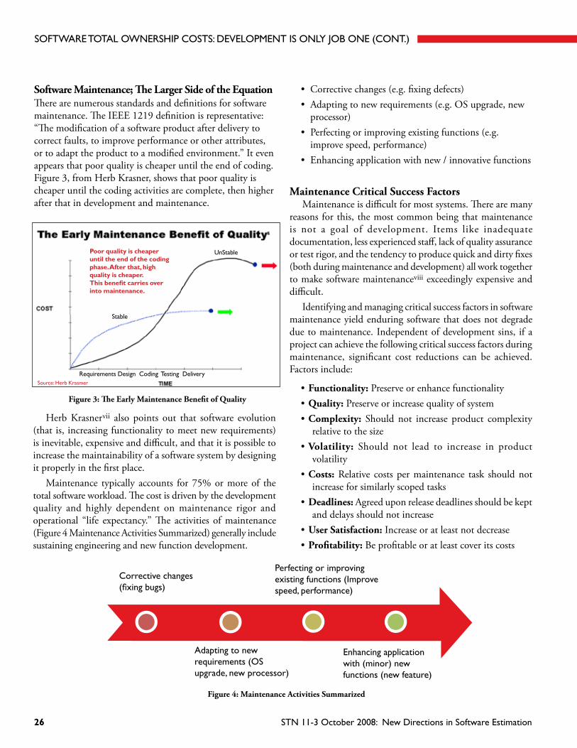
Herb Krasnervii also points out that software evolution (that is, increasing functionality to meet new requirements) is inevitable, expensive and difficult, and that it is possible to increase the maintainability of a software system by designing it properly in the first place.

Maintenance typically accounts for 75% or more of the total software workload. The cost is driven by the development quality and highly dependent on maintenance rigor and operational “life expectancy.” The activities of maintenance (Figure 4 Maintenance Activities Summarized) generally include sustaining engineering and new function development.

• Correctivechanges(e.g.fixingdefects)• Adaptingtonewrequirements(e.g.OSupgrade,new

processor)• Perfectingorimprovingexistingfunctions(e.g.

improve speed, performance)• Enhancingapplicationwithnew/innovativefunctions

Maintenance Critical Success FactorsMaintenance is difficult for most systems. There are many

reasons for this, the most common being that maintenance is not a goal of development. Items like inadequate documentation, less experienced staff, lack of quality assurance or test rigor, and the tendency to produce quick and dirty fixes (both during maintenance and development) all work together to make software maintenanceviii exceedingly expensive and difficult.

Identifying and managing critical success factors in software maintenance yield enduring software that does not degrade due to maintenance. Independent of development sins, if a project can achieve the following critical success factors during maintenance, significant cost reductions can be achieved. Factors include:

•Functionality: Preserve or enhance functionality •Quality: Preserve or increase quality of system •Complexity: Should not increase product complexity

relative to the size •Volatility: Should not lead to increase in product

volatility •Costs: Relative costs per maintenance task should not

increase for similarly scoped tasks •Deadlines: Agreed upon release deadlines should be kept

and delays should not increase •User Satisfaction: Increase or at least not decrease •Profitability: Be profitable or at least cover its costs

Software Maintenance; The Larger Side of the EquationThere are numerous standards and definitions for software maintenance. The IEEE 1219 definition is representative: “The modification of a software product after delivery to correct faults, to improve performance or other attributes, or to adapt the product to a modified environment.” It even appears that poor quality is cheaper until the end of coding. Figure 3, from Herb Krasner, shows that poor quality is cheaper until the coding activities are complete, then higher after that in development and maintenance.

Figure 3: The Early Maintenance Benefit of Quality

Figure 4: Maintenance Activities Summarized


corrective changes (fixing bugs)

perfecting or improving existing functions (Improve speed, performance)

Enhancing application with (minor) new functions (new feature)

Adapting to new requirements (OS upgrade, new processor)

requirements Design coding Testing Delivery

Poor quality is cheaper until the end of the coding phase. After that, high quality is cheaper.This benefit carries over into maintenance.

Stable

UnStable

Source: herb Krasmer


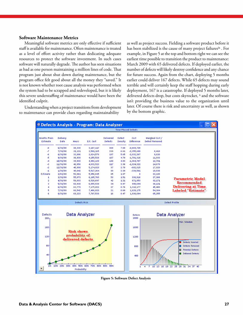
Software Maintenance Metrics Meaningful software metrics are only effective if sufficient

staff is available for maintenance. Often maintenance is treated as a level of effort activity rather than dedicating adequate resources to protect the software investment. In such cases software will naturally degrade. The author has seen situations as bad as one person maintaining a million lines of code. That program just about shut down during maintenance, but the program office felt good about all the money they “saved.” It is not known whether root cause analysis was performed when the system had to be scrapped and redeveloped, but it is likely this severe understaffing of maintenance would have been the identified culprit.

Understanding when a project transitions from development to maintenance can provide clues regarding maintainability

as well as project success. Fielding a software product before it has been stabilized is the cause of many project failuresix . For example, in Figure 5 at the top and bottom right we can see the earliest time possible to transition the product to maintenance: March 2009 with 65 delivered defects. If deployed earlier, the number of defects will likely destroy confidence and any chance for future success. Again from the chart, deploying 5 months earlier could deliver 167 defects. While 65 defects may sound terrible and will certainly keep the staff hopping during early deployment, 167 is a catastrophe. If deployed 5 months later, delivered defects drop, but costs skyrocket, x and the software isn’t providing the business value to the organization until later. Of course there is risk and uncertainty as well, as shown by the bottom graphic.

Figure 5: Software Defect Analysis


These are examples of metrics that may identify what we are doing that we should not and/or what we are not doing that we should:

• Numberofnewdefectscreatedbyfixes• Number of defect corrections thatwere not correct

(Defective)• Number of defects not repaired in promised time

(Delinquent)• DefectSeepage(Customerreporteddefectsduringpre-

delivery testing)

Maintenance Productivity DriversWhen looking at software maintenance costs, the sins or

blessings of development come into play, plus a number of other items that help scope maintenance.

Years of Maintenance: Number of years for which software maintenance costs will be estimated (Maintenance typically begins when operational test & evaluation is completed).

Separate Sites: Number of separate operational sites where the software will be installed and users will have an input into system enhancements (Only sites that have some formal input, not necessarily all user sites). More sites = more enhancing, corrective, and perfective effort

Maintenance Growth Over Life: Anticipated size growth from the point immediately after the software is turned over to maintenance through the end of the product life cycle. This includes additions of innovations and other functionality. Figure 6 illustrates development versus maintenance growth.

0500

100015002000250030003500

Hours By Month

Development

Figure 6: Development Vs Maintenace 0 Growth


• Defectsremovedperunittime• Productivityforblockchanges• Meantimetofindthenextkfaults• Maintenancebacklog• Increases/decreaseonmaintenancebacklog• Numberoftroublereportsopenedandclosed• Meantimeuntilproblemclosed• Defectsduringwarrantyperiod• Meantimetoresolution

• Defectsbytypeandseverity• Timetorespondtocustomerreporteddefects• McCabe&Halsteadcomplexitymetricsxi • SoftwareMaturityIndex(IEEE982Standard

Dictionary of Measures To Produce Reliable Software) M = number of modules in current version A = number of added modules in current version C = number of changed modules in current version D = number of deleted modules in current version

compared to the previous version SoftwareMaturityIndex = (M - (A + C + D)) / M

Example Maintenance Metrics

Example Maintenance Effectiveness Metrics

When the Software Maturity Index approaches 1.0 the product is stable. Unfortunately, in many domains, it is likely old enough to be approaching retirement at this point.

Generally, you get what you measure. Choosing the right metrics for your project is a key consideration. The following identifies some of the possible traditional appropriate maintenance metrics:


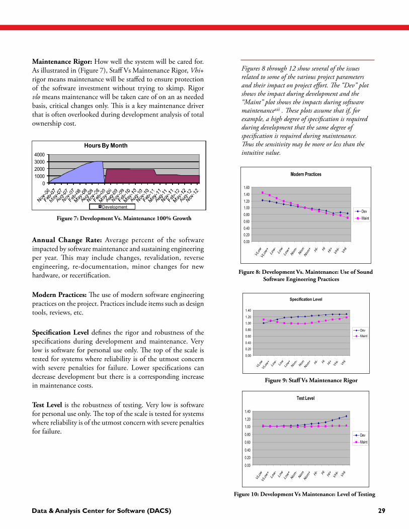
01000200030004000

Hours By Month

Development

Figure 7: Development Vs. Maintenance 100% Growth

Maintenance Rigor: How well the system will be cared for. As illustrated in (Figure 7), Staff Vs Maintenance Rigor, Vhi+ rigor means maintenance will be staffed to ensure protection of the software investment without trying to skimp. Rigor vlo means maintenance will be taken care of on an as needed basis, critical changes only. This is a key maintenance driver that is often overlooked during development analysis of total ownership cost.

Annual Change Rate: Average percent of the software impacted by software maintenance and sustaining engineering per year. This may include changes, revalidation, reverse engineering, re-documentation, minor changes for new hardware, or recertification.

Modern Practices: The use of modern software engineering practices on the project. Practices include items such as design tools, reviews, etc.

Specification Level defines the rigor and robustness of the specifications during development and maintenance. Very low is software for personal use only. The top of the scale is tested for systems where reliability is of the utmost concern with severe penalties for failure. Lower specifications can decrease development but there is a corresponding increase in maintenance costs.

Test Level is the robustness of testing. Very low is software for personal use only. The top of the scale is tested for systems where reliability is of the utmost concern with severe penalties for failure.

Figures 8 through 12 show several of the issues related to some of the various project parameters and their impact on project effort. The “Dev” plot shows the impact during development and the “Maint” plot shows the impacts during software maintenancexii . These plots assume that if, for example, a high degree of specification is required during development that the same degree of specification is required during maintenance. Thus the sensitivity may be more or less than the intuitive value.

Figure 8: Development Vs. Maintenance: Use of Sound Software Engineering Practices

Modern Practices

0.000.200.400.600.801.001.201.401.60

VLow

VLow

+Lo

w- Low

Low+

Nom-

Nom

Nom+ Hi

- Hi Hi+

VHi-

VHi

DevMaint

Figure 9: Staff Vs Maintenance Rigor

Specification Level

0.00

0.20

0.40

0.60

0.80

1.00

1.20

1.40

VLow

VLow+

Low-

Low

Low+

Nom-

NomNom

+ Hi- HiHi+

VHi-VHi

DevMaint

Test Level

0.00

0.20

0.40

0.60

0.80

1.00

1.20

1.40

VLow

VLow

+Lo

w- Low

Low+

Nom-

Nom

Nom+ Hi

- Hi Hi+

VHi-

VHi

DevMaint

Figure 10: Development Vs Maintenance: Level of Testing


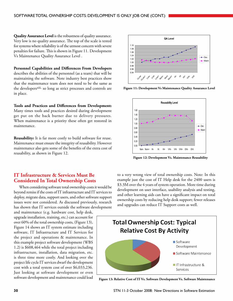
Quality Assurance Level is the robustness of quality assurance. Very low is no quality assurance. The top of the scale is tested for systems where reliability is of the utmost concern with severe penalties for failure. This is shown in Figure 11. Development Vs Maintenance Quality Assurance Level .

Personnel Capabilities and Differences From Developers describes the abilities of the personnel (as a team) that will be maintaining the software. Note industry best practices show that the maintenance team does not need to be the same as the developersxiii, so long as strict processes and controls are in place.

Tools and Practices and Differences from Development: Many times tools and practices desired during development get put on the back burner due to delivery pressures. When maintenance is a priority these often get restored in maintenance.

Reusability: It is far more costly to build software for reuse. Maintenance must ensure the integrity of reusability. However maintenance also gets some of the benefits of the extra cost of reusability, as shown in Figure 12.


QA Level

0.940.960.981.001.021.041.061.081.10

VLow

VLow+

Low-

Low

Low+

Nom-

NomNom

+ Hi- HiHi+

VHi-VHi

DevMaint

Figure 11: Development Vs Maintenance Quality Assurance Level

Figure 12: Development Vs. Maintenance Reusability

Reusability Level

0.00

0.20

0.40

0.60

0.80

1.00

1.20

1.40

1.60

Nom Nom+ Hi- Hi Hi+ VHi- VHi VHi+ EHi- EHi

DevMaint

IT Infrastructure & Services Must Be Considered In Total Ownership Costs

When considering software total ownership costs it would be beyond remiss if the costs of IT infrastructure and IT services to deploy, migrate data, support users, and other software support issues were not considered. As discussed previously, research has shown that IT services outside the software development and maintenance (e.g. hardware cost, help desk, upgrade installation, training, etc.) can account for over 60% of the total ownership costs, (Figure 13), Figure 14 shows an IT system estimate including software, IT Infrastructure and IT Services for the project and operations & maintenance. In this example project software development (WBS 1.2) is $608,464 while the total project including infrastructure, installation, data migration, etc. is three time more costly. And looking over the project life cycle IT services dwarf the development cost with a total system cost of over $6,033,236. Just looking at software development or even software development and maintenance could lead

to a very wrong view of total ownership costs. Note: In this example just the cost of IT Help desk for the 2400 users is $3.3M over the 4 years of system operation. More time during development on user interface, usability analysis and testing, and other learning aids can have a significant impact on total ownership costs by reducing help desk support; fewer releases and upgrades can reduce IT Support costs as well.

Figure 13: Relative Cost of IT Vs. Software Development Vs. Software Maintenance


Figure 14: Example IT Support Costs For An Application

Generating an EstimateFor software, appropriate estimation can actually impact total

ownership costs, as decisions are made based on estimates of both development and maintenance costs. It is important to optimize both of these areas. However, while development equations for SEER®, COCOMO, and other software development models are fairly well known, maintenance equations are not.

SEER for Software, for example uses sophisticated software total ownership model modeling including all the information from development (people, process, technology, defects, scope, etc.) and specifics about the maintenance such as the rigor and amount of the software to be maintained.

Figure 15. Maintenance Staffing Plus Block Changes, illustrates how maintenance is often higher in the early years than later, assuming the system remains relatively stable. Of course, block changes, major changes with significant functionality (innovation) often occur, causing increases in staffing. Those block changes are often estimated and managed as enhancements to existing systems, in addition to the maintenance.

The following equationiii (simplified to fit the scope of this paper) approximates the steady state (staff) maintenance (when the maintenance flattens):

SteadyStateMainteanceStaff Level =

0.393469 x (Complexity)-0.35 x ((MaintSize)/MaintCte)1.2 x MaintQuality

Complexity ranges from 28(vlo-) to 4 (ehi+), so complexity-.35 increases from 0.31 to 0.61 as you increase complexityMaintSize is how much of the system size must be maintained, usually total size, but can be effective size, adjusted from maintenance growth, change and sites.MaintCte is the effective technology rating (People, Process, Products) using the maintenance sensitivitiesMaintQuality is “Maintenance Rigor”which ranges from 0.6 to 1.2

Figure 15: Maintenance Staffing Plus Block Changes


Block Change Staff Levels

Maintenance Staff Levels


Also a classic rough order of magnitude rule of thumb from Barry Boehm’s original COCOMO for determining annual maintenance effort can also be useful:

Annual Maintenance Effort = (Annual Change Rate)* (Original Software Development Effort)

The quantity Original Software Development Effort refers to the total effort (person-months or other unit of measure) expended throughout development, even if a multi-year project.

The multiplier Annual Change Rate is the proportion of the overall software to be modified during the year. This is relatively easy to obtain from engineering estimates. Developers often maintain change lists, or have a sense of proportional change to be required even before development is complete.

In SummaryDevelopment decisions, processes and tools can have a

significant impact on maintenance and total ownership costs. These software maintenance costs can be 75% of software total ownership costs while IT infrastructure can add another 60% on top of software. Estimation / planning processes, measurement and analysis and monitoring and control can both reduce costs themselves and can point to the areas and decisions that can reduce total ownership costs. Treating software maintenance as a level of effort activity has consequences in quality, functionality and reliability as well as costs. Applied measurement is a critical component of software and systems management.

Apply estimation techniques to determine the cost, effort, schedule, risk, stakeholder satisfaction of spending a bit more in development to reduce maintenance and total ownership costs. Apply estimation and planning, measurement and analysis, and monitoring and control to develop and maintain software with sufficient documentation and quality to optimize total costs of ownership.

About The AuthorDuring his over three decades in the industry,

Daniel D. Galorath of Galorath Inc., has been solving a variety of management, costing, systems, and software problems for both information technology and embedded systems. He has performed all aspects of software development and software management. One of his strengths has been reorganizing troubled software projects, assessing their progress, applying methodology and plans for completion and estimated cost to complete. He has personally managed some of these projects to successful completion. He has created and implemented software management policies, and reorganized (as well as

designed and managed) development projects. He is founder and CEO of Galorath Incorporated, which has developed the SEER application for Software, Hardware, Electronics & Systems, Manufacturing, and Information Technology: cost, schedule, and risk analysis, and management decision support. He was one of the principal architects of SEER for Software (SEER-SEM) cost, schedule, risk, reliability estimation model. His teaching experience includes development and presentation of courses in Software Cost, Schedule, and Risk Analysis; Software Management; Software Engineering; and Weapons Systems Architecture. Mr. Galorath has lectured internationally. Among Mr. Galorath’s published works are papers encompassing software cost modeling, testing theory, software life cycle error prediction and reduction, and software and systems requirements definition. Mr. Galorath was named winner of the 2001 International Society of Parametric Analysts (ISPA) Freiman Award, awarded to individuals who have made outstanding contributions to the theoretical or applied aspects of parametric modeling. Mr Galorath’s book, “Software Sizing, Estimation, and Risk Management” was published in March 2006. His blog may be found at www.galorath.com/wp

Author Contact InformationDan Galorath: [email protected]

ReferencesiGartnerGroup, IT Worldwide Spending, http://www.gartner.com/

it/page.jsp?id=742913, July 2008.iiMore projects fail due to lack of planning… find references.iiiGalorath, D, Evans, M, Software Sizing, Estimation and Risk Management, Auerbach Publications, 2006

ivGoldratt,E., Theory of Constraints, North River Press, 1999.vGalorath Incorporates, SEER for IT User Guide, 2008.viEvans, M, Abela, A, Beltz T, , even Characteristics of Dysfunctional

Software Projects, Crosstalk, 2002viiKrasner, Herb, The ROI of Software Evolution and Maintenance

Best Practices: Where to Find the Benefits, 2008.viiiSneed, H, Brossler, P, Critical Success Factors In Software

Maintenance: A Case Study, IEE, 2003.ixStandish Group, Chaos Report, 1998.xGalorath, D, Reifer, D, “Using Statistics To Determine How

Much Testing Is Enough”, Prepared for Naval Underwater Systems Center, Newport, RI, 1981.Reifer, Galorath…. When should you stop testing.. finish reference.

xiIEEE, IEEE Standard for Software Quality Assurance, , IEEE Std 730-2002, 2002.

xiiGalorath Incorporated, SEER for Software User Guide, 2008. Tony Salvaggio, Compaid CEO Briefing, 2008.


Including Risk Analysis in Software Cost Estimatesin spite of the fact that their outputs may not alWays be believed, modern softWare cost estimating tools are noW capable of serving a variety of important project management functions.by capers Jones, president, capers Jones & Associates LLc

Software has a bad reputation as a troubling technology. Large software projects have a very high frequency of schedule overruns, cost overruns, quality problems,

and outright cancellations. If the software is developed under contract by an outsource vendor, many of these problems end up in court for breach of contract.

From studies carried out by the author and his colleagues, manual estimates by project managers tend to be more optimistic than automated estimates carried out by commercial estimating tools such as COCOMO II, CostExpert, KnowledgePlan, Price-S, SEER, SLIM, and a number of others. The reason for this is that commercial software estimating tools are pre-loaded with substantial volumes of historical data. Commercial estimating tools don’t “forget” to include activities such as user documents. They also use historical data for dealing with critical activities such as test schedules.

In some lawsuits, depositions and testimony reveal the surprising fact that accurate estimates were prepared using automated tools, but the estimates were rejected by top executives or clients. In place of the original estimates, the project managers were ordered to meet arbitrary schedules and costs established by clients based on external business needs rather than team capabilities.

This situation brings up one of the first risks of software applications: accurate estimates may not be believed. The best solution to this problem is to support the estimate by large volumes of historical benchmark data.

In spite of the fact that their outputs may not always be believed, modern software cost estimating tools are now capable of serving a variety of important project management functions. In addition, the accuracy and precision of such tools is now high enough to merit their use for business agreements such as contracts and outsource agreements.

Three Fundamental Equations of Software EstimatingAlthough software cost estimating is a very difficult intellectual

problem, there are three fundamental equations that are rather straightforward. These equations make use of important estimating concepts that are linked together for estimation: 1) assignment scopes, 2) production rates, 3) schedules.

The “assignment scope” is the amount of some kind of work

for which one person will normally be responsible. Assignment scopes can be expressed in terms of natural metrics such as pages of specifications or lines of code. However assignment scopes can also be expressed in terms of synthetic metrics such as function points. The use of function point metrics allows all activities to be estimated using a single metric.

The “production rate” is the amount of work which one person can complete in a given time period such as an hour, a day, a week, a month, or a year. Here too either natural or synthetic metrics can be used.

The schedule of an activity or task is the amount of calendar time required to complete an activity. Schedules can be calculated by dividing the effort required for an activity by the staff available to perform it. An example can clarify the three concepts.

Suppose you are managing an application of 100,000 lines of source code using the C programming language. A typical assignment scope for an average C programmer is roughly 10,000 lines of source code, so this application might require 10 programmers.

Journeyman C programmers have average coding production rates of about 2,000 lines of source code per month, so the coding of the application will take about 50 person-months of effort.

If the effort for coding the project is 50 person-months and there are 10 programmers assigned, then the schedule for coding will be 5 calendar months.

Note that the logic of assignment scopes and production rates can be expressed in almost any metric: lines of code, function points, pages of text, test cases, or whatever. The normal sequence of applying these estimating equations is:

1. Size of deliverable / assignment scope = staff2. Size of deliverable / production rate = effort3. Effort / staff = schedule

The equations are simple in principle, but very tricky in real life. The difficulty is not in the equations themselves, but in knowing the exact assignment scopes and production rates with enough precision for the equations to yield useful results. It is the ability to adjust the fundamental equations in response


to varying degrees of staff skill, to different tools, to different methodologies, and to different programming languages that make commercial software estimating tools valuable. This same kind of information is so difficult to acquire and so valuable that the estimating tool vendors almost universally treat adjustment data as proprietary information or as trade secrets.

Nine Steps of Software Cost EstimationAll software estimating tools typically perform the eight of

the nine functions discussed here: 1) Sizing project deliverables, 2) Estimating defect levels and removal efficiency; 3) Selecting project activities; 4) Estimating staffing levels; 5) Estimating effort; 6) Estimating costs; 7) Estimating schedules; 8) Estimating requirements changes during development.

The ninth function is not always present in software cost estimation tools: risk analysis. The major risks that need to be analyzed include:

1. Outright cancellation of the project2. The odds of litigation for breach of contract3. Poor quality control4. Excessive requirements changes

We will discuss risk estimation after we have examined the eight steps in the normal sequence of estimation, although some risks are included in normal estimating steps.

Step 1: Sizing Specifications, Source Code, and Test Cases

The first step in any software estimate is to predict the sizes of the deliverables that must be constructed. Sizing must include all deliverable such as specifications, documents, and test cases as well as source code. The older software cost estimating tools such as the original COCOMO did not include sizing logic, and size information had to be provided by the user.

However, the invention of function point metrics has made full sizing logic for all deliverables a standard feature of commercial estimating tools. As of 2008, sizing is a standard feature of commercial software cost estimating tools, and a variety of sizing methods are now included, such as:

1. Sizing based on function point metrics2. Sizing based on lines of code (LOC) metrics3. Sizing based on object-oriented metrics4. Sizing based on analogy with past projects

5. Sizing based on pattern-matching6. Sizing based on attributes such as screens and

reports created

It should be noted that one very common risk with estimates based on “lines of code” metrics is that such estimates are not reliable for predicting user documents or any non-coding activity such as quality assurance, data base administration, and project management. LOC-based estimates and function point-based estimates are of approximately equal accuracy for predicting coding activities, but the LOC estimates usually are less accurate for non-code activities. Since paperwork in all of its forms is often the most expensive task for large defense applications, this problem is fairly significant. Even for civilian projects paperwork may cost more than the source code for large applications.

Step 2: Estimating Defects and Defect Removal Efficiency Levels

A key aspect of software cost estimating is predicting the time and effort that will be needed for design reviews, code inspections, and all forms of testing. In order to estimate defect removal costs and schedules, it is necessary to know about how many defects are likely to be encountered.

Poor quality control is another major risk that can lead to litigation. In every case where the author worked as an expert witness, quality control was deficient. Lack of early defect detection and removal via inspections can lead to huge delays in testing schedules. What happens is that testing might start on time, but due to the unexpected volume of defects it cannot end on time. Testing is the primary phase where schedules begin to go out of control.

The typical sequence is to estimate defect volumes for a project, and then to estimate the series of reviews, inspections, and tests that the project utilize. The defect removal efficiency of each step will also be estimated. The effort and costs for preparation, execution, and defect repairs associated with each removal activity will also be estimated.

Table 1 illustrates the overall distribution of software errors. In Table 1, bugs or defects are shown from five sources: requirements errors, design errors, coding errors, user documentation errors, and “bad fixes.” A “bad fix” is a secondary defect accidentally injected in a bug repair. In other words, a bad fix is a failed attempt to repair a prior bug that accidentally contains a new bug. On average about 7% of defect repairs will themselves accidentally inject a new defect, although the range is from less than 1% to more than 20% bad fix injections.

iNcLUDiNg riSK ANALySiS iN SOFTwArE cOST ESTiMATES (cONT.)


Table 1 presents approximate average values, but the range for each defect category is more than 2 to 1. For example, software projects developed by companies who are at level 5 on the SEI Capability Maturity Model (CMM) might have less than half of the potential defects shown in Table 1. Similarly, companies with several years of experience with the “Six Sigma” quality approach will also have lower defect potentials than those shown in Table 3. Several commercial estimating tools make adjustments for such factors.

Note that the majority of defects shown in Table 1 are not in the code itself. This is one of the reasons why LOC-based estimation is less accurate than function-point based estimation. Estimates based on lines of code cannot accurately predict bugs or defects in requirements and design, which outnumber coding defects for all large applications.

A key factor for accurate estimation involves the removal of defects via reviews, inspections, and testing. The measurement of defect removal is actually fairly straight forward, and many companies now do this. The U.S. average is about 85%, but leading companies can average more than 95% removal efficiency levels.

It is much easier to estimate software projects that use sophisticated quality control and have high levels of defect removal in the 95% range. This is because there usually are no disasters occurring late in development when unexpected defects are discovered. Thus, projects performed by companies at the higher CMM levels or by companies with extensive six-sigma experience for software often have much greater precision than average.

Step 3: Selecting Project ActivitiesOnce the size of various deliverables has been approximated

the next step is to determine which specific activities will be carried out for the project being estimated. This is one of the major areas where software cost estimating tools excel. Modern cost estimating tools can analyze the nature, size, and class of the application being estimated and automatically select the most likely set of activities.

Estimates for entire projects or for phases are not accurate enough for contracts or serious planning. Activity-based cost estimates with perhaps 20 to 25 activities are the level of precision offered by modern cost estimating tools.

Step 4: Estimating Staffing LevelsAlthough staffing, effort, costs, and

schedules are all important for the final estimate, the normal place to start estimating is with staffing levels. The fundamental equation for determining staff is:

Size of deliverable / assignment scope = staff.

Commercial software cost estimating tools apply this fundamental staffing equation in a wide variety of forms, including but not limited to:

Pages of specifications / assignment scope = analystsLines of source code / assignment scope = programmersTest cases / assignment scope = testersPages of user manuals / assignment scope = technical writers

Number of employees / assignment scope = managers

The examples just shown make use of natural metrics that define the actual material to be created such as pages or code. The staffing equation can also be used with the synthetic function point metric. In fact, the equations can be utilized with any metric if it can express the amount of work normally assigned to individual technical workers.

Step 5: Estimating Software EffortThe term “effort” defines the amount of human work

associated with a project. The amount of effort can be expressed in any desired metric, such as work hours, work days, work weeks, work months, or work years. Usually small projects of up to perhaps 1000 function points utilize “hours” for expressing effort, but the larger projects in excess of 10,000 function points normally utilize “months” as the unit of measure. The general algorithm for predicting effort is:

Size of deliverable / production rate = staff effort

Here too this basic equation is used in a variety of forms including but not limited to:

Pages of specifications / production rate = analyst monthsLines of source code / production rate = programmer months


Test cases / production rate = testing monthsDefects found / production rate = rework monthsPages of user manuals / production rate = writing months

Note also that the use of “months” in this example is simply to indicate a work period. Estimates can be expressed in terms of work hours, work weeks, work months, or even work years.

Some typical examples of these rules are as follows: Specifications are normally prepared at a rate of about 20 pages per analyst month while technical writing proceeds at a rate of about 50 pages per month. Coding takes place at a rate of about 1000 source code statements per month. Here, too, there are very broad ranges and so average values need to be adjusted to match the actual project and team characteristics.

For any given software activity, the measured range between the best performance and the worst performance is about 1000%. This is far too broad a range for “average” values to be useful for serious estimation. Therefore, knowledge of how to adjust production rates in response to various factors is the true heart of software estimation.

Step 6: Estimating Software CostsThe fundamental equation for estimating the cost of a software

activity is simple in concept, but very tricky in real life:

Effort * (salary + burden) = cost

One basic problem is that software staff compensation levels vary by about a ratio of 3 to 1 in the United States, and by more than 10 to 1 when considering global compensation levels for any given job category. For example, here in the United States there are significant ranges in average compensation by industry and also by geographic region. Programmers in a large bank in mid-town Manhattan or San Francisco will average more than $80,000 per year, but programmers in a retail store environment in the rural south might average less than $55,000 per year.

With cost ranges such as those for projects that took exactly the same amount of programming staff effort, it is easy to see why figures such as “average cost per function point” should not be used without substantial adjustments for local conditions.

Step 7: Estimating Software SchedulesThe fundamental equation for estimating the schedule of

any given software development activity is:

Effort / staff = time period

Using this equation, an activity that requires eight person-months of effort and has four people assigned to it can be finished in two calendar months; i.e. 8 months / 4 people = 2 calendar months.

However, in real life, schedule estimating is one of the most difficult parts of the software estimation process and many highly complex topics must be dealt with, such as:

• Dependenciesofoneactivityuponprevious activities

• Overlaporconcurrencyofactivities• Thecriticalpaththroughthesequenceofactivities• Lessthanfull-timeavailabilityofstaff• Numberofshiftsworkedperday• Numberofeffectiveworkhourspershift• Paidorunpaidovertimeappliedtotheactivity• Interruptionssuchastravel,meetings,training,or

illness

Incidentally, there are two main reasons for schedule slippages on large software applications: 1) Excessive defect volumes that do not appear until testing begins or even in the midst of testing; 2) Significant volumes of requirements changes that were not planned for or included in the schedules.

Step 8: Estimating Requirements Changes During Development

One important aspect of estimating is dealing with the rate at which requirements “creep” and hence make projects grow larger during development. Fortunately, function point metrics allow direct measurement of the rate at which this phenomenon occurs, since both the original requirements and changed requirements will have function point counts.

Changing requirements can occur at any time, but the data in Table 2 runs from the end of the requirements phase to the beginning of the coding phase. This time period usually reflects about half of the total development schedule. Table 2, shows the approximate monthly rate of creeping requirements for six kinds of software, and the total volume of change that might be anticipated:

For estimates made early in the life cycle, several estimating tools can predict the probable growth in unplanned functions over the remainder of the development cycle. This knowledge can then be used to refine the estimate, and to adjust the final costs in response.



Of course, the best response to an estimate with a significant volume of projected requirements change is to improve the requirements gathering and analysis methods. Thus projects that use prototypes, joint application design (JAD), requirements inspections, and other sophisticated requirements methods can reduce later changes down to a small fraction of the values shown in Table 2. Indeed, the initial estimates made for projects using JAD will predict reduced volumes of changing requirements.

Step 9: Software Risk AnalysisThe software industry has long been troubled by major

schedule slippage, major cost overruns, and a high incidence of outright failure.

Table 3 shows the approximate frequency of various kinds of outcomes, based on the overall size of the project being attempted. Table 3 is taken from the author’s book, Patterns of Software Systems Failure and Success (International Thomson Press, 1995).

As can easily be seen from Table 3, small software projects are successful in the majority of instances, but the risks and hazards of cancellation or major delays rise quite rapidly as the overall application size goes up. Indeed, the development of large applications in excess of 10,000 function points is one of the most hazardous and risky business undertakings of the modern world.

Of all the troublesome factors associated with software, schedule slips stand out as being the most frequent source of litigation between outsource vendors and their clients. Schedule slips are also the main reason for executive frustration with software for internal projects.

Fortunately, as of 2008, objective empirical data is beginning to become available in significant quantities. The International Software Benchmark Standards Group (ISBSG) was founded in 1997. Now that it has been operational for more than 10 years, the volume of measured historical data has reached about 5,000 software projects.

Besides ISBSG there are a number of software benchmark data bases, but these are usually proprietary and not generally available. Some of this data is generally available in books such

as the author’s Applied Software Measurement (McGraw Hill, 2008), Software Assessments, Benchmarks, and Best Practices (Addison Wesley 2000), and Estimating Software Costs (McGraw Hill 2007).

Estimating the Risk and Costs of Canceling Large Software Applications

For applications larger than 10,000 function points in size, cancellation occurs with alarming frequency as shown in Table 4. The most troubling aspect of cancelled projects is the fact that the projects are usually late and over budget at the time of cancellation. On average, cancelled projects cost about 15% more than successful projects of the same size.

Since successful applications in the 10,000 function point size range cost about $2,000 per function point, it is a serious waste of corporate funds that cancelled projects average about $2,300 per function point. Larger applications cost even more.

Estimating the Risk and Costs of LitigationWhen internal projects are cancelled, money is wasted and

sometimes people are fired, but the situation does not end up in court. When projects done by outsource vendors or contractors are cancelled, the situation often does end up in court. Table 4 shows the approximate results of U.S. outsource agreements:

In performing “autopsies” of cancelled or failed projects it is fairly easy to isolate the attributes that distinguish disasters from successes. Experienced project managers know that false optimism in estimates, failure to plan for changing requirements, and inadequate quality approaches lead to failures and disasters. Conversely, accurate estimates, careful change control, and top-notch quality control are stepping stones to success.

If a cancelled project does end up in court, both parties can look forward to about 36 months of expensive litigation, unless they settle out of court. For an application of 10,000 function points in size, the plaintiff can expect to spend at least $5,000,000 in legal fees and expert witness costs. This is about


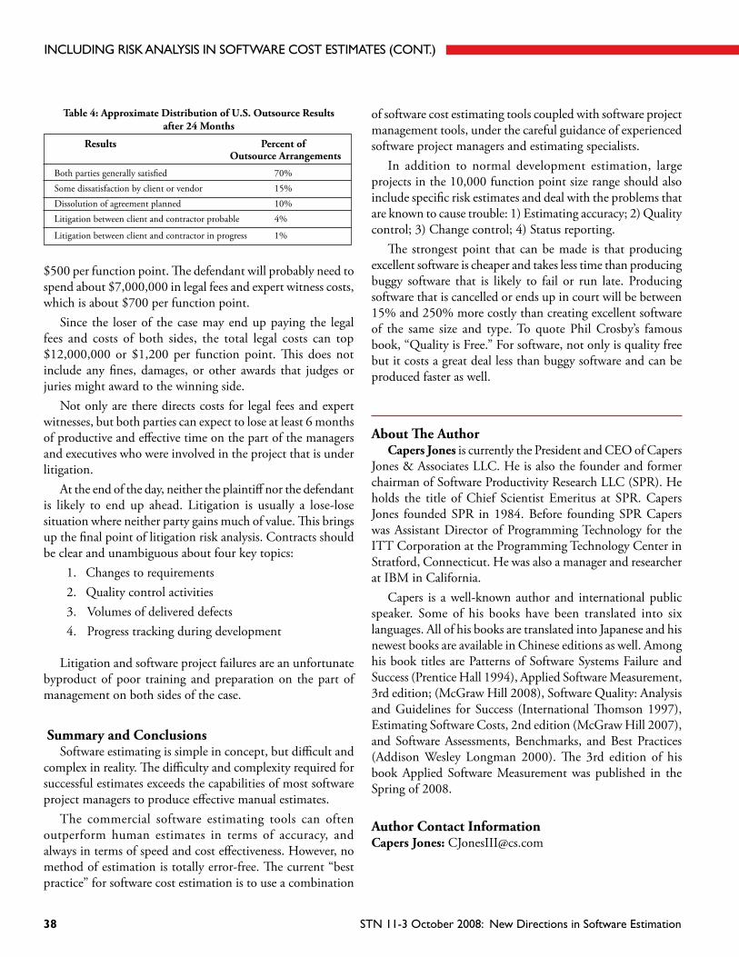
$500 per function point. The defendant will probably need to spend about $7,000,000 in legal fees and expert witness costs, which is about $700 per function point.

Since the loser of the case may end up paying the legal fees and costs of both sides, the total legal costs can top $12,000,000 or $1,200 per function point. This does not include any fines, damages, or other awards that judges or juries might award to the winning side.

Not only are there directs costs for legal fees and expert witnesses, but both parties can expect to lose at least 6 months of productive and effective time on the part of the managers and executives who were involved in the project that is under litigation.

At the end of the day, neither the plaintiff nor the defendant is likely to end up ahead. Litigation is usually a lose-lose situation where neither party gains much of value. This brings up the final point of litigation risk analysis. Contracts should be clear and unambiguous about four key topics:

1. Changes to requirements2. Quality control activities3. Volumes of delivered defects4. Progress tracking during development

Litigation and software project failures are an unfortunate byproduct of poor training and preparation on the part of management on both sides of the case.

Summary and ConclusionsSoftware estimating is simple in concept, but difficult and

complex in reality. The difficulty and complexity required for successful estimates exceeds the capabilities of most software project managers to produce effective manual estimates.

The commercial software estimating tools can often outperform human estimates in terms of accuracy, and always in terms of speed and cost effectiveness. However, no method of estimation is totally error-free. The current “best practice” for software cost estimation is to use a combination

of software cost estimating tools coupled with software project management tools, under the careful guidance of experienced software project managers and estimating specialists.

In addition to normal development estimation, large projects in the 10,000 function point size range should also include specific risk estimates and deal with the problems that are known to cause trouble: 1) Estimating accuracy; 2) Quality control; 3) Change control; 4) Status reporting.

The strongest point that can be made is that producing excellent software is cheaper and takes less time than producing buggy software that is likely to fail or run late. Producing software that is cancelled or ends up in court will be between 15% and 250% more costly than creating excellent software of the same size and type. To quote Phil Crosby’s famous book, “Quality is Free.” For software, not only is quality free but it costs a great deal less than buggy software and can be produced faster as well.

About The AuthorCapers Jones is currently the President and CEO of Capers

Jones & Associates LLC. He is also the founder and former chairman of Software Productivity Research LLC (SPR). He holds the title of Chief Scientist Emeritus at SPR. Capers Jones founded SPR in 1984. Before founding SPR Capers was Assistant Director of Programming Technology for the ITT Corporation at the Programming Technology Center in Stratford, Connecticut. He was also a manager and researcher at IBM in California.

Capers is a well-known author and international public speaker. Some of his books have been translated into six languages. All of his books are translated into Japanese and his newest books are available in Chinese editions as well. Among his book titles are Patterns of Software Systems Failure and Success (Prentice Hall 1994), Applied Software Measurement, 3rd edition; (McGraw Hill 2008), Software Quality: Analysis and Guidelines for Success (International Thomson 1997), Estimating Software Costs, 2nd edition (McGraw Hill 2007), and Software Assessments, Benchmarks, and Best Practices (Addison Wesley Longman 2000). The 3rd edition of his book Applied Software Measurement was published in the Spring of 2008.

Author Contact InformationCapers Jones: [email protected]


Results Percent of Outsource Arrangements

Both parties generally satisfied 70%Some dissatisfaction by client or vendor 15%Dissolution of agreement planned 10%Litigation between client and contractor probable 4%

Litigation between client and contractor in progress 1%

Table 4: Approximate Distribution of U.S. Outsource Results after 24 Months


References and ReadingsCharette, Bob; Software Engineering Risk Analysis and

Management; McGraw Hill, New York, NY; 1989.Charette, Bob; Application Strategies for Risk Management;

McGraw Hill, New York, NY; 1990.Crosby, Phil; Quality is Free; Mentor Executive Library, New

York, NY; 1979.DeMarco, Tom; Controlling Software Projects; Yourdon Press,

New York; 1982; ISBN 0-917072-32-4; 284 pages.Ewusi-Mensah, Kweku; Software Development Failures; MIT

Press, Cambridge, MA; 2003; ISBN 0-26205072-2276 pages.

Galorath, Dan; Software Sizing, Estimating, and Risk Management: When Performance is Measured Performance Improves; Auerbach Publishing, Philadelphia; 2006; ISBN 10: 0849335930; 576 pages.

Garmus, David and Herron, David; Function Point Analysis – Measurement Practices for Successful Software Projects; Addison Wesley Longman, Boston, MA; 2001; ISBN 0-201-69944-3;363 pages.

Gilb, Tom and Graham, Dorothy; Software Inspections; Addison Wesley, Reading, MA; 1993; ISBN 10: 0201631814.

Glass, R.L.; Software Runaways: Lessons Learned from Massive Software Project Failures; Prentice Hall, Englewood Cliffs; 1998.

Johnson, James et al; The Chaos Report; The Standish Group, West Yarmouth, MA; 2000 (produced annually).

Jones, Capers; Applied Software Measurement; McGraw Hill, 3rd edition 2008; ISBN 978-0-07-150244-3; 575 pages; 3rd edition due in the Spring of 2008.

Jones, Capers; Assessment and Control of Software Risks; Prentice Hall, 1994; ISBN 0-13-741406-4; 711 pages.

Jones, Capers; Patterns of Software System Failure and Success; International Thomson Computer Press, Boston, MA; December 1995; 250 pages; ISBN 1-850-32804-8; 292 pages.

Jones, Capers; Software Quality – Analysis and Guidelines for Success; International Thomson Computer Press, Boston, MA; ISBN 1-85032-876-6; 1997; 492 pages.

Jones, Capers; Estimating Software Costs; McGraw Hill, New York; 2007; ISBN 13-978-0-07-148300-1.

Jones, Capers; Software Assessments, Benchmarks, and Best Practices; Addison Wesley Longman, Boston, MA; ISBN 0-201-48542-7; 2000; 657 pages.

Jones, Capers: “Sizing Up Software;” Scientific American Magazine, Volume 279, No. 6, December 1998; pages 104-111.

Jones, Capers; Conflict and Litigation Between Software Clients and Developers; Software Productivity Research, Inc.; Narragansett, RI; 2008; 45 pages.

Jones, Capers; “Preventing Software Failure: Problems Noted in Breach of Contract Litigation”; Capers Jones & Associates, Narragansett, RI; 2008; 25 pages.

Kan, Stephen H.; Metrics and Models in Software Quality Engineering, 2nd edition; Addison Wesley Longman, Boston, MA; ISBN 0-201-72915-6; 2003; 528 pages.

Radice, Ronald A.; High Qualitiy Low Cost Software Inspections; Paradoxicon Publishingl Andover, MA; ISBN 0-9645913-1-6; 2002; 479 pages.

Wiegers, Karl E.; Peer Reviews in Software – A Practical Guide; Addison Wesley Longman, Boston, MA; ISBN 0-201-73485-0; 2002; 232 pages.

Yourdon, Ed; Death March - The Complete Software Developer’s Guide to Surviving “Mission Impossible” Projects; Prentice Hall PTR, Upper Saddle River, NJ; ISBN 0-13-748310-4; 1997; 218 pages.

Yourdon, Ed; Outsource: Competing in the Global Productivity Race; Prentice Hall PTR, Upper Saddle River, NJ; ISBN 0-13-147571-1; 2005; 251 pages.



The first 50 people to send in a completed survey will receive a FREE DoD/IT Acronym CD from the DACS.

This valuable cD-rOM contains over 9,000 Department of Defense and information Technology acronyms. There are hundreds of acronym lists available but none are as well done as this CD AND specifically targeted towards DoD and Information Technology. This unique-shaped cD-rOM plays in your computer’s regular, hub-mounted, cD drive. you’ll use this great resource over and over again. It’s FREE, just for filling out our brief survey on the next page!

fold here

fold here

http://iac.dtic.mil/dacs/

Data & Analysis center for Software (DAcS)


STN Vol. 11, No. 3 October 2008 New Directions in Software Estimation

SOFTwArE TEch NEwS FEEDBAcK

1. which volume of the Software Tech News did you receive? __________________________________________

2. when did you receive the newsletter? (month/year) _______________________________________________

3. How satisfied were you with the CONTENT of the newsletter? (Article Quality) Very Satisfied Satisfied Neither Satisfied nor Dissatisfied Dissatisfied Very Dissatisfied

4. How satisfied were you with the APPEARANCE of the newsletter? Very Satisfied Satisfied Neither Satisfied nor Dissatisfied Dissatisfied Very Dissatisfied

5. How satisfied were you with the OVERALL QUALITY of the newsletter? Very Satisfied Satisfied Neither Satisfied nor Dissatisfied Dissatisfied Very Dissatisfied

6. How satisfied were you with the ACCURACY of the address on the newsletter? Very Satisfied Satisfied Neither Satisfied nor Dissatisfied Dissatisfied Very Dissatisfied

7. Approximately how much of the newsletter do you read? The entire issue Most of the content About half the content Briefly Skimmed Didn’t read

8. would you read this newsletter in an E-mail newsletter format? Definitely probably Not Sure probably Not Definitely Not

9. how did you request the product or service? phone call E-mail DAcS website Subscription Form Other ______________________

10. would you recommend the Software Tech News to a colleague? Definitely probably Not Sure probably Not Definitely Not

11. what topics would you like to see this newsletter devoted to? _____________________________________

_____________________________________________________________________________________

comments (optional) _____________________________________________________________________

_____________________________________________________________________________________

rEgiSTEr FOr ThE FirST TiME | UpDATE cUrrENT SUBScripTiON

Name: ___________________________________________ position/Title: __________________________

Organization: ______________________________________ Office Symbol: __________________________

Address: __________________________________________ city: _________________________________

State: ___________________zip: _______________ country: ______________________________________

Telephone: _____ - ______ - _______Fax: _____ - ______ - _______ Email: _______________________

Functional role: __________________________________________________________________________

Organization Type: Air Force Army Navy Other DoD _______________________________________ commercial Non-Profit Non-US US government FFr&D Other ____________

*note: you must give us your address to receive the cd. STN 11-3 October 2008: New Directions in Software Estimation42

DACS P.O. Box 1400

rome, Ny 13442-1400 Phone: 800-214-7921 Fax: 315-838-7130 E-mail: [email protected] URL: http://www.thedacs.com/

STN EDiTOriAL BOArD

Ellen Walker Managing Editor

iTT corporation, DAcS

Philip King Production Editor


Paul Engelhart DACS COTR

Air Force research Lab

Morton A. Hirschberg Editorial Board Chairman Army research Lab (retired)

Thomas McGibbon DACS Director


Dr. Kenneth E. Nidiffer Software Engineering institute

Dennis Goldenson Software Engineering institute

John Scott Mercury Federal Systems

ABOUT ThiS pUBLicATiONThe Software Tech News is published quarterly by the Data & Analysis center for Software (DAcS). The DAcS is a DoD sponsored information Analysis center (iAc), administratively managed by the Defense Technical information center (DTic). The DAcS is technically managed by Air Force research Laboratory, rome, Ny and operated by iTT, Advanced Engineering and Sciences Division.

ArTicLE rEprODUcTiONimages and information presented in these articles may be reproduced as long as the following message is noted:

“This article was originally published in the Software Tech News, Vol.11, No.3 October 2008. requests for copies of the referenced newsletter may be submitted to the following address:

Philip King, production EditorData & Analysis center for SoftwareP.O. Box 1400rome, Ny 13442-1400

Phone: 800-214-7921Fax: 315-838-7130E-mail: [email protected]

An archive of past newsletters is available at www.SoftwareTechNews.com. in addition to this print message, we ask that you notify DAcS regarding any document that references any article appearing in the Software Tech News.

Distribution Statement: Unclassified and Unlimited

ADVErTiSEMENTSThe Software Tech News is now accepting advertisements for future newsletters. in addition to being seen by the thousands of people who subscribe to a paper copy, an electronic version is available at the DACS website, exposing your product, organization, or service to hundreds of thousands of additional eyes every month.

For rates and layout information contact: [email protected]

cOVEr DESigNWendy Butcher

Graphic Designer iTT corporation, DAcS

ABOUT ThE SOFTwArE TEch NEwS


Tech Views — New Directions in Software Estimationby Dan Ferens, DACS Analyst, ITT Corporation . . . . . . . . . . . . . . . . . . . . . . . . . . . . . . . . . . . . . . . . . . . . . . . . . . . . . . . . . . . . . . . . . . . . . . . . . . . . . . . . . . . . . . . . . . . . . .3-4

Modern Tools to Support DoD Software Intensive System of Systems Cost Estimationby Jo Ann Lane and Barry Boehm, University of Southern California, Center for Systems and Software Engineering . . . . .4-13

Using Parametric Software Estimates during Program Support Reviews

by Don Scott Lucero and Christopher L. Miller, Office of the Under Secretary of Defense (OUSD) . . . . . . . . . . . . . . . . . . . . . . . . . .14-17

The Evolution of Software Size: A Search for Valueby Arlene Minkiewicz, PRICE Systems LLC . . . . . . . . . . . . . . . . . . . . . . . . . . . . . . . . . . . . . . . . . . . . . . . . . . . . . . . . . . . . . . . . . . . . . . . . . . . . . . . . . . . . . . . . . . . . . . . 18-22

Software Total Ownership Costs: Development Is Only Job Oneby Daniel D. Galorath, Galorath Inc. . . . . . . . . . . . . . . . . . . . . . . . . . . . . . . . . . . . . . . . . . . . . . . . . . . . . . . . . . . . . . . . . . . . . . . . . . . . . . . . . . . . . . . . . . . . . . . . . . . . . . . . 23-32

Including Risk Analysis in Software Cost Estimatesby Capers Jones, President, Capers Jones & Associates LLC . . . . . . . . . . . . . . . . . . . . . . . . . . . . . . . . . . . . . . . . . . . . . . . . . . . . . . . . . . . . . . . . . . . . . . . . . .33-39

Data & Analysis Center for SoftwareP.O. Box 1400Rome, NY 13442-1400

PRSRT STDU.S. Postage

P A I DPermit #566

UTICA, NYReturn Service Requested

STN Vol. 11, No. 3 October 2008 New Directions in Software Estimation

iN ThiS iSSUE


Documents

2 STN 11-3 October 2008: New Directions in …such as COCOMO 2.0 in 2000), ... New Directions in Software Estimation. ... implement new features desired for SoS-level capabilities,