Embed Size (px)
Citation preview

13
2. SIMULATION AND MODELLING
Chapter overview 13
2.1. Simulation 15
2.1.1. Simulation of a complex system 15
2.1.2. Simulation development stages 19
2.1.3. Discrete Event Simulation 21
2.2. Discrete Event modelling 22
2.2.1. The logical structure of a DE model 22
2.2.2. Time flow mechanisms 24
2.2.3. The two-component functional structure 26
2.3. Simulation worldviews 27
2.3.1. The event-based worldview 28
2.3.2. The activity-scanning worldview 29
2.3.3. The process-based worldview 30
2.3.4. The three-phase worldview 31
2.4. The chapter in context 33
CHAPTER OVERVIEW
Based on a linkage of modelling and computing, simulation is used to analyse
problems by emulating the operation of the underlying systems over a period of time.
Real or hypothetical systems are modelled for some predefined purposes and used for
repeated experimentation. The intention is to understand their behaviour, so as to

CHAPTER 2 - SIMULATION AND MODELLING
14
make inferences about the system being modelled. Simulations may run through
continuous or discrete time [85]. Since it is almost never clear how detailed a model
needs to be in order to meet the intended purpose of the simulation study, successive
models are gradually built, validated, experimented through time and refined until the
final model is acceptable.
It is generally said that simulation applies where other analytical methods fail
[127], i.e. simulation methods may successfully be used to study problems of high
variability and complexity for which there are no adequate exact solutions. Instead of
adopting simplifying assumptions, simulation studies variability and complexity by
emulating the underlying system, experimenting and observing its logical and
temporal dynamics. No optimal solution will be found but a range of exploratory
scenarios and solutions can be devised [85, 101].
Simulation is neither the best nor the only technique used to tackle complex
problems. It is an alternative to direct experimentation with the real system [101, 85].
It can also be complementary to other techniques such as mathematical programming
and heuristics by providing an initial stage from which other techniques may proceed
to improve the achieved solution. Besides, it is a risk-free and legal experimental tool
that allows replication to assess the impact of new ideas, policies and rules. However,
considerable skill is needed to develop appropriate models and to apply them sensibly
and sometimes a large amount of data in specific data formats is required, which can
make it an expensive approach to use.
Simulation is not a standalone method that acts by itself. It interleaves with a wide
range of disciplines, such as information systems, statistics, modelling and computing
to structure problems and devise solutions.

CHAPTER 2 - SIMULATION AND MODELLING
15
2.1. SIMULATION
Although simulation as a management science technique dates back to the 1950’s,
there is no unique definition of its basic concepts [85]. This is probably due to the
multidisciplinary context in which it acts and interacts, where each discipline fully
defines its knowledge infrastructure. As there is no common conceptual framework, a
minimal conceptual base is provided here.
2.1.1. SIMULATION OF A COMPLEX SYSTEM
Robinson (2004) defines simulation as the “Experimentation with a simplified
imitation (on a computer) of an operations system as it progresses through time, for
the purpose of better understanding and/or improving that system.” [101]. Using C#-
based pseudo-code, this definition and the opening sentence of this chapter could be
expressed algorithmically as follow:
Algorithm SimulationHowitWorks()
Description: This is the working procedure that underlines the
above definition of simulation
{
Take the symptoms of a complex problem;
// Malfunction, lack of functionality, etc
Identify the underlying system;
// Real or hypothetical system
Build a conceptual model;
// Capturing the key features of the system
Define the experimental frame;
// Conditions under which the model is to be
observed or experimented
Do
{Build a simplified model;
// Lumped model
Implement the model;
// Computer-based system or not

CHAPTER 2 - SIMULATION AND MODELLING
16
Valid = Model(Experimental frame);
// Run the model within experimental frame}
While (Valid != “Reasonably fits the intended purpose”)
Do
{Experiment with the model over time with different policies
and rules;
// Observe the model behaviour
“What if” questions, scenarios and sensitivity analysis;
// Assess how the model behaviour is understood
Understanding=Model(scenarios);}
While (Understanding ! = “Reasonable”)
Recommendations on possible improvements;}
In all, a simulation is a system that emulates the behaviour of another system over
time [43]. It rests on the following foundational concepts:
System
A system is a purposeful collection of inter-related components working together to
achieve some common objective [116]. A system’s components can be other systems,
other components, entities, resources, jobs, events or even variables that describe the
system’s states. Systems are therefore like sets of boxes packed into successively
bigger boxes. Each component is in principle both a system and a part of a larger
system [28]. In socio-technical systems, however, the boxes are not static.
Components take purposeful actions that affect the others and vice-versa. Thus, a
system is also seen as a “set of activities linked together so that the whole set, as an
entity, could pursue a purpose” [29]. Components, while taking action, inter-relate
within the system and the system inter-relates within its super-systems. Components
in action and their interrelationships are assembled together to attain the system’s
intended purpose. An organisation and a software application alike, for example, are
sets of sub-systems in action linked together to provide some emerging whole
functionality that incorporates the functionality of each part.

CHAPTER 2 - SIMULATION AND MODELLING
17
Complexity
Systems can grow in complexity by the addition of components or new relationships
among existing components. Other aspects of complexity increase with the system’s
variability, i.e. the predictable or unpredictable variation of the components or their
interrelationships. System complexity may be classified according to the number and
nature of logical and temporal interrelationships among internal components and the
interrelationship between the system and its super systems.
Hence, combinatorial complexity results from the number of interrelationships
between components [101]. The larger the number of components and the number of
relationships, the higher is the degree of combinatorial complexity. Supply chains
systems can be, in this sense, highly complex depending on the number of suppliers,
manufacturing and distribution tiers and the number of relationships inside and across
the tiers. Fig. 2.1 shows a supply chain system with several tiers which generate a
huge number of upstream and downstream relationships.
Fig.2.1: A supply chain is potentially a combinatorial complex system due to the
number of components and interrelationships
Computational complexity derives from the algorithms required to express the
logic and the temporal interrelationships [101]. These may call for a high degree of
abstraction that generates mathematical complexity. Mathematical complexity is
reproduced in the corresponding computer programs by increasing the complexity of

CHAPTER 2 - SIMULATION AND MODELLING
18
the architecture design, the algorithms and the data structures. Considerable
processing time and space requirements will then be inevitable.
Thirdly, dynamic complexity results from the number and the nature of
interrelationships of the components through time. Communication between
components is often bidirectional: for example, in a financial system, a physical flow
may generate a financial counterpart in the reverse direction. The temporal
perturbation of these causal-effect relations due to randomly distributed delays
requires corrective actions. The synchronisation of these flows and the corrective
actions increase the complexity of the system [43].
Fig. 2.2: A supply chain is potentially a dynamic complex system due, for instance, to
the temporal effects caused by delays in the physical-financial cycles
Also, it is important to note that actions may have different effects according to
the point of time and part of the system at which they occur, and some actions have no
predictable effects [101]. Fig. 2.2 illustrates the potential dynamic complexity in a
supply chain system. A supply chain may become increasingly complex due, for
instance, to the financial flow that corresponds to the physical flow of materials.
Delays on any flow require corrective measures that may generate dynamic
complexity.

CHAPTER 2 - SIMULATION AND MODELLING
19
Finally, organisational complexity arises from the nature of the interrelationship
between the system and its external environment; that is, its super systems. This is
especially important in socio-technical systems where the human interaction with the
technical components may raise social issues that are highly unpredictable and
unquantifiable.
2.1.2. SIMULATION DEVELOPMENT STAGES
Simulation modelling and analysis is a learning process [85] that iterates through a set
of stages with the aim of understanding the behaviour of a system. Fig. 2.3 presents
the circular process of developing a simulation. This process is described in 5 stages
[85]. The pyramidal computer system inside the circle means that computers currently
provide functionalities for the development of each stage.
Fig. 2.3: Simulation development process (partly derived from Pidd, 2004)
The first stage, the conceptual model building, consists of capturing the key
features of the real or hypothetical system so that a base model can be idealised. Also,
an experimental frame [128] is set in accordance with the study purpose, to describe
the conditions within which the model is to operate. The conceptual model, explicitly
or implicitly constructed, gives way to a lumped model which is a simplified version

CHAPTER 2 - SIMULATION AND MODELLING
20
that fits the experimental frame.
The second stage, the computer implementation, consists of translating the logic
of the lumped model into a computer model. This involves a software application that
takes the lumped model description as an input, runs the simulation and allows for the
data output analysis.
These two stages run in cycles, passing from one to the other as newly detected
key features are added to the conceptual model. If a Visual Interactive Modelling
software tool is used, the model is conceived interactively while it is being
implemented, which may mean that there is no explicit conceptual model.
The third stage, the validation, checks the computer model against the
experimental frame and the real system to ensure that it suits the study purpose. It also
includes the verification of the computer program against the lumped model. As no
model is fully valid [85], this process ends when it is agreed that the computer model
reasonably suits the experimental frame.
The fourth stage, the experimentation, refers to repeatedly running the model
with different sets of inputs and analysing the output data. This may raise “What if”
questions that lead to new experimentations, new sensitivity analyses and new
scenarios. Experimentation is expected to improve the way the system is understood
and to bring new insights to the identified problem.
The last stage, the implementation, aims to put into practice the recommendations
that result from the simulation. This may range from implementing tangible solutions
to generating new insights that improve the knowledge of the system and its behaviour
[87].

CHAPTER 2 - SIMULATION AND MODELLING
21
2.1.3. DISCRETE EVENT SIMULATION
Discrete Event Simulation (DES) studies the dynamic behaviour of systems by
treating them as having state changes at distinct points of time [85, 107]. The state of
the system is described by a set of variables such as the number of customers in the
system or the length of a waiting list. All or some of the variables take new values
whenever an event occurs. Events, for example, the start of an operation, are
instantaneous, atomic milestones that signal the progression of an entity into a new
state or the allocation of a resource.
The bar chart in Fig. 2.4., traces the state variables - N, Q and S – in a DES of a
single server queue system at certain points of time. N represents the number of
customers that arrive at the system, Q represents the length of the single queue and S
represents the status of the server {0-busy, 1-idle}.
Discrete state changes at any point of time
N
N N
N N
N
N N
Q Q
Q
Q
Q
Q
Q
QS
S
S S
S S S S0
1
2
3
4
5
6
7
1 2 4 6 7 8 10 12
Time
No. of
cust
om
ers
.
N
Q
S
Fig. 2.4: State variables changing discretely at certain points of time
DES is generally seen as distinct from continuous simulation, which models the
changes of a system’s status through continuous time. Note, though, that as digital
computers are discrete state machines, continuous time is actually represented as a
series of very small, discrete changes. These two categories differ in the mathematical
models used to trace the system’s states. Note, too, that this distinction is blurred

CHAPTER 2 - SIMULATION AND MODELLING
22
when, for example, the state variables change continuously but we can only read their
values at discrete time points [85].
DES and continuous simulations are also classified into deterministic and
stochastic simulation, according to the random variability of the systems. These two
groups are not disjoint as most simulation models contain both deterministic and
stochastic components. For example, in the same simulation, arrivals may vary
randomly and a machine’s processing time may be deterministic.
2.2. DISCRETE EVENT MODELLING
Modelling a discrete event simulation into a computer-based system aims to represent
the system’s states and the rules that lead to their progression through time [43] in
such a way that a computer emulates the system’s state transitions and displays
appropriate performance indicators. This calls for the definition of the model’s logic
structure and the time flow mechanisms that control its dynamic execution.
2.2.1. THE LOGICAL STRUCTURE OF A DE MODEL
The representation of the system’s states implies the abstraction of the relevant entities
and the way in which they engage in activities or processes to attain the objectives of
the system [85].
Entities are single or compound components of the system that interact to
accomplish some intended purpose. They pass through different states and may
require resources to perform that transition. The attributes and trajectories of entities
are tracked over simulated time in order to understand the behaviour of the system.
Students are, for example, entities in an education system; they are characterised by a
set of attributes such as the courses for which they have registered and they use

CHAPTER 2 - SIMULATION AND MODELLING
23
computers and other resources to pass from one level of education into the next.
Activities and processes are single operations and blocks of related operations
that transit one or more entities from one state to another. Attending lectures, writing
coursework and sitting exams are activities of the education system that could be
joined together in a process. Other processes could group the application for the
course, the offer or rejection of a place and the registration.
Entities, activities and processes and the order in which they engage, together
define the logical structure of the model. This leads to the model’s state transition and
to the representation of each state by a set of variables which suits the purpose of the
simulation study.
The logical structure of the model is commonly represented diagrammatically.
There are several general and DE-specific diagrammatical techniques and tools, such
as Activity Cycle [85] diagrams, Event Graphs and networks that facilitate the
conception and the design of the structure of the model.
Fig. 2.5: Activity cycle for the Employment Service Centre registration
Fig. 2.5 shows an Activity Cycle diagram for a job application. There are two

CHAPTER 2 - SIMULATION AND MODELLING
24
entities: job seeker and the Administrative Officer of the Employment Service Centre.
An activity cycle diagram was drawn for each of them and then the two diagrams
were merged into a complete activity cycle diagram.
2.2.2. TIME FLOW MECHANISMS
In a simulation system, physical time has to be emulated in simulation time, i.e. the
model also mimics the time. This is often done by a variable that successively
assumes the values of an ordered set, each one representing a unit of time. For
example, 12 weeks of physical time may be represented by T ∈ {0, 1, 2, 3, …, 12}. In
addition, the simulation time may run in pace with the wall-clock time, i.e. the
physical time in which the simulation runs. Thus, the variable T may pass
successively from Week 0 to Week 12 in a few minutes [43].
The commonest time flow mechanisms are time-slicing and next-event [85]. In
time-slicing or time-stepped simulations, the time is divided into equal slots. The
simulation evolves in steps of time and the state of the system is computed for each
step. Fig. 2.6 shows the state’s transition of a single server queue system in a time
slicing simulation. The time is divided into slots of one hour. The system is described
by the state variables N, Q and S that respectively represent the number of customers
that arrive at the system, the number of customers queuing, and the status of the server
that follows the convention{0-busy, 1-idle}. The state of the system is computed and
plotted every hour regardless of the occurrence of changes. Thus, for example on the
sixth hour, two of the three customers who have entered the system were waiting in
the queue whilst the server was busy.

CHAPTER 2 - SIMULATION AND MODELLING
25
Time slicing controlled simulation
N N N
N N
N N N N N N
N
Q
Q Q
Q Q
Q Q
Q Q
Q Q
QS
S S S S S
S
S
S
S S S0
1
2
3
4
1 2 3 4 5 6 7 8 9 10 11 12
Time in hours
Sta
te o
f th
e sy
stem
.
N
Q
S
Fig. 2.6: State transition in a time slicing controlled simulation. N, Q and S are state
variables
In next-event or event-driven simulations, time advances in steps of variable
length, i.e. time advances when an event triggers a state transition. Fig.2.7 represents
the state transition of the same single server queue system but, in this simulation, time
is controlled by the next event technique.
Next-event controlled simulation
N N
N
N N N N N
N
Q
Q
Q
Q Q
Q Q
Q
QS
S S S
S
S
S
S S
0
1
2
3
4
1 2 4 6 7 8 9 10 12Time in hours
Sta
te o
f th
e sy
stem
.
N
Q
S
Fig. 2.7: State transition in a next-event controlled simulation. N, Q and S are state
variables
The state of the system is plotted only when a change occurs. Thus, for example
on the sixth hour, the arrival of one more customer increased the number of customers
that have entered the system (N) and the number of customers waiting in the queue

CHAPTER 2 - SIMULATION AND MODELLING
26
(Q) and did not change the server’s status (S) as it was busy serving a preceding
customer.
2.2.3. THE TWO-COMPONENT FUNCTIONAL STRUCTURE
DE simulations are generally modelled in two functional components, the application
logic and the simulation engine [86] as fig. 2.8 shows. The former represents the
logical structure of the model and the latter performs its temporal dynamics.
Fig. 2.8: Two-component functional structure of DE model
The simulation engine executes the application logic through time. It applies a
time flow mechanism to schedule the time-stamped events. Events are then performed
and state variables’ trajectories are traced. The serialisation of the events requires a
scheduling discipline, for example, priorities, to handle simultaneous events.
Parallelisation may also be implemented to speed up the simulation execution. In this
case, synchronisation mechanisms - conservative or optimistic - and recovery
mechanisms, for example, roll-back, are then required [43].
Hence, simulation engines are comparable to multithreading or multitasking
computer operating systems [37]. A multithreading engine assigns multiple threads of
control to the execution of the time-stamped events. Each thread operates in the
common problem space. A multitasking engine assigns the engine to the execution of
independent time-stamped events. Although they are parts of a common problem, they

CHAPTER 2 - SIMULATION AND MODELLING
27
act independently as they do not share the same problem space [37]. Fig. 2.9 shows
the main difference between a multitasking and a multithreading engine.
Fig. 2.9: Multithread simulation engine (left): The block of events E1, E2 and E3 are
executed by different threads that share the problem space. Multitasking simulation
engine (right): The block of events E1, E2 and E3 are executed independently as if
they were components of different problems
Like a multithreading or a multitasking operating system, the simulation engine
has to schedule time-stamped events and run concurrent events by sorting out inherent
problems such as deadlocks and indefinite postponements.
2.3. SIMULATION WORLDVIEWS
Each application logic mirrors a particular view over the operability of the model. The
model can be looked at from several perspectives:
� As a set of events that transits the system from one state to the next.
� As a set of activities that transforms the entities and pulls them through the
system.
� As a set of processes that transforms entities and inter-communicates to
transit the system from one state to the next.
� As a combination of activities and events.
These perspectives, also known as worldviews, determine the algorithm that
underlines the simulation engine. Theoretically, all these worldviews will produce
CHAPTER 2 - SIMULATION AND MODELLING
28
equivalent simulation models and a generic simulation engine can run any worldview
model. Yet, practical difficulties may arise during the model implementation [86].
2.3.1. THE EVENT-BASED WORLDVIEW
An event-based simulation engine repeatedly traverses an event calendar and
chronologically executes the routines associated with the scheduled events. Apart
from the simulation clock, three data structures are essential:
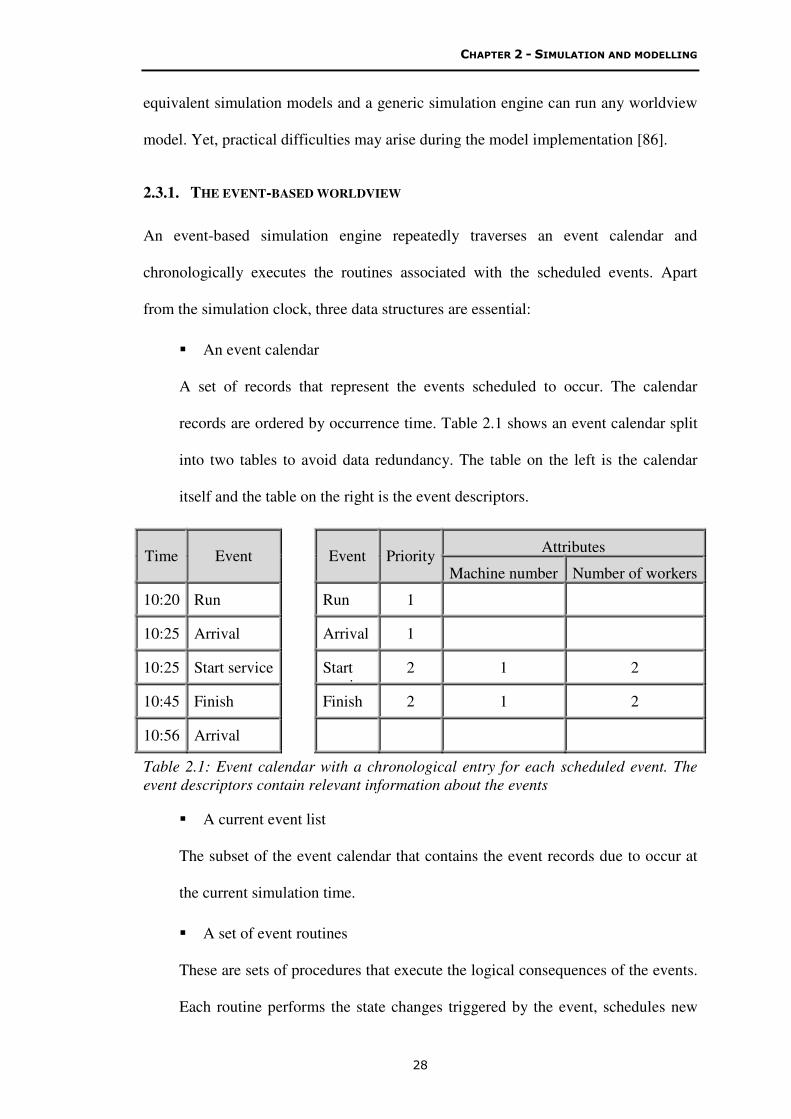
� An event calendar
A set of records that represent the events scheduled to occur. The calendar
records are ordered by occurrence time. Table 2.1 shows an event calendar split
into two tables to avoid data redundancy. The table on the left is the calendar
itself and the table on the right is the event descriptors.
Time Event
Event Priority Attributes
Machine number Number of workers
10:20 Run Run 1
10:25 Arrival Arrival 1
10:25 Start service Start
service
2 1 2
10:45 Finish Finish 2 1 2
10:56 Arrival
Table 2.1: Event calendar with a chronological entry for each scheduled event. The
event descriptors contain relevant information about the events
� A current event list
The subset of the event calendar that contains the event records due to occur at
the current simulation time.
� A set of event routines
These are sets of procedures that execute the logical consequences of the events.
Each routine performs the state changes triggered by the event, schedules new

CHAPTER 2 - SIMULATION AND MODELLING
29
events and deletes the corresponding entry from the current event list [18].
Using a C#-based pseudo-code, the event-based worldview can be expressed by
the following algorithm:
Algorithm event-based simulation()
Description: This algorithm invokes the main components of an
event-based simulation engine.
{
While simulation is not over
{Find the time of the next event;// Traverse the calendar
Update the simulation clock to that time;
Copy to the current event list all the calendar records
whose events are due to occur at this simulation time;
While (current event list != Empty)
{Extract an event record;
Execute the corresponding event routine;}}
}
The logic of an event-based simulation engine is straightforward for small models
as the events are separately handled by the corresponding event routine. Yet, this is an
obstacle to scale up the problem by addition of events as each new event changes the
logical consequences of preceding events and thus the corresponding routines have to
be modified.
2.3.2. THE ACTIVITY-SCANNING WORLDVIEW
An activity-based simulation engine repeatedly scans all activities of the model to
check which are due at the current simulation time. Activity-routines perform the
actions that compose each activity. Using a C#-based pseudo-code, the activity-based
worldview can be expressed by the following algorithm:
Algorithm activity-based simulation()
Description: This algorithm invokes the main components of an
activity-based simulation engine.
{

CHAPTER 2 - SIMULATION AND MODELLING
30
while simulation is not over
{//Traverse the calendar or entities’list
Move the simulation clock to the next event time;
For each activity of the model
{//Check if the activity is due now
if (the activity start time = simulation clock)
//Check if the activity can be performed now
if (the activity conditions hold )
//Perform the activities’actions
{Actions }}}
An activity-based simulation engine is very simple as, besides the simulation
clock, it only requires a list of entities or a calendar and sets of activities routines. The
routines are structured into two phases, a test-head followed by the execution of the
actions which the activity triggers off. However, it is inefficient as, at each simulation
time, it checks all the future activities even though it is known that some are scheduled
for later.
2.3.3. THE PROCESS-BASED WORLDVIEW
A process-based simulation engine is structured into process routines, i.e. sets of
procedures that lead each entity through all the operations it has to pass through from
its arrival at the system to its exit [110]. There can be a process routine for each class
of entities, for example a customer process or a staff process, in which all the
members of the same class are subject to the same activities.
The communication among processes transits the system from one state to the
next. The inter-process communication is coordinated by a process server and the
corresponding process-server routine. The server schedules the execution of the other
processes, alternating indefinitely between starting-service and ending-service, i.e.
switching from busy to idle.
All the processes, while executing, transit from the active state to the passive or

CHAPTER 2 - SIMULATION AND MODELLING
31
the suspend state as illustrated in Fig. 2.10. The arrival of a new entity generates a
new instance of the process. If the server is busy, the new process moves to a passive
state. When the server becomes idle, it schedules a process to be active, transfers the
execution control to it and suspends itself until this entity also suspends itself or
becomes passive. The process server is passive only if there are no processes to
schedule.
Fig. 2.10: State transitions of an entity’s process (left) and of a process server (right)
The communication of processes is comparable to a multitasking or a
multithreading computer operating system [37]. The process server, like the processor,
dispatches the entities’ processes by selecting the process to be active and transferring
the control of the execution to it. The process server becomes passive if there is no
process to dispatch. It also has, like a computer operating system, to perform the
context switching by saving the status of the process that stops running and restoring
the status of the process that runs next.
2.3.4. THE THREE-PHASE WORLDVIEW
The three-phase paradigm for simulation engines classifies the operations to be
simulated into two categories, B and C. B-activities are bound or book-kept to run at a
predictable time. Their duration is deterministic or stochastic, e.g. the duration of
CHAPTER 2 - SIMULATION AND MODELLING
32
setting up a machine, but they will definitely occur when the duration time elapses. C
activities are conditionally run depending on the availability of the entities or
resources with which they cooperate. They cannot be directly scheduled as they
depend on other activities, e.g. assembling a product depends on the availability of
parts to assemble and the status of the assembling machine.
The three-phase simulation algorithm starts by determining the time of the next
event and updating the simulation time accordingly at phase A, runs the B activities
scheduled for this time at phase B and then attempts to run the C activities at phase C.
Using C#-based pseudo-code, the three-phase approach could be expressed
algorithmically as follows:
Algorithm Three-phase-simulation()
Description: This algorithm implements a three-phase simulation
by iteratively invoking each phase procedures.
{
//Reading in the simulation model
Read the Application logic;
//Initialising the simulation clock, the system status, etc.
Initialisation;
While (simulation is not over)
{//Updating the simulation time to the next event occurrence time
APhase;
//Running the B activities scheduled for this simulation time
BPhase;
//Processing the C activities whose head conditions hold
CPhase;
}
//Outputting the results of the simulation
Finalisation;}
The three-phase simulation worldview may be seen as a combination of the
activity-based and event-based worldviews. B activities are processed as if they were
event routines that are executed when the simulation time reaches their scheduling

CHAPTER 2 - SIMULATION AND MODELLING
33
time and C activities are processed by a two-phase routine. This combination results in
an efficiency improvement as, at each simulation time, it does not attempt to run all
the activities as some are known to have been scheduled for later. Also, although B
activities are dealt as if they were events, there is no need to go through all their
possible consequences, which results in an improvement over the event-based
simulation.
The three phase simulation approach presents important characteristics such as
high modularity and extensibility by addition of B and C activities. However, it is
rather more complex to understand and implement than the event-based and the
activity based simulation.
2.4. THE CHAPTER IN CONTEXT
In this chapter, relevant concepts from modelling and simulation fields are reviewed
to clarify how simulation acts and interacts with modelling to analyse complex
systems. The simulation of complex systems is dissected and the underlying concepts
are explained, focussing on DES systems. The application logic and the simulation
engine which executes it through time are revisited. This calls for the definition of the
time flow mechanisms, the ‘classical’ simulation worldviews and the simulation
engine which they mirror.
The size and the complexity of DE simulations reveal the importance of computer
simulation in repeatedly emulating their operation over a period of time. This calls for
the revision of concepts from computing that permit us to understand the co-evolution
of simulation and computer science and to make sense of current trends in simulation
software so as to devise a path towards future developments. Computing and
simulation concepts are reviewed in the next chapter.
![Gillimberg Farm, Part I: A Pilot Struggles to Take · PDF file2.1 StateLand 2.1.1 500,000ha+[thiswaspresumablyintended tobe50,000ha]6 2.1.2 LebowaDevelopmentCorporation 2.1.3 Statefarming](https://img.pdfslide.us/doc/110x75/5ab889207f8b9aa6018cc579/gillimberg-farm-part-i-a-pilot-struggles-to-take-stateland-211-500000hathiswaspresumablyintended.jpg)