Embed Size (px)
Citation preview
WWW.MINITAB.COM
MINITAB ASSISTANT WHITE PAPER
This paper explains the research conducted by Minitab statisticians to develop the methods and
data checks used in the Assistant in Minitab Statistical Software.
2-Sample t-Test
Overview A 2-sample t-test can be used to compare whether two independent groups differ. This test is
derived under the assumptions that both populations are normally distributed and have equal
variances. Although the assumption of normality is not critical (Pearson, 1931; Barlett, 1935;
Geary, 1947), the assumption of equal variances is critical if the sample sizes are markedly
different (Welch, 1937; Horsnell, 1953).
Some practitioners first perform a preliminary test to evaluate equal variances before they
perform the classical 2-sample t procedure. This approach has serious drawbacks, however,
because these variance tests are subject to important assumptions and limitations. For example,
many tests for equal variances, such as the classical F-test, are sensitive to departures from
normality. Other tests that do not rely on the assumption of normality, such as Levene/Brown-
Forsythe, have low power to detect a difference between variances.
B.L. Welch developed an approximation method for comparing the means of two independent
normal populations when their variances are not necessarily equal (Welch, 1947). Because
Welch’s modified t-test is not derived under the assumption of equal variances, it allows users to
compare the means of two populations without first having to test for equal variances.
In this paper, we compare Welch’s modified t method with the classical 2-sample t procedure
and determine which procedure is the most reliable. We also describe the following data checks
that are automatically performed and displayed in the Assistant Report Card and explain how
they affect the results of the analysis:
Normality
Unusual data
Sample size
2-SAMPLE t-TEST 2
2-sample t-test method
Classical 2- -test If data come from two normal populations with the same variances, the classical 2-sample t-test
is as powerful or more powerful than Welch’s t-test. The normality assumption is not critical for
the classical procedure (Pearson, 1931; Barlett, 1935; Geary, 1947), but the equal-variance
assumption is important to ensure valid results. More specifically, the classical procedure is
sensitive to the assumption of equal variances when the sample sizes differ regardless of how
large the samples are (Welch, 1937; Horsnell, 1953). In practice, however, the equal variance
assumption rarely holds true, which can lead to higher Type I error rates. Therefore, if the
classical 2-sample t-test is used when two samples have different variances, the test is more
likely to produce incorrect results.
Welch’s t-test is a viable alternative to the classical t-test because it does not assume equal
variances and therefore is insensitive to unequal variances for all sample sizes. However, Welch’s
t-test is approximation-based and its performance in small sample sizes may be questionable.
We wanted to determine whether Welch’s t-test or the classical 2-sample t-test is the most
reliable and practical test to use in the Assistant.
Objective
We wanted to determine, through simulation studies and theoretical derivations, whether
Welch’s t-test or the classical 2-sample t-test is more reliable. More specifically, we want to
examine:
The Type I and Type II error rates of both the classical 2-sample t-test and Welch’s t-test
at various sample sizes when the data are normally distributed and the variances are
equal.
The Type I and Type II error rates of Welch’s t-test for unbalanced and unequal-variance
designs for which the classical 2-sample t-test fails.
Method
Our simulations focused on three areas:
We compared simulated test results of the classical 2-sample t-test and Welch’s t-test
under various model assumptions, including normality, nonnormality, equal variances,
unequal variances, balanced, and unbalanced designs. For more details, see Appendix A.
We derived the power function for Welch’s t-test and compared it with the power
function of the classical 2-sample t-test. For more details, see Appendix B.
We studied the impact of nonnormality on the theoretical power function of Welch’s
t-test.
2-SAMPLE t-TEST 3
Results
When the assumptions for the classical 2-sample t model hold, Welch’s t-test performs as well
or nearly as well as the classical 2-sample t-test except for small unbalanced designs. However,
the classical 2-sample t-test may also perform poorly when designs are small and unbalanced,
due to its sensitivity to the equal variance assumption. Moreover, in practical settings, it is
difficult to establish that two populations have exactly the same variance. Therefore, the
theoretical superiority of the classical 2-sample test over Welch’s t-test has a little or no practical
value. For this reason, the Assistant uses Welch’s t-test to compare the means of two
populations. For the detailed simulation results, see Appendices A, B, and C.
2-SAMPLE t-TEST 4
Data checks
Normality Welch’s t-test, the method used in the Assistant to compare the means of two independent
populations, is derived under the assumption that the populations are normally distributed.
Fortunately, even when data are not normally distributed, Welch’s t-test works well if the
samples are large enough.
Objective
We wanted to determine how closely the simulated levels of significance for the Welch method
and the classical 2-sample t-test matched the target level of significance (Type I error rate) of
0.05.
Method
We performed simulations of Welch’s t-test and the classical 2-sample t-test on 10,000 pairs of
independent samples generated from normal, skewed, and contaminated normal (equal and
unequal variances) populations. The samples were of various sizes. The normal population
serves as a control population for comparison purposes. For each condition, we calculated the
simulated significance levels and compared them with the target, or nominal, significance level
of 0.05. If the test performs well, the simulated significance levels should be close to 0.05.
Results
For moderate or large samples, Welch’s t-test maintains its Type I error rates for normal as well
as nonnormal data. The simulated significance levels are close to the targeted significance level
when both sample sizes are at least 15. See Appendix A for more details.
Because the test performs well with relatively small samples, the Assistant does not test the data
for normality. Instead, it checks the size of the samples and displays the following status
indicators in the Report Card:
Status Condition
Both sample sizes are at least 15; normality is not an issue.
At least one of the sample sizes < 15; normality may be an issue.
2-SAMPLE t-TEST 5
Unusual data Unusual data are extremely large or small data values, also known as outliers. Unusual data can
have a strong influence on the results of the analysis. When the sample is small, they can affect
the chances of finding statistically significant results. Unusual data can indicate problems with
data collection or unusual behavior of a process. Therefore, these data points are often worth
investigating and should be corrected when possible.
Objective
We wanted to develop a method to check for data values that are very large or very small
relative to the overall sample and that may affect the results of the analysis
Method
We developed a method to check for unusual data based on the method described by Hoaglin,
Iglewicz, and Tukey (1986) to identify outliers in boxplots.
Results
The Assistant identifies a data point as unusual if it is more than 1.5 times the interquartile range
beyond the lower or upper quartile of the distribution. The lower and upper quartiles are the
25th and 75th percentiles of the data. The interquartile range is the difference between the two
quartiles. This method works well even when there are multiple outliers because it makes it
possible to detect each specific outlier.
Outliers tend to have an influence on the power function only when the sample sizes are very
small. In general, when outliers are present the observed power values tend to be a bit higher
than the targeted theoretical power values. This pattern can be seen in Figure 10 in Appendix C
where the simulated and theoretical power curves are not reasonably close until the minimum
sample size reaches 15.
When checking for unusual data, the Assistant Report Card for the 2-sample t-test displays the
following status indicators:
Status Condition
There are no unusual data points.
At least one data point is unusual and may affect the test results.
2-SAMPLE t-TEST 6
Sample size Typically, a hypothesis test is performed to gather evidence to reject the null hypothesis of “no
difference”. If the samples are too small, the power of the test may not be adequate to detect a
difference between the means when one actually exists, which results in a Type II error. It is
therefore crucial to ensure that the sample sizes are sufficiently large to detect practically
important differences with high probability.
Objective
If the current data does not provide sufficient evidence against the null hypothesis, we want to
determine if the sample sizes are large enough for the test to detect practical differences of
interest with high probability. Although the objective of sample size planning is to ensure that
the samples are large enough to detect important differences with high probability, the samples
should not be so large that meaningless differences become statistically significant with high
probability.
Method
The power and sample size analysis is based upon the theoretical power function of the specific
test that is used to perform the statistical analysis. For the Welch t-test, this power function
depends upon the sample sizes, the difference between the two population means, and the true
variances of the two populations. For more details, see Appendix B.
Results
When the data does not provide enough evidence against the null hypothesis, the Assistant
calculates practical differences that can be detected with an 80% and a 90% probability for the
given sample sizes. In addition, if the user provides a practical difference of interest, the
Assistant calculates the sample sizes that yield an 80% and a 90% chance of detecting the
difference.
There is no general result to report because the results depend on the user’s specific samples.
However, you can refer to Appendices B and C for more information about Welch’s test power
function.
When checking for power and sample size, the Assistant Report Card for the 2-sample t-test
displays the following status indicators:
Status Condition
The test finds a difference between the means, so power is not an issue.
OR
Power is sufficient. The test did not find a difference between the means, but the sample is large enough to provide at least a 90% chance of detecting the given difference.
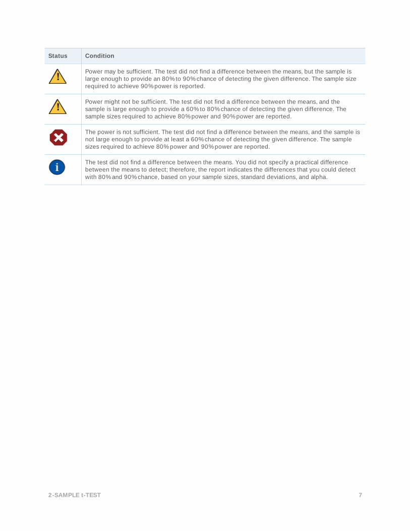
2-SAMPLE t-TEST 7
Status Condition
Power may be sufficient. The test did not find a difference between the means, but the sample is large enough to provide an 80% to 90% chance of detecting the given difference. The sample size required to achieve 90% power is reported.
Power might not be sufficient. The test did not find a difference between the means, and the sample is large enough to provide a 60% to 80% chance of detecting the given difference. The sample sizes required to achieve 80% power and 90% power are reported.
The power is not sufficient. The test did not find a difference between the means, and the sample is not large enough to provide at least a 60% chance of detecting the given difference. The sample sizes required to achieve 80% power and 90% power are reported.
The test did not find a difference between the means. You did not specify a practical difference between the means to detect; therefore, the report indicates the differences that you could detect with 80% and 90% chance, based on your sample sizes, standard deviations, and alpha.
2-SAMPLE t-TEST 8
References Arnold, S. F. (1990). Mathematical Statistics. Englewood Cliffs, NJ: Prentice-Hall, Inc.
Aspin, A. A. (1949). Tables for Use in Comparisons whose Accuracy Involves Two Variances,
Separately Estimated, Biometrika, 36, 290-296.
Bartlett, M. S. (1935). The effect of non-normality on the t-distribution. Proceedings of the
Cambridge Philosophical Society, 31, 223-231.
Box, G. E. P. (1953). Non-normality and Tests on Variances, Biometrika, 40, 318-335.
Geary, R. C. (1947). Testing for Normality, Biometrika, 34, 209-242.
Hoaglin, D. C., Iglewicz, B., and Tukey, J. W. (1986). Performance of Some Resistant Rules for
Outlier Labeling. Journal of the American Statistical Association, 81, 991-999.
Horsnell, G. (1953). The effect of unequal group variances on the F test for homogeneity of
group means. Biometrika, 40, 128-136.
James, G. S. (1951). The comparison of several groups of observations when the ratios of the
populations variances are unknown, Biometrika, 38, 324-329.
Kulinskaya, E. Staudte, R. G. and Gao, H. (2003). Power Approximations in Testing for unequal
Means in a One-Way Anova Weighted for Unequal Variances, Communication in Statistics,
32(12), 2353-2371.
Lehmann, E. L. (1959). Testing statistical hypotheses. New York, NY: Wiley.
Neyman, J., Iwaszkiewicz, K. & Kolodziejczyk, S. (1935). Statistical problems in agricultural
experimentation, Journal of the Royal Statistical Society, Series B, 2, 107-180.
Pearson, E. S. (1931). The Analysis of variance in case of non-normal variation, Biometrika, 23,
114-133.
Pearson, E.S. & Hartley, H.O. (Eds.). (1954). Biometrika Tables for Statisticians, Vol. I. London:
Cambridge University Press.
Srivastava, A. B. L. (1958). Effect of non-normality on the power function of t-test, Biometrika, 45,
421-429.
Welch, B. L. (1951). On the comparison of several mean values: an alternative approach.
Biometrika, 38, 330-336.
Welch, B. L. (1947). The generalization of “Student’s” problem when several different population
variances are involved. Biometrika, 34, 28-35.
Welch, B. L. (1938). The significance of the difference between two means when the population
variances are unequal, Biometrika, 29, 350-362.
Wolfram, S. (1999). The Mathematica Book (4th ed.). Champaign, IL: Wolfram Media/Cambridge
University Press.
2-SAMPLE t-TEST 9
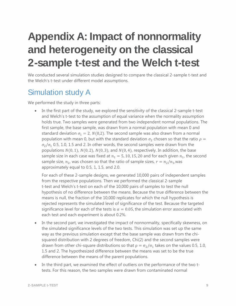
Appendix A: Impact of nonnormality and heterogeneity on the classical 2-sample t-test and the Welch t-test We conducted several simulation studies designed to compare the classical 2-sample t-test and
the Welch’s t-test under different model assumptions.
Simulation study A We performed the study in three parts:
In the first part of the study, we explored the sensitivity of the classical 2-sample t-test
and Welch’s t-test to the assumption of equal variance when the normality assumption
holds true. Two samples were generated from two independent normal populations. The
first sample, the base sample, was drawn from a normal population with mean 0 and
standard deviation 𝜎1 = 2, 𝑁(0,2). The second sample was also drawn from a normal
population with mean 0, but with the standard deviation 𝜎2 chosen so that the ratio 𝜌 =
𝜎2/𝜎1 0.5, 1.0, 1.5 and 2. In other words, the second samples were drawn from the
populations 𝑁(0, 1), 𝑁(0, 2), 𝑁(0, 3), and 𝑁(0, 4), respectively. In addition, the base
sample size in each case was fixed at 𝑛1 = 5, 10, 15, 20 and for each given 𝑛1, the second
sample size, 𝑛2, was chosen so that the ratio of sample sizes, 𝑟 = 𝑛2/𝑛1,was
approximately equal to 0.5, 1, 1.5, and 2.0.
For each of these 2-sample designs, we generated 10,000 pairs of independent samples
from the respective populations. Then we performed the classical 2-sample
t-test and Welch’s t-test on each of the 10,000 pairs of samples to test the null
hypothesis of no difference between the means. Because the true difference between the
means is null, the fraction of the 10,000 replicates for which the null hypothesis is
rejected represents the simulated level of significance of the test. Because the targeted
significance level for each of the tests is 𝛼 = 0.05, the simulation error associated with
each test and each experiment is about 0.2%.
In the second part, we investigated the impact of nonnormality, specifically skewness, on
the simulated significance levels of the two tests. This simulation was set up the same
way as the previous simulation except that the base sample was drawn from the chi-
squared distribution with 2 degrees of freedom, Chi(2) and the second samples were
drawn from other chi-square distributions so that ρ = σ2/σ1 takes on the values 0.5, 1.0,
1.5 and 2. The hypothesized difference between the means was set to be the true
difference between the means of the parent populations.
In the third part, we examined the effect of outliers on the performance of the two t-
tests. For this reason, the two samples were drawn from contaminated normal
2-SAMPLE t-TEST 10
distributions. A contaminated normal population CN(p, σ) is a mixture of two normal
populations: the N(0,1) population and the normal N(0, σ) population. We define a
contaminated normal distribution as:
𝐶𝑁(𝑝, 𝜎) = 𝑝𝑁(0,1) + (1 − 𝑝)𝑁(0, 𝜎)
where p is the mixing parameter and 1 − p is the proportion of contamination or proportion of
outliers. It is easy to show that if X is distributed as 𝐶𝑁(𝑝, 𝜎) then its mean is 𝜇𝑋 = 0 and its
standard deviation is 𝜎𝑋 = √𝑝 + (1 − 𝑝)𝜎2.
The base sample was drawn from 𝐶𝑁(. 8, 4) and the second sample was drawn from the
contaminated normal 𝐶𝑁(. 8, 𝜎). The parameter 𝜎 was chosen so that the ratio of the standard
deviations of the two (contaminated) populations 𝜌 = 𝜎2/𝜎1 equals 0.5, 1.0, 1.5 and 2, just like in
parts I and II. Because 𝜎1 = √. 8 + (1 − .8) ∗ 16 = 2.0, this results in choosing 𝜎 = 1, 4, 6.40, 8.72,
respectively. In other words, the second samples were drawn from 𝐶𝑁(. 8, 1), 𝐶𝑁(. 8, 4),
𝐶𝑁(. 8, 6.4), and 𝐶𝑁(. 8, 8.72). We then performed the simulations as described in Part I.
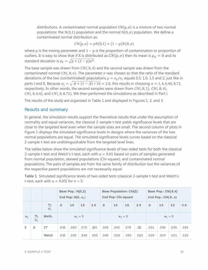
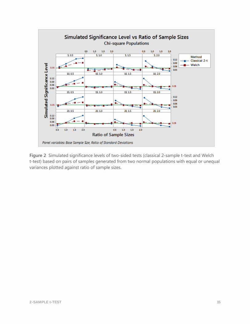
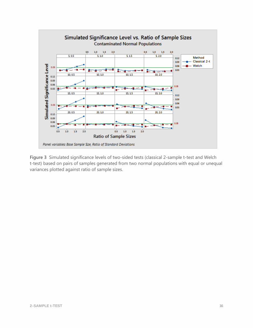
The results of the study are organized in Table 1 and displayed in Figures 1, 2, and 3.
Results and summary
In general, the simulation results support the theoretical results that under the assumption of
normality and equal variances, the classical 2-sample t-test yields significance levels that are
close to the targeted level even when the sample sizes are small. The second column of plots in
Figure 1 displays the simulated significance levels in designs where the variances of the two
normal populations are equal. The simulated significance levels curves based on the classical
2-sample t-test are undistinguishable from the targeted level lines.
The tables below show the simulated significance levels of two-sided tests for both the classical
2-sample t-test and Welch’s t-test, each with α = 0.05 based on pairs of samples generated
from normal population, skewed populations (Chi-square), and contaminated normal
populations. The pairs of samples are from the same family of distribution but the variances of
the respective parent populations are not necessarily equal.
Table 1 Simulated significance levels of two-sided tests (classical 2-sample t-test and Welch’s
t-test, each with α = 0.05) for n = 5.
Base Pop.: N(0,2)
2nd Pop: N(0, 𝝈𝟐)
Base Population: Chi(2)
2nd Pop: Chi-square
Base Pop.: CN(.8,4)
2nd Pop.: CN(.8, 𝝈)
𝝈𝟐
𝝈𝟏 .5 1.0 1.5 2.0 .5 1.0 1.5 2.0 .5 1.0 1.5 2.0
𝒏𝟐 𝒏𝟐
𝒏𝟏 Meth. 𝒏𝟏 = 𝟓 𝒏𝟏 = 𝟓 𝒏𝟏 = 𝟓
3 .6 2T .035 .050 .079 .105 .058 .042 .078 .113 .031 .036 .035 .034
Welch .035 .039 .049 .055 .048 .029 .055 .063 .029 .024 .021 .020
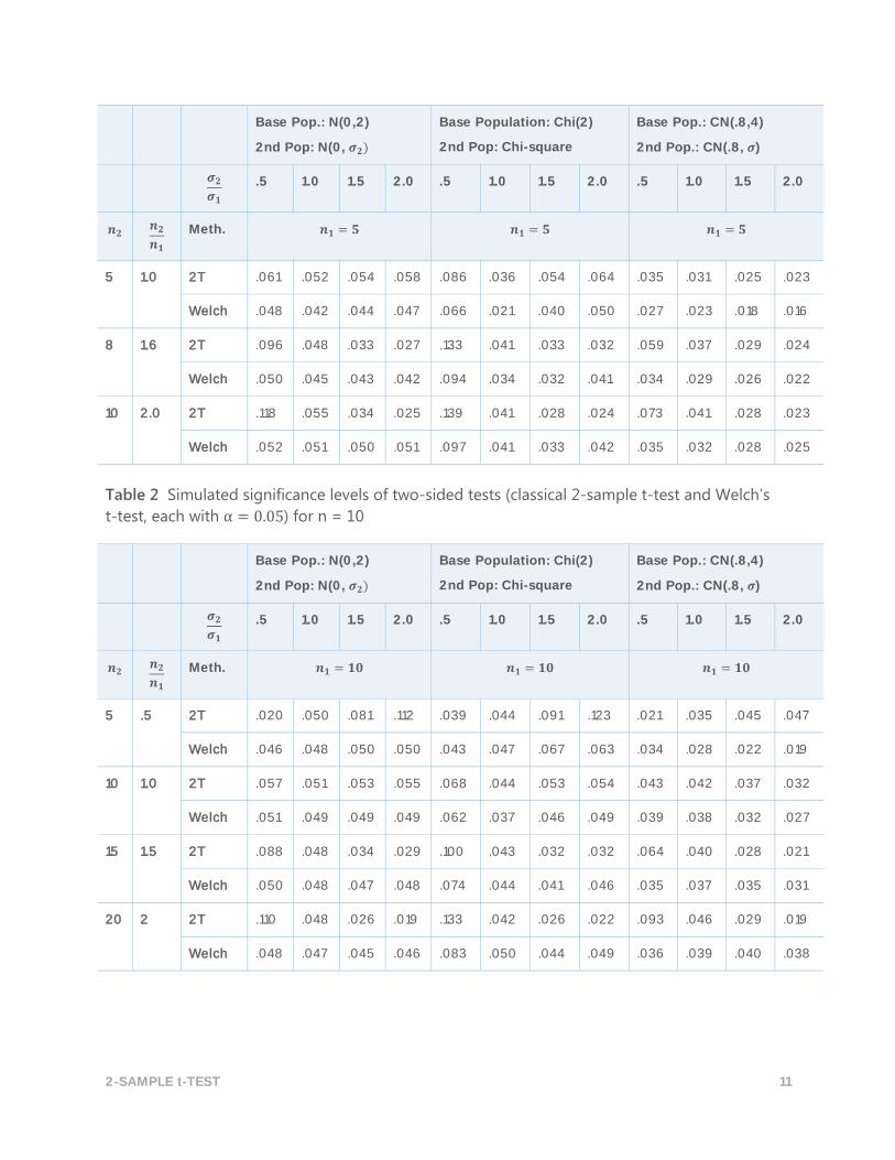
2-SAMPLE t-TEST 11
Base Pop.: N(0,2)
2nd Pop: N(0, 𝝈𝟐)
Base Population: Chi(2)
2nd Pop: Chi-square
Base Pop.: CN(.8,4)
2nd Pop.: CN(.8, 𝝈)
𝝈𝟐
𝝈𝟏 .5 1.0 1.5 2.0 .5 1.0 1.5 2.0 .5 1.0 1.5 2.0
𝒏𝟐 𝒏𝟐
𝒏𝟏 Meth. 𝒏𝟏 = 𝟓 𝒏𝟏 = 𝟓 𝒏𝟏 = 𝟓
5 1.0 2T .061 .052 .054 .058 .086 .036 .054 .064 .035 .031 .025 .023
Welch .048 .042 .044 .047 .066 .021 .040 .050 .027 .023 .018 .016
8 1.6 2T .096 .048 .033 .027 .133 .041 .033 .032 .059 .037 .029 .024
Welch .050 .045 .043 .042 .094 .034 .032 .041 .034 .029 .026 .022
10 2.0 2T .118 .055 .034 .025 .139 .041 .028 .024 .073 .041 .028 .023
Welch .052 .051 .050 .051 .097 .041 .033 .042 .035 .032 .028 .025
Table 2 Simulated significance levels of two-sided tests (classical 2-sample t-test and Welch’s
t-test, each with α = 0.05) for n = 10
Base Pop.: N(0,2)
2nd Pop: N(0, 𝝈𝟐)
Base Population: Chi(2)
2nd Pop: Chi-square
Base Pop.: CN(.8,4)
2nd Pop.: CN(.8, 𝝈)
𝝈𝟐
𝝈𝟏 .5 1.0 1.5 2.0 .5 1.0 1.5 2.0 .5 1.0 1.5 2.0
𝒏𝟐 𝒏𝟐
𝒏𝟏 Meth. 𝒏𝟏 = 𝟏𝟎 𝒏𝟏 = 𝟏𝟎 𝒏𝟏 = 𝟏𝟎
5 .5 2T .020 .050 .081 .112 .039 .044 .091 .123 .021 .035 .045 .047
Welch .046 .048 .050 .050 .043 .047 .067 .063 .034 .028 .022 .019
10 1.0 2T .057 .051 .053 .055 .068 .044 .053 .054 .043 .042 .037 .032
Welch .051 .049 .049 .049 .062 .037 .046 .049 .039 .038 .032 .027
15 1.5 2T .088 .048 .034 .029 .100 .043 .032 .032 .064 .040 .028 .021
Welch .050 .048 .047 .048 .074 .044 .041 .046 .035 .037 .035 .031
20 2 2T .110 .048 .026 .019 .133 .042 .026 .022 .093 .046 .029 .019
Welch .048 .047 .045 .046 .083 .050 .044 .049 .036 .039 .040 .038
2-SAMPLE t-TEST 12
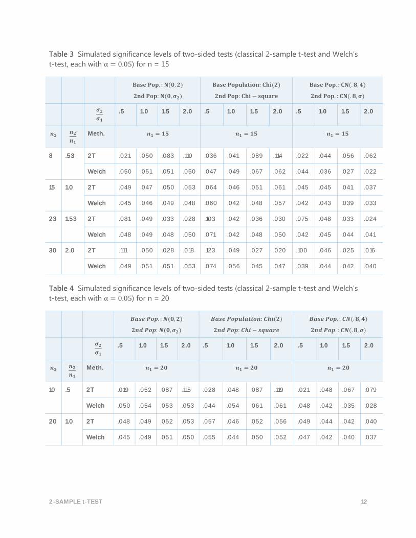
Table 3 Simulated significance levels of two-sided tests (classical 2-sample t-test and Welch’s
t-test, each with α = 0.05) for n = 15
𝐁𝐚𝐬𝐞 𝐏𝐨𝐩. : 𝐍(𝟎, 𝟐)
𝟐𝐧𝐝 𝐏𝐨𝐩: 𝐍(𝟎, 𝛔𝟐)
𝐁𝐚𝐬𝐞 𝐏𝐨𝐩𝐮𝐥𝐚𝐭𝐢𝐨𝐧: 𝐂𝐡𝐢(𝟐)
𝟐𝐧𝐝 𝐏𝐨𝐩: 𝐂𝐡𝐢 − 𝐬𝐪𝐮𝐚𝐫𝐞
𝐁𝐚𝐬𝐞 𝐏𝐨𝐩. : 𝐂𝐍(. 𝟖, 𝟒)
𝟐𝐧𝐝 𝐏𝐨𝐩. : 𝐂𝐍(. 𝟖, 𝛔)
𝝈𝟐
𝝈𝟏 .5 1.0 1.5 2.0 .5 1.0 1.5 2.0 .5 1.0 1.5 2.0
𝒏𝟐 𝒏𝟐
𝒏𝟏 Meth. 𝒏𝟏 = 𝟏𝟓 𝒏𝟏 = 𝟏𝟓 𝒏𝟏 = 𝟏𝟓
8 .53 2T .021 .050 .083 .110 .036 .041 .089 .114 .022 .044 .056 .062
Welch .050 .051 .051 .050 .047 .049 .067 .062 .044 .036 .027 .022
15 1.0 2T .049 .047 .050 .053 .064 .046 .051 .061 .045 .045 .041 .037
Welch .045 .046 .049 .048 .060 .042 .048 .057 .042 .043 .039 .033
23 1.53 2T .081 .049 .033 .028 .103 .042 .036 .030 .075 .048 .033 .024
Welch .048 .049 .048 .050 .071 .042 .048 .050 .042 .045 .044 .041
30 2.0 2T .111 .050 .028 .018 .123 .049 .027 .020 .100 .046 .025 .016
Welch .049 .051 .051 .053 .074 .056 .045 .047 .039 .044 .042 .040
Table 4 Simulated significance levels of two-sided tests (classical 2-sample t-test and Welch’s
t-test, each with α = 0.05) for n = 20
𝑩𝒂𝒔𝒆 𝑷𝒐𝒑. : 𝑵(𝟎, 𝟐)
𝟐𝒏𝒅 𝑷𝒐𝒑: 𝑵(𝟎, 𝝈𝟐)
𝑩𝒂𝒔𝒆 𝑷𝒐𝒑𝒖𝒍𝒂𝒕𝒊𝒐𝒏: 𝑪𝒉𝒊(𝟐)
𝟐𝒏𝒅 𝑷𝒐𝒑: 𝑪𝒉𝒊 − 𝒔𝒒𝒖𝒂𝒓𝒆
𝑩𝒂𝒔𝒆 𝑷𝒐𝒑. : 𝑪𝑵(. 𝟖, 𝟒)
𝟐𝒏𝒅 𝑷𝒐𝒑. : 𝑪𝑵(. 𝟖, 𝝈)
𝝈𝟐
𝝈𝟏 .5 1.0 1.5 2.0 .5 1.0 1.5 2.0 .5 1.0 1.5 2.0
𝒏𝟐 𝒏𝟐
𝒏𝟏 Meth. 𝒏𝟏 = 𝟐𝟎 𝒏𝟏 = 𝟐𝟎 𝒏𝟏 = 𝟐𝟎
10 .5 2T .019 .052 .087 .115 .028 .048 .087 .119 .021 .048 .067 .079
Welch .050 .054 .053 .053 .044 .054 .061 .061 .048 .042 .035 .028
20 1.0 2T .048 .049 .052 .053 .057 .046 .052 .056 .049 .044 .042 .040
Welch .045 .049 .051 .050 .055 .044 .050 .052 .047 .042 .040 .037
2-SAMPLE t-TEST 13
𝑩𝒂𝒔𝒆 𝑷𝒐𝒑. : 𝑵(𝟎, 𝟐)
𝟐𝒏𝒅 𝑷𝒐𝒑: 𝑵(𝟎, 𝝈𝟐)
𝑩𝒂𝒔𝒆 𝑷𝒐𝒑𝒖𝒍𝒂𝒕𝒊𝒐𝒏: 𝑪𝒉𝒊(𝟐)
𝟐𝒏𝒅 𝑷𝒐𝒑: 𝑪𝒉𝒊 − 𝒔𝒒𝒖𝒂𝒓𝒆
𝑩𝒂𝒔𝒆 𝑷𝒐𝒑. : 𝑪𝑵(. 𝟖, 𝟒)
𝟐𝒏𝒅 𝑷𝒐𝒑. : 𝑪𝑵(. 𝟖, 𝝈)
𝝈𝟐
𝝈𝟏 .5 1.0 1.5 2.0 .5 1.0 1.5 2.0 .5 1.0 1.5 2.0
𝒏𝟐 𝒏𝟐
𝒏𝟏 Meth. 𝒏𝟏 = 𝟐𝟎 𝒏𝟏 = 𝟐𝟎 𝒏𝟏 = 𝟐𝟎
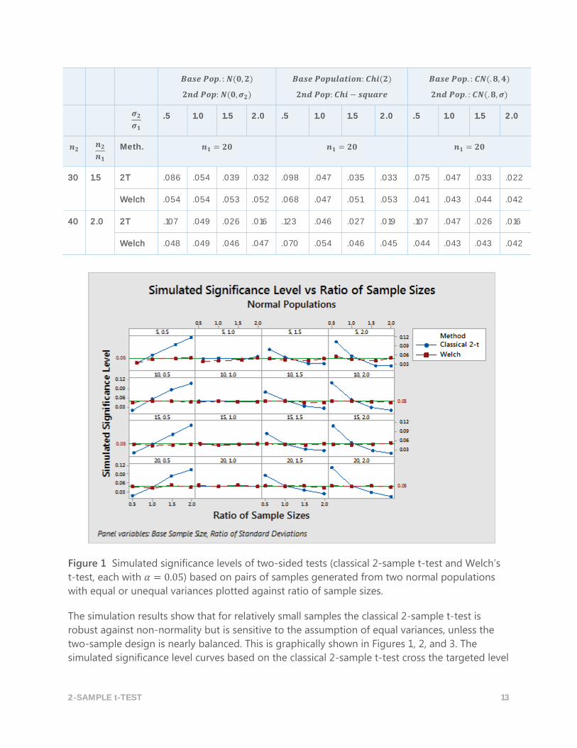
30 1.5 2T .086 .054 .039 .032 .098 .047 .035 .033 .075 .047 .033 .022
Welch .054 .054 .053 .052 .068 .047 .051 .053 .041 .043 .044 .042
40 2.0 2T .107 .049 .026 .016 .123 .046 .027 .019 .107 .047 .026 .016
Welch .048 .049 .046 .047 .070 .054 .046 .045 .044 .043 .043 .042
Figure 1 Simulated significance levels of two-sided tests (classical 2-sample t-test and Welch’s
t-test, each with 𝛼 = 0.05) based on pairs of samples generated from two normal populations
with equal or unequal variances plotted against ratio of sample sizes.
The simulation results show that for relatively small samples the classical 2-sample t-test is
robust against non-normality but is sensitive to the assumption of equal variances, unless the
two-sample design is nearly balanced. This is graphically shown in Figures 1, 2, and 3. The
simulated significance level curves based on the classical 2-sample t-test cross the targeted level
2-SAMPLE t-TEST 14
line at the point where the ratio of sample sizes is 1.0, even when the variances are very
different. For all three families of distributions (normal, chi-square, and contaminated normal
populations), if the sample sizes are different, the simulated significance levels of the classical
2-sample t-test are near the targeted level only when the variances are equal. This is depicted
on the second column of plots in each of the figures 1, 2, and 3.
The performance of the classical t-test is undesirable when the design is unbalanced and the
variances are unequal. Even small disparities between the variances are troublesome. For those
unequal-variance, unbalanced designs, normality of the data does not improve the simulated
significance levels. In fact, the simulated significance levels fall away from the targeted level as
the sample sizes increase regardless of the parent population. When the larger sample is drawn
from the population with larger variance, the simulated significance levels are smaller than the
targeted level. When the larger samples are drawn from the population with smaller variance,
the simulated levels are larger than the targeted levels. Arnold (1990, page 372) makes a similar
remark when examining the asymptotic distribution of the classical 2-sample t-test statistic
under the unequal-variance assumption.
The Welch 2-sample t-test, on the other hand, is impervious to departures from the equal-
variance assumption, as illustrated in Figures 1, 2, and 3. This is not surprising since the Welch
t-test is not derived under the assumption of equal variances. The normal assumption from
which Welch’s t-test is derived appears to be important only when the minimum of the two
samples sizes is very small. For larger samples, however, the test becomes immune to departures
from the normality assumption. This is illustrated in Figures 2 and 3 where the simulated
significance levels remain consistently close to the targeted level when the minimum size of the
two samples is 15. When both samples are generated from the chi-square distribution with 2
degrees of freedom and the size of both samples is 15, the simulated significance level is 0.042
(see Table 3).
Outliers also do not appear to affect the performance of Welch’s t-test when the minimum size
of the two samples is large enough. Table 3 and Figure 3 show that when the minimum size of
the two samples is at least 15, then the simulated significance levels are near the targeted level
(the simulated significance levels are 0.045, 0.045, 0.041, 0.037 when the ratio of standard
deviations are 0.5, 1.0, 1.5 and 2.0 respectively).
These results show that for most practical purposes, the Welch 2-sample t-test performs better
than the classical 2-sample t-test in terms of its simulated significance levels or Type I error rate.
2-SAMPLE t-TEST 15
Figure 2 Simulated significance levels of two-sided tests (classical 2-sample t-test and Welch
t-test) based on pairs of samples generated from two normal populations with equal or unequal
variances plotted against ratio of sample sizes.
2-SAMPLE t-TEST 16
Figure 3 Simulated significance levels of two-sided tests (classical 2-sample t-test and Welch
t-test) based on pairs of samples generated from two normal populations with equal or unequal
variances plotted against ratio of sample sizes.
2-SAMPLE t-TEST 17
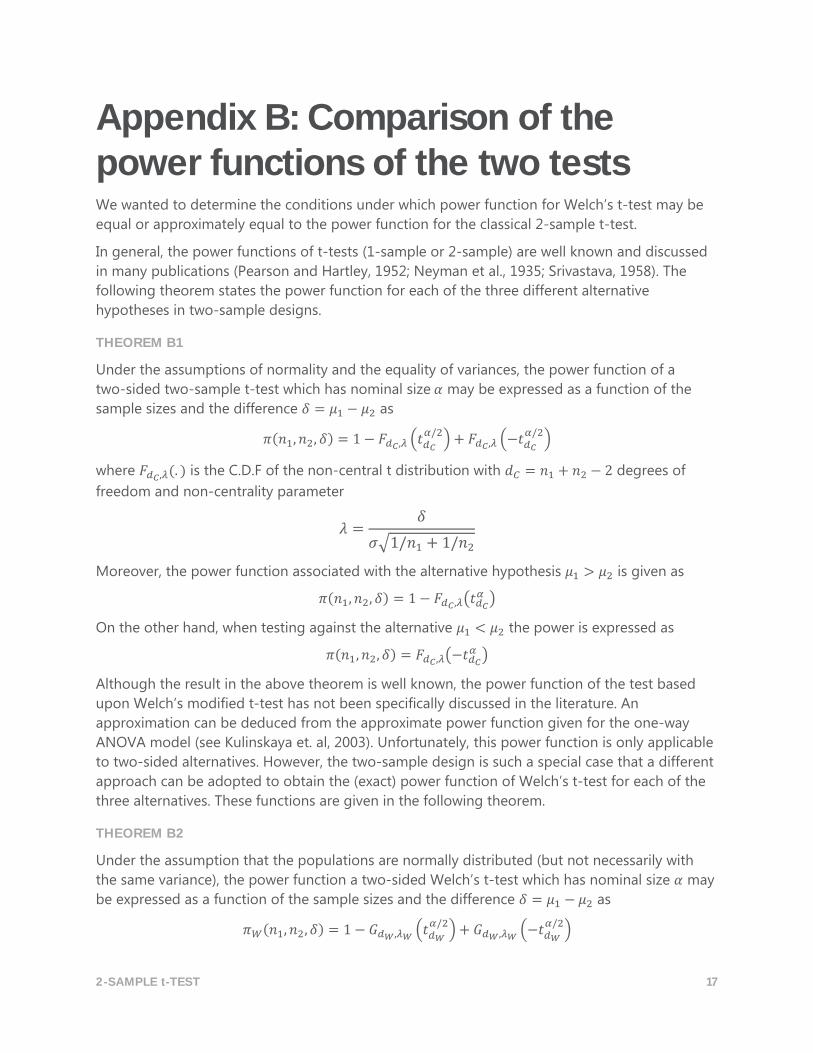
Appendix B: Comparison of the power functions of the two tests We wanted to determine the conditions under which power function for Welch’s t-test may be
equal or approximately equal to the power function for the classical 2-sample t-test.
In general, the power functions of t-tests (1-sample or 2-sample) are well known and discussed
in many publications (Pearson and Hartley, 1952; Neyman et al., 1935; Srivastava, 1958). The
following theorem states the power function for each of the three different alternative
hypotheses in two-sample designs.
THEOREM B1
Under the assumptions of normality and the equality of variances, the power function of a
two-sided two-sample t-test which has nominal size 𝛼 may be expressed as a function of the
sample sizes and the difference 𝛿 = 𝜇1 − 𝜇2 as
𝜋(𝑛1, 𝑛2, 𝛿) = 1 − 𝐹𝑑𝐶,𝜆 (𝑡𝑑𝐶
𝛼/2) + 𝐹𝑑𝐶,𝜆 (−𝑡𝑑𝐶
𝛼/2)
where 𝐹𝑑𝐶,𝜆(. ) is the C.D.F of the non-central t distribution with 𝑑𝐶 = 𝑛1 + 𝑛2 − 2 degrees of
freedom and non-centrality parameter
𝜆 =𝛿
𝜎√1/𝑛1 + 1/𝑛2
Moreover, the power function associated with the alternative hypothesis 𝜇1 > 𝜇2 is given as
𝜋(𝑛1, 𝑛2, 𝛿) = 1 − 𝐹𝑑𝐶,𝜆(𝑡𝑑𝐶
𝛼 )
On the other hand, when testing against the alternative 𝜇1 < 𝜇2 the power is expressed as
𝜋(𝑛1, 𝑛2, 𝛿) = 𝐹𝑑𝐶,𝜆(−𝑡𝑑𝐶
𝛼 )
Although the result in the above theorem is well known, the power function of the test based
upon Welch’s modified t-test has not been specifically discussed in the literature. An
approximation can be deduced from the approximate power function given for the one-way
ANOVA model (see Kulinskaya et. al, 2003). Unfortunately, this power function is only applicable
to two-sided alternatives. However, the two-sample design is such a special case that a different
approach can be adopted to obtain the (exact) power function of Welch’s t-test for each of the
three alternatives. These functions are given in the following theorem.
THEOREM B2
Under the assumption that the populations are normally distributed (but not necessarily with
the same variance), the power function a two-sided Welch’s t-test which has nominal size 𝛼 may
be expressed as a function of the sample sizes and the difference 𝛿 = 𝜇1 − 𝜇2 as
𝜋𝑊(𝑛1, 𝑛2, 𝛿) = 1 − 𝐺𝑑𝑊,𝜆𝑊(𝑡𝑑𝑊
𝛼/2) + 𝐺𝑑𝑊,𝜆𝑊
(−𝑡𝑑𝑊
𝛼/2)
2-SAMPLE t-TEST 18
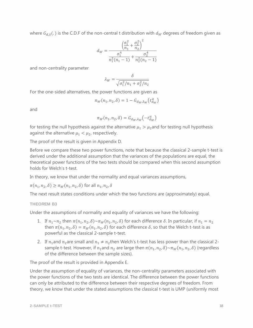
where 𝐺𝑑,𝜆(. ) is the C.D.F of the non-central t distribution with 𝑑𝑊 degrees of freedom given as
𝑑𝑊 =(
𝜎12
𝑛1+
𝜎22
𝑛2)
2
𝜎14
𝑛12(𝑛1 − 1)
+𝜎2
4
𝑛22(𝑛2 − 1)
and non-centrality parameter
𝜆𝑊 =𝛿
√𝜎12/𝑛1 + 𝜎2
2/𝑛2
For the one-sided alternatives, the power functions are given as
𝜋𝑊(𝑛1, 𝑛2, 𝛿) = 1 − 𝐺𝑑𝑊,𝜆𝑊(𝑡𝑑𝑊
𝛼 )
and
𝜋𝑊(𝑛1, 𝑛2, 𝛿) = 𝐺𝑑𝑊,𝜆𝑊(−𝑡𝑑𝑊
𝛼 )
for testing the null hypothesis against the alternative 𝜇1 > 𝜇2and for testing null hypothesis
against the alternative 𝜇1 < 𝜇2, respectively.
The proof of the result is given in Appendix D.
Before we compare these two power functions, note that because the classical 2-sample t-test is
derived under the additional assumption that the variances of the populations are equal, the
theoretical power functions of the two tests should be compared when this second assumption
holds for Welch’s t-test.
In theory, we know that under the normality and equal variances assumptions,
𝜋(𝑛1, 𝑛2, 𝛿) ≥ 𝜋𝑊(𝑛1, 𝑛2, 𝛿) for all 𝑛1, 𝑛2, 𝛿
The next result states conditions under which the two functions are (approximately) equal.
THEOREM B3
Under the assumptions of normality and equality of variances we have the following:
1. If 𝑛1~𝑛2 then 𝜋(𝑛1, 𝑛2, 𝛿)~𝜋𝑊(𝑛1, 𝑛2, 𝛿) for each difference 𝛿. In particular, if 𝑛1 = 𝑛2
then 𝜋(𝑛1, 𝑛2, 𝛿) = 𝜋𝑊(𝑛1, 𝑛2, 𝛿) for each difference 𝛿, so that the Welch t-test is as
powerful as the classical 2-sample t-test.
2. If 𝑛1and 𝑛2are small and 𝑛1 ≠ 𝑛2then Welch’s t-test has less power than the classical 2-
sample t-test. However, if 𝑛1and 𝑛2 are large then 𝜋(𝑛1, 𝑛2, 𝛿)~𝜋𝑊(𝑛1, 𝑛2, 𝛿) (regardless
of the difference between the sample sizes).
The proof of the result is provided in Appendix E.
Under the assumption of equality of variances, the non-centrality parameters associated with
the power functions of the two tests are identical. The difference between the power functions
can only be attributed to the difference between their respective degrees of freedom. From
theory, we know that under the stated assumptions the classical t-test is UMP (uniformly most
2-SAMPLE t-TEST 19
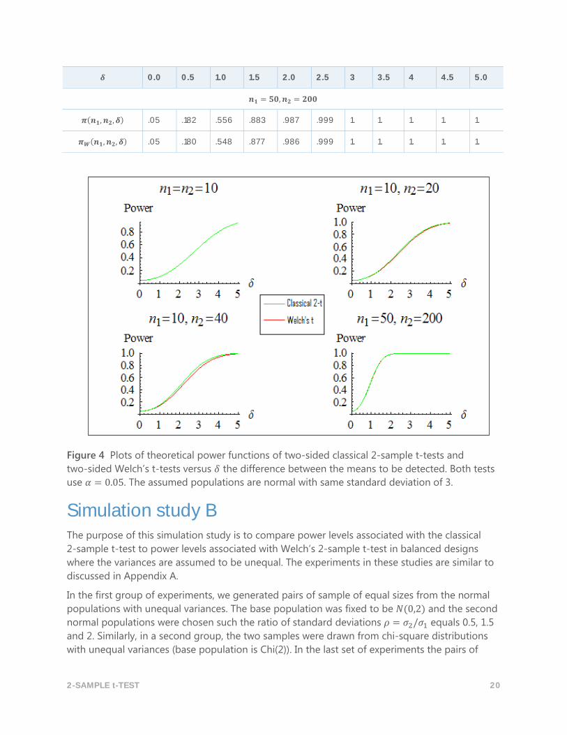
powerful) and therefore it has higher degrees of freedom. The point of the above results,
however, is that if the design is balanced or approximately balanced then the power functions
are identical or approximately identical. The only case where the classical t-test is noticeably
more powerful than the Welch t-test is when the design is markedly unbalanced and the
samples are small. Unfortunately, that also happens to be the case where the classical 2-sample
t-test is particularly sensitive to the assumption of equal variance as shown in Appendix A. As a
result, Welch’s t-test power function is the more reliable function for practical purposes.
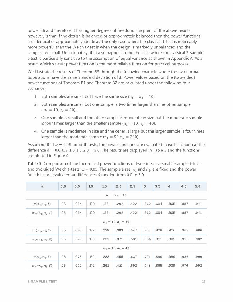
We illustrate the results of Theorem B3 through the following example where the two normal
populations have the same standard deviation of 3. Power values based on the (two-sided)
power functions of Theorem B1 and Theorem B2 are calculated under the following four
scenarios:
1. Both samples are small but have the same size (𝑛1 = 𝑛2 = 10).
2. Both samples are small but one sample is two times larger than the other sample
( 𝑛1 = 10, 𝑛2 = 20).
3. One sample is small and the other sample is moderate in size but the moderate sample
is four times larger than the smaller sample (𝑛1 = 10, 𝑛2 = 40).
4. One sample is moderate in size and the other is large but the larger sample is four times
larger than the moderate sample (𝑛1 = 50, 𝑛2 = 200).
Assuming that 𝛼 = 0.05 for both tests, the power functions are evaluated in each scenario at the
difference 𝛿 = 0.0, 0.5, 1.0, 1.5, 2.0, … 5.0. The results are displayed in Table 5 and the functions
are plotted in Figure 4.
Table 5 Comparison of the theoretical power functions of two-sided classical 2-sample t-tests
and two-sided Welch t-tests, 𝛼 = 0.05. The sample sizes, 𝑛1 and 𝑛2, are fixed and the power
functions are evaluated at differences 𝛿 ranging from 0.0 to 5.0.
𝜹 0.0 0.5 1.0 1.5 2.0 2.5 3 3.5 4 4.5 5.0
𝒏𝟏 = 𝒏𝟐 = 𝟏𝟎
𝝅(𝒏𝟏, 𝒏𝟐, 𝜹) .05 .064 .109 .185 .292 .422 .562 .694 .805 .887 .941
𝝅𝑾(𝒏𝟏, 𝒏𝟐, 𝜹) .05 .064 .109 .185 .292 .422 .562 .694 .805 .887 .941
𝒏𝟏 = 𝟏𝟎, 𝒏𝟐 = 𝟐𝟎
𝝅(𝒏𝟏, 𝒏𝟐, 𝜹) .05 .070 .132 .239 .383 .547 .703 .828 .913 .962 .986
𝝅𝑾(𝒏𝟏, 𝒏𝟐, 𝜹) .05 .070 .129 .231 .371 .531 .686 .813 .902 .955 .982
𝒏𝟏 = 𝟏𝟎, 𝒏𝟐 = 𝟒𝟎
𝝅(𝒏𝟏, 𝒏𝟐, 𝜹) .05 .075 .152 .283 .455 .637 .791 .899 .959 .986 .996
𝝅𝑾(𝒏𝟏, 𝒏𝟐, 𝜹) .05 .072 .142 .261 .419 .592 .748 .865 .938 .976 .992
2-SAMPLE t-TEST 20
𝜹 0.0 0.5 1.0 1.5 2.0 2.5 3 3.5 4 4.5 5.0
𝒏𝟏 = 𝟓𝟎, 𝒏𝟐 = 𝟐𝟎𝟎
𝝅(𝒏𝟏, 𝒏𝟐, 𝜹) .05 .182 .556 .883 .987 .999 1. 1. 1. 1. 1.
𝝅𝑾(𝒏𝟏, 𝒏𝟐, 𝜹) .05 .180 .548 .877 .986 .999 1. 1. 1. 1. 1.
Figure 4 Plots of theoretical power functions of two-sided classical 2-sample t-tests and
two-sided Welch’s t-tests versus 𝛿 the difference between the means to be detected. Both tests
use 𝛼 = 0.05. The assumed populations are normal with same standard deviation of 3.
Simulation study B The purpose of this simulation study is to compare power levels associated with the classical
2-sample t-test to power levels associated with Welch’s 2-sample t-test in balanced designs
where the variances are assumed to be unequal. The experiments in these studies are similar to
discussed in Appendix A.
In the first group of experiments, we generated pairs of sample of equal sizes from the normal
populations with unequal variances. The base population was fixed to be 𝑁(0,2) and the second
normal populations were chosen such the ratio of standard deviations 𝜌 = 𝜎2/𝜎1 equals 0.5, 1.5
and 2. Similarly, in a second group, the two samples were drawn from chi-square distributions
with unequal variances (base population is Chi(2)). In the last set of experiments the pairs of
2-SAMPLE t-TEST 21
samples were generated from the contaminated normal distribution (base population CN(.8,4))
as previously defined in Appendix A.
For each set of experiments, we calculated the simulated power levels (at a given detectable
difference 𝛿) associated with each test for the sample sizes 𝑛 = 𝑛1 = 𝑛2 = 5, 10, 15, 20, 25, 30. In
each experiment, the simulated power level was calculated as the proportion of instances when
the null hypothesis was rejected when it was false. For all the experiments, the difference
between the means was specified in one unit of the standard in the base population (the first of
the two samples). More specifically, we fixed 𝛿 = 1.0 × 𝜎1 = 2.0 because it is relatively small for
all three families of distributions in this study. The simulations results are reported in Table 2.2
and displayed in Figure 2.2a, Figure 2.2b and Figure 2.2c.
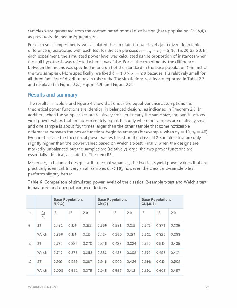
Results and summary
The results in Table 6 and Figure 4 show that under the equal-variance assumptions the
theoretical power functions are identical in balanced designs, as indicated in Theorem 2.3. In
addition, when the sample sizes are relatively small but nearly the same size, the two functions
yield power values that are approximately equal. It is only when the samples are relatively small
and one sample is about four times larger than the other sample that some noticeable
differences between the power functions begin to emerge (for example, when 𝑛1 = 10, 𝑛2 = 40).
Even in this case the theoretical power values based on the classical 2-sample t-test are only
slightly higher than the power values based on Welch’s t-test. Finally, when the designs are
markedly unbalanced but the samples are (relatively) large, the two power functions are
essentially identical, as stated in Theorem B3.
Moreover, in balanced designs with unequal variances, the two tests yield power values that are
practically identical. In very small samples (𝑛 < 10), however, the classical 2-sample t-test
performs slightly better.
Table 6 Comparison of simulated power levels of the classical 2-sample t-test and Welch’s test
in balanced and unequal-variance designs
Base Population: N(0,2)
Base Population: Chi(2)
Base Population: CN(.8,4)
𝑛 𝜎2
𝜎1 .5 1.5 2.0 .5 1.5 2.0 .5 1.5 2.0
5 2T 0.431 0.196 0.152 0.555 0.281 0.215 0.579 0.373 0.335
Welch 0.366 0.166 0.119 0.424 0.250 0.184 0.521 0.320 0.283
10 2T 0.770 0.385 0.270 0.846 0.438 0.324 0.790 0.510 0.435
Welch 0.747 0.372 0.253 0.832 0.427 0.308 0.776 0.493 0.417
15 2T 0.916 0.539 0.387 0.948 0.565 0.424 0.898 0.615 0.508
Welch 0.908 0.532 0.375 0.945 0.557 0.413 0.891 0.605 0.497
2-SAMPLE t-TEST 22
Base Population: N(0,2)
Base Population: Chi(2)
Base Population: CN(.8,4)
20 2T 0.971 0.682 0.497 0.982 0.680 0.521 0.952 0.702 0.573
Welch 0.969 0.677 0.487 0.981 0.676 0.511 0.947 0.697 0.563
25 2T 0.990 0.779 0.591 0.994 0.765 0.605 0.980 0.783 0.641
Welch 0.990 0.777 0.582 0.994 0.762 0.597 0.979 0.778 0.636
30 2T 0.998 0.851 0.675 0.998 0.826 0.676 0.994 0.839 0.699
Welch 0.998 0.849 0.670 0.998 0.824 0.668 0.994 0.836 0.694
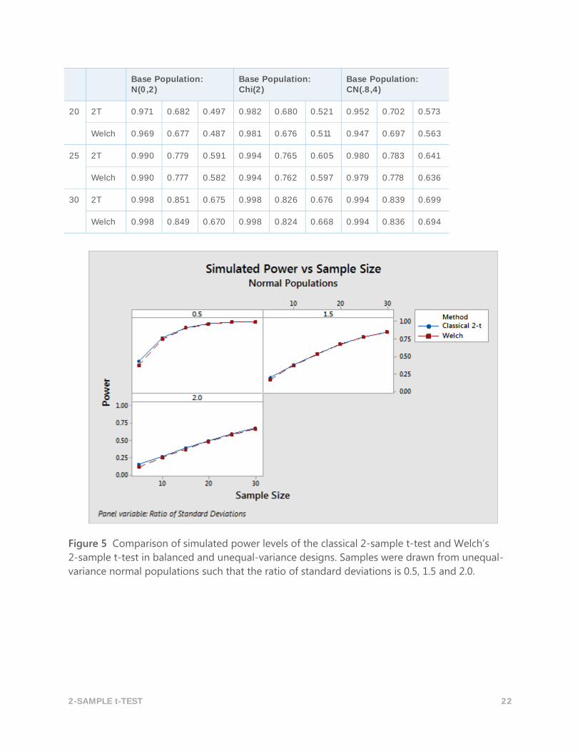
Figure 5 Comparison of simulated power levels of the classical 2-sample t-test and Welch’s
2-sample t-test in balanced and unequal-variance designs. Samples were drawn from unequal-
variance normal populations such that the ratio of standard deviations is 0.5, 1.5 and 2.0.
2-SAMPLE t-TEST 23
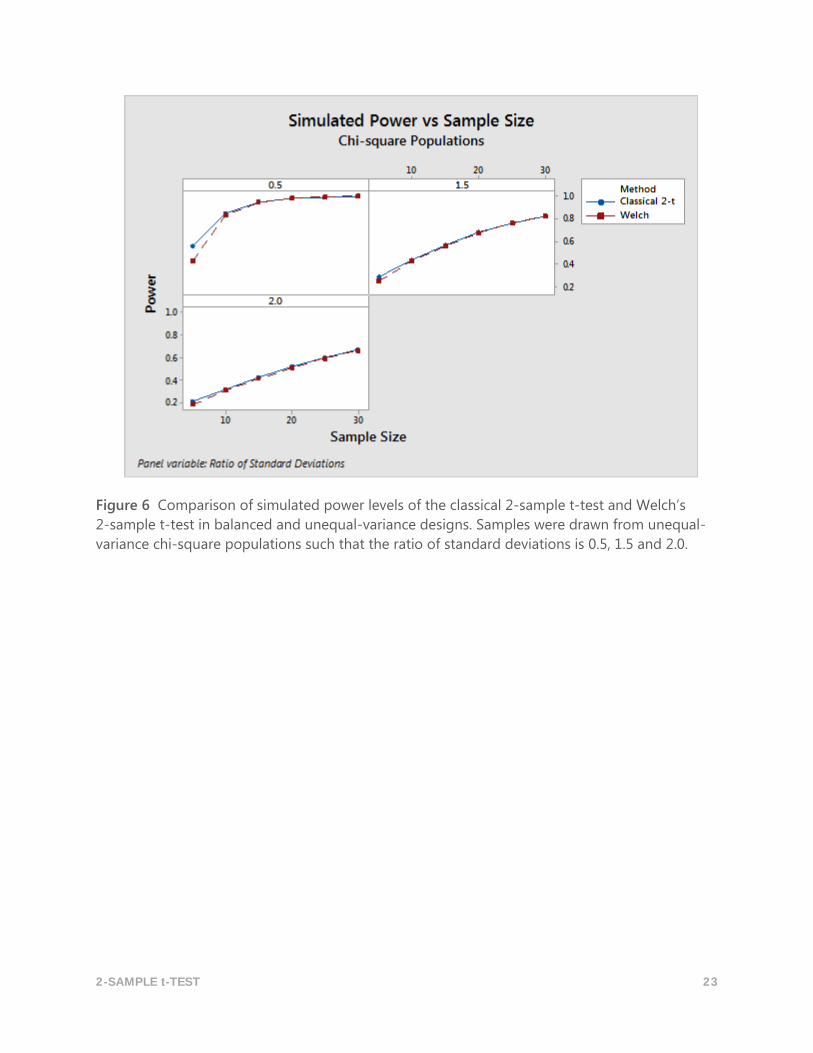
Figure 6 Comparison of simulated power levels of the classical 2-sample t-test and Welch’s
2-sample t-test in balanced and unequal-variance designs. Samples were drawn from unequal-
variance chi-square populations such that the ratio of standard deviations is 0.5, 1.5 and 2.0.
2-SAMPLE t-TEST 24
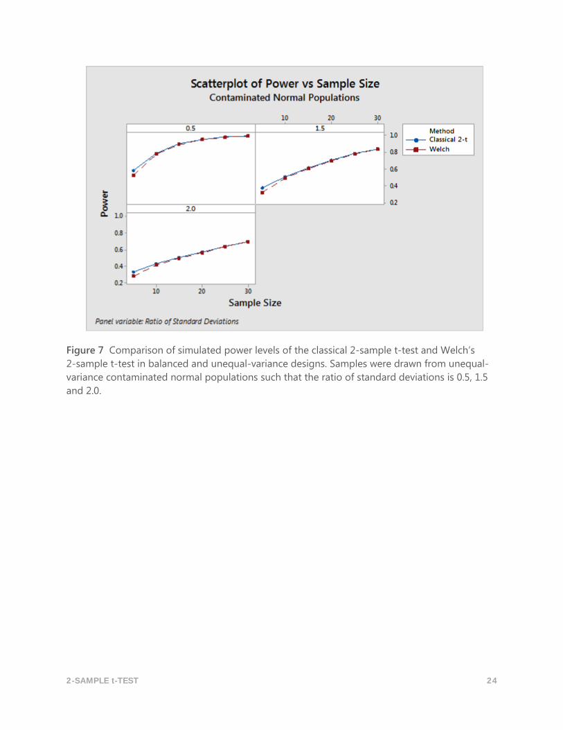
Figure 7 Comparison of simulated power levels of the classical 2-sample t-test and Welch’s
2-sample t-test in balanced and unequal-variance designs. Samples were drawn from unequal-
variance contaminated normal populations such that the ratio of standard deviations is 0.5, 1.5
and 2.0.
2-SAMPLE t-TEST 25
Appendix C: Power and sample size and sensitivity to normality In the Assistant, the power analysis for comparing the means of two populations is based upon
the power function of the Welch t-test. Should this function be sensitive to the normal
assumption under which it is derived, the power analysis may yield erroneous conclusions. For
this reason, we conducted a simulation study to examine the sensitivity of this function to the
normal assumption. Sensitivity is assessed as the consistency between simulated power levels
and power levels calculated from the theoretical power function when samples are generated
from nonnormal distributions. The normal distribution serves as the control population because,
according to Theorem B2, simulated power levels and theoretical power levels are closest when
samples are generated from the normal populations.
Simulation study C The study is conducted in three parts using three distributions: normal, chi-square, and the
contaminated normal distribution. Refer to Appendix A for more details. For each part of the
study, the simulated power is calculated (for the given sample sizes n1 and n2 at a given
detectable difference δ) as the proportion of instances when the null hypothesis was rejected
when it was false. In all the cases the difference to be detected is specified in one unit of the
standard in the base population. That is δ = 1.0 × σ1 = 2.0 for all three families of distributions
in this study. The theoretical power values based on Welch’s t-test are calculated as well for
comparison.
Simulation results and summary The results show that for relatively small sample sizes the power function of the Welch t-test is
robust against the normality assumption. In general, when the minimum size of the two samples
is as low as 15, the simulated power values are near their corresponding targeted theoretical
power levels (see Tables 7-10 and Figures 8-10).
Tables 7-10 show the simulated power levels of a two-sided Welch t-test with 𝛼 = 0.05 based on
pairs of samples generated from normal population, skew populations (chi-square), and
contaminated normal populations. The pairs of samples are from the same family of distribution
but the variances of the parent populations are not necessarily equal. The theoretical power
values were calculated for comparison.
2-SAMPLE t-TEST 26
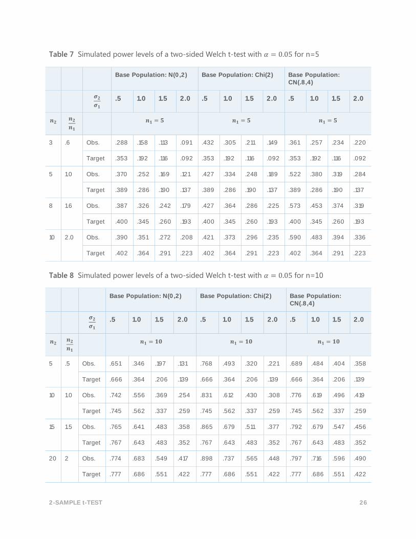
Table 7 Simulated power levels of a two-sided Welch t-test with 𝛼 = 0.05 for n=5
Base Population: N(0,2) Base Population: Chi(2) Base Population: CN(.8,4)
𝝈𝟐
𝝈𝟏 .5 1.0 1.5 2.0 .5 1.0 1.5 2.0 .5 1.0 1.5 2.0
𝒏𝟐 𝒏𝟐
𝒏𝟏 𝒏𝟏 = 𝟓 𝒏𝟏 = 𝟓 𝒏𝟏 = 𝟓
3 .6 Obs. .288 .158 .113 .091 .432 .305 .211 .149 .361 .257 .234 .220
Target .353 .192 .116 .092 .353 .192 .116 .092 .353 .192 .116 .092
5 1.0 Obs. .370 .252 .169 .121 .427 .334 .248 .189 .522 .380 .319 .284
Target .389 .286 .190 .137 .389 .286 .190 .137 .389 .286 .190 .137
8 1.6 Obs. .387 .326 .242 .179 .427 .364 .286 .225 .573 .453 .374 .319
Target .400 .345 .260 .193 .400 .345 .260 .193 .400 .345 .260 .193
10 2.0 Obs. .390 .351 .272 .208 .421 .373 .296 .235 .590 .483 .394 .336
Target .402 .364 .291 .223 .402 .364 .291 .223 .402 .364 .291 .223
Table 8 Simulated power levels of a two-sided Welch t-test with 𝛼 = 0.05 for n=10
Base Population: N(0,2) Base Population: Chi(2) Base Population: CN(.8,4)
𝝈𝟐
𝝈𝟏 .5 1.0 1.5 2.0 .5 1.0 1.5 2.0 .5 1.0 1.5 2.0
𝒏𝟐 𝒏𝟐
𝒏𝟏 𝒏𝟏 = 𝟏𝟎 𝒏𝟏 = 𝟏𝟎 𝒏𝟏 = 𝟏𝟎
5 .5 Obs. .651 .346 .197 .131 .768 .493 .320 .221 .689 .484 .404 .358
Target .666 .364 .206 .139 .666 .364 .206 .139 .666 .364 .206 .139
10 1.0 Obs. .742 .556 .369 .254 .831 .612 .430 .308 .776 .619 .496 .419
Target .745 .562 .337 .259 .745 .562 .337 .259 .745 .562 .337 .259
15 1.5 Obs. .765 .641 .483 .358 .865 .679 .511 .377 .792 .679 .547 .456
Target .767 .643 .483 .352 .767 .643 .483 .352 .767 .643 .483 .352
20 2 Obs. .774 .683 .549 .417 .898 .737 .565 .448 .797 .716 .596 .490
Target .777 .686 .551 .422 .777 .686 .551 .422 .777 .686 .551 .422
2-SAMPLE t-TEST 27
Table 9 Simulated power levels of a two-sided Welch t-test with 𝛼 = 0.05 for n=15
Base Population: N(0,2) Base Population: Chi(2) Base Population: CN(.8,4)
𝜎2
𝜎1 .5 1.0 1.5 2.0 .5 1.0 1.5 2.0 .5 1.0 1.5 2.0
𝑛2 𝑛2
𝑛1 𝑛1 = 15 𝑛1 = 15 𝑛1 = 15
8 .53 Obs. .857 .569 .342 .229 .871 .651 .421 .293 .853 .632 .505 .428
Target .861 .568 .338 .221 .861 .568 .338 .221 .861 .568 .338 .221
15 1.0 Obs. .906 .745 .535 .368 .942 .763 .563 .415 .891 .760 .611 .500
Target .910 .753 .541 .379 .910 .753 .541 .379 .910 .753 .541 .379
23 1.53 Obs. .928 .831 .667 .502 .975 .858 .676 .517 .898 .825 .698 .572
Target .925 .830 .670 .509 .925 .830 .670 .509 .925 .830 .670 .509
30 2.0 Obs. .933 .861 .737 .589 .984 .903 .750 .598 .902 .847 .742 .619
Target .931 .863 .736 .589 .931 .863 .736 .589 .931 .863 .736 .589
Table 10 Simulated power levels of a two-sided Welch t-test with 𝛼 = 0.05 for n=20
Base Population: N(0,2) Base Population: Chi(2) Base Population: CN(.8,4)
𝝈𝟐
𝝈𝟏 .5 1.0 1.5 2.0 .5 1.0 1.5 2.0 .5 1.0 1.5 2.0
𝒏𝟐 𝒏𝟐
𝒏𝟏 𝒏𝟏 = 𝟐𝟎 𝒏𝟏 = 𝟐𝟎 𝒏𝟏 = 𝟐𝟎
10 .5 Obs. .938 .687 .426 .275 .920 .698 .486 .333 .923 .716 .568 .476
Target .941 .686 .424 .277 .941 .686 .424 .277 .941 .686 .424 .277
20 1.0 Obs. .971 .866 .672 .485 .981 .858 .670 .506 .952 .856 .696 .567
Target .971 .869 .673 .489 .971 .869 .673 .489 .971 .869 .673 .489
30 1.5 Obs. .977 .923 .791 .629 .995 .932 .785 .631 .960 .908 .798 .662
Target .978 .922 .791 .628 .978 .922 .791 .628 .978 .922 .791 .628
40 2.0 Obs. .983 .950 .858 .724 .998 .966 .864 .726 .958 .929 .845 .725
Target .981 .945 .854 .719 .981 .945 .854 .719 .981 .945 .854 .719
2-SAMPLE t-TEST 28
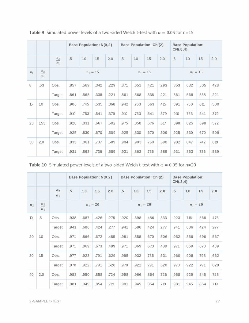
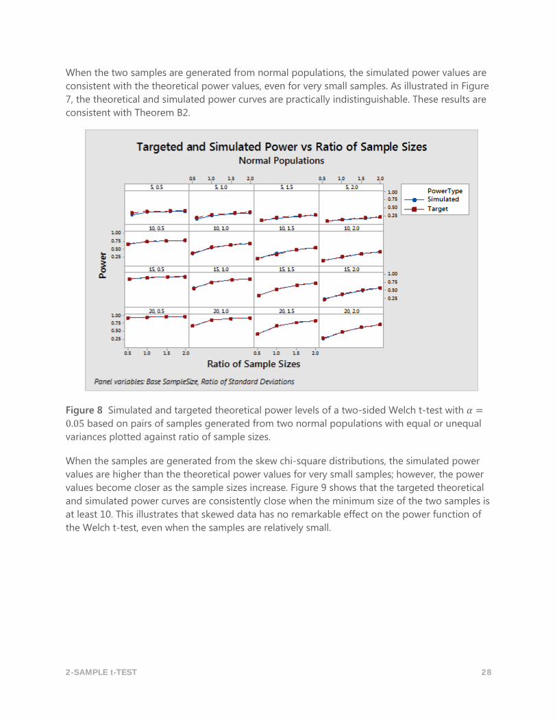
When the two samples are generated from normal populations, the simulated power values are
consistent with the theoretical power values, even for very small samples. As illustrated in Figure
7, the theoretical and simulated power curves are practically indistinguishable. These results are
consistent with Theorem B2.
Figure 8 Simulated and targeted theoretical power levels of a two-sided Welch t-test with 𝛼 =
0.05 based on pairs of samples generated from two normal populations with equal or unequal
variances plotted against ratio of sample sizes.
When the samples are generated from the skew chi-square distributions, the simulated power
values are higher than the theoretical power values for very small samples; however, the power
values become closer as the sample sizes increase. Figure 9 shows that the targeted theoretical
and simulated power curves are consistently close when the minimum size of the two samples is
at least 10. This illustrates that skewed data has no remarkable effect on the power function of
the Welch t-test, even when the samples are relatively small.
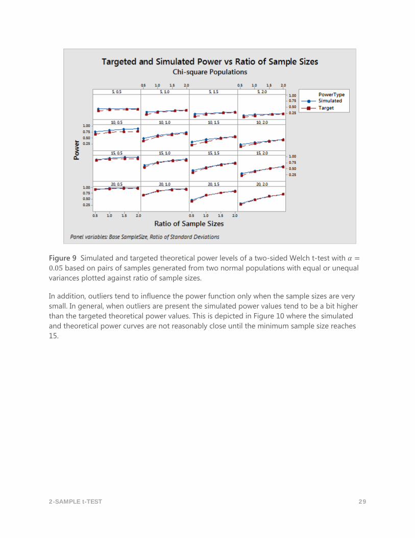
2-SAMPLE t-TEST 29
Figure 9 Simulated and targeted theoretical power levels of a two-sided Welch t-test with 𝛼 =
0.05 based on pairs of samples generated from two normal populations with equal or unequal
variances plotted against ratio of sample sizes.
In addition, outliers tend to influence the power function only when the sample sizes are very
small. In general, when outliers are present the simulated power values tend to be a bit higher
than the targeted theoretical power values. This is depicted in Figure 10 where the simulated
and theoretical power curves are not reasonably close until the minimum sample size reaches
15.
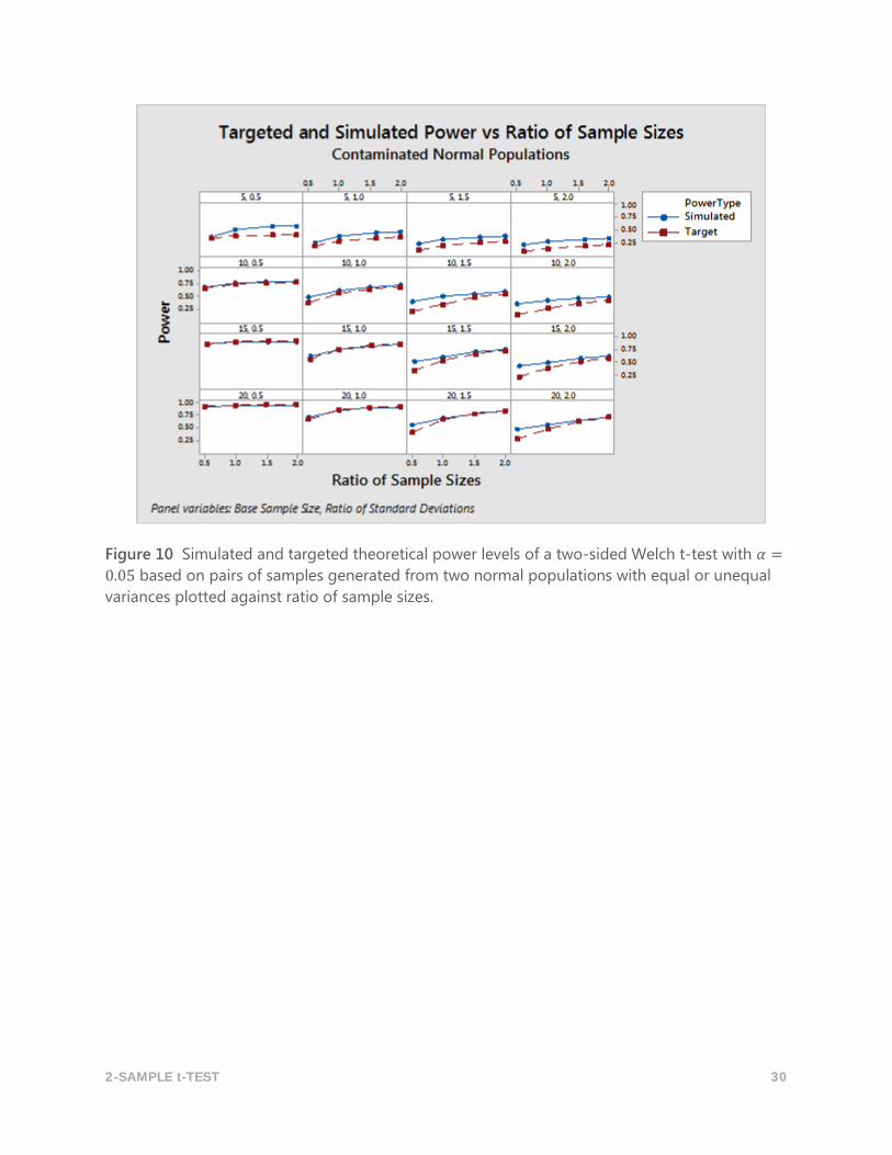
2-SAMPLE t-TEST 30
Figure 10 Simulated and targeted theoretical power levels of a two-sided Welch t-test with 𝛼 =
0.05 based on pairs of samples generated from two normal populations with equal or unequal
variances plotted against ratio of sample sizes.
2-SAMPLE t-TEST 31
Appendix D: Proof of theorem B2 For the two-sample model, Welch’s approach for deriving the distribution of the test statistic
𝑡𝑤(𝑥, 𝑦) =�̅� − �̅� − 𝛿
√𝑠1
2
𝑛1+
𝑠22
𝑛2
under the null hypothesis is based upon an approximation of the distribution of
𝑉 =𝑠1
2
𝑛1+
𝑠22
𝑛2
as proportional to a chi-square distribution. More specifically,
𝑑𝑊𝑉
𝜎12
𝑛1+
𝜎22
𝑛2
is approximately distributed as a chi-square distribution with 𝑑𝑊 degrees of freedom where
𝑑𝑊 =(
𝜎12
𝑛1+
𝜎22
𝑛2)
2
𝜎14
𝑛12(𝑛1 − 1)
+𝜎2
4
𝑛22(𝑛2 − 1)
(Note that in a one-sample setting this reduces to the well known classical result that (𝑛 − 1)𝑠2/
𝜎2~𝜒𝑛−12 )
Consider the test of the null hypothesis 𝐻𝑜: 𝜇1 = 𝜇2 (or equivalently 𝛿 = 0) against the
alternative 𝐻𝐴: 𝜇1 ≠ 𝜇2 (or equivalently 𝛿 ≠ 0)
Under the null hypothesis, the power function
𝜋(𝑛1, 𝑛2, 𝛿) = 𝜋(𝑛1, 𝑛2, 0) = 1 − Pr (−𝑡𝑑𝑊
𝛼/2≤
�̅� − �̅�
√𝑉≤ 𝑡𝑑𝑊
𝛼/2) ≈ 𝛼
where 𝑡𝑑𝛼denotes the 100 𝛼 upper percentile point of the t-distribution with 𝑑 degrees of
freedom.
Under the alternative hypothesis,
�̅� − �̅�
√𝑉=
�̅� − �̅� − 𝛿
√𝜎1
2
𝑛1+
𝜎22
𝑛2
+𝛿
√𝜎1
2
𝑛1+
𝜎22
𝑛2
√𝑑𝑊𝑉
𝑑𝑊 (𝜎1
2
𝑛1+
𝜎22
𝑛2)
2-SAMPLE t-TEST 32
has the approximate non-central t distribution with 𝑑𝑊 degrees of freedom with non-centrality
parameter
𝜆𝑊 =𝛿
√𝜎12/𝑛1 + 𝜎2
2/𝑛2
because as stated earlier
𝑑𝑊𝑉
𝜎12
𝑛1+
𝜎22
𝑛2
is approximately distributed as a chi-square distribution with 𝑑𝑊 degrees of freedom, and
�̅� − �̅� − 𝛿
√𝜎1
2
𝑛1+
𝜎22
𝑛2
is distributed as a standard normal distribution.
It follows that under the alternative,
𝜋(𝑛1, 𝑛2, 𝛿) = 1 − Pr (−𝑡𝑑𝑊
𝛼/2≤
�̅� − �̅�
√𝑉≤ 𝑡𝑑𝑊
𝛼/2) ≈ 1 − 𝐺𝑑𝑊,𝜆𝑊
(𝑡𝑑𝑊
𝛼/2) + 𝐺𝑑𝑊,𝜆𝑊
(−𝑡𝑑𝑊
𝛼/2)
where 𝐺𝑑𝑊,𝜆(. ) is the C.D.F of the non-central t distribution with 𝑑𝑊 degrees of freedom and
non centrality parameter 𝜆 as given above.
2-SAMPLE t-TEST 33
Appendix E: Proof of theorem B3 First, note that 𝑑𝑊 can be rewritten as
𝑑𝑊 =(
1𝑛1
+𝜌2
𝑛2)
2
1𝑛1
2(𝑛1 − 1)+
𝜌4
𝑛22(𝑛2 − 1)
where 𝜌 = 𝜎1/𝜎2.
Similarly, the non-centrality parameter associated with the Welch t-test power function can also
be written as
𝜆𝑊 =𝛿/𝜎1
√1/𝑛1 + 𝜌2/𝑛2
Under the assumption of equal variance, the non-centrality parameters associated with the
power functions of the classical 2-sample t-test and the Welch test coincide. That is
𝜆 = 𝜆𝑊 =𝛿
𝜎√1/𝑛1 + 1/𝑛2
where 𝜎 is the common variance of the two populations. Thus, the only difference in the power
functions of the two tests resides in the difference between their respective degrees of freedom.
But, under the equal variance assumption, the degrees of freedom associated with the Welch
t-test power function becomes
𝑑𝑊 =(
1𝑛1
+1
𝑛2)
2
1𝑛1
2(𝑛1 − 1)+
1𝑛2
2(𝑛2 − 1)
=(𝑛1 + 𝑛2)2(𝑛1 − 1)(𝑛2 − 1)
𝑛12(𝑛1 − 1) + 𝑛2
2(𝑛2 − 1)
By Theorem 1, the degrees of freedom related to the power function of the classical 2-sample
t-test is 𝑑𝐶 = 𝑛1 + 𝑛2 − 2. After some algebraic manipulations, we have
𝑑𝐶 − 𝑑𝑊 =(𝑛1 − 𝑛2)2(𝑛1 + 𝑛2 − 1)2
𝑛12(𝑛1 − 1) + 𝑛2
2(𝑛2 − 1)≥ 0
The fact that 𝑑 − 𝑑𝑊 ≥ 0 is not surprising because we know that under the assumption of
equality of variances the classical 2-sample t-test is UMP (uniformly most powerful), as a result
one should expect the degrees of freedom associated with its power function to be higher.
Now, if 𝑛1~𝑛2 then 𝑑~𝑑𝑊 and as a result the power functions have the same order of
magnitude. In particular, the power functions of the two tests are identical if 𝑛1 = 𝑛2. This proves
the first part of theorem 2.3.
If 𝑛1 ≠ 𝑛2, then 𝑑𝐶 − 𝑑𝑊 > 0 so that the Welch t-test has less power than the classical 2-sample
t-test.
2-SAMPLE t-TEST 34
In addition, if the samples are large, that is if 𝑛1 → ∞ and 𝑛2 → ∞ then 𝑑𝐶 → ∞ and 𝑑𝑊 → ∞ so
that the asymptotic distribution of the test statistics associated with both tests is the standard
normal distribution. Thus, the tests are asymptotically equivalent and yield the same asymptotic
power function.
© 2015, 2017 Minitab Inc. All rights reserved.
Minitab®, Quality. Analysis. Results.® and the Minitab® logo are all registered trademarks of Minitab,
Inc., in the United States and other countries. See minitab.com/legal/trademarks for more information.