Embed Size (px)
Citation preview

REPORT DOCUMENTATION PAGE i� Form ApprovedJ 0MB No. 0704-0 188Publ( reporting burdOn
40r this collection o� n�0tiYiaton n ettinsated tc a�e.age I hour oei i�i�Ot'5e. inciJding the tiMC lOt re�'iewing inStrUCIiOr'I. searching Casting data sources.
g.th.r�ng and maintaining the data needed, and ccmnplenng and res.�eii�g �rre c�JIecton o� ir.lormetiOn. Send comments regarding this burden estimate or any other aspeCt 01 thucollectaon 01 ,nlotmatrOfi. including suggestions lot reducing this bunoen. to A'ashngton .ueaoouarters Services. Directorate f�r inlormatron ODe'ations aria RepOrts. 1715 JeflersonDevil Highmay. Suite 1204. Arlington. VA 222024302, and to the Ollice ol 'Aenagernent and � Pnperwcrk Reduction Project (0704.0188). Washington. DC 20503.
1. AGENCY USE ONLY (Leave blank) 2. REPORT DATE 3. REPORT TYPE AND DATES COVERED10 Aug 1994 Final 25 Jun 1990 - 10 Aug 1994
4. TITLE AND SUBTITLE r 5. FUNDING NUMBERSArtificial Neural Network Metamodels of Stochastic I ()Computer Simulations
6. AUTHOR(S) AD- A285 951Robert Allen Kilmer 1111111 iiii 1111111 1111 El ill 1�Il 1111
7. PERFORMING ORGANIZATION NAME(S) AND ADDRESS(ES) 8. PERFORMING ORGANIZATIONREPORT NUMBER
Robert Allen Khmer�%.4 ___ Department of Industrial Engineering(� University of Pittsburgh, Pittsburgh, PA 15261
(V) �- 9. SPONSORING/MONITORING AGENCY NAME(S) AND ADDRESS(ES) 10.SP N O�LN .
I �- Department of the Army �U.S. Army Soldier Support Center � 4 1994
___ Fort Benjamin Harrison, IN 46216-5170 �i
11. SUPPLEMENTARY NOTESPrepared in support of U.S. Army fully funded Ph.D. Progra
¶2a. DISTRIBUTION / AVAILABILITY STATEMENT 12b. DISTRIBUTION CODEApproved for Public Release; Distribution is Unlimited A
13. ABSTRACT (Maxin'.urn200 words) A computer simulation model can be thought of as a re 1 ationthat connects input parameters to output measures. Since these models can becomecomputationally expensive in terms of processing time and/or memory requirements,there are many reasons why it would be beneficial to be able to approximate these
if) models in a computationally expedient manner. This research examines the use ofartificial neural networks (ANN), to develop a metamodel of computer simulations.0 The development and use of the Baseline ANN Metamodel Approach is provided and isshown to outperform traditional regression approaches. The results provide a solidfoundation and methodological direction for developing ANN metamodels to perform
complex tasks such as simulation "optimization," sensitivity analysis, and simulationaggregation/reduction.
".4
14. SUBJECT TERMS 15. NUMBER OF PAGES�44 234Artiricial Neural Networks, Computer Simulation Metamodel, 16. PRICE CODE
Regression, Response Surface Methods, Simulation Optimization
17. SECURITY CLASSIFICATION ¶8. SECURITY CLASSIFICATION 19. SECURITY CLASSIFICATION 20. LIMITATION OF ABSTRACTOF REPORT OF THIS PAGE OF ABSTRACT
UNCLASS UNCLASS UNCLASS UNLIMITED
NSN 7540.O1-280-550a Standard Form 298 (�ev. 2-89)P�esCribed by �NSl Sid 239.'!298*1C2
ARTIFICIAL NEURAL NETWORK METAMODELS
OF STOCHASTIC COMPUTER SIMULATIONS
by
Robert Allen Kilmer
B.S. in Education Mathematics, Indiana University of Pennsylvania
M.S. in Operations Research, Naval Postgraduate School
Submitted to the Graduate Faculty
of the School of Engineering
in partial fulfillment of
the requirements for the degree of
Doctor
Acce, ion For I of
NTIS . .. PhilosophyD TC IC
IJ , .
University of Pittsburgh
i , ,1994
-...... The author grants permissionto reproduce single copies.
Signed
COMMITTEE SIGNATURE PAGE
This dissertation was presented
by
Robert A. Kilmer
It was defended on
4 August 1994
and approved by
Committee MemberAlice Smith. Assistant Professor of Industrial Engineering
Commntee MemberDavid Tate, Assistant Professor of Industrial Engineering
CmV i ee Mem rWo•• lfe, Chairman and Professor of Industrial Engineering
/tomm-ittee Membeý
"Jei~d M~y, Professor of Business'-." t° I L
Committee MemberPaul Fischbeck. Assistant Professor of Decision Science and Public Policy
ii

ACKN()WLEI)(;MENTS
I am indebted to my advisor, Dr. Larry Shuman, for his support, guidance and
suggestions throughout the doctoral process. I am thankful to Dr. Alice Smith and Dr.
David Tate for their many hours spent in discussing various aspects of this research. I am
also appreciative of the other committee members, Dr. Wolfe, Dr. Fishbeck and Dr. May
for their helpful comments and suggest;
I thank all of the faculty, staff and students at the University of Pittsburgh that
provided support and encouragement throughout the cour ;e of this research. In particular
Jan Twomey, Cenk Tunasar, Rich Puerzer, Gary Bums, Mary Ann Holbý-ir' and Jim
Segneff were especially supportive.
For the opportunity to pursue post-baccalaureate studies, I am indebted to the
United States Army. I also thank Colonel James Kays and the personnel of the
Department of Systems Engineering, United States Military Academy, for their
encouragement and time to permit the completion of this document.
I thank my wife, Sandy and our children Beth, Meg and Todd for their love and
understanding throughout the entire graduate school experience.
I thank God for the privilege and honor of obtaining a Doctorate of Philosophy
degree and I dedicate this document to the memory of my father, William Ralph Kilmer.
mi

ABSTRACT
Signature
ARTIFICIAL NEURAL NETWORK METAMODELS OFSTOCHASTIC COMPUTER SIMULATIONS
Robert A. Kilmer, Ph.D.
University of Pittsburgh
A computer simulation model can be thought of as a relation which connects input
parameters to output measures. Since these models can become computationally
expensive in terms of processing time and/or memory requirements, there are many
reasons why it would be beneficial to be able to approximate these models in a
computationally expedient manner. This research examines the use of artificial neural
networks (ANN), to develop a metamodel of computer simulations. The development and
use of the Baseline ANN Metamodel Approach is provided and is show, n to outperform
traditional regression approaches. The results provide a solid foundation and
methodological direction for developing ANN metarnodels to perfon-n complex tasks such
as simulation 'optimization'. sensitivity analysis, and simulation aggreit-±ion/rt,.jction.
iv

DESCRIPTORS
Approximation Artificial Neural Nemorks
Backpropagation Computer Simulation
Confidence Intervals Discrete-event Simulation
Estimation Metw-nodeling
Multiple Linear Regression Non-Linear Rearession
Non-Parametric Regression Prediction Intervals
Regression Response Surface Methodologies
Sensitivity Analysis Simulation Aggre-gation
Simulation Optimization Simulation Reduction
Stochastic Simulation Terminating Simulation

TABLE OF CONTENTSPage
ACKNOW LEDGM ENTS ........................................................................................ iii
ABSTRA CT ................................................................................................................... iv
LIST OF FIGURES .................................................................................................... xi
LIST OF TABLES ................................................................................................... xvi
NOM ENCLATURE (SYM BOLS) ........................................................................... xix
1.0 IN-TRODU CTION ................................................................................................ I
1.1 Problem Statem ent ............................................................................................. 1
1.2 hImportance of Computer Sim ulation ............................................................. 4
1.3 Problem s with Computer Simulations ............................................................ 5
1.4 Need for Better Approximations to Computer Simulation Models .................. 6
1.5 Using ANN to Approximate Computer Simulations ....................................... 8
1.6 Overview of the Dissertation ............................................................................ 10
1.7 Restrictions of the Research ............................................................................. 11
1.8 Summu-ary ...................................................................................................... 12
2.0 LITERATURE REVIEW .................................................................................. 13
2.1 Computer Sim ulation .................................................................................. 13
2.2 Artificial Neural Networks ........................................................................... 16
2.3 M etam odels ..................................................................................................... 31
\i1

Page
2.3.1 Linear Regression ............................................................................. 33
2.3.2 Response Surface Methodology (RSM) .............................................. 35
2.3.3 T aguchi M odels 7.................................................................................... 37
2.3.4 A pproxim ation T heory ........................................................................... 31
2.4 Sum m ary ..................................................................................................... 39
3.0 RESEARCH METHODOLOGY, ISSUES AND TOOLS .................................. 41
3.1 Methodology of Research ........................................................................... 41
3.1.1 Basic Research Tasks ......................................................................... 41
3.1.2 Assumptions and Restrictions of the Research ................................... 43
3.2 Research Issues ........................................................................................... 45
3.3 R esearch Tools ........................................................................................... 45
3.3.1 SIMAN/CINEMA Simulation Language ............................................ 46
3.3.2 BrainMaker Neural Network Computing Package .............................. 47
3.4 Surru-nary .................................................................................................... . . 52
4.0 DEVELOPMENT PROBLEM - INITIAL EXPERIMENTS INAPPROXIMATING AN (s,S) INVENTORY SYSTEM ................................... 53
4.1 Description of the (s,S) Inventory System ........................................................ 53
4.2 Computer Simulation of the Inventory System ........................................... 56
4.3 Experiments with Two Simulation Input Parameters .................................... 66
4.3.1 Experiment #1: Presentation Methods of Output Measures ................ 69
4.3.2 Experiment #2: Predicting Descriptive Statistics Typically Produced byComputer Simulations (Mean. Standard Deviation, Min. and Max) .... 76
vii
Page
4.4 Synopsis of Conclusions from Initial Experiments ............................................. 90
4.5 S um m ary ................................................................................................... . . 9 1
5.0 DEVELOPMENT PROBLEM - FINAL SET OF EXPERIMENTS INAPPROXIMATING AN (s.S) INVENTORY SYSTEM ................................... 92
5.1 Experiments with Four Simulation Input Parameters .................................... 93
5.2 Experiment #3: Detenrmining the Number of Hidden Nodes Needed toPredict a Simulation Output Measure ....................................................... 99
5.3 Experiment #4: Predicting Mean Cost of the (s,S) Inventory Simulation ......... 103
5.3.1 Examining Four Input Dimension ANN Results on a 2D im ensional Surface ......................................................................... 103
5.3.2 Results of Experim ent 4 ....................................................................... 105
5.4 Experiment #5: Predicting the Variance of Mean Cost of the Four ParameterInventory Sim ulation ................................................................................... 113
5.4.1 Examining Four Input Dimension ANN Variance Results ona 2 D im ensional Surface .................................................................... 114
5.4.2 R osults of Experim ent 5 ...................................................................... 115
5.5 Experiment #6: Comparing Prediction Intervals from Direct Simulation withthose Developed from ANN Approximations of the Computer Simulation ................... 120
5.6 Synopsis of Conclusions from Experiments 3 through 6 ................................ 123
5.7 Sum m ary ....................................................................................................... 125
6.0 BASELINE ANN METAMODEL APPROACH .................................................. 127
6.1 Description of the Basehine ANN Metamodel Approach ................................. 127
6.1.1 Phase I of the Baseline ANN Metamodel Approach ............................. 127
viii
Page
6.1.2 Phase 2 of the Baseline ANN Metamodel Approach ............................. 129
6.1.3 Phase 3 of the Baseline ANN Metamodel Approach ................. 131
6.2 Assumptions of the Baseline ANN Metamodeling Approach ...................... 132
6.3 Limitations of the Baseline ANN Metamodefing Approach ................ 133
6.4 Justification of the Baseline ANN Metamodeling Approach ............................ 134
6.5 Suim nary ....................................................................................................... 135
7.0 DEMONSTRATION PROBLEM - AN EMERGENCY DEPARTMENT (ED)S Y ST E M ........................................................................................................... 136
7.1 Description of the ED System ........................................................................ 136
7.2 Computer Sim ulation of ED System ............................................................... 136
7.2.1 Physical Layout of the ED ............................... 138
7.2.2 Patient Representation in the ED .......................................................... 138
7.2.3 W orkers in the ED ............................................................................... 14 1
7.2.4 V alidation of the Sim ulation ................................................................. 141
7.3 Demonstration of the Baseline ANN Metamodel Approach ........................... 142
7.3.1 Phase 1 of the Baseline ANN Metamodel Approach ............................. 142
7.3.2 Phase 2 of the Baseline ANN Metamodel Approach ............................. 146
7.3.3 Phase 3 of the Baseline ANN Metamodel Approach ............................. 148
7.4 Results of ED System Dem onstration ............................................................. 157
7.5 Sumrunary ....................................................................................................... 158
8.0 SUMMARY AND CONCLUSIONS ................................................................ 1601
ix

Page
8.1 Tie Baseline ANN M etamodeling Approach .................................................. 160
8.2 The Performance of the Baseline ANN Metamodeling Approach ............. 161
8.3 M ajor Contributions of the D issertation ......................................................... 162
8.4 Future Research Directions ................................... 162
8.4.1 Improvements of the Baseline ANN Metarnodel Approach ................... 162
S.4.2 Extensions of the Baseline ANN Metamodel Approach ........................ 165
8.4.3 Applications of the Baseline ANN Metamodel Approach ...................... 166
8.5 Sumrumary ....................................................................................................... 169
APPENDIX A DEVELOPMENT PROBLEM 2 PARAMETER INVENTORYSIMULATION COMPUTER PROGRAMS AND RESULTS .................................. 170
APPENDIX B DEVELOPMENT PROBLEM 4 PARAMETER INVENTORYSIMULATION COMPUTER PROGRAMS AND RESULTS ................................... 190
APPENDIX C DEMONSTRATION PROBLEM ED RESULTS ............................... 204
B IB L IO G RA PH Y ....................................................................................................... 221
• 1 I I I I II I
LIST OF FI(URES
Figure No. Page
1 Mechanistic and Empirical Modeling Approaches ................................................... 2
2 Constucting Metamodels of Computer Simulations ........................................... 3
3 A T ypical A N N N ode ...................................................................................... 19
4 Typical Feedforward ANN .................................................................................. 2()
5 ANN Training: Stage One ................................................................................ 22
6 ANN Trai ,g: Stage Two ................................................................................. 2-
7 A N N T esting ................................................................................................. . . 23
8 ANrN Operation ............................................................................................... 24
9a Direct Simulation at 420 Points ......................................................................... 63
9b Regression Based on 36 Points ......................................................................... 64
9c ANN Based on 36 Points .................................................................................. 65
10 Training and Testing Points for Experiments I and 2 .......................................... 69
11 Schematic of ANN Used for Experiment I ......................................................... 71
12 Training Set Results for Experiment I ................................................................ 72
13 Presentations Required to Terminate Training for Experiment I ....................... 73
14 Internal Test Set Results for Experiment I ...................................................... 74
15 External Test Set Results for Experiment I ...................................................... 75
16 Combined Test Set Results for Experiment 1 .................................................... 75
17 Training Set Results for Experiment 2 for Mean Cost ........................................ 78
18 Training Set Results for Experiment 2 for Standard Deviation of Cost .............. 7S
xi
Page
19 Training Set Results for Experiment 2 for Minimum Value of Cost ................... 79
20 Training Set Results for Experiment 2 for Maximum Value of Cost .................. 79
21 Presentations Required to Terminate Training for Experiment 2 ...................... X0
22 Test Set Results for Experiment 2 for Mean Cost .............................................. 81
23 Test Set Results for Experiment 2 for Standard Deviation of Cost ..................... 2
24 Test Set Results for Experiment 2 for Minimum Value of Cost ......................... 82
25 Test Set Results for Experiment 2 for Maxinum Value of Cost ........................ 83
26 Comparison of Experiment I and Experiment 2 Training Set Results forPredicting Mean Value of Cost (C) for Presentation Method 1 .................... 84
27 Comparison of Experiment I and Experiment 2 Training Set Results forPredicting Mean Value of Cost (C) for Presentation Method 2 .................... 85
28 Comparison of Experiment I and Experiment 2 Training Set Results forPredicting Mean Value of Cost (C) for Presentation Method 3 ................... 85
29 Comparison of Experiment 1 and Experiment 2 Test Set Results forPredicting Mean Value of Cost (C) for Presentation Method 1 ..................... 86
30 Comparison of Experiment I and Experiment 2 Test Set Results forPredicting Mean Value of Cost (C) for Presentation Method 2 .................... 86
31 Comparison of Experiment I and Experiment 2 Test Set Results forPredicting Mean Value of Cost (C) for Presentation Method 3 .................... 87
32 Results of Experiment 3 for Training Set M (Unshuffled Data) ............................ 101
33 Results of Experiment 3 for ANN Trained on Averages (PM 1) ...................... 102
34 Results of Experiment 3 for ANN Trained on Individual Replications (PM 4) ...... 102
35 Surface Plot of Mean Cost Based on Training Set F ......................... 105
xii
Page
36 Number of Presentations of the Training Data To Reach the Best TrainedNetwork in Experiment 4 for Training Sets Based on 10 Replications ............... 106
37 Results of Presentation Methods I and 4 with WO Replicationsfor Experiment 4 for the Entire Test Set ................................. 108
38 Results of Presentation Methods I and 4 with 10 Replicationsfor Experiment 4 for Test Set with 0 or I External Values ................................ 108
39 Results of Presentation Methods 1 and 4 with 10 Replicationsfor Experiment 4 for Test Set with Two. Three. or Four External Values ......... 109
40 Results for Entire Test Set with PM 1-Averages for VaryingNumber of Replications in Experiment 4 ........................................................ 11
41 Results for 0 External Factors Test Set with PM 1-Averagesfor Varying Number of Replications in Experiment 4 ........................................ 111
42 Results for Entire Test Set with PM4-Individual Replicationsfor Varying Number of Replications in Experiment 4 ...................................... 112
43 Results for 0 External Factors Test Set with PM4-1ndividual Replicationsfor Varying Number of Replications in Experiment 4 ........................................ 112
44 Surface Plot of Variance of Mean Cost Based on Direct Simulation .................... 113
45 ANN Predictions of Variance using Training Set F .............................................. 114
46 Patient Flow Through the ED ............................................................................. 140
47 Training Set Values for Emergency Department Simulation ................................ 145
48 Testing Set Values for Emergency Department Simulation .................................. 145
49 Hidden Nodes for Predicting Mean Time in ED for Test Set ............................ 14S
50 Mean ED Time Results of Neural Network and Simulation for Test Set ............. 151
51 Variance Results of Neural Network and Simulation for Test Set ........................ 153
A l SIMAN Experiment Frame of 2 Input Parameter Inventory System .................... 171
xliii
Page
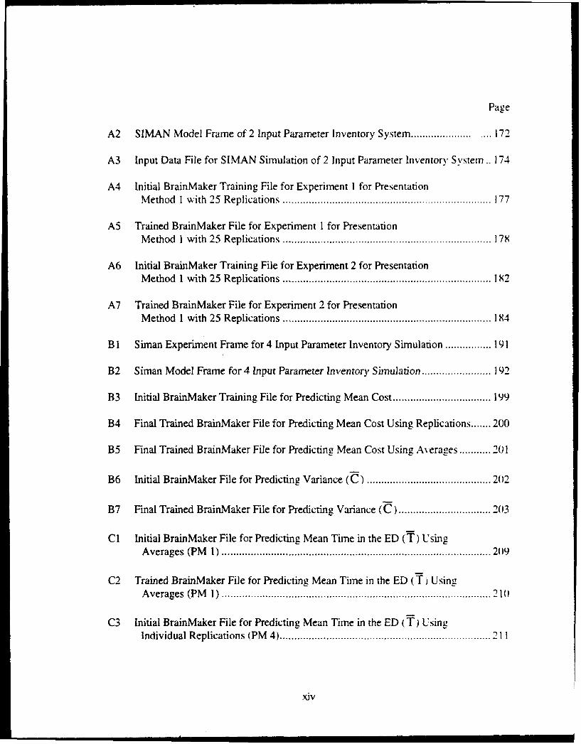
A2 SIMAN Model Frame of 2 Input Parameter Inventory System ........................ 172
A3 Input Data File for SIMAN Simulation of 2 Input Parameter Inventory System .. 174
A4 Initial BrainMaker Training File for Experiment 1 for PresentationM ethod I w ith 25 R eplications ........................................................................ 177
A5 Trained BrainMaker File for Experiment 1 for PresentationM ethod I with 25 Replications .................................................................... 17X
A6 Initial BrainMaker Training File for Experiment 2 for PresentationM ethod I with 25 Replications .................................................................... 182
A7 Trained BrainMaker File for Experiment 2 for PresentationM ethod 1 with 25 Replications .................................................................... 184
B 1 Siman Experiment Frame for 4 Input Parameter Inventory Simulation ................ 191
B2 Siman Model Frame for 4 Input Parameter Inventory Simulation ........................ 192
B3 Initial BrainMaker Training File for Predicting Mean Cost .................................. 199
B4 Final Trained BrainMaker File for Predicting Mean Cost Using Replications ....... 200
B5 Final Trained BrainMaker File for Predicting Mean Cost Using Averages ..... 2()1
B6 Initial BrainMaker File for Predicting Variance (C) ........................................... 202
B7 Final Trained BrainMaker File for Predicting Variance (C) ............................. -03
C1 Initial BrainMaker File for Predicting Mean Time in the ED (T) UsingA verages (PM 1) ........................................................................................ 2()9
C2 Trained BrainMaker File for Predicting Mean Time in the ED (T1 UsingIA verages (PM 1) ........................................................................................ 21(1
C3 Initial BrainMaker File for Predicting Mean Time in the ED (T LUsingIndividual R eplications (PM 4) ......................................................................... 211
Xiv

Page
C4 Trained BrainMaker File for Predicting Mean Time in the ED (T LUsingIndividual Replications IPM 4) ........................................................................ .212
C5 Initial BrainMaker File for Predicting Variance of Mean Time in the ED ............. 213
C6 Trained BrainMaker File for Predicting Variance of Mean Time in the ED ......... 215
xv
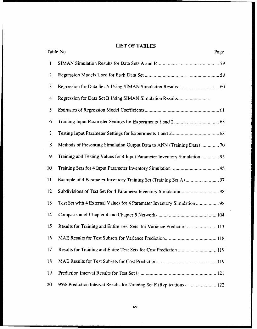
LIST OF TABLES
Table No. Page
I SIMAN Simulation Results for Data Sets A and B ........................................... 59
2 Regression Models Used for Each Data Set ................................................... 59
3 Regression for Data Set A Using SIMAN Simulation Results .............. 6...... 0
4 Regression for Data Set B Using SIMAN Simulation Results ..........................
5 Estimates of Regression Model Coefficients .................................................... 61
6 Training Input Parameter Settings for Experiments 1 and 2 .............................. 68
7 Testing Input Parameter Settings for Experiments 1 and 2 ................................. 68
8 Methods of Presenting Simulation Output Data to ANN (Training Data) ....... 70
9 Training and Testing Values for 4 Input Parameter Inventory Simulation ....... 95
10 Training Sets for 4 Input Parameter Inventory Simulation ............................... 95
11 Example of 4 Parameter Inventory Training Set (Training Set A) ..................... 97
12 Subdivisions of Test Set for 4 Parameter Inventory Simulation .............................. 98
13 Test Set with 4 External Values for 4 Parameter Inventory Simulation ............. 98
14 Comparison of Chapter 4 and Chapter 5 Networks ............................................. 104
15 Results for Training and Entire Test Sets for Variance Prediction ....................... 117
16 MAE Results for Test Subsets for Variance Prediction ................................... 118
17 Results for Training and Entire Test Sets for Cost Prediction .............................. 119
18 M AE Results for Test Subsets for Cost Prediction .............................................. 119
19 Prediction Interval Results for Test Set 0 ............................................................ I2
20 95% Prediction Interval Results for Training Set F (Replications) ....................... 122
xvi
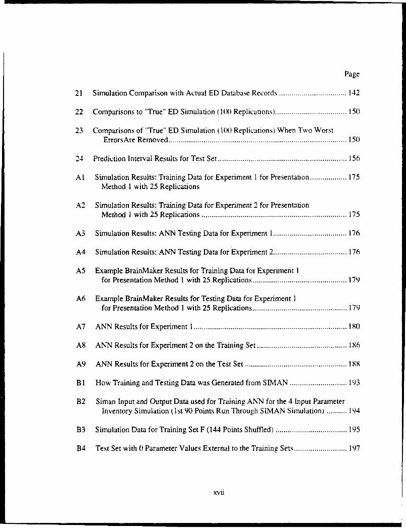
Page
21 Simulation Comparison with Actual ED Database Records ................................. 142
22 Comparisons to "True" ED Simulation (10X) Replications) ................................... 150
23 Comparisons of "True" ED Simulation (100 Replications) When Two WorstErrorsA re Rem oved .................................................................................. 150
24 Prediction Interval Results for Test Set ............................................................... 156
Al Simulation Results: Training Data for Experiment 1 for Presentation .................. 175Method I with 25 Replications
A2 Simulation Results: Training Data for Experiment 2 for PresentationM ethod I with 25 Replications ....................................................................... 175
A3 Simulation Results: ANN Testing Data for Experiment 1 .................................... 176
A4 Simulation Results: ANN Testing Data for Experiment 2 .................................... 176
A5 Example BrainMaker Results for Training Data for Experiment Ifor Presentation Method 1 with 25 Replications .............................................. 179
A6 Example BrainMaker Results for Testing Data for Experiment Ifor Presentation Method I with 25 Replications .............................................. 179
A7 ANN Results for Experim ent I ........................................................................... 180
A8 ANN Results for Experiment 2 on the Training Set ............................................ 186
A9 ANN Results for Experiment 2 on the Test Set .............................................. 188
B 1 How Training and Testing Data was Generated from SIIAN ............................ 193
B2 Siman Input and Output Data used for Training ANN for the 4 Input ParameterInventory Simulation (1st 90 Points Run Through S [MAN Simulation) .......... 194
B3 Simulation Data for Training Set F (144 Points Shuffled) ................................... 195
B4 Test Set with 0 Parameter Values External to the Training Sets .......................... 197
xvii

Page
Cl ANN Training Data for Emergency Department Simulation ............... 5.... 205
C2 ANN Testing Data for Emergency Department Simulation ................................. 207
C3 ANN Test Set Results for Mean Time in the ED (T) .............................................. 217
C4 ANN Test Set Results for Variance of Mean Time in ED (VarT j ....................... 219
xviii
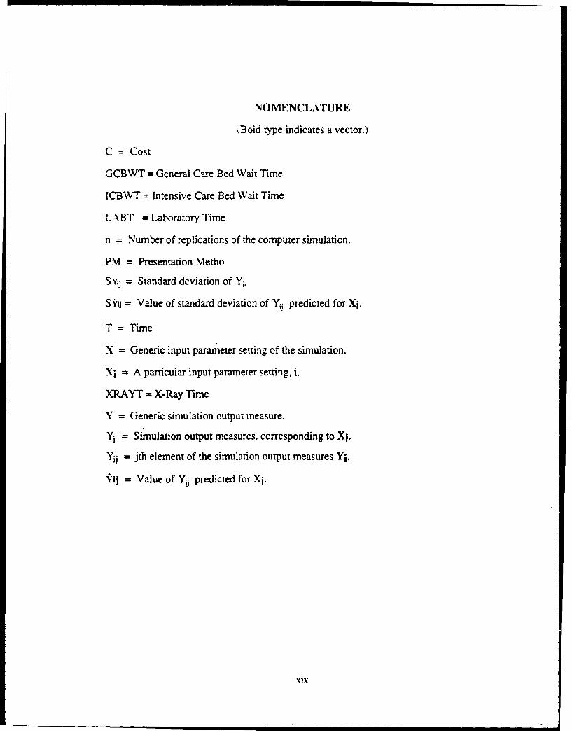
NOMENCLATURE
i Bold type indicates a vector.)
C = Cost
GCBWT = General Care Bed Wait Time
ICBWT = Intensive Care Bed Wait Time
LABT = Laboratory Time
n = Number of replications of the computer simulation.
PM = Presentation Metho
S Y1j = Standard deviation of Yi.
S i'u = Value of standard deviation of Y1j predicted for Xi.
T = Time
X = Generic input parameter setting of the simulation.
Xi = A particular input parameter setting, i.
XRAYT = X-Ray Time
Y = Generic simulation output measure.
Y= Simulation output measures. corresponding to Xi.
Yij jth element of the simulation output measures Yi.
iij = Value of Yij predicted for Xi.
.Nix

1.0 INTRO)DUCTIO)N
1.1 Problem Statement
The interactions and relationships among components of most real world systems
are too numerous and complex for a human to recognize, much less understand. Thus.
simplifications or approximations of systems, called models, are used to examine problems
associated with the design, operation, maintenance, or modification of systems. Many of
these models are implemented as computer simulations that accurately reflect much of the
detailed interactions and activities of the components of the system. Essentially these
computer simulations are mechanisms for converting system input parameters into output
measures.(1)*
According to Box and Draper, there are two basic approaches to building a model
of a system: mechanistic and empirical.( 2) In the mechanistic approach, enough is known
about the system to develop an explicit representation that tries to mimic its operation or
processes. When the necessary information of the physical mechanism of the system is not
known, then an empirical model that relies only on the observations of the inputs and
outputs of the system can be constructed if there is enough observational data on the real
system. For large, complex systems it is usually necessary to combine both approaches in
order to realistically model the system. The development and use of both types of
modeling approaches are depicted in Figure 1. As can be seen in Figure 1, the main
difference between the two approaches is in the creation or development of the model,
rather than the operation of the completed models.
*Parenthetical references placed superior to the line of text refer to the bibliography.

2
Development of the model.F:>@MCAISTIC MDL
Ei '---MOELOUTPUT
*$4$TMI M EM ICAL ~ fSYSTEM OUTPUT }JOIDDE N=110ý OUTPU
USED WHEN OPERATING THE MODEL
Figure 1 Mechanistic and Empirical Modeling Approaches
Mechanistic models are generally preferred over empirical models because of the
clear and apparent connections to the real system. However, a major drawback to many
mechanistic models is that they can be extremely slow to operate, thus requiring
tremendous amounts of computer resources.
Consider a fairly common situation where a slow but accurate mechanistic
computer simulation model of the system exists and there is very litt!e observational data
of the real system. One approach to resolving this situation would be to build an empirical
model using the data from the real system. However the lack of real system data would
probably produce a poor empirical model. Another approach would be to take advantage
of the existing mechanistic computer simulation to obtain data for use in developing an
accurate and fast operating empirical model. In this approach the empirical model is
actually a metamodel (i.e., a model of the computer simulation model), rather than a direct
model of the system.

3
For more than twenty years, metamodels based primarily on response surface
techniques, have been used to examine computer simulations. Most response surface
methods currently use linear regression to build empirical models of computer
simulations.(3 ) The central idea of this research is to use Artificial Neural Networks
(ANN) to construct the empirical model of the computer simulation, since ANN are
essentially capable of performing non-parametric, nonlinear regression.( 4) Figure 2
shows the metamodeling approach and tenninology for the regression and ANN empirical
models.
First, obtain simulation data ...
Input MECHANISTICCOMPUTER OutputSIMULATION Otu
then, develop an empirical model using observed simulation data.
Simulation IndependentInput = Variable EMPIRICAL
REGRESSION Predicted Value
Simulation Dependent MODELOutput = Variable
Simulation siuuInput StimulusEMPIRICAL
ANN ResponseSimulation MODEL
Output - Target
Figure 2 Constructing Metamodels of Computer Simulations
While beyond the scope of this dissertation, the ultimate goal is to use ANN
approximations in lieu of mechanistic computer simulations in performing such complex
and time consuming advanced tasks as simulation 'optimization,' sensitivity analysis, and
simulation aggregation/reduction. In order to attain this goal, it is necessary to study and
4
understand the limitations and strengths of ANN approximations to perform the most
elementary, yet fundamental, tasks of simulation. Computer simulations are used to
perform the following basic tasks:
To predict the output measure of a system for a given input parameter setting.
To determine the output measure's average value and variance for a given inputparameter setting.
To determine if the output measure for a given input parameter setting issignificantly different than a specified value of interest to a decision maker.
To determine sensitivity of the output measure to change in the input parameters.
The problem that this dissertation addresses is how to perform these basic
simulation tasks with ANN approximations of a computer simulation rather than
performing these tasks directly with the computer simulation. This dissertation provides
the foundation for using ANN approximations of a computer simulation to perform
advanced simulation tasks.
1.2 Importance of Computer Simulation
Computer simulation has been identified in surveys as the most widely used tool of
industrial engineers and management scientists.( 5) Computer simulation has several
advantages over other techniques for examining systems. Often computer simulation is
the only means for examining a real world system. Sometimes, this is due to the size and
complexity of the system, since some systems cannot be accurately represented by an
analytical mathematical model. On other occasions, this is due to the fact that the system
does not exist or the conditions under which the system will operate are too dangerous,

costly or infrequent to permit direct experimentation with the system. Examples include
the United States space station, conducting nuclear war, and designing the tunnel under
the English Channel between England and France. Other advantages of simulation include
the ability to have complete control over the experimental conditions and to study system
operation over long time horizons.Y6•
There are a wide variety of application areas such as the military, service
industries, manufacturing organizations, and transportation companies throughout the
world that make extensive use of computer simulations. For example in the military,
computer simulations are used to conduct training for individual soldiers in tanks and
aircraft, examine operation plans and force structures, as well as to evaluate future
weapons systems.(7 ) The main reason these computer simulations are being used is that
they provide realistic results and, in many cases, provide them at a lower cost than
alternative approaches.
1.3 Problems with Computer Simulations
Simulation models often are expensive to develop and use, in terms of personnel,
time, and other resources. Sometimes too much confidence is placed on the results of a
computer simulation simply because these results were produced by a large, very detailed
computer program. Computer simulation models also have the opposite type of problem:
the results are not accepted because decision makers consider the large, detailed computer
program to be a 'black box.' Additionally proper interpretation of computer simulation
output usually requires training and experience in using statistical methods to prevent

6
people from doing such things as interpreting the results of one replication of a stochastic,
simulation as being 'the answer.'("'
Simulation is typically considered a 'means of last resort' due to the cost of
building, verifying, validating, and using simulation models. Hillier and Lieberman
succinctly state: "... simulation is a slow and costly way to study a problerm", 9M The longer
it takes to run a computer simulation on a particular computer platform, the more difficult
it is to perform the necessary checks involved with verifying and validating the cornputcr
simulation. Another problem is that these simulations can grow so large theit they exceed
the memory capacity of the computers, or the commercial modeling languages, that are
available to the users of the simulation. Even after expending the resources to obtain a
valid model, slow response time or large memory requirements, caused by the complexity
of the computer simulation, can prevent, or seriously impede, such activities as perforling
quick turn-around studies, sensitivity analyses, model aggregation, and simulation
'cptimization'.
1.4 Need for Better Approximations to Computer Simulation Models
For more than 30 years, computer simulation models have been used to predict
how systems would perform under certain conditions. Many of these models have been
accepted as valid representations of the underlying system because the model accurately
reflects the behavior of the systern as it operates over time. Over the past several years. in
combination with response surface methods, these models have also been used, not only to
predict the behavior of a system for a given set of input parameters, but also to prescribe

7
the input parameter settings that would result in good or 'optimal' output values of the
model with respect to the particular problem of concern.
However, because of the detailed information that is necessary for precise
prediction over time, it is difficult to find 'optimal' solutions to these predictive models.
What makes it so difficult to 'optimize' a predictive model is that they are usually
computationally expensive and have a very large number of possible solutions in the input
parameter space. In 1989, Jacobson and Schruben state that "Although there has been a
significant amount of research in the area (simulation optimization), no general approach
has been developed into an efficient and practical algorithm."0 0) This situation still holds
five years later. Thus, there is a need to reduce the computational burden of computer
simulations to permit identification of good solutions for designing, operating, and
maintaining large, complex systems.
Typically, computer simulation 'optimization' is currently conducted through
response surface methodologies (RSM) using regression model approximations of the
computer simulation. The regression model approach in RSM has been used successfully
for such purposes as performing sensitivity analyses within a limited region of the input
parameter space, determining constraint satisfying solutions, and simulation
,optimization'.(' 1) The regression model approach has not been used to perform global
estimation or approximation. The regression model approach has typically been limited to
fist- and second-order regression models.(02) Myers, Khuri and Carter state: "There
appears to be some need for the development of non-parametric techniques in RSM.
Most of our analytic procedures depend on a model. The use of model-free techniques

would avoid the assumption of model accuracy or low-order polynomial approximations
and, in particular, the inposed symmetry associated with a second-degree polynomial."(13)
The possible approaches to solving the problems caused by the computational
burdens of computer simulations are to obtain more powerful hardware, rewrite the
computer simulation to be more computationally efficient, or to develop a small and/or
fast approximation to the computer simulation. In many cases, the first and second
approaches have already been taken or were impractical due to a lack of capital funds or
the ability of available simulation programmers. In addition, if a computer simulation has
achieved a high degree of user acceptance due to extensive verification and validation
efforts, there is a certain amount of reluctance to make significant modifications to the
computer simulation. Thus, the third approach, approximating computer simulations,
needs to be examined.
As Simon puts it, "When our goal is prescription rather than prediction, then
we can no longer take it for granted that what we want to compute are time series ...
But facts must be faced. Intelligent approximation, not brute force computation is still
the key to effective modelling. ,(14)
1.5 Using ANN to Approximate Computer Simulations
One possible non-parametric approach, which is the focus of this research, is to
have an artificial neural network "learn what the computer simulation knows" by training
on the inputs and outputs of the computer simulation. As Padgett and Roppel state:
"Neural networks in all categories address the need for rapid computation, robustness, and

9
adaptability. Neural models require fewer assumptions and less precise information about
the systems modeled than do some more traditional techniques."('15)
The idea of using an ANN to approximate a computer simulation may initially
seem routine to researchers with an extensive background in neural networks. The reason
for such an assessment is that there are many examples of researchers using computer
simulations in order to obtain data to train their networks.(0 6.17,s1 ) The majority of these
cases involved research in modifying or developing new ANN methodologies, techniques,
or procedures. Thus, instead of expending valuable time and effort to obtain data from a
real system, these researchers obtained their data from computer simulations that were
built with the sole purpose of "feeding" an ANN. However, while it might be fairly trivial
to build a computer simulation to provide training data to an existing ANN, this does not
mean that it will be easy to build an ANN that will be able to receive and learn the
relationships of an existing, complex stochastic computer simulation.
ANN have been used quite extensively to perform function approximation.
However, computer simulations of the type examined in this dissertation are more difficult
to approximate. There are three major differences between using ANN to approximate
stochastic simulations and using ANN to perform ordinary function approximation. First,
due to the stochastic nature of the computer simulation, a given set of inputs yields
different outputs, thus compounding training. Second, training and testing data are
computationally expensive to generate, and therefore must be leveraged. Third, training
and testing data are usually designed; i.e., are not randomly chosen from the problem
domain.( 19 )
l()
While the largest payoffs for a computer simulation approximation tool are likely
to be in the complex areas of simulation optimization, sensitivity analysis, and model
aggregation, it is necessary that a solid foundation be established for using the
approximation tool, either in lieu of, or in conjunction with, the computer simulation.
Therefore, it is essential to know how to use the approximation tool to perform the most
rudimentary computer simulation tasks.
The major contribution of this dissertation is that it provides an empirically based
methodology and discusses the capabilities, limitations, advantages and disadvantages, for
using ANN approximations of computer simulations to perform the basic simulation tasks
of prediction and comparison of alternatives. An additional contribution is the
development of the foundation for using ANN approximations of computer simulations for
performing advanced simulation tasks.
1.6 Overview of the Dissertation
This dissertation contains eight chapters and three appendices. Chapter I provides
a general introduction to the problem of approximating computer simulations with
Artificial Neural Networks. A detailed literature review of computer simulation,
approximation theory, and approximation approaches is given in Chapter 2. The research
issues, methodology and tools used to conduct the research are detailed in Chapter 3.
Chapters 4 and 5 cover the description, experiments, results and lessons learned from the
problem used to develop the baseline Artificial Neural Network metamodel approach.
Chapter 6 delineates the baseline ANN metamodel approach. Chapter 7 provides the
results of applying the baseline ANN metamodel approach on a demonstration problem,

specifically a simulation of an emergency departnent. Chapter 8 contains the summary
and conclusions derived from the research effort as well as areas for potential future
research. The appendices and bibliography follow Chapter 8.
1.7 Restrictions of the Research
Since the focus of this research effort is on developing a tool that could be used to
approximate a computer simulation, it is assumed that the topology of the internal
relationships and procedures within the computer simulation have been determined and
will not be modified (i.e., the computer simulation to be approximated has already been
finalized, verified, and validated). Therefore, this research did not address problems
associated with building computer simulation models. Nor does it deal in detail with
problems of verification and validation of computer simulation models. Further, it is
assumed that only the values of the input parameters that are provided to the computer
ýsmulation can be changed.
The prediction of output values will only be done for those output values
determined at the termination of the simulation. Predicting a series of values of the output
measure over time is a subject for future research efforts.
This research only examined terminating, stochastic, discrete-event computer
simulations. A description of these terms is provided in Chapter 2. This research focused
on the type of computer simulation typically used for addressing industrial
engineering/management science/systems analysis problems. However, this same
approach should be generalizable to other areas.

12
This research uses feedforward, multi-layered, fully connected artificial neural
networks trained via the backpropagation learning algorithm. The reasons for having
chosen such a network paradigm are discussed in Chapter 3.
1.8 Summary
This chapter provides an introduction to the problem of interest. Specifically, it
presents an overview and demonstrates the need for approximating computer simulations
with artificial neural networks. A brief discussion of the topics of computer simulation
and its importancc, modeling approaches, and the fundamental idea of using the results of
a computer simulation to provide data for building an empirical model of a system are
also provided. An overview of the dissertation document is provided as well as a
discussion of the restrictions of the research effort.

13
2.0 LITERATURE REVIEW
2.1 Computer Simulation
Simulation has been defined by Pegden as: "the process of designing a model of a
real system and conducting experiments with this model for the purpose of understanding
the behavior of the system and/or evaluating various strategies for the operation of the
system."( 20 ) Just about anything can be simulated on a computer. Computer simulations
range from models of simple mathematical functions, such as y = sin(x)+4x, to complex
models of the universe.
There are various ways that computer simulations can be classified. Law and
Kelton provide a way to categorize computer simulations using four dichotomous
characteristics:(2 1)
(1) Deterministic versus Stochastic. Deterministic simulations provide a unique
solution for a given input, no matter how many replications are performed, whereas the
stochastic simulation contains probabilistic elements, and therefore provides only an
estimate of the output variable.
(2) Static versus Dynamic. A static simulation is a representation of a system
where time does not have an impact, while a dynamic simulation is affected by the passage
of time within the simulation.

14
(3) Discrete versus Continuous, or Mixed. This is a characteristic of dynamic
computer simulations. In discrete simulations, the variables can change only at specific
points (at most a countably infinite number of points) in time, whereas in continuous
simulations, the variables change continuously (i.e., without a break or jump between
values) over time. A mixed simulation contains some variables which are discrete and
some which are continuous.
(4) Terminating versus Non-terminating. This is a characteristic of dynamic
computer simulations. A terminating simulation is one where there exists a natural
termination criteria for the system that is being simulated. A non-terminating simulation
does not have a natural termination criteria and so analytical or heuristic methods are used
to determine when to stop the simulation.
To a great extent the answer to the question "what is computer simulation?"
depends on the respondent. Each area of specialization such as aeronautics, chemistry,
economics, nuclear engineering, medicine, physics, or warfare has its own repertoire of
computer simulation models that are used in research and applications. Due to the
characteristics of the problems in each area, certain types of models will perform better
than others and will, therefore, tend to dominate a field of specialization. For instance, in
the fields of operations research, systems analysis, and industrial engineering, which
developed concurrently with the use of computers, Quade states "... simulation is the
process of representing item by item and step by step the essential features of whatever it
is we are interested in... ,"(22) Thus, researchers in these fields tend to think of computer
simulations as mechanistic models of systems. In this dissertation it is assumed that the
term computer simulation means a mechanistic, stochastic, dynamic, discrete, terminating

15
simulation since the majority of simulations in the field of industrial engineering are of this
type. Discrete-event models are by implication dynamic as well as discrete. Thus, this
research considers mechanistic, discrete-event, stochastic, terminating computer
simulations.
In the past, many organizations had the luxury of making decisions on the basis of
studies of long duration, and thus, the computer simulation models that were used in
conducting these long duration studies did not need to be very fast. This situation was
especially pronounced for examinations of very large and complex systems such as rain
forests, space stations, and military operations. Today, with more managers becoming
comfortable with the use of computers and computer simulation models, as well as the
increasing pressures of global competition, there is a greater demand to have results from
computer simulations in a shorter amount of time.(23-28) If the computer simulation is too
slow, as can typically be the case when portions of the simulation employ large Monte
Carlo modules to generate responses, then the results may not be available in time to assist
the decision maker.
Computer simulations are also used to perform sensitivity analysis for large
complex systems.(29) Sensitivity analysis means being able to answer the "what if'
questions that a decision maker might ask concerning the issues that are being
investigated. This typically requires making many different runs and replications of each
variation of the input parameter settings. Thus, if the computer simulation is slow, the
amount of sensitivity analysis that can be performed will be limited. Sensitivity analysis of
computer simulations currently can be very expensive.(6)

16
Computer simulation models for very large, complex systems are sometimes
constructed by building a series of models for different system components, usually called
modules, and then linking them together to form an aggregate model of the system. While
each of the individual modules might perform quite effectively, the aggregate model might
be very slow and possibly exceed the memory requirements of the computer. Thus, there
is a need for model reduction techniques to make the larger and more computationally
expensive modules more efficient.(30, 31)
Over the past several years, computer simulation models have also been used, not
only to predict the behavior of a system for a given set of input parameters, but also to
prescribe the input parameter settings that would result in "optimal" output values of the
model with respect to the particular problem of concem.( 32) It should be noted that what
is meant by an "optimal" solution in the context of simulation is really closer to a
"superior" solution rather than the "best" solution interpretation typically found in the field
of optimization. However, because of all the detailed information necessary for precise
prediction over time, it is difficult to find optimal solutions to these models. Just as
humans become overloaded with information about the real world when it is necessary to
predict the behavior of such systems, these computer simulation models may be processing
too much irrelevant information when it comes to prescribing solutions to posed problems.
2.2 Artificial Neural Networks
A neural network is a computational mechanism that achieves power and flexibility
through the use of parallel and sequential processing elements. The field of neural
networks is also known as parallel distributed processing or connectionism.(33) The initial

17
focus of neural networks was, and the work of many current researchers is, on developing
artificial structures that model the actual operation of a biological brain. Many other
research efforts, including this one, make no claims about their neural networks reflecting
features of how the brain actually operates. To emphasize the distinction, the latter group
of networks are referred to as artificial neural networks (ANN).
The earliest work in neural networks was reported in 1943 by McCulloch and Pitts
who developed networks which today are called "McCulloch-Pitts nets." While these nets
are very simple by current standards, the noted mathematician John von Neumann proved
that redundant McCulloch-Pitts nets can perform arithmetic calculations with high
reliability, but not necessarily as efficiently as traditional sequential computing
algorithms.(34) Currently, there are many different kinds of neural networks with various
architectures and learning algorithms that are used for many different purposes in a wide
variety of applications.(35,36) Cheng and Titterington provide an excellent discussion of
neural networks from a statistical perspective by examining the similarities and differences
between traditional statistics and artificial neural networks.( 37)
It should be noted that in the field of neural networks the term "computer
simulation" has typically been used in two different ways. The more prevalent use is to
indicate a software implementation of an ANN on a sequential processing computer to
distinguish it from a hardware implementation on a parallel processing computer or
chip.(38) A secondary use is to describe one of the mechanisms for obtaining data to test
an ANN methodology, technique, or structure. This is typically done when it is difficult or
impossible to obtain real world data. This secondary interpretation is closer to the manner
in which the term "computer simulation" is used in this research.
Is
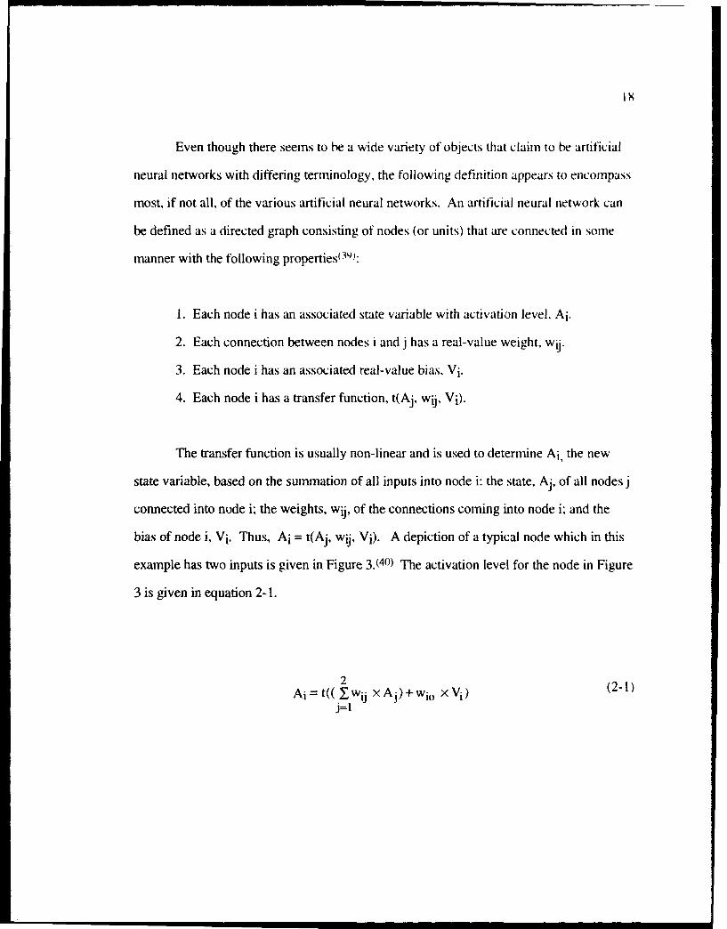
Even though there seems to be a wide variety of objects that claim to be artificial
neural networks with differing terminology, the following definition appears to encompass
most, if not all, of the various artificial neural networks. An artificial neural network can
be defined as a directed graph consisting of nodes (or units) that are connected in some
manner with the following properties( 39):
1. Each node i has an associated state variable with activation level, Ai.
2. Each connection between nodes i and j has a real-value weight, wij.
3. Each node i has an associated real-value bias, Vi.
4. Each node i has a transfer function, t(Aj, wij, Vi).
The transfer function is usually non-linear and is used to determine Ai, the new
state variable, based on the summation of all inputs into node i: the state, Aj, of all nodes j
connected into node i; the weights, wij, of the connections coming into node i; and the
bias of node i, Vi. Thus, Ai = t(AJ, wij, Vi). A depiction of a typical node which in this
example has two inputs is given in Figure 3.(40) The activation level for the node in Figure
3 is given in equation 2-1.
2
Ai WtY( wij xAj)+Wio ×Vi)(-j=l

I I )
19
A,
input 2 Node iFigure 3 A Typical ANN Node
While there is very little that an individual node can do, by combining many
different nodes, ANN are capable of approximating complex functions. The nodes of an
ANN are typically placed into one of three types of layers. The input layer only receives
stimuli or information from outside the network. The output layer is used to provide
results from the network. The hidden layer(s) is used to permit different operations to be
performed on the data. The hidden layer derives its name from the fact that it is invisible
to the world outside of the network. In other words, the hidden layer neither receives nor
transmits any information directly outside of the network. Some types of ANN do not
use a hidden layer of nodes. If, for all layers of the network, all the nodes in one layer of
the network are connected to all the nodes in the succeeding layer of the network, then the
network is called a fully connected neural network. Following the convention used in
Zurada, only the hidden and output layers are counted when describing the number of
layers in the network.(41) For example, a network with an input layer, two hidden layers
and an output layer would be referred to as a three layer network.
One way to characterize networks that are organized into layers is with regard to
the direction of the flow of information between the layers of the network. If the flow of
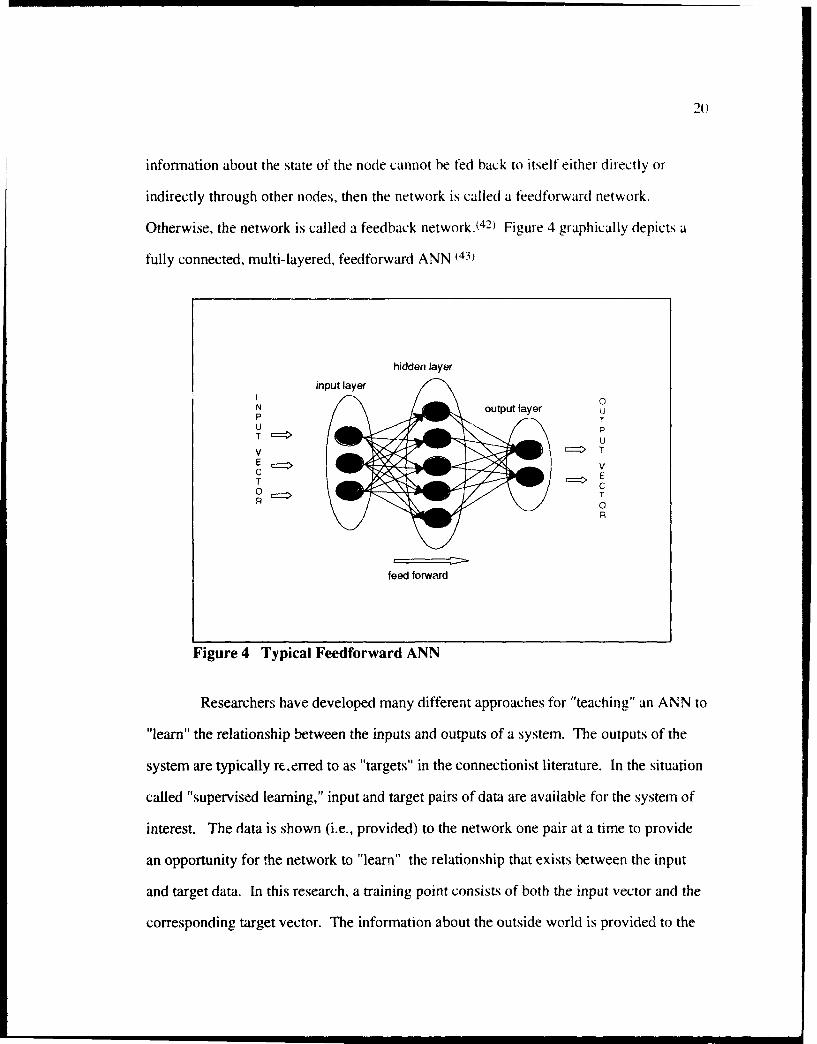
201
infortnation about the state of the node cannot be fed back to itself either directly or
indirectly through other nodes, then the network is called a feedforward network.
Otherwise, the network is called a feedback network 242) Figure 4 graphically depicts a
fully connected, multi-layered, feedforward ANN (43)
hidden layer
input layerI 0N output layer uP TU PT = U
V E TE Vc E
T C0Z TR 0
R
feed forward
Figure 4 Typical Feedforward ANN
Researchers have developed many different approaches for "teaching" an ANN to
"learn" the relationship between the inputs and outputs of a system. The outputs of the
system are typically re.erred to as "targets" in the connectionist literature. In the situation
called "supervised learning," input and target pairs of data are available for the system of
interest. The data is shown (i.e., provided) to the network one pair at a time to provide
an opportunity for the network to "learn" the relationship that exists between the input
and target data. In this research, a training point consists of both the input vector and the
corresponding target vector. The information about the outside world is provided to the

21
ANN through the activation values of the input and output nodes (i.e., through the Ai).
The knowledge of the network is stored in the weights of the network (i.e., in the wij).
Typically, a network starts in a randomized state of initial weights and is trained iteratively
until reaching an "intelligent" state.
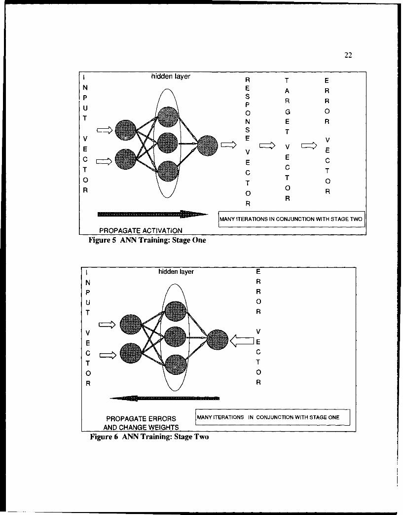
A very popular, nearly "standard", training mechanism is called "backpropagation"
or the "generalized delta rule." First developed by Werbos(44) and publicized widely by
Rumelhart and McClelland,(45) the generalized delta rule is usually used for feedforward,
fully-connected networks and is divided into two stages. In the first stage of training, as is
depicted in Figure 5, one input data vector is presented to the input nodes of the network,
and processed in a forward direction through the network with the states of the nodes
being passed from one node to the next until the output nodes have newly assigned state
values or activation levels, called the response vector. The response values of the output
nodes are then subtracted from the corresponding target values, resulting in an error value
associated with each output node.
The second stage of training, depicted in Figure 6, propagates the squared error
from each output node backwards through the network, and adjustments are made to the
weights and thresholds of the network using gradient descent to reduce the size of the
total squared error of the network.(45) Selecting a new training point and applying both
training stages to the new training point continues until the training stoppage criteria is
achieved. Typical training stoppage criteria include convergence for all of the training
data to less than a pre-specified error level or after performing a pre-deterinined, large
number iterations through the training data.
22
hidden layer R T E
N E A Rp SR RU P
U 0 G 0
N E R
S TV : V V
V E vCE v Ec E E cT c C T
0 T T 0R 0 0 R
RR
"MANY ITERATIONS IN CONJUNCTION WITH STAGE TWO
PROPAGATE ACTIVATIONFigure 5 ANN Training: Stage One
I hidden layer E
N Rp R
U 0
T R
v V
E E
C CT T
O 0R R
PROPAGATE ERRORS MANY ITERATIONS IN CONJUNCTION WITH STAGE ONE
AND CHANGE WEIGHTSFigure 6 ANN Training: Stage Two

23
Once the training is concluded, a check on the generalizability of the trained ANN
is usually performed by testing another set of data, distinct from the training set, using th".
weights determined by the training procedure. This test is conducted in the exact same
way as the first stage of training, but consists of only one pass through the network, as
depicted in Figure 7. The input data is provided to the network and the activations are
propagated only one time for each input data vector and the resulting response is
compared to the target to obtain the error of the ANN on each test point.
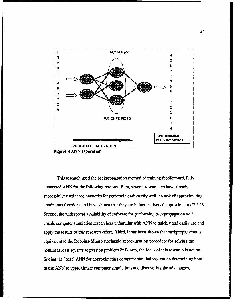
Finally, as is depicted in Figure 8, the trained network is used in an operational
mode to obtain predicted responses to input vectors for which target vectors are not
available. This is similar to testing the network in that there is only one pass for each
point in the data set. However, in this case there are no target vectors to use to determine
the accuracy of the ANN.
hidden layer R TE A E
N S RpP R R
U 0 G 0T N EST
S~E
V V V
E V E E
C E C C
T T T T
0 0 0 0
R R R R
WEIGHTS FIXED
ONE ITERATION
PER INPUT VECTOR
PROPAGATE ACTIVATIONFigure 7 ANN Testing
24
hidden layer RNp E
U S
T P
v N
E C-= s
C ET0 V
R EC
WEIGHTS FIXED T0R
ONE ITERATION
PER INPUT VECTOR
PROPAGATE ACTIVATIONFigure 8 ANN Operation
This research used the backpropagation method of training feedforward, fully
connected ANN for the following reasons. First, several researchers have already
successfully used these networks for performing arbitrarily well the task of approximating
continuous functions and have shown that they are in fact "universal approximators."(46-54)
Second, the widespread availability of software for performing backpropagation will
enable computer simulation researchers unfamiliar with ANN to quickly and easily use and
apply the results of this research effort. Third, it has been shown that backpropagation is
equivalent to the Robbins-Munro stochastic approximation procedure for solving the
nonlinear least squares regression problem.(4) Fourth, the focus of this research is not on
finding the "best! ANN for approximating computer simulations, but on determining how
to use ANN to approximate computer simulations and discovering the advantages,

25
disadvantages and limitations of such an approach. Therefore, to emphasize that this is
not a study of ANN methodology, but rather a study of how to use ANN to approximate
"omputer simulations, a well-accepted, conceptually easy to understand, "standard," ANN
.hat may not be the most efficient at continuous function approximation was used.
There are two major drawbacks of the backpropagation algorithm that have caused
researchers to examine alternative training procedures. The first problem is possible
convergence to local minima rather than the global minimum of the error surface and the
second problem is computational expense and the consequent time to train using
backpropagation.( 55) It was once conjectured that backpropagation trained networks
would always converge to the global minimum. It has been shown that this is true in many
practical applications but there are cases when they do converge to local minima because
it is essentially a gradient descent procedure.(56) One of the reasons that backpropagation
is computationally expensive is that the network architecture, in terms of the number of
hidden nodes, is determined on a trial and error basis. Much of the research has been
directed at examining various methodical procedures. One approach used in this research
is to start with the smallest possible network, train that network, add another node to the
network, and repeat the process until performance begins to worsen. This simple
approach and other more sophisticated techniques such as adding or trimming hidden
nodes during training are discussed by Hush and Horne.(57) Other researchers have
developed such modifications to the traditional backpropagation training algorithm as
Quickprop,(58) RPROP,(59) Double BackProp,(6°) and others based on sophisticated non-
linear optimization procedures. (61-65)

26
Other neural network approaches to function approximation have also been
developed. One of the most promising of these alternatives to backpropagation is Radial
Basis Function (RBF) neural networks. Poggio and Girosi have published several articles
on Radial Basis Function artificial neural networks that have the best approximation
property for continuous multivariate function approximation. 5 1.52.66) However, there is
no guarantee that these networks will also have the best approximation property for
discrete multivariate functions. Also the RBF neural networks are not nearly as well
known as the backpropagation neural networks. For these reasons the RBF neural
networks are not examined in this research. They do appear to hold promise especially in
their ability to provide confidence interval estimates for their responses.(67)
This research used networks with two hidden layers even though it has been shown
that one hidden layer networks can approximate any continuous function.( 68 ,69 ) However,
one hidden layer networks may require an infinite number of nodes to be able to
approximate a given function. In contrast, two hidden layer networks do not require the
assumption of the availability of an infinite number of hidden nodes(70 ) and those networks
can solve most real world approximation problems with only the two hidden layers.(71)
According to Padgett and Roppel: "A neural network can be thought of as an
advanced simulation technique incorporating ideas from many fields and capitalizing on
modern-day parallel processing and microelectronics capabilities."(1 5) Since there are
researchers who are examining the use of the neural network techniques for performing
simulation,'(72) it is obvious that issues such as when should the ANN approach be used to
directly perform the simulation and when should the ANN technique be used to

27
approximate another simulation model, will arise. This research will provide information
that will be helpful in addressing these types of issues.
Four examples in the literature have been found where an ANN was constructed
for the purpose of approximating or estimating the results of a computer simulation
model. The first example, by Fishwick, found that a backpropagation trained neural
network was not as effective as a regression model in approximating a deterministic
computer simulation. However, it should be noted that the author appears to have only
trained one network and did not change any of the default settings of the neural network
software package used in the research.(73) In the second example, Pierreval and
Huntsinger examined the issue of whether the data used to train neural networks as
metamodels of computer simulations should be factorial design points or randomly
generated points. While randomly generated points seemed to produce better networks in
terms of generalizability to test set data, it appears that this was due mostly to the fact that
the random training sets were larger than the factorial design training sets.(74 )
In the third example, Badiru and Sieger reported good results when using a neural
network trained on economic models.(75)
In the fourth example, Hurrion showed that "it is possible to fit a neural network
to model the generalized response of parameter changes in a visual interactive
simulation."(76) The simulation was a stochastic, discrete event, terminating model of a
train depot developed as a demonstration of "visual interactive sinulation."( 77) A random
number of trains arrived at the depot each day to receive coal and the depot remained
open until all of the trains had departed the depot. The output from the simulation was the
length of time the depot remained open each day.

28
Hurrion conducted two experiments in approximating the simulation of a coal
depot with a backpropagation trained fully connected feedforward artificial neural
network. The first experiment was designed to show that a simulation could be
approximated by a neural network. Five different input factors were chosen with each
factor having three different levels. The simulation was replicated nine times at each of
the 35 (i.e., 243) design points and the mean and variance, of the time the coal yard
remained open was calculated over the nine replications. The 99% lower and upper
confidence limits for each of the design points were also calculated. Artificial neural
networks were then constructed to try to approximate the simulation results of mean,
lower confidence limit and upper confidence limit of the time the coal yard was open.
The network architecture that was able to learn the relationships between the input factors
and the output responses had five input nodes, one for each of the input factors, thirty
hidden nodes in each of two hidden layers, and three output nodes. The output nodes
corresponded to the mean and the two confidence limits. The result for the training set
was that the neural networks prediction of the mear, always fell within the original
simulation's 99% confidence intervals. in addition, the mean predicted by the neural
network for a test set of six different combinations of input parameters that were not
included in the training set, also fell within the 99% confidence intervals of the original
simulation. The test set was small in comparison to the training set and all of the values
were internal to the values included in the training set. This experiment showed that "it is
possible to fit a neural network to obtain the general response of a simulation's output
over a wide range of input factors."( 78)
Hurrion also demonstrated an incremental approach of building a series of neural
network approximations to a computer simulation, where each neural network

29
approximation was used to guide the selection of future points for simulation and addition
to the training set. One purpose of this demonstration was to show that the neural
network approximation could be used as a tool for facilitating the interaction between the
developer and client of a computer simulation model by providing very quick replies to
"what if" questions posed by the client.(76)
In addition to using ANN to approximate the output of a system for a given set of
input parameter values, some work has demonstrated the potential for using ANN to
performing inverse mappings (i.e., for a given set of system output measures predict the
corresponding system input values).(79-81) In one case, an approach using
backpropagation trained ANN to learn the inverse of the simulation of a manufacturing
facility job shop was demonstrated.( 82) In this example, the simulation had three input
parameters that were varied and four output measures that were generated by the
simulation. The three input parameters were the number of resources in each of three
separate work centers of the job shop. The four output measures were mean tardiness
time, mean flow time, mean resource utilization and workload completion time.
Two neural network architectures were used to learn the inverse of the simulation.
Both neural networks had four input nodes corresponding to the output measures of the
simulation and three output nodes correspcnding to the input parameters for the
simulation. One network had one hidden layer of eight nodes and the other network had
one hidden layer of fifteen nodes. The approach consisted of starting with a small initial
training set of five (output, input) training pairs. Once the network learned the small
training set, the network was used to predict the inputs to the simulation that would
generate a set of desired output measures.

30
The simulation was then run at the predicted input parameter settings to obtain
another observation of simulation output measures. The inputs generated by the ANN and
the new outputs from the simulation were then added to the training set and used to train a
new neural network. This iterative procedure continued until the outputs from the
simulation that used the inputs generated by the ANN matched the desired outputs of the
simulation.
The prelin-dnary results of this example showed that the approach has promise
since both of the networks showed improvement in the output measures of the network-
predicted input parameter settings of the second iteration over the first iteration of the
procedure. As Chryssolouris et at. point out, the procedure of using computer simulations
to provide the data for training artificial neural networks has the potential for reducing the
number of simulations required when using simulation to support manufacturing system
design.(82)
One example was found in the literature in which an artificial neural network was
used to replace a portion of the rule base of a discrete event computer simulation.(83) A
portion of the expert system module of the U. S. Army's Combined Arms and Support
Task Force Evaluation Model (CASTFOREM) was used off-line to train an ANN to make
classification decisions. The decision that the ANN was trained to make was when the
Orange forces should withdraw when being attacked by the Green forces. The inputs to
the ANN were the number of Orange losses, number of Green losses, and the distance
between the two forces. The output of the ANN was a classification of either to withdraw
or not withdraw. The ANN was trained with the backpropagation training procedure and
demonstrated that ANN can be made as reliable as current artificial intelligence symbolic

31
methods. A second type of ANN was added to the model to permit the network to learn
from the experience of the decisions made during the operation of the computer
simulation. The second ANN had the same architecture as the first ANN with the addition
of a goal node and goal sub-nodes. The goal that was used in this example was to
maximize the difference between the Orange losses and the Green losses. An
unsupervised training algorithm was used to permit the network architecture to adapt to
the information provided by additional replications of the computer simulation. An
unsupervised training process does not require a teacher that knows what the outputs
should be for the training inputs. This example demonstrates that artificial neural
networks could be used to develop "adaptive simulations."(84)
A final application of ANN that is of relevance to this dissertation is the use of
neural network! as r- Hlers. Much work has been done using actual system data to
develor neural network controllers on systems as diverse as robots, automobiles, aircraft,
space stations and manufacturing plants.(85-8 7) One group of researchers used neural
networks trained on computer simulations to develop heuristic rules for scheduling a
flexible manufacturing system.(88) One conceptual paper by Wan and Cochran, without
any experimental results, outlines an approach to develop a controller for a system using a
simulation of the system and a neural network approximation to the simulation.(8 9)
2.3 Metamodels
A metamodel is a "model of a model."(90) Blanning first used the term to refer to
models of decision models and discussed computer simulation decision models as
examples where metamodels could be used to perform sensitivity analyses.(91,92) Earlier,

32
Meisel and Collins had used the term "repro-model" to refer to a model of a model and
described repro-modeling as the "process of developing an approximation to. or
condensation of, a complex (sometimes dynamic) computer-based model."''9 -1 It appears
that metamodel has superseded repro-model as the commonly used term for a model of a
model. On the basis of thirty experiments, Friedman and Pressman demonstrated the
usefulness and applicability of metamodels in simulation analysis.(94) Pratt and Mize
discuss a methodology developed for using metamodel of simulations of manufacturing
systems.(95) Yu and Popplewell provide a summary review of the research that has been
done in the field of simulation metamodels.(96)
Some researchers define a metamodel as a "regression model of the actual
simulation model."(97) While it is true that the most popular technique used in
metamodeling simulations is linear regression, there are alternative ways of developing a
model of a model. In particular, this dissertation explores the use of artificial neural
networks as metamodels of computer simulations. Barton discusses the state-of-the-art in
metamodeling and provides an excellent review of several alternative metamodeling
methods. He suggests the following criteria which might prove useful in choosing from
among competing metamodeling techniques:(3)
1. The ability to gain insight from the form of the metamodel.2. The ability to capture the shape of arbitrary smooth functions based on observed
values which may be perturbed by stochastic components with general distributions.3. The ability to characterize the accuracy of fit through confidence intervals, etc.4. The robustness of the prediction away from observed (x,y) pairs.5. The ease of computation of the metamodel.6. The numerical stability of the computations, and consequent robustness of
predictions to small changes in the parameters defining the metamodel.7. The existence of software for computing the metamodel, characterizing its fit,
and using it for prediction.
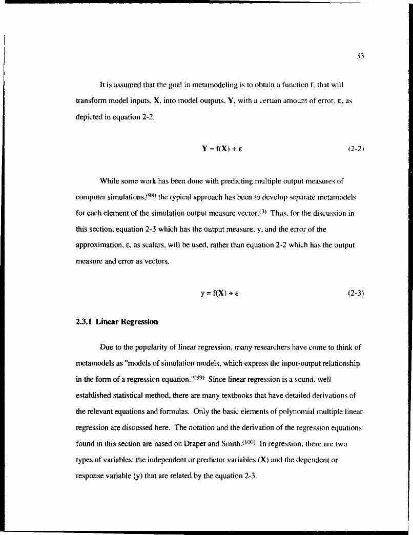
33
It is assumed that the goal in metamodeling is to obtain a function f. that will
transform model inputs, X, into model outputs, Y, with a certain amount of error, F, as
depicted in equation 2-2.
Y = f(X) + F- (2-2)
While some work has been done with predicting multiple output measures of
computer simulations,(9 8) the typical approach has been to develop separate metamodels
for each element of the simulation output measure vector.(3 ) Thus, for the discussion in
this section, equation 2-3 which has the output measure, y, and the error of the
approximation, e, as scalars, will be used, rather than equation 2-2 which has the output
measure and error as vectors.
y = f(X) + E (2-3)
2.3.1 Linear Regression
Due to the popularity of linear regression, many researchers have come to think of
metamodels as "models of simulation models, which express the input-output relationship
in the form of a regression equation."( 99) Since linear regression is a sound, well
established statistical method, there are many textbooks that have detailed derivations of
the relevant equations and formulas. Only the basic elements of polynomial multiple linear
regression are discussed here. The notation and the derivation of the regression equations
found in this section are based on Draper and Smith.(I(MI) In regression, there are two
types of variables: the independent or predictor variables (X) and the dependent or
response variable (y) that are related by the equation 2-3.
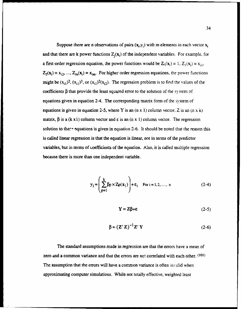
34
Suppose there are n observations of pairs (x,,yi) with m elements in each vector x,
and that there are k power functions Zj(x,) of the independent variables. For example, for
a first-order regression equation, the power functions would be Z,(x) = 1, Z (xi) = xiI,
Z 2(xi) = Xi2, ... , Zm(Xj) = xim. For higher order regression equations, the power functions
might be (xi 1)2, (Xi1 )3 , or (Xi1)2(Xi2 ). The regression problem is to find the values of the
coefficients 13 that provide the least squared error to the solution of the system of
equations given in equation 2-4. The corresponding matrix form of the system of
equations is given in equation 2-5, where Y is an (n x 1) column vector, Z is an (n x k)
matrix, 03 is a (k xl) column vector and E is an (n x 1) column vector. The regression
solution to the."- equations is given in equation 2-6. It should be noted that the reason this
is called linear. regression is that the equation is linear, not in terms of the predictor
variables, but in terms of coefficients of the equation. Also, it is called multiple regression
because there is more than one independent variable.
yi= Zp(xi) +Ei Fori=1,2 ...... n (2-4)
Y = Zj3+E (2-5)
[3=(Z' Z)-1 z" Y (2-6)
The standard assumptions made in regression are that the errors have a mean of
zero and a common variance and that the errors are no+ correlated with each other. (101)
The assumption that the errors will have a common variance is often invalid when
approximating computer simulations. While not totally effective, weighted least

35
squares("° 2) or transformations of the dependent variable(1 113) are sometimes used when the
assumption of common variance cannot be made. Additionally, a typical assumption is
made that the errors are distributed normally with mean of zero and a common variance.
This final assumption permits the construction of confidence intervals for the coefficients
of the model as well as for the predictions of the model. In those cases where normality of
errors cannot be assumed, an alternative approach is to use the generalized linear model
which assumes that the errors come from any family of exponential distributions rather
than restricting them to the normal distribution.
While there are many strengths of polynomial regression models, there are also
some weaknesses. Low-order polynomials have a very limited number of surface shapes
that can be approximated, while high order polynorrials have the tendency for errors to
increase rapidly as the independent variables are mov,-d away from an observation used to
build the regression model.(3)
The field of regression is continuing to grow and expand as evidenced by work in
such areas as nonlinear regression( 4A,10 -5 ) and nonparametric regression.( 1116.107)
2.3.2 Response Surface Methodology (RSM)
Using the term metamodel to mean a "model of a model" is relatively new.
However, the most popular metamodel approach of using low-order linear regression
models in response surface methods (RSM) was formally developed in 1951 by Box and
Wilson to optimize the yield of chemical processes through a series of physical
experiments.(10 8) Since then response surface methods have been extended to include
using regression models to optimize computer simulations. The purpose of RSM is to find

36
the levels of the experimental factors that will yield the best value of the response or
output of a system. The response surface methodology with computer simulation basically
entails a repetitive process of performing the following steps:(5 ())
1. Conduct a set of designed experiments that finds the output response value by
running the computer simulation at various levels of the input parameters for multiple
replications.
2. Approximate the relationship between the input parameters and the output
measures in the current region of interest with a model of the system. Typically. the
approximating models have been first-order regression models.
3. Find a direction in the input parameter space of the model that yields improved
solutions (e.g., in the direction of the gradient, if trying to maximize the response).
4. Move in the direction of improved response and return to Step 1. If there is no
direction of improved response, then develop second-order regression models to obtain a
more accurate characterization of the response surface. Use this second-order regression
equation is to determine if the found region is a locally optimal.
For optimizing computer simulations with single output measures, first-order
regression models are good tools for determining the direction of search in response
surface methods because they can be developed very quickly and it is very easy to
determine the direction of improvement once the model is developed. Although most of
the work in RSM has been with optimizing one dimensional output measures, some work
has been done on optimizing computer simulations with multiple output measures.102)
Improved results have been reported when using different variance reduction techniques

37
such as combining common random numbers and antithetic variates in response surface
methods.(12,11o,11 l)
A good approximation in RSM is needed only in a small region of interest since the
regression models are constantly being replaced as the search for the optimum progresses
across the input space. Hood and Welch provide an excellent description and example of
using RSM with computer simulations.(1 12)
2.3.3 Taguchi Models
Just as with response surface methods, the Taguchi method was not originally
developed to be used with computer simulations, but with physical systems.U 13) Taguchi
developed a very successful method of designing quality into products that was easier to
understand and use by practicing engineers. The Taguchi method using direct physical
experiments is well documented.0 14,1 15) Recently, the Taguchi method has been
successfully used in system design with computer simulation experiments.(1 16-119) At the
core of Taguchi's method is the precept that rather than try to eliminate the sources of
variability in product performance the focus should be on trying to develop products that
are not sensitive to the effects of uncontrolled variation. The Taguchi method uses the
same model as equation 2-4 and assumes the errors of the models have a mean of zero
(i.e., E(Ci) = 0). Instead of assuming that the variance of the errors is a constant however,
it assumed that the variance depends on the value of the independent variables
(i.e., Var(Si) = G2 (Xi)). Taguchi incorporates the information about the variance of the
system by introducing equation 2-7 where the Y is the sample average and the S2 is the
sample variance over the multiple observations at each combination of the independent
variables.

38
10* iog[E(Y2 = Ifpxzp(x) (2-7)p=l
The other variables in equation 2-7 are described in the section on linear
regression. Under Taguchi's approach, it is expected that some independent variables, x,
will have small coefficients of Tp in equation 2-7 and large coefficients of
f in equation 2-5. Those independent variables with small coefficients of gamma are
termed "insensitive to noise." By adjusting the remaining independent variables to
maximize the left side of equation 2-7, the analyst can then set the independent variables
to produce the desired minimimum or maximimum of the response in equation 2-5.(3,12o)
"The Taguchi approach provides an alternative framework to traditional design of
experiments and response surface methods, within which neural network metamodeling
can be used.
2.3.4 Approximation Theory
This established field of mathematics is concerned with problems associated with
approximating continuous, multivariate functions whose values are known at a finite
number of points. This requires determining the values of a fixed number of parameters
W, so that an approximating function, F(X,W), provides the best' approximation or
estimation to the desired function, f(X).(121) Often the approximating function F(X,W) is
a linear combination of basis functions, gi(X), for example F(X,W) = FZaixgi(X), where
the ai are real valued constants. This approach is used in many of the classical methods of
approximating functions including polynomial approximation, spline approximation, kernel
based approximation, and Fourier methods.(122) These and other classical methods suffer
from the need to correctly specify the functional form of the model that will be used in the

39
approximation procedure. In most cases the correct functional form of the model depends
on the data observed from the function. Also, many of the methods assume that the
observed function values are correct (i.e., there is no noise in the data).
The computer simulations examined in this research are stochastic and so they are
not strictly functions. Many of the simulations found in the industrial engineering
literature are of systems with discrete, rather than continuous, input values. In addition, a
linear combination of basis functions can be implemented efficiently via a three layer,
artificial neural network, where each basis function is represented by a node in the hidden
layer of the network.0 23) For these reasons, the approaches used within the field of
approximation theory were not explored further for application to approximating
computer simulations.
2.4 Summary
This chapter provides a survey of the literature concerning the topics involved in
this dissertation. The chapter contains discussion of the broad areas of computer
simulation, metamodels and artificial neural networks each of which are relatively new
fields of research beginning in the 1940s, 1960s and late 1980s, respectively. The history
of each of these fields as well as the definitions of key terms and a review of the literature
relevant to this research are covered. The field of computer simulation is shown to be
quite wide in its scope and applicability to many diverse disciplines. The limitations of
computer simulations for performing studies quickly, sensitivity analyses, and optimization
of systems are delineated. The discussion of artificial neural networks includes a detailed
exposition of the backpropagation training methodology and several examples of other

40
researchers using ANN in conjunction with computer simulations. The discussion of
metamodels includes the history and terminology of metarnodels, regression, response
surface methodology and approximation theory.

41
3.0 RESEARCH METHODOLOGY, ISSUES AND TOOLS
3.1 Methodology of Research
The general research methodology of this dissertation is to develop an approach to
approximating computer simulations using ANN. This is done in two stages. First,
investigating issues through experimentation on a computer simulation of a relatively
simple engineering system. The second stage is to demonstrate the approach on a
computer simulation of a much more complex engineering system. Seven tasks were
defined and are discussed below.
3.1.1 Basic Research Tasks
The first task was to identify the issues that need to be considered for any generic
approach to approximating discrete event, stochastic computer simulations and the
specific issues that might be unique to an artificial neural network (ANN) approach. A
listing of the identified issues is provided in Section 3.2.
The second task was to obtain detailed computer simulation models of two real
world systems that were representative of the types of problems typically examined using
terminating, stochastic, discrete-event computer simulations in the field of industrial
engineering. The first system examined was a relatively simple inventory system. This
system was selected to be able to make comparisons to the problem used in Chapter 12,
"Experimental Design and Optimization" by Law and Kelton.0(14) This system was
analyzed in-depth in order to gain insight into how to approximate a computer simulation
with an ANN model. In this manner, the first system was used as a problem for

42
developing the methodology for approximating computer simulations with ANN. The
description of the system and its computer simulation are presented in Chapter 4. The
second system examined in this research was the emergency deparunent of a large
teaching hospital. This system is representative of large, complex systems and was used as
a research demonstration problem to examine issues of "scale-up" and applicability of the
methodology to, "real world" problems. The description of the system and its computer
simulation are presented in Chapter 7.
The third task was to develop, build, and use simplified representations of the
development problem computer simulation model based on the ANN techniques. A series
of experiments was performed on a two-input parameter version of the inventory system
simulation. These experiments considered various ways of presenting the output of the
simulations to the ANN and predicting multiple outputs. The detailed description and
results of these experiments are also presented in Chapter 4.
The fourth task was to use the ANN approximations of the inve, ,ory system in
place of the original computer simulation model to perform basic computer simulation
tasks of prediction and comparison of alternatives. Part of this task was to compare the
results of the ANN approximation to a second-order multiple linear regression model
approximation. The second-order multiple linear regression model was used for
comparison purposes since it is the highest order regression model typically used in
Response Surface Methods. The final set of experiments used ANN approximations to
make predictions and prediction intervals for the four input parameter inventory system
simulation are discussed in Chapter 5.
43
The fifth task was to develop a methodology for approximating computer
simulations with ANN, based on the results of the experiments on the development
problem. The resulting approach is presented in Chapter 6.
The sixth task was to apply the approach of ANN approximation of computer
simulations to the demonstration problem (i.e., emergency department system). The
results of applying the ANN approximation approach to the demonstration problem are
also provided in Chapter 7.
The final task was to synthesize the lessons learned from performing the basic
simulation tasks with ANN approximations to computer simulations to provide a
framework for using ANN approximations to perform more complex simulation tasks such
as sensitivity analysis, simulation "optimization," and model aggregation/reduction. These
results are discussed in Chapter 8.
3.1.2 Assumptions and Restrictions of the Research
Since the focus of this research effort was to develop a tool that could be used to
approximate a computer simulation, it was assumed that the topology of the internal
relationships and procedures within the computer simulation were determined and would
not be modified (i.e., the computer simulation to be approximated has already been
finalized, verified, and validated). Consequently, this research did not address problems
associated with buildirg computer simulation models. It was assumed that only the values
of the input parameters that were provided to the computer simulation could be changed.

44
The prediction of output values was only done for those values determined at the
end of the simulation. Predicting intermediate results of the output measures over time is
a subject for future research efforts.
This research only examined terminating, stochastic, discrete-event computer
simulations. A description of these terms is provided in Chapter 2. This research focused
on the types of computer simulations typically used for addressing industrial
engineering/managemnent science/systems analysis problems. However, this same
approach could be utilized and should be fruitful in other areas.
Feedforward, multi-layered, fully connected artificial neural networks trained via
the backpropagation learning algorithm were used in this research. Specifically, the basic
backpropagation method popularized by Rumelhart, Hinton and Williams(45) for training
feedforward, fully connected ANN was used for the reasons specified in Chapter 2.
This research used a comprehensive, one-step, experimental design for selecting
the points to be simulated and subsequently used for developing approximations to the
computer simulation. An alternative approach, which was not used in this research, is
sequential experimental design which incorporates information about the responses of the
simulation from preliminary design points to guide the selection of subsequent design
points. The sequential experimental design approach is typically preferred when
conducting computer simulation sensitivity analysis and when using response surface
methods.(025) The work in this research addresses how to do the comprehensive
experimental design and the first step in the sequential experimental design.

45
3.2 Research Issues
The following research questions were identified for consideration and/or experimentation:
How should the simulation output data be presented to the ANN during training'?
How many outputs should be predicted by a single network'?
Can the ANN predict the descriptive statistics commonly used in cornputer
simulations (e.g., mean, variance, minimum, maximum)?
What should the network architecture be for the ANN?
How many different combinations of the input parameters (i.e., experimental
design points) should be used during training?
How many replications of the computer simulation of each combination of the
input parameters should be used during training?
How well does the ANN approximation perform in making predictions of
simulation output measures?
How well does the ANN approximation perform in making prediction intervals of
simulation output measures?
How does an ANN approximation compare with second-order multiple regression
approximations of computer simulations?
3.3 Research Tools
Two commercial products were used extensively in this research:
SIMANXINEMA10 and BrainMakerc. A description of each of these tools and a
discussion as to why they were selected is provided below.

46
3.3.1 SIMAN/CINEMA Simulation Language
SIMAN/CINEMA has been developed by Systems Modeling Corporation of
Sewickley, PA, as a general-purpose simulation modeling language with additional
features that make it very useful for modeling manufacturing systems. The SIMAN
(SIMulation ANalysis) portion of the package is used to create the actual simulation while
the CINEMA portion is used to provide an animation of the simulation.(126 )
A simulation language as opposed to a programming language such as FORTRAN
or Pascal was chosen for use in this research since the majority of work in the simulation
of industrial engineering applications uses higher-level simulation languages.
The SIMAN simulation language was chosen for use in this research for the
following reasons. SIMAN was one of the first major simulation languages available for
use on microcomputers, and it is used extensively in the industrial engineering and
manufacturing fields.(126) SIMAN operates on a wide variety of computer platforms, and
the programs are compatible across the different classes of computers. Hence, S IMAN is
available to many researchers who might be interested in pursuing this research. It is
possible to model almost any kind of system using SIMAN, due to its ability to utilize the
two major approaches used in discrete-event simulation: the event-scheduling approach
and the process interaction approach. SIMAN is relatively easy to use, and has a good
debugging facility. Another reason for selecting SIMAN/CINEMA is the ability to use
CINEMA to animate the simulation for the purpose of verifying and validating computer
simulations. SIMAN also employs Zeigler's theoretical concepts about systems by placing
the system information into two separate component frames of the simulation.( 27) The
physical elements of the system and their interconnections comprise a functional

47
description of the system in a "model" frame. The input parameters and the data
associated with the conditions under which the simulation is to be conducted are placed in
an "experiment" frame.0••)2 This feature greatly assists in performing research experiments
by insuring that changes to the input parameters do not alter the processing steps of the
simulation.
The SIMAN package used in this research was SIMAN IV with runtime processor
version 1.3. The CINEMA package used in this research was CINEMA IV version 1.2.
The simulations were all run on a 486/33mhz personal computer under DOS 5.0.
The SIMAN model and experiment frames for the research development problem
(i.e., the inventory system) are contained in Appendices A and B, respectively.
3.3.2 BrainMaker Neural Network Computing Package
BrainMaker is a commercial software product from California Scientific Software
of Nevada City, CA for backpropagation neural networks. Unlike some of the other
commercially available products that permit a wide variety of different artificial neural
network paradigms, the BrainMaker product has concentrated exclusively on the
backpropagation method of training ANN. As a result, BrainMaker is a very flexible and
widely accepted platform for use in performing research on artificial neural network issues
and problems concerning backpropagation training of ANN. One of the major differences
between standard backpropagation and BrainMaker's backpropagation, is that BrainMaker
uses a smoothing factor (usually called momentum) to provide a means of performing
exponential smoothing for the inputs used in training the ANN. Another difference is that
BrainMaker only attempts to learn a particular training point if it is not within the pre-

48
specified toleraitce of its intended target. The other major difference is that standard
backpropagation only terminates when all of the training outputs are within the pre-
specified tolerance of their targets. BrainMaker can also be instructed to terminate
training when a pre-specified number of passes through the data have occurred.i 12,
BrainMaker was selected for use in this research for the following reasons. First, it
is a widely available and accepted product, so that other interested researchers can
examine, verify and continue this research effort. BrainMaker has been extensively tested
and has been found to correctly implement the backpropagation training algorithm. The
graphical user interface for BrainMaker is very user-friendly. The ability to conduct
training and testing in batch mode using DOS batch files also permits training hundreds of
ANN in a systematic and efficient manner. BrainMaker has several flexible stopping
criteria options: 1) either the MAE (Mean Absolute Error) tolerance on all or a pre-
specified proportion of input vectors; 2) train until reaching a pre-specified number of
presentations; 3) train and save. This last option permits postprocessing of the training
results in order to find the best trained network. A final reason for using BrainMaker was
the ability to automatically generate "C" code for the trained network for use in future
optimization and direct integration with database and spreadsheet programs. The
BrainMaker software package used in this dissertation was BrainMaker Professional
version 2.53. All cases of training and testing using Br-,iaMaker were performed on 386
and 486 personal computers under DOS 5.0.
The derivation of the backpropagation method of training is well documented in
the literature and is not repeated here.(45,130,131) The essential elements of the

49
backpropagation method of training as implemented in the BrainMaker software used in
this research are described here for a fully connected feedforward network)0 32)
Initialization Step: All weights, wij, which is the weight of the connection going
from node j to node i, are initialized to random values between -8.0 and 8.0. Training
tolerance (Tol = 0.1), maximum training cycles (Max Cycles=99999), training rate or
gradient step size (Ti = 1.0) and smoothing factor (pt = .9) are set, where the values in the
parentheses indicate default values. Also to count the number of training cycles, an
internal counter variable is initialized to zero (i.e., Training Cycles = 0). To determine
how many training points have not been learned to the desired tolerance, a counting
variable is set to zero (i.e., Number Bad = 0) The transfer function is selected with the
logistic function given in equation 3-1 as the default with f = 1.0. The training and test
data are scaled to the interval [0,1].
1t(x)= (3-1)(l+eq~x)
Step 1. Feed input vector values forward through the network one layer at a time
from the input layer to the output layer to obtain activations at each node and the response
vector values. A training point, (Ip, Tp), is selected from the training set of size P. The
formulas for calculating the input layer, hidden layer, and output layer activations are
given in equations 3-2, 3-3, and 3-4 respectively. Note that Ri(p) is the response of the ith
output node for the pth training point. The fan-in of a node includes all of the arcs that
come into the node.
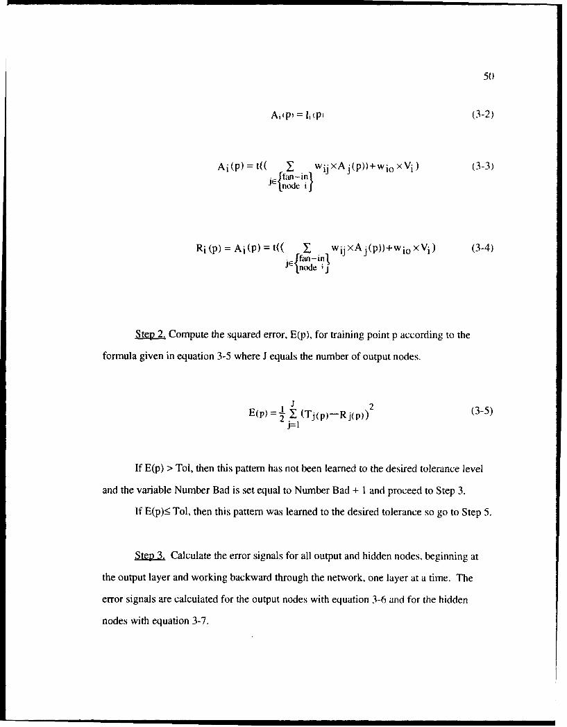
50
Ai(p, = li(Pj (3-2)
Ai(p) = t(( I wijxAj(p))+wioxVi) (3-3)Sfftan-inlJI ]node if
Ri (p) = Ai(P)=t(( Y-' wij×Aj(p))+Wio ×Vi) (3-4)• E frm- in],
Jnode ;{ j
Step 2, Compute the squared error, E(p), for training point p according to the
formula given in equation 3-5 where J equals the number of output nodes.
E Xp) = J I (Tj(p)-Rj(p)) (35)2j= 1
If E(p) > Tol, then this pattern has not been learned to the desired tolerance level
and the variable Number Bad is set equal to Number Bad + I and proceed to Step 3.
If E(p)< Tol, then this pattern was learned to the desired tolerance so go to Step 5.
S Calculate the error signals for all output and hidden nodes, beginning at
the output layer and working backward through the network, one layer at a time. The
error signals are calculated for the output nodes with equation 3-6 and for the hidden
nodes with equation 3-7.
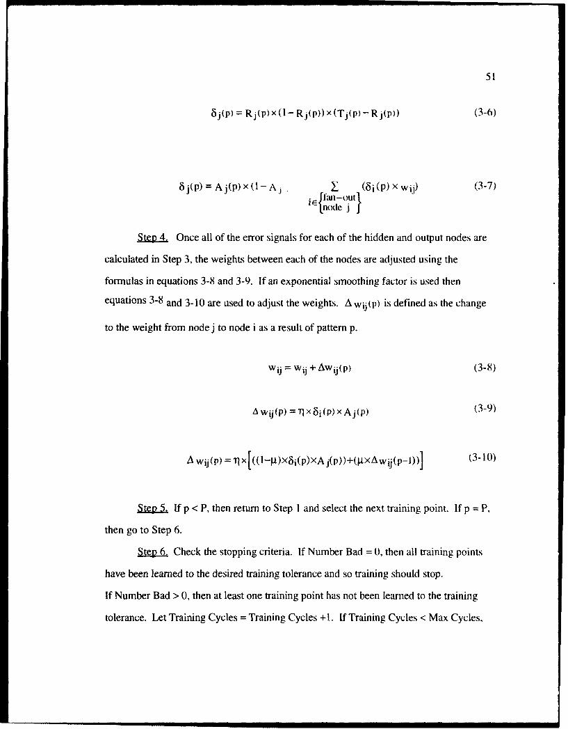
51
8j(P) = Rj(p)x (1- Rj(p)) x(Tj(p)-Rj(p)) (3-6)
8j(p) =A j(p)x( (6i(p) x wij) (3-7)i ffan-out 1
Inode j J
Ste 4. Once all of the error signals for each of the hidden and output nodes are
calculated in Step 3, the weights between each of the nodes are adjusted using the
formulas in equations 3-8 and 3-9. If an exponential smoothing factor is used then
equations 3-8 and 3-10 are used to adjust the weights. A wij(P) is defined as the change
to the weight from node j to node i as a result of pattern p.
wij = wij + Awij(p) (3-8)
A wij (p) = 7 x 6i (P) x Aj(p) (3-9)
A wij(P) = Ti X [(0(-II)Xii(p)XA j(p))+(QtxAwij (p-1))] (3-10)
Step 5. If p < P, then return to Step I and select the next training point. If p = P,
then go to Step 6.
S Check the stopping criteria. If Number Bad = 0, then all training points
have been learned to the desired training tolerance and so training should stop.
If Number Bad > 0, then at least one training point has not been learned to the training
tolerance. Let Training Cycles = Training Cycles +1. If Training Cycles < Max Cycles,

52
then go to Step I and begin another training cycle with the first training point, otherwise
stop.
The adjustment to the weights in Step 4 occurs as each training point is presented
to the network in what is known as pattern training. To implement true gradient descent
on the squared error surface would require the summation of the amount to change the
weights for each of the training points with the actual change only being made at the end
of each training cycle or epoch, in what is known as batch training. While BrainMaker has
an option to perform training in this manner, it was not used in this research since it is
more likely to become trapped in a local minimum of the error surface and it typically
results in an increase in training time.(1 33)
3.4 Summary
This chapter provides an overview of the research issues and the methodology
used to conduct the research in this dissertation. The research issues were developed and
refined throughout the researLt; effort. The methodology for conducting the research was
to use an inventory computer simulation to perform a series of experiments in building
ANN metamodels in order to develop a baseline ANN metamodel approach and to then
demonstrate the use of the approach on a more complicated computer simulation, namely
of an emergency department. Detailed discussion is included on the assumpti")ns and
restrictions of the research which are initially stated in Chapter 1. Specific details are
provided on the two commercial software packages used to perform the iesearch,
SIMAN/CINEMA and BrainMaker. The SIMAN/CINEMA package was used to perform
the stochastic computer simulations for the research problems. The BrainMaker package
implements backpropagation training on feedforward artificial neural networks.

53
4.0 DEVELOPMENT PROBLEM - INITIAL EXPERIMENTS INAPPROXIMATING AN (sS) INVENTORY SYSTEM
The approach taken in this research was to use a simple, yet realistic, model of a fairly
complex engineering system as a testbed for various methods to approximate computer
simuilations using artificial neural networks. This chapter covers the initial experiments
performed in approximating the computer simulation of an (s,S) inventory system with
ANN. Using this particular system permitted the focus to be on developing the
methodology of ANN approximation of computer simulations and not on computer
simulation issues.
4.1 Description of the (s,S) Inventory System
The system used as a development problem in this dissertation was taken from
Chapter 12 "Experimental Design and Optimization" by Law and Kelton.( 134) The system
is a probabilistic lot size-reorder point system, an (s,S) inventory system where s = reorder
point quantity, and S = order up to quantity, with a time horizon of 120 months. It is
difficult to obtain optimal solutions for these types of systems.(135) While progress has
been made in developing algorithms for determining optimal policies of certain infinite
time horizon versions of the (s, S) inventory problems, computer simulation is still
necessary for examining many of the possible variants of the (s, S) inventory problem.0 36)
Law and Kelton constructed a series of first- and second- order regression model
approximations, or metamodels, of a computer simulation of the inventory system. By
increasing the number of data points, they were able to demonstrate that the metamodels
could provide increasingly accurate approximations of the computer simulation.

54
The inventory system is representative of companies that sell a single product, with
the problem of deciding how many items to obtain from their supplier in each of the next n
months in order to minimize the total cost of the inventory system. There are several
input and output parameters associated with this system. The input parameters of the
simulation of the system include the following:
s = reorder point,
S = order up to quantity,
I = inventory level,
Z = reorder quantity,
d = S-s = reorder quantity when I = s,
D = size of demands,
td = time between demands,
to = time between order decisions,
tL = time lag for delivery,
k = setup cost,
i = incremental cost per item ordered,
h = holding cost,
u = underage cost (cost of having to backlog orders),
n = time horizon for analysis purposes.
In Law and Kelton's sample problem, the parameters s and d were the only
parameters that were treated as decision variables. The remaining input parameters were
treated as uncontrollable factors and were assumed to be fixed at constant values. The
following section describes the settings used for these uncontrollable factors, in Law and
Kelton and in this dissertation.

55
The initial inventory level was set at Io = 60. In this system it is assumed that the
company receives demands for its products on a periodic basis with the time between
demands, td, distributed exponential with a mean of 0.1 month. The size of each demand,
D is distributed according to equation 4-1.
JI with probability Y6
with probability X (4-1)
3 with probability Y,
4 with probability Y6
The time between order decisions, to, is one month. A stationary (s,S) policy is
used to decide how much to order at the beginning of each month. In other words, given
that I is the inventory at the beginning of the month, then the amount to order for that
month, Z, is determined by equation 4-2.
S-I ifl<sZj= ifI!s (4-2)
In this system, the company determines each month whether or not it should place
an order, and if so, how much to order. If an order is placed, then the time it takes for the
order to arrive at the company, tL, is distributed uniformly between 0.5 and I month. The
total order cost is equal to k + iZ. In this problem k = $32 and i = $3. The holding cost
per item per month held in inventory is given as h = $1. The underage cost is given as u =
$5 per item per month in backlog (i.e., on order). The underage costs include such items
as extra bookkeeping costs and loss of goodwill costs. The planning horizon or time that
the system would operate under the various strategies of operating the inventory system
was set at n = 120 months.

56
Some of the relevant output measures that could be calculated for this system,
over the planning horizon, include:
Average total cost (C),
Average ordering cost,
Average holding cost,
Average shortage cost,
Average inventory level,
Minimum inventory level,
Maximum inventory level.
Law and Kelton used the computer simulation of the inventory system to obtain
estimates of the output measure, average total cost per month (C) for various settings of
the decision variables s and d. Since Law and Kelton used the inventory system to discuss
the process of experimental design, they labeled the average total cost as R (for response
of the computer simulation).
4.2 Computer Simulation of the Inventory System
The inventory system computer simulation used in this dissertation was written in
the SIMAN simulation language for the reasons discussed in Chapter 3. Output statistics
of different input parameter settings from a computer simulation can be categorized as
either independent or dependent observations. In simulation, independent observations
have been used quite widely due to the applicability of straightforward statistical tests for
comparing alternatives. Dependent observations have been used for the purpose of
v u1wice reduction. One frequently used technique for producing dependent observations

57
is the common random number approach, one component of which is to use the same
starting point in the same random number streams for each input parameter setting in a
simulation run. Using the common random number approach would probably provide a
more stable, but less robust, set of observations from the computer simulation since the
variance is typically reduced. However, this research examined only the independent
observations approach. One way that independent observations are obtained is to select
different starting points in the same random number streams for each input parameter
setting. In this research, independent observations for each input parameter setting were
obtained by selecting the random number streams and running the simulation program
through all of the desired replications by having the computer simulation iteratively read
the input parameter settings from an external file. In this way the random number stream
was never reset to the original starting point and thus created independent observations for
all the replications of all of the input parameter settings. In some cases, due to memory
restrictions of the computer, additional replications were made using different random
number streams in order to preserve independence between the replications made for each
input parameter setting. The same procedure was followed for all of the experiments
performed in this research. For illustrative purposes the SIMAN computer programs and
external data files that were used to produce the independent observations for this section
are provided in Appendix A in Figures A l through A3.
Validation of the SIMAN computer simulation was performed by comparing the
output from the SIMAN simulation to the results given by Law and Kelton. Since Law
and Kelton only provided the output of single simulation replications, a direct statistical
comparison of the two is not possible. However, Law and Kelton did report the results of
building first-and second-order regression models on multiple replications for different

58
input parameter settings. The approach used to validate the SIMAN simulation model of
the inventory system was to build the same first- and second-order regression models on
the SIMAN simulation data and compare the regression results to those found in Law and
Kelton.
The two sets of input parameters given in Table 1 were simulated and used to build
regression models. Each parameter setting consisted of a different combination of values
of the input parameters s and d. The output measure of system performance, that was
provided by the simulation, was the 120 month average, of monthly total cost, C. The
SIMAN simulation results, where C is the average of C over ten replications, as well as
the two input parameter settings for data sets A and B, are provided in Table 1.
Table 2 shows the regression models that were used by Law and Kelton to develop
metamodels of the computer simulation. The Law and Kelton and SIMAN simulation
results of ten replications of data set A, the first four input parameter settings from Table
1, were approximated using the first-order multiple linear regression model given in Table
2. The second-order multiple linear regression model in Table 2 was used to model the
simulation results of five replications (from Law and Kelton) and ten replications (from
SIMAN) of data set B, the second set of 36 input parameter settings from Table 1. It is
not clear why Law and Kelton used only five replications at the 36 input parameters when
all of the rest of their examples used ten replications. To maintain consistency between
the models of the two data sets, ten replications were used in this dissertation for each
model. The regression model results for the SIMAN data for data sets A and B are
provided in Tables 3 and 4, respectively.
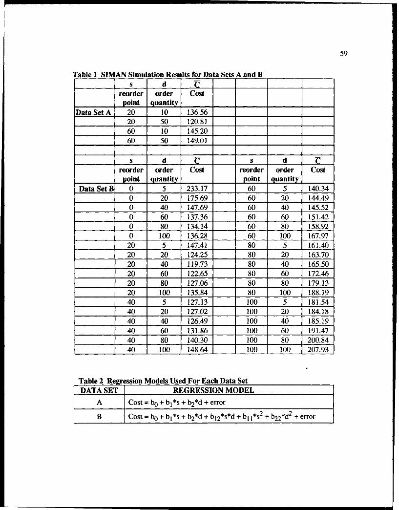
59
Table I SIMAN Simulation Results for Data Sets A and Bs d __
reorder order Costpoint quantity,
Data Set A 20 10 136.5620 50 120.81
60 10 145.2060 50 149.01
s d s d ireorder order Cost reorder order Costpoint quantity point quantity
Data Set B 0 5 233.17 60 5 140.340 20 175.69 60 20 144.490 40 147.69 60 40 145.52
0 60 137.36 60 60 151.420 80 134.14 60 80 158.92
0 100 136.28 60 100 167.9720 5 147.41 80 5 161.4020 20 124.25 80 20 163.7020 40 119.73 80 40 165.5020 60 122.65 80 60 172.4620 80 127.06 80 80 179.1320 100 135.84 80 100 188.1940 5 127.13 100 5 181.5440 20 127.02 100 20 184.1840 40 126.49 100 40 185.1940 60 131.86 100 60 191.4740 80 140.30 100 80 200.8440 100 148.64 100 100 207.93
Table 2 Regression Models Used For Each Data SetDATA SET REGRESSION MODEL
A Cost = b0 + bl*s + b2 *d + error
B Cost = b0 + bl*s + b2 *d + bl 2 *s*d + bI*s2 + b22*d2 + error
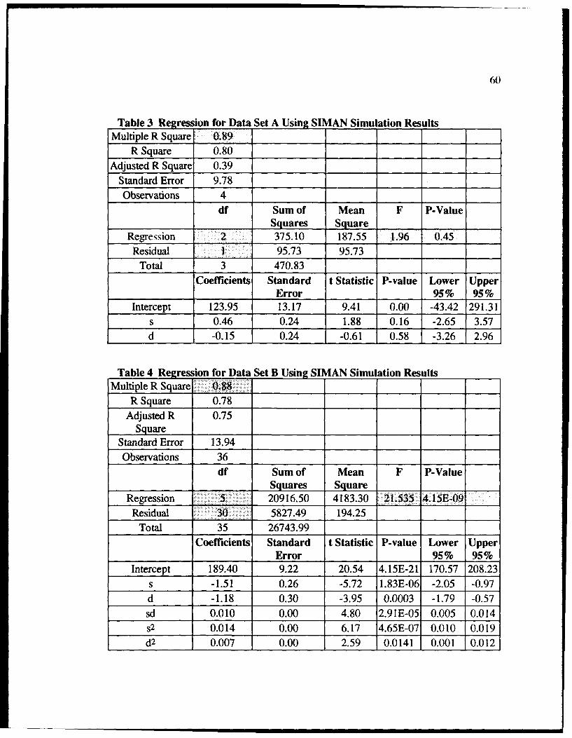
60
Table 3 Regression for Data Set A Using SIMAN Simulation ResultsMultiple R Square. 0.89 _______ __
R Square 0.80
Adjusted R Square 0.39
Standard Error 9.78
Observations 4df Sum of Mean F P-Value
Squares Square
Regression 2 375.10 187.55 1.96 0.45 ....
Residual 1 95.73 95.73Total 3 470.83
Coefficients Standard t Statistic P-value Lower UpperError 95% 95%
Intercept 123.95 13.17 9.41 0.00 -43.42 291.31s 0.46 0.24 1.88 0.16 -2.65 3.57d -0.15 0.24 -0.61 0.58 -3.26 2.96
Table 4 Regression for Data Set B Using SIMAN Simulation ResultsMultiple R Square 088
R Square 0.78
Adjusted R 0.75Square
Standard Error 13.94
Observations 36df Sum of Mean F P-Value
Squares SquareRegression 5 20916.50 4183.30 21-535 4.15E-09
Residual 30 5827.49 194.25
Total 35 26743.99
Coefficients Standard t Statistic P-value Lower UpperError 95% 95%
Intercept 189.40 9.22 20.54 4.15E-21 170.57 208.23s -1.51 0.26 -5.72 1.83E-06 -2.05 -0.97d -1.18 0.30 -3.95 0.0003 -1.79 -0.57sd 0.010 0.00 4.80 2.91E-05 0.005 0.014S2 0.014 0.00 6.17 4.65E-07 0.010 0.019
d2 0.007 0.00 2.59 0.0141 0.001 0.012

61
As can be seen from Tables 3 and 4 both models have approximately the same
multiple R square values. The regression models in Tables 3 and 4 were built using the
averages of the 10 replications at each data point. The same results in terms of the model
coefficients result if the individual replications are used instead of the averages. However,
in the regression model built on individual replications, the apparent goodness of the
model increases due to a more significant F statistic caused by an increase in the degrees
of freedom. In summary, the models provided by regression are the same for both
averages and individual replications.
TABLE 5 Estimates of Regression Model Coefficients
DATA SIMULATION REGRESSION MODEL
SET DATA
"A SIMAN Cost= 123.95+0.46s-0.15d
"A LAW & KELTON Cost = 125.37+0.44s-0.22d
B SIMAN Cost= 189.40-1.51s-1.18d+.OlOsd+.014s2+.007d 2
B LAW & KELTON Cost= 188.51-1.49s-1.24d+.OlOsd+.014s 2+.007d2
A summary of the regression results for each model in Table 2 is provided in Table
5 for both SIMAN and Law and Kelton simulation data.U37) There is close agreement in
the coefficients of the regression equations for the SIMAN simulation data and the Law
and Kelton simulation data for both data sets A and B. As can be seen from Tables 3 and
4, the 95% confidence intervals for each of the regression coefficients of the SIMAN data
contain the regression coefficients obtained by Law and Kelton. Thus, for a Type I error
of o = 0.05, we do not have enough evidence to reject the null hypothesis that the SIMAN
and Law and Kelton regression models are the same. This indicates that the SIMAN
computer simulation models used in this research provide results that are similar to those
produced by the computer simulations developed by Law and Kelton.

62
It should be noted that the last three values in the equation for Law and Kelton for
data set B in Table 5 are mislabeled in the Law and Kelton textbook.134) This can be seen
by solving for the minimum of the function. The minimum value for the function in the
textbook is found at s = 148 and d = - 42. By making the changes found in the table, in
row D*, the minimum value is found at s = 29 and d= 68. These changes are also
consistent with the contour diagrams of the function found in textbook and in Figure 9a
discussed below.
Figure 9 shows three surface and contour plots of the space formed by s, d and
cost as determined by direct simulation, a regression metamodel and an ANN metamodel.
Figure 9a shows the surface plot and a contour plot of 420 equally spaced points on the
(s,d) grid with the height of the surface and the contour lines representing the cost for
each combination of s and d as determined by ten replications of direct simulation. This is
basically the target that the metamodels are attempting to approximate. The regression
model approximation to the target from Table 5, which was built on the 36 data points of
set B, is shown in Figure 9b. As can be seen in Figure 9b, the model is smoother and has
values that are too low in the lower left hand corner and values that are too high in the
upper right hand comer. An artificial neural network approximation built on the same 36
data points of set B, is shown in Figure 9c. Visually, it appears that the ANN metamodel
captures the essence of the surface better than the regression metamodel. In addition, the
mean absolute error of the ANN evaluated at all 420 test points is 3.20 while the MAE is
8.64 for the regression model.( 138)
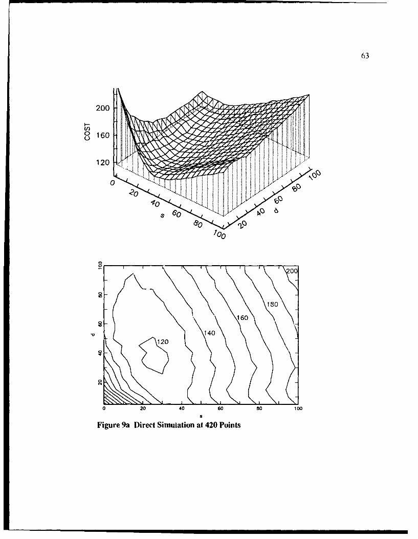
63
16
120
06
7000
00
180
1600-
V 140120
(.4
0 20 40 60 so 100
Figure 9a Direct Simuiation at420 Points
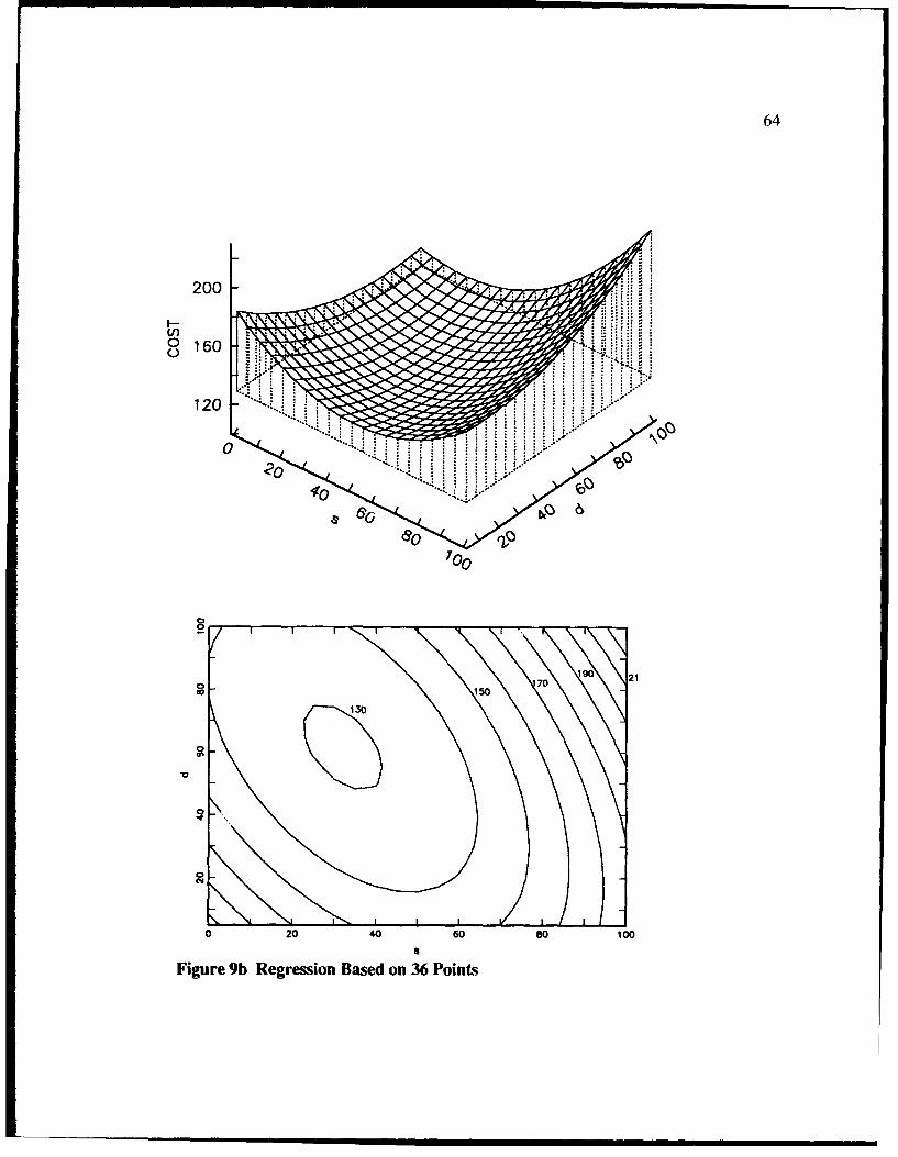
64
200
10
0
430
06
70
13
0 20 40 60 80 100
Figure 9b Regression Based on 36 Point;
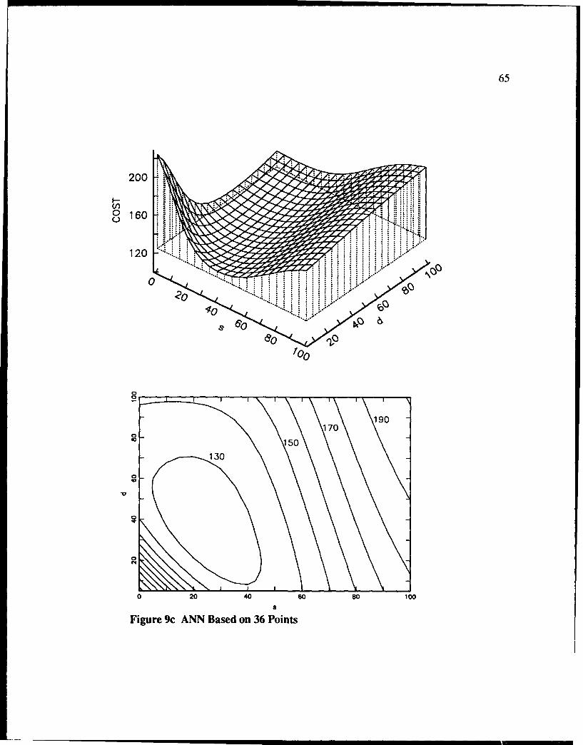
65
2004
F-
o 160 F.
012 0 = :=LY
......
IPO
630
0 20 40 60 0 100
a
Figure 9c ANN Based on 36 Points
l | | •7|

66
4.3 Experiments with Two Simulation Input Parameters
This set of experiments consisted of two different experiments. The first
experiment consisted of predicting a single simulation output, mean cost. The second
experiment predicted four typical descriptive statistics produced by computer simulations
(i.e., mean, standard deviation, minimum, maximum).
The simulation of each input parameter setting consisted of operating the inventory
system for a period of 120 months, or ten years of simulated time. The statistics used in
these two experiments are calculated on the basis of the 120 months of operating the
inventory system within each replication. Thus, at the end of each replication over the 120
months there is a minimum cost month, a maximum cost month and it is possible to
calculate the average monthly cost and the standard deviation of the monthly costs.
Finally, for each input parameter setting, multiple replications are performed and each of
the relevant statistics are captured for each replication.
The purpose of these experiments is to examine the manner and the amount of
simulation data to use in training an ANN to predict typical computer simulation outcome
measures. One obvious way was to use just the average output values of the computer
simulation replications at each input parameter setting. This seemed to eliminate
information that the ANN might be able to take advantage of in building a better model of
the computer simulation. Thus, the opposite extreme of using all of the simulation
replications was also considered. Preliminary experiments showed that unlike regression,
ANN metamodels built using averaged replication data performed differently than ANN
built on individual replications. Concern about the effect of extreme points in the
simulation data led to consideration of additional methods which used only the fifty

67
percent of the data that was nearest to the mean value. Finally, combinations of using
averages and replications were also considered.
Specifically, five different methods of presenting simulation data to ANN were
examined. The methods ranged from presenting all the individual replications to just the
averages of the replications. The five presentation methods were:
Presentation Method 1 - Average output of all simulation replications.
Presentation Method 2 - All simulation replications and the average of all
simulation replications.
Presentation Method 3 - Half of the simulation replications nearest to the average
and the average of all simulation replications.
Presentation Method 4 - All simulation replications.
Presentation Method 5 - Half of the simulation replications nearest the average.
For each presentation method, the effect of increasing the number of simulation
replications was examined. The number of replications of the computer simulation used
for each input parameter setting was n = 1, 2, 3, 4, 5, 6, 7, 8, 9, 10, 15, 20, and 25.
The input parameter settings that were used to obtain data from the computer
simulation to train the ANN for these experiments are shown in Table 6. As can be seen
from Table 6, only two input parameters were allowed to vary: s and d. For illustrative
purposes, the results of the computer simulation for each of the combinations of the input
parameters shown in Table 6 for Experiment 1 and Experiment 2 for the average of 25
replications are provided in Appendix A, Table A l and Table A2, respectively.

68
Table 6 Training Input Parameter Settings for Experiments I and 2Input Parameter Combinations of Trainin Input Parameter Settings
s 20 40 60 80 20 40 60 80d 20 20 20 20 40 40 40 40
s 20 40 60 80 20 40 60 80d 60 60 60 60 80 80 80 80
The data used to test the ANN was obtained by running the computer simulation at
the input parameter settings shown in Table 7. The test data was used to examine the
ability of the ANN to generalize to previously unseen examples. The test set consisted of
points that were completely internal to the training set and points that were completely
external to the training set. The third grouping that was evaluated was the combination of
all of the internal and external points. It was assumed that the average of the outputs of
500 replications for each input parameter setting of the test set from the computer
simulation were the "right" answers. The metric for comparison purposes was the mean
absolute error (MAE) of the difference between the outputs of the ANN and the computer
simulations "right" answers. The test set "right" answers are provided in Appendix A,
Tables A3 and A4, for experiments I and 2 respectively. A graphical portrayal of the
location of the various training and test sets is given in Figure 10.
Table 7 Testing Input Parameter Settings for Experiments I and 2Data Set Input Combinations of Testing Input Parameter
Parameter SettingsInternal s 30 50 70 30 50 70 30 50 709points d 30 30 30 50 50 50 70 70 70
External s 10 50 90 10 90 10 50 908po ints d 10 10 10 50 50 90 90 901
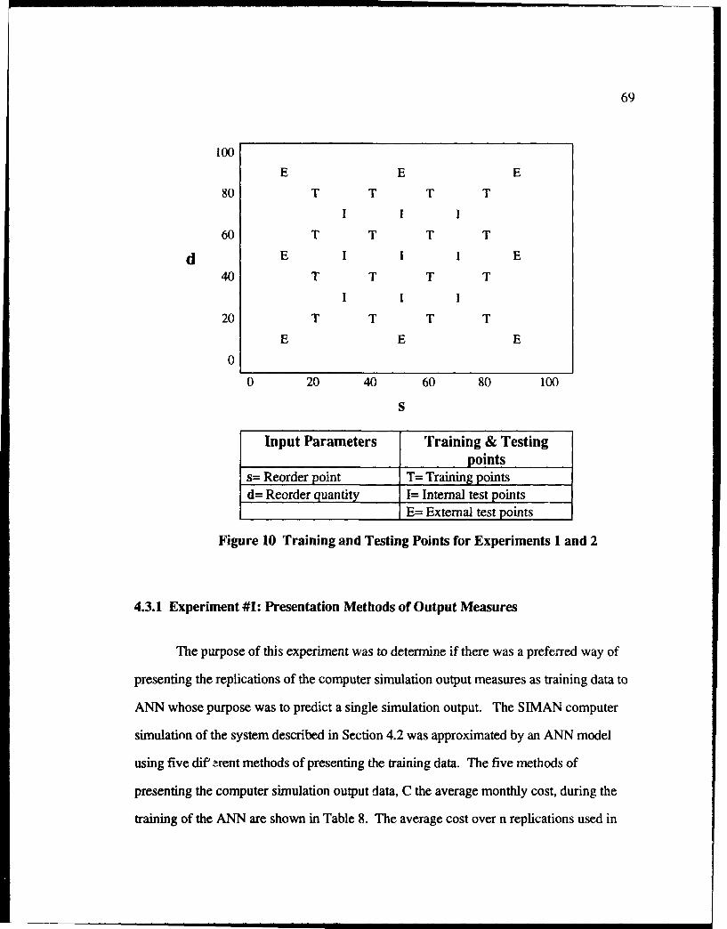
69
100
E E E80 T T T T
I I I
60 T T T T
d E I E
40 T T T TI
20 T T T T
E E E
0
0 20 40 60 80 100
S
Input Parameters Training & Testing
pointss= Reorder point T= Training pointsd= Reorder quantity 1= Internal test points
IE= External test points
Figure 10 Training and Testing Points for Experiments I and 2
4.3.1 Experiment #1: Presentation Methods of Output Measures
The purpose of this experiment was to determine if there was a preferred way of
presenting the replications of the computer simulation output measures as training data to
ANN whose purpose was to predict a single simulation output. The SIMAN computer
simulation of the system described in Section 4.2 was approximated by an ANN model
using five dif -rent methods of presenting the training data. The five methods of
presenting the computer simulation output data, C the average monthly cost, during the
training of the ANN are shown in Table 8. The average cost over n replications used in
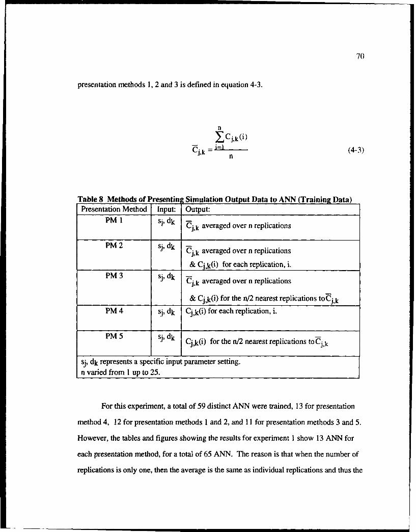
70
presentation methods 1, 2 and 3 is defined in equation 4-3.
n
ICj,k(i)
Cj,k = i=l n(4-3)jk n
Table 8 Methods of Presenting Simulation Output Data to ANN (Training Data)Presentation Method Input: Output:
PM 1 si, dkCj,k averaged over n replications
PM2 sj, dkCj,k averaged over n replications
_______________ ______ & Cj,k(i) for each replication, i.PM 3 sj, dk --
Cj,k averaged over n replications
& Cjk(i) for the n/2 nearest replications toCj,k
PM 4 sj, dk Cjk(i) for each replication, i.
PM 5 sjdk Cj,k(i) for the n/2 nearest replications to Cj,k
sj, dk represents a specific input parameter setting.n varied from 1 up to 25.
For this experiment, a total of 59 distinct ANN were trained, 13 for presentation
method 4, 12 for presentation methods 1 and 2, and 11 for presentation methods 3 and 5.
However, the tables and figures showing the results for experiment I show 13 ANN for
each presentation method, for a total of 65 ANN. The reason is that when the number of
replications is only one, then the average is the same as individual replications and thus the
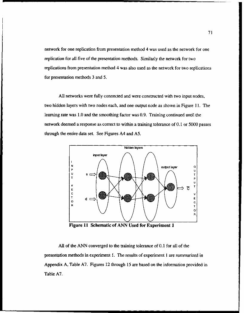
71
network for one replication from presentation method 4 was used as the network for one
replication for all five of the presentation methods. Similarly the network for two
replications from presentation method 4 was also used as the network for two replications
for presentation methods 3 and 5.
All networks were fully connected and were constructed with two input nodes,
two hidden layers with two nodes each, and one output node as shown in Figure 11. The
learning rate was 1.0 and the smoothing factor was 0.9. Training continued until the
network deemed a response as correct to within a training tolerance of 0.1 or 5000 passes
through the entire data set. See Figures A4 and A5.
hidden layers
input layer
N Output layer 0P U
U TT P
UV TEC VT dc E
0 CR T
0
Figure 11 Schematic of ANN Used for Experiment 1
All of the ANN converged to the training tolerance of 0. 1 for all of the
presentation methods in experiment 1. The results of experiment I are summarized in
Appendix A, Table A7. Figures 12 through 15 are based on the information provided in
Table A7.
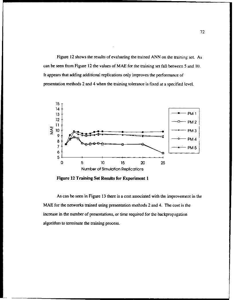
72
Figure 12 shows the results of evaluating the trained ANN on the training set. As
can be seen from Figure 12 the values of MAE for the training set fall between 5 and 10.
It appears that adding additional replications only improves the performance of
presentation methods 2 and 4 when the training tolerance is fixed at a specified level.
151413 - PM 112 0 PM 2
< 10
0 PM 3I -9" A --- 0-- PM 4
7 ,L PM 565 I I I I I
0 5 10 15 20 25Number of Simulation Replications
Figure 12 Training Set Results for Experiment 1
As can be seen in Figure 13 there is a cost associated with the improvement in the
MAE for the networks trained using presentation methods 2 and 4. The cost is the
increase in the number of presentations, or time required for the backpropagation
algorithm to terminate the training process.
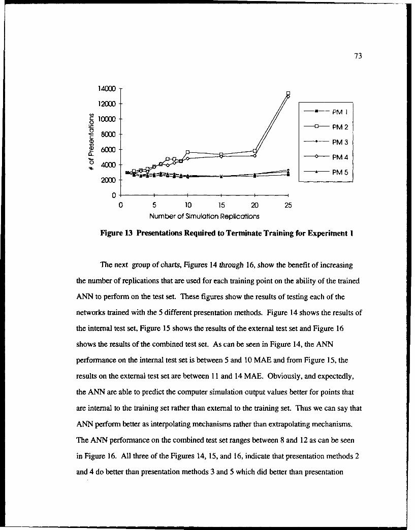
73
14000-
12000PM 1
C 10000-.2 -0 PM 24- 8000 Oa) -- PM 3
6.000 - PM 4
o 4000-_ __ A PM 5
2000
0 I I I II
0 5 10 15 20 25
Number of Simulation Replications
Figure 13 Presentations Required to Terminate Training for Experiment 1
The next group of charts, Figures 14 through 16, show the benefit of increasing
the number of replications that are used for each training point on the ability of the trained
ANN to perform on the test set. These figures show the results of testing each of the
networks trained with the 5 different presentation methods. Figure 14 shows the results of
the internal test set, Figure 15 shows the results of the external test set and Figure 16
shows the results of the combined test set. As can be seen in Figure 14, the ANN
performance on the internal test set is between 5 and 10 MAE and from Figure 15, the
results on the external test set are between 11 and 14 MAE. Obviously, and expectedly,
the ANN are able to predict the computer simulation output values better for points that
are internal to the training set rather than external to the training set. Thus we can say that
ANN perform better as interpolating mechanisms rather than extrapolating mechanisms.
The ANN performance on the combined test set ranges between 8 and 12 as can be seen
in Figure 16. All three of the Figures 14, 15, and 16, indicate that presentation methods 2
and 4 do better than presentation methods 3 and 5 which did better than presentation
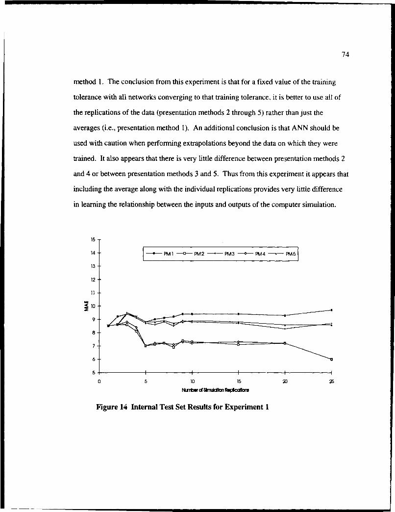
74
method 1. The conclusion from this experiment is that for a fixed value of the training
tolerance with all networks converging to that training tolerance. it is better to use all of
the replications of the data (presentation methods 2 through 5) rather than just the
averages (i.e., presentation method 1). An additional conclusion is that ANN should be
used with caution when performing extrapolations beyond the data on which they were
trained. It also appears that there is very little difference between presentation methods 2
and 4 or between presentation methods 3 and 5. Thus from this experiment it appears that
including the average along with the individual replications provides very little difference
in learning the relationship between the inputs and outputs of the computer simulation.
15
14 PtPMi1 a PM2 PM3 *PM4 - PM5
13
12
10
9-
8
7 -
6
5.I I I I
0 5 10 15 2) 25
Figure 14 Internal Test Set Results for Experiment I
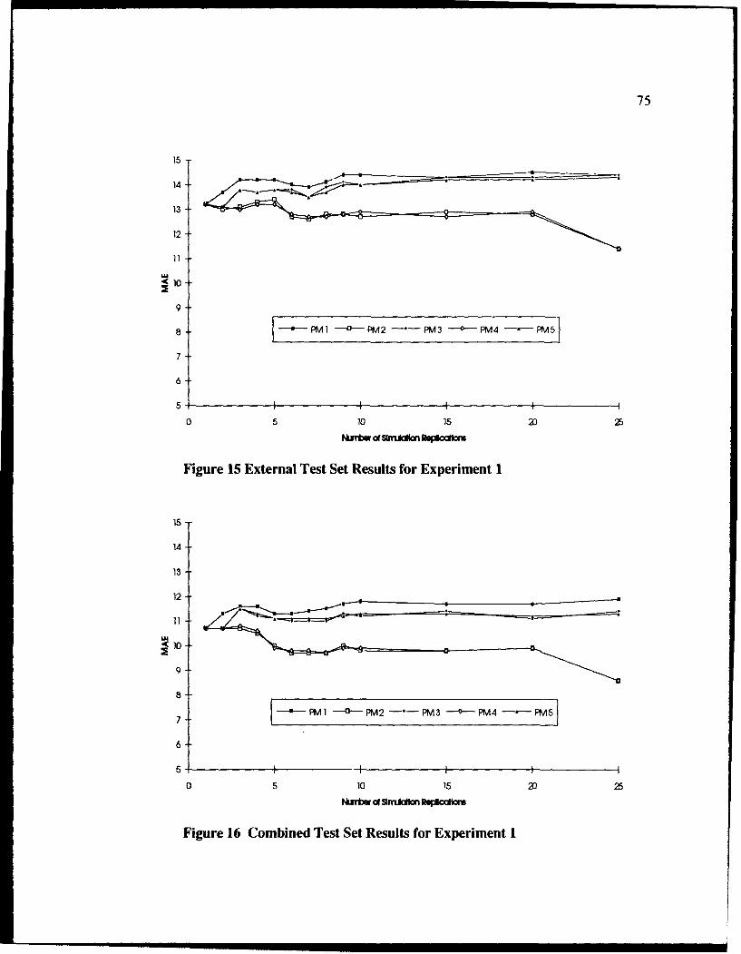
75
14-
13
12
11
LU<10
9
8- 'PMI cPM2 FM3 ~PM4 ~PMv5
7
6
5
0 5 10 15 20 25
Mxntmn df Simicion Ovopiccfm
Figure 15 External Test Set Results for Experiment 1
15-
14-
13 -
11 _______
<10
9-
8-
6-
0 5 10 15 23 25
Figure 16 Combined Test Set Results for Experiment 1

76
4.3.2 Experiment #2: Predicting Descriptive Statistics Typically Produced byComputer Simulations (Mean, Standard Deviation, Min and Max)
The major difference between experiment 1 and experiment 2 is that experiment 2
used the ANN to predict three additional aspects of the desired measure of effectiveness.
Both experiment I and 2 predict the mean value of the cost of operating the inventory
system for 120 months. Experiment 2 also predicted the standard deviation, minimum and
the maxllwm value of the cost for the same time period. These measures of cost are
typical outputs provided by most computer simulation packages as the output of a single
replication of the simulation. An example of the training data used for experiment 2 is the
averages (i.e., presentation method 1) of the four different aspects of cost for 25
replications which is given in Table A2 of appendix A. The distinction between the
internal, external and combined test points was examined in experiment I but was not
considered in experiment 2. The only test set examined in experiment 2 was the combined
test set which is provided in Table A4 in Appendix A.
For this experiment, a total of 59 different ANN were developed. All networks
were fully connected and were constructed with two input nodes, two hidden layers with
ten nodes each, and four output nodes. These networks have five times as many hidden
nodes as were used in experiment 1, because it is a much harder problem to learn four
outputs than to learn one output. Initial trials with a varying number of hidden nodes in
each hidden layer yielded 10 hidden nodes per layer as a good starting point for this
particular problem. Each input node corresponded to one of the input parameters (s, d),
and each output node corresponded to one of the output parameters (mean, standard
deviation, minimum, maximum). The learning rate was 1.0 and the smoothing factor was
0.9. Training continued until the network deemed a response as correct to within a

77
training tolerance of 0.1 for each of the four outputs or 5000 passes through the entire
data set (See Figures A6 and A7).
The only presentation method to have all of the networks converge to the training
tolerance of 0.1 for experiment 2 was the first presentation method. The results of
experiment 2 are summarized in Appendix A, Table A8 for the training sets and Table A9
for the test set. The charts in Figures 17 through 25 are based on the information
provided in Tables A8 and A9. The results in Tables A8 and A9 suggest, as was seen in
experiment 1, that there is very little difference between presentation methods 2 and 4 or
between presentation methods 3 and 5. Therefore, the figures showing the results for
experiment 2 do not include presentation methods 4 and 5.
The results of the network evaluations of the training set for the various number of
simulation replications for presentation methods one, two and three for the mean, standard
deviation, minimum value, and maximum value of cost are shown in Figures 17, 18, 19
and 20, respectively. From these graphs it appears that there is some interference taking
place between the various output measures that the neural networks are trying to learn. It
appears from the fairly random nature of the Mean Absolute Error (MAE) for mean cost
and minimum value of cost as seen in Figures 17 and 19 that this experiment has produced
ANN that are not very consistent even for very small changes in the number of replications
used to develop the ANN. This erratic behavior occurs for all of the presentation methods
including the converging presentation method 1. The MAE for the outputs of standard
deviation of cost and maximum value of cost as shown in Figures 18 and 20 are much
moie stable. An examination of the root mean square error (RMSE) for these measures in
Table A7 and A8 in Appendix A, show that RMSE is much larger than MAE for the
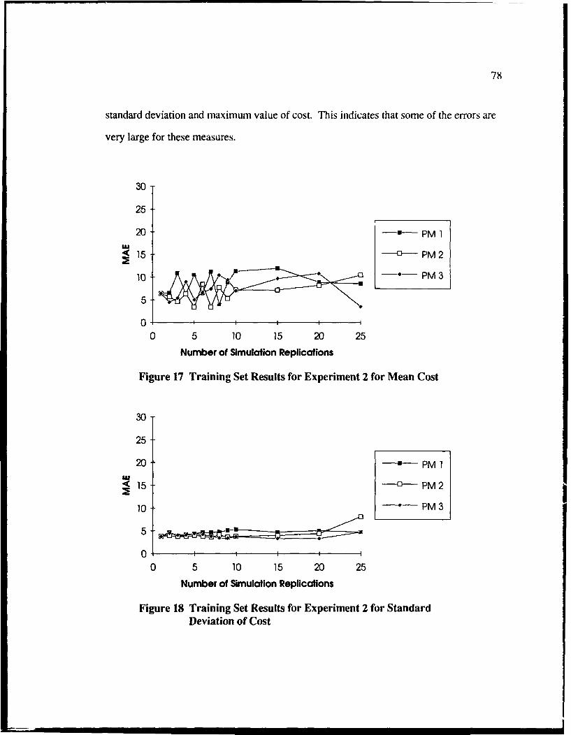
78
standard deviation and maximum value of cost. This indicates that some of the errors are
very large for these measures.
30
25
20 - PM 1
<15 -0---- PM 2
10- *- PM 3
5-
0 5 10 15 20 25
Number of Simulation Replications
Figure 17 Training Set Results for Experiment 2 for Mean Cost
30
25
20 = PM 1
S15 P- PM2
10-* PM 3
0 I t I
0 5 10 15 20 25
Number of Simulation Replications
Figure 18 Training Set Results for Experiment 2 for StandardDeviation of Cost
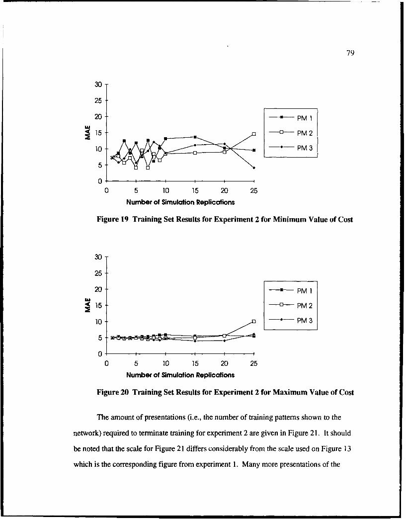
79
30
25
20- - PM 1
< 15, ----- PM 2
10- - PM 3
5
0 I I III
0 5 10 15 20 25
Number of Simulation Replications
Figure 19 Training Set Results for Experiment 2 for Minimum Value of Cost
30
25
20-" PM 1
<15 -- - PM 2
10 , PM 3
5
o I I t
0 5 10 15 20 25
Number of Simulation Replications
Figure 20 Training Set Results for Experiment 2 for Maximum Value of Cost
The amount of presentations (i.e., the number of training patterns shown to the
network) required to terminate training for experiment 2 are given in Figure 21. It should
be noted that the scale for Figure 21 differs considerably from the scale used on Figure 13
which is the corresponding figure from experiment 1. Many more presentations of the
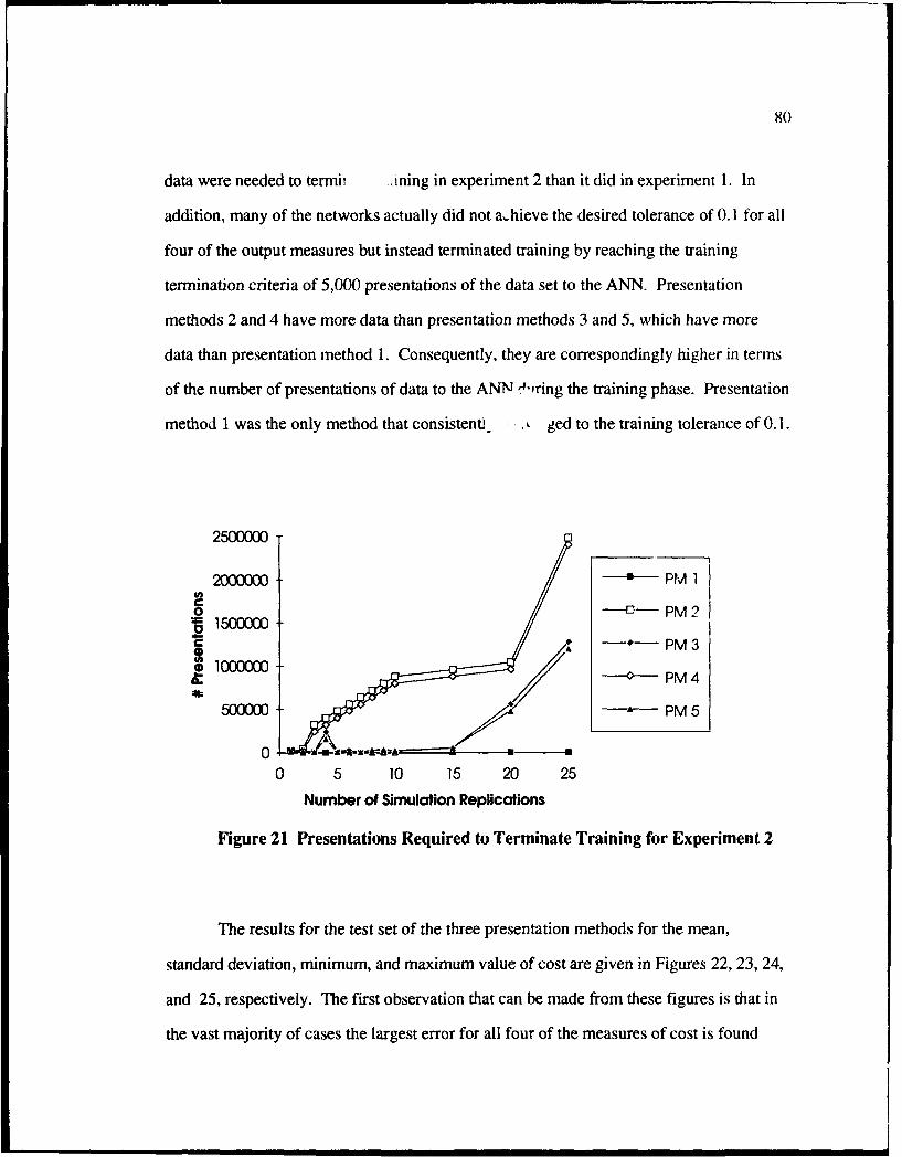
80
data were needed to termii Lrning in experiment 2 than it did in experiment 1. In
addition, many of the networks actually did not a,hieve the desired tolerance of 0.1 for all
four of the output measures but instead terminated training by reaching the training
termination criteria of 5,000 presentations of the data set to the ANN. Presentation
methods 2 and 4 have more data than presentation methods 3 and 5, which have more
data than presentation method 1. Consequently, they are correspondingly higher in terms
of the number of presentations of data to the ANN '4'ring the training phase. Presentation
method 1 was the only method that consistent). ged to the training tolerance of 0.1.
2500000
2000000 = PM 1C -a-- PM?0 PS1500000
-- PM3
-PM 4
500000 - PM 5
0-0 5 10 15 20 25
Number of Simulation Replications
Figure 21 Presentations Required to Terminate Training for Experiment 2
The results for the test set of the three presentation methods for the mean,
standard deviation, minimum, and maximum value of cost are given in Figures 22, 23, 24,
and 25, respectively. The first observation that can be made from these figures is that in
the vast majority of cases the largest error for all four of the measures of cost is found

81
with presentation method 1. There does not appear to be much of a difference in the
performance of presentation methods 2 and 3. The second observation is that the erratic
performance of the ANN in predicting mean and minimum cost that was present in the
training data is also present in the testing data. Comparing the appropriate charts (i.e.,
Figure 17 versus 22, Figure 18 versus 23, Figure 19 versus 24 and Figure 20 versus 25),
it is apparent that there is a larger degradation in the performance of networks on testing
data compared to training data for mean value and minimum value of cost than for the
standard deviation and maximum value of cost.
25 -
20-= PM 1
, 15 - - PM 2
10-- PM 3
5-2
I I
0 5 10 15 20 25
Number of Simulation Replications
Figure 22 Test Set Results for Experiment 2 for Mean Cost
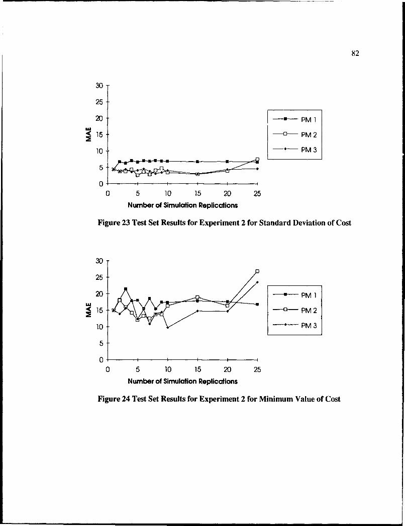
82
30
25
20 -- PM 1
"<15 ----- PM 2
10 -- PM 3
0 I I I II
0 5 10 15 20 25
Number of Simulation Replications
Figure 23 Test Set Results for Experiment 2 for Standard Deviation of Cost
30
25
-L-- PM 1
15___ 0 PM 2
10I PM 3
5-
0-0 5 10 15 20 25
Number of Simulation Replications
Figure 24 Test Set Results for Experiment 2 for Minimum Value of Cost
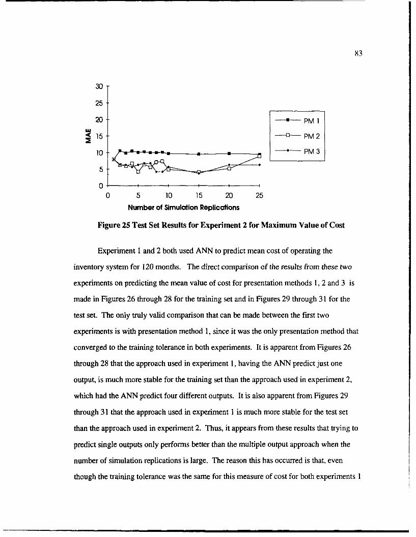
83
30
25
20 ----- PM 1
<15 0- PM 2
10_____ ____ -- PM 3552
0 5 10 15 20 25Number of Simulation Replications
Figure 25 Test Set Results for Experiment 2 for Maximum Value of Cost
Experiment I and 2 both used ANN to predict mean cost of operating the
inventory system for 120 months. The direct comparison of the results from these two
experiments on predicting the mean value of cost for presentation methods 1, 2 and 3 is
made in Figures 26 through 28 for the training set and in Figures 29 through 31 for the
test set. The only truly valid comparison that can be made between the first two
experiments is with presentation method 1, since it was the only presentation method that
converged to the training tolerance in both experiments. It is apparent from Figures 26
through 28 that the approach used in experiment 1, having the ANN predict just one
output, is much more stable for the training set than the approach used in experiment 2,
which had the ANN predict four different outputs. It is also apparent from Figures 29
through 31 that the approach used in experiment I is much more stable for the test set
than the approach used in experiment 2. Thus, it appears from these results that trying to
predict single outputs only performs better than the multiple output approach when the
number of simulation replications is large. The reason this has occurred is that, even
though the training tolerance was the same for this measure of cost for both experiments 1
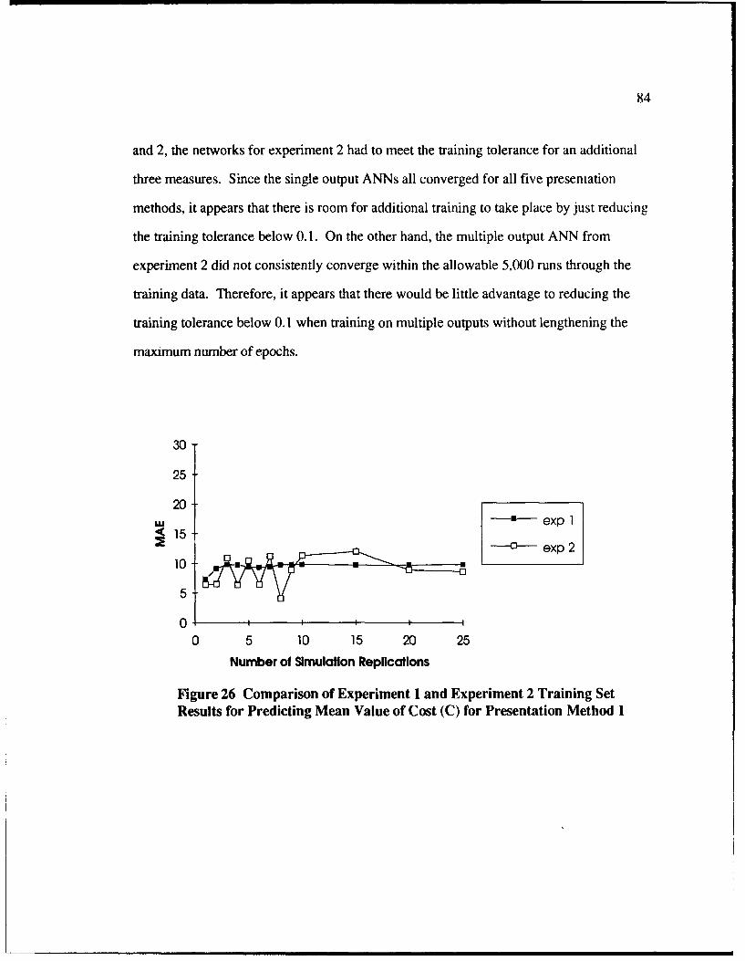
84
and 2, the networks for experiment 2 had to meet the training tolerance for an additional
three measures. Since the single output ANNs all converged for all five presentation
methods, it appears that there is room for additional training to take place by just reducing
the training tolerance below 0.1. On the other hand, the multiple output ANN from
experiment 2 did not consistently converge within the allowable 5,000 runs through the
training data. Therefore, it appears that there would be little advantage to reducing the
training tolerance below 0.1 when training on multiple outputs without lengthening the
maximum number of epochs.
30
25
20exp I
1< 150-- exp 2
10
5
0 I I I I
0 5 10 15 20 25
Number of Simulation Replications
Figure 26 Comparison of Experiment I and Experiment 2 Training SetResults for Predicting Mean Value of Cost (C) for Presentation Method 1
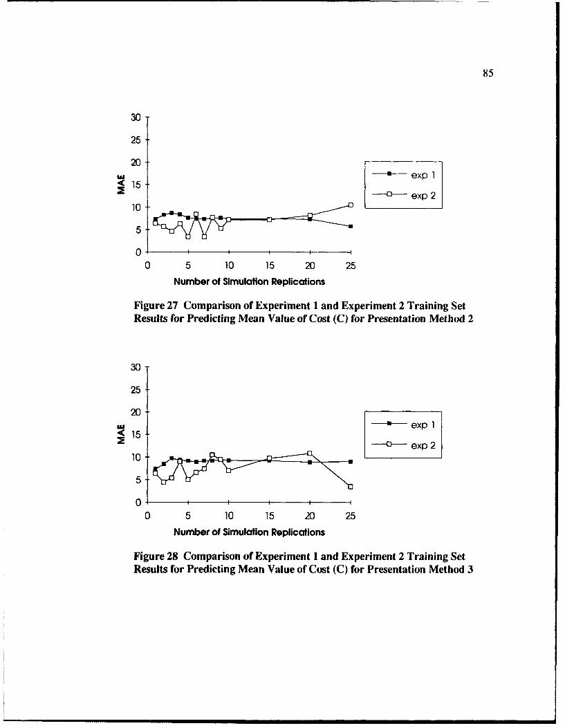
85
30
25
20w~ -- exp 1'<15 S-5 - exp 2
10
5-
0 I I I
0 5 10 15 20 25
Number of Simulation Replications
Figure 27 Comparison of Experiment I and Experiment 2 Training SetResults for Predicting Mean Value of Cost (C) for Presentation Method 2
30
25
20=U exp 1
<15 --• exp 2
10.
5-
0 I I t I I
0 5 10 15 20 25
Number of Simulation Replications
Figure 28 Comparison of Experiment I and Experiment 2 Training SetResults for Predicting Mean Value of Cost (C) for Presentation Method 3
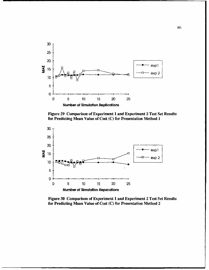
96
30
25
2020 expl
-a- exp 210 n
5
0 I I I I
0 5 10 15 20 25
Number of Simulation Replications
Figure 29 Comparison of Experiment I and Experiment 2 Test Set Resultsfor Predicting Mean Value of Cost (C) for Presentation Method 1
30
25
20=- exp1< 15--
1 0 exp 2
5
0 I II I I
0 5 10 15 20 25
Number of Simulation Reptications
Figure 30 Comparison of Experiment I and Experiment 2 Test Set Resultsfor Predicting Mean Value of Cost (C) for Presentation Method 2
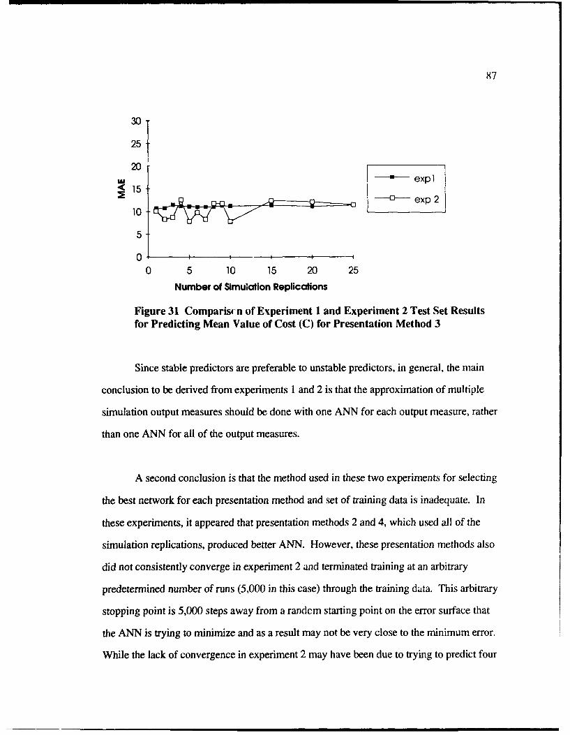
87
30
25
<• 1510 / • D- ,•.• ••'__ .g-•---• -- a•exp 2
0 I I I
0 5 10 15 20 25
Number of Simulation Replications
Figure 31 Comparisrn of Experiment I and Experiment 2 Test Set Resultsfor Predicting Mean Value of Cost (C) for Presentation Method 3
Since stable predictors are preferable to unstable predictors, in general, the main
conclusion to be derived from experiments 1 and 2 is that the approximation of multiple
simulation output measures should be done with one ANN for each output measure, rather
than one ANN for all of the output measures.
A second conclusion is that the method used in these two experiments for selecting
the best network for each presentation method and set of training data is inadequate. In
these experiments, it appeared that presentation methods 2 and 4, which used all of the
simulation replications, produced better ANN. However, these presentation methods also
did not consistently converge in experiment 2 and terminated training at an arbitrary
predetermined number of runs (5,000 in this case) through the training data. This arbitrary
stopping point is 5,000 steps away from a randcm starting point on the error surface that
the ANN is trying to minimize and as a result may not be very close to the minimum error.
While the lack of convergence in experiment 2 may have been due to trying to predict four

88
different output values, the following discussion shows that it could be due to another
problem. That is, by virtue of the stochastic nature of computer simulations, there are
different values produced by the computer simulation for the outl ut of a specific
combination of input parameter settings. For any given set of training data, there is at
least one input parameter setting that has the largest difference between its multiple
outputs, say MAXRANGE. If the desired training tolerance is smaller than
MAXRANGE/2 then the network will fail to converge if all of the simulation output
replications (i.e., presentation methods 2 or 4) are used as the training set. Thus, even
though in these first two experiments presentation methods that use all of the replicated
data did better than the presentation method that used the averages, it is quite possible that
for a particular training tolerance level the presentation methods could not converge. The
result would then be the final network, which in a sense is just a random point on the path
from the starting point to the minimum on the error surface. There is no guarantee that
such a point would be a very good point. In addition, if the training tolerance is small
enough, it is possible for presentation method I to not converge within a pre-specified
number of runs through the training data.
One way to avoid this problem is to pick a particular architecture for the ANN, use
the termination criterion of "maximum number of runs" and write the results of the
training performance to a file after each run through the training data. A search through
the training results file will determine which run through the data produced the network
with the best performance on the training set. Training without testing would then be
conducted for tho number of runs required to reach the best network. This procedure will
be referred to as "best net training" and is used throughout the remainder of the
dissertation. Another procedure that is similar is called "test and save" in which the

89
network is tested at pre-specified intervals and the networks are sived to individual files.
If the networks are saved after each training run through the data, then the networks
resulting from "best net training" and "test and save training" will be the same. Using the
"test and save" training procedure does not require a second training session to obtain the
weights of the best network. However, with the "test and save" procedure, it takes a lot
of time to write the individual networks to different files, it takes a lot of memory to hold
all of the files, and if the interval between testing networks is larger than one, then there is
no guarantee of finding the best network. For these reasons "test and save" was not used
in this research.
Further, adding just one example of the average value to the training set did not
seem to help the learning process (i.e., presentation method 2 seemed to perform almost
exactly like presentation method 4 and presentation method 3 seemed to perform almost
exactly like presentation method 5). Therefore, presentation methods 2 and 3 were not
considered in the remainder of the dissertation work. Also, presentation method 5 was
bounded by presentation methods 1 and 4 in the sense that the networks createdi by
presentation method 5 produced MAE that fell consistently between the MAE produced
by networks developed using presentation methods I and 4. Therefore, presentation
method 5 was not considered in the remainder of the dissertation.
One possibility of future research is to examine various increases in the number of
copies of the mean value being added to the training set.

90
4.4 Synopsis of Conclusions from Initial Experiments on Inventory System
The following conclusions were derived from the experiments conducted in this
chapter.
1. ANN should be used to perform interpolations rather than extrapolations from
the training set.
2. Adding the additional data point of the average value of the output for each
parameter setting provides little if any benefit in developing ANN. That is, there appears
to be very little difference between presentation methods 2 and 4 or between presentation
methods 3 and 5.
3. It is better to have several ANN, each predicting only one computer simulation
output measure rather than having one ANN that is used to predict several measures.
4. There is insufficient evidence from these preliminary experiments to suggest
that any one of the presentation methods is definitively better than the rest. The
presentation method that tended to be the quickest (presentation method 1) and the
presentation method that tended to produced the most accurate ANN (presentation
method 4) will be considered in the remaining experiments.
5. The method used in experiments I and 2 for selecting the best ANN can be
improved. Rather than limiting the possibilities to a "converged to the training tolerance"
of a "reached training termination criteria" network, the results after each run through the
training set should be saved. Searching through the resultant file would enable the "best

91
trained net" to be found. Retraining the initial network without testing and writing results
to a file would permit the "best trained net" to be obtained. This is called the "best net
training" approach to training ANN.
4.5 Summary
This chapter contains a discussion of the (s,S) inventory system which is used as a
vehicle for developing an approach to building ANN metamodels of computer simulations.
A three dimensional visual comparison between adirect simulation, a second-order
regression metamodel, and an ANN metamodel demonstrated that for this problem the
type of regression models used in response surface methods are not as accurate as ANN
metamodels. The two experiments discussed in this chapter used two input parameters, s
and d, and one output measure, cost. The first experiment examined various methods of
presenting the simulation data to ANN. The result of the first experiment is that the
networks trained on all of the individual replications of the computer simulation performed
better than networks trained on just the average values or on half of the data closest to the
averages. The second experiment examined the issue of predicting multiple outputs with
one ANN or predicting with several ANN, each of which predicts a single output. By
comparing the results of the ANN developed in the first and second experiments it is
apparent that there is a confounding of learning is taking place when trying to predict
multiple outputs with one ANN. The conclusion to be drawn is that it is better to develop
separate networks when trying to predict multiple outputs. The final result of the
experiments discussed in this chapter is the development of the "best net training"
approach to developing ANN metamodels.

92
5.0 DEVELOPMENT PROBLEM - FINAL SET OF EXPERIMENTS INAPPROXIMATING AN (s,S) INVENTORY SYSTEM
The experiments in this chapter examine the ability of the ANN approximation
method to handle increased model complexity in terms of the number of input parameters.
To increase the complexity of the inventory model, the "controllable" input parameters k
(setup cost) and u (underage cost) were added to the existing model with the other
"controllable" input parameters of s (reorder point) and d (reorder quantity). This chapter
focuses on estimating both the mean cost and variance of mean cost of inventory plans.
Most users of discrete event stochastic simulations are interested in estimating
both the expected value and the variability of that expected value for specific combinations
of values of input parameters. In stochastic simulation, the expected value (arithmetic
mean) and the variance can be calculated as a by-product of multiple simulation runs. In a
neural network metamodel of the type proposed in this research, outputs are deterministic,
i.e., there is no attempt to replicate the stochastic aspects of the simulation. However, it is
desirable to calculate a measure of the variability, as well as the expected value, for any
particular response. Using the expected value and variance together allows for the
construction of statistical prediction and confidence intervals for any system output. The
capability to estimate both expected value and variance is provided by estimating each by a
separate metamodel. Thus, for a given combination of input values, one neural network
metamodel estimates the mean cost of the inventory plan, while another neural network
metamodel estimates the variance of the mean cost.
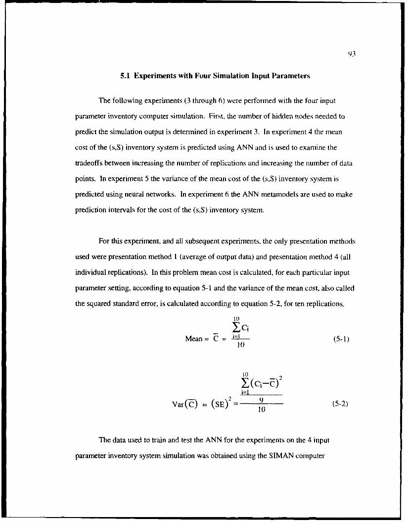
93
5.1 Experiments with Four Simulation Input Parameters
The following experiments (3 through 6) were performed with the four input
parameter inventory computer simulation. First, the number of hidden nodes needed to
predict the simulation output is determined in experiment 3. In experiment 4 the mean
cost of the (s,S) inventory system is predicted using ANN and is used to examine the
tradeoffs between increasing the number of replications and increasing the number of data
points. In experiment 5 the variance of the mean cost of the (s,S) inventory system is
predicted using neural networks. In experiment 6 the ANN metamodels are used to make
prediction intervals for the cost of the (s,S) inventory system.
For this experiment, and all subsequent experiments, the only presentation methods
used were presentation method 1 (average of output data) and presentation method 4 (all
individual replications). In this problem mean cost is calculated, for each particular input
parameter setting, according to equation 5-1 and the variance of the mean cost, also called
the squared standard error, is calculated according to equation 5-2, for ten replications.
10
jciMean= C = i=1 (5-1)
10
101o(Ci-O-C
i=l
Var(C) = (SE) 2 = 9 (5-2)10
The data used to train and test the ANN for the experiments on the 4 input
parameter inventory system simulation was obtained using the SIMAN computer

94
simulation programs given in Appendix B, Figures B I and B2. This simulation is identical
to the one used for the 2 input parameter inventory system except that the code was
modified to accommodate the larger number of input parameters. In these experiments a
reparameterization of the factor u was used to prevent having unreasonable combinations
of u and k. The reparameterization was to let w = k/u. In the 2 input parameter inventory
computer simulation the parameter k was always at the value $32 and the input parameter
u was always equal to the value $5 (and so the parameter w was 32/5, or 6.4).
The values of the four input parameters selected for training and testing neural
networks are shown in Table 9. Using ten values of s, ten values of d, five values of k and
five values of w, a total of 2,500 different combinations of input parameter values were
simulated ten times to obtain a total of 25,000 replications of training data. To examine
the tradeoffs of more data points versus additional replications, the training data was
divided into smaller non-disjoint sets. Table 9 shows several sets of values for each
parameter. The parameter s, has three sets of values, one set of size 2, one set of size 4
and one set of size 10. Similarly, d, k and w have three, four, and four sets of values
respectively. Thus, there are 144 (3x3x4x4) combinations of the different sets of values of
the input parameters. Table 10 shows the thirteen combinations of the sets of training
input parameter values that were considered in the experiments involving the 4 parameter
inventory system computer simulation. Each training set is a subset of any training set that
is below or to the right of it in Table 10. The one exception to this rule is training set J,
since it is a combination of training sets E and I, each of which contains the training set A,
with one of the two sets of training set A removed. Training set J was included to
examine the advantage of having detailed information about each input parameter without
the disadvantage of having very large amounts of data, as is the case with training set M.
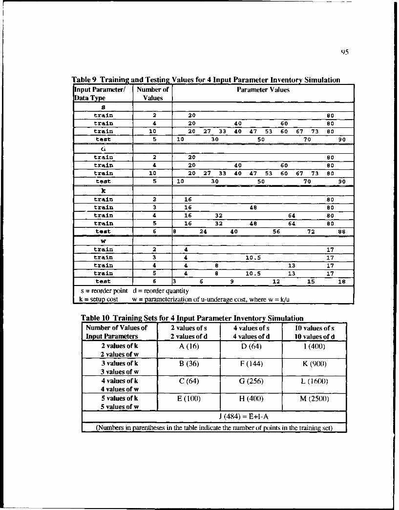
95
Table 9 Trainin and Testing Values for 4 Input Parameter Inventory SimulationInput Parameter/ Number of Parameter ValuesData Type Values
train 2 20 80train 4 20 40 60 80train 10 20 27 33 40 47 53 60 67 73 80test 5 10 30 50 70 90
train 2 20 80train 4 20 40 60 80train 10 20 27 33 40 47 53 60 67 73 80test 5 i0 30 50 70 90
ktrain 2 16 80train 3 16 48 80train 4 16 32 64 80train 5 16 32 48 64 80test 6 8 24 40 56 72 88
wtrain 2 4 17train 3 4 10.5 17train 4 4 8 13 17train 5 4 8 10.5 13 17test 6 3 6 9 12 15 18
s = reorder point d = reorder quantityk = setup cost w = parameterization of u-underage cost, where w = k/u
Table 10 Training Sets for 4 Input Parameter Inventory SimulationNumber of Values of 2 values of s 4 values of s 10 values of sInput Parameters 2 values of d 4 values of d 10 values of d
2 values of k A (16) D (64) 1(400)2 values of w3 values of k B (36) F (144) K (900)3 values of w4 values of k C (64) G (256) L (1600)4 values of w5 values of k E (100) H (400) M (2500)5 values of w
J (484) = E+I-A
(Numbers in parentheses in the table indicate the number of points in the training set)

96
Due to computer memory restrictions, the computer simulation program was run
in separate batches of 10 replications for the training data and 20 replications for the
testing data. To obtain independent replications, the random number streams shown in
Table B 1 were used for the different batches. To reproduce the computer simulation
results from SIMAN that were obtained in this research would require putting the input
data in an ASCII file in the same order that is shown in Table B2 in Appendix B. In Table
B2, all of the parameters begin with the smallest values. The first three parameters are
then held fixed and the values for parameter w are increased from the smallest to the
largest value. Then k is increased to its next highest value and the process is repeated to
the parameter w. This iterative process is repeated for all values of k, and then all values
of d and then all values of s. The process is repeated until all possible combinations are
achieved. The results of the first 90 data points for the 10 replications of the training set
are shown in Table B2. All of the data for the training sets was obtained by running the
simulation on training set M, and then dividing the results appropriately to form the other
training sets. An example of one of the training sets, specifically training set A, is shown
in Table 11 with the results of 10 replications of the computer simulation in terms of the
mean cost and the variance of the mean cost. Training set A is a 24 design which is the
standard full factorial design used in traditional response surface methods. Other more
sophisticated designs such as Box Behnkin and star point designs may be more
appropriate if optimization of the response surface is the goal. Training set F is shown in
Table B3 in Appendix B. Training set F is a 32 x 42 design. The data has been shuffled in
both Table 11 and Table B2 for ANN training purposes. M, the largest training set is a
102 x 52 design.
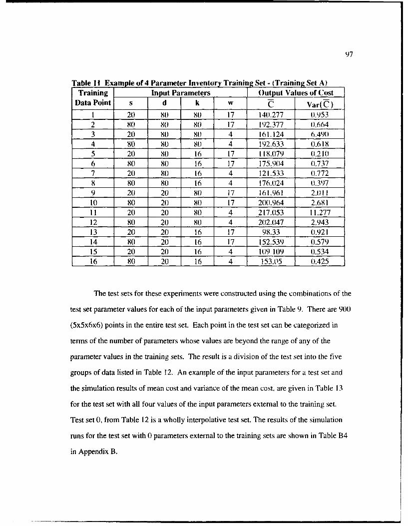
97
Table I1 Example of 4 Parameter Inventory Training Set - (Training Set A)Training Input Parameters (Output Values of Cost
Data Point s d k W C Var(C)
1 20 8O 8(0 17 14().277 0.9532 8() 80 80 17 192.377 0.6643 20 80 80 4 161.124 6.49014 80 80 80 4 192.633 0.6185 20 80 16 17 118.079 0.210(6 80 80 16 17 175.904 0.7377 20 80 16 4 121.533 0.7728 80 80 16 4 176.024 0.3979 20 20 80 17 161.961 2.01110 80 20 80 17 200.964 2.68111 20 20 80 4 217.053 11.27712 80 20 80 4 202.047 2.94313 20 20 16 17 98.33 0.92114 80 20 16 17 152.539 0.57915 20 20 16 4 1019 109 0.53416 80 20 16 4 153.05 0.425
The test sets for these experiments were constructed using the combinations of the
test set parameter values for each of the input parameters given in Table 9. There are 900
(5x5x6x6) points in the entire test set. Each point in the test set can be categorized in
terms of the number of parameters whose values are beyond the range of any of the
parameter values in the training sets. The result is a division of the test set into the five
groups of data listed in Table 12. An example of the input parameters for a test set and
the simulation results of mean cost and variance of the mean cost, are given in Table 13
for the test set with all four values of the input parameters external to the training set.
Test set 0, from Table 12 is a wholly interpolative test set. The results of the simulation
runs for the test set with 0 parameters external to the training sets are shown in Table B4
in Appendix B.

98
Table 12 Subdivisions of Test Set for 4 Parameter Inventory SimulationTest Set Number of Points in Test Set
(Number of parameters with valueexternal to training set values)
0 1441 3362 2923 1124 16
TOTAL 900
Table 13 Test Set with 4 External Values for 4 Parameter Inventory SimulationTesting Input Parameters Output Values of Cost
Data Point s d k w C Var(C)
1 10 10 8 3 115.13 2.062 10 10 8 18 87.92 0.713 10 10 88 3 518.13 100.114 10 10 88 18 219.77 6.195 10 90 8 3 118.09 0.626 10 90 8 18 111.30 0.517 10 90 88 3 216.72 19.208 10 90 88 18 143.18 1.579 90 10 8 3 151.95 0.3310 90 10 8 18 151.84 0.2511 90 10 88 3 230.04 0.5012 90 10 88 18 230.01 0.6213 90 90 8 3 188.05 0.4914 90 90 8 18 188.03 0.4915 90 90 88 3 207.83 0.6316 90 90 88 18 207.92 0.72
A traditional backpropagation training algorithm was used with a smoothing
factor and a unipolar sigmoidal transfer function as given in equation 3-1, with a training
tolerance of 0.02. For some prediction problems it is difficult for the ANN to achieve very
high values or very low values of the target output due to the undershoot phenomenon.

99
The default setting for the range of normalization of both the inputs and outputs in the
BrainMaker package is to use the minimum and maximum values observed in the training
data. In these experiments, the test data extends beyond the range of the training data
both in terms of inputs and outputs. Thus, for this research the range of normalization for
the input values was extended so that the minimum value was set at 10% of the range
lower than the minimum value of the train and test sets combined and the maximum value
was set at 10% of the range higher than the maximum value of the train and test sets
combined. For instance, for the input parameter s, the training set values had a minimum
of 20 and a maximum of 80, while the test set had a minimum of 10 and a maximum of 90.
Since the range of the combined train and test sets was 80 (90-10), BrainMaker used a
minimum value of 2 (10 -. 1 x 80) and a maximum value of 98 (90 +. 1 x 80) to scale the
input parameter s. The factor of 10% of the range beyond the minimum and maximum
values found in the test set was used after several trials using factors of 0%, 10%, and
20%. Similar trials were conducted to examine the factor to use for the output values
with the result that a 10% factor for adjusting the minimum and maximum of the mean
cost of operating the inventory system performed best. For predicting the variance of the
mean the factor used to adjust the range of the inputs remained at ± 10%, but the target
output used 10% lower than the minimum and 20% higher than the maximum since these
values yielded the best results. The remainder of these experiments used these
adjustments to the scaling factors for both the inputs and outputs of the ANN.
5.2 Experiment 3: Determining the Number of Hidden Nodes Needed toPredict the Simulation Output Measure
In this experiment the ANN architecture has four input nodes, two hidden layers
with a varying number of nodes, and a single output node. The objective of this

II K)
experiment was to determine how many nodes to use in the hidden layers. In this
experiment training sets A and M from Table i0 were used. These training sets were the
smallest and largest training sets, with 16 and 25(X) data points respectively. A total of Six
ANN were developed using these two training sets. Two of the ANN were developed
using the mean and the individual replications of training set A. Four of the ANN were
developed using the mean and the individual replications of training set M with two of
these ANN using shuffled data and two of them using unshuffled data.
Each of the networks in this experiment were trained for 50 epochs. The networks
were evaluated after each epoch, and the one which performed best on the training set was
saved as the final trained network. The average number of epochs required to reach the
minimum training error was 26.
The results on the test set in terms of Mean Absolute Error for the ANN trained on
the unshuffled data of set M are shown in Figure 32. As can be seen in the figure, the
best number of hidden nodes is five for both the averages and individual replications.
After this initial experiment, it was clear that the number of hidden nodes that would work
best for this data was between 2 and 10, and so, the succeeding examinations of the
number of hidden nodes was restricted to this range. After examining Figure 32, it
became apparent from the erratic behavior of networks trained on individual replications
that the ANN might have better and more stable performance if the training data was
shuffled for such a large training set. The results for data set A and the shuffled and
unshuffled data set M are provided in Figures 33 and 34. Figure 33 shows that all three of
the ANN trained on averages achieved the smallest MAE with five hidden nodes. Figure
34 shows that two out of three achieved the smallest MAE with five hidden nodes and the

other achieved the smallest MAE with four hidden nodes for the ANN trained on
individual replications. In addition, Figures 33 and 34 show that shuffling the data
improves the results by reducing the test set MAE and for the individual replications,
providing more stable performance. In all six cases good performance in terms of MAE
was achieved using five hidden nodes.
Based on these results the following ANN architecture is used in the remaining
experiments of predicting cost with the four input parameter inventory simulation: four
input nodes, two hidden layers of five nodes each, and a single output node. In addition,
since it was observed that the networks trained on data set A achieved their best level of
performance at 50 epochs, which was the maximum number of epochs for this experiment,
succeeding experiments increased the maximum number of epochs to 750.
PM] Averages 0 PN14 Repllcaflos
70
60
50 --
130
20 -
10 Smallest MAE
0 " I I I I I I
0 5 10 15 20 25 30 35 40 45 511
Number of Hidden Nodes
Figure 32 Results of Experiment 3 for Training Set M (Unshuffled Data)
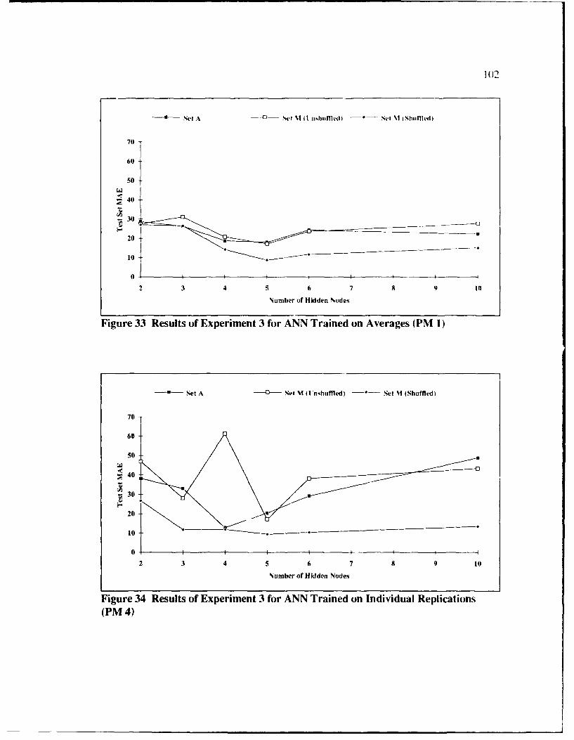
1 02
---- Set A S Ot %I I lshunfle)- Set %I IShuffled)
70
60
50
- 40
20 "
10
2 3 4 5 6 7 8 9 10
Number of Hidden Nodes
Figure 33 Results of Experiment 3 for ANN Trained on Averages (PM i)
0- Set A -C- Set M (Un-;hiffled) - S- Set M (Shuffled)
70 -
60
50 U
40
S30 f t
20
10 , _,
0 I I I -- ________________
2 3 4 5 6 7 8 9 10
Number of Hidden Nodes
Figure 34 Results of Experiment 3 for ANN Trained on Individual Replications(PM 4)
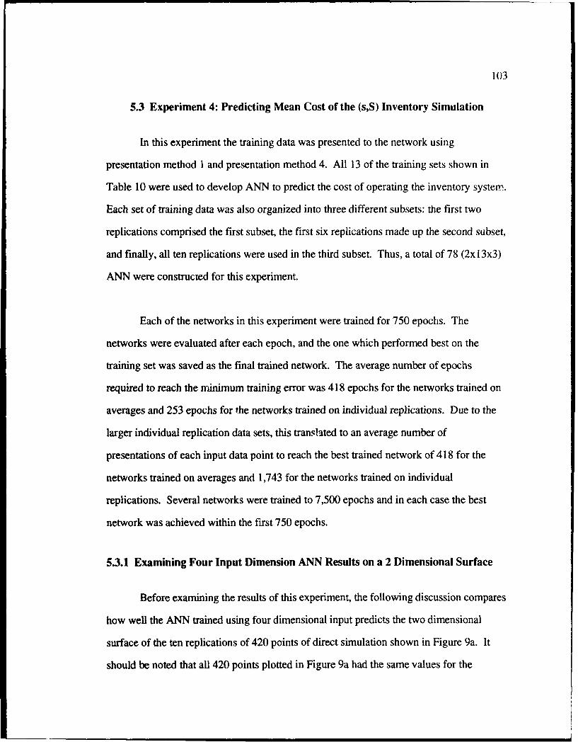
103
5.3 Experiment 4: Predicting Mean Cost of the (s,S) Inventory Simulation
In this experiment the training data was presented to the network using
presentation method 1 and presentation method 4. All 13 of the training sets shown in
Table 10 were used to develop ANN to predict the cost of operating the inventory system.
Each set of training data was also organized into three different subsets: the first two
replications comprised the first subset, the first six replications made up the second subset,
and finally, all ten replications were used in the third subset. Thus, a total of 78 (2x 13x3)
ANN were constructed for this experiment.
Each of the networks in this experiment were trained for 750 epochs. The
networks were evaluated after each epoch, and the one which performed best on the
training set was saved as the final trained network. The average number of epochs
required to reach the minimum training error was 418 epochs for the networks trained on
averages and 253 epochs for the networks trained on individual replications. Due to the
larger individual replication data sets, this translated to an average number of
presentations of each input data point to reach the best trained network of 418 for the
networks trained on averages and 1,743 for the networks trained on individual
replications. Several networks were trained to 7,500 epochs and in each case the best
network was achieved within the first 750 epochs.
5.3.1 Examining Four Input Dimension ANN Results on a 2 Dimensional Surface
Before examining the results of this experiment, the following discussion compares
how well the ANN trained using four dimensional input predicts the two dimensional
surface of the ten replications of 420 points of direct simulation shown in Figure 9a. It
should be noted that all 420 points plotted in Figure 9a had the same values for the

104
parameters k and w. The parameter k was set to 32 and the parameter w was set to 6.4.
The closest values in training set F to these settings are with k equal to 16 or 48 and w
equal to 8. Also there are only 16 different values in the (s,d) space in data set F. Table
14 compares the regression and ANN metamodels developed with the 36 points from
Chapter 4, shown in Figures 9b and 9c respectively, with the ANN metamodel developed
on the individual replications of training set F. Based on the three criteria of mean
absolute error, maximum absolute error and variance of error, the ANN developed on
training set F outperformed the regression developed with 36 points but did not do as well
as the ANN developed with 36 points. Figure 35 shows the predictions made by the
neural network developed for this experiment using the ten individual replications of data
set F. In spite of the sparseness of the training data and its dissimilarity with the test set,
the plot of predicted values for the ANN trained on the individual replications of training
set F appears to be reasonably close to the direct simulation plots of 420 points shown in
Figure 9a and appears to be at least as good as the plot constructed using the regression
on 36 points shown in Figure 9b.
Table 14 Comparison of Chapter 4 and Chapter 5 NetworksMetamodel Method Regression ANN ANN
Training Set Chapter 4 Chapter 4 Chapter 5Set B Set B Set F
Total Number of Training points 36 36 144Number of Different (s,d) Training 36 36 16
PointsMAE (Entire Test Set) 8.64 3.20 5.09
Maximum Error (Entire Test Set) 52.15 12.02 52.02Variance of Error (Entire Test Set) 33.71 4.64 32.66
MAE (Internal Points) 9.00 3.12 3.21Maximum Error (Internal Points) 23.33 8.29 9.57Variance of Error (Internal Points) 24.91 4.09 4.57
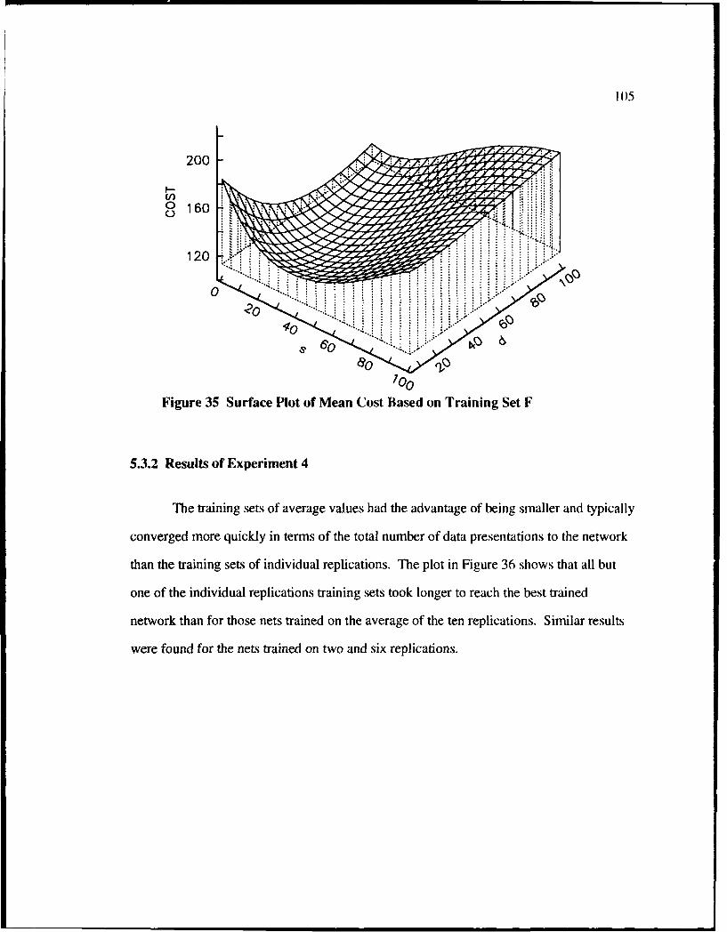
105
200
06
8 160120Sii0 (l ....
Figure 35 Surface Plot of Mean Cost Based on Training Set F
5.3.2 Results of Experiment 4
The training sets of average values had the advantage of being smaller and typically
converged more quickly in terms of the total number of data presentations to the network
than the training sets of individual replications. The plot in Figure 36 shows that all but
one of the individual replications training sets took longer to reach the best trained
network than for those nets trained on the average of the ten replications. Similar results
were found for the nets trained on two and six replications.
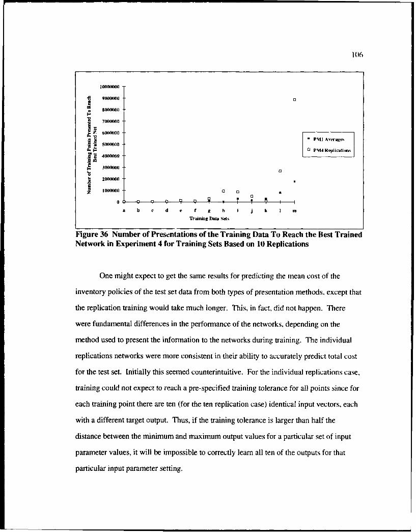
106
I80000000
9- 700)(1040
T PMJ Averages' 5000000
0 PM4 Replications4000000
S304000000
2000000
z I mm 0 0Z 0 Q P
a b c d e f g h i j k I InTraining Data Sets
Figure 36 Number of Presentations of the Training Data To Reach the Best TrainedNetwork in Experiment 4 for Training Sets Based on 10 Replications
One might expect to get the same results for predicting the mean cost of the
inventory policies of the test set data from both types of presentation methods, except that
the replication training would take much longer. This, in fact, did not happen. There
were fundamental differences in the performance of the networks, depending on the
method used to present the information to the networks during training. The individual
replications networks were more consistent in their ability to accurately predict total cost
for the test set. Initially this seemed counterintuitive. For the individual replications case,
training could not expect to reach a pre-specified training tolerance for all points since for
each training point there are ten (for the ten replication case) identical input vectors, each
with a different target output. Thus, if the training tolerance is larger than half the
distance between the minimum and maximum output values for a particular set of input
parameter values, it will be impossible to correctly learn all ten of the outputs for that
particular input parameter setting.

1 07
The output of the computer simulation for cost of the inventory system ranged in
value from 88 to 518. The average cost of all the points in the test set was 159. Figures
37, 38 and 39 show the networks trained on individual replications typically doing much
better than the networks trained on averages. All of the figures show the results in
alphabetical order of the training sets which are also in non-decreasing order of the size of
the training set. Figure 37 shows the results for the entire test set, while Figure 38 shows
the results for the test set consisting of all points with either zero or one value external to
the training sets and Figure 39 shows the results for all test points with either two, three or
four values external to the training sets.
As can be seen in Figure 37 only two of the networks, training sets E and K,
perform better with averages than with individual replications. Also as the number of
data points is increased the MAE decreases except for training sets E and 1. It is likely
that training sets E and I do poorer than networks trained on fewer data points because
they have too much information on some inputs. This can be seen by examining the data
sets in Table 10. Training set E might have too much information about the parameters k
and w. and not enough information about parameters s and d, while training set I might
have too much information about the parameters s and d and too little information about
parameters k and w.
The results in Figure 38 indicate that for a more interpolative test set, all training
sets with at least as many points as training set F (144 points) do better than those trained
on fewer than 144 points. For this test set, networks trained on averages only do better
than networks trained on individual replications for data sets E and K.
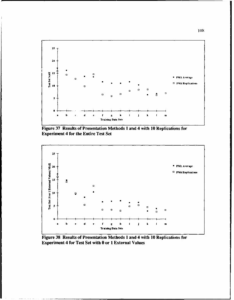
I0X
25
20
S15 oS* PMI Average
0 * • O PM4 Replicaliouls10 0
0 0 (30
0
0 I I I I i I I I I
a b C d e f g h i j k I In
Training Data Sets
Figure 37 Results of Presentation Methods I and 4 with 10 Replications forExperiment 4 for the Entire Test Set
25 -
20 - PMJ Average
0 PM4 Replications
15
5 0 0110 1
5o oU
a b c d e f g h I k I m
T~raining Data Sets
Figure 38 Results of Presentation Methods I and 4 with 10 Replications forExperiment 4 for Test Set with 0 or I External Values
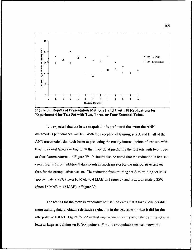
109
251
20
• •" PM1I Avs•age
> PM4 Repications~15 O •
0
0 0r 010I 0 0
0~
0 I I I I I I I I I
a b c d e r a h i j k I m
Training Data Sets
Figure 39 Results of Presentation Methods I and 4 with 10 Replications forExperiment 4 for Test Set with Two, Three, or Four External Values
It is expected that the less extrapolation is performed the better the ANN
metamodels performance will be. With the exception of training sets A and B, all of the
ANN metamodels do much better at predicting the mostly internal points of test sets with
0 or 1 external factors in Figure 38 than they do at predicting the test sets with two, three
or four factors external in Figure 39. It should also be noted that the reduction in test set
error resulting from additional data points is much greater for the interpolative test set
than for the extrapolative test set. The reduction from training set A to training set M is
approximately 75% (from 16 MAE to 4 MAE) in Figure 38 and is approximately 25%
(from 16 MAE to 12 MAE) in Figure 39.
The results for the more extrapolative test set indicates that it takes considerable
more training data to obtain a definitive reduction in the test set error than it did for the
interpolative test set. Figure 39 shows that improvement occurs when the training set is at
least as large as training set K (900 points). For this extrapolative test set, networks

I10
trained on averages only do better than networks trained on individual replications for data
set K.
For all of the test sets it appears from Figures 38 and 39 that networks trained on
very little data (Training Sets A, B and C) or on a lot of data (Training Sets L or M) are
not much different for the two data presentation methods. However, for the training sets
from D through K there does appear to be a difference between training on averages and
training on individual replications.
The result of increasing the number of replications at each point is shown in
Figures 40 through 43. Figures 40 and 41 show the results for presentation method 1
(averages) with the entire test set and the test set with 0 factors external, respectively.
Similarly, Figures 42 and 43 show the results for presentation method 4 (individual
replications). All four of the figures demonstrate that training neural networks is a
stochastic versus a deterministic process. Figures 40 and 41 show that there is not much
benefit to increasing the number of replications when training on the averages. Figures 42
and 43 indicate that there is a slight benefit to increasing the number of replications when
training the ANN is based on individual replications. For other problems the effect of
additional replications could be much more pronounced. These results indicate that for
this problem there is much more variability between the input data points than there is
within the replications performed at a particular data point. It should be noted that the
error on the purely interpolative test set as shown in Figures 41 and 43 is quite small for
both presentation methods once sufficient data points (at least 144 points with data set F)
are provided as the training set.
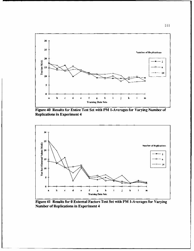
310
25Number of Replications
20----
15 -s--o----6
a b c d e f g h I j k I m
Training Data Sets
Figure 40 Results for Entire Test Set with PM I-Averages for Varying Number ofReplications in Experiment 4
S~Number of Replicationas
~j22
S15 " "--0" 6
C]
01
S10"SIlt-
5
0 t I I I I I I I I Ia b c d e f g h I j k I m
Training Data Sets
Figure 41 Results for 0 External Factors Test Set with PM I-Averages for VaryingNumber of Replications in Experiment 4
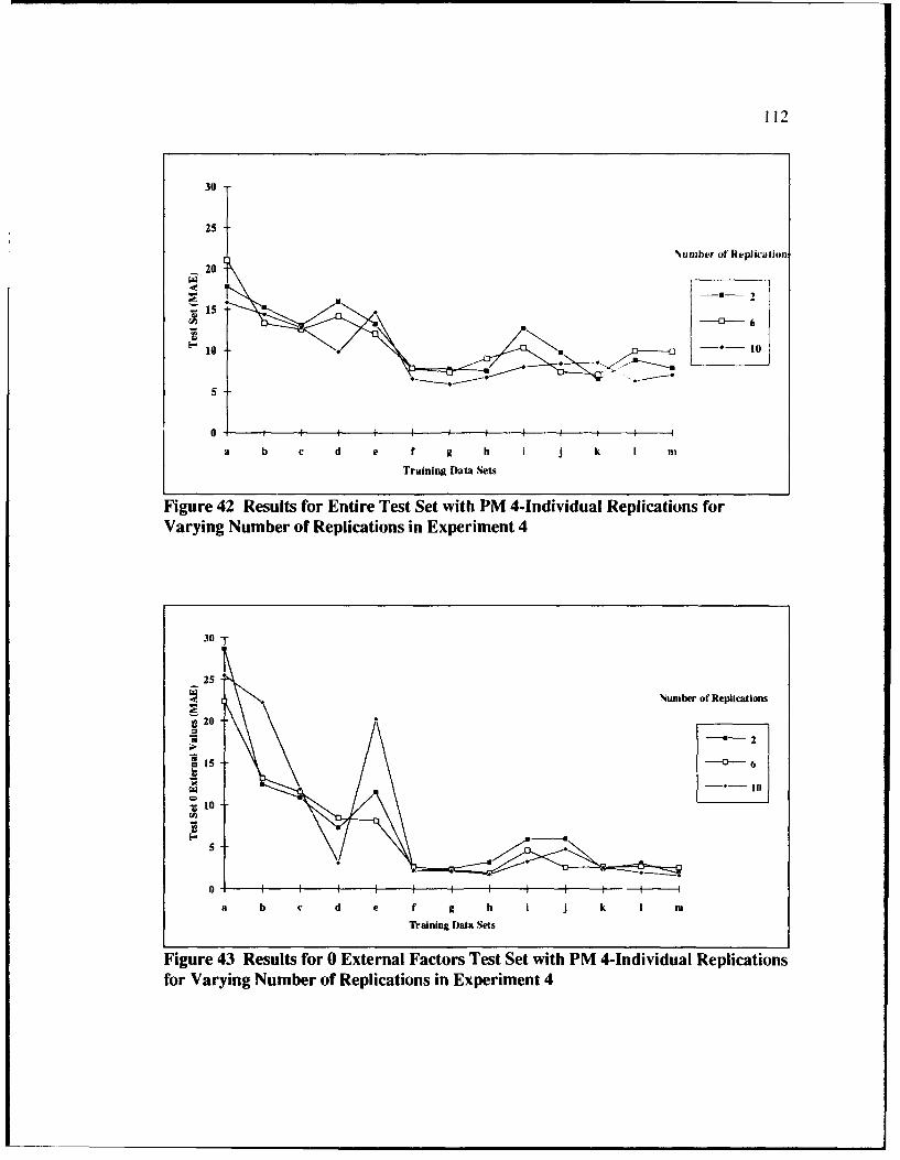
112
30
25
Number o~f Rteplication,
20
- - 6
10 10
a b c d e f 9 h i j k I m
Training Data Sets
Figure 42 Results for Entire Test Set with PM 4-Individual Replications forVarying Number of Replications in Experiment 4
30 T
__25
Number of Replications
220
i15 -~-6
-10
I.-.-..-
5
0I i It I I I I
a b c d e f g h i j k I m
Training Data Sets
Figure 43 Results for 0 External Factors Test Set with PM 4-Individual Replicationsfor Varying Number of Replications in Experiment 4
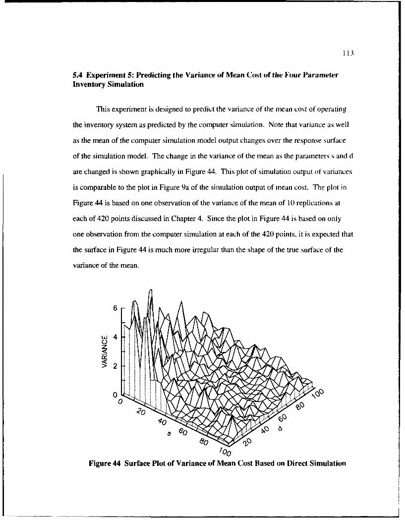
113
5.4 Experiment 5: Predicting the Variance of Mean Cost of the Four ParameterInventory Simulation
This experiment is designed to predict the variance of the mean cost of operating
the inventory system as predicted by the computer simulation. Note that variance as well
as the mean of the computer simulation model output changes over the response surface
of the simulation model. The change in the variance of the mean as the parameters s and d
are changed is shown graphically in Figure 44. This plot of simulation output of variances
is comparable to the plot in Figure 9a of the simulation output of mean cost. The plot in
Figure 44 is based on one observation of the variance of the mean of 10 replications at
each of 420 points discussed in Chapter 4. Since the plot in Figure 44 is based on only
one observation from the computer simulation at each of the 420 points, it is expected that
the surface in Figure 44 is much more irregular than the shape of the true surface of the
variance of the mean.
6
w 4
z
F 20
10oFigure 44 Surface Plot of Variance of Mean Cost Based on Direct Simulation
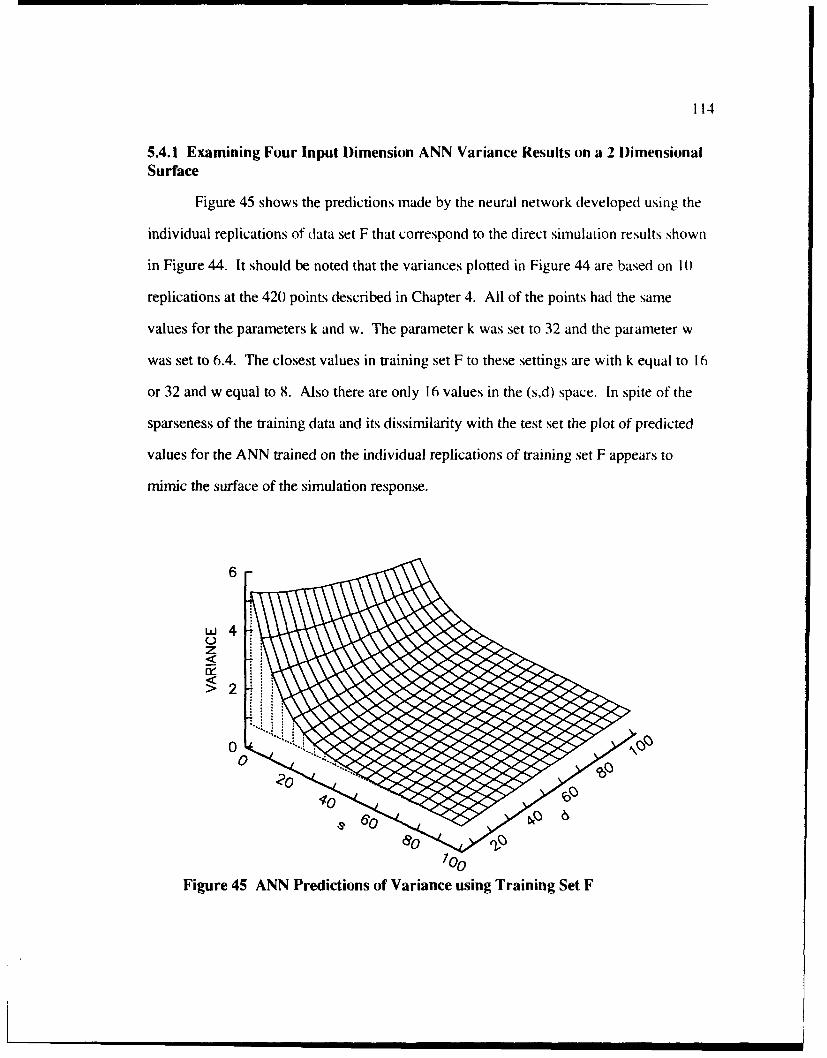
114
5.4.1 Examining Four Input Dimension ANN Variance Results on a 2 DimensionalSurface
Figure 45 shows the predictions made by the neural network developed using the
individual replications of data set F that correspond to the direct simulation results shown
in Figure 44. It should be noted that the variances plotted in Figure 44 are based on 10
replications at the 420 points described in Chapter 4. All of the points had the same
values for the parameters k and w. The parameter k was set to 32 and the paiameter w
was set to 6.4. The closest values in training set F to these settings are with k equal to 16
or 32 and w equal to 8. Also there are only 16 values in the (s,d) space. In spite of the
sparseness of the training data and its dissimilarity with the test set the plot of predicted
values for the ANN trained on the individual replications of training set F appears to
mimic the surface of the simulation response.
6
Fur 4'11Oo
Figure 45 ANN Predictions of Variance using Training Set F
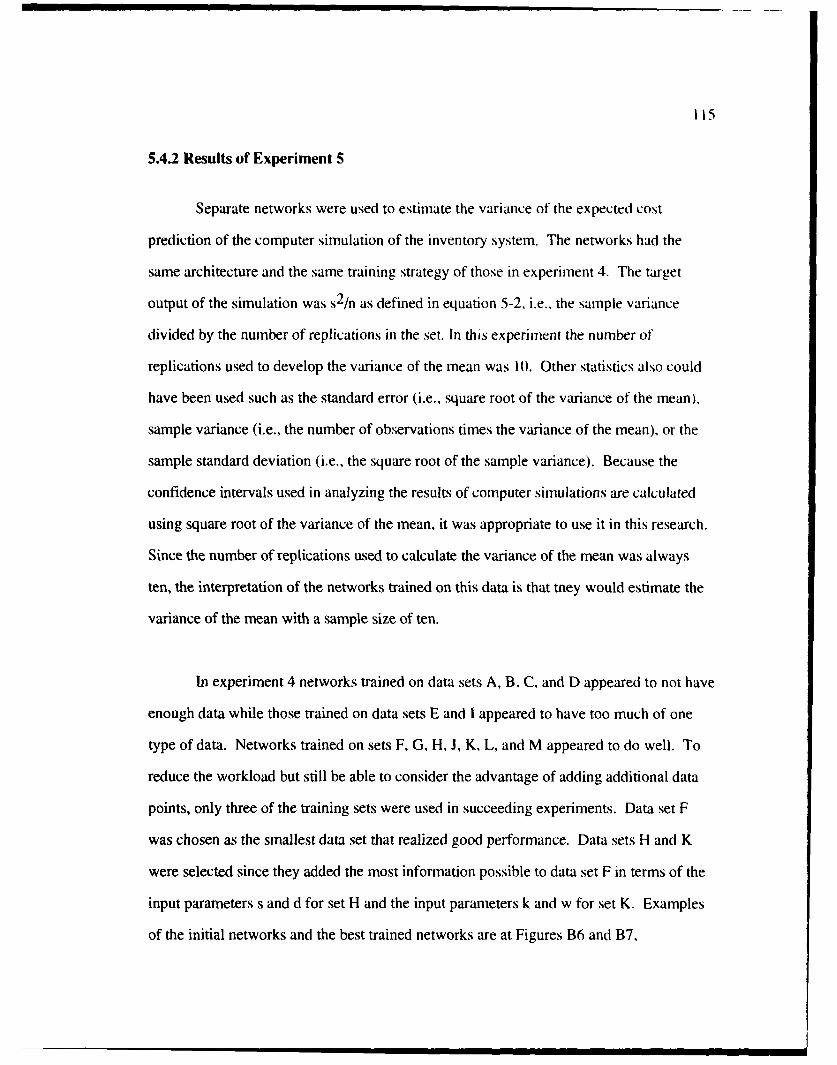
115
5.4.2 Results of Experiment 5
Separate networks were used to estimate the variance of the expected cost
prediction of the computer simulation of the inventory system. The networks had the
same architecture and the same training strategy of those in experiment 4. The target
output of the simulation was s2 /n as defined in equation 5-2, i.e., the sample variance
divided by the number of replications in the set. In this experiment the number of
replications used to develop the variance of the mean was 10. Other statistics also could
have been used such as the standard error (i.e., square root of the variance of the mean),
sample variance (i.e., the number of observations times the variance of the mean), or the
sample standard deviation (i.e., the square root of the sample variance). Because the
confidence intervals used in analyzing the results of computer simulations are calculated
using square root of the variance of the mean, it was appropriate to use it in this research.
Since the number of replications used to calculate the variance of the mean was always
ten, the interpretation of the networks trained on this data is that tney would estimate the
variance of the mean with a sample size of ten.
In experiment 4 networks trained on data sets A, B, C, and D appeared to not have
enough data while those trained on data sets E and 1 appeared to have too much of one
type of data. Networks trained on sets F, G, H, J, K, L, and M appeared to do well. To
reduce the workload but still be able to consider the advantage of adding additional data
points, only three of the training sets were used in succeeding experiments. Data set F
was chosen as the smallest data set that realized good performance. Data sets H and K
were selected since they added the most information possible to data set F in terms of the
input parameters s and d for set H and the input parameters k and w for set K. Examples
of the initial networks and the best trained networks are at Figures B6 and B7,

116
res,,pectively. An example of the data (Set FI used to train the networks on the variance of
the mean is shown in Table B3 under the column Var(C ). The data used to tet the ANN
is described in Table 12. The test set values for the variance of the mean were obtained by
averaging the variance of the mean of ten different sets of ten replications each. The
variance of the mean of each set of ten replications was calculated using equation 5-2.
Two uf the test sets described in Table 12 are provided in this dissertation. The simulation
results for the te',' set with 0 factors external is at Table B4 under the column Var(C ).
The simulation results for the test set with 4 factors external is at Table 13 under the
column Var(C).
The range of the variance of the mean was from 0.03 to 48.93 with an average
value over the 900 points of the entire test set of 1.64. After experimenting with various
combinations of distances to extend the scaling range on the outputs, the best combination
found was 10% of the range lower than the minimum value and 20% of the range higher
than the maximum value.
Each of the networks in this experiment were trained for 750 epochs. The
networks were evaluated after each epoch, and the one which performed best on the
training set was saved as the fin;Ai trained network. The number of epochs required to
reach the minimum training error for each of the training sets is shown in Table 15. The
average number of epochs required to reach the minimum training error was 424 epochs.
The results of training and testing the three networks on the variance of the mean
are shown in Table 15. From these results it is apparent that there is not much gained by
increasing the number of data points from training set F to either training set H or training
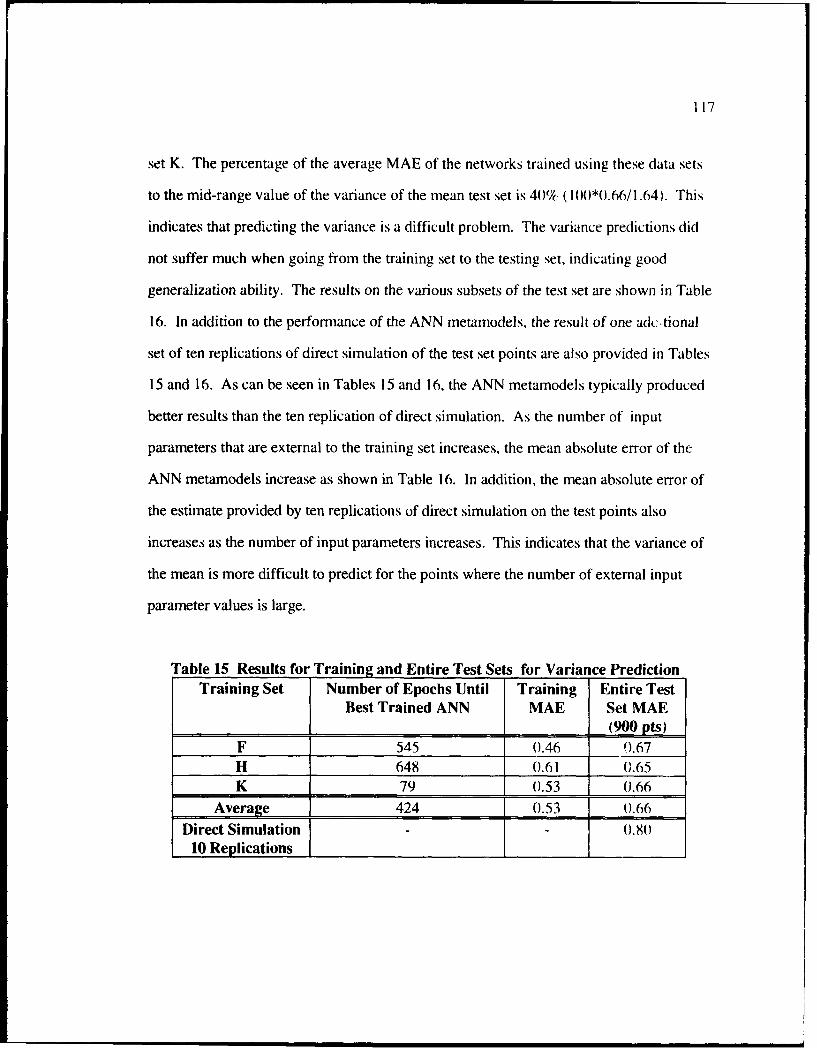
117
set K. The percentage of the average MAE of the networks trained using these data sets
to the mid-range value of the variance of the mean test set is 40% (100*0.66/1.64). This
indicates that predicting the variance is a difficult problem. The variance predictions did
not suffer much when going from the training set to the testing set, indicating good
generalization ability. The results on the various subsets of the test set are shown in Table
16. In addition to the performance of the ANN metamodels, the result of one adc.tional
set of ten replications of direct simulation of the test set points are also provided in Tables
15 and 16. As can be seen in Tables 15 and 16, the ANN metamodels typically produced
better results than the ten replication of direct simulation. As the number of input
parameters that are external to the training set increases, the mean absolute error of the
ANN metamodels increase as shown in Table 16. In addition, the mean absolute error of
the estimate provided by ten replications of direct simulation on the test points also
increases as the number of input parameters increases. This indicates that the variance of
the mean is more difficult to predict for the points where the number of external input
parameter values is large.
Table 15 Results for Training and Entire Test Sets for Variance PredictionTraining Set Number of Epochs Until Training Entire Test
Best Trained ANN MAE Set MAE(900 pts)
F 545 0.46 0.67H 648 0.61 0.65K 79 (0.53 0.66
Average 424 0.53 J 0.66
Direct Simulation - - .8010 Replications _

Ilx
Table 16 MAE Results for Test Subsets for Variance PredictionTraining Set Test Set Number of Factors External
0 1 2 3 4
F 0.23 0.40 0.71 1.67 2.63H 0.15 0.32 0.69 1.89 2.66K 0.25 0.35 0.79 1.67 1.73
Average 0.21 0.35 0.73 1.75 2.34Direct Simulation 0.27 0.44 0.76 1.43 9.63of 10 Replications I I I
For comparing the difficulty of developing metamodels of the mean to developing
metamodels of the variance of the mean, the results for predicting the cost with the same
training sets that were used to predict the variance of the mean are shown in Table 17. As
can be seen by comparing the results from Table 15 and 17 there is much more variability
between the MAE of the different ANN metamodels for predicting cost than for predicting
variance. While the size of the error is larger for predicting cost than for predicting
variance the percentage of the error to the average value in the test set is much smaller for
the cost metamodels than for the variance of the mean metamodels. The average MAE of
the networks trained using these data sets to the average value of the cost test set is
5.3 1% (100*8.45/159). The results for the subsets of the test set shown in Table 18
indicate that the direct simulation of ten replications does better than the ANN
metamodels especially as the number of external parameters in the test set increase. This
reinforces the previous observations that ANN metamodels perform interpolation fairly
well but may not extrapolate very well.
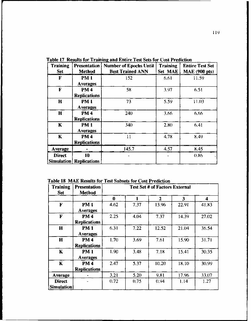
119
Table 17 Results for Training and Entire Test Sets for Cost PredictionTraining Presentation Number of Epochs Until Training Entire Test Set
Set Method Best Trained ANN I Set MAE MAE (9 00 pts)F PM 1 152 6.61 11.59
AveragesF PM 4 58 3.97 6.51
Replications
H PM 1 73 5.59 11.03Averages
H PM 4 241 3.66 6.66Replications
K PM 1 34( 2.80 6.41Averages
K PM 4 11 4.78 8.49Replications
Average 145.7 4.57 8.45Direct 10 - - 0.86
Simulation Replications I
Table 18 MAE Results for Test Subsets for Cost PredictionTraining Presentation Test Set # of Factors External
Set Method0 1 2 3 4
F PM 1 4.62 7.37 13.96 22.91 41.83Averages
F PM 4 2.25 4.04 7.37 14.39 27.02Replications
H PM 1 6.31 7.22 12.52 21.04 36.54Averages
H PM 4 1.70 3.69 7.61 15.90 31.71Replications
K PM 1 1.90 3.48 7.18 15.41 30.35Averages
K PM 4 2.47 5.37 10.20 18.10 30.99Replications
Average 3.21 5.20 9.81 17.96 33.07Direct -0.72 (0.75 0.94 1.14 1.27
Simulation I

120
5.5 Experiment 6: Comparing Prediction Intervals from Direct Simulation withthose Developed from ANN Approximations of the Computer Simulation
To evaluate the overall perfo-rmance of the neural network metamodels, the neural
network estimates of total cost and of the variance of total cost were combined using
equation 5-3 to form neural prediction intervals. Prediction intervals are similar to
confidence intervals but instead of predicting how often the true mean would fall in an
interval they predict how often an observation from the distribution would fall in the
interval. While prediction intervals are not used by the simulation community as often as
confidence intervals are used, they do provide an efficient means of comparing the
accuracy of the intervals developed by the ANN with the intervals developed by direct
simulation. The prediction intervals were constructed for each of the 900 test vectors
using the neural network predictions for the mean and variance of the mean. In addition
similar prediction intervals were constructed directly from 10 additional simulation
replications made at each test vector.
Prediction Interval '/2 ×Var()xl 0 = t 9 1_/xs (5-3)
(Note that s is the estimate of the standard deviation of cost.)
The simulation generated prediction intervals were compared with the neural
generated prediction intervals by using 100 additional simulation replications at each test
point and counting the number of these which fell into each interval. If the simulation
prediction interval or the neural prediction interval were perfect, then a number of
replications equal to the confidence level would fall within the interval, with equal
numbers falling on either side of the interval. For example, an 90% prediction interval (at=
0.05) should include 90 of the 100 replications with 5 replications falling above the
interval and 5 replications falling below the interval, for each test point.

121
The results for the estimation of the variance of the mean cost for training sets F,
H and K are given in Table 14 and the results for the estimation of the mean cost for the
same training sets are given in Table 15. While the neural network prediction intervals
were not :curate as those generated by the simulation, in many instances they were
quite rc,, , able. The goodness of the prediction intervals was more dependent on the
quality of the neural prediction of total cost, than that of the prediction of variance for this
problem. The networks which did poorly for estimation of total cost, also made poor
prediction intervals, as might be expected. In general, these were the networks trained on
mean value, rather than individual replications. Therefore, it is critical that the networks
estimating both the mean value of the simulation and the variance be validated and verified
as strongly as possible, before proceeding to building prediction intervals. Table 19 shows
the results of the 100 replications averaged over the 144 points of the interpolative test set
(no external values) for 90%, 95% and 99% confidence levels.
Table 19 Prediction Interval Results for Test Set 0Train Conf. ANN_-_Replications Neural Nets - Mean Simulation Intervals
Set Level Low Interval High Low Interval High Lw Interval High
F 90 1.4 83.0 15.6 39.9 57.4 2.7 5.6 88.9 5,5F 95 0.4 91.3 8.3 29.3 69.5 1.2 2.7 94.3 3.0F 99 0.0 98.9 1.1 10.8 89.1 0.1 0.6 98.8 0.7H 90 4.6 82.3 13.1 64.0 33.8 2.2 5.6 88.9 5.5H 95 2.1 90.6 7.3 55.8 43.0 1.2 2.7 94.3 3.0H 99 0.2 98.6 1.2 34.6 65.2 0.2 0.6 98.8 0.7K 90 12.1 83.2 4.7 3.0 89.2 7.8 5.6 88.9 5.5K 95 6.0 91.5 2.5 1.2 95.6 3.2 2.7 94.3 3.0K 99 0.7 99.0 0.3 0.1 99.7 0.2 0.6 98.8 0.7
Two further observations from Table 19 can be made. First, the neural network
intervals are not likely to be correctly centered. That is, they are biased upwards or
downwards. Since the prediction intervals themselves are symmetric, this is an effect of
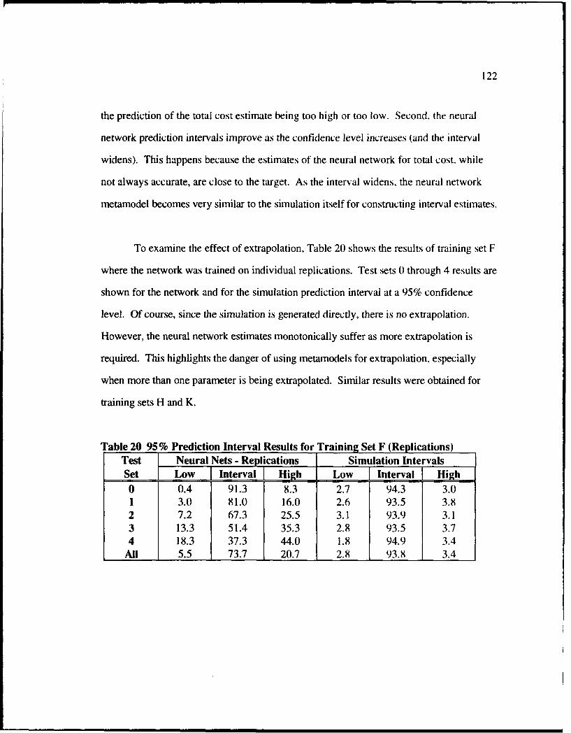
122
the prediction of the total cost estimate being too high or too low. Second, the neural
network prediction intervals improve as the confidence level increases (and the interval
widens). This happens because the estimates of the neural network for total cost, while
not always accurate, are close to the target. As the interval widens, the neural network
metamodel becomes very similar to the simulation itself for constructing interval estimates.
To examine the effect of extrapolation, Table 20 shows the results of training set F
where the network was trained on individual replications. Test sets 0 through 4 results are
shown for the network and for the simulation prediction interval at a 95% confidence
level. Of course, since the simulation is generated directly, there is no extrapolation.
However, the neural network estimates monotonically suffer as more extrapolation is
required. This highlights the danger of using metamodels for extrapolation, especially
when more than one parameter is being extrapolated. Similar results were obtained for
training sets H and K.
Table 20 95% Prediction Interval Results for Training Set F (Replications)Test Neural Nets - Replications Simulation IntervalsSet Low Interval High Low Interval High
0 0.4 91.3 8.3 2.7 94.3 3.01 3.0 81.0 16.0 2.6 93.5 3.82 7.2 67.3 25.5 3.1 93.9 3.13 13.3 51.4 35.3 2.8 93.5 3.74 18.3 37.3 44.0 1.8 94.9 3.4
All 5.5 73.7 20.7 2.8 93.8 3.4

123
5.6 Synopsis of Conclusions from Experiments 3 through 6
It has been shown that a combined expected value/variance neural network
metamodel approach can be successful for establishing prediction intervals of discrete
event simulations. For this problem, training on the individual replications yielded more
precise predictions of expected values at the expense of longer training times (the size of
the training set for replications is ten times the size of the training set for means). It
probably would be possible to improve the variance metamodel by using sets of
replications for estimating the variance at each point; i.e., instead of a single estimate of
variance based on ten replications, one could take ten estimates based on 100 replications
(10 sets of 10). This approach would be considerably more expensive in terms of training
data requirements. Another approach that would not require as much training data is the
technique used in cross validation with test sets. As an example, generate 11 observations
and form all 11 possible subsets of size ten. Then determine the variance of each subset
and take the average value of the 11 variances of the subsets and use the average value of
the variances as the training data. A third approach would be to use more than one sample
size when developing the variance of the mean estimates. For example, generate 10
observations, and form all possible subsets of size 2, 3, 4,..., 10. Calculate the sample
variance of the mean for each of the subsets and then determine the average variance of
the mean for all subsets of the same size. If the average variance of the mean is similar
regardless of how many observations are in the sample, then use all of the data with the
original input parameters. If the average variance of the mean is quite different as one
changes the size of the sample, then the ANN would require an additional input, the size
of the sample used to calculate the variance of the mean. While this study was promising
clearly more work needs to be done on the trade-offs of precision and computational
effort when using neural networks as simulation metamodels.

124
In most cases the networks trained on averages performed much worse than their
replication counterparts. One conjecture as to why this happens is the effect of extreme
values. The calculated mean of the ten replications gives equal probability mass (0. 10) to
each replication. A replication representing an extrerne outcorne will strongly influence
the mean. The neural network does not necessarily min-iic rnean value beh-tvior. Gradient
descent (the backpropagation training algorithm) will move to the error surface location
which best suits the majority of the observations. The network may find weights which
better reflect the true mean by ignoring (or partly ignoring) the extrerne replication.
Certainly, replication training gives more information to the network, since none of the
simulation data is discarded. In fact it is an open research issue as to what neural
networks are attempting to learn when being trained on individual replications. One
interesting question to consider is whether networks trained on individual replications are
learning the mean, a trimmed mean, or the median.
An additional intriguing idea is to train separate networks to learn the quantiles of
simulation output rather than just the mean and variance of the mean. In this way a farridy
of ANN could be used to produce the distribution of the simulation output as opposed to
just producing the mean and variance of the simulation output. If it is possible to obtain
the distribution of the simulation output then it would be possible to capture the stochastic
nature of the simulation. This would be important if one were trying to replace a
computationally expensive module in a larger computer simulation in which the stochastic
behavior of the module is necessary for interaction with the rest of the larger simulation.

125
5.7 Summary
Four experiments using a four input parameter version of the (s.S)
inventory simulation were examined in this chapter. The experiments included
determining the number of hidden nodes to use in predicting the cost of the
inventory system, predicting the mean cost of the inventory system, predicting the
variance of the mean cost of the inventory system and building prediction intervals
for the mean cost of the inventory system. The results of determining the number
of hidden nodes shows that there tends to be a pattern to the mean absolute error
of the test set as the number of hidden nodes in each of the two hidden layers is
increased. The pattern of the test set MAE is that it starts to decrease until hitting
a minimum value and then continues to increase. This might initially seem
counterintuitive since more learning capability is added to the ANN as the number
of hidden nodes is increased and so one might expect the error to continually
decrease. While the error for the training set does tend to continue to decrease as
the number of hidden nodes is increased the inherent danger in doing so is that the
network is memorizing the training set data and then does a poor job at
generalizing to points that it has not been trained on. Thus, the result of this
experiment shows that with too few hidden nodes the ANN doesn't have enough
learning power and that if it has too many hidden nodes the ANN can learn the
training data too well in a process typically termed overfitting the data. This result
indicates the need to have a procedure for finding the best number of hidden nodes
to use in developing an ANN metamodel of a computer simulation.
The remaining experiments show that ANN procedure extends quite easily
from two input parameters to four input parameters and as is shown visually is
-- -- --.. ,,.,-- .~ n n Nmmmmmm mmmmmmmm m M N

126
Section 5.3.1 without much lost in terms of accuracy. Neural network metamodels
were built for both the mean cost and the variance of the mean cost. As was
observed in Chapter 4, the networks constructed using individual replications
typically produce better metamodels than those trained on averages. The ANN
metamodels of mean and variance are used to form prediction intervals, which are
compared to those formed by direct simulation on the test set.

127
6.0 BASELINE ANN METAMODEL APPROACH
The ANN approach to approximating discrete event computer simulations,
developed as a result of the experiments conducted on the inventory simulation in
Chapters 4 and 5, is specified in this chapter. This is a necessary step in this fledgling area
of research since there is no one "right" approach to an approximation or estimation
problem using ANN.
6.1 Description of the Baseline ANN Metamodel Approach
The baseline ANN metamodel approach has three main phases. These phases are:
to decide upon and obtain simulation input and output data; to develop the ANN
metamodels; and to evaluate the effectiveness of the ANN metamodels in order to
determine whether additional da - needed.
6.1.1 Phase 1 of the Baseline ANN Metamodel Approach
To determine and obtain simulation input and output data, the following steps are
carried out in this phase of the metamodel approach. The user of the system should be
involved in this phase in as much as the selection of which inputs and outputs are
important depends on the user.
1. Identify the outputs of the simulation that are of interest.
2. Determine which controllable and uncontrollable inputs would have an effect on
the outputs of interest. Select the inputs to be used in building the metamodel.

128
3. Determine the minimum and maximum values that are of interest for each
selected input.
4. Determine how many values between the minimum and maximum values for
each selected input are needed for developing the ANN metamodels. If it is only
necessary to establish a linear approximation of the relationship between the input
parameter and the output measure, then no additional points other than the minimum and
maximum values would be needed. If more complicated approximations are desired (e.g.,
second-order, third-order or higher) then additional values will have to be included.
5. Identify the values between the minimum and maximum values for each
selected input that are needed for testing the ANN metamodels.
6. Calculate the total number of points in the selected input parameter space, for
both training and testing the ANN metamodels, by determining the number of possible
combinations of input parameter values in the training set and the number of possible
combinations of the input parameter values in the testing sets.
7. Determine the desired precision of the outputs.
8. Estimate the number of replications needed to achieve the desired precision for
each point in the selected input parameter space.

129
9. Calculate the total number of replications required to be run on the simulation
based on the total number of points in the selected input parameter space and the
estimated number of replications required for each point.
10. Estimate the time and computer memory requirements for making the
computer simulation runs. If the requirements are unreasonable, then repeat steps I
through 9 until they are reasonable.
11. Run the simulation to obtain the results for the training and testing sets.
12. Perform post-simulation processing to obtain sample averages and variances
for each point in the selected input parameter spaces for each of the desired outputs. This
step could be eliminated if comparisons between alternative points are not a requirement
and the only information desired is an estimate of the output measures for different input
parameter settings.
6.1.2 Phase H of the Baseline ANN Metamodel Approach
ANN metamodels for each of the desired outputs are developed in this phase of
the approach. If time, or computing resources are limited, then averages and sample
variances should be used as the target output. If accuracy of the metamodel is very
important, then the individual replications and sample variances should be used. If the
only information desired is an accurate tool for estimating the output measures for various
input parameter settings, then the individual replication information should be used. The
following steps are performed for each of the different output measures that are to be
approximated by a metamodel.

13)
1. Randomize the cider of the data in the training set so the different values of the
input parameters are spread evenly throughout the file of the training data.
2. Select the minimum and maximum values for scaling the inputs and outputs to
the ANN training package. A rule of thumb is to use 10% of the range less than the
minimum value of the training and testing sets and 10% of the range more than the
maximum value of the training and testing sets. In short, the values used for scaling
should be set to + 10% beyond the range of the training and testing sets.
3. Select an initial setting for the maximum number of epochs for learning, where
an epoch is defined as one pass through the training data. In this research the maximum
number of epochs varied from 50 to 5,000. Select the training tolerance small enough to
ensure the networks do not terminate prior to reaching the maximum numoer of runs.
4. Initialize the ANN training architecture as follows:
Input layer having one node for each input parameter.
Two hidden layers each with two nodes. If there is some reason to believe
that the relationships in the data are too complex to be learned with only two nodes in
each hidden layer then the initial number of hidden nodes could be increased.
Output layer having one node.
5. Perform "best net training" using standard backpropagatirn with a smoothing
factor. Best net training simply means that at the end of each epoch the network is
evaluated on the training set and the results of the evaluation are written tc a file. If the
training is being done on individual replications theni the testing could be done on the

131
average values of the training set to prevent unnecessary computations. At the conclusion
of training, the results file is examined to determine at which epoch the smallest mean
absolute error (MAE) occurred for the training set. Training to this epoch results in the
"best trained net." Compare the number of epochs to the "best trained net" to the
maximum number of epochs training termination criterion. If the two numbers are close,
then the network might benefit from additional training and so the maximum number of
epochs should be increased and this step should be repeated.
6. Increase the number of nodes in each hidden layer by one and return to Step 5.
Stop this process when no improvement is observed in the test set over previous
iterations. If the test set is very small, an alternative is to stop the process when no
improvement is observed over previous iterations of a weighted average of the training
and test sets mean absolute error.
7. Retrain the initial network in a "learning only" mode, (i.e., no data is written to
results files) until reaching the "best trained net" epoch at which time it is saved as the
"best trained net." This step is necessary because the weights after each epoch are not
stored. This step is much faster than the "learn and evaluate" portion of the training
conducted in Step 5.
6.1.3 Phase 11 of the Baseline ANN Metamodel Approach
To evaluate effectiveness of the ANN metamodels and to determine if additional
training data is needed, the following steps are taken in this phase for each of the different
output measures.

132
1. Evaluate the resulting networks in terms of mean absolute error and maximum
absolute error for the training and testing sets. If any of these measures exceed the desired
performance, then additional training data will be required in order to make the ANN
model attain the desired accuracy.
2. Construct confidence intervals and/or prediction intervals using the prediction
for the mean and the prediction for the variance of the mean. The validity of the
prediction intervals can be checked by obtaining additional independent observations from
the simulation and observing the number of observations that fall to the left, inside, or to
the right of the prediction intervals.
3. Conduct non-parametric tests on the ranked observations of the simulation data
compared to the ANN predictions for both the training and testing sets. If the ANN
metamodels do not perform well in comparison to the direct simulation then additional
training data will be required.
6.2 Assumptions of the Baseline ANN Metamodel Approach
There are several assumptions that were made in developing the ANN approach to
approximating stochastic discrete event computer simulations. These assumptions are
listed below:
1. The simulation to be estimated is a terminating simulation.
2. The input parameters of interest are known.

133
3. The region of the input parameter space over which predictions of the
simulation are desired is known.
4. The simulation output measures of interest are known.
5. The simulation output measures being approximated are end of run measures
for terminating simulations. In other words, the ANN developed using this approach do
not attempt to mimic the behavior of the simulation as it operates over time. The ANN
metamodels attempt to predict the end state of the simulation with regard to a particular
output measure.
6. The precision with which the ANN approximation of the simulation output is
needed is known.
7. The variances of the simulation output are not necessarily equal.
8. The simulation output is a symmetric random variable.
6.3 Limitations of the Baseline ANN Metamodel Approach
The limitations of the baseline ANN approach to approximating discrete event
computer simulations are discussed below:
1. The output provided by the ANN developed using this approach are
deterministic and cannot be used directly to produce stochastic results.

134
2. In the regression approach to metamodeling it is possible to characterize the
accuracy of the regression estimate through confidence and prediction intervals.
Characterizing the accuracy of an ANN estimate for a particular input parameter setting is
not possible using this basic approach.
3. The metamodels developed using this approach only provide an estimate of the
variance at one particular number of replications of the computer simulation. If increased
accuracy is desired then the approach would have to be repeated with an increased number
of simulation replications. If an estimate of the variance for a different number of
simulation replications is desired then the approach would have to be repeated for that
particular number of simulation replications.
6.4 Justification of the Baseline ANN Metamodel Approach
The baseline ANN metamodel approach for discrete event computer simulations
was developed as a result of the experiments conducted on the inventory simulation in
Chapters 4 and 5. As such it is a first step in developing ANN approximation approaches
for computer simulations. Only the major elements of the approach are discussed here
since the rationale for the approach is discussed in Chapters 4 and 5.
The method of "best net training" described in Phase II is a variant of "stopped
training" which has been described as one of the true innovations to result from neural
network research.(1 39) The purpose of such non-convergent methods is to develop a
model with good generalization performance rather than to converge on a truly optimal
solution for the training data. Many alternative variations of the approach could have been

135
used but it is important for the sake of future research to establish a benchmark for
comparison purposes.
The reason that a systematic heuristic approach for determining the number of
hidden nodes is used is that there is no known algorithm for determ-ining the optimal
number of hidden nodes to use in an ANN. If too few nodes are used then the
performance of the network is poor due to an inability to capture the training informnation.
If too many nodes are used then the danger exists that the network will just memorize the
training data and therefore not do well at generalizing to previously unseen data.
6.5 Summary
T'he baseline ANN metamodel approach to approximating discrete event computer
simulations is described in this chapter. The three phases of the baseline ANN metamodel
approach are presented in detail. The fi-st phase of the approach is to determine which
simulation input and output data is of interest, estimate the number of replications to
obtaining training and testing data, and then running the computer to obtain the simulati(
data. The second phase of the approach is to develop the ANN metamodels for each of
the desired outputs. The steps for setting up the initial architecture, for performing best
net training, for determining how many hidden nodes in each hidden layer should be used,
and for obtaining the weights for the final ANN metamodel are discussed in the second
phase of the approach. The final phase of the baseline ANN metamodel approach is to
evaluate the accuracy of the metamodel to determine if it is a satisfactory representation of
the computer simulation and ultimately of the actual system being simulated. The
assumptions, limitations and justification of the baseline ANN metamodel approach are
also discussed.

136
7.0 DEMONSTRATION PROBLEM - AN EMERGENCY DEPARTMENT (ED)
SYSTEM
The ANN approach described in Chapter 6 is applied to a large complex system to
demonstrate its applicability to real world problems and situations. Due to the complex
dynamics and interactions of inputs, activities and outputs of a typical hospital emergency
department (ED), some researchers and practitioners have turned to discrete event
stochastic simulation as a tool for examining the emergency room system. A simulation
allows various schedule, layout, staffing, procedure and equipment alterations to be tried
so that optimal control strategies for the ED can be developed without disrupting vital
care providing services. Previous work in simulating the emergency department includes
Weissberg (140) and Saunders, Makens and Leblanc.(14 1)
7.1 Description of the ED System
The emergency department on which the simulation work in this chapter is based is
a 750 bed medical center in Pittsburgh, Pennsylvania. The hospital offers comprehensive
medical and surgical services and the emergency department services over 4,200 patients
per month. The computer simulation used in this dissertation was built by a team of
students and faculty from the Industrial Engineering department of the University of
Pittsburgh.
7.2 Computer Simulation of ED System
The emergency department simulation used in this research is based on the
emergency department of a large teaching hospital in Pittsburgh, Pennsylvania. The

137
emergency department is modeled with the SIMAN simulation language on an IBM PC
machine. The simulation is contained in two parts: the "model frame" and the "experiment
frame". The model frame contains all the basic constructs used to represent the actual ED
system. Patient related services and locations in the ED are represented in the model
frame in separate sections called stations. These stations include such areas as
registration, triage, treatment rooms, x-ray, etc. Building the simulation model frame in
this modular manner allows the simulation to be more easily verified and validated, and if
necessary, to be modified or expanded. The experiment frame contains data such as
arrival times, service times, and patient flow patterns as well as the constructs for
obtaining output data from the simulation. As a result the user can perform different
experiments with the simulation without actually changing the structure of the system as
represented in the model frame. The data related changes for the input parameters of the
simulation are made only to the experimental frame.
The simulation consists of the following: the ED physical facilities and layout,
servers (e.g., physicians and nurses), patients, and procedures for representing patient
arrivals, patient activities and treatments, server shift changes and server breaks. The
simulation is operated for a 24 hour warm-up period, beginning at 7:30 in the morning,
before statistics are taken for the second 24 hour period at which time the replication of
the simulation is terminated. Since the emergency department nearly empties out at this
time it is appropriate to use the terminating simulation approach for this situation. In
order to make development of simulation of the ED tractable, certain simplifying, but
realistic, assumptions were necessary. These assumptions along with the simulation
constructs are discussed below.

138
7.2.1 Physical Layout of the ED
The physical locations of the ED consist of 18 treatment rooms (two of which
have two beds while the rest have one bed each), a waiting room, a registration desk, a
triage room, an x-ray area, and separate stations for the unit secretary, nurses, nurses aides
and physicians. The distances and corresponding transit times between each of the
locations in the ED are explicitly represented in the computer simulation.
7.2.2 Patient Representation in the ED
Patients are represented as entities that flow through the simulation model.
Although there are endless types of patients that visit the ED, it is possible to categorize
the patients into three modes of arrival - helicopter, ambulance/medic, and walk-in which
includes auto, bus, and jitneys. Patient arrival distributions for two hour blocks of time
throughout the day were obtained by fitting actual hospital data for a two month period.
The proportion of patient arrivals by each mode of arrival is determined by a discrete
probability mass function which is fixed for the 24 hour period.
For each arriving patient, an acuity level is assigned: emergent, urgent, or non-
urgent. The probability cf a patient having a particular acuity level is determined by a
fixed discrete probability mass function which depends on the patient's mode of arrival.
An additional categorization of patients is the type of care to be provided to the patient:
simultaneous care, where service is provided by multiple servers at the same time;
sequential care, where the patient is treated by only one server at a time; and observational
care, where nurses provide very little medical treatment other than to periodically check
the patient's condition. A final categorization is on the basis of patient disposition: left
without treatment; treated and released; admitted to intensive care; admitted to general

139
care; and departed for morgue. Both the type of care provided and patient disposition are
determined by a discrete probability distribution based on the acuity level of the patient.
Some patients being admitted to the hospital arrive at the ED rather than the
patient admitting area. These direct admit patients (i.e., destination is admittance)
regardless of mode of arrival or level of acuity, have their own distinct flow through the
ED: they go to registration and either depart the ED immediately and go to the admittance
section of the hospital or are put in an ED treatment room, receive observational care and
then depart the ED and go to the hospital admittance section.
All patients whose initial destinations are not hospital admittance use the following
paths. The flow of helicopter and ambulance patients, from entry to the ED until arrival at
the treatment room, is to be assigned a treatment room and a nurse, to be transported to
the treatment room, and for the registration clerk to obtain registration information in the
treatment room. For walk-in patients, the flow from entry to the ED until arrival at the
treatment room depends on the acuity of the patient. If the walk-in patient's acuity level is
emergent, then after a short time at the triage station, the patient follows the path
described above for helicopter and ambulance patients. If the walk-in patient's acuity level
is not emergent then the patient goes to registration and then triage, waits (if necessary)
for a treatment roomr, is assigned a treatment room and a nurse, and finally is transported
to the treatment room. Once the patient arrives in the treatment room, the patient flow no
longer depends on mode of arrival, but depends on acuity level, x-ray requirements and
laboratory requirements.
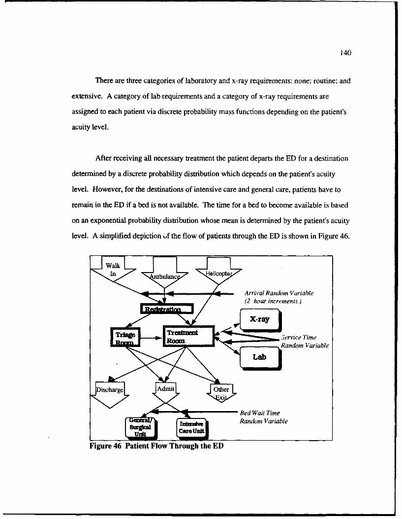
140
There are three categories of laboratory and x-ray requirements: none; routine; and
extensive. A category of lab requirements and a category of x-ray requirements are
assigned to each patient via discrete probability mass functions depending on the patient's
acuity level.
After receiving all necessary treatment the patient departs the ED for a destination
determined by a discrete probability distribution which depends on the patient's acuity
level. However, for the destinations of intensive care and general care, patients have to
remain in the ED if a bed is not available. The time for a bed to become available is based
on an exponential probability distribution whose mean is determined by the patient's acuity
level. A simplified depiction uf the flow of patients through the ED is shown in Figure 46.
Arrival Random Variable(2 hour increments.)
1w Service TimeRandom Variable
"•" Bed Wait Time
l Random Variable
Figure 46 Patient Flow Through the ED

141
7.2.3 Workers in the ED
The facilities and staff are divided into two categories, those that provide service
from a fixed station (e.g., treatment rooms and secretaries) and those that travel
throughout the ED (e.g., physicians and nurses). Based on these distinctions, the
stationary servers are modeled as resources and the mobile servers are modeled as
transporters in the SIMAN simulation. This allows the mobile servers to move freely
throughout the ED as well as to transport patients from one location to another. There
are three types of physicians: attending; third year residents; and first or second year
residents. There are six types of nurses: charge nurse; triage nurse; emergent patient area
nurse; urgent patient area nurse; non-urgent patient area nurse and nurses aide. Service
times of physicians and nurses and clerks are modeled as exponential distributions with
means dependent on the acuity level and care type of the patient. Service times of
registration and admittance personnel are modeled as uniform distributions with ranges
dependent on arrival mode and acuity level of the patient. Server breaks are combined
with lunches to give each worker the unofficial standard 45 minute lunch/dinner break
rather than the officially prescribed 30 minute lunch break and two ten minute breaks.
7.2.4 Validation of the Simulation
Using the CINEMA companion to SIMAN, an animation of the ED simulation
was developed and shown to hospital personnel to obtain face validation of the computer
simulation from the system operators. In addition, output data from the simulation was
compared with observed data from the ED system. The quantity of patients and time in
the system for different patient categories were extracted from the hospital databases for
two months, and estimates were made of mean values. These were compared to the
estimates from the simulation model, where the simulation results were the averages of ten

142
replications of 61, days or two months each. The comparisons are summarized in Table
21. These results show that the computer simulation accurately represents the actual ED.
Table 21 Simulation Com arison with Actual ED Database Records
Patient Number in Number in Database Average Simulation AverageType Database Simulation System Time (Min.) System Time (Min.)
Emergent 415 451 159 164Urgent 4091 4166 176 172Non Urgent 3963 3959 116 123Total 8469 8576 147 149
7.3 Demonstration of the Baseline ANN Metamodel Approach
In an environment such as the emergency department, where changes in the system
occur frequently and with little warning, tactical decisions need to be made quickly. The
simulation that was built to examine alternative solutions to problems in the emergency
department could not be run quickly enough to provide assistance to the ED management.
Thus a neural network metamodel of the ED simulation was constructed to demonstrate
the usefulness of the metamodel approach. The following discussion demonstrates the
application of the baseline ANN metamodel approach to the ED system.
7.3.1 Phase I of the Baseline ANN Metamodel Approach
The first phase of the baseline ANN metamodel approach requires close interaction
between the developer of the ANN metamodel and the operator of the system under
study. In this case the management of the ED wanted the simulation to be able to provide
a reliable estimate of the average time a patient spends in the ED, from arrival until
departure. Other simulation outputs of interest to ED personnel included, maximum time

143
patients spent in the ED, average time patients spent waiting for service, and utilization of
rates of the rooms and staff. The ED staff were also interested in the patient related
statistics being provided by each acuity type. To keep the demonstration simple, only the
most important output of average patient time in the ED was used.
Many different inputs to the simulation were described in Section 7.2. These
inputs range from arrival distributions, to percentages of patients of each acuity level, to
time to complete various services, to numbers of staff personnel on duty, to the time and
duration of staff breaks. The selection of which inputs should be included in the
metamodel is guided by the practical application of the metamodel. For this case, the ED
staff wanted to understand the effect of changing four specific input variables which were
outside of the direct control of the ED personnel but were within the control of other
sections of the hospital. The four input parameters of the emergency department
simulation examined in this research were the means of an exponential random variable for
intensive care bed wait time, general care bed wait time, laboratory service time, and x-ray
service time. As was described in Section 7.2, when patients leave the ED they might end
up waiting in the ED for a period of time for a bed within the hospital to become available;
i.e., either intensive care bed wait time or general care bed wait time.
For each of the input parameters, the initial values of these parameters in t'lj
simulation were obtained from a series of regression models of the hospital's actual patient
times in the emergency department. The initial values of these parameters were selected
as one of the training points for the neural networks. To obtain minimum and maximum
values for the variables, each of the parameters was permitted to take on values that were
+100% of the initial settings in the simulation. While additional values could have been

144
selected for developing the ANN metamodel of the computer simulation, the three values
per input parameter are enough to examine the relationship between the input variables
and the output measure. Since each of the four parameters had three possible values, the
total number of points in the training set was 81 data points. The plot of the training
points for each of the pairwise combinations of input parameters is shown in Figure 47.
The actual values of the input parameters and the response provided by ten replications uf
the simulation in terms of the mean and the variance of the mean time in the system is
provided in Table C1. The mean and the variance of the mean in Table Cl are determined
using equations 7-1 and 7-2. The number of replications was selected as ten since this
typically produced variances that were relatively small. The data was shuffled in the order
that was used to train the ANN.
In order to evaluate the generalization ability of the ANN, 80 test points were
selected from the region internal to the training set. The test points from a pairwise
comparison viewpoint are shown in Figure 48. The actual values of the input parameters
for the test set and the response provided by 100 replications of the simulation are shown
in Table C2. The mean and the variance of the mean in Table Cl are determined using
equations 7-3 and 7-4. It should be noted that equation 7-3 is actually calculating the
mean of ten averages of different sets of ten replications which is th, --',ve as calculating
the mean of the 100 replications. However, equation 7-4 is the mean of ten variances of
different sets of ten replications which is not the same as the variance of 100 replications.
The number of replications was chosen as 100 for the dissertation work however, in actual
application it would have been adequate to have ten replications for the test set. To
provide a comparison of how well direct simulation performs compared to the ANN
metamodels, an additional 20 replications were made and split into two groups of ten
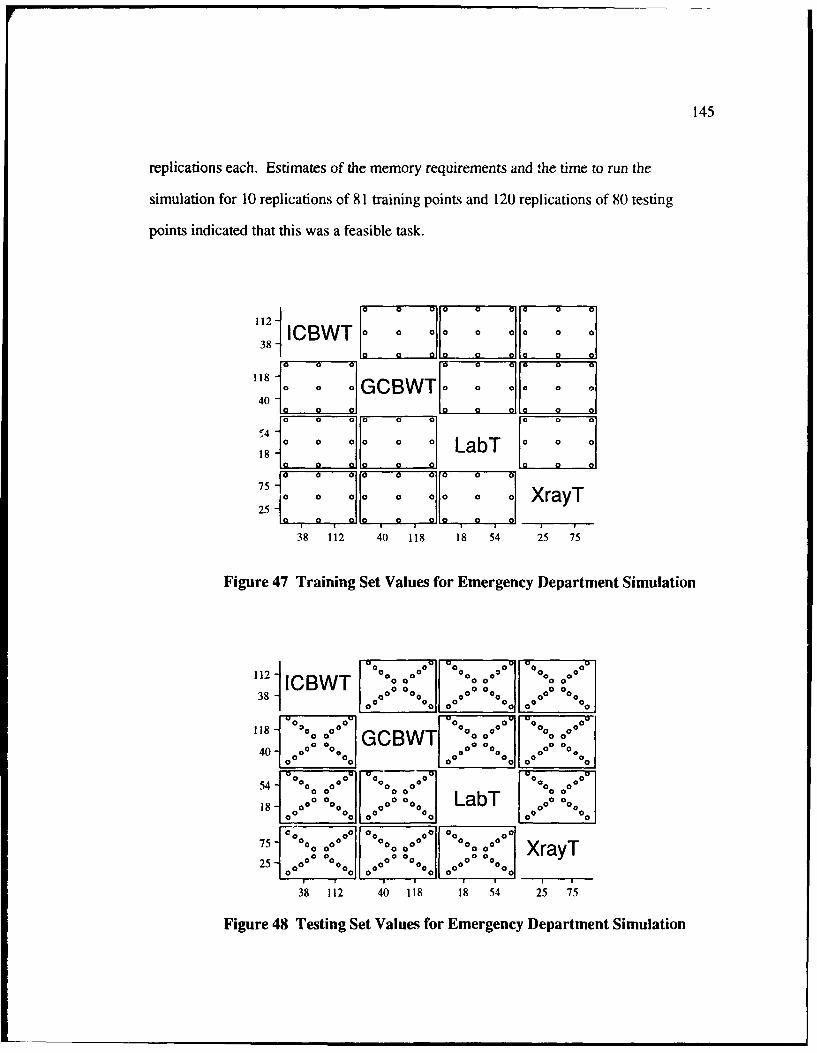
145
replications each. Estimates of the memory requirements and the time to run the
simulation for 10 replications of 81 training points and 120 replications of 80 testing
points indicated that this was a feasible task.
1121ICBWT
38s1
118f-lGCBWTK 7 ~40
r4 - LabT
751 ry
250 0 0 0 0 0
38 112 40 118 18 54 25 75
Figure 47 Training Set Values for Emergency Department Simulation
112 ICBWT 0
38000 00 00
118 OO 00 00
00
0
40 00 ° 0 00 00 000O000 0 00.
54-° o75 0 00000 0000 LabT 000 0 00
0o O0 O0O0
C0 lo. 0o 0 o o075 %0 *°o025 00o, 0000o*. oO 00000,ol°°° XrayT
2 -00 0 00 0 00 0L 4100 %00'
38 112 40 118 18 54 25 75
Figure 48 Testing Set Values for Emergency Department Simulation

146
10
S1=- (7-1)i 10
10
Var(Ti) = 9X1 (7-2)
10
T = j=1 (7-3)10
10
Vat(T) =i--1 (7-4)XlO10
7.3.2 Phase 2 of the Baseline ANN Metamodel Approach
In this phase, all three types of ANN that could be developed using the Baseline
ANN metamodel approach are demonstrated. The first two ANN estimate the average
time a patient spends in the emergency department: one using the individual replications
and one using the average values of the simulation. The third ANN estimates the variance
of the average time a patient spends in the emergency department.

147
The training data is shuffled to improve the learning process as ',hown in Table C l.
The minimum and maximum values for the output measures used to perform the scaling
for ANN training were selected to be +10% of the range beyond the minimum and
maximum values of the training and testing sets, respectively. The training tolerance was
set at 0.002 to ensure that the training would not ten , reaching the training
tolerance. The maximum number of epochs or runs through the training set was initially
set at 750. The initial BrainMaker files used for training for the individual replications,
averages, and variances are provided in Figures Cl, C3 and C5, respectively.
The architecture used for the ANN initially was four input nodes, two hidden
layers of two nodes each, and one output node. This network was trained using the "best
net training" technique and the best network for two nodes in each hidden layer was
evaluated on the test set. Another node was added to each hidden layer and the process
was repeated. The number of epochs to reach the best network was compared to the
maximum number of epochs permitted. For all three networks the best network was close
to the maximum number of epochs. Thus, the maximum number of epochs was increased
and training repeated with the maximum number of epochs being 1,000 for the ANN
predicting the mean time in the ED and 5,000 for the ANN predicting the variance of the
mean time in the ED. For these values of the maximum number of epochs, the networks
found their best nets at 870, 259, and 4,853 for the networks trained on individual
replications, averages and variances, respectively.
The results for the networks being used to predict mean time in the ED are shown
in Figure 49. As can be seen in Figure 49 four hidden nodes per layer results in the lowest
MAE on the test set. Ordinarily, the baseline ANN metamodeling approach would have

148
stopped the search for the best number of nodes in the hidden layers at five nodes since
that is where the networks begin to do worse on the test set. For demonstration purposes
the process was continued, for selected values out to 22 hidden nodes. As Figure 49
shows, in this case the procedure appears to have selected the best number of hidden
nodes. The same process was performed for the network predicting the variance of the
mean time in the ED with the result being that the selected number of hidden nodes was
seven. The final trained networks for the networks trained on individual replications,
averages, and variances are provided in Figures C2, C4 and C6, respectively.
I Averages (PM 1) 0 Replications (PM 4)
10.. Best Number of Nodes.9 9
7 --06
3
2
0 I I
0 5 10 15 20 25
Number of Nodes per Hidden Layer
Figure 49 Hidden Nodes for Predicting Mean Time in ED for the Test Set
7.3.3 Phase 3 of the Baseline ANN Metamodel Approach
The results of the ANN training and testing are examined in the third phase of the
baseline ANN metamodel approach in order to determine if additional training data is
required. The results of testing the ANN for the networks predicting the mean and the
networks predicting the variance of the mean are provided in Tables C3 and C4,

149
respectively. The summary results in terms of mean absolute error and maximum error
observed for the each of the ANN compared to the results of 100 replications of the
simulation are provide in Tables 22 and 23. Table 22 provides the results for all 80 test
points. Table 23 provides the results for 78 of the test points where the points with the
two worst errors have been removed. From Table 23 it can be seen that the mean
absolute errors of the networks predicting the mean time in the ED, of 2.13 and 1.81, are
very low in comparison to the average time in the ED which ranged in value from 115 to
180. The maximum errors of the same networks, 9.4 and 9.2 are also quite small. The
results are even more impressive when the two points with the worst testing errors are
removed as is shown in Table 23. The results for the variance predictions are not as
impressive. While the values for the variance of the test set ranged from 10 to 98, the
MAE was 8.6 and the maximum error was 95 as can be seen in Table 22. If the two worst
points are removed, the MAE drops to 6.7 and the maximum error drops to a more
respectable level of 33.1. This indicates that predicting the variance of the mean is much
more difficult than predicting the mean time in the ED.
Also shown in Tables 22 and 23 are the results of using two different sets of direct
simulation of the test set, each of size ten replications, to try to predict the "true" answers
obtained from direct simulation of 100 replications. Although this would not ordinarily be
done in the baseline ANN metamodel approach, the results are instructive. The ANN
outperform the ten replication direct simulation in every case except for the maximum
error of the variance when considering all 80 test points.

150
TABLE 22 Corn arisons To "True" ED Simulation (100 Replications)MAE Maximum Error
Estimation Data Used Mean Time Var (T) Mean Time Var (T)Method In ED (T) In ED (T)
Direct Simulation Set A - 10 Replications 4.33 14.16 13.03 69.90Direct Simulation Set B - 10 Replications 4.22 19.91 11.21 74.80Direct Simulation Average MAE of Sets A&B 4.28 17.03 12.12 72.35
ANN Averages (PM 1) 2.13 9.40ANN Individual Replications (PM 4) 1.81 9.20ANN Variance (T) 1 8.6 95.0
TABLE 23 Comparisons To "True" ED Simulation (100 Replications) When TwoWorst Errors Are Removed
MAE Maximum ErrorEstimation Data Used Mean Time Var (T) Mean Time Var (T)
Method In ED (T) In ED (T)Direct Simulation Set A - 10 Replications 4.02 12.42 11.70 61.2Direct Simulation Set B - 10 Replications 3.94 11.35 10.40 47.0Direct Simulation Average MAE of Sets A&B 3.98 11.88 11.05 54.1
ANN Averages (PM 1) 1.92 6.80ANN Individual Replications (PM 4) 1.60 4.80ANN Variance (T) i 6.7 33.1
In addition to examining the summary statistics, Figures 50 and 51 provide a visual
comparison of the ANN to the "true" answers of 100 replication of computer simulation at
the test points. Figures 50a through 50d compare the test set predictions for the network
trained on the individual replications for each of the input variables. Figures 50a through
50d all indicate that the ANN are able to closely approximate the mean time in the ED as
determined by the computer simulation. Figures 51a through 51d compare the test set
predictions for the network trained on the variances for each of the input variables.
Figures 51 a through 51 d indicate that while the variance is a more difficult function to
estimate, the ANN does a fairly good job of predicting the variance computer
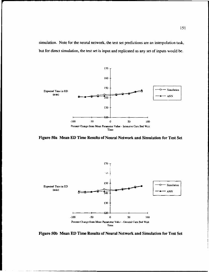
151
simulation. Note for the neural network, the test set predictions are an interpolation task,
but for direct simulation, the test set is input and replicated as any set of inputs would be.
170T
160
Expected Time in ED 15 Simulation
(min) ANN
130
-100 -50 0 50 100
Percent Change from Mean Parameter Value - Intensive Care Bed WaitTime
Figure 50a Mean ED Time Results of Neural Network and Simulation for Test Set
170 T
"50
Expected Time in ED 150 Simulation
(min) -A----ANN
130
-100 -50 0 50 100
Percent Change from Mean Parameter Valuý- - General Care Bed WaitTime
Figure 50b Mean ED Time Results of Neural Network and Simulation for Test Set
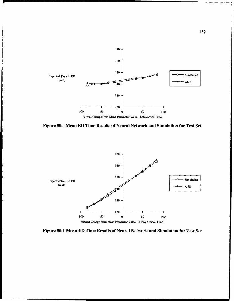
152
170
160
Expected Tune in ED 0 Simulation
(mim) -a--- ANN
130
-100 -50 0 50 100
Percent Change from Mean Parameter Value - Lab Service Time
Figure 50c Mean ED Time Results of Neural Network and Simulation for Test Set
170
160
150Expected Time in ED D Simulation
(min) 15 ANN
130
-100 -50 0 50 100
Percent Change from Mean Parameter Value - X-Ray Service Time
Figure SOd Mean ED Time Results of Neural Network and Simulation for Test Set
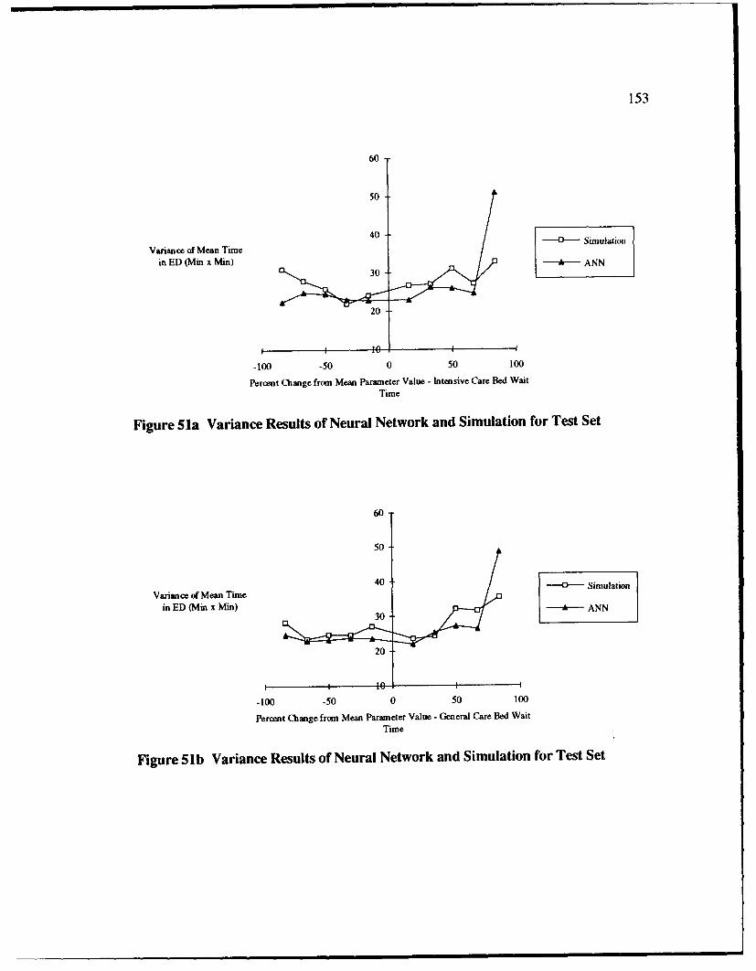
153
60
50
40 - Simulation
Variance of Mean Time
in ED (Min x Min) - ANN
20
-100 -50 0 50 100
Percent Change from Mean Parameter Value - Intensive Care Bed WaitTime
Figure 51a Variance Results of Neural Network and Simulation for Test Set
60
50
Variance of Mean Time 40 Simulation
in ED (Min x Min) -i-30 ANN
20
-100 -50 0 50 100
Percent Change from Mean Parameter Value - General Care Bed WaitTime
Figure 51b Variance Results of Neural Network and Simulation for Test Set
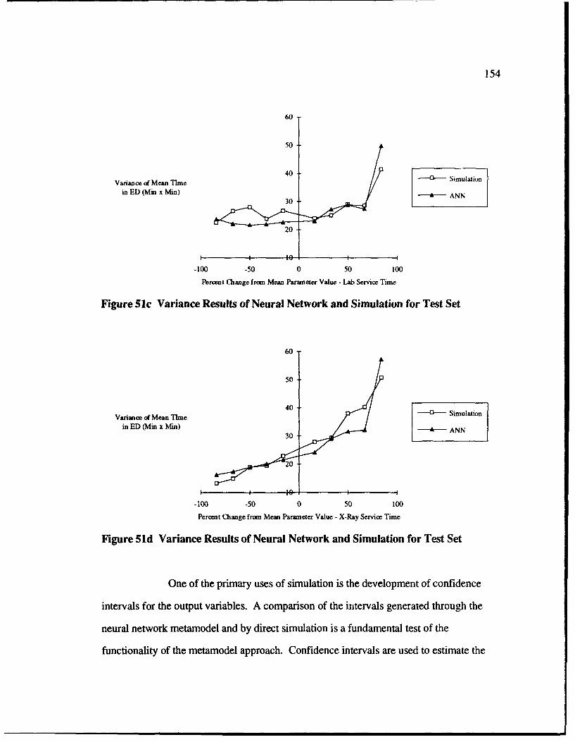
154
60
Variance of Mean Time 40 Simulation
in ED (Min x Min) • ANN30
-100 -50 0 50 100
Percent Change from Mean Parameter Value - Lab Service Time
Figure 51c Variance Results of Neural Network and Simulation for Test Set
60
50
40- - SimulationVariance of Mean Time
in ED (Min x Min) • ANN30
-100 -50 0 50 100
Percent Change from Mean Parameter Value - X-Ray Service Time
Figure Sid Variance Results of Neural Network and Simulation for Test Set
One of the primary uses of simulation is the development of confidence
intervals for the output variables. A comparison of the intervals generated through the
neural network metamodel and by direct simulation is a fundamental test of the
functionality of the metamodel approach. Confidence intervals are used to estimate the

155
range within which one expects the mean to fall. In regression, prediction intervals are
used to estimate the range within which an individual observation would be expected to
fall. In the simulation and statistics fields tolerance intervals are used rather than
prediction intervals since the mean and variance are unknown. In regression the mean and
variance are assumed to be known when in fact they are not truly known.
Since ANN are also metamodels of the computer simulation, it is appropriate to
use prediction intervals for ANN. For comparison purposes prediction intervals are also
constructed in this research for the computer simulation output. Prediction intervals for
confidence factors of 80%, 90%, 95% and 99% were generated for the test set using the
first set of ten extra replications of the simulation and the two parallel neural metamodels
(one for expected time and the other for variance). Table 24 shows the comparison of
these intervals by the number of 100 separate simulation replications which fell within the
interval, fell on the low side of the interval and fell on the high side of the interval. Table
24 shows that the neural network was very accurate in terms of the appropriate number of
replications falling within the intervals, and the neural network trained on individual
replications was slightly more precise than that trained on means. In fact, for the 80% and
90% intervals the ANN did too well, in that the number falling in the interval was larger
than expected. For the 95% and 99% intervals the ANN were closer to the desired levels
than the intervals developed using direct simulation data. What this implies is the ANN
are too accurate at the 80% and 90% level, to be characterized as being generated by ten
replications and that a more appropriate number of replications to enter the t-table for the
ANN would be some number larger than ten.
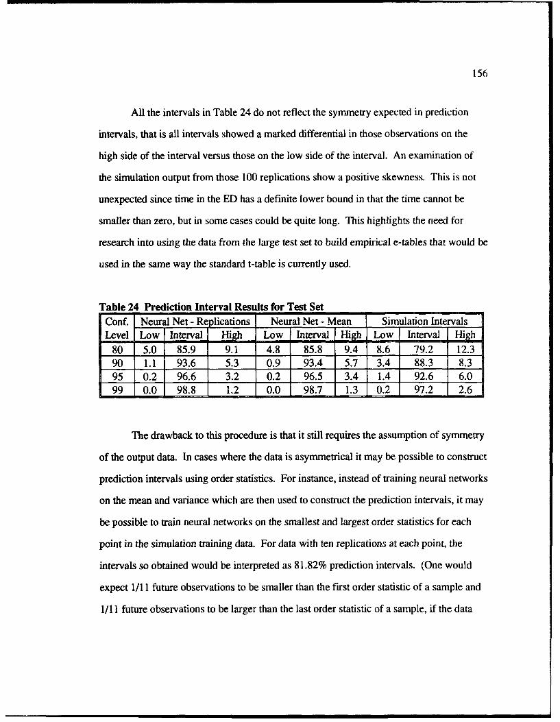
156
All the intervals in Table 24 do not reflect the symmetry expected in prediction
intervals, that is all intervals showed a marked differential in those observations on the
high side of the interval versus those on the low side of the interval. An examination of
the simulation output from those 100 replications show a positive skewness. This is not
unexpected since time in the ED has a definite lower bound in that the time cannot be
smaller than zero, but in some cases could be quite long. This highlights the need for
research into using the data from the large test set to build empirical e-tables that would be
used in the same way the standard t-table is currently used.
Table 24 Prediction Interval Results for Test Set
Conf. Neural Net - Replications Neural Net - Mean Simulation IntervalsLevel Low Intervall High Low Interval High Low Interval High
80 5.0 85.9 9.1 4.8 85.8 9.4 8.6 79.2 12.390 1.1 93.6 5.3 0.9 93.4 5.7 3.4 88.3 8.3
95 0.2 96.6 3.2 0.2 96.5 3.4 1.4 92.6 6.099 0.0 98.8 1.2 0.0 98.7 1.3 0.2 97.2 2.6
The drawback to this procedure is that it still requires the assumption of symmetry
of the output data. In cases where the data is asymmetrical it may be possible to construct
prediction intervals using order statistics. For instance, instead of training neural networks
on the mean and variance which are then used to construct the prediction intervals, it may
be possible to train neural networks on the smallest and largest order statistics for each
point in the simulation training data. For data with ten replications at each point, the
intervals so obtained would be interpreted as 81.82% prediction intervals. (One would
expect 1/11 future observations to be smaller than the first order statistic of a sample and
1/11 future observations to be larger than the last order statistic of a sample, if the data

157
comes from a continuous distribution. This leaves 9/11 future observations to fall
between the first and last order statistics.)
On the basis of these results of the summary statistics of MAE and maximum
error, the graphical comparison over the range of test set values for each of the input
parameters, and the prediction intervals it appears that there is no requirement to obtain
additional training data.
7.4 Results of ED System Demonstration
As can be seen from Table 22, the ANN using individual replications performs
better than the ANN trained on averages which collaborates the observations from the
experiments performed on the inventory simulation. In addition, the ANN metamodels
produced better results when trying to predict the "true" mean time in the system and the
variance of the mean time in the system than direct simulation of 10 replications. The
conclusion to be drawn from these results is that rather than perform direct simulation for
various additional combinations of the simulation input parameters, the ANN metamodels
could be used to give more accurate estimates of the average patient time in the system
without making any additional runs of the computer simulation.
As Figures 50 and 51 indicate, the neural network did extremely well on
generalizing its training to the test set. The expected value of time in the system was an
easier problem to learn, and therefore predictions are more accurate than for the variance.
Variance predictions could probably be improved by training the variance neural network
metamodel on sets of replications, i.e., use ten sets, of ten replications each, to develop ten

158
different variance values for each input vector. This of course would also ilciease the
amount of work to develop the neural network metamodel since 100 replications, instead
of ten replications, would be required at each training and testing point.
7.5 Summary
This chapter contains the results of applying the baseline ANN metamodel
approach to a demonstration problem. The demonstration problem is based on a
computer simulation of an emergency department. The computer simulation is described
in terms of the physical layout, flow of patients, and workers in the emergency
department. The computer simulation is shown to be a valid representation of the
emergency department. The input parameters of concern were the intensive care bed wait
time, general care bed wait time, laboratory service time, and X-ray service time. The
output measure of interest was the time that patients spent in the emergency department.
A total of 81 training points and 80 testing points were selected. The baseline ANN
metamodel procedure was followed in developing ANN metamodels of the mean time in
the ED using both individual replications and average values. An additional ANN
metamodel was constructed to predict the variance of the mean time in the ED. The
results of following the baseline ANN training procedure were that the ANN predicting
mean time in the ED used four hidden nodes in each of two hidden layers and the ANN
predicting the variance of the mean time in the ED used seven hidden nodes in each of two
hidden layers. The ANN metamodels as well as two different sets of ten replications of
direct simulation of the test set were compared to the "true" response of 100 replications
of direct simulation. The results indicated that the ANN metamodels were better
predictors than ten replications of direct simulation for both the mean time in the ED and

159
the variance of the mean time in the ED as shown in Tables 22 and 23.. This should not
be taken as a suggestion that the ANN metamodels are performing better than the
computer simulation. The only conclusion that should be inferred from these results is
that the ANN metamodel appears to be more accurate on the test set than ten replications
of the computer simulation. Additionally, the metamodels of the mean time in the ED and
the variance of the mean time in the ED were combined to develop prediction intervals.
The ANN and direct simulation prediction intervals were both skewed in that more of the
100 observations at each testing point fell to the right than fell to the left of the prediction
interval. This observation is not unexpected since time in system data does tend to be
skewed to the right since there is a definite lower bound of zero. This observation
highlights the need for researching non-paraimetric methods of constructing confidence
and predictions intervals for metamodels. This chapter has demonstrated the application
of the baseline ANN metamodel approach and shows how the approach can be beneficial
to the simulation of real world systems.

160
8.0 SUMMARY AND CONCLUSIONS
The baseline ANN metamodel approach to approximating discrete event computer
simulations has been demonstrated in this research to be a viable and effective way to
develop accurate metamodels of computer simulations.
8.1 The Baseline ANN Metamodel Approach
The experiments discussed in Chapters 4 and 5 on the inventory computer
simulation were used to develop and refine the baseline ANN metamodel approach. The
specific steps entailed in the approach are provided in detail in Chapter 6. The baseline
approach involves using a backpropagation trained artificial neural network to learn the
relationship between the simulation inputs and output. The approach consists of three
phases. The first phase is to determine what simulation information is of interest in terms
of the inputs and outputs of the simulation, to estimate the time required to obtain the
simulation information and to obtain the information by running the computer simulation.
Training and testing data are obtained from the first phase. The second phase is to
develop a neural network approximation of the computer simulation using the data
obtained from the first phase as training examples to be learned by a backpropagation
trained, full connected, feedforward artificial neural network. The specific form of
training that is used is called "best net training." The third phase is to evaluate the results
of the trained ANN to determine if additional simulation data is required. The baseline
ANN metamodel approach was applied to a large emergency department simulation and
the results are provided in Chapter 7 to demonstrate the application of the approach on a
real world problem.

161
8.2 The Performance of the Baseline ANN Metamodel Approach
The results of the (s,S) inventory development problem showed that in terms of
accuracy ANN metamodels outperform regression metamodels of the type typically used
in response surface methods. The results of this research also show that it is better to use
separate networks for different outputs than to have a combined network. In addition, it
was shown that networks trained on the individual replication output data had better
generalization performance than networks trained on just the averages of the simulation
output. As was shown in Chapter 7, the baseline ANN metamodel approach can do well
at approximating a computer simulation. In fact, for the demonstration problem, the ANN
metamodel trained on 81 data points each with ten replications was able to outperform
direct simulation of ten replications on 80 additional test points which were not included in
the training set.
It must be noted that neural networks and the other metamodeling techniques
commonly used are deterministic. The stochastic aspect of the simulation is lost, however,
the metamodel is much faster in operation than the simulation. Therefore, while possibly
losing precision when moving from the simulation to a metamodel, the user also loses the
rich stochastic framework of the simulation. Surrogates for the stochastic elements, such
as expected value, moments and percentiles, must be used in deterministic metamodels.
Thus the tradeoffs involve imprecision and simplification for increased speed.
One disadvantage of the ANN metamodel is that it is even more of a "black box"
than the original computer simulation. While sensitivity analysis can be performed using
the ANN metamodel, it does not have the advantage of the convenient interpretation of
the coefficients found in regression metamodels.

162
8.3 Major Contributions of the Dissertation
The major contribution of this dissertation is the development of a baseline
approach for developing ANN metamodels of computer simulations. This baseline
approach can be used by other researchers for comparison purposes when developing their
own ANN metamodel approaches. This contribution was needed in the field of artificial
neural networks because there are many different existing and emerging ANN procedures
for performing approximation and estimation tasks. Another specific contribution is the
determination that it is best when approximating stochastic computer simulations to use
the "noisy" individual replications rather than the "quiet" average values. While the results
of this research indicate that ANN are appropriate for use as metamodels of stochastic
computer simulations, this research has identified many areas that require additional work
and experimentation to take proper advantage of ANN as metamodels.
8.4 Future Research Directions
There are many new research issues that have arisen as a result of the experiments
and work performed for this dissertation. The major areas of future research work are
divided into three categories: improvements on the baseline ANN metamodel approach,
extensions of the approach, and specific applications or uses of the approach.
8.4.1 Improvements of the Baseline ANN Metamodel Approach
A major area of research is in experimental design for neural networks as
metamodels of computer simulations. The need for research into experimental design

163
considerations exists for all types of metamodels.( 142) The most critical need is for designs
that take into consideration both the development (i.e., training) and the evaluation (i.e.,
testing and validation) of metamodels. This becomes even more critical if the metamodels
are to be constructed using a training set for adjusting the weights and one test set for
determining when to stop training and a second test set for evaluation of the generalization
ability of the metamodel. Work should build on the research performed using traditional
designs from statistics and response surface methods and also those proposed by Taguchi.
A new procedure that could improve the performance of the ANN metamodel
approach is ensemble networks.(1 43) The basic idea is to build several different networks
and take the average of their output in order to build a more robust overall network
metamodel. This procedure was examined briefly in this research, but is not reported in
this document due to it being outside the scope of this research. One idea that was
considered in the work supporting this research was to combine the outputs of the
networks trained on the different subsets of the training set discussed in Chapters 4 and 5.
Other approaches could be to train different networks on different training parameters, on
different initial weights, or on different orderings of the training data.
Another area of potential research where success has been achieved with
regression metamodels used in RSM is the use of common random numbers and other
variance reduction techniques. In this research, all of the simulation data was generated as
independent observations for both the training and testing data.
Other research is needed to examine various iterative approaches for developing
improvements beyond the baseline ANN metamodeling approach. For instance, it might

164
make more efficient use of the computer simulation to start with small training and testing
sets, in terms of replications, and build ANN metamodels to use in performing factor
screening to eliminate those input factors that do not appear to make much of a difference
on the simulation output. After eliminating the irrelevant factors the baseline approach
could be used on the remaining factors with a substantial savings in total computer
simulation runs. Another issue that could be addressed using iterative methods, is to
determine what steps should be taken, if any, after developing an ANN and evaluating it
on the test set, to improve the ANN. Possible steps would include determining the regions
of the input space where the ANN is performing poorly and then deciding on the
appropriate corrective action such as obtaining more data points for training or more
replications for data points already in the training set.
Research is also needed on the use of extreme values observed from the
simulation. For instance in the hospital simulation one of the average output values for a
particular combination of the input training parameters, was much larger than all of the
other average output values. The research issue would be to determine if such values
should be included in the training set.
Another research issue that needs to be examined is a comparison between the
confidence intervals obtained using metamodels of the mean and variance versus the
confidence intervals obtained using metamodels derived from the lower and upper
confidence limits of each point in the input parameter training space as was done in
Hurrion's work.(76)

165
Finally, another major area for future research is examining faster training
procedures and alternative types of neural networks that have been developed since the
introduction of backpropagation. Networks such as RPROP and radial basis function
(RBF) networks are two such candidates.
8.4.2 Extensions of the Baseline ANN Metamodel Approach
One area of research interest is to extend the application of the baseline ANN
metamodel approach to predictions over time as opposed to terminal values or values
averaged over the length of the simulation run.
A second extension of the ANN approximation approach is to model non-
terminating simulations. Some of the new approaches such as infinitesimal perturbation
analysis which use one long single run of the simulation rather than many replications may
be a useful way to obtain data for training a neural network metamodel of a simulation.
A third area for future extensions of the baseline ANN metamodel is to develop
empirical confidence and prediction intervals rather than intervals based on the Normal or
t-tables.
One of the drawbacks of the approach developed in this research is that it
transforms a stochastic computer simulation into a deterministic ANN metamodel. In
some applications, such as modules within a very large computer simulation, the stochastic
nature of the module is esser ,ial to the proper operation of the computer simulation.
Thus, another area of research is to build a family of ANN that would attempt to capture
more than just the mean and variance of the output of the simulation. This family of ANN

166
would have n members, one for each of the n replications, and each member would be
trained on just one of the order statistics for all points in the input training space. In this
way the entire cumulative distribution function for each point in the input parameter space
could be estimated. Using this estimated cumulative distribution function and the inverse
transform method it would be possible to replace a large module in a computer simulation
with a stochastic rather than a deterministic approximation. This is an important
consideration since models are being used to do more than analysis. Simulation models
are being used for training in industry and to support large scale exercises in the military.
Future generations of such simulations which will incorporate advanced features such as
virtual reality will also need ways of aggregating models that are appropriately
stochastic.(144)
8.4.3 Applications of the Baseline ANN Metamodel Approach
One application of ANN metamodels that needs additional research is in response
surface methods. Based on the work in this research ANN trained for a very short time,
say only a few epochs, may very well provide an adequate estimate to perform response
surface optimization. Response surface methods estimate the shape of the response
surface in a small region and move away from that region toward improvement in the
measure of interest. Additional data is then gathered to estimate the surface in the new
region and the process is repeated until there is evidence that an optimum has been
reached. Based on the results of this research which found the errors of the training and
testing sets decreasing rapidly after one or two epochs it may be possible for ANN to
replace first-order regressions in finding the direction of improvement in response surface
methods. However, first-order regressions have the advantage of knowing the direction
of improvement by just calculating the derivative of the first-order regression equation. A

167
more suitable use of ANN in traditional RSM would probably be as a replacement to the
second-order regressions which are used to determine if the RSM procedure has reached
the optimum and should terminate. In this portion of the RSM procedure, accuracy is
more important than speed. The results of this research have shown ANN metamodels
can be more accurate than second- order regression metamodels and therefore have the
potential for improving the termination portion of response surface methods. Additional
research is needed that compares ANN and regression metamodels in traditional response
surface methods.
Another area of research is the application of using neural networks trained on
computer simulations to "feed" non-gradient based optimization procedures such as
genetic algorithms and simulated annealing. In these approaches, the only thing needed by
the optimization procedure is an objective function or "fitness function" that informs the
optimization procedure of the value of the output measure or the "fitness" of a particular
combination of the input parameters.(145) In these types of optimization procedures, the
added information of the direction of improvement in first-order regression models is of
no benefit. The fitness function could be the direct simulation, however, that could cause
the optimization procedure to be very slow.
An alteinative is to use a metamodel of the simulation as the fitness function. The
metamodel would need to be more global in nature than the metamodels used in traditional
response surface methods. In traditional RSM, the search begins at one random point and
slowly moves along successive approximations of the response surface towards the
optimum. In a genetic algorithm based procedure, the search would begin at many
different points and find promising areas that would warrant additional investigation.

168
After finding the most promising areas, it might be necessary to obtain additional
simulation runs to develop more accurate metamodels in the most promising areas. Thus,
the genetic algorithm approach would proceed from crude metamodels of a very large
region to increasingly accurate metamodels in smaller regions of the response surface.
Research into non-gradient based optimization procedures using ANN metamodels to
optimize computer simulation is needed to determine if such approaches would be
competitive with the traditional response surface methods.
In situations where limited system data is available, research efforts are needed to
explore ways of using that information in concert with computer simulation to improve the
validity of ANN metamodels. One simple approach is to adjust the results of the
computer simulation based on ANN trained on real system data. Suppose a small set of
input and output data, set A, is available for both the real sý stem and the computer
simulation. Train two different ANN: one on set Ar, from the real system and one on set
Ac, from the computer simulation. Additional data is obtained from the computer
simulation on a much larger data set B with each input point x having an average output of
y(x). Since the computer simulation may be a biased model of the true system, the
computer simulation results from data set B are adjusted using the neural networks
developed on the smaller data set A on the real system data and on the simulation data.
One adjustment of the output value of y(x) for each input point x of data set B that could
be made is shown in equation 8-1. The simulation data adjusted to be closer to the real
system data would then be used to train a third neural network. Such an approach could
be used to keep large computer simulations from being rebuilt every time there is a change
in the system. In addition, this type of approach could also be used as a procedure for
validating new computer simulations of existing systems.

169
Adjusted y = y x ANN Trained on Real System Data (x) (8-)ANN Trained on Computer Simulation Data (x)
One final application of metamodels created with the baseline ANN metamodel
approach that requires additional research is as on-line process controllers. In this
capacity the ANN are trained off-line using computer simulations and then are used on-
line to assist in the control of the process. In addition, the ANN metamodels could
continue to be improved and adjusted off-line as additional real system data and computer
simulation data becomes available. The conceptual approach presented by Wan and
Cochran should be applied and examined.(92)
8.5 SUMMARY
The ANN approach to approximating discrete event computer simulations has
been shown to be an effective way of developing accurate metamodels of computer
simulations. The results of experiments on a development problem of a simple simulation
led to the baseline ANN metamodel approach. The approach was used on a computer
simulation of a real system to clearly demonstrate the approach and its resulting benefits to
the simulation community. This chapter summarizes the baseline ANN metamodel
approach, the results of applying the approach, the contributions of the dissertation and
the specific suggestions for additional research in improving the baseline ANN metamodel
approach, for extending the approach to handle different types of problems, and for areas
in which the approach has application potential.

APPENDIX A
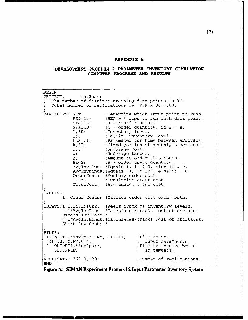
171
APPENDIX A
DEVELOPMENT PROBLEM 2 PARAMETER INVENTORY SIMULATIONCOMPUTER PROGRAMS AND RESULTS
BEGIN;PROJECT, inv2par;; The number of distinct training data points is 36.; Total number of replications is REP x 36= 360.
VARIABLES: GET: !Determine which input point to read.REP, 10: !REP = # reps to run each data point.SmallS: !s = reorder point.SmallD: !d = order quantity, if I = s.1,60: !Inventory level.Io: !Initial inventory level.tba,.l: !Parameter for time between arrivals.k,32: !Fixed portion of monthly order cost.u,5: !Underage cost.w: !Underage factor.Z: !Amount to order this month.BigS: 1S = order up-to quantity.AvgInvPlus: !Equals I, if I>0, else it = 0.AvgInvMinus:!Equals -I, if I<0, else it = 0.OrderCost: !Monthly order cost.COST: !Cumulative order cost.TotalCost; !Avg annual total cost.
TALLIES:1, Order Costs; !Tallies order cost each month.
DSTATS:I,I,INVENTORY: !Keeps track of inventory levels.2,1*AvglnvPlus, !Calculates/tracks cost of overage.Excess Inv Cost:!3,u*AvgInvMinus,!Calculates/tracks ('("st of shortages.Short Inv Cost;
FILES:l,INPUTl,"inv2par.IN", DIR(17) !File to set"(F3.0,lX,F3.0)": ! input parameters.2, OUTPUTl,"inv2par", !File to receive Write
SEQFREE; I statements.
REPLICATE, 360,0,120; !Number of replications.END;
Figure Al SIMAN Experiment Frame of 2 Input Parameter Inventory System
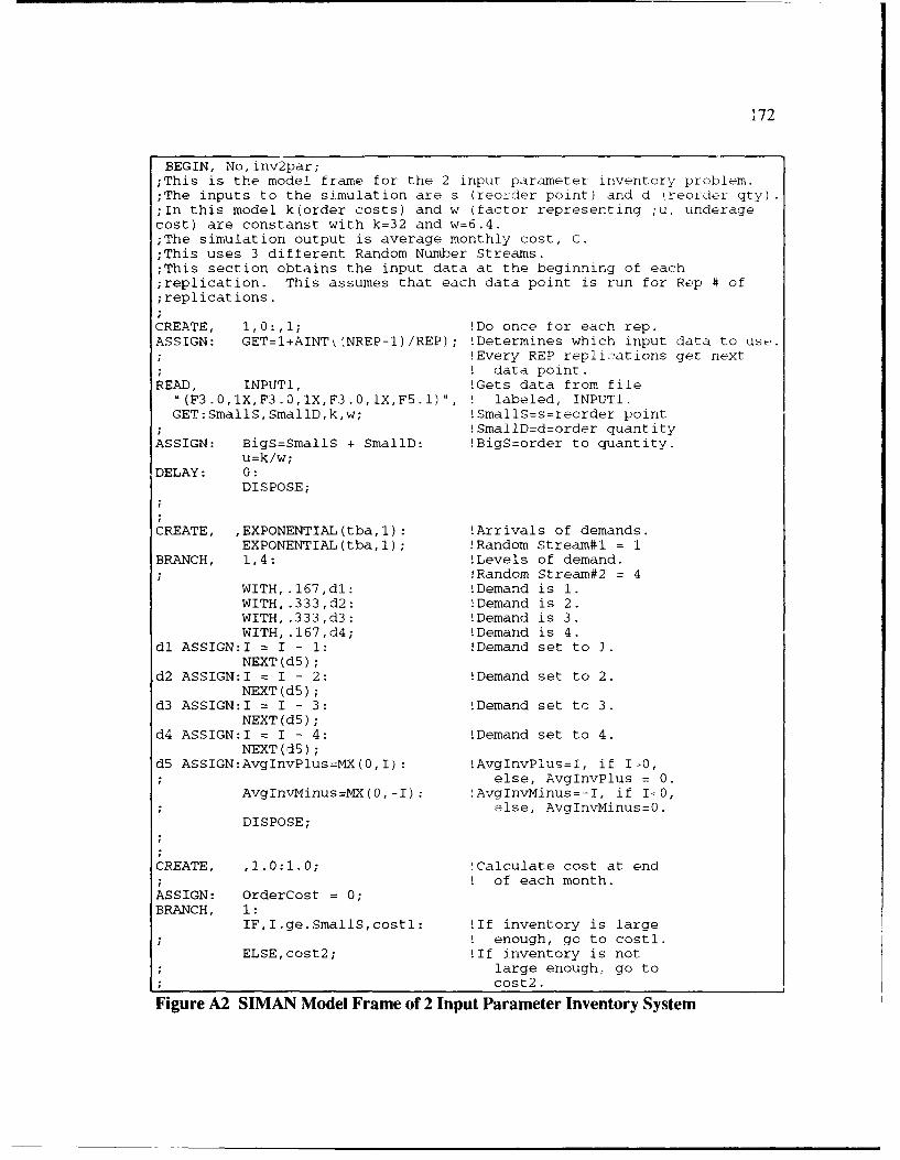
172
BEGIN, No, inv2par;;This is the model frame for the 2 input parameter inventory problem.;The inputs to the simulation are s (reorder point) and d (reorder qty).;In this model k(order costs) and w (factor representing ;u, underagecost) are constanst with k=32 and w=6.4.;The simulation output is average monthly cost, C.;This uses 3 different Random Number Streams.;This section obtains the input data at the beginning of each;replication. This assumes that each data point is run for Rep # of;replications.
CREATE, 1,0:,l; !Do once for each rep.ASSIGN: GET=I+AINTkNREP-I)/REP); !Determines which input data to use.
!Every REP replications get next! data point.
READ, INPUTI, !Gets data from file"(F3.0,lX,F3.0,lX,F3.0,lX,F5.I)", ! labeled, INPUT1.GET:SmallS,SmallD,k,w; !SmallS=s=reorder point
!SmallD=d=order quantityASSIGN: BigS=SmallS + SmallD: !BigS=order to quantity.
u=k/w;DELAY: 0:
DISPOSE;
CREATE, ,EXPONENTIAL(tba,l): !Arrivals of demands.EXPONENTIAL(tba,l); !Random Stream#1 = 1
BRANCH, 1,4: !Levels of demand.!Random Stream#2 = 4
WITH,.167,dl: !Demand is 1.WITH,.333,d2: !Demand is 2.WITH,.333,d3: !Demand is 3.WITH,.167,d4; !Demand is 4.
dl ASSIGN:I = I - 1: !Demand set to 1.NEXT(d5);
d2 ASSIGN:I = I - 2: !Demand set to 2.NEXT(d5);
d3 ASSIGN:I = I - 3: !Demand set to 3.NEXT(d5);
d4 ASSIGN:I = I - 4: !Demand set to 4.NEXT(dS);
d5 ASSIGN:AvgInvPlus=MX(0,I): !AvgInvPius=f, if 10,else, AvgInvPlus = 0.
AvgInvMinus=MX(0,-I): !AvgInvMinus=-I, if 1<0,else, AvgInvMinus=0.
DISPOSE;
CREATE, ,1.0:i.0; !Calculate cost at end! of each month.
ASSIGN: OrderCost = 0;BRANCH, 1:
IF,I.ge.SmallS,costl: !If inventory is large! enough, go to costl.
ELSE,cost2; !If inventory is notlarge enough, go tocost2.
Figure A2 SIMAN Model Frame of 2 Input Parameter Inventory System

173
costl ASSIGN:Z = 0; !Nothing ordered this month.TALLY: 1, OrderCost:DISPOSE;
cost2 ASSIGN:Z = (BigS-I); !Order Z amount.ASSIGN:OrderCost= k+3*Z; !Cost spent on orders this month.ASSIGN:COST = !Cumulative cost
COST + OrderCost; ! of orders to date.TALLY: 1, OrderCost;DELAY: UNIFORM(.5,1.0,8); !Wait for order arrival.
!Random Stream#3 = 8
ASSIGN: I = I + Z: !Increase inventory by ZAvgInvPlus=MX(0,I) : !AvgInvPlus=I, if I>0,
, else AvgInvPlus = 0.AvgInvMinus=MX(0,-I): !AvgInvMinus=-I, if I<0,
else AvgInvMinus = 0.DISPOSE;
CREATE, ,120:1,1; !After 10 year period,ASSIGN: TotalCost= . calculate average
TAVG(1)+DAVG(2)+DAVG(3); ! monthly total cost asthe sum of average;order,overage &underage costs.
WRITE, OUTPUT1,"(IX,2(F5.l,lX),Fl0.5)":SmallS, SmallD, TotalCost:DISPOSE;
END;
Figure A2(Continued) SIMAN Model Frame of 2 Input Parameter InventorySystem
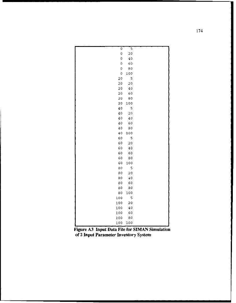
174
0 5
0 20
0 40
0 600 80
0 100
20 5
20 20
20 40
20 60
20 80
20 100
40 5
40 20
40 40
40 60
40 80
40 10060 5
60 20
60 40
60 60
60 80
60 10080 5
80 20
80 40
80 60
80 80
80 100
100 5
100 20
100 40
100 60
100 80
100 100
Figure A3 Input Data File for SIMAN Simulationof 2 Input Parameter Inventory System
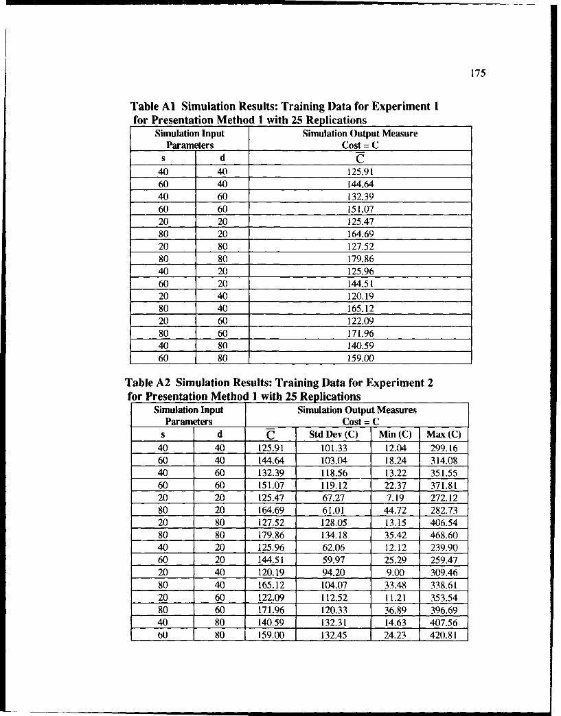
175
Table Al Simulation Results: Training Data for Experiment Ifor Presentation Method I with 25 Replications
Simulation Input Simulation Output MeasureParameters Cost = C
s d c40 40 125.9160 40 144.6440 60 132.3960 60 151.0720 20 125.4780 20 164.6920 80 127.5280 80 179.8640 20 125.9660 20 144.5120 40 120.1980 40 165.1220 60 122.0980 60 171.9640 80 140.5960 80 159.00
Table A2 Simulation Results: Training Data for Experiment 2for Presentation Method 1 with 25 Replications
Simulation Input Simulation Output MeasuresParameters Cost = C
s d Std Dev (C) Min (C) Max (C)
40 40 125.91 101.33 12.04 299.1660 40 144.64 103.04 18.24 314.0840 60 132.39 118.56 13.22 351.5560 60 151.07 119.12 22.37 371.8120 20 125.47 67.27 7.19 272.1280 20 164.69 61.01 44.72 282.7320 80 127.52 128.05 13.15 406.5480 80 179.86 134.18 35.42 468.6040 20 125.96 62.06 12.12 239.9060 20 144.51 59.97 25.29 259.4720 40 120.19 94.20 9.00 309.4680 40 165.12 104.07 33.48 338.6120 60 122.09 112.52 11.21 353.5480 60 171.96 120.33 36.89 396.6940 80 140.59 132.31 14.63 407.56
1 _00 80 159.00 132.45 24.23 420.81

176
Tab Simulation Results: ANN Testing Data for Experiment ISimulation Input Parameters Simulation Output Measure
s d ?C10 10 167.0250 10 135.3290 10 174.9810 50 125.6490 50 178.1110 90 130.9650 90 154.0190 90 194.2930 30 119.5250 30 132.9270 30 152.4230 50 122.1650 50 138.2570 50 157.9630 70 128.4i50 70 145.3670 70 165.47
Table A4 Simulation Results: ANN Testing Data for Experiment 2Simulation Input Parameters Simulation Ouptut Measures
s d C Std Dev(C) MNin(C) Max(C)
10 10 167.02 58.95 14.21 337.3550 10 135.32 28.57 31.14 210.6590 10 174.98 29.23 70.91 270.6810 50 125.64 100.64 13.29 352.6390 50 178.11 112.88 41.14 394.5010 90 130.86 135.18 16.62 461.3050 90 154.01 138.99 19.48 445.7290 90 194.29 140.77 46.63 510.7030 30 119.52 86.15 9.38 271.2150 30 132.92 88.40 14.00 276.3470 30 152.42 88.96 27.81 299.0030 50 122.16 107.79 11.04 318.1250 50 138.25 111.45 15.58 330.3970 50 157.96 112.04 27.96 353.8430 70 128.45 123.46 12.21 374.6150 70 145.36 125.74 17.58 387.8970 70 165.47 126.74 30.87 411.06

177
input number 1 2output number 1 1hidden 2 2
filename testfacts nn.tstfilename trainfacts j I a 113.fctfilename teststats j I a 113.sta
learnrate 1.0000 50 1.0000 75 1.0000 90 1.0000learnlayer 1.0000 1.0000 1.0000traintol 0.100 0.1000 0.8000 100testtol 0. 1000maxruns 5000smoothing 0.9000 0.9000 0.9000addhidden sequence 0.1 200
function hidden l sigmoid 0.0000 1.0000 0.0000 1function hidden2 sigmoid 0.0000 1.0000 0.0000 1function output sigmoid 0.0000 1.0000 0.0000 1
dictionary input s ddictionary output tcdisplay network progress
scale input minimum05scale input maximum100 100scale output minimum50scale output maximum225statistics 0 0 0weights 4 1 2 2 2 1-1.5510 0.6200 3.06203.1592 -4.5006 -0.32100.3232 5.6954 -6.7302-1.4922 -1.0282 2.9280
0.1166 2.5932 0.2082Figure A4 Initial Brainmaker Training File for Experiment I forPresentation Method 1 with 25 Replications

I178
input number 12output number I Ihidden 2 2
filename testfacts nn.tstfilename trainfacts j I a I 13.fctfilename teststats j I a 113. sta
learnrate 1.0000 50 1.0000 75 1.0000 90 1.0000learnlayer 1.0000 1.0000 1.0000traintol 0.1000 0.1000 0.8000 100testtol 0. 1000maxruns 2688smoothing 0.9000 0.9000 0.9000addhidden sequence 0.1 200
function hidden i sigmoid 0.0000 1.0000 0.0000 1function hidden2 sigmoid 0.0000 1.0000 0.0000 1function output sigmoid 0.0000 1.0000 0.0000 1
dictionary input s ddictionary output tcdisplay network progress
scale input minimum05scale input maximum100 100scale output minimum50scale output maximum225statistics 2688 863 167weights 4 1 2 2 2 1-2.7802 -0.0096 2.05402.4082 -4.9984 -1.2006
0.3232 5.6954 -6.7302-2.9304 -0.5290 2.0776
0.7850 2.3508 -0.9942Figure A5 Trained Brainmaker File for Experiment I forPresentation Method 1 with 25 Replications
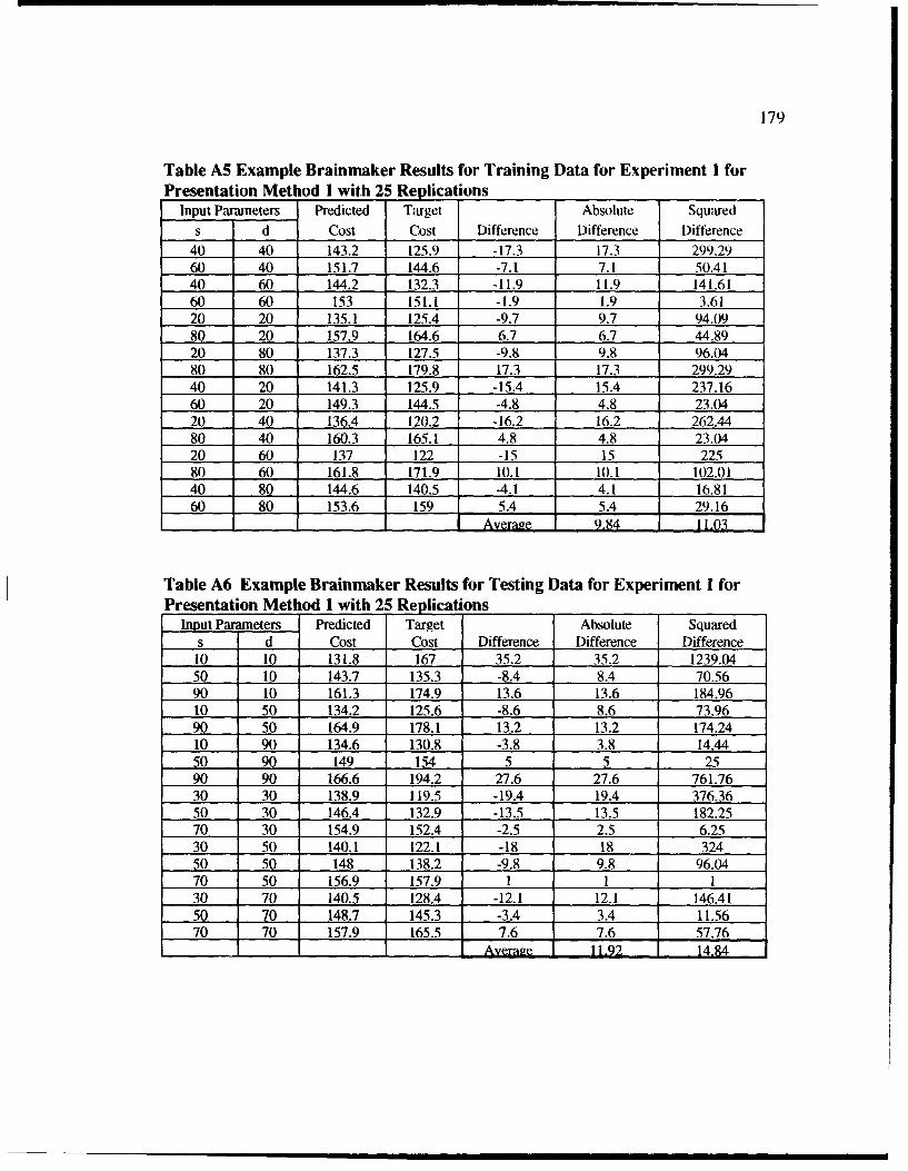
179
Table A5 Example Brainmaker Results for Training Data for Experiment I forPresentation Method I with 25 Replications
Input Parameters Predicted Target Absolute Squareds d Cost Cost Difference Difference Difference
40 40 143.2 125.9 -17.3 17.3 299.2960 40 151.7 144.6 -7.1 7.1 50.4140 60 144.2 132.3 -11.9 11.9 141.6160 60 153 151.1 -1.9 1.9 3.6120 20 135.1 125.4 -9.7 9.7 94.0980 20 157.9 164.6 6.7 6.7 44.8920 80 137.3 127.5 -9.8 9.8 96.0480 80 162.5 179.8 17.3 17.3 299.2940 20 141.3 125.9 -15.4 15.4 237.1660 20 149.3 144.5 -4.8 4.8 23.0420 40 136.4 120.2 -16.2 16.2 262.4480 40 160.3 165.1 4.8 4.8 23.0420 60 137 122 -15 15 22580 60 161.8 171.9 10.1 10.1 102.0140 80 144.6 140.5 -4.1 4.1 16.8160 80 153.6 159 5.4 5.4 29.16
Average 984 11,03
Table A6 Example Brainmaker Results for Testing Data for Experiment I forPresentation Method 1 with 25 Replications
Input Parameters Predicted Target Absolute Squareds d Cost Cost Difference Difference Difference10 10 131.8 167 35.2 35.2 1239.0450 10 143.7 135.3 -8.4 8.4 70.5690 10 161.3 174.9 13.6 13.6 184.9610 50 134.2 125.6 -8.6 8.6 73.9690 50 164.9 178.1 13.2 13.2 174.2410 90 134.6 130.8 -3.8 3.8 14.4450 90 149 154 5 5 2590 90 166.6 194.2 27.6 27.6 761.7630 30 138.9 119.5 -19.4 19.4 376.3650 30 146.4 132.9 -13.5 13.5 182.2570 30 154.9 152.4 -2.5 2.5 6.2530 50 140.1 122.1 -18 18 32450 50 148 138.2 -9.8 9.8 96.0470 50 156.9 157.9 1 1 130 70 140.5 128.4 -12.1 12.1 146.4150 70 148.7 145.3 -3.4 3.4 11.5670 70 157.9 165.5 7.6 7.6 57.76
Average 11.92 14.84
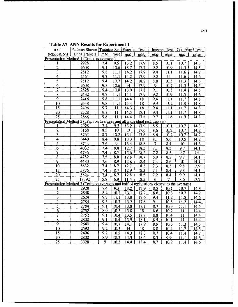
180)
Table A7 ANN Results for Experiment I# of Patterns Shown ITraining Set External Test I Internal Test Combined Test
SReplications] Until Trained mae I nnse mae rmse. mae rinse mae misePresentation Method I (Train c,n averages)
1 2928 7.4 9.5 13.2 17.9 8.5 10.1 10.7 14.32 2608 9.1 10.6 13.7 17.7 9.2 10.9 11.3 14.53 2512 9,8 11.1 14.2 17.9 9.4 11.1 11.6 14.74 2464 9.7 11.1 14.2 17.9 9.2 11 11.6 14.65 2512 9.4 10.7 14.2 18.2 8.8 10.5 11.3 14.66 2608 9.3 10.6 14 17.9 9 10.7 11.3 14.57 2528 9.4 10.8 13.9 17.8 9.1 10.8 11.4 14.58 2432 9.7 11.1 14.1 17.9 9.2 10.9 11.5 14.69 2416 9.8 11.1 14.4 18 9.4 11.1 11.7 14.810 2448 9.8 11.1 14.4 18 9.4 11.2 11.8 14.815 2496 9.7 11 14.3 18 9.4 11.1 11.7 14.820 2528 9.7 11 14.5 18.1 9,3 11.1 11.7 14.825 2688 9.8 11 14.4 17.8 9.7 11.6 11.9 14.8
Presentation Method 2 (Train on averages and all individual re lication s)1 2928 7.4 9.5 13.2 17.9 8.5 10.1 10.7 14.32 3168 8.3 10 13 17.6 8.6 10.2 10.7 14.23 3264 8.7 10.2 13.1 17.6 8.6 10.2 10.7 14.24 3440 8.4 9.8 13.3 18 8.1 9.6 10.5 14.25 3744 7.6 9 13.4 18.8 7 8.4 10 14.36 4032 7.4 8.8 12.7 18.5 7.1 8.5 9.7 14.17 4736 7.4 8.7 12.6 18.2 7.2 8.5 9.7 148 4752 7.5 8.8 12.8 18.7 6.9 8.2 9.7 14.19 4480 7.6 8.9 12.8 18.4 7.4 8.6 10 14.110 5632 7.4 8.7 12.7 18.3 7.3 8.3 9.8 13.915 5376 7.4 8.7 12.9 18.5 7.1 8.4 9.8 14.120 5824 7.4 8.7 12.8 18.5 7.2 8.4 9.9 14.125 13392 5.8 6.9 11.4 18.5 6 7 8.6 13.7
Presentation Method 3 (Train on averages and half of replications closest to the average)1 2928 7.4 9.5 13.2 17.9 8.5 10.1 10.7 14.32 2848 8.4 10.2 13.1 17.7 8.6 10.3 10.7 14.23 2624 9.7 11.1 13.8 17.6 9.4 11.2 11.5 14.64 2784 9.3 10.7 13.7 17.6 9.1 10.8 11.2 14.45 2784 9.1 10.4 13.8 18.1 8.7 10.3 11.1 14.56 2752 8.9 10.3 13.8 18 8.6 10.2 11 14.47 2752 9.1 10.4 13.5 17.8 8.8 10.4 11 14.48 2800 9.1 10.4 13.9 18.1 8.5 10.1 11 14.49 2640 9.4 10.7 14.1 17.9 8.9 10.6 11.3 14.510 2592 9.2 10.5 14 18 8.8 10.4 11.2 14.515 2496 9.2 10.5 14.3 18.3 8.7 10.4 11.4 14.720 2800 8.9 10.2 14.3 18.6 8.3 9.9 11.1 14.625 3328 9 10.3 14.4 18.4 8.7 10.2 11.4 14.6
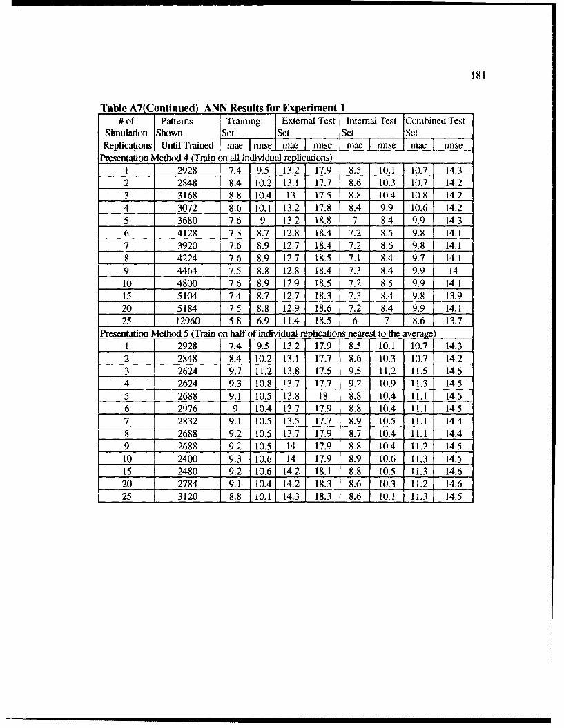
181
Table A7(Continued) ANN Results for Experiment I# of Patterns Training External Test Internal Test Combined Test
Simulation Shown Set Set Set SetReplications Until Trained F [mae I rmse maeI rmse ae I rmse mae I rmse
Presentation Method 4 (Train on all individual replications)1 2928 7.4 9.5 13.2 17.9 8.5 10.1 10.7 14.32 2848 8.4 10.2 13.1 17.7 8.6 10.3 10.7 14.23 3168 8.8 10.4 13 17.5 8.8 10.4 10.8 14.24 3072 8.6 10.1 13.2 17.8 8.4 9.9 10.6 14.25 3680 7.6 9 13.2 18.8 7 8.4 9.9 14.36 4128 7.3 8.7 12.8 18.4 7.2 8.5 9.8 14.17 3920 7.6 8.9 12.7 18.4 7.2 8.6 9.8 14.18 4224 7.6 8.9 12.7 18.5 7.1 8.4 9.7 14.19 4464 7.5 8.8 12.8 18.4 7.3 8.4 9.9 1410 4800 7.6 8.9 12.9 18.5 7.2 8.5 9.9 14.115 5104 7.4 8.7 12.7 18.3 7.3 8.4 9.8 13.920 5184 7.5 8.8 12.9 18.6 7.2 8.4 9.9 14.125 12960 5.8 6.9 11.4 18.5 6 7 8.6 13.7
Presentation Method 5 (Train on half of individual replications nearest to the average)1 2928 7.4 9.5 13.2 17.9 8.5 10.1 10.7 14.32 2848 8.4 10.2 13.1 17.7 8.6 10.3 10.7 14.23 2624 9.7 11.2 13.8 17.5 9.5 11.2 11.5 14.54 2624 9.3 10.8 13.7 17.7 9.2 10.9 11.3 14.55 2688 9.1 10.5 13.8 18 8.8 10.4 11.1 14.56 2976 9 10.4 13.7 17.9 8.8 10.4 11.1 14.57 2832 9.1 10.5 13.5 17.7 8.9 10.5 11.1 14.48 2688 9.2 10.5 13.7 17.9 8.7 10.4 11.1 14.49 2688 9.2 10.5 14 17.9 8.8 10.4 11.2 14.510 2400 9.3 10.6 14 17.9 8.9 10.6 11.3 14.515 2480 9.2 10.6 14.2 18.1 8.8 10.5 11.3 14.620 2784 9.1 10.4 14.2 18.3 8.6 10.3 11.2 14.625 3120 8.8 10.1 14.3 18.3 8.6 10.1 1 11.3 14.5

i n I I I
182
input number 1 2output number 1 4hidden 10 10
filename testfacts nn.tstfilename trainfacts k I ma 13.fctfilename teststats k lmaI 13.sta
learnrate 1.0000 50 1.0000 75 1.0000 90 1.0000learnlayer 1.0000 1.0000 1.0000traintol 0.1000 0.1000 0.8000 100testtol 0. 1000maxruns 5000smoothing 0.9000 0.9000 0.9000addhidden sequence 0.1 200
function hidden l sigmoid 0.0000 1.0000 0.0000 1function hidden2 sigmoid 0.0000 1.0000 0.0000 1function output sigmoid 0.0000 1.0000 0.0000 1
dictionary input s d
dictionary output tc dev min max
display network progress
scale input minimum05scale input maximum100 109scale output minimum55.0 25.0 0.0 106.0scale output maximum281.0 211.0 89.0 813.0
Figure A6 Initial Brainmaker Training File for Experiment 2 for PresentationMethod I with 25 Replications
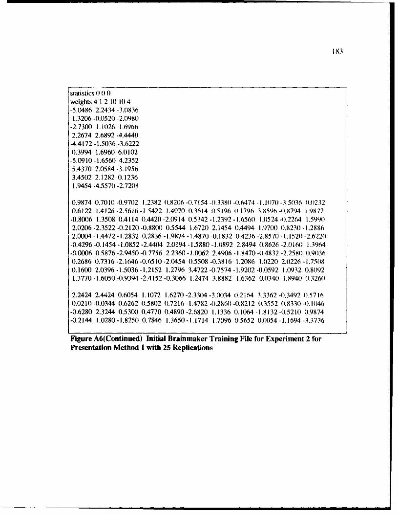
183
statistics 0 0 0weights 4 1 2 10 10 4-5.0486 2.2434 -3.08361.3206 -0.0520 -2.0980
-2.7300 1.1026 1.69662.2674 2.6892 -4.444)
-4.4172 -1.5036 -3.62220.3994 1.6960 6.0102
-5.0910 -1.6560 4.23525.4370 2.0584 -3.19563.4502 2.1282 0.12361.9454 -4.5570 -2.7208
0.9874 0.7010 -0.9702 1.2382 0.8206 -0.7154 -0.338() -0.6474 - 1.1070 -3.5036 0.02320.6122 1.4126 -2.5616 -1.5422 1.4970 0.3614 0.5196 0.1796 3.8596 -0.8794 1.9872-0.8006 1.3508 0.4114 0.4420 -2.0914 0.5342 -1.2392 -1.6560 1.0524 -0.2264 1.59902.0206-2.3522-0.2120-0.8800 0.5544 1.6720 2.1454 0.4494 1.9700 0.8230 -1.28862.0004 -1.4472 -1.2832 0.2836 -1.9874 -1.4870 -0.1832 0.4236 -2.8570 -1.1520 -2.6220-0.4296 -0.1454 -1.0852 -2.4404 2.0194 -1.5880 -1.0892 2.8494 0.8626 -2.0160 1.3964-0.0006 0.5876 -2.9450 -0.7756 2.2360 -1.0062 2.4906 -1.8470 -0.4832 -2.2580 0.90360.2686 0.7316 -2.1646 -0.6510-2.0454 0.5508 -0.3816 1.2086 1.0220 2.0226 -1.75080.1600 2.0396 -1.5036 -1.2152 1.2796 3.4722 -0.7574 -1.9202 -0.0592 1.0932 0.80921.3770 -1.6050 -0.9394 -2.4152 -0.3066 1.2474 3.8882 -1.6362 -0.0340 1.8940 0.3260
2.2424 2.4424 0.6054 1.1072 1.6270-2.3304 -3.0034 0.2i64 3.3362 -0.3492 0.57160.0210 -0.0344 0.6262 0.5802 0.7216 -1.4782 -0.2860 -0.8212 0.3552 0.8330 -0.1046
-0.6280 2.3244 0.5300 0.4770 0.4890 -2.6820 1.1336 0.1064 -1.8132 -0.5210 0.9874-0.2144 1.0280 -1.8250 0.7846 1.3650-1.1714 1.7096 0.5652 0.0054 -1.1694 -3.3736
Figure A6(Continued) Initial Brainmaker Training File for Experiment 2 forPresentation Method I with 25 Replications

184
input number 1 2output number 1 4hidden 10 10
filename trainfacts k I ma I 13.fctfilename testfacts nn.tstfilename teststats k Imal 13.sta
learnrate 1,000( 50 1.0000 75 1.(X)00 90 1.0000leamlayer 1.0000 1.0000 1.0000traintol 0.1000 0.1000 0.80(0 100tcsttol 0. 1000maxruns 2140smoothin& 0.9000 0.9000 0.9000addhidden sequence 0. 1 200
function hidden 1 sigmoid 0.0000 1.0000 0.0000 1function hidden2 sigmoid 0.0000 1.0000 0.0000 1function output sigmoid 0.0000 1.0000 0.0000 1
dictionary input s d
dictionary output tc dev min max
display network progress
scale input minimum05scale input maximum100 100scale output minimum55250106scale output maximum28121189813Figure A7 Trained Brainmaker File for Experiment 2 for PresentationMethod I with 25 Replications
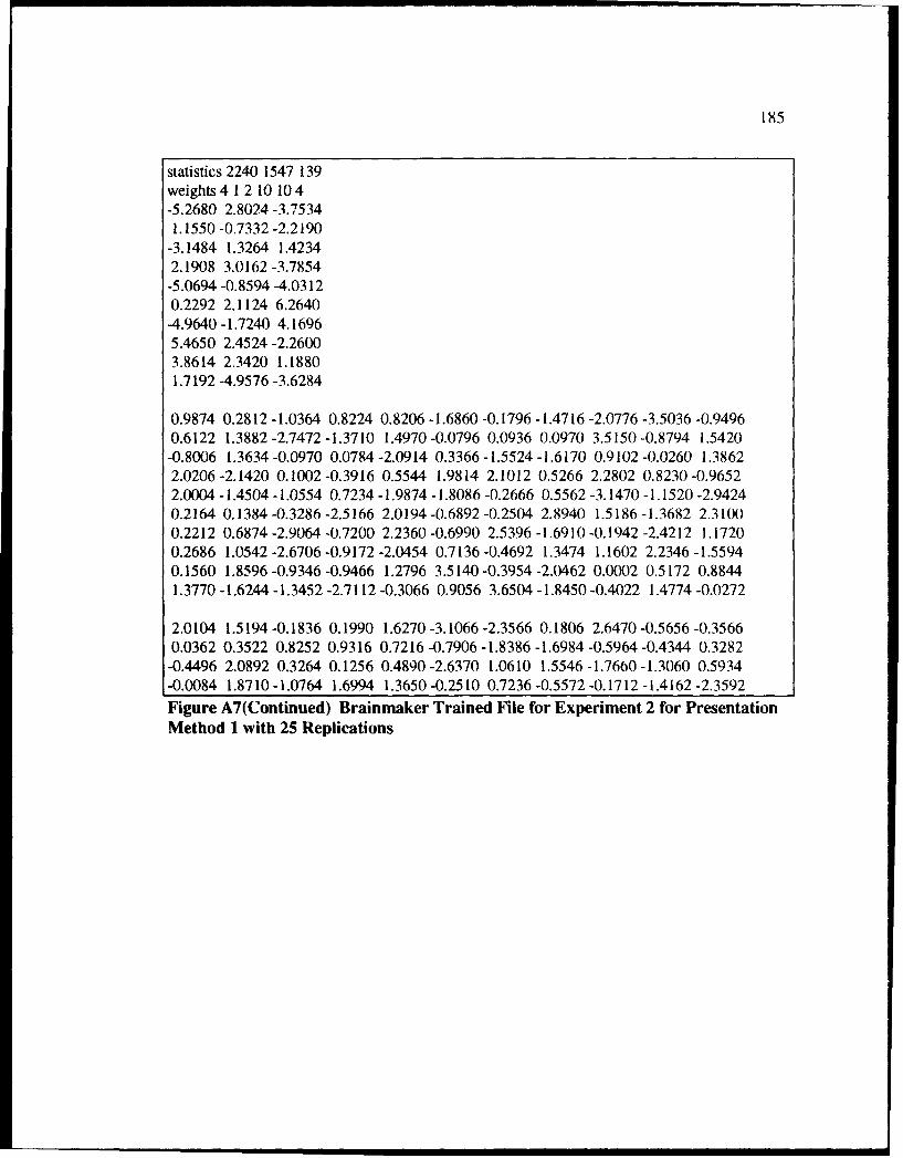
185
statistics 2240 1547 139weights 4 12 1010 4-5.2680 2.8024 -3.75341.1550 -0.7332 -2.2190
-3.1484 1.3264 1.42342.1908 3.0162 -3.7854
-5.0694 -0.8594 -4.03120.2292 2.1124 6.2640-4.9640 -1.7240 4.16965.4650 2.4524 -2.26003.8614 2.3420 1.18801.7192 -4.9576 -3.6284
0.9874 0.2812-1.0364 0.8224 0.8206 -1.6860 -0.1796 -1.4716 -2.0776 -3.5036 -0.94960.6122 1.3882 -2.7472 -1.3710 1.4970 -0.0796 0.0936 0.0970 3.5150 -0.8794 1.5420-0.8006 1.3634 -0.0970 0.0784 -2.0914 0.3366 -1.5524 -1.6170 0.9102 -0.0260 1.38622.0206 -2.1420 0.1002 -0.3916 0.5544 1.9814 2.1012 0.5266 2.2802 0.8230 -0.96522.0004 -1.4504 -1.0554 0.7234 -1.9874 -1.8086 -0.2666 0.5562 -3.1470 -1.1520 -2.94240.2164 0.1384 -0.3286 -2.5166 2.0194 -0.6892 -0.2504 2.8940 1.5186 -1.3682 2.3 1000.2212 0.6874 -2.9064 -0.7200 2.2360 -0.6990 2.5396 -1.6910 -0.1942 -2.4212 1.17200.2686 1.0542 -2.6706 -0.9172 -2.0454 0.7136 -0.4692 1.3474 1.1602 2.2346 -1.55940.1560 1.8596 -0.9346 -0.9466 1.2796 3.5140-0.3954-2.0462 0.0002 0.5172 0.88441.3770 -1.6244 -1.3452 -2.7112 -0.3066 0.9056 3.6504 -1.8450 -0.4022 1.4774 -0.0272
2.0104 1.5194 -0.1836 0.1990 1.6270 -3.1066 -2.3566 0.1806 2.6470 -0.5656 -0.35660.0362 0.3522 0.8252 0.9316 0.7216 -0.7906 -1.8386 -1.6984-0.5964-0.4344 0.3282
-0.4496 2.0892 0.3264 0.1256 0.4890 -2.6370 1.0610 1.5546 -1.7660-1.3060 0.5934-0.0084 1.8710-1.0764 1.6994 1.3650 -0.2510 0.7236 -0.5572 -0.1712 -1.4162 -2.3592
Figure A7(Continued) Brainmaker Trained File for Experiment 2 for PresentationMethod I with 25 Replications
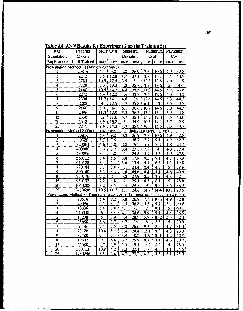
186
Table AS ANN Results for Experiment 2 on the Training Set# of Patterns Mean Cost Standard Minimum Maximum
Simulation Shown Deviation Cost CostReplications Until Trained mae Innse mae rmse Mae I rmse mae Tnmse
Presentation Method 1 (Train onAverages)1 20816 6.4 9.2 13.8 26.9 7.3 10.6 4.9 32.82 2272 6.5 12.81 4.7 37.1 8.7 13.1 5.4 43.9
3 2784 10.9 12.4 3.9 34 12.5 12.8 4.6 41.94 2528 6.3 13.3 4.2 35.3 8.7 13.6 5 435 2160 10.5 14.2 4.4 35.5 11.9 14.6 5.2 43.86 2272 6.4 12.2 4.6 35.3 7.5 12.6 5.3 43.57 2304 11.2 14.1 4.6 36 12.6 14.5 5.3 44.38 2288 4 12.5 4.7 35.8 6.1 13 5.5 44.29 2160 8.9 14 5.1 36.6 10.2 14.6 5.8 44.310 2096 11.3 12.9 5.3 36.3 13.2 13.4 5.9 44.815 2336 12 11.6 4.7 35.1 13.7 12.3 5.5 43.620 2048 8.9 13.8 5 34.9 10.3 14.1 5.7 42.925 2240 8.6 14.2 4.7 35.9 9.6 14.5 5.5 43.7
Presentation Method 2 (Train on averages and all individual renlications)1 20816 6.4 9.2 3.8 26.9 7.3 10.6 4.9 32.82 40320 5.7 7.5 4 38.7 7.7 9.1 4.9 42.33 320064 4.6 5.8 3.8 19.2 5.7 7.2 4.8 24.14 400080 6.3 3.2 3.8 23.3 7.2 4 4.8 27.45 480096 3.4 4.8 4 24.5 4.2 5.5 4.9 27.96 560112 8.4 8.5 3.8 17.8 9.5 9.1 4.7 23.97 640128 3.4 5.1 3.6 15.4 4.1 6.3 4.5 19.88 720144 7.7 3.8 4.1 24.4 8.4 4.5 5 28.99 800160 5.3 6.3 3.6 45.6 6.4 8.1 4.6 49.510 880176 7.2 3 3.8 27.9 8.5 3.9 4.8 32.115 960192 7.2 4.8 4 25.1 8.8 6.1 5 28.820 1040208 8.2 8.5 4.4 29.7 9 9.5 5.6 33.725 2480496 10.5 11.7 8.1 24.6 14.7 14.4 10.1 29.5
Presentation Method 3 (Train on averages & half of replications nearest average)1 20816 6.4 9.2 3.8 26.9 7.3 10.6 4.9 32.82 20096 4.5 8.4 4.5 36.8 5.8 9.7 5.4 40.63 10336 5.4 7.8 4.1 37 7 9.1 5 40.14 240048 9 8.4 4.1 34.6 9.9 9.1 4.8 38.95 13200 5 8.9 4.4 28.3 5.7 10.2 5.3 32.36 31680 6.6 7.7 4.2 26 8 8.6 5 30.97 9536 7.4 7.5 3.8 26.6 9.3 8.5 4.7 31.48 27120 10.4 8.1 3.4 24.4 12.1 9.3 4.3 28.39 32480 9.4 9.1 3.4 18.2 10.9 10.1 4.2 22.910 19392 7 6.6 3.7 25.8 8.7 8.1 4.6 30.715 55680 9.7 6.9 3.3 19.1 11.2 8.2 4 23.320 560112 10.8 4.2 3.3 20.1 11.6 4.9 4.1 24.525 1280256 3.5 7.4 4.7 20.2 4.2 8.6 6.1 25.9
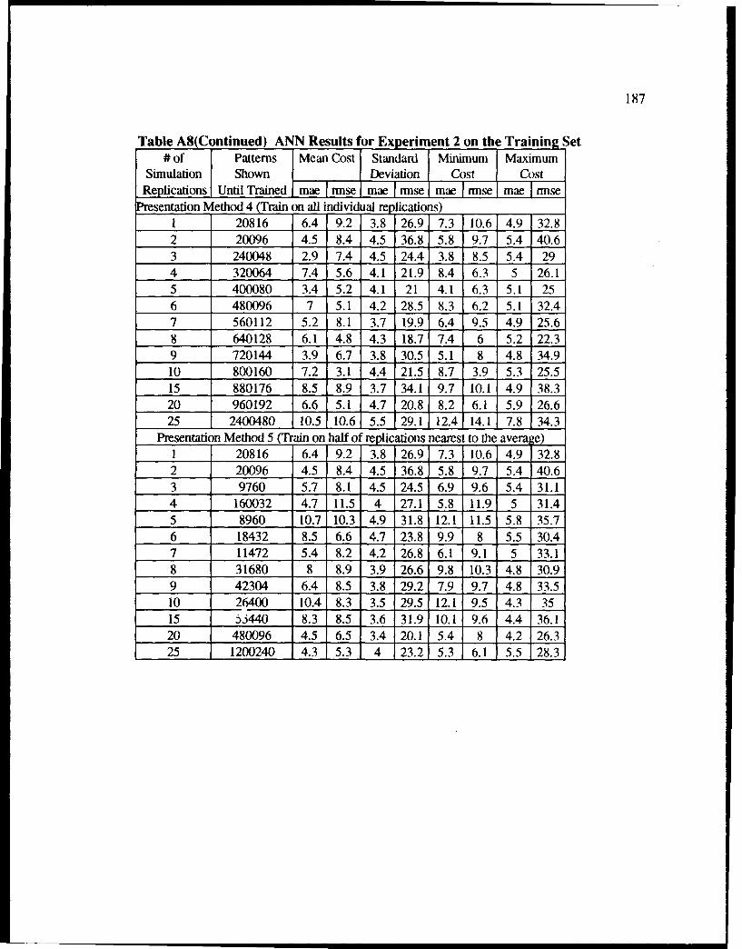
187
Table A8(Continued) ANN Results for Experiment 2 on the Training Set# of Patterns Mean Cost Standard Minimum Maximum
Simulation Shown Deviation Cost CostReplications Until Trained m ae I rinse mae inse mae in se
Presentation Method 4 (Train on all individual replications)1 20816 6.4 9.2 3.8 26.9 7.3 10.6 4.9 32.82 20096 4.5 8.4 4.5 36.8 5.8 9.7 5.4 40.63 240048 2.9 7.4 4.5 24.4 3.8 8.5 5.4 294 320064 7.4 5.6 4.1 21.9 8.4 6.3 5 26.15 400080 3.4 5.2 4.1 21 4.1 6.3 5.1 256 480096 7 5.1 4.2 28.5 8.3 6.2 5.1 32.47 560112 5.2 8.1 3.7 19.9 6.4 9.5 4.9 25.68 640128 6.1 4.8 4.3 18.7 7.4 6 5.2 22.39 720144 3.9 6.7 3.8 30.5 5.1 8 4.8 34.910 800160 7.2 3.1 4.4 21.5 8.7 3.9 5.3 25.515 880176 8.5 8.9 3.7 34.1 9.7 10.1 4.9 38.320 960192 6.6 5.1 4.7 20.8 8.2 6.1 5.9 26.625 2400480 10.5 10.6 5.5 29.1 12.4 14.1 7.8 34.3
Presentation Method 5 (Train on half of replications nearest to the avera ;e)1 20816 6.4 9.2 3.8 26.9 7.3 10.6 4.9 32.82 20096 4.5 8.4 4.5 36.8 5.8 9.7 5.4 40.63 9760 5.7 8.1 4.5 24.5 6.9 9.6 5.4 31.14 160032 4.7 11.5 4 27.1 5.8 11.9 5 31.45 8960 10.7 10.3 4.9 31.8 12.1 11.5 5.8 35.76 18432 8.5 6.6 4.7 23.8 9.9 8 5.5 30.47 11472 5.4 8.2 4.2 26.8 6.1 9.1 5 33.18 31680 8 8.9 3.9 26.6 9.8 10.3 4.8 30.99 42304 6.4 8.5 3.8 29.2 7.9 9.7 4.8 33.510 26400 10.4 8.3 3.5 29.5 12.1 9.5 4.3 3515 S5440 8.3 8.5 3.6 31.9 10.1 9.6 4.4 36.120 480096 4.5 6.5 3.4 20.1 5.4 8 4.2 26.325 1200240 4.3 5.3 4 23.2 5.3 6.1 5.5 28.3
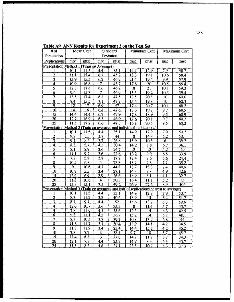
Ixx
Table A9 ANN Results for Experiment 2 on the Test Set# of Mean Cost Standard Minimum Cost Maximum Cost
Simulation Deviation
Replications mae rnse mae I rmse mae rinse mae misePresentation Method 1 (Train on Averages)
1 10.1 11.5 4.4 35.1 14.9 12.9 7.9 50.72 11.1 15.4 6.7 45.2 18.3 19.1 10.6 58.43 15.9 15.5 6.2 46.2 21.4 19.4 9.9 57.94 10.9 16.8 7 43.7 17.8 20 10.5 55.45 12.8 17.6 6.6 46.2 18 21 10.1 59.26 9.6 15.3 7 46.9 15.5 19.2 10.3 59.47 13.5 17.4 6.8 47.5 18.5 20.8 10 60.68 8.4 15.5 7.1 47.7 15.4 19.8 10 60.39 12 17 6.9 47 17.4 20.7 10.1 60.210 14 16 6.8 47.6 17.3 19.7 9.7 60.515 14.4 14.4 6.7 47.9 17.8 18.9 9.5 60.920 12.2 16.9 6.8 46.9 17.6 20.1 9.7 60.325 11.5 17.2 6.6 47.3 16.8 20.5 9.5 60.2
Presentation Method 2 (Train on averap es and individual re lications)1 10.1 11.5 4.4 35.1 14.9 12.9 7.9 50.72 9.7 11 3.8 44 18 14.3 6.2 53.13 9.1 8.2 3.7 26.8 15.9 10.5 6 39.24 8.3 5.7 4.3 30.4 14.2 8.8 6.7 36.15 8.1 8.9 2.6 24.7 12 12 4.2 296 11.1 9.2 3.6 22.6 13.2 9.9 6.5 33.57 7.2 5.7 2.8 17.8 12.4 7.6 5.6 24.48 10.5 6.8 4 28.8 13.7 9.3 7.1 35.29 9 10.6 4.7 44.8 13.7 15.3 7.4 49.910 10.8 5.5 3.4 28.1 16.3 7.8 4.9 32.615 12.4 6.9 2.9 26.6 18.9 8.1 4.1 32.720 11.8 10.6 4 30.3 16.4 11.1 5.2 3525 15.3 15.1 7.5 49.2 26.9 27.6 8.9 106
Presentation Method 3 (Train on averages and half of replications nearest to average)1 10.1 11.5 4.4 35.1 14.9 12.9 7.9 50.72 8.3 11.2 3.8 40.6 13.9 15 6.4 51.73 8.7 9.7 4.4 52 15.6 13.7 6.3 59.64 12.6 10.7 3.6 35.5 18 11.4 5.7 40.75 7.8 11.9 4.1 38.6 12.3 14 6.3 42.56 9.8 11.1 4.5 36.7 15.2 14 6.8 48.17 8.3 10.5 3.8 39.7 10.8 13.9 6.8 448 11.8 11.7 3.1 30.4 13.9 14.1 4.2 34.59 11.8 11.9 3.4 25.4 14.4 15.2 4.2 36.210 7.8 7.7 4 38.4 9.7 10 5.7 45.715 12.4 8.8 3 27.6 14.7 11.7 3.7 34.320 12.1 7.3 4.4 25.7 14.7 8.3 6.3 40.725 11.5 8.6 4.6 24.1 23.5 10.7 6.3 37.3
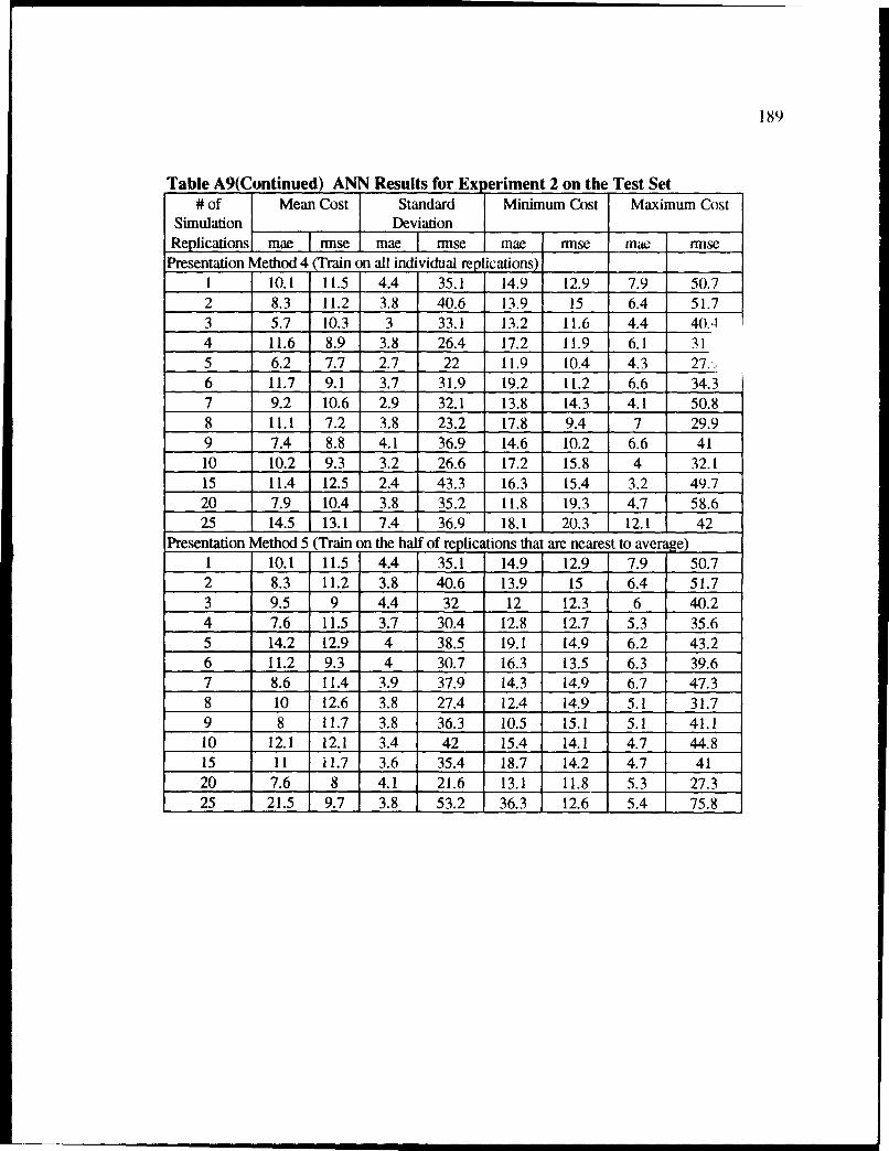
18X9
Table A9(Continued) ANN Results for Ex eriment 2 on the Test Set# of Mean Cost Standard Minimum Cost Maximum Cost
Simulation DeviationReplications ~mae rmse mae I nnse mae rmse mae rmse
Presentation Method 4 (Train on all individual replications)1 10.1 11.5 4.4 35.1 14.9 12.9 7.9 50.72 8.3 11.2 3.8 40.6 13.9 15 6.4 51.73 5.7 10.3 3 33.1 13.2 11.6 4.4 40.,14 11.6 8.9 3.8 26.4 17.2 11.9 6.1 315 6.2 7.7 2.7 22 11.9 10.4 4.3 27.,.6 11.7 9.1 3.7 31.9 19.2 11.2 6.6 34.37 9.2 10.6 2.9 32.1 13.8 14.3 4.1 50.88 11.1 7.2 3.8 23.2 17.8 9.4 7 29.99 7.4 8.8 4.1 36.9 14.6 10.2 6.6 4110 10.2 9.3 3.2 26.6 17.2 15.8 4 32.115 11.4 12.5 2.4 43.3 16.3 15.4 3.2 49.720 7.9 10.4 3.8 35.2 11.8 19.3 4.7 58.625 14.5 13.1 7.4 36.9 18.1 20.3 12.1 42
Presentation Method 5 (Train on the half of replications that are nearest to averae)1 10.1 11.5 4.4 35.1 14.9 12.9 7.9 50.72 8.3 11.2 3.8 40.6 13.9 15 6.4 51.73 9.5 9 4.4 32 12 12.3 6 40.24 7.6 11.5 3.7 30.4 12.8 12.7 5.3 35.65 14.2 12.9 4 38.5 19.1 14.9 6.2 43.26 11.2 9.3 4 30.7 16.3 13.5 6.3 39.67 8.6 11.4 3.9 37.9 14.3 14.9 6.7 47.38 10 12.6 3.8 27.4 12.4 14.9 5.1 31.79 8 11.7 3.8 36.3 10.5 15.1 5.1 41.110 12.1 12.1 3.4 42 15.4 14.1 4.7 44.815 11 11.7 3.6 35.4 18.7 14.2 4.7 4120 7.6 8 4.1 21.6 13.1 11.8 5.3 27.325 21.5 9.7 3.8 53.2 36.3 12.6 5.4 75.8

.vPPENDIX B
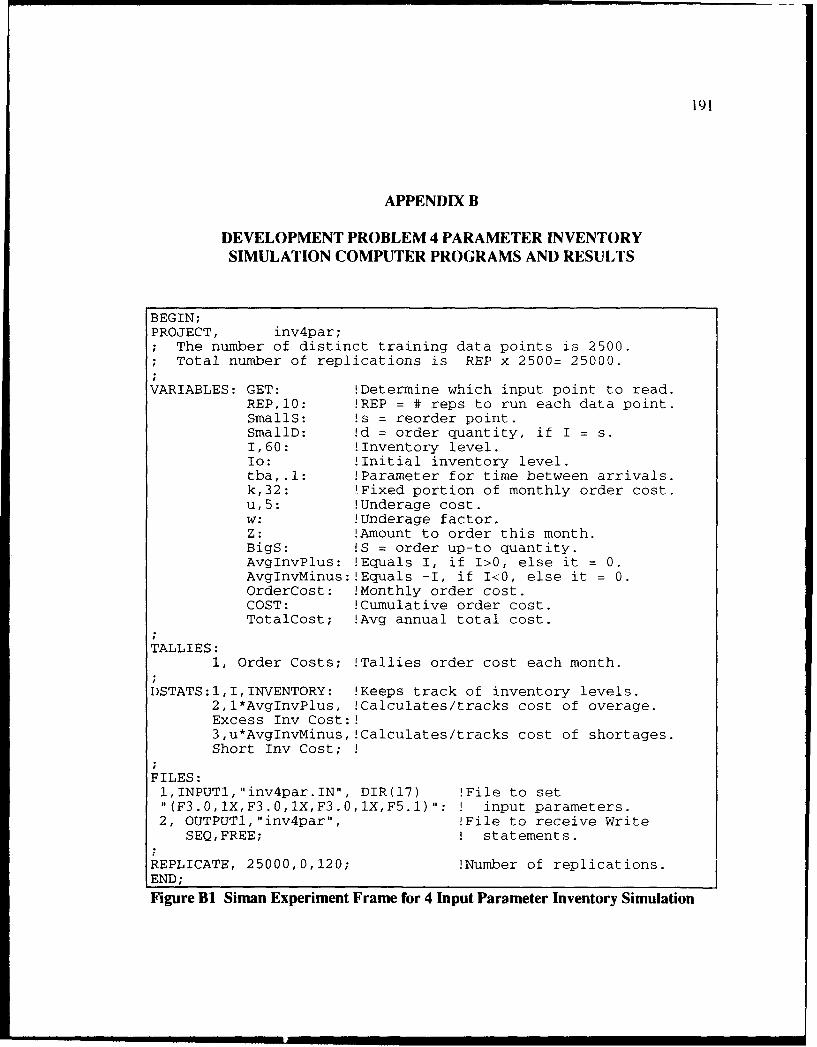
191
APPENDIX B
DEVELOPMENT PROBLEM 4 PARAMETER INVENTORYSIMULATION COMPUTER PROGRAMS AND RESULTS
BEGIN;PROJECT, inv4par;; The number of distinct training data points is 2500.; Total number of replications is REP x 2500= 25000.
VARIABLES: GET: !Determine which input point to read.REP, 10: !REP = # reps to run each data point.SmallS: !s = reorder point.SmallD: !d = order quantity, if I = s.1,60: !Inventory level.Io: !Initial inventory level.tba,.l: !Parameter for time between arrivals.k,32: !Fixed portion of monthly order cost.u,5: !Underage cost.w: !Underage factor.Z: !Amount to order this month.BigS: !S = order up-to quantity.AvgInvPlus: !Equals I, if I>0, else it = 0.AvgInvMinus:!Equals -I, if I<0, else it = 0.OrderCost: !Monthly order cost.COST: !Cumulative order cost.TotalCost; !Avg annual total cost.
TALLIES:1, Order Costs; !Tallies order cost each month.
I)STATS:I,I,INVENTORY: !Keeps track of inventory levels.2,1*AvgInvPlus, !Calculates/tracks cost of overage.Excess Inv Cost:!3,u*AvgInvMinus,!Calculates/tracks cost of shortages.Short Inv Cost;
FILES:l,INPUTl,"inv4par.IN", DIR(17) !File to set"(F3.0,lX,F3.0,iX,F3.0,1X, F5.1) ": ! input parameters.2, OUTPUTl,"inv4par", !File to receive Write
SEQ,FREE; ! statements.
REPLICATE, 25000,0,120; !Number of replications.END;Figure BI Siman Experiment Frame for 4 Input Parameter Inventory Simulation
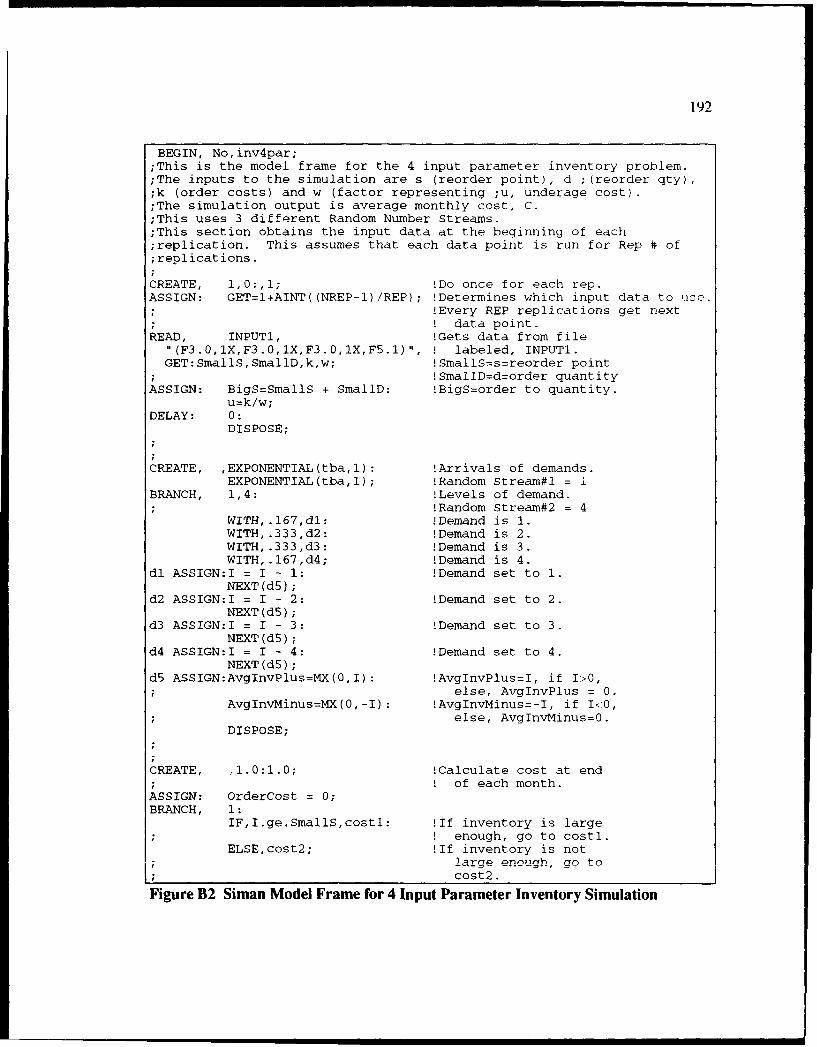
192
BEGIN, No,inv4par;;This is the model frame for the 4 input parameter inventory problem.;The inputs to the simulation are s (reorder point), d ;(reorder qty),;k (order costs) and w (factor representing ;u, underage cost).;The simulation output is average monthly cost, C.;This uses 3 different Random Number Streams.;This section obtains the input data at the beginning of each;replication. This assumes that each data point is run for Rep # of;replications.
CREATE, 1,0:,i; !Do once for each rep.ASSIGN: GET=I+AINT((NREP-I)/REP); !Determines which input data to use.
!Every REP replications get next! data point.
READ, INPUT1, !Gets data from file"(F3.0,lX,F3.0,1X,F3.0,1X,F5.1)", ! labeled, INPUT1.GET:SmallS,SmallD,k,w; !SmallS=s=reorder point
!SmallD=d=order quantityASSIGN: BigS=SmallS + SmallD: !BigS=order to quantity.
u=k/w;DELAY: 0:
DISPOSE;
CREATE, ,EXPONENTIAL(tba, 1): !Arrivals of demands.EXPONENTIAL(tba,l); !Random Stream#1 = 1
BRANCH, 1,4: !Levels of demand.!Random Stream#2 = 4
WITH,.167,dI: !Demand is 1.WITH,.333,d2: !Demand is 2.WITH,.333,d3: !Demand is 3.WITH,.167,d4; !Demand is 4.
dl ASSIGN:I = I - 1: !Demand set to 1.NEXT(dS);
d2 ASSIGN:I = I - 2: !Demand set to 2.NEXT(d5);
d3 ASSIGN:I = I - 3: !Demand set to 3.NEXT(dS);
d4 ASSIGN:I = I - 4: !Demand set to 4.NEXT(d5);
d5 ASSIGN:AvgInvPlus=MX(0,I): !AvgInvPlus=I, if I>0,else, AvgInvPlus = 0.
AvgInvMinus=MX(0,-I): !AvgInvMinus=-I, if I<0,else, AvgInvMinus=0.
DISPOSE;
CREATE, ,1.0:1.0; !Calculate cost at end! of each month.
ASSIGN: OrderCost = 0;BRANCH, 1:
IF,I.ge.SmallS,costl: !If inventory is large! enough, go to costl.
ELSE,cost2; !It inventory is notIArge9 enough, .otcost2. ,
Figure B2 Siman Model Frame for 4 Input Parameter Inventory Simulation
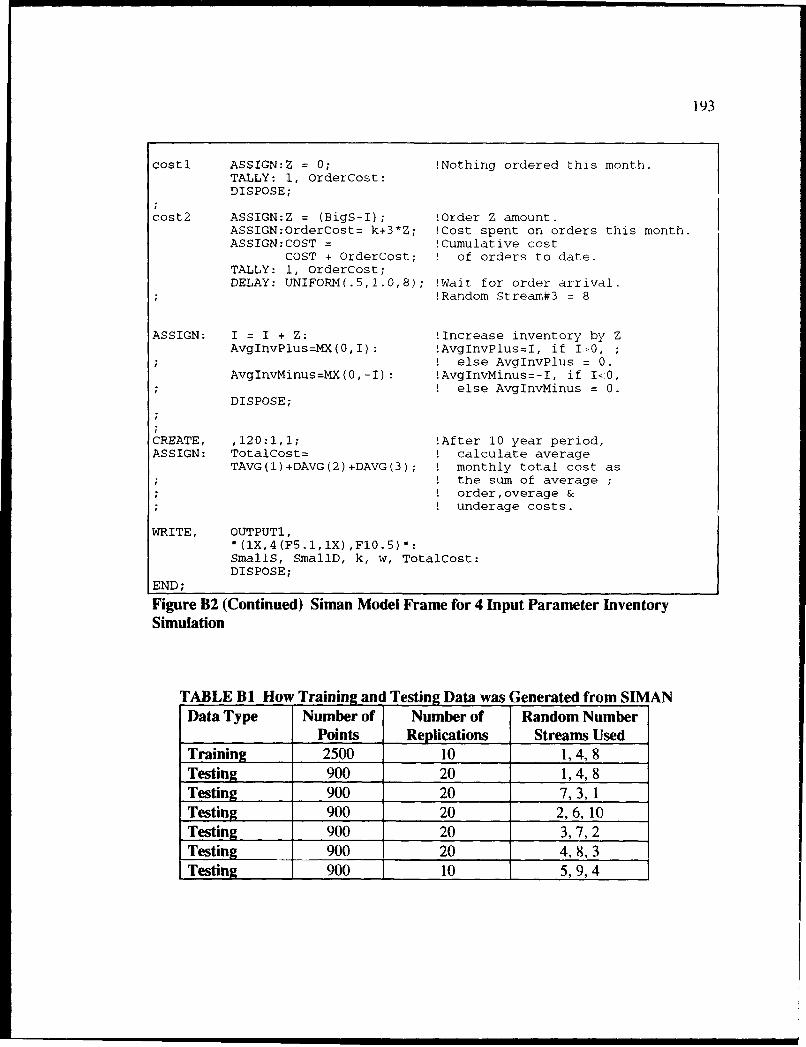
193
cost] ASSIGN:Z = 0; !Nothing ordered this month.TALLY: 1, OrderCost:DISPOSE;
cost2 ASSIGN:Z = (BigS-I); !Order Z amount.ASSIGN:OrderCost= k+3*Z; !Cost spent on orders this month.ASSIGN:COST = !Cumulative cost
COST + OrderCost; of ord-rs to date.TALLY: 1, OrderCost;DELAY: UNIFORM(.5,1.0,8); !Wait for order arrival.
!Random Stream#3 = 8
ASSIGN: I = I + Z: !Increase inventory by ZAvgInvPlus=MX(0,I) : !AvgInvPlus=I, if 1>0,
! else AvgInvPlus = 0.AvgInvMinus=MX(0,-I) : !AvgInvMinus=-I, if I0,
else AvgInvMinus = 0.DISPOSE;
CREATE, ,120:1,1; !After 10 year period,ASSIGN: TotalCost= . calculate average
TAVG(1)+DAVG(2)+DAVG(3); monthly total cost asthe sum of average;order,overage &underage costs.
WRITE, OUTPUT1,"C(lX,4(F5.l,lX),Fl0.5)":SmallS, SmallD, k, w, TotalCost:DISPOSE;
END;
Figure B2 (Continued) Siman Model Frame for 4 Input Parameter InventorySimulation
TABLE B1 How Training and Testing Data was Generated from SIMANData Type Number of Number of Random Number
Points Replications Streams UsedTraining 2500 10 1, 4, 8Testing 900 20 1, 4, 8Testing 900 20 7, 3, 1Testing 900 20 2, 6, 10Testing 900 20 3, 7, 2Testing 900 20 4, 8, 3Testing 900 10 5,9,4
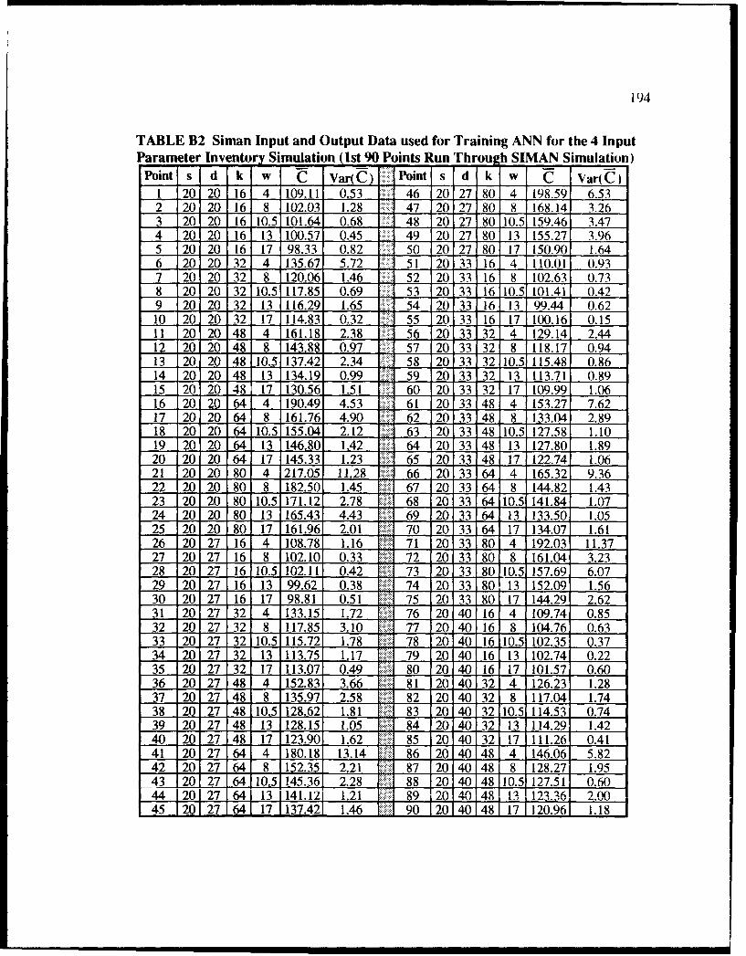
194
TABLE B2 Siman Input and Output Data used for Training ANN for the 4 InputParameter Inventor Simulation (Ist 90 Points Run Through SIMAN Simulation)
Point s d k -w C Var(C) Point s d k w C Var(C)1 20 20 16 4 109.11 0.53 1 46 20 27 80 4 198.59 6.532 20 20 16 8 102.03 1.28 47 20 27 80 8 168.14 3.263 20 20 16 10.5 101.64 0.68 -ý 48 20 27 80 10.5 159.46 3.474 20 20 16 13 100.57 0.45 49 20 27 80 13 155.27 3.965 20 20 16 17 98.33 0.82 50 20 27 80 17 150.90 1.646 20 20 32 4 135.67 5.72 51 20 33 16 4 110.01 0.937 20 20 32 8 120.06 1.46 1 52 20 33 16 8 102.63 0.738 20 20 32 10.5 117.85 0.69 1 53 20 33 16 10.5 101.41 0.429 20 20 32 13 116.29 1.65 1 54 20 33 16 13 99.44 0.6210 20 20 32 17 114.83 0.32 55 20 33 16 17 100.16 0.1511 20 20 48 4 161.18 2.38 56 20 33 32 4 129.14 2.4412 20 20 48 8 143.88 0.97 57 20 33 32 8 118.17 0.9413 20 20 48 10.5 137.42 2.34 i 58 20 33 32 10.5 115.48 0.8614 20 20 48 13 134.19 0.99 . 59 20 33 32 13 113.71 0.8915 20 20 48 17 130.56 1.51 60 20 33 32 17 109.99 1.0616 20 20 64 4 190.49 4.53 . 61 20 33 48 4 153.27 7.6217 20 20 64 8 161.76 4.90 . 62 20 33 48 8 133.04 2.8918 20 20 64 10.5 155.04 2.12 .. 63 20 33 48 10.5 127.58 1.1019 20 20 64 13 146.80 1.42 :.j 64 20 33 48 13 127.80 1.8920 20 20 64 17 145.33 1.23 65 20 33 48 17 122.74 1.0621 20 20 80 4 217.05 11.28 66 20 33 64 4 165.32 9.3622 20 20 80 8 182.50 1.45 67 20 33 64 8 144.82 1.4323 20 20 80 10.5 171.12 2.78 68 20 33 64 10.5 141.84 1.0724 20 20 80 13 165.43 4.43 69 20 33 641 13 133.50 1.0525 20 20 80 17 161.96 2.01 70 20 33 64 17 134.07 1.6126 20 27 16 4 108.78 1.16 71 20 33 80 4 192.03 11.3727 20 27 16 8 102.10 0.33 72 20 33 80 8 161.04 3.2328 20 27 16 10.5 102.11 0.42 73 20 33 80 10.5 157.69 6.0729 20 27 16 13 99.62 0.38 74 20 33 80 13 152.09 1.5630 20 27 16 17 98.81 0.51 75 20 33 801 17 144.29 2.6231 20 27 32 4 133.15 1.72 76 20 40 16 4 109.74 0.8532 20 27 32 8 117.85 3.10 77 20 40 16 8 104.76 0.6333 20 27 32 10.5 115.72 1.78 78 20 40 16 10.5 102.35 0.3734 20 27 32 13 113.75 1.17 79 20 40 16 13 102.74 0.2235 20 27 32 17 113.07 0.49 80 20 40 16 17 101.57 0.6036 20 27 48 4 152.83 3.66 81 20 40 32 4 126.23 1.2837 20 27 48 8 135.97 2.58 82 20 40 32 8 117.04 1.7438 20 27 48 10.5 128.62 1.81 83 20 40 32 10.5 114.53 0.7439 20 27 48 13 128.15 1.05 84 20 40 32 13 114.29 1.4240 20 27 48 17 123.90 1.62 85 20 40 32 17 111.26 0.4141 20 27 64 4 180.18 13.14 86 20 40 48 4 146.06 5.8242 20 27 64 8 152.35 2.21 87 20 40 48 8 128.27 1.9543 20 27 64 10.5 145.36 2.28 88 20 40 48 10.5 127.51 0.6044 20127. 64 13 1141.12 1.21 1. 89 220 401 A• 13 123.36 2.0045 20 27 64 17 1137.42 1.46 9 20 4048 17 1120.96 1.18
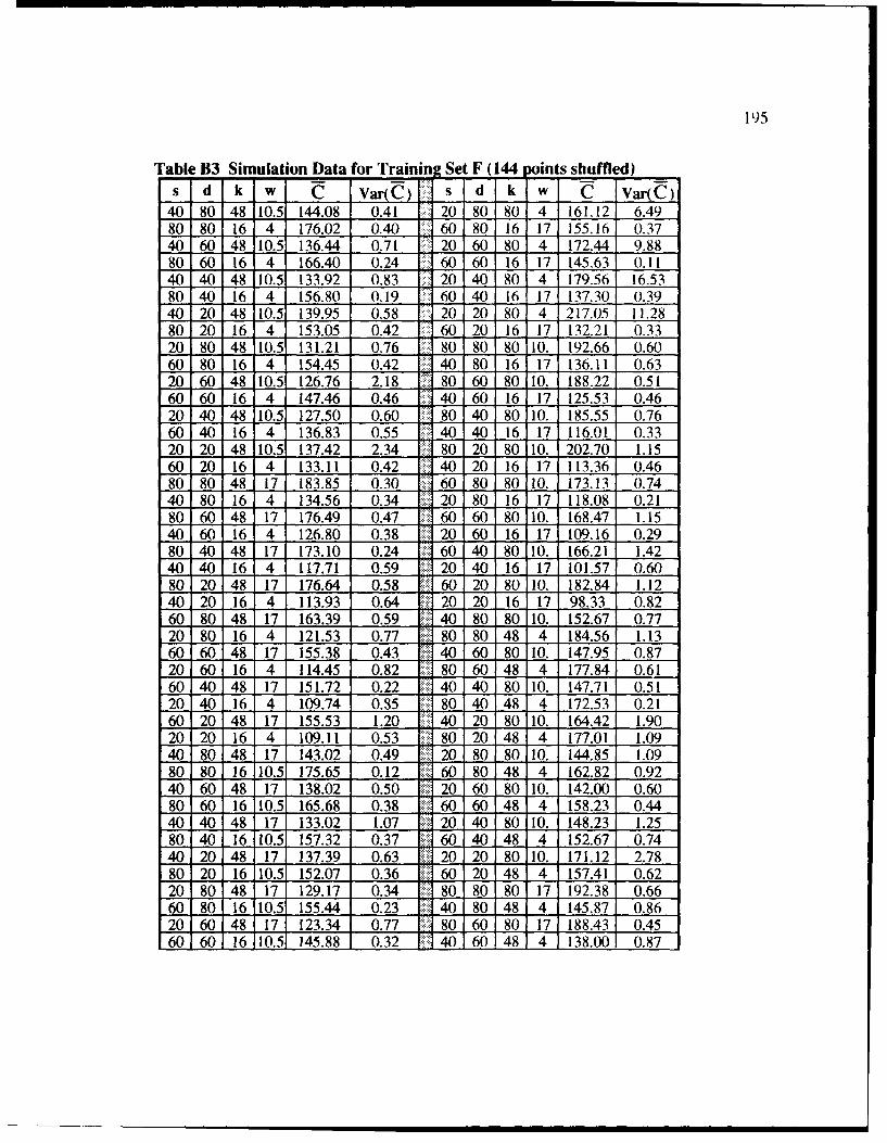
195
Table B3 Simulation Data for Trainin Set F (144 ints shuffled)S d k w C Var(C) s d k w C Var(C)
40 80 48 10.5 144.08 0.41 20 80 80 4 161.12 6.4980 80 16 4 176.02 0.40 60 80 16 17 155.16 0.3740 60 48 10.5 136.44 0.71 20 60 80 4 172.44 9.8880 60 16 4 166.40 0.24 60 60 16 17 145.63 0.1140 40 48 10.5 133.92 0.83 20 40 80 4 179.56 16.5380 40 16 4 156.80 0.19 60 40 16 17 137.30 0.3940 20 48 10.5 139.95 0.58 20 20 80 4 217.05 11.2880 20 16 4 153.05 0.42 60 20 16 17 132.21 0.3320 80 48 10.5 131.21 0.76 1 80 80 80 10. 192.66 0.6060 80 16 4 154.45 0.42 40 80 16 17 136.11 0.6320 60 48 10.5 126.76 2.18 80 60 80 10. 188.22 0.5160 60 16 4 147.46 0.46 40 60 16 17 125.53 0.4620 40 48 10.5 127.50 0.60 80 40 80 10. 185.55 0.7660 40 16 4 136.83 0.55 40 40 16 17 116.01 0.3320 20 48 10.5 137.42 2.34 80 20 80 10. 202.70 1.1560 20 16 4 133.11 0.42 40 20 16 17 113.36 0.4680 80 48 17 183.85 0.30 60 80 80 10. 173.13 0.7440 80 16 4 134.56 0.34 20 80 16 17 118.08 0.2180 60 48 17 176.49 0.47 60 60 80 10. 168.47 1.1540 60 16 4 126.80 0.38 20 60 16 17 109.16 0.2980 40 48 17 173.10 0.24 60 40 80 10. 166.21 1.4240 40 16 4 117.71 0.59 20 40 16 17 101.57 0.6080 20 48 17 176.64 0.58 60 20 80 10. 182.84 1.1240 20 16 4 113.93 0.64 20 20 16 17 98.33 0.8260 80 48 17 163.39 0.59 40 80 80 10. 152.67 0.7720 80 16 4 121.53 0.77 80 80 48 4 184.56 1.1360 60 48 17 155.38 0.43 40 60 80 10. 147.95 0.8720 60 16 4 114.45 0.82 80 60 48 4 177.84 0.6160 40 48 17 151.72 0.22 40 40 80 10. 147.71 0.5120 40 16 4 109.74 0.85 80 40 48 4 172.53 0.2160 20 48 17 155.53 1.20 40 20 80 10. 164.42 1.9020 20 16 4 109.11 0.53 80 20 48 4 177.01 1.0940 80 48 17 143.02 0.49 20 80 80 10. 144.85 1.0980 80 16 10.5 175.65 0.12 60 80 48 4 162.82 0.9240 60 48 17 138.02 0.50 20 60 80 10. 142.00 0.6080 60 16 10.5 165.68 0.38 60 60 48 4 158.23 0.4440 40 48 17 133.02 1.07 20 40 80 10. 148.23 1.2580 40 16 10.5 157.32 0.37 60 40 48 4 152.67 0.7440 20 48 17 137.39 0.63 20 20 80 10. 171.12 2.7880 20 16 10.5 152.07 0.36 60 20 48 4 157.41 0.6220 80 48 17 129.17 0.34 80 80 80 17 192.38 0.6660 80 16 10.5 155.44 0.23 40 80 48 4 145.87 0.8620 60 48 17 123.34 0.77 80 60 80 17 188.43 0.4560 60 16 10.5 145,88 0.32- 40 60 48 4 138.00 0.87
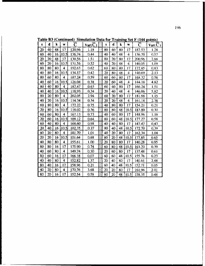
196
Table B3 (Continued) Simulation Data for Trainin Set F (144 oints)s d k w C Var(C) s d k w C Var(C)
20 40 48 17 120.96 1.18 80 40 80 17 187.53 1.2860 40 16 10.5 136.74 0.44 40 40 48 4 136.70 0.5720 20 48 17 130.56 1.51 80 20 80 17 200.96 2.6860 20 16 10.51 131.56 0.52 40 20 48 4 140.05 1.0980 80 80 4 192.63 0.62 60 80 80 17 172.85 0.8340 80 16 10.5 134.57 0.42 20 80 48 4 140.69 2.1380 60 80 4 187.24 0.59 60 60 80 17 168.32 0.5640 60 16 10.5 126.04 0.38 20 60 48 4 144.18 4.8280 40 80 4 187.47 0.63 60 40 80 17 166.24 1.5140 40 16 10.5 118.93 0.34 20 40 48 4 146.06 5.8280 20 80 4 202.05 2.94 60 20 80 17 181.98 1.1540 20 16 10.5 114.34 0.34 20 20 48 4 161.18 2.3860 80 80 4 172.22 0.75 40 80 80 17 154.21 0.2120 80 16 10.5 118.02 0.36 80 80 48 10.5 183.80 0.3060 60 80 4 167.13 0.73 40 60 80 17 148.96 1.1620 60 16 10.5 109.12 0.64 80 60 48 10.5 177.27 0.5860 40 80 4 168.60 0.98 40 40 80 17 147.47 0.4320 40 16 10.5 102.35 0.37 80 40 48 10.5 172.70 0.3960 20 80 4 181.70 1.01 40 20 80 17 162.34 1.0420 20 16 10.5 101.64 0.68 80 20 48 10.5 177.85 0.65
40 80 80 4 155.61 1.00 20 80 80 17 140.28 0.9580 80 16 17 175.90 0.74 60 80 48 10.5 163.70 0.3940 60 80 4 149.74 0.30 20 60 80 17 137.48 0.61.
......80 60 16 17 166.38 0.07 iiiiil60 60 48 10.5 155.76 0.23
40 40 80 4 152.82 1.37 20 40 80 17 140.61 2.4880 40 16 17 158.96 0.21 60 40 48 10.5 152.71 0.0540 20 80 4 170.76 3.68 20 20 80 17 161.96 2.0180 20 16 17 152.54 0.58 60 20 48 10.5 158.35 0.48
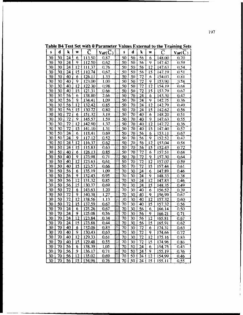
197
Table B4 Test Set with 0 Parameter Values External to the Training SetsS d k w C Var(C) S d k w C Var(C)
30 30 24 6 113.50 0.87 50 50 56 6 148.00 0.7030 30 24 9 112.50 0.62 50 50 56 9 147.42 0.5930 30 24 12 111.37 0.76 50 50 56 12 147.63 0.5430 30 24 15 110.74 0.67 50 50 56 15 147.19 0.5130 30 40 6 126.11 1.33 50 50 72 6 154.03 0.8130 30 40 9 123.00 1.00 50 50 72 9 153.90 '.5830 30 40 12 122.30 0.98 50 50 72 12 154.19 0.6830 30 40 15 121.31 0.66 50 50 72 15 153.79 0.6730 30 56 6 138.80 2.66 50 70 24 6 143.30 0.4730 30 56 9 134.41 1.09 50 70 24 9 142.75 0.3630 30 56 12 132.42 0.85 50 70 24 12 142.79 0.4930 30 56 15 130.72 0.80 50 70 24 15 142.62 0.5630 30 72 6 151.32 3.19 50 70 40 6 148.20 0.5130 30 72 9 145.57 1.59 50 70 40 9 147.63 0.5530 30 72 12 142.90 1.37 50 70 40 12 147.72 0.3630 30 72 15 141.10 1.31 50 70 40 15 147.40 0.5730 50 24 6 118.41 0.69 50 70 56 6 153.11 0.6730 50 24 9 117.12 0.52 50 70 56 9 152.52 0.4730 50 24 12 116.37 0.62 50 70 56 12 153.04 0.5830 50 24 15 115.83 0.63 50 70 56 15 152.43 0.7230 50 40 6 126.13 0.85 50 70 72 6 157.51 0.6830 50 40 9 123.98 0.71 50 70 72 9 157.30 0.6430 50 40 12 123.63 0.61 50 70 72 12 157.07 0.5930 50 40 15 123.57 0.66 50 70 72 15 157.44 0.6130 50 56 6 135.19 1.09 .. 70 30 24 6 147.89 0.4630 50 56 9 132.43 0.95 70 30 24 9 148.33 0.3830 50 56 12 131.32 0.85 70 30 24 12 147.83 0.4630 50 56 15 130.37 0.69 70 30 24 15 148.35 0.4930 50 72 6 143.63 1.20 70 30 40 6 156.52 0.3930 50 72 9 140.38 1.27 70 30 40 9 156.99 0.6730 50 72 12 138.56 1.13 /0 30 40 12 157.32 0.6030 50 72 15 137.59 0.67 70 30 40 15 157.32 0.5630 70 24 6 125.26 0.67 70 30 56 6 166.14 0.5030 70 24 9 125.08 0.56 70 30 56 9 166.21 0.7130 70 24 12 123.84 0.34 70 30 56 12 165.81 0.6730 70 24 15 123.88 0.44 70 30 56 15 165.91 0.6230 70 40 6 132.06 0.83 70 30 72 6 174.31 0.6330 70 40 9 130.43 0.63 70 30 72 9 174.66 0.7230 70 40 12 129.33 0.61 .... 70 30 72 12 175.16 0.8330 70 40 15 129.48 0.55 70 30 72 15 174.96 0.8630 70 56 6 138.39 1.05 70 50 24 6 154.75 0.4330 70 56 9 136.17 0.71 70 50 24 9 155.19 0.3630 70 56 12 135.02 0.69 70 50 24 12 154.99 0.4630 70 56 15 134.96 0.76 70 50 24 15 155.11 0.55
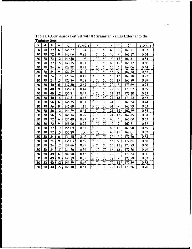
198
Table B4(Continued) Test Set with 0 Parameter Values External to theTraining Sets
s d k w C Var(C) S d k w C Var(C)
30 70 72 6 145.22 1.74 70 50 40 6 161.21 0.5330 70 72 9 142.06 0.82 70 50 40 9 161.17 0.6430 70 72 12 140.56 1.06 70 50 40 12 161.51 0.5430 70 72 15 140.15 0.91 70 50 40 15 161.12 0.5050 30 24 6 128.28 0.41 70 50 56 6 168.06 0.5450 30 24 9 127.89 0.47 70 50 56 9 167.30 0.6250 30 24 12 128.54 0.45 70 50 56 12 167.18 0.7250 30 24 15 127.86 0.38 70 50 56 15 167.89 0.7950 30 40 6 137.80 0.62 70 50 72 6 173.69 0.7550 30 40 9 136.63 0.47 70 50 72 9 173.57 0.6950 30 40 12 136.81 0.43 70 50 72 12 173.20 0.7350 30 40 15 137.31 0.68 70 50 72 15 174.22 0.6350 30 56 6 146.35 0.91 70 70 24 6 163.34 0.4450 30 56 9 145.69 1.13 70 70 24 9 162.73 0.5550 30 56 12 146.29 0.64 70 70 24 12 162.89 0.5550 30 56 15 146.34 0.79 70 70 24 15 162.85 0.3850 30 72 6 155.40 0.87 70 70 40 6 167.60 0.5350 30 72 9 155.90 0.92 70 70 40 9 167.81 0.5750 30 72 12 155.09 0.85 70 70 40 12 167.90 0.5550 30 72 15 155.28 1.00 70 70 40 15 168.01 0.5750 50 24 6 134.80 0.46 70 70 56 6 172.76 0.5250 50 24 9 135.03 0.59 70 70 56 9 172.64 0.6650 50 24 12 134.66 0.39 70 70 56 12 172.83 0.6050 50 24 15 134.76 0.36 70 70 56 15 172.70 0.7950 50 40 6 141.58 0.43 70 70 72 6 177.34 0.6050 50 40 9 141.18 0.55 70 70 72 9 177.58 0.5750 50 40 12 141.39 0.66 70 70 72 12 177.59 0.5550 50 40 15 141.40 0.51 70 70 72 15 177.26 0.76

199
nlf5.detinput number 1 4output number 1 1hidden 5 5filename trainfacts m lb.fctfilename testfacts ml d.tstfilename teststats n I f5.stafilename trainstats n I f5 stslearnrate 1.0000 50 1.0000 75 1.0000 90 1.0000learnlayer 1.0000 1.0000 1.0000traintol 0.0200 0.0200 0.8000 100testtol 0.0200maxruns 750smoothing 0.9000 0.9000 0.9000testruns 1function hidden 1 sigmoid 0.0000 1.0000 0.0000 1.0000function hidden2 sigmoid 0.0000 1.0000 0.0000 1.0000function output sigmoid 0.0000 1.0000 0.0000 1.0000dictionary input s d k wdictionary output tcscale input minimum2.0000 2.0000 0.000 1.5000scale input maximum98.000 98.000 96.000 19.500scale output minimum45.680scale output maximum554.17statistics 0 0 0weights 4 14 5 5 1-2.3886 1.0226 -0.0402 -1.6250 -2.11460.8540 1.3142 1.7564 2.0830 -3.4422
-3.4214 -1.1646 -2.8056 0.3094 1.31364.6552 -3.9432 -1.2824 3.2806 4.21121.5944 -2.4754 2.6724 1.6484 0.0960
1.3756 -3.2220 -1.9236 1.3374 0.9496 -1.31401.6766 1.1110 -0.9690 -0.4576 -0.8770 -1.4986
4.7440 0.0316 0.8292 1.9126 -3.4686 -2.08842.0272 0.4896 0.7032 0.2432 5.2260-1.19082.6908-1.0842 1.8292 0.5574 0.5990-2.8316
0.7232 -1.6782 -2.2422 1.4250 -0.3066 2.1650Figure B3 Initial BrainMaker Training File for Predicting Mean Cost

200
n1f5.netinput number 1 4output number 1 1hidden 5 5filename trainfacts m I b.fctfilename testfacts m Id.tstfilename teststats n5.stafilename trainstats n5.stsleamrate 1.0000 50 1.0000 75 1.0000 90 1.0000learnlayer 1.0000 1.0000 1.0000traintol 0.0200 0.0200 0.8000 100testtol 0.0200maxruns 58smoothing 0.9000 0.9000 0.9000testruns 58function hidden 1 sigmoid 0.0000 1.0000 0.0000 1.0000function hidden2 sigmoid 0.0000 1.0000 0.0000 1.0000function output sigmoid 0.0000 1.0000 0.0000 1.0000dictionary input s d k wdictionary output tcoutputfile nlf5.out number none number number none 000scale input minimum2.0000 2.0000 0.000 1.5000scale input maximum98.000 98.000 96.000 19.500scale output minimum45.680scale output maximum554.17statistics 83520 11670 58weights 4 1 4 5 5 1-1.6830 -3.2044 1.3186 -0.1604 -0.8976-7.9998 -5.1952 -4.6116 -5.1224 -5.5262-3.3516 -1.9562 -0.4174 -0.1970 1.95827.2766 0.5708 -2.2656 3.9482 0.80047.9994 6.5356 7.9994 4.3016 7.9994
1.4716 -7.9998 -4.6276 -0.4610 0.4430 -1.86447.3596 -4.3536 1.9686 -7.9998 -7.9998 -7.9998-4.9430 0.0456 2.2070 3.2404 -2.6000 -0.92742.0272 -7.9998 -3.1106 -7.9998 -7.7506 -7.99982.6908 -0.8932 4.8906 -7.9998 -7.9998 -7.99985.6852 0.9166 -2.9240 4.2820 1.7166 -0.27 10
Figure B4 Trained BrainMaker File for Predicting Mean Cost Using Replications
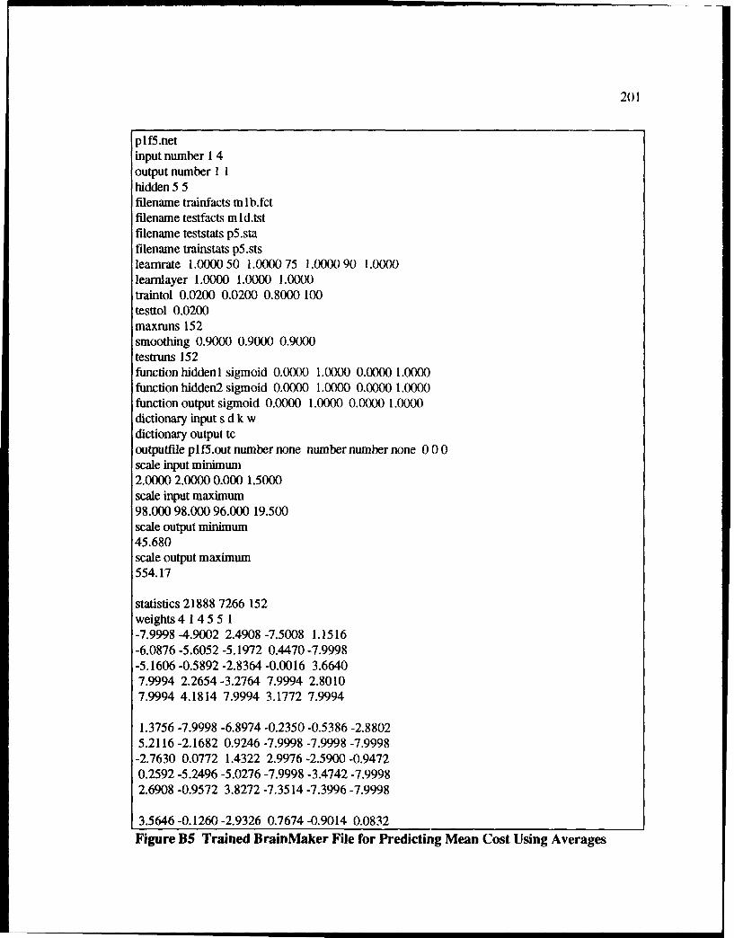
i 2() I
20)
pIf5.netinput number 1 4output number 1 1hidden 5 5filename trainfacts m lb.fctfilename testfacts m ld.tstfilename teststats pS.stafilename trainstats p5.stsleamrate 1.0000 50 1.0000 75 1.0000 90 1.0000learlayer 1.0000 1.0000 1.0000traintol 0.0200 0.0200 0.8000 100testtol 0.0200maxruns 152smoothing 0.9000 0.9000 0.9000testruns 152function hidden I sigmoid 0.0000 1.0000 0.0000 1.0000function hidden2 sigmoid 0.0000 1.0000 0.0000 1.0000function output sigmoid 0.0000 1.0000 0.0000 1.0000dictionary input s d k wdictionary output tcoutputfile plf5.out number none number number none 000scale input minimum2.0000 2.0000 0.000 1.5000scale input maximum98.000 98.000 96.000 19.500scale output minimum45.680scale output maximum554.17
statistics 21888 7266 152weights 4 1 4 5 5 1-7.9998 -4.9002 2.4908 -7.5008 1.1516-6.0876 -5.6052 -5.1972 0.4470 -7.9998-5.1606 -0.5892 -2.8364 -0.0016 3.66407.9994 2.2654-3.2764 7.9994 2.80107.9994 4.1814 7.9994 3.1772 7.9994
1.3756 -7.9998 -6.8974 -0.2350 -0.5386 -2.88025.2116 -2.1682 0.9246 -7.9998 -7.9998 -7.9998-2.7630 0.0772 1.4322 2.9976 -2.5900 -0.94720.2592 -5.2496 -5.0276 -7.9998 -3.4742 -7.99982.6908 -0.9572 3.8272 -7.3514 -7.3996 -7.9998
3.5646 -0.1260 -2.9326 0.7674 -0.9014 0.0832Figure B5 Trained BrainMaker File for Predicting Mean Cost Using Averages
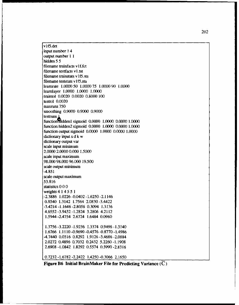
202
v I f.detinput number 14output number 1 1hidden 5 5filename trainfacts v lf.fctfilename testfacts v .tstfilename trainstats v lf5.stsfilename teststats v I f5.stalearnrate 1.0000 50 1.0000 75 1.0000 90 1.0000learnlayer 1.0000 1.0000 1.0000traintol 0.0020 0.0020 0.8000 100testtol 0.0020maxruns 750smoothing 0.9000 0.9000 0.9000testrunskfunctiontiddenl sigmoid 0.0000 1.0000 0.0000 1.0000function hidden2 sigmoid 0.0000 1.0000 0.0000 1.0000function output sigmoid 0.0000 1.0000 0.0000 1.0000dictionary input s d k wdictionary output varscale input minimum2.0000 2.0000 0.000 1.5000scale input maximum98.000 98.000 96.000 19.500scale output minimum-4.851scale output maximum53.816statistics 0 0 0weights 4 14 5 5 1-2.3886 1.0226 -0.0402 -1.6250 -2.11460.8540 1.3142 1.7564 2.0830 -3.4422-3.4214-1.1646 -2.8056 0.3094 1.31364.6552 -3.9432 -1.2824 3.2806 4.21121.5944 -2.4754 2.6724 1.6484 0.0960
1.3756 -3.2220 -1.9236 1.3374 0.9496 -1.31401.6766 1.1110 -0.9690 -0.4576 -0.8770 -1.4986
-4.7440 0.0316 0.8292 1.9126 -3.4686 -2.08842.0272 0.4896 0.7032 0.2432 5.2260 -1.19082.6908 -1.0842 1.8292 0.5574 0.5990 -2.8316
0.7232 -1.6782 -2.2422 1.4250 -0.3066 2.1650
Figure B6 Initial BrainMaker File for Predicting Variance (C)
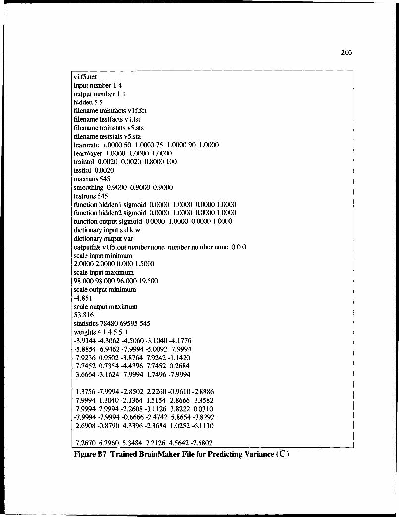
203
v I f5.netinput number 1 4output number 11hidden 5 5filename trainfacts v lf.fctfilename testfacts v l.tstfilename trainstats v5.stsfilename teststats v5.staleamrate 1.0000 50 1.0000 75 1.0000 90 1.0000learnlayer 1.0000 1.0000 1.0000traintol 0.0020 0.0020 0.8000 100testtol 0.0020maxruns 545smoothing 0.9000 0.9000 0.9000testruns 545function hidden 1 sigmoid 0.0000 1.0000 0.0000 1.0000function hidden2 sigmoid 0.0000 1.0000 0.0000 1.0000function output sigmoid 0.0000 1.0000 0.0000 1.0000dictionary input s d k wdictionary output varoutputfile v If5.out number none number number none 0 0 0scale input minimum2.0000 2.0000 0.000 1.5000scale input maximum98.000 98.000 96.000 19.500scale output minimum-4.851scale output maximum53.816statistics 78480 69595 545weights 4 1 4 5 5 1-3.9144 -4.3062 -4.5060 -3.1040 -4.1776-5.8854 -6.9462 -7.9994 -5.0092 -7.99947.9236 0.9502 -3.8764 7.9242 -1.14207.7452 0.7354 -4.4396 7.7452 0.26843.6664 -3.1624 -7.9994 1.7496 -7.9994
1.3756 -7.9994 -2.8502 2.2260 -0.9610 -2.88867.9994 1.3040-2.1364 1.5154 -2.8666 -3.35827.9994 7.9994 -2.2608 -3.1126 3.8222 0.0310-7.9994 -7.9994 -0.6666 -2.4742 5.8654 -3.82922.6908 -0.8790 4.3396 -2.3684 1.0252 -6.1110
7.2670 6.7960 5.3484 7.2126 4.5642 -2.6802
Figure B7 Trained BrainMaker File for Predicting Variance (C)

APPENDIX C
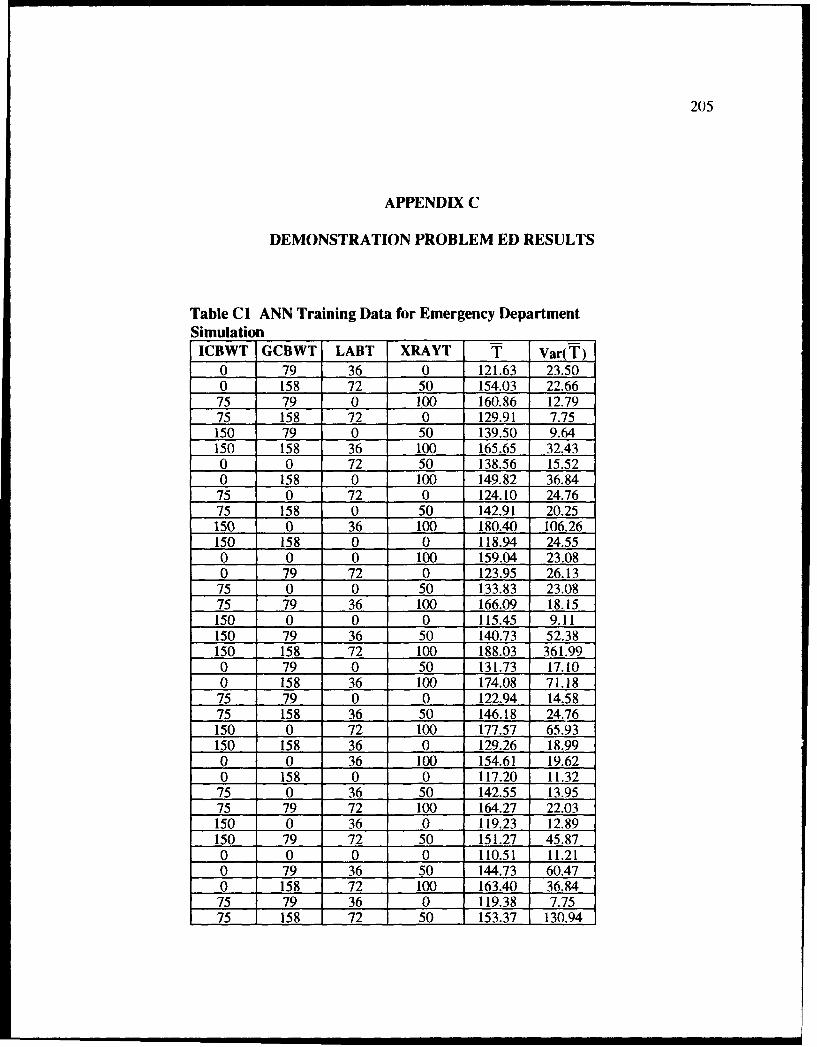
205
APPENDIX C
DEMONSTRATION PROBLEM ED RESULTS
Table CI ANN Training Data for Emergency DepartmentSimulation
ICBWT GCBWT LABT XRAYT T Var(T)
0 79 36 0 121.63 23.500 158 72 50 154.03 22.6675 79 0 100 160.86 12.7975 158 72 0 129.91 7.75150 79 0 50 139.50 9.64150 158 36 100 165.65 32.430 0 72 50 138.56 15.520 158 0 100 149.82 36.84
75 0 72 0 124.10 24.7675 158 0 50 142.91 20.25150 0 36 100 180.40 106.26150 158 0 0 118.94 24.550 0 0 100 159.04 23.080 79 72 0 123.95 26.13
75 0 0 50 133.83 23.0875 79 36 100 166.09 18.15150 0 0 0 115.45 9.11150 79 36 50 140.73 52.38150 158 72 100 188.03 361.990 79 0 50 131.73 17.100 158 36 100 174.08 71.18
75 79 0 0 122.94 14.5875 158 36 50 146.18 24.76150 0 72 100 177.57 65.93150 158 36 0 129.26 18.990 0 36 100 154.61 19.620 158 0 0 117.20 11.32
75 0 36 50 142.55 13.9575 79 72 100 164.27 22.03150 0 36 0 119.23 12.89150 79 72 50 151.27 45.870 0 0 0 110.51 11.210 79 36 50 144.73 60.470 158 72 100 163.40 36.84
75 79 36 0 119.38 7.7575 158 72 50 153.37 130.94
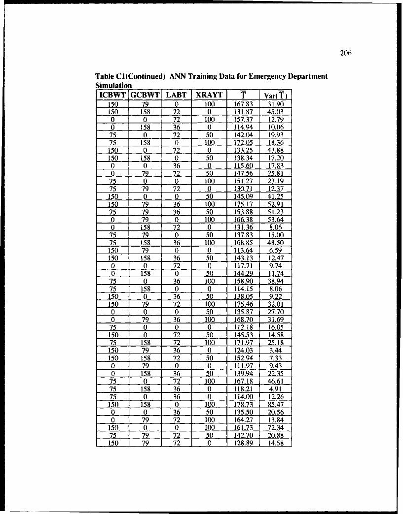
206
Table CI(Continued) ANN Training Data for Emergency DepartmentSimulationICBWT GCBWT LABT XRAYT T Var(T)
150 79 0 100 167.83 31.90150 158 72 0 131.87 45.030 0 72 100 157.37 12.790 158 36 0 114.94 10.0675 0 72 50 142.04 19.9375 158 0 100 172.05 18.36150 0 72 0 133.25 43.88150 158 0 50 138.34 17.200 0 36 0 115.60 17.830 79 72 50 147.56 25.8175 0 0 too 151.27 23.19
75 79 72 0 130.71 12.37150 0 0 50 145.09 41.25150 79 36 100 175.17 52.9175 79 36 50 153.88 51.230 79 0 100 166.38 53.640 158 72 0 131.36 8.0675 79 0 50 137.83 15.0075 158 36 100 168.85 48.50150 79 0 0 113.64 6.59150 158 36 50 143.13 12.470 0 72 0 117.71 9.740 158 0 50 144.29 11.74
75 0 36 100 158.90 38.9475 158 0 0 114.15 8.06150 0 36 50 138.05 9.22150 79 72 100 175.46 32.010 0 0 50 135.87 27.700 79 36 100 168.70 31.6975 0 0 0 112.18 16.05150 0 72 50 145.53 14.5875 158 72 100 171.97 25.18150 79 36 0 124.03 3.44150 158 72 50 152.94 7.330 79 0 0 111.97 9.430 158 36 50 139.94 22.3575 0 72 100 167.18 46.6175 158 36 0 118.21 4.9175 0 36 0 114.00 12.26150 158 0 100 178.73 85.470 0 36 50 135.50 20.560 79 72 100 164.27 13.84
150 0 0 100 161.73 72.3475 79 72 50 142.70 20.88150 79 72 0 128.89 14.58
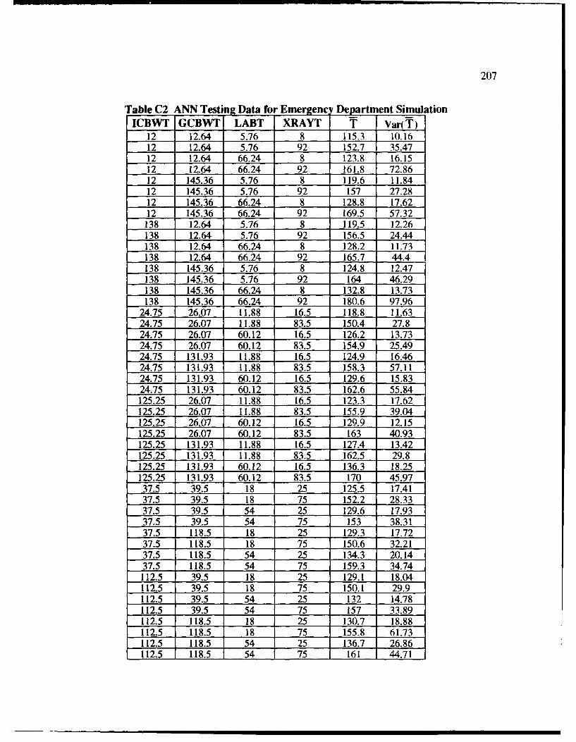
207
Table C2 ANN Testing Data for Emergency Department SimulationICBWT GCBWT LABT XRAYT T Var(T)
12 12.64 5.76 8 115.3 10.1612 12.64 5.76 92 152.7 35.4712 12.64 66.24 8 123.8 16.1512 12.64 66.24 92 161.8 72.8612 145.36 5.76 8 119.6 11.8412 145.36 5.76 92 157 27.2812 145.36 66.24 8 128.8 17.6212 145.36 66.24 92 169.5 57.32138 12.64 5.76 8 119.5 12.26138 12.64 5.76 92 156.5 24.44138 12.64 66.24 8 128.2 11.73138 12.64 66.24 92 165.7 44.4138 145.36 5.76 8 124.8 12.47138 145.36 5.76 92 164 46.29138 145.36 66.24 8 132.8 13.73138 145.36 66.24 92 180.6 97.96
24.75 26.07 11.88 16.5 118.8 11.6324.75 26.07 11.88 83.5 150.4 27.824.75 26.07 60.12 16.5 126.2 13.7324.75 26.07 60.12 83.5 154.9 25.4924.75 131.93 11.88 16.5 124.9 16.4624.75 131.93 11.88 83.5 158.3 57.1124.75 131.93 60.12 16.5 129.6 15.8324.75 131.93 60.12 83.5 162.6 55.84125.25 26.07 11.88 16.5 123.3 17.62125.25 26.07 11.88 83.5 155.9 39.04125.25 26.07 60.12 16.5 129.9 12.15125.25 26.07 60.12 83.5 163 40.93125.25 131.93 11.88 16.5 127.4 13.42125.25 131.93 11.88 83.5 162.5 29.8125.25 131.93 60.12 16.5 136.3 18.25125.25 131.93 60.12 83.5 170 45.97
37.5 39.5 18 25 125.5 17.4137.5 39.5 18 75 152.2 28.3337.5 39.5 54 25 129.6 17.9337.5 39.5 54 75 153 38.3137.5 118.5 18 25 129.3 17.7237.5 118.5 18 75 150.6 32.2137.5 118.5 54 25 134.3 20.1437.5 118.5 54 75 159.3 34.74112.5 39.5 18 25 129.1 18.04112.5 39.5 18 75 150.1 29.9112.5 39.5 54 25 132 14.78112.5 39.5 54 75 157 33.89112.5 118.5 18 25 130.7 18.88112.5 118.5 18 75 155.8 61.73112.5 118.5 54 25 136.7 26.86112.5 118.5 54 75 161 44.71
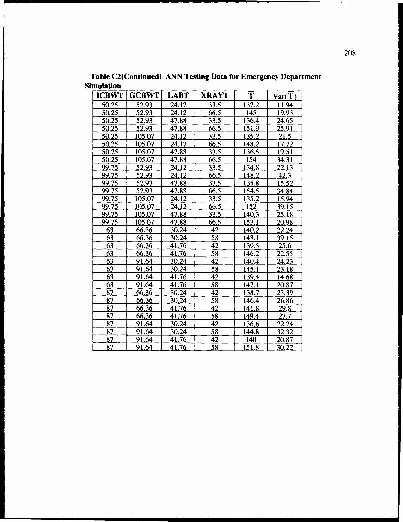
208
Table C2(Continued) ANN Testing Data for Emergency DepartmentSimulation
ICBWT GCBWT LABT XRAYT T Var(T)50.25 52.93 24.12 33.5 132.2 11.9450.25 52.93 24.12 66.5 145 19.9350.25 52.93 47.88 33.5 136.4 24.6550.25 52.93 47.88 66.5 151.9 25.9150.25 105.07 24.12 33.5 135.2 21.550.25 105.07 24.12 66.5 148.2 17.7250.25 105.07 47.88 33.5 136.5 19.5150.25 105.07 47.88 66.5 154 34.3199.75 52.93 24.12 33.5 134.8 22.1399.75 52.93 24.12 66.5 148.2 42.399.75 52.93 47.88 33.5 135.8 15.5299.75 52.93 47.88 66.5 154.5 34.8499.75 105.07 24.12 33.5 135.2 15.9499.75 105.07 24.12 66.5 152 39.1599.75 105.07 47.88 33.5 140.3 25.1899.75 105.07 47.88 66.5 153.1 20.98
63 66.36 30.24 42 140.2 22.2463 66.36 30.24 58 148.1 39.1563 66.36 41.76 42 139.5 25.663 66.36 41.76 58 146.2 22.5563 91.64 30.24 42 140.4 24.2363 91.64 30.24 58 145.1 23.1863 91.64 41.76 42 139.4 14.6863 91.64 41.76 58 147.1 20.8787 66.36 30.24 42 138.7 23.3987 66.36 30.24 58 146.4 26.8687 66.36 41.76 42 141.8 29.887 66.36 41.76 58 149.4 27.787 91.64 30.24 42 136.6 22.2487 91.64 30.24 58 144.8 32.3287 91.64 41.76 42 140 20.8787 91.64 41.76 58 151.8 30.22
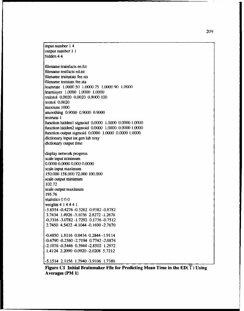
209
input number 1 4output number 1 1hidden 4 4
filename trainfacts ee.fctfilename tesffacts ed.tstfilename trainstats fee.stsfilename teststats fee.staleamrate 1.0000 50 1.0000 75 1.0000 90 1.0000learnlayer 1.0000 1.0000 1.0000traintol 0.0020 0.0020 0.8000 100testtol 0.0020maxruns 1000smoothing 0.9000 0.9000 0.9000testruns 1function hiddenl sigmoid 0.0000 1.0000 0.0000 1.0000function hidden2 sigmoid 0.0000 1.0000 0.0000 1.0000function output sigmoid 0.0000 1.0000 0.0000 1.0000dictionary input int gen lab xraydictionary output time
display network progressscale input minimum0.0000 0.0000 0.000 0.0000scale input maximum150.000 158.000 72.000 100.000scale output minimum102.72scale output maximum195.76statistics 0 0 0weights 4 1 444 1-3.8554 -0.4276 -0.3262 0.9382 -0.87823.7434 1.4926 -3.1036 2.8272 -1.2676
-0.3316 -3.0782 -1.7292 0.1736 -0.75122.7450 4.5422 -4.1044 -0.1690 -2.7670
-0.4850 1.8116 0.0434 0.2844 -1.9114-0.6790 -0.2360 -2.7194 0.7742 -2.0874-2.1076 -0.5446 0.3944 -2.8502 1.29721.4124 2.2090 0.0920 -2.0208 5.7212
-5.1514 2.1156 1.7940-3.9106 1.7380
Figure CI Initial Brainmaker File for Predicting Mean Time in the ED(T) UsingAverages (PM 1)
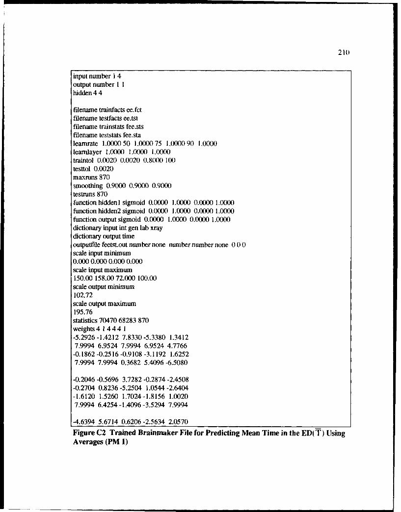
210
input number 1 4output number 11hidden 4 4
filename trainfacts ee.fctfilename testfacts ee.tstfilename trainstats fee.stsfilename teststats fee.staleamrate 1.0000 50 1.0000 75 1.0000 90 1.0000learnlayer 1.0000 1.0000 1.0000traintol 0.0020 0.0020 0.8000 100testtol 0.0020maxruns 870smoothing 0.9000 0.9000 0.9000testruns 870function hidden 1 sigmoid 0.0000 1.0000 0.0000 1.0000function hidden2 sigmoid 0.0000 1.0000 0.0000 1.0000function output sigmoid 0.0000 1.0000 0.0000 1.0000dictionary input int gen lab xraydictionary output timeoutputfile feetst.out number none number number none 0 0 0scale input minimum0.000 0.000 0.000 0.000scale input maximum150.00 158.00 72.000 100.00scale output minimum102.72scale output maximum195.76statistics 70470 68283 870weights4 1 444 1-5.2926-1.4212 7.8330-5.3380 1.34127.9994 6.9524 7.9994 6.9524 4.7766
-0.1862 -0.2516 -0.9108 -3.1192 1.62527.9994 7.9994 0.3682 5.4096 -6.5080
-0.2046 -0.5696 3.7282 -0.2874 -2.4508-0.2704 0.8236 -5.2504 1.0544 -2.6404-1.6120 1.5260 1.7024-1.8156 1.00207.9994 6.4254 -1.4096 -3.5294 7.9994
-4.6394 5.6714 0.6206-2.5634 2.0570
Figure C2 Trained Brainmaker File for Predicting Mean Time in the ED(T) UsingAverages (PM 1)

211
input number 1 4output number 1 1hidden 4 4
filename trainfacts ed.fctfilename testfacts ed.tstfilename trainstats fed.stsfilename teststats fed.sta
leamrate 1.000050 1.0000 75 1.000090 1.0000learnlayer 1.0000 1.0000 1.0000traintol 0.0020 0.0020 0.8000 100testtol 0.0020maxruns 1000smoothing 0.9000 0.9000 0.9000testruns 1function hidden 1 sigmoid 0.0000 1.0000 0.0000 1.0000function hidden2 sigmoid 0.0000 1.0000 0.0000 1.0000function output sigmoid 0.0000 1.0000 0.0000 1.0000dictionary input int gen lab xraydictionary output timedisplay network progressscale input minimum0.0000 0.0000 0.000 0.0000scale input maximum150.000 158.000 72.000 100.000scale output minimum69.01scale output maximum366.57statistics 0 0 0weights 4 1 4 44 1-3.8554 -0.4276 -0.3262 0.9382 -0.87823.7434 1.4926 -3.1036 2.8272 -1.2676
-0.3316 -3.0782 -1.7292 0.1736 -0.75122.7450 4.5422 -4.1044 -0.1690 -2.7670
-0.4850 1.8116 0.0434 0.2844 -1.9114-0.6790 -0.2360 -2.7194 0.7742 -2.0874-2.1076 -0.5446 0.3944 -2.8502 1.29721.4124 2.2090 0.0920-2.0208 5.7212
-5.1514 2.1156 1.7940-3.9106 1.7380
Figure C3 Initial Brainmaker File for Predicting Mean Time in the ED(T) UsingIndividual Replications (PM 4)

212
input number 1 4output number I Ihidden 4 4
filename trainfacts ed.fctfilename testfacts ed.tstfilename trainstats fed.stsfilename teststats fed.staleamrate 1.0000 50 1.000( 75 1.0000 90 1.0000learnlayer 1.0000 1.0000 1.0000traintol 0.0020 0.0020 0.8000 1(0testtol 0.0020maxruns 259smoothing 0.9000 0.9000 0.9000tesruns 259function hiddeni sigmoid 0.0000 1.0000 0.0000 1.0000function hidden2 sigmoid 0.0000 1.0000 0.0000 1.0000function output sigmoid 0.0000 1.0000 0.0000 1.0000dictionary input int gen lab xraydictionary output timeoutputfile fedtst.out number none number number none 0 0 0scale input minimum0.000 0.000 0.000 0.000scale input maximum150.00 158.00 72.000 100.00scale output minimum69.010scale output maximum366.57statistics 209790 202263 259weigh. 4144411.6934 0.7606 0.3350 3.9244 -7.8650
-0.0602 -0.1542 -0.3926 -1.3950 0.5232-7.9690 -7.9422 -7.3934 -5.2976 -7.91247.9994 7.9994 7.9994 7.9994 7.9994
-7.9998 5.0866 7.9994 0.9876 -4.0502-0.0772 -0.4270 7.9994 0.6944 -2.41107.9994 7.9994-7.9998 7.9994 7.9994-7.9998 -7.9940 -4.9252 0.6434 6.3642
-2.9682 1.5146 0.8182-3.3974 1.8776
Figure C4 Trained Brainmaker File for Predicting Mean Time in the ED( T) UsingIndividual Replications (PM 4)

213
input number 1 4output number 11hidden 7 7
filename trainfacts ef.fctfilename testfacts ef.tstfilename trainstats fef.stsfilename teststats fef.staleamrate 1.0000 50 1.0000 75 1.0000 90 1.0000learnlayer 1.0000 1.0000 1.0000traintol 0.002 0.002 0.8000 100testtol 0.002maxruns 5000smoothing 0.9000 0.9000 0.9000testruns I
function hiddenl sigmoid 0.0000 1.0000 0.0000 1.0000function hidden2 sigmoid 0.0000 1.0000 0.0000 1.0000function output sigmoid 0.0000 1.0000 0.0000 1.0000dictionary input int gen lab xraydictionary output timedisplay network progressscale input minimum0.000 0.000 0.000 0.000scale input maximum150.00 158.00 72.000 100.00scale output minimum-32.41scale output maximum397.77statistics 0 0 0Figure CS Initial Brainmaker File for Predicting Variance of Mean Time in the ED

214
weights 4 1 4 7 7 1-1.2012 0.4802 2.3716 2.4470-3.4860-0.2486 0.1782 0.5914 -3.0934 0.25024.4116 -5.2132 -1.1560 -0.7960 2.26803.0090 -2.0234 1.7990 0.0904 2.00900.1612-1.1664 1.0076 3.3370 1.3286-1.9856 -1.7714 -0.3244 -1.3322 -0.6422-2.6060 -3.8554 -0.4276 -0.3262 0.9382
-0.6940 2.9596 1.1802 -2.4536 2.2350 -1.0024 -0.2620 -2.4334-1.3670 0.1374 -0.5940 2.1702 3.5910-3.2446-0.1334-2.1874-0.3834 1.4320 0.0342 0.2250 -1.5112 -0.5366 -0.1864 -2.15000.6122 -1.6502 -1.6662 -0.4304 0.3116 -2.2530 1.0256 1.11661.7462 0.0726 -1.5974 4.5234 -4.0726 1.6724 1.4184 -3.09161.3740 -1.8884 0.8086 -0.0316 -1.2844 -1.6716 0.6752 1.03921.3886 1.6466 -2.7212 -2.7050 -0.9208 -2.2182 0.2442 1.0386
3.6804 -3.1176 -1.0140 2.5936 3.3296 1.2604 -1.9570 2.1126
Figure C5 (Continued) Initial Brainmaker File for Predicting Variance of MeanTime in the ED

215
input number 1 4output number 11hidden 7 7
filename trainfacts ef.fctfilename testfacts ef.tstfilename trainstats fef.stsfilename teststats fef.sta
leamrate 1.0000 50 1.0000 75 1.0000 90 1.0000learnlayer 1.0000 1.0000 1.0000traintol 0.0020 0.0020 0.8000 100testtol 0.0020maxruns 4853smoothing 0.9000 0.9000 0.9000testruns 4853
function hidden I sigmoid 0.0000 1.0000 0.0000 1.0000function hidden2 sigmoid 0.0000 1.0000 0.0000 1.0000function output sigmoid 0.0000 1.0000 0.0000 1.0000
dictionary input int gen lab xray
dictionary output time
outputfile feftst.out number none number number none 0 0 0scale input minimum0.000 0.000 0.000 0.000scale input maximum150.00 158.00 72.000 100.00scale output minimum-32.41scale output maximum397.77
statistics 393093 374111 4853Figure C6 Trained Brainmaker File for Predicting Variance of Mean Time in theED
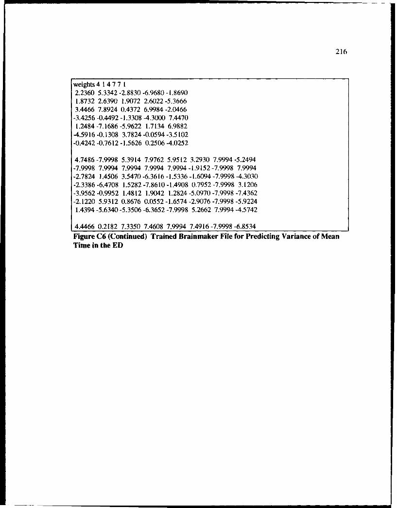
216
weights 4 1 4 7 7 12.2360 5.3342 -2.8830 -6.9680 -1.86901.8732 2.6390 1.9072 2.6022-5.36663.4466 7.8924 0.4372 6.9984 -2.0466
-3.4256 -0.4492 -1.3308 -4.3000 7.44701.2484 -7.1686 -5.9622 1.7134 6.9882
-4.5916 -0.1308 3.7824 -0.0594 -3.5102-0.4242 -0.7612 -1.5626 0.2506 -4.0252
4.7486 -7.9998 5.3914 7.9762 5.9512 3.2930 7.9994 -5.2494-7.9998 7.9994 7.9994 7.9994 7.9994 -1.9152 -7.9998 7.9994-2.7824 1.4506 3.5470 -6.3616 -1.5336 -1.6094 -7.9998 -4.3030-2.3386 -6.4708 1.5282 -7.8610 -1.4908 0.7952 -7.9998 3.1206-3.9562 -0.9952 1.4812 1.9042 1.2824-5.0970 -7.9998 -7.4362-2.1220 5.9312 0.8676 0.0552 -1.6574 -2.9076 -7.9998 -5.92241.4394 -5.6340 -5.3506 -6.3652 -7.9998 5.2662 7.9994 -4.5742
4.4466 0.2182 7.3350 7.4608 7.9994 7.4916 -7.9998 -6.8534Figure C6 (Continued) Trained Brainmaker File for Predicting Variance of MeanTime in the ED
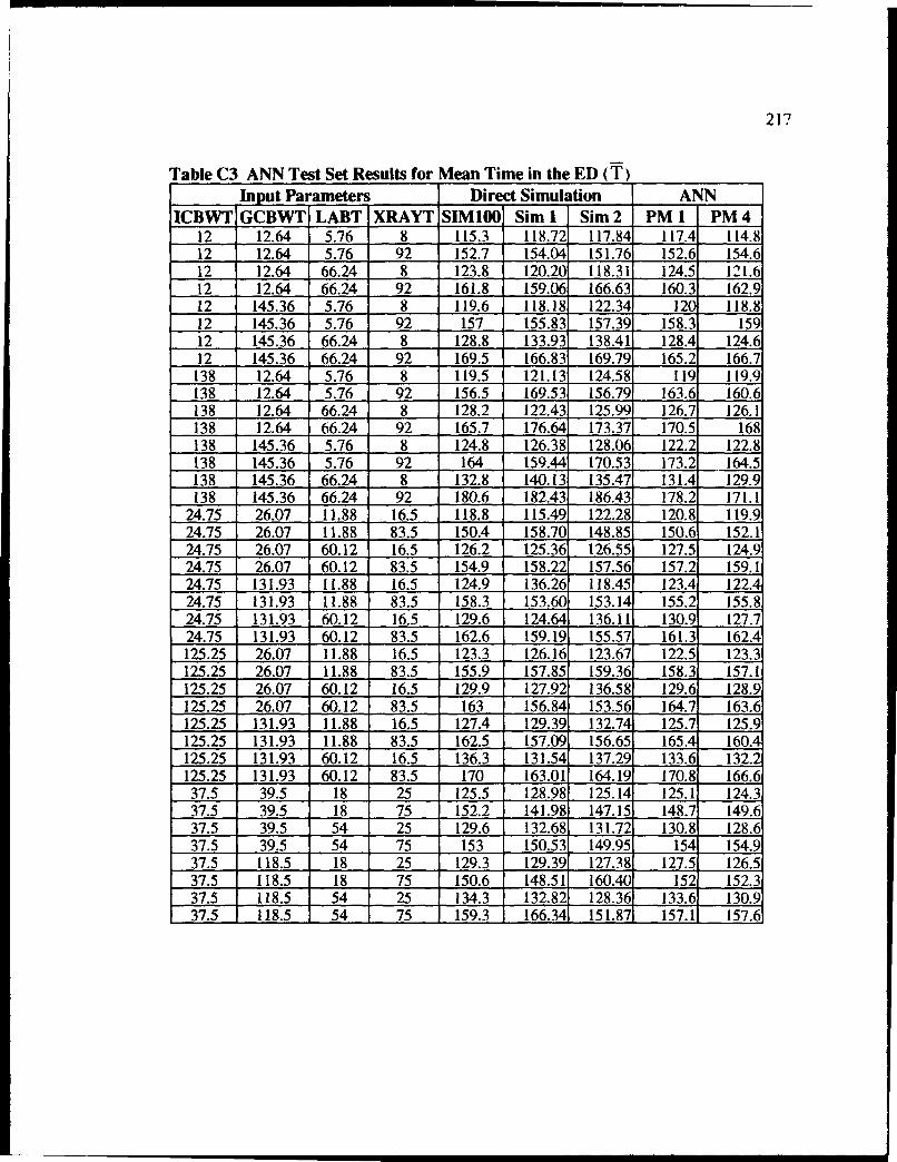
217
Table C3 ANN Test Set Results for Mean Time in the ED (T)Input Parameters Direct Simulation ANN
ICBWT GCBWT LABT XRAYT SIM100 Sim 1 Sim 2 PM 1 PM 412 12.64 5.76 8 115.3 118.72 117.84 117.4 114.812 12.64 5.76 92 152.7 154.04 151.76 152.6 154.612 12.64 66.24 8 123.8 120.20 118.31 124.5 121.612 12.64 66.24 92 161.8 159.06 166.63 160.3 162.912 145.36 5.76 8 119.6 118.18 122.34 120 118.812 145.36 5.76 92 157 155.83 157.39 158.3 15912 145.36 66.24 8 128.8 133.93 138.41 128.4 124.612 145.36 66.24 92 169.5 166.83 169.79 165.2 166.7
138 12.64 5.76 8 119.5 121.13 124.58 119 119.9138 12.64 5.76 92 156.5 169.53 156.79 163.6 160.6138 12.64 66.24 8 128.2 122.43 125.99 126.7 126.1138 12.64 66.24 92 165.7 176.64 173.37 170.5 168138 145.36 5.76 8 124.8 126.38 128.06 122.2 122.8138 145.36 5.76 92 164 159.44 170.53 173.2 164.5138 145.36 66.24 8 132.8 140.13 135.47 131.4 129.9138 145.36 66.24 92 180.6 182.43 186.43 178.2 171.1
24.75 26.07 11.88 16.5 118.8 115.49 122.28 120.8 119.924.75 26.07 11.88 83.5 150.4 158.70 148.85 150.6 152.124.75 26.07 60.12 16.5 126.2 125.36 126.55 127.5 124.924.75 26.07 60.12 83.5 154.9 158.22 157.56 157.2 159.124.75 131.93 11.88 16.5 124.9 136.26 118.45 123.4 122.424.75 131.93 11.88 83.5 158.3 153.60 153.14 155.2 155.824.75 131.93 60.12 16.5 129.6 124.64 136.11 130.9 127.724.75 131.93 60.12 83.5 162.6 159.19 155.57 161.3 162.4125.25 26.07 11.88 16.5 123.3 126.16 123.67 122.5 123.3125.25 26.07 11.88 83.5 155.9 157.85 159.36 158.3 157.1125.25 26.07 60.12 16.5 129.9 127.92 136.58 129.6 128.9125.25 26.07 60.12 83.5 163 156.84 153.56 164.7 163.6125.25 131.93 11.88 16.5 127.4 129.39 132.74 125.7 125.9125.25 131.93 11.88 83.5 162.5 157.09 156.65 165.4 160.4125.25 131.93 60.12 16.5 136.3 131.54 137.29 133.6 132.2125.25 131.93 60.12 83.5 170 163.01 164.19 170.8 166.637.5 39.5 18 25 125.5 128.98 125.14 125.1 124.337.5 39.5 18 75 152.2 141.98 147.15 148.7 149.637.5 39.5 54 25 129.6 132.68 131.72 130.8 128.637.5 39.5 54 75 153 150.53 149.95 154 154.937.5 118.5 18 25 129.3 129.39 127.38 127.5 126.537.5 118.5 18 75 150.6 148.51 160.40 152 152.337.5 118.5 54 25 134.3 132.82 128.36 133.6 130.937.5 118.5 54 75 159.3 166.34 151.87 157.1 157.6
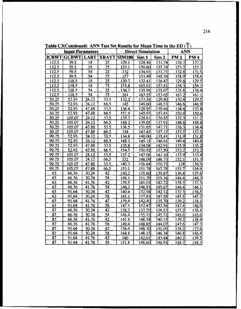
218
Table C3(Continued) ANN Test Set Results for Mean Time in the ED (T)Input Parameters Direct Simulation ANN
ICBWT GCBWT LABT XRAYT SIM100 Sim 1 Sim 2 PM I PM 4112.5 39.5 18 25 129.1 128.46 131.74 126.7 127.2112.5 39.5 18 75 150.1 150.60 155.34 153.7 153.3112.5 39.5 54 25 132 134.01 131.71 132.8 131.9112.5 39.5 54 75 157 151.49 148.36 158.9 158.6112.5 118.5 18 25 130.7 132.41 136.47 129.6 129.5112.5 118.5 18 75 155.8 165.01 153.81 158.3 156.1112.5 118.5 54 25 136.7 135.96 135.07 135.8 134.4112.5 118.5 54 75 161 163.55 153.65 163.2 161.150.25 52.93 24.12 33.5 132.2 133.54 129.80 130.4 129.550.25 52.93 24.12 66.5 145 149.60 148.53 146.6 146.950.25 52.93 47.88 33.5 136.4 128.95 139.64 134.4 132.850.25 52.93 47.88 66.5 151.9 145.93 157.41 150.4 150.650.25 105.07 24.12 33.5 135.2 128.61 136.85 132.3 131.250.25 105.07 24.12 66.5 148.2 139.05 137.91 148.8 148.850.25 105.07 47.88 33.5 136.5 131.65 147.71 136.3 134.450.25 105.07 47.88 66.5 154 147.45 157.15 152.5 152.599.75 52.93 24.12 33.5 134.8 140.00 135.41 131.9 131.899.75 52.93 24.12 66.5 148.2 145.18 146.61 149.4 149.699.75 52.93 47.88 33.5 135.8 134.08 142.91 135.9 135.299.75 52.93 47.88 66.5 154.5 150.92 157.50 153.2 153.299.75 105.07 24.12 33.5 135.2 147.06 141.10 133.9 133.499.75 105.07 24.12 66.5 152 148.09 146.73 152.1 151.399.75 105.07 47.88 33.5 140.3 136.64 150.72 138 136.999.75 105.07 47.88 66.5 153.1 151.78 162.78 155.7 154.9
63 66.36 30.24 42 140.2 135.60 139.67 136.4 135.663 66.36 30.24 58 148.1 151.29 159.34 144.4 144.363 66.36 41.76 42 139.5 141.03 142.72 138.3 137.363 66.36 41.76 58 146.2 148.93 145.67 146.4 146.163 91.64 30.24 42 140.4 132.58 142.12 137.3 136.563 91.64 30.24 58 145.1 137.93 147.58 145.5 145.263 91.64 41.76 42 139.4 142.40 135.70 139.2 138.163 91.64 41.76 58 147.1 152.47 142.56 147.4 146.987 66.36 30.24 42 138.7 137.70 138.53 137.2 136.887 66.36 30.24 58 146.4 155.15 145.32 145.6 145.687 66.36 41.76 42 141.8 148.54 140.33 139.2 138.487 66.36 41.76 58 149.4 148.85 144.07 147.6 147.387 91.64 30.24 42 136.6 148.30 130.09 138.2 137.687 91.64 30.24 58 144.8 148.13 146.34 146.8 146.487 91.64 41.76 42 140 142.01 143.44 140.2 139.587 91.64 41.76 58 151.8 148.60 146.93 148.7 148.3
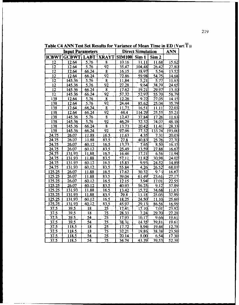
219
Table C4 ANN Test Set Results for Variance of Mean Time in ED (Var(T))Input Parameters Direct Simulation ANN
ICBWT GCBWT LABT XRAYT SIM100 Sim I Sim 212 12.64 5.76 8 10.16 11.11 11.68 15.6212 12.64 5.76 92 35.47 104.48 26.42 27.8012 12.64 66.24 8 16.15 18.97 5.54 13.5212 12.64 66.24 92 72.86 59.98 54.75 14.6812 145.36 5.76 8 11.84 5.21 5.77 11.6312 145.36 5.76 92 27.28 9.64 38.79 24.6512 145.36 66.24 8 17.62 19.21 29.97 13.1012 145.36 66.24 92 57.32 52.97 55.70 58.79138 12.64 5.76 8 12.26 9.22 27.05 14.15138 12.64 5.76 92 24.44 85.62 25.04 35.79138 12.64 66.24 8 11.73 16.51 11.11 22.03138 12.64 66.24 92 44.4 114.29 25.55 55.21138 145.36 5.76 8 12.47 37.84 17.26 11.63138 145.36 5.76 92 46.29 32.32 74.07 48.18138 145.36 66.24 8 13.73 20.42 11.41 28.33138 145.36 66.24 92 97.96 77.32 133.74 193.00
24.75 26.07 11.88 16.5 11.63 4.35 7.31 20.0324.75 26.07 11.88 83.5 27.8 40.83 25.76 27.7024.75 26.07 60.12 16.5 13.73 7.65 8.50 16.1524.75 26.07 60.12 83.5 25.49 13.59 27.88 16.6724.75 131.93 11.88 16.5 16.46 17.21 6.56 11.9424.75 131.93 11.88 83.5 57.11 11.82 30.98 24.0224.75 131.93 60.12 16.5 15.83 9.93 24.52 14.8924.75 131.93 60.12 83.5 55.84 4.26 26.52 68.03125.25 26.07 11.88 16.5 17.62 30.32 9.7,2 16.67125.25 26.07 11.88 83.5 39.04 61.49 23.61 27.17125.25 26.07 60.12 16.5 12.15 3.94 17.01 22.55125.25 26.07 60.12 83.5 40.93 56.25 9.12 37.89125.25 131.93 11.88 16.5 13.42 15.72 34.68 11.63125.25 131.93 11.88 83.5 29.8 11.18 25.05 37.99125.25 131.93 60.12 16.5 18.25 24.50 11.10 25.60125.25 131.93 60.12 83.5 45.97 29.13 86.56 16.9937.5 39.5 18 25 17.41 17.10 7.01 23.9237.5 39.5 18 75 28.33 7.24 29.70 27.2837.5 39.5 54 25 17.93 10.17 9.66 19.6137.5 39.5 54 75 38.31 14.35 39.81 19.6137.5 118.5 18 25 17.72 8.94 19.44 12.7837.5 118.5 18 75 32.21 19.86 38.38 23.5037.5 118.5 54 25 20.14 8.00 6.54 17.3037.5 118.5 54 75 34.74 43.39 39.53 52.38
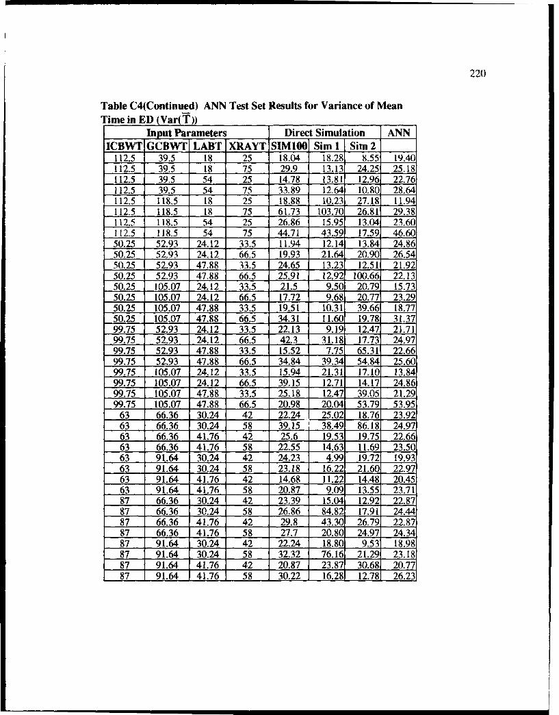
220
Table C4(Continued) ANN Test Set Results for Variance of MeanTime in ED (Var(T))
Input Parameters Direct Simulation ANNICBWT GCBWT LABT XRAYT SIM100 Sim 1 Sim 2
112.5 39.5 18 25 18.04 18.28 8.55 19.40112.5 39.5 18 75 29.9 13.13 24.25 25.18112.5 39.5 54 25 14.78 13.81 12.96 22.76112.5 39.5 54 75 33.89 12.64 10.80 28.64112.5 118.5 18 25 18.88 10.23 27.18 11.94112.5 118.5 18 75 61.73 103.70 26.81 29.38112.5 118.5 54 25 26.86 15.95 13.04 23.60112.5 118.5 54 75 44.71 43.59 17.59 46.6050.25 52.93 24.12 33.5 11.94 12.14 13.84 24.8650.25 52.93 24.12 66.5 19.93 21.64 20.90 26.5450.25 52.93 47.88 33.5 24.65 13.23 12.51 21.9250.25 52.93 47.88 66.5 25.91 12.92 100.66 22.1350.25 105.07 24.12 33.5 21.5 9.50 20.79 15.7350.25 105.07 24.12 66.5 17.72 9.68 20.77 23.2950.25 105.07 47.88 33.5 19.51 10.31 39.66 18.7750.25 105.07 47.88 66.5 34.31 11.60 19.78 31.3799.75 52.93 24.12 33.5 22.13 9.19 12.47 21.7199.75 52.93 24.12 66.5 42.3 31.18 17.73 24.9799.75 52.93 47.88 33.5 15.52 7.75 65.31 22.6699.75 52.93 47.88 66.5 34.84 39.34 54.84 25.6099.75 105.07 24.12 33.5 15.94 21.31 17.10 13.8499.75 105.07 24.12 66.5 39.15 12.71 14.17 24.8699.75 105.07 47.88 33.5 25.18 12.47 39.05 21.2999.75 105.07 47.88 66.5 20.98 20.04 53.79 53.95
63 66.36 30.24 42 22.24 25.02 18.76 23.9263 66.36 30.24 58 39.15 38.49 86.18 24.9763 66.36 41.76 42 25.6 19.53 19.75 22.6663 66.36 41.76 58 22.55 14.63 11.69 23.5063 91.64 30.24 42 24.23 4.99 19.72 19.9363 91.64 30.24 58 23.18 16.22 21.60 22.9763 91.64 41.76 42 14.68 11.22 14.48 20.4563 91.64 41.76 58 20.87 9.09 13.55 23.7187 66.36 30.24 42 23.39 15.04 12.92 22.8787 66.36 30.24 58 26.86 84.82 17.91 24.4487 66.36 41.76 42 29.8 43.30 26.79 22.8787 66.36 41.76 58 27.7 20.80 24.97 24.3487 91.64 30.24 42 22.24 18.80 9.53 18.9887 91.64 30.24 58 32.32 76.16 21.29 23.1887 91.64 41.76 42 20.87 23.87 30.68 20.7787 91.64 41.76 58 30.22 16.28 12.78 26.23

BIBLIOGRAPHY

222
BIBLIOGRAPHY
1 Law, A. and Kelton, W.. Simulation Modeling and Analysis (2nd edition; NewYork: McGraw-Hill, 1991), p. 679
2 Box, G. and Draper, N., Empirical Model Building and Response Surfaces (NewYork: John Wiley & Sons, 1987), pp. 10-1 1.
3 Proceedings of the 1992 Winter Simulation Conference, Arlington, Virginia,December 13-16. 1992, "Metamodels for Simulation Input-Output Relations, by R.Barton" (Piscataway, New Jersey: IEEE, 1992), pp. 289-299.
4 White, H., "Learning in Artificial Neural Networks: A Statistical Perspective,"Neural Computation, Vol. 1 (1989), pp. 425-464.
5 Salvendy, G., ed., Handbook of Industrial Engineering, "Modeling for SimulationAnalysis by A. Pritsker," (New York: John Wiley & Sons, Inc., 1992), pp.2536-2547.
6 Law and Kelton, Op. Cit., p. 115.
7 Oswalt, I., "Current Applications, Trends, and Organizations in the US MilitarySimulation and Gaming," Simulation and Gaming, Vol. 24, No. 2, (1993), pp. 153-189.
8 Law and Kelton, Op. Cit., pp. 114-116.
9 Hillier, F. and Lieberman, G.. Introduction to Operations Research (New York:McGraw-Hill, 1986), p. 826.
10 Jacobson, S. and Schruben. L.. "Techniques for Simulation Response Optimization,"Operations Research Letters, Vol. 8 (Feb 1989), pp. 1-9.
11 Box and Draper, Op. Cit., pp. 17-18.
12 Donohue, J., "The Use of Correlated Simulation Experiments in Response SurfaceOptimization" (unpublished Ph.D. Dissertation, Management Science Department.Virginia Polytechnic Institute and State University, 1988).
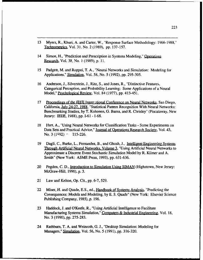
223
13 Myers, R., Khuri, A. and Carter, W., "Response Surface Methodology: 1966-1988,"Technometrics, Vol. 31, No. 2 (1989), pp. 137-157.
14 Simon, H., "Prediction and Prescription in Systems Modeling," OperationsResearch, Vol. 38, No. 1 (1989), p. 11.
15 Padgett, M. and Roppel, T. A., "Neural Networks and Simulation: Modeling forApplications," Simulation, Vol. 58, No. 5 (1992), pp. 295-305.
16 Anderson, J., Silverstein, J., Ritz, S., and Jones, R., "Distinctive Features,Categorical Perception, and Probability Learning: Some Applications of a NeuralModel," Psychological Review, Vol. 84 (1977), pp. 413-451.
17 Proceedings of the IEEE Interr ational Conference on Neural Networks, San Diego,California, July 24-27. 1988, "Statistical Pattern Recognition With Neural Networks:Benchmarking Studies, by T. Kohonen, G. Barna, and R. Chrisley" (Piscataway, NewJersey: IEEE, 1988), pp. 1-61 - 1-68.
18 Hart, A., "Using Neural Networks for Classification Tasks - Some Experiments onData Sets and Practical Advice," Journal of Operations Research Sogimey, Vol. 43,No. 3 (1992)-- 215-226.
19 Dagli, C., Burke, L., Fernandez, B., and Ghosh, J., Intelligent Engineering SystemsThrough Artificial Neural Networks. Volume 3, "Using Artificial Neural Networks toApproximate a Discrete Event Stochastic Simulation Model by R. Kilmer and A.Smith" (New York: ASME Press, 1993), pp. 631-636.
20 Pegden, C. D., Introduction to Simulation Using SIMAN (Highstown, New Jersey:McGraw-Hill, 1990), p. 3.
21 Law and Kelton, Op. Cit., pp. 6-7, 529.
22 Miser, H. and Quade, E.S., ed., Handbook of Systems Analysis, "Predicting theConsequences: Models and Modeling, by E. S. Quade" (New York: Elsevier SciencePublishing Company, 1985), p. 196.
23 Haddock, J. and O'Keefe, R., "Using Artificial Intelligence to FacilitateManufacturing Systems Simulation," Computers & Industrial Engineering, Vol. 18,No. 3 (1990), pp. 275-283.
24 Rathburn, T. A. and Weinroth, G. J., "Desktop Simulation: Modeling forManagers," Simulation, Vol. 56, No. 5 (1991), pp. 316-320.
224
25 Proceedings of the 1993 Winter Simulation Conference, Los Angeles, California,December 12-15. 1993,"Simulation for Real-Time Decision Making in ManufacturingSystems, by P. Rogers and R. Gordon" (Piscataway, New Jersey: IEEE, 1993), pp.866-874.
26 Proceedings of the 1993 Winter Simulation Conference, Los Angeles, California,December 12-15. 1993, "Exception Management on a Shop Floor Using OnlineSimulation, by D. Katz and S. Manivannan" (Piscataway, New Jersey: IEEE, 1993),pp. 888-896.
27 Proceedings of the 1993 Winter Simulation Conference, Los Angeles, California,December 12-15. 1993, "Domain-Based On-Line Simulation for Real-Time DecisionSupport, by M. Krishnamurthi and S. Vasudevan" (Piscataway, New Jersey: IEEE,1993), pp. 1304-1312.
28 Mann, W. and Loerch, A., Response Surface Methodology for Value AddedAnalysis, ARO Report 92-2 (Washington, D.C.: Army Research Office, 1992), pp.285-296.
29 Kleijnen, J., van Ham, G., Rotmans, J., "Techniques for Sensitivity Analysis ofSimulation Models: A Case Study of the C02 Greenhouse Effect," Simulation, Vol.58, No. 6 (1992), pp. 410-417.
30 Pratt, David, B., "Development of a Methodology for Hybrid Metamodeling ofHierarchical Manufacturing Systems within a Simulation Framework" (unpublishedPh.D. Dissertation, School of Industrial Engineering and Management, OklahomaState University, 1992).
31 Proceedings of the 1972 Summer Simulation Conference, San Diego, California,June 14-16. 1972, "Techniques for the Development of Empirical Subsystem Models,by M. Racite and F. Lawlor" (La Jolla, California: Simulation Councils, Inc., 1972),pp. 155-162.
32 Safizadeh, M. H., "Optimization in Simulation: Current Issues and the FutureOutlook," Naval Research Logistics, Vol. 37, (1990), pp. 807-825.
33 Lippmann, Richard, D., "An Introduction to Computing with Neural Nets", IEEEAS ,Lagzinm, Vol. 4, No. 4, (1987), pp. 4-22.
34 Graubard, Stephan R., ed., The Artificial Intelligence Debate-False Starts. RealFoundations, "Neural Nets and Artificial Intelligence, by J. D. Cowan, and D. H.Sharp" (Cambridge, Massachusetts: The MIT Press, 1988), pp. 85-121.
225
35 Hertz, J., Krogh, A. and Palmer, R., Introduction to the Theory of NeuralComputation (Redwood City, California: Addison-Wesley, 199 1), pp. 6-8.
36 Zurada, J., Introduction to Artificial Neural Systems (New York: West PublishingCompany, 1992), pp. 17-22, 455-664.
37 Cheng, B. and Titterington, D., "Neural Networks: A Review from a StatisticalPerspective," Statistical Science, Vol. 9, No. 1 (1994), pp. 2-54.
38 Feldman, J., Hayes, P., and Rumelhart, D., ed., Parallel Distributed ProcessingExplorations in the Microstructure of Cognition Volume 1: Foundations, "P3 AParallel Network Simulating System, by D. Zipser and D. E. Rabin" (Cambridge,Massachusetts: The MIT Press, 1986), pp. 488-501.
39 Muller, B. and Reinhardt, J., Neural Networks: An Introduction (Berlin: Springer-Verlag, 1990), pp. 62-70.
40 Nelson, M. and Illingworth, W., A Practical Guide to Neural Nets, (Reading,
Massachusetts: Addison-Wesley, 1991), p. 46.
41 Zurada, Op. Cit., p. 182.
42 Melsa, P., Neural Networks: A Conceptual Overview, Technical Report 89-08(Mishawaka, Indiana: Tellabs Research Center, Aug, 1989).
43 S. Brahim, A. Smith, and B. Bidanda, "Relating Product Specifications andPerformance Data with a Neural Network Model for Design Improvement", Journalof Intelligent Manufacturing, Vol 4, (1993), pp. 367-374.
44 Werbos, P., "Beyond Regression: New Tools for Prediction and Analysis in theBehavioral Sciences," (unpublished Ph.D. dissertation, Harvard University,Department of Applied Mathematics, 1974) reprinted in P. Werbos, The Root ofBackpropagation: From Ordered Derivatives to Neural Networks to PoliticalForcastirng (New York: John Wiley & Sons, 1993).
45 Feldman, J., Hayes, P., and Rumelhart, D., ed., Parallel Distributed ProcessingExplorations and the Microstructure of Cognition Volume 1: Foundations, "LearningInternal Representations by Error Propagation, by D. E. Rumelhart, G. E. Hinton, andR. J. Williams" (Cambridge, Massachusetts: The MIT Press, 1986), pp. 318-362.
46 Kreinovich, V. Y., "Arbitrary Nonlinearity Is Sufficient to Represent Functions byNeural Networks: A Theorem," Neulr Networks, Vol. 4 (1991), pp. 381-383.

226
47 Cybenko, G., "Approximation by Superpositions of a Sigmoidal Function,"Mathematical Control Signals Systems, Vol. 2 (1989), pp. 303-31.
48 Hornik, K., Stinchcombe, M. and White, H., "Multilaver Feedforward Networks aweUniversal Approximators," Neural Networks, Vol. 2 (1989), pp. 359-366.
49 Wang, W., "A Nonlinear Function Approximator - The Cooperation ofNonparametric Concepts and a Neural Network Approach" (unpublished Ph.D.Dissertation, School of Industrial and Systems Engineering, Ohio State University,1989).
50 Hornik, K., Stinchcombe, M. and White, H., "Universal Approximation of anUnknown Mapping and Its Derivatives Using Multilayer Feedforward Networks,"Neural Networks, Vol. 3 (1990), pp. 551-560.
51 Poggio, T. and Girosi, F., A Theory of Networks for Approximation and Learning,Artificial Intelligence Memorandum No. 1140. C.B.I.P. Paper No. 31 (Cambridge,Massachusetts: MIT, 1989).
52 Girosi, F., Poggio, T., and Caprile, B., Extensions of A Theory of Networks forApproximation and Learning, Artificial Intelligence Memorandum No 1220, C.B.I.P.Paper No. 46 (Cambridge, Massachusetts: MIT, 1990).
53 Homik, K., "Approximation Capabilities of Multilayer Feedforward Networks,"Neural Networks, Vol. 4 (1991), pp. 251-257.
54 Cardaliguet, P. and Euvrard, G., "Approximation of a Function and its Derivativewith a Neural Network," Neural Networks, Vol. 5 (1992), pp. 207-220.
55 Haykin, Op. Cit., pp. 190-191.
56 Gon, M. and Tesi, A., "On the Problem of Local Minima in Backpropagation,"IEEE Transactions on Pattern Analysis and Machine Intelligence, Vol. 14, No. 1(1992), pp. 76-86.
57 Hush, D. and Home, B., "Progress in Supervised Neural Networks: What's NewSince Lippmann?," IEEE Signal Processing Magazine, Vol. 10, No. 1 (1993), pp. 8-39.
58 Proceedings of the 1988 Connectionist Models Summer School, Pittsburgh,Pennsylvania, "Faster-Learning Variations on Back-Propagation: An Emperical Studyby S. Fahlman" (San Mateo, California: Kaufman, 1989), pp. 38-51.
227
59 Proceedings of the IEEE International Conference on Neural Networks 1993, SanFrancisco, California, March 28-April 1. 1993, "A Direct Adaptive Method for FasterBackpropagation Learning: The RPROP Algorithm, by M. Reidmiller and H. Braun"(Piscataway, New Jersey: IEEE, 1993), pp. 586-591.
60 Drucker, H. and Cun, Y., "Improving Generalizing Performance Using DoubleBackpropagation," IEEE Transactions on Neural Networks, Vol.3, No. 6 (1992), pp.991-997.
61 Proceedings of the 1988 Connectionist Models Summer School, Pittsburgh,Pennsylvania, "Improving the Convergence of Backpropagation Learning withSecond Order Methods by S. Becker and Y. Cun" (San Mateo, California: Kaufman,1989), pp. 29-37.
62 Piramuthu, S., Kuan, C., Shaw, M., "Learning Algorithms for Neural-Net DecisionSupport," ORSA Journal on Computing, Vol. 5, No. 4 (1993), pp. 361-373.
63 Proceedings of the IEEE International Conference on Neural Networks 1993, SanFrancisco, California, March 28-April 1. 1993, "Supervised Learning for Feed-Forward Neural Networks: A New Minimax Approach for Fast Convergence, by A.Chella, A. Gentile, F. Sorbello, and A. Tarantino" (Piscataway, New Jersey: IEEE,1993), pp. 605-609.
64 Van der Smagt, P., "Minimization Methods for Training Feed Forward NeuralNetworks," Neural Networks, Vol. 7, No. 1 (1994), pp. 1-11.
65 Proceedings of the World Congress of Neural Networks. Volume 3, Portland,Oregon, July 11-15. 1993, "Supervised Learning: Can It Escape Its Local Minimum?,by P. Werbos" (Hillsdale, New Jersey: Lawrence Erlbaum Associates, Inc., 1993),pp. 358-363.
66 Girosi, F. and Poggio, T., "Networks and the Best Approximation Property,"Biological Cybernetics, Vol. 63 (1990), pp. 169-176.
67 Leonard, J., Kramer, M., Ungar, L., "Using Radial Basis Functions to Approximatea Function and Its Error Bounds," IEEE Transactions on Neural Networks, Vol. 3,No. 4 (1992), pp. 624-627.
68 Funahashi, K. "On the Approximate Realization of Continuous Mappings by NeuralNetworks," Neural Ntworks, Vol. 2 (1989), pp. 183-192.
228
69 Chen, T. and Chen, H., "Approximations of Continuous Functionals by NeuralNetworks with Application to Dynamic Systems," IEEE Transactions on NeuralNetworks, Vol. 4, No. 6 (1993), pp. 910-918.
70 Proceedings of the International Joint Conference on Neural Networks, San Diego,California, June 17-21. 1990, "Why Two Hidden Layers Are Better Than One, by D.Chester" (Piscataway, New Jersey: IEEE, 1990), pp. 1-265 - 1-268.
71 Anderson, D., ed., Neural Information Processing Systems, "How Neural NetsWork by A. Lapedes and R. Farber" (New York: American Institute of Physics,1988), pp. 442-456.
72 Proceedings of the 1992 Summer Computer Simulation Conference, Reno, Nevada,July 27-30. 1992, "Design of a Neural Network Module for Integration into aSimulation, by M. Padgett and T. Roppel" (San Diego, California: Society forComputer Simulation, 1992), pp. 390-395.
73 Proceedings of the 1989 Winter Simulation Conference, Washington, D. C.,December 4-6. 1989, "Neural Network Models in Simulation: A Comparison withTraditional Modeling Approaches, by P. Fishwick" (Piscataway, New Jersey: IEEE,1989), pp. 702-710.
74 Proceedings of the 1992 Summer Computer Simulation Conference, Reno, Nevada,July 27-30. 1992, "An Investigation on Neural Network Capabilities as SimulationMetamodels, by H. Pierreval and R. Huntsinger" (San Diego, California: Society forComputer Simulation, 1992), pp. 413-417.
75 Badiru, A. and Sieger, D., Neural Network as a Simulation Metamodel in EconomicAnalysis of Risky Projects (Norman, Oklahoma: Department of IndustrialEngineering, University of Oklahoma, 1993).
76 Hurrion, R. D., "Using a Neural Network to Enhance the Decision Making Qualityof a Visual Interactive Simulation Model," Journal of the Operations ResearchS..i.l,, Vol. 43, No. 4 (1992), pp. 333-341.
77 Hurrion, R. D. and Secker, R. J. R., "Visual Interactive Simulation An Aid toDecision Making," The International Journal of Management Science, Vol. 6, No. 5(1978), pp. 419-426.
78 Hurrion, Op. Cit., p.338.
229
79 Hoskins, D. A., Hwang, J. N., Vagners, J., "Iterative Inversion of Neural Networksand Its Application to Adaptive Control," IEEE Transactions on Neural Networks,Vol. 3, No. 2 (1992), pp. 292-301.
80 Kil, R., "Approximation and Inverse Mapping of Continuous Functions in theParadigms of Connectionist Models: Theories and Applications" (unpublished Ph.D.Dissertation, School of Computer Engineering, University of Southern California,1991).
81 Miller, W., Sutton, R., Werbos, P., ed., Neural Networks for Control,"Connectionist Learning for Control by A. Barto" (Cambridge, Massachusetts: TheMIT Press, 1990), pp. 5-58.
82 Chyssolouris, G., Lee, M., Pierce, J., and Domroese, M., "Use of Neural Networksfor the Design of Manufacturing Systems," Manufacturing Review, Vol. 3, No. 3(1989), pp. 198-194.
83 Morrison, J.D., "A'Neural' Network Model that Supports Realtime Learning ofTemporal Relationships in Complex Engineering Domains," Simulation, Vol. 59, No.3 (1992), pp. 152-163.
84 Ibid., p. 162.
85 Miller, W., Sutton, R., Werbos, P., eds., Neural Networks for Control. "Overviewof Designs and Capabilities, by P. Werbos" (Cambridge, Massachusetts: The MITPress, 1990), pp. 59-66.
86 Smith, A. and Dagli, C., "Controlling Industrial Processes Through Supervised,Feedforward Neural Networks," Computers & Industrial Engineering, Vol. 21, No. 1-4, (1991), pp. 247-251.
87 Proceedings of the 1992 Summer Computer Simulation Conference, Reno, Nevada,July 27-30. 1992, "Neural Networks for Defense- A Control System Application, byM. Padgett, T. Roppel, and U. Desai" (San Diego, California: Society for ComputerSimulation, 1992), pp. 396-402.
88 Proceedings of the IEEE International Conference on Neural Networks, SanFrancisco, California, March 28-April 1. 1993, "Intelligent FMS Scheduling UsingModular Neural Networks, by L. Rabelo, Y. Yih, A. Jones, and G. Witzgall"(Piscataway, New Jersey: IEEE, 1993), pp. 1224-1229.
230
89 Proceedings of the 3rd Workshop on Neural Networks: Academic/Industrial/NASA/Defense. SPIE Volume 1721, Auburn University, Alabama, February 10-12.12M, "A Manufacturing Cell Control Strategy Using Discrete Event Simulation, byQ. Wan, and J. Cochran" (San Diego, California: Society for Computer Simulation,1992), pp. 217-222.
90 Kleijnen, J., "Regression Metamodels for Generalizing Simulation Results," IEEETransactions on Systems. Man. and Cybernetics, Vol. 9, No. 2 (1979), pp. 93-96.
91 Blanning, R., "The Sources and Uses of Sensitivity Information," Interfaces, Vol. 4,No. 4 (1974), pp. 32- 38.
92 Blanning, R., "The Construction and Implementation of Metamodels," Simulation,Vol. 24, (1975), pp. 177-184.
93 Meisel, W. and Collins, D., "Repro-Modeling: An Approach to Efficient ModelUtilization and Interpretation," IEEE Transactions on Systems. Man and Cybernetics,Vol. 3, No. 4 (1973), pp. 349-358.
94 Friedman, L. and Pressman, I., "The Metamodel in Simulation Analysis: Can It BeTrusted?," Journal of the Operations Research Society, Vol. 39, No. 10 (1988), pp.939-948.
95 Pratt, D. and Mize, J., A Methodology for Simulation Metamodeling ofManufacturing Systems, CIM-TRS-93-DP1 (Stillwater, Oklahoma: Center forComputer Integrated Manufacturing, Oklahoma State University, 1993).
96 Yu, B. and Popplewell, K., "Metamodels in Manufacturing: A Review,"International Journal of Production Research, Vol. 32 (1994), pp. 787-796.
97 Rotmans, J. and Vrieze, 0., "Metamodeling and Experimental Design: Case Studyof the Greenhouse Effect," European Journal of Operations Research, Vol. 47,(1990), p. 321.
98 Montgomery, D. and Bettencourt, V., "Multiple Response Surface Methods inComputer Simulation," Simulation, Vol. 29 (1977), pp. 113-121.
99 Gardenier, T. K., "Pre-Prim as a Pre-Processor to Simulations: a Cohesive Unit,"S, Vol. 24, No 2 (1990), pp. 65-70.
100 Draper, N. and Smith, H., Applied Regression Analysis (2nd edition; New York:John Wiley & Sons, 1981), pp. 22-126, 218-221.
231
101 Ibid., pp. 22-23.
102 Ibid., pp. 108-115.
103 Ibid., pp. 237-239.
104 Ibid., pp. 458-529.
105 Khuri, A. and Cornell, J., Response Surfaces Designs and Analyses (New York:Marcel Dekker, Inc., 1987), pp. 303-33 1.
106 Thompson, J. and Tapia, R., Nonparametric Function Estimation. Modeling andSimulation (Philadelphia, Pennsylvania: Society for Industrial and AppliedMathematics, 1990), pp. 186-196.
107 Hardle, W., Applied Nonparametric Regression (Cambridge, UK: CambridgeUniversity Press, 1990)
108 Box, G. and Wilson, K. "On the Experimental Attainment of Optimum Conditions,"Journal of the Royal Statistics Society, Vol. 13, Ser. B, (1951), pp. 1-45.
109 Khuri and Cornell, Op. Cit., pp. 1 - 17.
110 Hussey, J., Myers, R., Houck, E., "Correlated Simulation Experiments in First-Order Response Surface Design," Operations Research, Vol. 35, N( (1987), pp.744-758.
111 Donohue, J., Houck, E., Myers, R., "Simulation Designs for Quadratic ResponseSurface Models in the Presence of Model Misspecification," Management Science,Vol. 38, No. 12 (1992), pp. 1765-1791.
112 Proceedings of the 1993 Winter Simulation Conference, Los Angeles, California,December 12-15. 1993, "Response Surface Methodology and its Application inSimulation, by S. Hood and P. Welch" (Piscataway, New Jersey: IEEE, 1993), pp.115-122.
113 Taguchi, G., "Linear Graphs for Orthogonal Arrays and their Application toExperimental Design, with the Aid of Various Techniques," Reports of StatisticalApplication Research. Union of Japanese Scientists and Engineers, Vol. 6, No. 4(1959), pp. 1-43.
232
114 Taguchi, G., System of Experimental Design: Engineering Methods to OptimizeQuality and Minimize Costs Volume 1 and 2, (Dearborn, Michigan: AmericanSupplier Institute, 1987).
115 Ross, P., Taguchi Techniques for Quality Engineering (New York: McGraw-Hill,1988).
116 Proceedinigs of the 1991 Winter Simulation Conference, Phoenix, Arizona,December 8-11. 1991, "Designing Simulation Experiments: Taguchi Methods andResponse Surface Metamodels, by J. Ramberg, S. Sanchez, P. Sanchez, and L.Hollick" (Piscataway, New Jersey: IEEE, 1991), pp. 167-176.
117 Wild, R. and Pignatiello, J., "An Experimental Design Strategy for Designing RobustSystems Using Discrete-event Simulation," Simulation, Vol. 57, No. 6 (1991), pp.358-368.
118 Mayer, R. and Benjamin, P., "Using the Taguchi Paradigm for ManufacturingSystem Design Using Simulation Experiments," Computers & Industrial Engineering,Vol. 22, No. 2 (1992), pp. 195-209.
119 Kuei, C. and Madu, C., "Polynomial Metamodelling and Taguchi Designs inSimulation with Application to the Maintenance Plant System," European Journal of
_Oerational Research, Vol. 72, (1994), pp. 364-375.
120 Schmidt, S. and Launsby, R., Understanding Industrial Designed Experiments (3rdedition; Colorado Springs, Colorado: Air Academy Press, 1992), pp. 6-1 - 6-21.
121 Poggio, T., and Girosi, F., "Networks for Approximation and Learning,"Proceedings of the IEEE, Vol. 78, No. 9 (1990), pp. 1481-1497.
122 Lorentz, G. G., Approximation of Functions (New York: Chelsea PublishingCompany, 1986).
123 Chen, D., "Function Representation and Approximation by Neural Networks,"(unpublished Ph.D. Dissertation, School of Computer Science and Engineering, TheUniversity of Michigan, 1991).
124 Law and Kehlcn, Op. Cit., pp. 679-689.
125 Khuri and Cornell, Op. Cit., pp. 13-16.
126 Law and Kelton, Op. Cit., pp. 248-249.
233
127 Pegden, Op. Cit., p. 25.
128 Pegden, Op. Cit., p. 62.
129 Brainmaker Professional Neural Network Simulation Software User's Guide andReference Manual (3rd edition; Nevada City, California: California ScientificSoftware, April 1992), pp. 5.16-5.24, 14.12-14.16.
130 Proceedings of the IEEE International Joint Conference on Neural Networks,Washington, D.C., June 18-22. 1989, "Theory of the Backpropagation NeuralNetwork, by Robert Hecht-Nielson" (Piscataway, New Jersey: IEEE, 1989), pp. I-593 - 1-605.
131 Zurada, Op. Cit., pp. 175-213.
132 California Scientific Software, BrainMaker Professional (4th edition; Nevada City,California: California Scientific Software, 1993), pp. 235-242.
133 Haykin, S., Neural Networks A Comprehensive Foundation (New York: MacmillanCollege Publishing Company, 1994), pp. 152, 162.
134 Law and Kelton, Op. Cit., pp. 679-689.
135 Nahmias, S., Production and Operations Analysis (Homewood, Illinois: Irwin,1989), pp. 194-211
136 Zheng, Y. and Federgruen, A., "Finding Optimal (s, S) Policies is About as Simpleas Evaluating a Single Policy," Operations Research, Vol. 39, No. 4 (1991), pp. 654-665.
137 Law and Kelton, Op. Cit., p. 687.
138 Kilmer and Smith, Op. Cit., p. 635.
139 Finnoff, W., Hergert, F., Zimmermann, H., "Improving Model Selection by Non-Convergent Methods," Neural Networks, Vol. 6 (1993), pp. 771-783.
140 Willemain, T. R. and Larsen, R. C., eds., Emergency Medical Systems Analysis,"Using Interactive Graphics in Simulating the Hospital Emergency Department, by R.W. Weissberg" (Lexington, Massachusetts: Lexington Books, 1977), pp. 119-140.
234
141 Saunders, C., Makens, P. and Leblanc, L., "Modeling Emergency DepartmentOperations Using Advanced Computer Simulation Systems," Annals of EmergencyMedicine, Vol. 18 (1989), pp. 134-140.
142 Yu and Popplewell, Op. Cit., pp. 793-794.
143 Proceedings of the World Congress on Neural Networks 1993 Volume 3, Portland,Oregon, July I I-15. 1993, "Learning from What's Been Learned: SupervisedLearning in Multi-Neural Network Systems, by M. Perrone and L. Cooper,"(Hillsdale, New Jersey: Lawrence Erlbaum Associates, Inc., 1993), pp. 354-357.
144 Proceedings of the 1993 Winter Simulation Conference, Los Angeles, California,December 12-15. 1993, "Families of Models that Cross Levels of Resolution: Issuesfor Design, Calibration and Management by P. Davis and R. Hillestad" (Piscataway,New Jersey: IEEE, 1993), pp. 1003-1012.
145 Goldberg, D., Genetic Algorithms in Search. Optimization and Machine Learning(New York: Addison Wesley, 1989), p. 7.


![ACCESSORIES Magnum PRO Semiautomatic Guns · Magnum® PRO Semiautomatic Guns | [ 5 ] EXPENDABLE PARTS Contact Tip for 550A GAS DIFFUSER 550A Type Pkg. Qty. Thread-on Standard Duty](https://img.pdfslide.us/doc/110x75/5e7029bfb168d6338c6dcbfb/accessories-magnum-pro-semiautomatic-guns-magnum-pro-semiautomatic-guns-5.jpg)