Embed Size (px)
Citation preview

2
Probability Theory and Classical Statistics
Statistical inference rests on probability theory, and so an in-depth under-standing of the basics of probability theory is necessary for acquiring a con-ceptual foundation for mathematical statistics. First courses in statistics forsocial scientists, however, often divorce statistics and probability early withthe emphasis placed on basic statistical modeling (e.g., linear regression) inthe absence of a grounding of these models in probability theory and prob-ability distributions. Thus, in the first part of this chapter, I review somebasic concepts and build statistical modeling from probability theory. In thesecond part of the chapter, I review the classical approach to statistics as itis commonly applied in social science research.
2.1 Rules of probability
Defining “probability” is a difficult challenge, and there are several approachesfor doing so. One approach to defining probability concerns itself with thefrequency of events in a long, perhaps infinite, series of trials. From that per-spective, the reason that the probability of achieving a heads on a coin flip is1/2 is that, in an infinite series of trials, we would see heads 50% of the time.This perspective grounds the classical approach to statistical theory and mod-eling. Another perspective on probability defines probability as a subjectiverepresentation of uncertainty about events. When we say that the probabilityof observing heads on a single coin flip is 1/2, we are really making a seriesof assumptions, including that the coin is fair (i.e., heads and tails are infact equally likely), and that in prior experience or learning we recognize thatheads occurs 50% of the time. This latter understanding of probability groundsBayesian statistical thinking. From that view, the language and mathematicsof probability is the natural language for representing uncertainty, and thereare subjective elements that play a role in shaping probabilistic statements.
Although these two approaches to understanding probability lead to dif-ferent approaches to statistics, some fundamental axioms of probability are

10 2 Probability Theory and Classical Statistics
important and agreed upon. We represent the probability that a particularevent, E, will occur as p(E). All possible events that can occur in a single trialor experiment constitute a sample space (S), and the sum of the probabilitiesof all possible events in the sample space is 11:
∑
∀E∈S
p(E) = 1. (2.1)
As an example that highlights this terminology, a single coin flip is atrial/experiment with possible events “Heads” and “Tails,” and therefore hasa sample space of S = {Heads, Tails}. Assuming the coin is fair, the probabil-ities of each event are 1/2, and—as used in social science—the record of theoutcome of the coin-flipping process can be considered a “random variable.”
We can extend the idea of the probability of observing one event in one trial(e.g., one head in one coin toss) to multiple trials and events (e.g., two headsin two coin tosses). The probability assigned to multiple events, say A andB, is called a “joint” probability, and we denote joint probabilities using thedisjunction symbol from set notation (∩) or commas, so that the probabilityof observing events A and B is simply p(A,B). When we are interested in theoccurrence of event A or event B, we use the union symbol (∪), or simply theword “or”: p(A ∪B) ≡ p(A or B).
The “or” in probability is somewhat different than the “or” in commonusage. Typically, in English, when we use the word “or,” we are referringto the occurrence of one or another event, but not both. In the language oflogic and probability, when we say “or” we are referring to the occurrence ofeither event or both events. Using a Venn diagram clarifies this concept (seeFigure 2.1).
In the diagram, the large rectangle denotes the sample space. Circles Aand B denote events A and B, respectively. The overlap region denotes thejoint probability p(A,B). p(Aor B) is the region that is A only, B only, andthe disjunction region. A simple rule follows:
p(A or B) = p(A) + p(B)− p(A,B). (2.2)
p(A,B) is subtracted, because it is added twice when summing p(A) and p(B).There are two important rules for joint probabilities. First:
p(A,B) = p(A)p(B) (2.3)
iff (if and only if) A and B are independent events. In probability theory,independence means that event A has no bearing on the occurrence of eventB. For example, two coin flips are independent events, because the outcomeof the first flip has no bearing on the outcome of the second flip. Second, if Aand B are not independent, then:
1 If the sample space is continuous, then integration, rather than summation, isused. We will discuss this issue in greater depth shortly.

2.1 Rules of probability 11
A B
A∩B
A∪BNot A∪B
Fig. 2.1. Sample Venn diagram: Outer box is sample space; and circles are eventsA and B.
p(A,B) = p(A|B)p(B). (2.4)
Expressed another way:
p(A|B) =p(A,B)
p(B). (2.5)
Here, the “|” represents a conditional and is read as “given.” This last rule canbe seen via Figure 2.1. p(A|B) refers to the region that contains A, given thatwe know B is already true. Knowing that B is true implies a reduction in thetotal sample space from the entire rectangle to the circle B only. Thus, p(A)is reduced to the (A,B) region, given the reduced space B, and p(A|B) is theproportion of the new sample space, B, which includes A. Returning to therule above, which states p(A,B) = p(A)p(B) iff A and B are independent,if A and B are independent, then knowing B is true in that case does notreduce the sample space. In that case, then p(A|B) = p(A), which leaves uswith the first rule.

12 2 Probability Theory and Classical Statistics
Although we have limited our discussion to two events, these rules gener-alize to more than two events. For example, the probability of observing threeindependent events A, B, and C, is p(A,B,C) = p(A)p(B)p(C). More gener-ally, the joint probability of n independent events, E1, E2 . . . En, is
∏ni=1 p(Ei),
where the∏
symbol represents repeated multiplication. This result is veryuseful in statistics in constructing likelihood functions. See DeGroot (1986)for additional generalizations. Surprisingly, with basic generalizations, thesebasic probability rules are all that are needed to develop the most commonprobability models that are used in social science statistics.
2.2 Probability distributions in general
The sample space for a single coin flip is easy to represent using set notationas we did above, because the space consists of only two possible events (headsor tails). Larger sample spaces, like the sample space for 100 coin flips, orthe sample space for drawing a random integer between 1 and 1,000,000,however, are more cumbersome to represent using set notation. Consequently,we often use functions to assign probabilities or relative frequencies to allevents in a sample space, where these functions contain “parameters” thatgovern the shape and scale of the curve defined by the function, as well asexpressions containing the random variable to which the function applies.These functions are called “probability density functions,” if the events arecontinuously distributed, or “probability mass functions,” if the events arediscretely distributed. By continuous, I mean that all values of a randomvariable x are possible in some region (like x = 1.2345); by discrete, I meanthat only some values of x are possible (like all integers between 1 and 10).These functions are called “density” and “mass” functions because they tell uswhere the most (and least) likely events are concentrated in a sample space.We often abbreviate both types of functions using “pdf,” and we denote arandom variable x that has a particular distribution g(.) using the genericnotation: x ∼ g(.), where the “∼” is read “is distributed as,” the g denotes aparticular distribution, and the “.” contains the parameters of the distributiong.
If x ∼ g(.), then the pdf itself is expressed as f(x) = . . . , wherethe “. . .” is the particular algebraic function that returns the relative fre-quency/probability associated with each value of x. For example, one of themost common continuous pdfs in statistics is the normal distribution, whichhas two parameters—a mean (µ) and variance (σ2). If a variable x has prob-abilities/relative frequencies that follow a normal distribution, then we sayx ∼ N(µ, σ2), and the pdf is:
f(x) =1√
2πσ2exp
{
− (x− µ)2
2σ2
}
.
2.2 Probability distributions in general 13
We will discuss this particular distribution in considerable detail through-out the book; the point is that the pdf is simply an algebraic function that,given particular values for the parameters µ and σ2, assigns relative frequen-cies for all events x in the sample space.
I use the term “relative frequencies” rather than “probabilities” in dis-cussing continuous distributions, because in continuous distributions, techni-cally, 0 probability is associated with any particular value of x. An infinitenumber of real numbers exist between any two numbers. Given that we com-monly express the probability for an event E as the number of ways E canbe realized divided by the number of possible equally likely events that canoccur, when the sample space is continuous, the denominator is infinite. Theresult is that the probability for any particular event is 0. Therefore, insteadof discussing the probability of a particular event, we may discuss the proba-bility of observing an event within a specified range. For this reason, we needto define the cumulative distribution function.
Formally, we define a “distribution function” or “cumulative distributionfunction,” often denoted “cdf,” as the sum or integral of a mass or densityfunction from the smallest possible value for x in the sample space to somevalue X, and we represent the cdf using the uppercase letter or symbol thatwe used to represent the corresponding pdf. For example, for a continuous pdff(x), in which x can take all real values (x ∈ R),
p(x < X) = F (x < X) =
∫ X
−∞
f(x) dx. (2.6)
For a discrete distribution, integration is replaced with summation andthe “<” symbol is replaced with “≤,” because some probability is associatedwith every discrete value of x in the sample space.
Virtually any function can be considered a probability density function,so long as the function is real-valued and it integrates (or sums) to 1 overthe sample space (the region of allowable values). The latter requirement isnecessary in order to keep consistent with the rule stated in the previoussection that the sum of all possible events in a sample space equals 1. It isoften the case, however, that a given function will not integrate to 1, hencerequiring the inclusion of a “normalizing constant” to bring the integral to1. For example, the leading term outside the exponential expression in thenormal density function (1/
√2πσ2) is a normalizing constant. A normalized
density—one that integrates to 1—or a density that can integrate to 1 withan appropriate normalizing constant is called a “proper” density function. Incontrast, a density that cannot integrate to 1 (or a finite value), is called “im-proper.” In Bayesian statistics, the propriety of density functions is important,as we will discuss throughout the remainder of the book.
Many of the most useful pdfs in social science statistics appear compli-cated, but as a simple first example, suppose we have some random variablex that can take any value in the interval (a, b) with equal probability. This
14 2 Probability Theory and Classical Statistics
is called a uniform distribution and is commonly denoted as U(a, b), where aand b are the lower and upper bounds of the interval in which x can fall. Ifx ∼ U(a, b), then
f(x) =
{
c if a < x < b0 otherwise.
(2.7)
What is c? c is a constant, which shows that any value in the interval (a, b)is equally likely to occur. In other words, regardless of which value of x onechooses, the height of the curve is the same. The constant must be determinedso that the area under the curve/line is 1. A little calculus shows that thisconstant must be 1/(b− a). That is, if:
∫ b
a
c dx = 1,
thenc x|ba = 1,
and so
c =1
(b− a).
Because the uniform density function does not depend on x, it is a rectangle.Figure 2.2 shows two uniform densities: the U(−1.5, .5) and the U(0, 1) den-sities. Notice that the heights of the two densities differ; they differ becausetheir widths vary, and the total area under the curve must be 1.
The uniform distribution is not explicitly used very often in social scienceresearch, largely because very few phenomena in the social sciences followsuch a distribution. In order for something to follow this distribution, valuesat the extreme ends of the distribution must occur as often as values in thecenter, and such simply is not the case with most social science variables.However, the distribution is important in mathematical statistics generally,and Bayesian statistics more specifically, for a couple of reasons. First, randomsamples from other distributions are generally simulated from draws from uni-form distributions—especially the standard uniform density [U(0, 1)]. Second,uniform distributions are commonly used in Bayesian statistics as priors onparameters when little or no information exists to construct a more informa-tive prior (see subsequent chapters).
More often than not, variables of interest in the social sciences followdistributions that are either peaked in the center and taper at the extremes,or they are peaked at one end of the distribution and taper away from that end(i.e., they are skewed). As an example of a simple distribution that exhibitsthe latter pattern, consider a density in which larger values are linearly more(or less) likely than smaller ones on the interval (r, s):
f(x) =
{
c(mx+ b) if r < x < s0 otherwise.
(2.8)
2.2 Probability distributions in general 15
−2 −1 0 1 2
0.0
0.5
1.0
1.5
2.0
x
f(x)
U(−1.5,.5) density
U(0,1) density
Fig. 2.2. Two uniform distributions.
This density function is a line, with r and s as the left and right bound-aries, respectively. As with the uniform density, c is a constant—a normalizingconstant—that must be determined in order for the density to integrate to 1.For this generic linear density, the normalizing constant is (see Exercises):
c =2
(s− r)[m(s+ r) + 2b].
In this density, the relative frequency of any particular value of x depends onx, as well as on the parameters m and b. If m is positive, then larger valuesof x occur more frequently than smaller values. If m is negative, then smallervalues of x occur more frequently than larger values.
What type of variable might follow a distribution like this in social sci-ence research? I would argue that many attitudinal items follow this sort ofdistribution, especially those with ceiling or floor effects. For example, in the2000 General Social Survey (GSS) special topic module on freedom, a ques-tion was asked regarding the belief in the importance of being able to expressunpopular views in a democracy. Figure 2.3 shows the histogram of responsesfor this item with a linear density superimposed. A linear density appears to
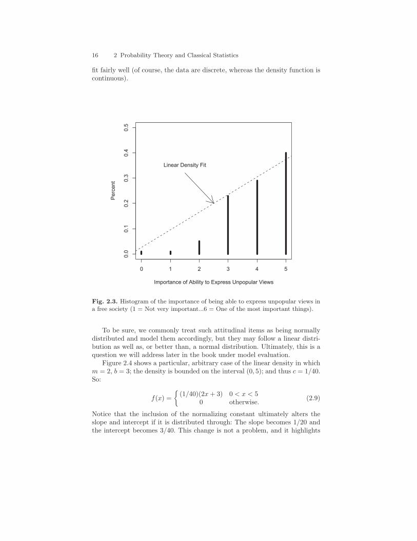
16 2 Probability Theory and Classical Statistics
fit fairly well (of course, the data are discrete, whereas the density function iscontinuous).
0 1 2 3 4 5
0.0
0.1
0.2
0.3
0.4
0.5
Importance of Ability to Express Unpopular Views
Perc
ent
Linear Density Fit
Fig. 2.3. Histogram of the importance of being able to express unpopular views ina free society (1 = Not very important...6 = One of the most important things).
To be sure, we commonly treat such attitudinal items as being normallydistributed and model them accordingly, but they may follow a linear distri-bution as well as, or better than, a normal distribution. Ultimately, this is aquestion we will address later in the book under model evaluation.
Figure 2.4 shows a particular, arbitrary case of the linear density in whichm = 2, b = 3; the density is bounded on the interval (0, 5); and thus c = 1/40.So:
f(x) =
{
(1/40)(2x+ 3) 0 < x < 50 otherwise.
(2.9)
Notice that the inclusion of the normalizing constant ultimately alters theslope and intercept if it is distributed through: The slope becomes 1/20 andthe intercept becomes 3/40. This change is not a problem, and it highlights
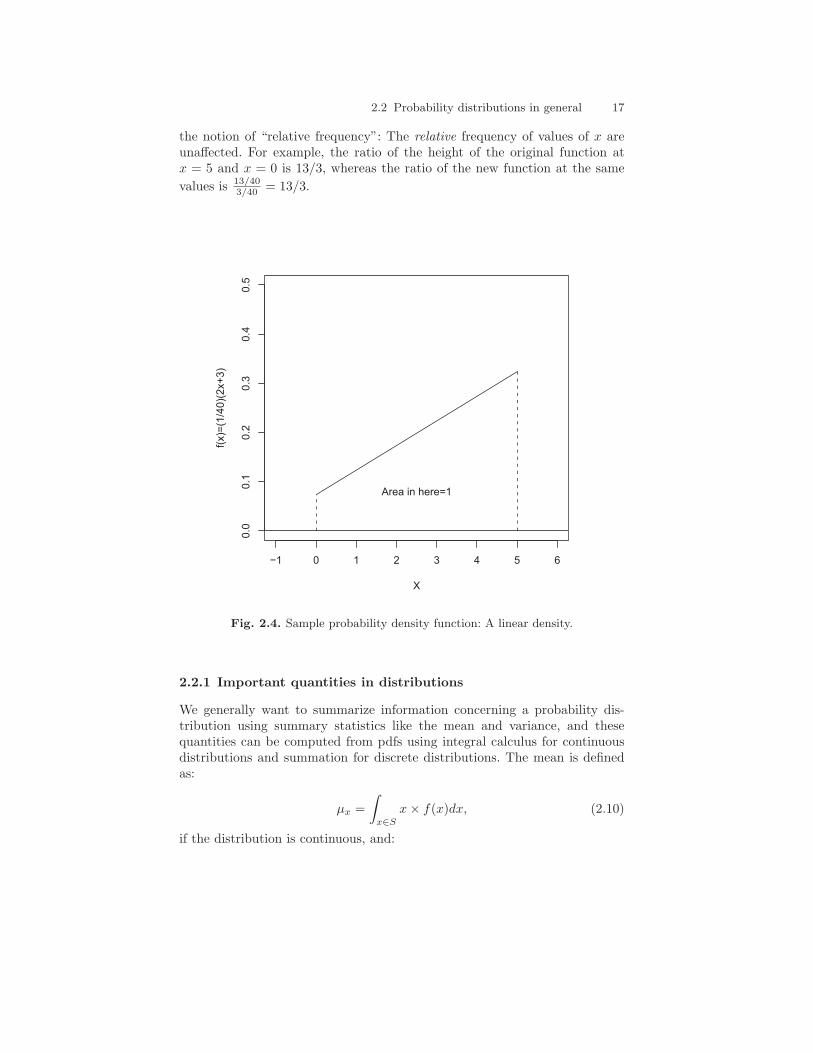
2.2 Probability distributions in general 17
the notion of “relative frequency”: The relative frequency of values of x areunaffected. For example, the ratio of the height of the original function atx = 5 and x = 0 is 13/3, whereas the ratio of the new function at the same
values is 13/403/40 = 13/3.
−1 0 1 2 3 4 5 6
0.0
0.1
0.2
0.3
0.4
0.5
X
f(x)=
(1/4
0)(
2x+
3)
Area in here=1
Fig. 2.4. Sample probability density function: A linear density.
2.2.1 Important quantities in distributions
We generally want to summarize information concerning a probability dis-tribution using summary statistics like the mean and variance, and thesequantities can be computed from pdfs using integral calculus for continuousdistributions and summation for discrete distributions. The mean is definedas:
µx =
∫
x∈S
x× f(x)dx, (2.10)
if the distribution is continuous, and:

18 2 Probability Theory and Classical Statistics
µx =∑
x∈S
x× p(x), (2.11)
if the distribution is discrete. The mean is often called the “expectation” orexpected value of x and is denoted as E(x). The variance is defined as:
σ2x =
∫
x∈S
(x− µx)2 × f(x)dx, (2.12)
if the distribution is continuous, and:
σ2x =
1
n
∑
x∈S
(x− µx)2, (2.13)
if the distribution is discrete. Using the expectation notation introduced forthe mean, the variance is sometimes referred to as E((x − µx)2); in otherwords, the variance is the expected value of the squared deviation from themean.2
Quantiles, including the median, can also be computed using integral cal-culus. The median of a continuous distribution, for example, is obtained byfinding Q that satisfies:
.5 =
∫ Q
−∞
f(x)dx. (2.14)
Returning to the examples in the previous section, the mean of the U(a, b)distribution is:
E(x) = µx =
∫ b
a
x×(
1
b− a
)
dx =b+ a
2,
and the variance is:
E((x− µx)2) =
∫ b
a
1
b− a(x− µx)2 dx =
(b− a)2
12.
For the linear density with the arbitrary parameter values introduced inEquation 2.9 (f(x) = (1/40)(2x+ 3)), the mean is:
µx =
∫ 5
0
x× (1/40)(2x+ 3)dx = (1/240)(4x3 + 9x2)dx
∣
∣
∣
∣
5
0
= 3.02.
The variance is:
2 The sample mean, unlike the population distribution mean shown here, is esti-mated with (n − 1) in the denominator rather than with n. This is a correctionfactor for the known bias in estimating the population variance from sample data.It becomes less important asymptotically (as n →∞.)

2.2 Probability distributions in general 19
Var(x) =
∫ 5
0
(x− 3.02)2 × (1/40)(2x+ 3)dx = 1.81.
Finally, the median can be found by solving for Q in:
.5 =
∫ Q
0
(1/40)(2x+ 3)dx.
This yields:20 = Q2 + 3Q,
which can be solved using the quadratic formula from algebra. The quadraticformula yields two real roots—3.22 and −6.22—only one of which is withinthe “support” of the distribution (3.22); that is, only one has a value thatfalls in the domain of the distribution.
In addition to finding particular quantiles of the distribution (like quartilecutpoints, deciles, etc.), we may also like to determine the probability associ-ated with a given range of the variable. For example, in the U(0,1) distribution,what is the probability that a random value drawn from this distribution willfall between .2 and .6? Determining this probability also involves calculus3:
p(.2 < x < .6) =
∫ .6
.2
1
1− 0dx = x
∣
∣
∣
∣
.6
.2
= .4.
An alternative, but equivalent, way of conceptualizing probabilities for regionsof a density is in terms of the cdf. That is, p(.2 < x < .6) = F (x = .6)−F (x =
.2), where F is∫X
0f(x)dx [the cumulative distribution function of f(x)].
2.2.2 Multivariate distributions
In social science research, we routinely need distributions that represent morethan one variable simultaneously. For example, factor analysis, structuralequation modeling with latent variables, simultaneous equation modeling, aswell as other methods require the simultaneous analysis of variables that arethought to be related to one another. Densities that involve more than onerandom variable are called joint densities, or more commonly, multivariatedistributions. For the sake of concreteness, a simple, arbitrary example ofsuch a distribution might be:
f(x, y) =
{
c(2x+ 3y + 2) if 0 < x < 2 , 0 < y < 20 otherwise.
(2.15)
Here, the x and y are the two dimensions of the random variable, and f(x, y)is the height of the density, given specific values for the two variables. Thus,
3 With discrete distributions, calculus is not required, only summation of the rele-vant discrete probabilities.

20 2 Probability Theory and Classical Statistics
f(x, y) gives us the relative frequency/probability of particular values of xand y. Once again, c is the normalizing constant that ensures the function ofx and y is a proper density function (that it integrates to 1). In this example,determining c involves solving a double integral:
c
∫ 2
0
∫ 2
0
(2x+ 3y + 2) dx dy = 1.
For this distribution, c = 1/28 (find this).Figure 2.5 shows this density in three dimensions. The height of the density
represents the relative frequencies of particular pairs of values for x and y. Asthe figure shows, the density is a partial plane (bounded at 0 and 2 in both xand y dimensions) that is tilted so that larger values of x and y occur morefrequently than smaller values. Additionally, the plane inclines more steeplyin the y dimension than the x dimension, given the larger slope in the densityfunction.
x
−0.50.0
0.51.0
1.5
2.0
2.5
y
−0.5
0.0
0.51.0
1.52.0
2.5
f(x,z
)
0.0
0.1
0.2
0.3
0.4
0.5
Fig. 2.5. Sample probability density function: A bivariate plane density.

2.2 Probability distributions in general 21
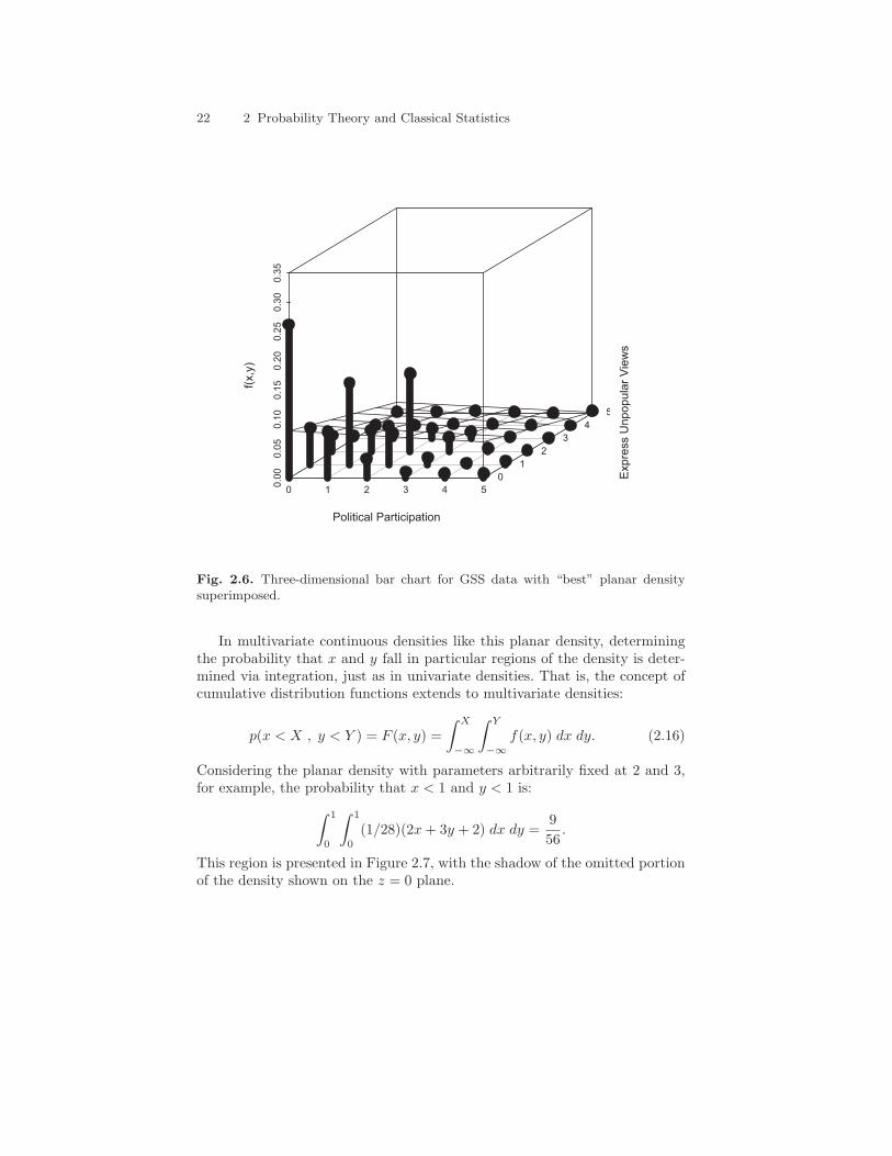
What pair of variables might follow a distribution like this one (albeitwith different parameters and domains)? Realistically, we probably would notuse this distribution, but some variables might actually follow this sort ofpattern. Consider two items from the 2000 GSS topic module on freedom: theone we previously discussed regarding the importance of the ability to expressunpopular views in a free society, and another asking respondents to classifythe importance of political participation to freedom. Table 2.1 is a cross-tabulation of these two variables. Considered separately, each variable followsa linear density such as discussed earlier. The proportion of individuals inthe “Most Important” category for each variable is large, with the proportiondiminishing across the remaining categories of the variable. Together, thevariables appear to some extent to follow a planar density like the one above.Of course, there are some substantial deviations in places, with two noticeable‘humps’ along the diagonal of the table.
Table 2.1. Cross-tabulation of importance of expressing unpopular views with im-portance of political participation.
Express Unpopular ViewsPolitical
Participation 1 2 3 4 5 6
1 361 87 39 8 2 2 36%
2 109 193 51 13 2 3 27%
3 45 91 184 25 4 5 26%
4 15 17 35 17 4 2 7%
5 10 4 9 5 2 0 2%
6 11 9 4 3 1 5 2%
40% 29% 23% 5% 1% 1% 100%
Note: Data are from the 2000 GSS special topic module on freedom (variables areexpunpop and partpol). 1 = One of the most important parts of freedom . . . 6 =Not so important to freedom.
Figure 2.6 presents a three-dimensional depiction of these data with an es-timated planar density superimposed. The imposed density follows the generalpattern of the data but fits poorly in several places. First, in several places theplanar density substantially underestimates the true frequencies (three placesalong the diagonal). Second, the density tends to substantially overestimatefrequencies in the middle of the distribution. Based on these problems, findingan alternative density is warranted. For example, a density with exponentialor quadratic components may be desirable in order to allow more rapid de-clines in the expected relative frequencies at higher values of the variables.Furthermore, we may consider using a density that contains a parameter—like a correlation—that captures the relationship between the two variables,given their apparent lack of independence (the “humps” along the diagonal).
22 2 Probability Theory and Classical Statistics
0 1 2 3 4 5
0.0
00.0
50.1
00.1
50.2
00.2
50.3
00.3
5
0
1
2
3
4
5
Political Participation
Expre
ss U
npopula
r V
iew
s
f(x,y
)
Fig. 2.6. Three-dimensional bar chart for GSS data with “best” planar densitysuperimposed.
In multivariate continuous densities like this planar density, determiningthe probability that x and y fall in particular regions of the density is deter-mined via integration, just as in univariate densities. That is, the concept ofcumulative distribution functions extends to multivariate densities:
p(x < X , y < Y ) = F (x, y) =
∫ X
−∞
∫ Y
−∞
f(x, y) dx dy. (2.16)
Considering the planar density with parameters arbitrarily fixed at 2 and 3,for example, the probability that x < 1 and y < 1 is:
∫ 1
0
∫ 1
0
(1/28)(2x+ 3y + 2) dx dy =9
56.
This region is presented in Figure 2.7, with the shadow of the omitted portionof the density shown on the z = 0 plane.

2.2 Probability distributions in general 23
x
−0.50.0
0.51.0
1.5
2.0
2.5
y
−0.5
0.0
0.51.0
1.52.0
2.5
f(x,z
)
0.0
0.1
0.2
0.3
0.4
0.5
Fig. 2.7. Representation of bivariate cumulative distribution function: Area underbivariate plane density from 0 to 1 in both dimensions.
2.2.3 Marginal and conditional distributions
Although determining the probabilities for particular regions of multivariatedensities is important, we may be interested in only a subset of the dimen-sions of a multivariate density. Two types of “subsets” are frequently needed:marginal distributions and conditional distributions. The data contained inTable 2.1 help differentiate these two types of distributions.
The marginal distribution for the “Express unpopular views” item is therow at the bottom of the table: It is the distribution of this variable summingacross the categories of the other variable (or integrating, if the density werecontinuous). The conditional distribution of this item, on the other hand,is the row of the table corresponding to a particular value for the politicalparticipation variable. For example, the conditional distribution for expressingunpopular views, given the value of “1” for political participation, consists ofthe data in the first row of the table (361, 87, 39, 8, 2, and 2, or in renormalizedpercents: 72%, 17%, 8%, 2%, .4%, and .4%).
24 2 Probability Theory and Classical Statistics
Thus, we can think of marginal distributions for a variable as being theoriginal distribution “flattened” in one dimension, whereas the conditionaldistribution for a variable is a “slice” through one dimension.
Finding marginal and conditional distributions mathematically is concep-tually straightforward, although often difficult in practice. Although Equa-tion 2.5 was presented in terms of discrete probabilities, the rule also appliesto density functions. From Equation 2.5, a conditional distribution can becomputed as:
f(x|y) =f(x, y)
f(y)(2.17)
This equation says that the conditional distribution for x given y is equal tothe joint density of x and y divided by the marginal distribution for y, where amarginal distribution is the distribution of one variable, integrating/summingover the other variables in the joint density. Thus:
f(y) =
∫
x∈S
f(x, y)dx. (2.18)
In terms of our bivariate distribution above (f(x, y) = (1/28)(2x+3y+2)),the marginal distributions for x and y can be found as:
f(x) =
∫ 2
y=0
(1/28)(2x+ 3y + 2)dy = (1/28)(4x+ 10)
and
f(y) =
∫ 2
x=0
(1/28)(2x+ 3y + 2)dx = (1/28)(6y + 8).
The conditional distributions can then be found as:
f(x|y) =(1/28)(2x+ 3y + 2)∫ 2
x=0(2x+ 3y + 2)dx
=(1/28)(2x+ 3y + 2)
(1/28)(6y + 8)
and
f(y|x) =(1/28)(2x+ 3y + 2)∫ 2
y=0(2x+ 3y + 2)dy
=(1/28)(2x+ 3y + 2)
(1/28)(4x+ 10).
Observe how the marginal distributions for each variable exclude the othervariable (as they should), whereas the conditional distributions do not. Once aspecific value for x or y is chosen in the conditional distribution, however, theremaining function will only depend on the variable of interest. Once again,in other words, the conditional distribution is akin to taking a slice throughone dimension of the bivariate distribution.
As a final example, take the conditional distribution f(x|y), where y = 0,so that we are looking at the slice of the bivariate distribution that lies on thex axis. The conditional distribution for that slice is:

2.3 Some important distributions in social science 25
f(x|y = 0) =2x+ 3(y = 0) + 2
6(y = 0) + 8= (1/8)(2x+ 2).
With very little effort, it is easy to see that this result gives us the formulafor the line that we observe in the x, z plane when we set y = 0 in the originalunnormalized function and we exclude the constant 1/8. In other words:
(1/8)(2x+ 2) ∝ (1/28)(2x+ 3y + 2)
when y = 0. Thus, an important finding is that the conditional distributionf(x|y) is proportional to the joint distribution for f(x, y) evaluated at a par-ticular value for y [expressed f(x|y) ∝ f(x, y)], differing only by a normalizingconstant. This fact will be useful when we discuss Gibbs sampling in Chap-ter 4.
2.3 Some important distributions in social science
Unlike the relatively simple distributions we developed in the previous sec-tion, the distributions that have been found to be most useful in social scienceresearch appear more complicated. However, it should be remembered that,despite their sometimes more complicated appearance, they are simply alge-braic functions that describe the relative frequencies of occurence for partic-ular values of a random variable. In this section, I discuss several of the mostimportant distributions used in social science research. I limit the discussionat this point to distributions that are commonly applied to random variablesas social scientists view them. In the next chapter, I discuss some additionaldistributions that are commonly used in Bayesian statistics as “prior distri-butions” for parameters (which, as we will see, are also treated as randomvariables by Bayesians). I recommend Evans, Hastings, and Peacock (2000)for learning more about these and other common probability distributions.
2.3.1 The binomial distribution
The binomial distribution is a common discrete distribution used in socialscience statistics. This distribution represents the probability for x successesin n trials, given a success probability p for each trial. If x ∼ Bin(n, p), then:
pr(x|n, p) =
(
nx
)
px(1− p)n−x. (2.19)
Here, I change the notation on the left side of the mass function to “pr”to avoid confusion with the parameter p in the function. The combinatorial,(
nx
)
, at the front of the function, compensates for the fact that the x suc-
cesses can come in any order in the n trials. For example, if we are interested

26 2 Probability Theory and Classical Statistics
in the probability of obtaining exactly 10 heads in 50 flips of a fair coin [thus,pr(x = 10 | n = 50, p = .5)], the 10 heads could occur back-to-back, or severalmay appear in a row, followed by several tails, followed by more heads, etc.This constant is computed as n!/(x!(n − x)!) and acts as a normalizing con-stant to ensure the mass under the curve sums to 1. The latter two terms inthe function multiply the independent success and failure probabilities, basedon the observed number of successes and failures. Once the parameters n andp are chosen, the probability of observing any number x of successes can becomputed/deduced. For example, if we wanted to know the probability of ex-
actly x = 10 heads out of n = 50 flips, then we would simply substitute thosenumbers into the right side of the equation, and the result would tell us theprobability. If we wanted to determine the probability of obtaining at least 10heads in 50 flips, we would need to sum the probabilities from 10 successes upto 50 successes. Obviously, in this example, the probability of obtaining moreheads than 50 or fewer heads than 0 is 0. Hence, this sample space is boundedto counting integers between 0 and 50, and computing the probability of atleast 10 heads would require summing 41 applications of the function (forx = 10, x = 11, ..., x = 50).
The mean of the binomial distribution is np, and the variance of the bi-nomial distribution is np(1 − p). When p = .5, the distribution is symmetricaround the mean. When p > .5, the distribution is skewed to the left; whenp < .5, the distribution is skewed to the right. See Figure 2.8 for an example ofthe effect of p on the shape of the distribution (n = 10). Note that, althoughthe figure is presented in a histogram format for the purpose of appearance(the densities are presented as lines), the distribution is discrete, and so 0probability is associated with non-integer values of x.
A normal approximation to the binomial may be used when p is close to.5 and n is large, by setting µx = np and σx =
√
np(1− p). For example,in the case mentioned above in which we were interested in computing theprobability of obtaining 10 or more heads in a series of 50 coin flips, computing41 probabilities with the function would be tedious. Instead, we could setµx = 25, and σx =
√
50(.5)(1− .5) = 3.54, and compute a z-score as z =(10−25)/(3.54) = −4.24. Recalling from basic statistics that there is virtually0 probability in the tail of the z distribution to the left of −4.24, we wouldconclude that the probability of obtaining at least 10 heads is practically 1,using this approximation. In fact, the actual probability of obtaining at least10 heads is .999988.
When n = 1, the binomial distribution reduces to another important dis-tribution called the Bernoulli distribution. The binomial distribution is oftenused in social science statistics as a building block for models for dichotomousoutcome variables like whether a Republican or Democrat will win an upcom-ing election, whether an individual will die within a specified period of time,etc.

2.3 Some important distributions in social science 27
0 2 4 6 8 10
0.0
0.1
0.2
0.3
0.4
0.5
x
pr(
x)
Bin(p=.2) Bin(p=.5) Bin(p=.8)
Fig. 2.8. Some binomial distributions (with parameter n = 10).
2.3.2 The multinomial distribution
The multinomial distribution is a generalization of the binomial distributionin which there are more than two outcome categories, and thus, there aremore than two “success” probabilities (one for each outcome category). Ifx ∼Multinomial(n, p1, p2, . . . , pk), then:
pr(x1 . . . xk | n, p1 . . . pk) =n!
x1! x2! . . . xk!px1
1 px2
2 . . . pxk
k , (2.20)
where the leading combinatorial expression is a normalizing constant,∑k
i=1 pi =
1, and∑k
i=1 xi = n. Whereas the binomial distribution allows us to computethe probability of obtaining a given number of successes (x) out of n trials,given a particular success probability (p), the multinomial distribution allowsus to compute the probability of obtaining particular sets of successes, givenn trials and given different success probabilities for each member of the set.To make this idea concrete, consider rolling a pair of dice. The sample space

28 2 Probability Theory and Classical Statistics
for possible outcomes of a single roll is S = {2, 3, 4, 5, 6, 7, 8, 9, 10, 11, 12}, andwe can consider the number of occurrences in multiple rolls of each of theseoutcomes to be represented by a particular x (so, x1 represents the numberof times a 2 is rolled, x2 represents the number of times a 3 is rolled, etc.).The success probabilities for these possible outcomes vary, given the fact thatthere are more ways to obtain some sums than others. The vector of prob-abilities p1 . . . p11 is { 1
36 ,236 ,
336 ,
436 ,
536 ,
636 ,
536 ,
436 ,
336 ,
236 ,
136}. Suppose we roll
the pair of dice 36 times. Then, if we want to know the probability of obtain-ing one “2”, two “3s”, three “4s”, etc., we would simply substitute n = 36,p1 = 1
36 , p2 = 236 , . . . , p11 = 1
36 , and x1 = 1, x2 = 2, x3 = 3, . . . into thefunction and compute the probability.
The multinomial distribution is often used in social science statistics tomodel variables with qualitatively different outcomes categories, like religiousaffiliation, political party affiliation, race, etc, and I will discuss this distribu-tion in more depth in later chapters as a building block of some generalizedlinear models and some multivariate models.
2.3.3 The Poisson distribution
The Poisson distribution is another discrete distribution, like the binomial,but instead of providing the probabilities for a particular number of successesout of a given number of trials, it essentially provides the probabilities for agiven number of successes in an infinite number of trials. Put another way,the Poisson distribution is a distribution for count variables. If x ∼ Poi(λ),then:
p(x|λ) =e−λλx
x!. (2.21)
Figure 2.9 shows three Poisson distributions, with different values for the λparameter. When λ is small, the distribution is skewed to the right, with mostof the mass concentrated close to 0. As λ increases, the distribution becomesmore symmetric and shifts to the right. As with the figure for the binomialdistribution above, I have plotted the densities as if they were continuous forthe sake of appearance, but because the distribution is discrete, 0 probabilityis associated with non-integer values of x
The Poisson distribution is often used to model count outcome variables,(e.g., numbers of arrests, number of children, etc.), especially those with lowexpected counts, because the distributions of such variables are often skewedto the right with most values clustered close to 0. The mean and variance of thePoisson distribution are both λ, which is often found to be unrealistic for manycount variables, however. Also problematic with the Poisson distribution isthe fact that many count variables, such as the number of times an individualis arrested, have a greater frequency of 0 counts than the Poisson densitypredicts. In such cases, the negative binomial distribution (not discussed here)and mixture distributions (also not discussed) are often used (see Degroot 1986

2.3 Some important distributions in social science 29
5 10 15 20
0.0
0.1
0.2
0.3
x
pr(
x | λ
)
λ=1
λ=3
λ=8
Fig. 2.9. Some Poisson distributions.
for the development of the negative binomial distribution; see Long 1997 fora discussion of negative binomial regression modeling; see Land, McCall, andNagin 1996 for a discussion of the use of Poisson mixture models).
2.3.4 The normal distribution
The most commonly used distribution in social science statistics and statisticsin general is the normal distribution. Many, if not most, variables of interestfollow a bell-shaped distribution, and the normal distribution, with both amean and variance parameter, fits such variables quite well. If x ∼ N(µ, σ2),then:
f(x|µ, σ) =1√
2πσ2exp
{
− (x− µ)2
2σ2
}
. (2.22)
In this density, the preceding (√
2πσ2)−1 is included as a normalizingconstant so that the area under the curve from −∞ to +∞ integrates to 1.The latter half of the pdf is the “kernel” of the density and gives the curve its
30 2 Probability Theory and Classical Statistics
location and shape. Given a value for the parameters of the distribution, µ andσ2, the curve shows the relative probabilities for every value of x. In this case,x can range over the entire real line, from −∞ to +∞. Technically, because aninfinite number of values exist between any two other values of x (ironicallymaking p(x = X) = 0,∀X), the value returned by the function f(x) does notreveal the probability of x, unlike with the binomial and Poisson distributionabove (as well as other discrete distributions). Rather, when using continuouspdfs, one must consider the probability for regions under the curve. Just asabove in the discussion of the binomial distribution, where we needed to sumall the probabilities between x = 10 and x = 50 to obtain the probabilitythat x ≥ 10, here we would need to integrate the continuous function fromx = a to x = b to obtain the probability that a < x < b. Note that we didnot say a ≤ x ≤ b; we did not for the same reason mentioned just above: Theprobability that x equals any number q is 0 (the area of a line is 0). Hencea < x < b is equivalent to a ≤ x ≤ b.
The case in which µ = 0 and σ2 = 1 is called the “standard normaldistribution,” and often, the z distribution. In that case, the kernel of thedensity reduces to exp
{
−x2/2}
, and the bell shape of the distribution canbe easily seen. That is, where x = 0, the function value is 1, and as x movesaway from 0 in either direction, the function value rapidly declines.
Figure 2.10 depicts three different normal distributions: The first has amean of 0 and a standard deviation of 1; the second has the same mean buta standard deviation of 2; and the third has a standard deviation of 1 but amean of 3.
The normal distribution is used as the foundation for ordinary least squares(OLS) regression, for some generalized linear models, and for many other mod-els in social science statistics. Furthermore, it is an important distribution instatistical theory: The Central Limit Theorem used to justify most of classicalstatistical testing states that sampling distributions for statistics are, in thelimit, normal. Thus, the z distribution is commonly used to assess statistical“significance” within a classical statistics framework. For these reasons, wewill consider the normal distribution repeatedly throughout the remainder ofthe book.
2.3.5 The multivariate normal distribution
The normal distribution easily extends to more than one dimension. If X ∼MVN(µ,Σ), then:
f(X|µ,Σ) = (2π)−k
2 |Σ|− 1
2 exp
{
−1
2(X − µ)TΣ−1(X − µ)
}
, (2.23)
where X is a vector of random variables, k is the dimensionality of the vector,µ is the vector of means of X, and Σ is the covariance matrix of X. Themultivariate normal distribution is an extension of the univariate normal in

2.3 Some important distributions in social science 31
−10 −5 0 5 10
0.0
0.1
0.2
0.3
0.4
0.5
x
f(x)
N(0,2)
N(0,1) N(3,1)
Fig. 2.10. Some normal distributions.
which x is expanded from a scalar to a k-dimensional vector of variables,x1, x2, . . . , xk, that are related to one another via the covariance matrix Σ.If X is multivariate normal, then each variable in the vector X is normal. IfΣ is diagonal (all off-diagonal elements are 0), then the multivariate normaldistribution is equivalent to k univariate normal densities.
When the dimensionality of the MVN distribution is equal to two, thedistribution is called the “bivariate normal distribution.” Its density function,although equivalent to the one presented above, is often expressed in scalarform as:
f(x1, x2) =1
2πσ1σ2
√
1− ρ2exp
[
− 1
2(1− ρ2)(Q−R+ S)
]
, (2.24)
where
Q =(x1 − µ1)
2
σ21
, (2.25)
R =2ρ(x1 − µ1)(x2 − µ2)
σ1σ2, (2.26)

32 2 Probability Theory and Classical Statistics
and
S =(x2 − µ2)
2
σ22
. (2.27)
The bivariate normal distribution, when the correlation parameter ρ is 0,looks like a three-dimensional bell. As ρ becomes larger (in either positive ornegative directions), the bell flattens, as shown in Figure 2.11. The upper partof the figure shows a three-dimensional view and a (top-down) contour plot ofthe bivariate normal density when ρ = 0. The lower part of the figure showsthe density when ρ = .8.
x1
x2
f(X | r=
0)
x1
x2
−3 −2 −1 0 1 2 3
−3
−1
12
3
x1
x2
f(X | r=
.8)
x1
x2
−3 −2 −1 0 1 2 3
−3
−1
12
3
Fig. 2.11. Two bivariate normal distributions.
2.4 Classical statistics in social science 33
The multivariate normal distribution is used fairly frequently in socialscience statistics. Specifically, the bivariate normal distribution is used tomodel simultaneous equations for two outcome variables that are known tobe related, and structural equation models rely on the full multivariate normaldistribution. I will discuss this distribution in more depth in later chaptersdescribing multivariate models.
2.3.6 t and multivariate t distributions
The t (Student’s t) and multivariate t distributions are quite commonly usedin modern social science statistics. For example, when the variance is un-known in a model that assumes a normal distribution for the data, with thevariance following an inverse gamma distribution (see subsequent chapters),the marginal distribution for the mean follows a t distribution (consider testsof coefficients in a regression model). Also, when the sample size is small, thet is used as a robust alternative to the normal distribution in order to com-pensate for heavier tails in the distribution of the data. As the sample sizeincreases, uncertainty about σ decreases, and the t distribution converges ona normal distribution (see Figure 2.12). The density functions for the t dis-tribution appears much more complicated than the normal. If x ∼ t(µ, σ, v),then:
f(x) =Γ ((v + 1)/2)
Γ (v/2)σ√vπ
(
1 + v−1
(
x− µ
σ
)2)−(v+1)/2
, (2.28)
where µ is the mean, σ is the standard deviation, and v is the “degrees offreedom.” If X is a k-dimensional vector of variables (x1 . . . xk), and X ∼mvt(µ,Σ, v), then:
f(X) =Γ ((v + d)/2)
Γ (v/2)vk/2πk/2| Σ |−1/2
(
1 + v−1(X − µ)TΣ−1(X − µ))−(v+k)/2
,
(2.29)where µ is a vector of means, and Σ is the variance-covariance matrix of X.
We will not explicitly use the t and multivariate t distributions in thisbook, although a number of marginal distributions we will be working withwill be implicitly t distributions.
2.4 Classical statistics in social science
Throughout the fall of 2004, CNN/USAToday/Gallup conducted a numberof polls attempting to predict whether George W. Bush or John F. Kerrywould win the U.S. presidential election. One of the key battleground stateswas Ohio, which ultimately George Bush won, but all the polls leading up

34 2 Probability Theory and Classical Statistics
−4 −2 0 2 4
0.0
0.1
0.2
0.3
0.4
0.5
x
f(x)
t(1 df)
t(2 df)
t(10 df)
t(120 df)
N(0,1) [solid line]
Fig. 2.12. The t(0, 1, 1), t(0, 1, 10), and t(0, 1, 120) distributions (with an N(0, 1)distribution superimposed).
to the election showed the two candidates claiming proportions of the votesthat were statistically indistinguishable in the state. The last poll in Ohioconsisted of 1,111 likely voters, 46% of whom stated that they would vote forBush, and 50% of whom stated that they would vote for Kerry, but the pollhad a margin of error of ±3%.4
In the previous sections, we discussed probability theory, and I statedthat statistics is essentially the inverse of probability. In probability, once weare given a distribution and its parameters, we can deduce the probabilitiesfor events. In statistics, we have a collection of events and are interested in
4 see http://www.cnn.com/ELECTION/2004/special/president/showdown/OH/polls.html for the data reported in this and the next chapter. Additional polls aredisplayed on the website, but I use only the CNN/USAToday/Gallup polls, giventhat they are most likely similar in sample design. Unfortunately, the proportionsare rounded, and so my results from here on are approximate. For example, inthe last poll, 50% planned to vote for Kerry, and 50% of 1,111 is 556. However,the actual number could range from 550 to 561 given the rounding.
2.5 Maximum likelihood estimation 35
determining the values of the parameters that produced them. Returning tothe polling data, determining who would win the election is tantamount todetermining the population parameter (the proportion of actual voters whowill vote for a certain candidate) given a collection of events (a sample ofpotential votes) thought to arise from this parameter and the probabilitydistribution to which it belongs.
Classical statistics provides one recipe for estimating this population pa-rameter; in the remainder of this chapter, I demonstrate how. In the nextchapter, I tackle the problem from a Bayesian perspective. Throughout thissection, by “classical statistics” I mean the approach that is most commonlyused among academic researchers in the social sciences. To be sure, the clas-sical approach to statistics in use is a combination of several approaches,involving the use of theorems and perspectives of a number of statisticians.For example, the most common approach to model estimation is maximumlikelihood estimation, which has its roots in the works of Fisher, whereas thecommon approach to hypothesis testing using p-values has its roots in theworks of both Neyman and Pearson and Fisher—each of whom in fact devel-oped somewhat differing views of hypothesis testing using p-values (again, seeHubbard and Bayarri 2003 or see Gill 2002 for an even more detailed history).
2.5 Maximum likelihood estimation
The classical approach to statistics taught in social science statistics coursesinvolves two basic steps: (1) model estimation and (2) inference. The first stepinvolves first determining an appropriate probability distribution/model forthe data at hand and then estimating its parameters. Maximum likelihood(ML) is the most commonly used method of estimating parameters and de-termining the extent of error in the estimation (steps 1 and 2, respectively) insocial science statistics (see Edwards 1992 for a detailed, theoretical discus-sion of likelihood analysis; see Eliason 1993 for a more detailed discussion ofthe mechanics of ML estimation).
The fundamental idea behind maximum likelihood estimation is that agood choice for the estimate of a parameter of interest is the value of theparameter that makes the observed data most likely to have occurred. To dothis, we need to establish some sort of function that gives us the probabilityfor the data, and we need to find the value of the parameter that maximizesthis probability. This function is called the “likelihood function” in classicalstatistics, and it is essentially the product of sampling densities—probabilitydistributions—for each observation in the sample. The process of estimationthus involves the following steps:
1. Construct a likelihood function for the parameter(s) of interest.2. Simplify the likelihood function and take its logarithm.3. Take the partial derivative of the log-likelihood function with respect to
each parameter, and set the resulting equation(s) equal to 0.

36 2 Probability Theory and Classical Statistics
4. Solve the system of equations to find the parameters.
This process seems complicated, and indeed it can be. Step 4 can be quitedifficult when there are lots of parameters. Generally, some sort of iterativemethod is required to find the maximum. Below I detail the process of MLestimation.
2.5.1 Constructing a likelihood function
If x1, x2 . . . xn are independent observations of a random variable, x, in a dataset of size n, then we know from the multiplication rule in probability theorythat the joint probability for the vector X is:
f(X|θ) ≡ L(θ | x) =n∏
i=1
f(xi | θ). (2.30)
This equation is the likelihood function for the model. Notice how theparameter and the data switch places in the L(.) notation versus the f(.)notation. We denote this as L(.), because from a classical standpoint, theparameter is assumed to be fixed. However, we are interested in estimatingthe parameter θ, given the data we have observed, so we use this notation.The primary point of constructing a likelihood function is that, given the dataat hand, we would like to solve for the value of the parameter that makesthe occurence of the data most probable, or most “likely” to have actuallyoccurred.
As the right-hand side of the equation shows, the construction of the like-lihood function first relies on determining an appropriate probability distri-bution f(.) thought to generate the observed data. In our election pollingexample, the data consist of 1,111 potential votes, the vast majority of whichwere either for Bush or for Kerry. If we assume that candidates other thanthese two are unimportant—that is, the election will come down to whomamong these two receives more votes—then the data ultimately reduce to 556potential votes for Kerry and 511 potential votes for Bush. An appropriatedistribution for such data is the binomial distribution. If we are interestedin whether Kerry will win the election, we can consider a vote for Kerry a“success,” and its opposite, a vote for Bush, a “failure,” and we can set upour likelihood function with the goal of determining the success probabilityp. The likelihood function in this case looks like:
L(p|X) =
(
1067556
)
p556(1− p)511.
As an alternative view that ultimately produces the same results, we can con-sider that, at the individual level, each of our votes arises from a Bernoulli dis-tribution, and so our likelihood function is the product of n = 1, 067 Bernoullidistributions. In that case:
2.5 Maximum likelihood estimation 37
L(p|X) =n=1067∏
i=1
pxi(1− p)1−xi . (2.31)
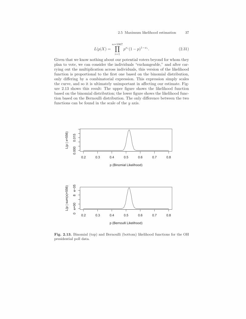
Given that we know nothing about our potential voters beyond for whom theyplan to vote, we can consider the individuals “exchangeable,” and after car-rying out the multiplication across individuals, this version of the likelihoodfunction is proportional to the first one based on the binomial distribution,only differing by a combinatorial expression. This expression simply scalesthe curve, and so it is ultimately unimportant in affecting our estimate. Fig-ure 2.13 shows this result: The upper figure shows the likelihood functionbased on the binomial distribution; the lower figure shows the likelihood func-tion based on the Bernoulli distribution. The only difference between the twofunctions can be found in the scale of the y axis.
0.2 0.3 0.4 0.5 0.6 0.7 0.8
0.0
00
0.0
15
p (Binomial Likelihood)
L(p
| x
=556)
0.2 0.3 0.4 0.5 0.6 0.7 0.8
0
e+
00
8
e−
05
p (Bernoulli Likelihood)
L(p
| s
um
(x)=
556)
Fig. 2.13. Binomial (top) and Bernoulli (bottom) likelihood functions for the OHpresidential poll data.
38 2 Probability Theory and Classical Statistics
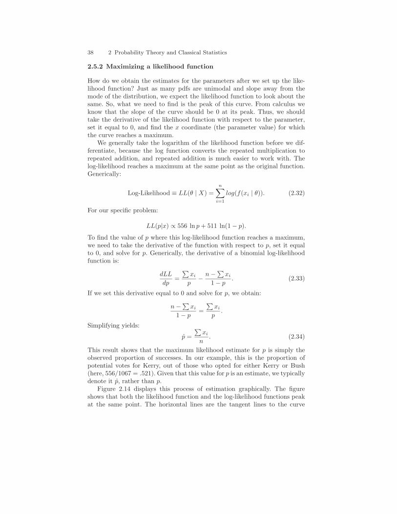
2.5.2 Maximizing a likelihood function
How do we obtain the estimates for the parameters after we set up the like-lihood function? Just as many pdfs are unimodal and slope away from themode of the distribution, we expect the likelihood function to look about thesame. So, what we need to find is the peak of this curve. From calculus weknow that the slope of the curve should be 0 at its peak. Thus, we shouldtake the derivative of the likelihood function with respect to the parameter,set it equal to 0, and find the x coordinate (the parameter value) for whichthe curve reaches a maximum.
We generally take the logarithm of the likelihood function before we dif-ferentiate, because the log function converts the repeated multiplication torepeated addition, and repeated addition is much easier to work with. Thelog-likelihood reaches a maximum at the same point as the original function.Generically:
Log-Likelihood ≡ LL(θ | X) =n∑
i=1
log(f(xi | θ)). (2.32)
For our specific problem:
LL(p|x) ∝ 556 ln p+ 511 ln(1− p).
To find the value of p where this log-likelihood function reaches a maximum,we need to take the derivative of the function with respect to p, set it equalto 0, and solve for p. Generically, the derivative of a binomial log-likelihoodfunction is:
dLL
dp=
∑
xi
p− n−∑xi
1− p. (2.33)
If we set this derivative equal to 0 and solve for p, we obtain:
n−∑xi
1− p=
∑
xi
p.
Simplifying yields:
p̂ =
∑
xi
n. (2.34)
This result shows that the maximum likelihood estimate for p is simply theobserved proportion of successes. In our example, this is the proportion ofpotential votes for Kerry, out of those who opted for either Kerry or Bush(here, 556/1067 = .521). Given that this value for p is an estimate, we typicallydenote it p̂, rather than p.
Figure 2.14 displays this process of estimation graphically. The figureshows that both the likelihood function and the log-likelihood functions peakat the same point. The horizontal lines are the tangent lines to the curve
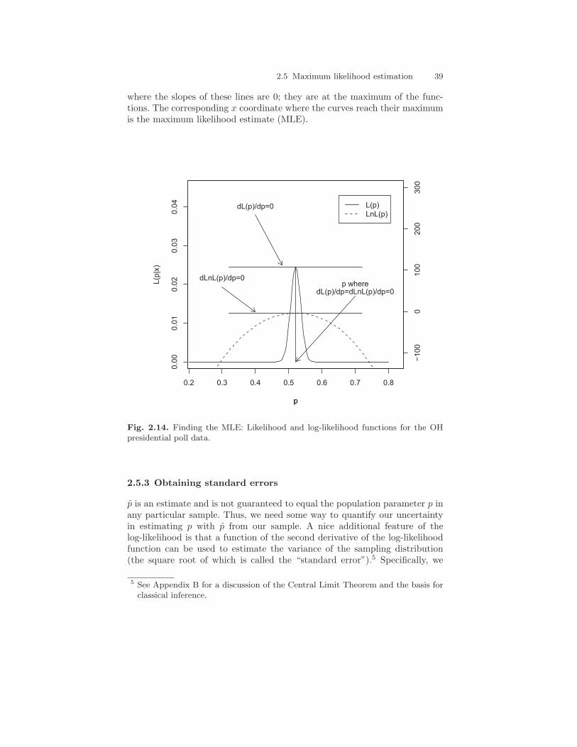
2.5 Maximum likelihood estimation 39
where the slopes of these lines are 0; they are at the maximum of the func-tions. The corresponding x coordinate where the curves reach their maximumis the maximum likelihood estimate (MLE).
0.2 0.3 0.4 0.5 0.6 0.7 0.8
0.0
00.0
10.0
20.0
30.0
4
p
L(p
|x)
dL(p)/dp=0
p wheredL(p)/dp=dLnL(p)/dp=0
p
−100
0100
200
300
dLnL(p)/dp=0
L(p)
LnL(p)
Fig. 2.14. Finding the MLE: Likelihood and log-likelihood functions for the OHpresidential poll data.
2.5.3 Obtaining standard errors
p̂ is an estimate and is not guaranteed to equal the population parameter p inany particular sample. Thus, we need some way to quantify our uncertaintyin estimating p with p̂ from our sample. A nice additional feature of thelog-likelihood is that a function of the second derivative of the log-likelihoodfunction can be used to estimate the variance of the sampling distribution(the square root of which is called the “standard error”).5 Specifically, we
5 See Appendix B for a discussion of the Central Limit Theorem and the basis forclassical inference.

40 2 Probability Theory and Classical Statistics
must take the inverse of the negative expected value of the second derivativeof the log-likelihood function. Mathematically:
I(θ)−1 =
(
−E(
∂2LL
∂θ∂θT
))−1
, (2.35)
where θ is our parameter or vector of parameters and I(θ) is called the “infor-mation matrix.” The square root of the diagonal elements of this matrix arethe parameter standard errors. I(θ)−1 can be computed using the followingsteps:
1. Take the second partial derivatives of the log-likelihood. In multiparametermodels, this produces a matrix of partial derivatives (called the Hessianmatrix).
2. Take the negative of the expectation of this matrix to obtain the “infor-mation matrix” I(θ).
3. Invert this matrix to obtain estimates of the variances and covariances ofparameters (get standard errors by square-rooting the diagonal elementsof the matrix).
The fact that I(θ)−1 contains the standard errors is not intuitive. But,if you recall that the first derivative is a measure of the slope of a functionat a point (the rate of change in the function at that point), and the secondderivative is a measure of the rate of change in the slope, we can think ofthe second derivative as indicating the rate of curvature of the curve. A verysteep curve, then, has a very high rate of curvature, which makes its secondderivative large. Thus, when we invert it, it makes the standard deviationsmall. On the other hand, a very shallow curve has a very low rate of curvature,which makes its second derivative small. When we invert a small number, itmakes the standard deviation large. Note that, when we evaluate the secondderivative, we substitute the MLE estimate for the parameter into the resultto obtain the standard error at the estimate.
Returning to our data at hand, the second partial derivative of the genericbinomial log-likelihood function with respect to p is:
∂2LL
∂p2=
∑
x
p2− n−
∑
x
(1− p)2. (2.36)
Taking expectations yields:
E
(
∂2LL
∂p2
)
= E
[
−∑
x
p2− n−∑x
(1− p)2
]
.
The expectation of these expressions can be computed by realizing that theexpectation of
∑
x/n is p (put another way: E(p̂) = p). Thus:
E
(
∂2LL
∂p2
)
= −npp2− n− np
(1− p)2.

2.5 Maximum likelihood estimation 41
Some simplification yields:
E
(
∂2LL
∂p2
)
= − n
p(1− p).
At this point, we can negate the expectation, invert it, and evaluate it at theMLE (p̂) to obtain:
I(p)−1 =p̂(1− p̂)
n. (2.37)
Taking the square root of this yields the estimated standard error. In ourpolling data case, the standard error is
√
(.521× .479)/1067 = .015.Recall that our question is whether Kerry would win the vote in Ohio. Our
estimate for the Ohio population proportion to vote for Kerry (versus Bush)was .521, which suggests he would win the popular vote in Ohio (discountingthird party candidates). However, the standard error of this estimate was.015. We can construct our usual confidence interval around the maximumlikelihood estimate to obtain a 95% interval for the MLE. If we do this, weobtain an interval of [.492, .550] (CI = p̂ ± 1.96 × s.e.(p̂)). Given that thelower bound on this interval is below .5, we can conclude that we cannot ruleout the possibility that Kerry would not win the popular vote in Ohio.
An alternative to the confidence interval approach to answering this ques-tion is to construct a t test, with a null hypothesis H0 : p < .5. Following thatapproach:
t =(.521− .5)
.015= 1.4.
This t value is not large enough to reject the null hypothesis (that Kerry’sproportion of the vote is less than .5), and thus, the conclusion we would reachis the same: We do not have enough evidence to conclude that Kerry will win(see Appendix B for more discussion of null hypotheses, confidence intervals,and t tests).
Note that this result is consistent with the result I stated at the beginningof this section: The results of the original poll suggested that the vote wastoo close to call, given a ±3% margin of error. Here, I have shown essentiallyfrom where that margin of error arose. We ended up with a margin of errorof .0294, which is approximately equal to the margin of error in the originalpoll.
2.5.4 A normal likelihood example
Because the normal distribution is used repeatedly throughout this book andthroughout the social sciences, I conclude this chapter by deriving parameterestimates and standard errors for a normal distribution problem. I keep thisexample at a general level; in subsequent chapters, we will return to thislikelihood function with specific problems and data.

42 2 Probability Theory and Classical Statistics
Suppose you have n observations x1, x2, . . . , xn that you assume are nor-mally distributed. Once again, if the observations are assumed to be indepen-dent, a likelihood function can be constructed as the multiple of independentnormal density functions:
L(µ, σ | X) =n∏
i=1
1√2πσ2
exp
{
− (xi − µ)2
2σ2
}
. (2.38)
We can simplify the likelihood as:
L(µ, σ | X) = (2πσ2)−n
2 exp
{
− 1
2σ2
n∑
i=1
(xi − µ)2
}
.
The log of the likelihood is:
LL(µ, σ | X) ∝ −n ln(σ)− 1
2σ2
n∑
i=1
(xi − µ)2. (2.39)
In the above equation, I have eliminated the −n2 log(2π), an irrelevant con-
stant. It is irrelevant, because it does not depend on either parameter andwill therefore drop once the partial derivatives are taken. In this example, wehave two parameters, µ and σ, and hence the first partial derivative must betaken with respect to each parameter. This will leave us with two equations(one for each parameter). After taking the partial derivatives with respect toeach parameter, we obtain the following:
∂LL
∂µ=n(x̄− µ)
σ2
and∂LL
∂σ= −n
σ+
1
σ3
n∑
i=1
(xi − µ)2.
Setting these partial derivatives each equal to 0 and doing a little algebrayields:
µ̂ = x̄ (2.40)
and
σ̂2 =
∑ni=1(xi − µ)2
n. (2.41)
These estimators should look familiar: The MLE for the population mean isthe sample mean; the MLE for the population variance is the sample variance.6
Estimates of the variability in the estimates for the mean and standarddeviation can be obtained as we did in the binomial example. However, as
6 The MLE is known to be biased, and hence, a correction is added, so that thedenominator is n− 1 rather than n.

2.5 Maximum likelihood estimation 43
noted above, given that we have two parameters, our second derivate matrixwill, in fact, be a matrix. For the purposes of avoiding taking square rootsuntil the end, let τ = σ2, and we’ll construct the Hessian matrix in terms ofτ . Also, let θ be a vector containing both µ and τ . Thus, we must compute:
∂2LL
∂θ∂θT=
∂2LL∂µ2
∂2LL∂µ∂τ
∂2LL∂τ∂µ
∂2LL∂τ2
. (2.42)
Without showing all the derivatives (see Exercises), the elements of the Hes-sian matrix are then:
∂2LL
∂θ∂θT=
−nτ −n(x̄−µ)
τ2
−n(x̄−µ)τ2
n2τ2 −
P
n
i=1(xi−µ)2
τ3
.
In order to obtain the information matrix, which can be used to compute thestandard errors, we must take the expectation of this Hessian matrix and takeits negative. Let’s take the expectation of the off-diagonal elements first. Theexpectation of x̄− µ is 0 (given that the MLE is unbiased), which makes theoff-diagonal elements of the information matrix equal to 0. This result shouldbe somewhat intuitive: There need be no relationship between the mean andvariance in a normal distribution.
The first element, (−n/τ), is unchanged under expectation. Thus, aftersubstituting σ2 back in for τ and negating the result, we obtain n/σ2 for thiselement of the information matrix.
The last element, (n/2τ2) − (∑n
i=1(xi − µ)2)/τ3, requires a little con-sideration. The only part of this expression that changes under expecta-tion is
∑ni=1(xi − µ)2. The expectation of this expression is nτ . That is,
E(xi − µ)2 = τ , and we are taking this value n times (notice the summa-tion). Thus, this element, after a little algebraic manipulation, negation, andsubstitution of σ2 for τ , becomes: n/2σ4. So, our information matrix appearsas:
I(θ) =
[
nσ2 00 n
2σ4
]
. (2.43)
To obtain standard errors, we need to (1) invert this matrix, and (2) takethe square root of the diagonal elements (variances) to obtain the standarderrors. Matrix inversion in this case is quite simple, given that the off-diagonalelements are equal to 0. In this case, the inverse of the matrix is simply theinverse of the diagonal elements.
Once we invert and square root the elements of the information matrix,we find that the estimate for the standard error for our estimate µ̂ is σ̂/
√n,
and our estimate for the standard error for σ̂2 is σ̂2√
2/n. The estimate forthe standard error for µ̂ should look familiar: It is the standard deviation of
44 2 Probability Theory and Classical Statistics
the sampling distribution for a mean based on the Central Limit Theorem(see Appendix B).
2.6 Conclusions
In this chapter, we have reviewed the basics of probability theory. Importantly,we have developed the concept of probability distributions in general, and wehave discussed a number of actual probability distributions. In addition, wehave discussed how important quantities like the mean and variance can bederived analytically from probability distributions. Finally, we reviewed themost common approach to estimating such quantities in a classical setting—maximum likelihood estimation—given a collection of data thought to arisefrom a particular distribution. As stated earlier, I recommend reading De-Groot (1986) for a more thorough introduction to probability theory, and Irecommend Billingsley (1995) and Chung and AitSahlia (2003) for more ad-vanced and detailed expositions. For a condensed exposition, I suggest Rudas2004. Finally, I recommend Edwards (1992) and Gill (2002) for detailed dis-cussions of the history and practice of maximum likelihood (ML) estimation,and I suggest Eliason (1993) for a highly applied perspective on ML estima-tion. In the next chapter, we will discuss the Bayesian approach to statisticsas an alternative to this classical approach to model building and estimation.
2.7 Exercises
2.7.1 Probability exercises
1. Find the normalizing constant for the linear density in Equation 2.8.2. Using the binomial mass function, find the probability of obtaining 3 heads
in a row with a fair coin.3. Find the probability of obtaining 3 heads in a row with a coin weighted
so that the probability of obtaining a head is .7.4. What is the probability of obtaining 3 heads OR 3 tails in a row with a
fair coin?5. What is the probability of obtaining 3 heads and 1 tail (order irrelevant)
on four flips of a fair coin?6. Using a normal approximation to the binomial distribution, find the prob-
ability of obtaining 130 or more heads in 200 flips of a fair coin.7. Plot a normal distribution with parameters µ = 5 and σ = 2.8. Plot a normal distribution with parameters µ = 2 and σ = 5.9. Plot the t(0, 1, df = 1) and t(0, 1, df = 10) distributions. Note: Γ is a
function. The function is: Γ (n) =∫∞
0e−uun−1du. For integers, Γ (n) =
(n − 1)! Thus, Γ (4) = (4 − 1)! = 6. However, when the argument to thefunction is not an integer, this formula will not work. Instead, it is easierto use a software package to compute the function value for you.

2.7 Exercises 45
10. Show that the multivariate normal density function reduces to the univari-ate normal density function when the dimensionality of the distributionis 1.
2.7.2 Classical inference exercises
1. Find the MLE for p in a binomial distribution representing a sample inwhich 20 successes were obtained out of 30 trials.
2. Based on the binomial sample in the previous question, if the trials in-volved coin flips, would having 20 heads be sufficient to question the fair-ness of the coin? Why or why not?
3. Suppose a sample of students at a major university were given an IQ test,which resulted in a mean of 120 and a standard deviation of 10. If weknow that IQs are normally distributed in the population with a mean of100 and a standard deviation of 16, is there sufficient evidence to suggestthat the college students are more intelligent than average?
4. Suppose a single college student were given an IQ test and scored 120. Isthere sufficient evidence to indicate that college students are more intelli-gent than average based on this sample?
5. What is the difference (if any) between the responses to the previous twoquestions?
6. Derive the Hessian matrix for the normal distribution example at the endof the chapter.
7. Derive the MLE for λ from a sample of n observations from a Poissondistribution.
8. Derive the standard error estimate for λ from the previous question.