Embed Size (px)
Citation preview

A Method for Simultaneous Variable Selection and
Outlier Identi�cation in Linear Regression�
Computational Statistics and Data Analysis
(1996),22, 251-270.
Jennifer Hoeting
Colorado State University
Adrian E. Raftery David Madigan
University of Washington
March 1, 1996
Abstract
We suggest a method for simultaneous variable selection and outlier identi�cation
based on the computation of posterior model probabilities. This avoids the problem
that the model you select depends upon the order in which variable selection and outlier
identi�cation are carried out. Our method can �nd multiple outliers and appears to
be successful in identifying masked outliers.
We also address the problem of model uncertainty via Bayesian model averaging.
For problems where the number of models is large, we suggest a Markov chain Monte
Carlo approach to approximate the Bayesian model average over the space of all possi-
ble variables and outliers under consideration. Software for implementing this approach
is described. In an example, we show that model averaging via simultaneous variable
selection and outlier identi�cation improves predictive performance and provides more
accurate prediction intervals as compared with any single model that might reasonably
be selected.
Key Words: Bayesian model averaging; Markov chain Monte Carlo model com-
position; Masking; Model uncertainty; Posterior model probability.
�Jennifer Hoeting is Assistant Professor of Statistics at the Department of Statistics, Colorado State
University, Fort Collins, CO 80523 (e-mail: [email protected]). Adrian E. Raftery is Professor of
Statistics and Sociology and David Madigan is Assistant Professor of Statistics at the Department of Statis-
tics, Box 354322, University of Washington, Seattle, WA 98195. The research of Raftery and Hoeting was
partially supported by ONR Contract N-00014-91-J-1074. Madigan's research was partially supported by
NSF grant no. DMS 92111627.
1

1 Introduction
Many approaches for the selection of variables and the identi�cation of outliers have been
proposed. Most authors focus on these problems separately. Adams (1991) and Blettner
and Sauerbrei (1993) pointed out that the model that is selected depends upon the order in
which variable selection and outlier identi�cation are performed. In this paper we de�ne a
model as a set of variables and a set of observations identi�ed as outliers.
Another di�culty in outlier identi�cation is masking, where multiple outliers in a data
set conceal the presence of additional outliers. Several authors have suggested methods to
overcomemasking, including Atkinson (1986a) and Hadi (1992), but these methods typically
involve removing the `masking' outliers from the data set before the `masked' outliers can
be identi�ed.
We o�er a simultaneous approach to variable selection and outlier identi�cation based
on Bayesian posterior model probabilities. \Simultaneous Bayesian Variable Selection and
Outlier Identi�cation" (SVO) overcomes the problem that order of methods in uences the
choice of outliers and variables. SVO includes a method for identifying multiple outliers
which appears to be successful in the identi�cation of masked outliers.
We also consider the problem of model uncertainty in linear regression. The typical
approach to model selection involves choosing a single set of variables and identifying a
single set of observations as outliers. Subsequent inferences ignore uncertainty involved in the
selection of the model. A complete Bayesian solution to this problem involves averaging over
all possible models when making inferences about quantities of interest. Indeed, Bayesian
model averaging provides optimal predictive ability (Madigan and Raftery 1994). In many
applications however, this approach will not be practical due to the large number of models
for which posteriors need to be computed.
To overcome this problem we suggest a Markov chain Monte Carlo approach to approx-
imate the Bayesian model average for the space of all possible variables and outliers under
consideration. Markov chain Monte Carlo model composition (MC3) was originally pro-
posed by Madigan and York (1995) and was adapted for linear regression models by Raftery,
Madigan, and Hoeting (1994). We show in an example that model averaging via MC3 pro-
vides better predictive performance than any single model which might reasonably have been
selected. Software for implementing MC3 is described.
In the next section we discuss various approaches to outlier identi�cation. In Section 3 we
outline our method for SVO including our method for the identi�cation of multiple outliers.
In Section 4 we provide two examples using SVO. In Section 5 we summarize Bayesian model
averaging and outline MC3 as implemented for the simultaneous approach. We also discuss
the assessment of predictive performance and provide an example comparing the predictive
performance of BMA to the predictive performance of single models that would have been
chosen using standard techniques. Conclusions are given in Section 6. In the Appendix we
describe software for implementing MC3.
2

2 Outliers in Linear Regression
Observations that do not follow the same model as the rest of the data are typically called
outliers. There is a vast literature on methods for handling outliers including at least three
books (Rousseeuw and Leroy 1987, Barnett and Lewis 1994, and Hawkins 1980). Outliers
are typically modeled by either a shift in mean (i.e., for an outlier yi, let yj = Xj� + �j for
all j 6= i and let yi = Xi� + � + �i) or via a shift in variance (described in Section 3.1). The
mean-slippage model is typically used to identify outliers to make them available for further
study. The variance{in ation model is often adopted for robust techniques with the aim of
tolerating or accommodating outliers. We have adopted the variance{in ation model in this
work.
Many methods have been suggested for detecting single outliers. For a comparison of
many of the available methods, see Chatterjee and Hadi (1986). Bayesian outlier models
have also been much discussed in the literature, including Box and Tiao (1968), Guttman et
al. (1978), Verdinelli and Wasserman (1991), and Pettit (1992).
If a data set has multiple outliers, then the outliers may mask one another making outlier
identi�cation di�cult. If masked outliers are not removed from the model as a group, their
presence goes undetected. An obvious solution to this problem, the computationally inten-
sive task of consideration of all subsets of observations to be potential outliers, is typically
impossible to carry out due to the large number of subsets to be considered.
Several authors have suggested algorithms for detecting multiple outliers including Hadi
(1990), Kianifard and Swallow (1989) and Marasinghe (1985). There are also robust methods
which produce coe�cient estimates that are consistent with the majority of the data. These
include work by Rousseeuw (1984), Heiberger and Becker (1991), and Bloom�eld and Steiger
(1983).
The method we use to identify multiple outliers involves two steps. In a �rst exploratory
step we use a robust technique to identify a set of potential outliers. The robust approach
typically identi�es a large number of potential outliers. In the second step, we compute
all possible posterior model probabilities or use MC3, considering all possible subsets of the
set of potential outliers. This two{step method is computationally feasible, and it allows for
groups of observations to be considered simultaneously as potential outliers. In the examples
we have considered to date, our method successfully identi�es masked outliers. We describe
the method in detail below.
3

3 Simultaneous Variable Selection and Outlier Identi-
�cation
3.1 Bayesian Framework and Selection of Prior Distributions
We adopt a variance{in ation model for outliers as follows: Let Y = X� + � where the
observed data on the predictors are contained in the n� (p+1) matrix X and the observed
data on the dependent variable are contained in the n-vector Y . We assume that the �'s in
distinct cases are independent where
� �
(N(0; �2) w:p: (1� �)
N (0;K2�2) w:p: �:(1)
Here � is the probability of an outlier and K2 is the variance{in ation parameter.
We typically consider all models equally likely a priori and the (p+1) parameter vector �
and �2 to be unknown. Where possible, informative prior distributions for � and �2 should
be elicited and incorporated into the analysis|see Kadane et al. (1980) and Garthwaite
and Dickey (1992). In the absence of expert opinion we seek prior distributions which re ect
uncertainty about the parameters and also embody reasonable a priori constraints. We use
prior distributions that are proper but reasonably at over the range of parameter values
that could plausibly arise. These represent the common situation where there is some prior
information, but rather little of it. We use the standard normal-gamma conjugate class of
priors,
� � N(�; �2V );
��
�2� �2�:
Here �, �, the (p + 1) � (p + 1) matrix V and the (p + 1)-vector � are hyperparameters to
be chosen.
For non-categorical predictor variables we assume the individual �'s to be independent a
priori. We center the distribution of � on zero (apart from �0) and choose � = (�̂0; 0; 0; : : : ; 0)
where �̂0 is the ordinary least squares estimate of �0. The covariance matrix V is diagonal
with entries (s2Y ; �2s�21 ; �2s�22 ; : : : ; �2s�2p ) where s2Y denotes the sample variance of Y , s2i
denotes the sample variance of Xi for i = 1; : : : ; p, and � is a hyperparameter to be chosen.
The prior variance of �0 is chosen conservatively and represents an upper bound on the
reasonable variance for this parameter. The variances of the remaining �-parameters are
chosen to re ect increasing precision about each �i as the variance of the corresponding Xi
increases and to be invariant to scale changes in both the predictor variables and the response
variable. For details of our treatment of categorical predictor variables, see Hoeting (1994).
The marginal distribution of the response y based on the proper priors discussed above
is a non-central Student's t distribution with � degrees of freedom, mean X�, and vari-
4

ance [�=(� � 2)]� (� +XV X t) where � is a diagonal matrix with K2 on the diagonal for
observations identi�ed to be outliers and 1's elsewhere.
3.2 Choosing Hyperparameter Values for the Prior Distributions
Below we brie y describe the rationale behind our choice of the hyperparameters �, �, �, �,
and K.
We consider the outlier hyperparameters, � and K, separately from the regression hy-
perparameters, �, �, and �. To choose the regression hyperparameters we de�ne a number
of reasonable desiderata and attempt to satisfy them. In what follows we assume that all
the variables have been standardized to have zero mean and sample variance one. We would
like:
1. The prior density p(�1; : : : ; �p) to be reasonably at over the unit hypercube [�1; 1]p.
2. p(�2) to be reasonably at over (a; 1] for some small a.
3. Pr(�2 � 1) to be large.
The order of importance of these desiderata is roughly the order in which they are listed.
To choose an appropriate value of a in desideratum 2 may require consideration of the
data. The values of R2 for the most likely models should not exceed (1� a) by much. More
generally, we may replace the interval (a; 1] in desideratum 2 by the interval (a; b), where
b < 1 and the values of R2 for the plausible models are between (1� b) and (1� a). This is
to avoid an undue in uence of prior tail behavior on the result.
Before using the variable selection/outlier identi�cation framework described below, we
recommend that R2 be computed for the full model (with no outliers identi�ed). If R2 is less
than 0.9, then we suggest using the hyperparameter values � = 2:58, � = 0:28, and � = 2:85
(hyperparameter set 1). If R2 is high (R2 � :9), we suggest using the hyperparameter values
� = 0:2, � = 0:1684, and � = 9:20 (hyperparameter set 2).
The outlier hyperparameters, � and K, have easily de�nable roles in the model with �
de�ned as the proportion of outliers and K de�ned as the variance{in ation parameter. In
the examples we assume �xed values for the hyperparameters � and K. An analyst may
have a prior notion as to what these values should be before looking at the data. Increasing
K will decrease the in uence of an outlying observation on the posterior model probability
and decreasing K should have the opposite e�ect. Since a variance{in ation parameter of 7
has been found reasonable in other contexts (e.g., Taplin and Raftery 1994), we have chosen
to use the value K = 7 for our analyses.
Increasing �, the prior parameter for the proportion of outliers, corresponds to an increase
in the likelihood that that an individual observation will be identi�ed as an outlier. For small
data sets (n < 50), we suggest setting the proportion of outliers, �, equal to 0.1 and for larger
5

data sets we use � = 0:02. While this choice may appear somewhat arbitrary, this set-up
allows the user to assume a priori that on average there is at least one outlier in a data
set with more than 10 observations. We have found some sensitivity of the results to the
values of � in that increasing the value of � increases the posterior probability for individual
outliers.
3.3 Masking
To overcome masking, we use Least Median of Squares (LMS) regression (Rousseeuw 1984),
to pre-screen the data. The aim is to identify all the potential outliers in this initial pass.
Atkinson (1986a) uses LMS regression to pre-screen the data in a similar manner. We chose
to use LMS regression because it has a very high breakdown point (close to 1/2) and tends to
identify large numbers of observations as outliers, thus minimizing the chance that an outlier
will be missed at this stage. It should be noted that LMS regression can be locally unstable.
Hettmansperger and Sheather (1992) demonstrate that small changes in centrally located
data can result in large changes in LMS estimates. The user of the technique described
below is advised to examine the results to determine whether the set of potential outliers is
reasonable.
We use the following procedure to identify potential outliers:
1. Perform LMS regression on the full data set. We use the \lmsreg" function in S-PLUS.
2. Compute a robust scale estimate of the residuals from step 1. We use 1.4826 times the
median absolute deviation, which is a consistent estimator of the standard deviation
for Gaussian data (Hoaglin et al. 1983).
3. Compute standardized residuals by dividing the residuals by the robust scale estimate
from step 2.
4. All observations such that the absolute value of the standardized residual is greater
than some threshold � are considered to be potential outliers. In the examples below
we use � = 2.
This prescreening procedure produces a conservative (i.e., large) list of potential outliers.
We consider all possible combinations of this conservative list as potential outliers for SVO.
In the examples we have examined to date, this method overcomes masking while avoiding
the consideration of an impossibly large number of groups of potential outliers.
4 Examples
In the two examples below, we demonstrate our simultaneous approach to variable selection
and outlier identi�cation.
6

distance
time
5 10 15 20 25
5010
015
020
0
•
••
•
••
••
•
•
•
•
•
•
•
•
•
•
••
•
• ••
••
•
•
•
••
•
7
18
33
Distance versus Time
climb
time
2000 4000 6000
5010
015
020
0
•
•••
••
••
•
•
•
•
•
•
•
•
•
•
••
•
•••
••
•
•
•
• •
•
7
18
33
Climb versus Time
distance
clim
b
5 10 15 20 25
2000
4000
6000
•
•
• •
••
•• •
•• •
•
•
•
•
••
•
•
•
••
•
••
•
•
•
••
•
7
18
33
Distance versus Climb
Figure 1: Scatter plots of Scottish Hill Racing data. Numbers correspond to race numbers
7, 18, 33. Distance is given in miles, time is given in minutes, climb is given in feet.
4.1 Scottish Hill Racing
The �rst example involves data supplied by the Scottish Hill Runners Association (Atkinson
1986b)1. The purpose of the study is to investigate the relationship between record time of
35 hill races and two predictors: distance is the total length of the race, measured in miles,
and climb is the total elevation gained in the race, measured in feet. One would expect that
longer races and larger climbs would be associated with longer record times (Figure 1).
Several authors have examined these data using both predictors in their analyses. Atkin-
son (1986b) and Hadi (1992) concluded that races 7 and 18 are outliers. After they removed
observations 7 and 18, their methods indicated that observation 33 is also an outlier. Thus
observations 7 and 18 mask observation 33. After race numbers 7, 18, and 33 are removed
from the data, standard diagnostic checking (e.g., Weisberg 1985) does not reveal any gross
violations of the assumptions underlying normal linear regression.
We used the method described in Section 3.3 to identify potential outliers. The pre-
screening procedure indicated 12 races (races 6, 7, 10, 11, 14, 15, 17, 18, 19, 26, 33, and 35)
as potential outliers.
Since R2 > 0:9 and n < 50, we used hyperparameter set 2 and � = 0:1, K = 7. Using
the set of 12 potential outliers identi�ed by the prescreening procedure, we calculated the
posterior model probabilities for the 22 � 212 combinations of variables and outliers.
The posterior probability that the coe�cients for the predictors climb and distance are
non-zero is close to 100%. The models with the 10 highest posterior model probabilities are
shown in Table 1. The model with races 7, 18, and 33 as outliers has a posterior model
probability of 56%.
The outlier posterior probability for each observation identi�ed to be a potential outlier
is given in Table 2. The outlier posterior probability for observation i is the sum of the
1All data used in this paper are available on the World Wide Web at the URL
http://www.stat.colostate.edu/�jah/index.html.
7
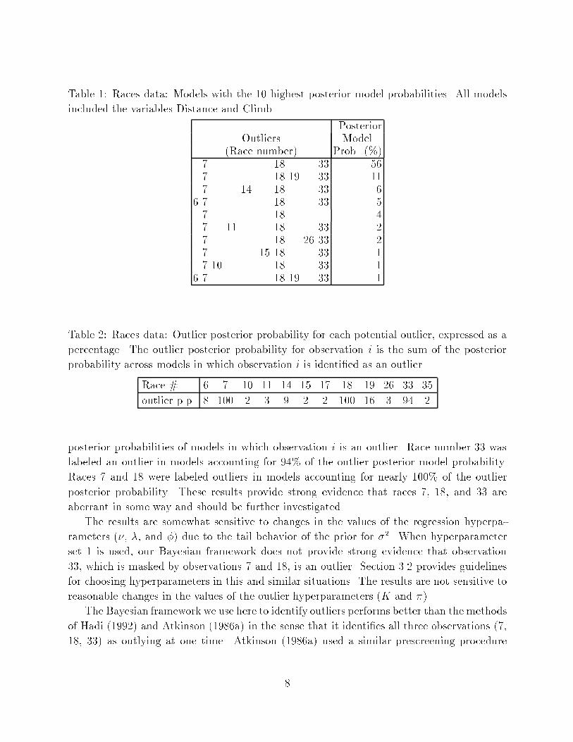
Table 1: Races data: Models with the 10 highest posterior model probabilities. All models
included the variables Distance and Climb.
PosteriorOutliers Model
(Race number) Prob. (%)7 18 33 567 18 19 33 117 14 18 33 6
6 7 18 33 57 18 47 11 18 33 27 18 26 33 27 15 18 33 17 10 18 33 1
6 7 18 19 33 1
Table 2: Races data: Outlier posterior probability for each potential outlier, expressed as a
percentage. The outlier posterior probability for observation i is the sum of the posterior
probability across models in which observation i is identi�ed as an outlier.
Race # 6 7 10 11 14 15 17 18 19 26 33 35
outlier p.p. 8 100 2 3 9 2 2 100 16 3 94 2
posterior probabilities of models in which observation i is an outlier. Race number 33 was
labeled an outlier in models accounting for 94% of the outlier posterior model probability.
Races 7 and 18 were labeled outliers in models accounting for nearly 100% of the outlier
posterior probability. These results provide strong evidence that races 7, 18, and 33 are
aberrant in some way and should be further investigated.
The results are somewhat sensitive to changes in the values of the regression hyperpa-
rameters (�, �, and �) due to the tail behavior of the prior for �2. When hyperparameter
set 1 is used, our Bayesian framework does not provide strong evidence that observation
33, which is masked by observations 7 and 18, is an outlier. Section 3.2 provides guidelines
for choosing hyperparameters in this and similar situations. The results are not sensitive to
reasonable changes in the values of the outlier hyperparameters (K and �).
The Bayesian framework we use here to identify outliers performs better than the methods
of Hadi (1992) and Atkinson (1986a) in the sense that it identi�es all three observations (7,
18, 33) as outlying at one time. Atkinson (1986a) used a similar prescreening procedure
8
to identify potential outliers, but his method identi�es observations 7 and 18 as outliers
in a second pass over the data before a third pass where he identi�es the masked outlier,
observation 33.
In conclusion, both race and climb are important predictors of record time for Scottish
Hill races. There is strong evidence that races 7, 18, and 33 are outlying. With a total
climb of 7500 feet, race number 7 has the largest total elevation gain of any race. Similarly,
race number 33 has the second longest climb of any race and is the third longest race. In a
more recent analysis of these data, Atkinson (1988) reports that the time for race number
18 is incorrect. An anonymous referee noted that the correct time for race 18 should be 16
minutes, 7 seconds as reported to him by Geo� Cohen of the University of Edinburgh. The
original data were used here so that results could be compared with the results of Hadi and
Atkinson.
4.2 Stack Loss
The stack loss data (Brownlee 1965) consist of 21 days of operation from a plant for the
oxidation of ammonia as a stage in the production of nitric acid. The response is called
\stack loss" which is the percent of unconverted ammonia that escapes from the plant.
There are three explanatory variables (Figure 2). The following description of the data is
given by Atkinson (1985, pg. 130):
The air ow [X1] measures the rate of operation of the plant. The nitric ox-
ides produced are absorbed in a counter-current absorption tower: X2 is the
inlet temperature of cooling water circulating through coils in this tower and X3
is proportional to the concentration of acid in the tower. Small values of the
response correspond to e�cient absorption of the nitric oxides.
The stack loss data have been considered by many authors including Daniel and Wood
(1980) and Atkinson (1985). The general consensus is that predictor X3 (acid concentration)
should be dropped from the model and that observations 1, 3, 4, and 21 are outliers. Single
deletion diagnostics for all 21 observations for the model with predictors X1, X2, and X3
provide little evidence for the presence of outliers, but robust analyses typically identify
these masked outliers.
Below, we consider outlier identi�cation and variable selection for the stack loss data.
Transformations are not considered in our analysis; however, there is some evidence that
inclusion of a quadratic term (x21) or an interaction term (x1x2) will lead to a better �tting
model (Figure 2). In addition, some authors have suggested that transformation of the
response may be appropriate (e.g., Atkinson 1985, and Chambers and Heathcote 1981).
Daniel and Wood (1980) explore the possibility of a temporal relationship in the data. We
have chosen not to further explore these issues in this paper.
9

Stack Loss
50 60 70 80
•••
•
••••••••
••••
• •
•••
•
• • ••••• • •
•• • •
•
75 80 85 90
•• •
•
• •••• ••• •
••• ••
• •
•••
•
••••••••
••••
• •
1000 1600 2200
1020
3040
•••
•
•••••••••
••••
• •
5060
7080 ••
•
•••••••••
••••
•
•
Air Flow
••
•• • •••• • •
• • •
•
•
•••
• ••• ••• •
••• ••
•
•
••
••
•
•
•
••
•••••••••
•••
•
•
••
••
••••
•
••
••
•••• •
•
••
•••
•
••••
••• • •
Watertemperature
••
••
••
••
• ••
••
••• •
• • •
•
••
•••
•
••••
••• • •
1822
26
•
••
•••
•
••••
••• • •
7580
8590 ••
•••
••
•
•
••
•
•
••
•
•••
•••
••
•
•
•
••
•
•
••
•
•••
•••
••• •
•
•
•
••
•
•
••
•
• ••
•
AcidConcentration
•••
•
•
•
•
••
•
•
••
•
•••
•••
••••
•
•
•
••
•
•
••
•
•••
•
••
•
•••••••••
•••••
•
•
•
••
••
•
•
•
•• • •••• • •
• • ••
•
••
•
• ••• ••• •
••• •••
•Air Flow xAir Flow
3000
5000
•
•
•••••••••
••••
•
10 20 30 40
1000
1600
2200 ••
•
•••••
•
••••••••
•
•
•
•
••••
•
••••
•••
•
•
18 22 26
•
•
•• • •
•
•• • •• • •
•
•
••
•
•••
••
• ••• •••• ••
•
•
3000 5000
•
•
••••
•
••••
•••
•
•Air Flow x
Watertemperature
Figure 2: Scatter plots of stack loss data.
10

Table 3: Stack loss data: Models with the 10 highest posterior model probabilities.
PosteriorOutliers Model
Predictors (Obs. number) Prob. (%)X1 X2 1 3 4 21 23X1 4 21 17X1 X2 4 21 9X1 X2 1 3 4 13 21 4X1 X2 21 3X1 21 3X1 X2 1 2 3 4 21 3X1 1 3 4 21 3X1 4 13 21 3X1 X2 3 4 21 2
For these data, the R2 for the full model is 0.91. As this is a high value of R2, we again
used hyperparameter set 2 for this analysis. We chose � = 0:1 and K = 7.
We used the prescreening method described in Section 3.3 to identify potential outliers.
This method indicated that 9 of the 21 observations (observations 1, 2, 3, 4, 8, 13, 14, 20,
21) were potential outliers. Using the set of potential outliers identi�ed by the prescreening
procedure, we calculated the posterior model probabilities for all possible combinations of
variables and outliers.
The models with the 10 highest posterior model probabilities are shown in Table 3.
The model with the highest posterior model probability includes predictors X1 and X2, and
outliers 1, 3, 4, and 21. Thus the model with the highest posterior model probability includes
the four masked outliers.
The posterior probability that the coe�cient for each predictor does not equal 0, i.e.,
Pr(�i 6= 0jD), is obtained by summing the posterior probabilities across models containing
each predictor. Air ow to the plant, X1, and cooling water temperature, X2, both received
support from the data with Pr(�i 6= 0jD) = 1 and 0.62 respectively, while acid concentration,
X3, did not with Pr(�3 6= 0jD) = 0:06.
The marginal posterior distributions for the coe�cients of the predictors for the stack
loss data are shown in Figure 3. The posterior distribution for the coe�cient for air ow (�1)
is centered away from 0. The posterior �1 has two modes showing that there is considerable
uncertainty about the value of this coe�cient. The posterior distribution of the coe�cient
for water temperature (�2) is also centered away from 0. This posterior distribution includes
a spike at 0 corresponding to Pr(�i = 0jD) = 0:38. The coe�cient for acid concentration
(�3) is centered very near 0, with a large spike at 0 corresponding to Pr(�i = 0jD) = 0:94.
11

0.00.2
0.40.6
0.81.0
1.2
0 1 2 3 4 5 6
P(β1|D)
β1
0.0 0.2 0.4 0.6 0.8 1.0
P(β1= 0|D)
0.00.2
0.40.6
0.81.0
1.2
0 2 4 6 8 10 12
0.00.2
0.40.6
0.81.0
1.2
0 2 4 6 8 10 12
P(β2|D)
β2
0.0 0.1 0.2 0.3 0.4 0.5
P(β2= 0|D)
-0.20-0.15
-0.10-0.05
0.00.05
0.10
0 5 10 15 20
P(β3|D)
β3
0.0 0.2 0.4 0.6 0.8 1.0
P(β3= 0|D)
Figu
re3:
Themargin
alposterior
density
for�1 ,�2 ,and�3of
thestack
lossdata
set.The
posterior
for�j ,pr(�
j jD),isan
averageacross
allmodels.
Thespikeat
0corresp
ondsto
pr(�
j=0jD
).Thevertical
axison
theleft
correspondsto
theposterior
distrib
ution
for�i
andthevertical
axison
therigh
tcorresp
ondsto
theposterior
distrib
ution
for�iequalto
0.
12

5 Bayesian Model Averaging Via Simultaneous Vari-
able Selection and Outlier Identi�cation
A typical approach to data analysis is to carry out a model selection exercise leading to
a single \best" model and to then make inferences as if the selected model were the true
model. However, this ignores a major component of uncertainty, namely uncertainty about
the model itself (Leamer 1978, Raftery 1993, Draper 1995). As a consequence, uncertainty
about quantities of interest can be underestimated. For striking examples of this see Regal
and Hook (1991) and Kass and Raftery (1995).
Below we address the problem of model uncertainty and suggest a method for accounting
for this uncertainty using Bayesian model averaging. We brie y summarize Bayesian model
averaging and describe MC3. We also discuss several methods for assessing predictive per-
formance. Finally, we provide an example that shows that that model averaging via SVO
improves predictive performance as compared with any single model that might reasonably
be selected.
5.1 Accounting for Model Uncertainty Via BMA
The standard Bayesian solution to the problem of model uncertainty involves averaging over
all possible models. If M = fM1; : : : ;MLg denotes the set of all models being considered
and if � is the quantity of interest such as a future observation or the utility of a course of
action, then the posterior distribution of � given the data D is
pr(� j D) =LX`=1
pr(� jM`;D)pr(M` j D); (2)
(Leamer 1978, p.117). This is an average of the posterior distribution under each model
weighted by the corresponding posterior model probabilities. We call this \Bayesian model
averaging" (BMA). For further details on BMA as applied to linear regression models see
Raftery et al. (1994).
Implementation of BMA is di�cult for two reasons. First, integrals used to compute
pr(M`jD) can be di�cult to solve. Second, the number of terms in (2) can be enormous.
Our Bayesian set-up described in Section 3 solves the �rst problem. The MC3 procedure
described below solves the second problem producing an estimate of the Bayesian model
average for the entire model space. An alternative method, called Occam's Window, can be
used to select models to include in the Bayesian model average (Raftery et al. 1994).
5.2 Markov Chain Monte Carlo Model Composition
For some problems, the number of possible models is very large and it becomes too compu-
tationally intensive to compute the posterior probability for every model. To address this
13
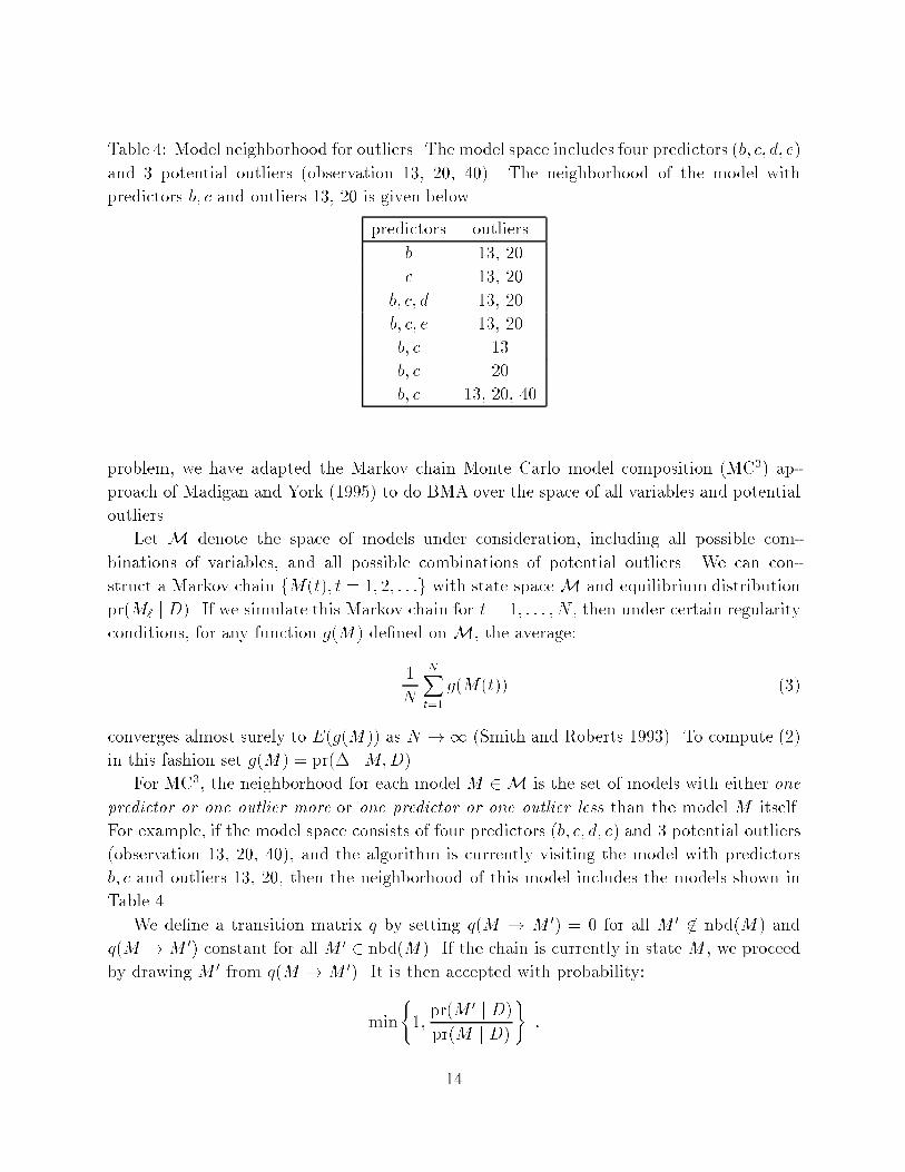
Table 4: Model neighborhood for outliers. The model space includes four predictors (b; c; d; e)
and 3 potential outliers (observation 13, 20, 40). The neighborhood of the model with
predictors b; c and outliers 13, 20 is given below.
predictors outliers
b 13, 20
c 13, 20
b; c; d 13, 20
b; c; e 13, 20
b; c 13
b; c 20
b; c 13, 20, 40
problem, we have adapted the Markov chain Monte Carlo model composition (MC3) ap-
proach of Madigan and York (1995) to do BMA over the space of all variables and potential
outliers.
Let M denote the space of models under consideration, including all possible com-
binations of variables, and all possible combinations of potential outliers. We can con-
struct a Markov chain fM(t); t = 1; 2; : : :g with state spaceM and equilibrium distribution
pr(M` j D). If we simulate this Markov chain for t = 1; : : : ; N , then under certain regularity
conditions, for any function g(M) de�ned on M, the average:
1
N
NXt=1
g(M(t)) (3)
converges almost surely to E(g(M)) as N !1 (Smith and Roberts 1993). To compute (2)
in this fashion set g(M) = pr(� jM;D).
For MC3, the neighborhood for each model M 2 M is the set of models with either one
predictor or one outlier more or one predictor or one outlier less than the model M itself.
For example, if the model space consists of four predictors (b; c; d; e) and 3 potential outliers
(observation 13, 20, 40), and the algorithm is currently visiting the model with predictors
b; c and outliers 13, 20, then the neighborhood of this model includes the models shown in
Table 4.
We de�ne a transition matrix q by setting q(M ! M 0) = 0 for all M 0 62 nbd(M) and
q(M !M 0) constant for all M 0 2 nbd(M). If the chain is currently in state M , we proceed
by drawing M 0 from q(M !M 0). It is then accepted with probability:
min
(1;pr(M 0 j D)
pr(M j D)
):
14

Otherwise the chain stays in state M .
Software for implementing the MC3 algorithm is described in the Appendix.
5.3 Assessment of Predictive Performance
A primary purpose of statistical analysis is to make forecasts for the future. For MC3, our
speci�c objective is to compare the quality of the predictions from model averaging with the
quality of predictions from any single model that an analyst might reasonably have selected.
To measure performance we randomly split the complete data into two subsets. We run
MC3 using one portion of the data. We call this the training set, DT . We used the remaining
portion of the data to assess performance, calling this the prediction set where DP = DnDT .
The two measures of performance we use are based on the posterior predictive distri-
bution, described below. The �rst measure of predictive ability is the coverage for 90%
prediction intervals. Predictive coverage was measured using the proportion of observations
in the performance set that fall in the corresponding 90% posterior prediction interval.
The second measure of predictive ability is the logarithmic scoring rule of Good (1952)
where for each event A which occurs, a score of � log fpr(A)g is assigned. The log predictive
score is based on the posterior predictive distribution suggested by Geisser (1980). In this
paper, we compare the log predictive score of individual models to the log predictive score
of BMA via MC3. A small log predictive score indicates a model predicts observations in
the prediction set well. In this See Raftery et al. (1994) for details on the computation of
predictive coverage and the log predictive score.
We denote the posterior predictive distribution by pr(wjy), where w is an observation in
the prediction set and y is the vector of observations from the training set. To accommodate
the possibility that an observation in the prediction set might be an outlier, we adopt a
mixture distribution for the posterior predictive distribution:
pr(w j y) = �p0(w j y) + (1 � �)p1(w j y) (4)
where p0 is the posterior predictive distribution when w is an outlier and p1 is the posterior
predictive distribution when w is not an outlier.
To assess predictive performance, we incorporate information gleaned from the training
set about the prevalence of outliers in the data. To this end, we calculate an updated value
of the proportion of outliers, �̂ =PL
`=1 pr (M` j D) q`=nT , where L is the number of models,
pr (M` j D) is the posterior model probability for model `, q` is the number of observations
identi�ed as outliers under model `, and nT is the number of observations in the training
set. To compute the posterior predictive distribution in equation (4), we use the maximum
of the original value of � used for the training set run, and �̂. This ensures the possibility
of detecting outliers in the prediction set even if there are no outliers in the training data.
Experience to date indicates that for di�erent random splits of the same data set, the
algorithms often select di�erent models, but that the log predictive scores for BMA tend to
15

be similar across the random splits.
In the example that follows, we explore how accounting for uncertainty in variable selec-
tion and outlier identi�cation in uences predictive performance.
5.4 Example: Liver Surgery
A hospital surgical unit interested in predicting survival in patients undergoing a particular
type of liver operation collected data on a sample of 108 patients (Neter, Wasserman, and
Kutner 1990, henceforth referred to as NWK). Four predictors were extracted from records
of the preoperation evaluation of each patient:
X1 blood clotting score
X2 prognostic index, which includes the age of patient
X3 enzyme function test score
X4 liver function test score
The response is patient survival time. We used 54 patients for model building and the other
54 patients to assess predictive ability. NWK use the same split of the data for similar
purposes. Figure 4 shows a scatterplot matrix for the entire data.
As in NWK we transformed the response logarithmically, so Y 0 = log10Y . Both forms
of the response are shown in Figure 4. After transforming the response, standard diagnos-
tic checking (e.g., Weisberg 1985) does not reveal any gross violations of the assumptions
underlying normal linear regression.
To demonstrate MC3 on a data set with known outliers, we introduced arti�cial outliers
in the liver surgery data. To generate outliers we multiplied the �rst �ve responses in the
training set and the last two responses in the prediction set by 2 before logarithmically
transforming the response. We will call these seven observations the \simulated outliers."
While multiplying the response by 2 amounts to a shift in mean, we are using a variance-
in ation model to accommodate outliers. However, by increasing the values of these 5
observations, we are, in e�ect, increasing the variance as well. The goal of this exercise is to
determine whether our method correctly identi�es these aberrant observations.
For the training set, diagnostic plots of the residuals indicate that the simulated outliers
(observations 1{5) are quite di�erent from the rest of the observations (Figure 5). The
absolute values of Studentized residuals for the �ve simulated outliers range from 2.4 to 3.0
while the Studentized residuals for the rest of the data set range from -1.7 to 1.4. However,
Weisberg's outlier test (1985), which is based on the Studentized residuals, does not indicate
that these observations are outlying. So while visual inspection of the diagnostic plots might
lead to the conclusion that the simulated observations are outlying, there is some uncertainty
about whether or not this is the case.
The prescreening procedure identi�ed 18 potential outliers in the training set. They
are observations 1, 2, 3, 4, 5, 9, 15, 19, 22, 27, 28, 30, 37, 38, 39, 43, 46, and 54. These
16

survivaltime
1.5 2.0 2.5
•
•
•
•
•
••
•••
•
•
•
••
••
••• •
•
••
• •
•
•
•
•••
•
••
•• ••••
•
• ••
••
•
•
••
•
•
••
• • •••
• •••
••
•
••
•
•
•
•
•
•
•
••••
•
•
•
•
••
••
•
••
•
•
•
••
••
•
•
•
•••• •
•
•
•
•
•
•••
•••
•
•
•
••
••
••••
•
••
••
•
•
•
• ••
•
••
• • • •••
•
•••
••
•
•
•••
•
•
••
•••
•••••
•
••
•
••
•
•
•
•
•
•
•
••••
•
•
•
•
••
••
•
••
•
•
•
••
• •
•
•
•
•• •••
20 60 100
•
•
•
•
•
• ••• •
•
•
•
•
••
••
••• •
•
••
••
•
•
•
•••
•
••
•• ••••
•
• ••
••
•
•
• ••
•
•
••
• ••• •
• •••
••
•
•••
•
•
•
•
•
•
• •••
•
•
•
•
••
••
•
••
•
•
•
••
••
•
•
•
•• •• •
•
•
•
•
•
•••
•••
•
•
•
••
••
• •••
•
••
• •
•
•
•
•••
•
••
• •• •• •
•
• ••
••
•
•
•••
•
•
••
•••
•••• •
•
••
•
••
•
•
•
•
•
•
•
•••••
•
•
•
• •
••
•
••
•
•
•
••••
•
•
•
• ••••
1 2 3 4 5 6
510
15
•
•
•
•
•
• ••••
•
•
•
•
••
••
••••
•
••
••
•
•
•
• ••
•
••
• •••••
•
•••
••
•
•
•••
•
•
••
•••
• •• • •
•
••
•
••
•
•
•
•
•
•
•
• ••••
•
•
•
••
••
•
••
•
•
•
••
••
•
•
•
•• •••
1.5
2.0
2.5
•
•
•
•
•
••
•••
•
•
•
••
•
•
••• •
•
• •
• •
•
•
•
••
•
•
••
•• ••••
•
• ••
• •
•
•
••
•
•
••
•••
••
• •••
••
•
•
••
•
•
•
•
••
••••
•
•
•
•
•
••
•
•
•
•
•
•
••
••
•
•
•
••••
• survivaltime
(log10)
•
•
•
•
•
•••
•••
•
•
•
••
•
•
••••
•
• •
••
•
•
•
• •
•
•
••
• • • •••
•
•••
••
•
•
•••
•
•
••
•••
••
••••
••
•
•
••
•
•
•
•
••
••••
•
•
•
•
••
• •
•
•
•
•
•
•
••
••
•
•
•
•• ••
••
•
•
•
•
• ••• •
•
•
•
•
••
•
•
••• •
•
••
••
•
•
•
••
•
•
••
•• ••••
•
• ••
• •
•
•
• ••
•
•
••
• ••
• •
• •••
••
•
•
••
•
•
•
•
••
• •••
•
•
•
•
••
••
•
•
•
•
•
•
••
••
•
•
•
•• ••
••
•
•
•
•
•••
•••
•
•
•
••
•
•
• •••
•
• •
• •
•
•
•
••
•
•
••
• •• •• •
•
• ••
••
•
•
•••
•
•
••
•••
••
•• ••
••
•
•
••
•
•
•
•
••
•••••
•
•
•
• •
••
•
•
•
•
•
•
•••
•
•
•
•
• ••••
•
•
•
•
•
• ••••
•
•
•
•
••
•
•
••••
•
••
••
•
•
•
• •
•
•
••
• •••••
•
•••
• •
•
•
•••
•
•
••
•••
• •
• • ••
••
•
•
••
•
•
•
•
••
• ••••
•
•
•
••
••
•
•
•
•
•
•
••
••
•
•
•
•• ••
•
•
•
••
•
••
•
•
•
••••
• ••
•
•
••
•
•• ••
•
•
••
•
•
••• •
•
• •••
•
•
•
•
•
• •••
•• •
•
•
•
•••
••
•
• •••
• • ••
•
•
•
•
•••
••
•
••• •
• •
•••
••
••
•
•
•••
•
• ••
•
••
••
•
•
•
••
•
••
•
•
•
••••
• ••
•
•
••
•
•• ••
•
•
••
•
•
••• •
•
• •••
•
•
•
•
•
• •••
•• •
•
•
•
•• •
••
•
• •••
• • ••
•
•
•
•
•••
••
•
••• •
• •
•••
••
••
•
•
•••
•
• ••
•
••
••
•
bloodclottingscore
•
•
••
•
• •
•
•
•
••••
• ••
•
•
••
•
••••
•
•
••
•
•
••••
•
• •••
•
•
•
•
•
• •••
• ••
•
•
•
•• •
••
•
• •••
•• ••
•
•
•
•
•••
••
•
••• •
• •
••••
••
•
•
•
•••
•
• ••
•
••
••
•
•
•
••
•
••
•
•
•
••••
•••
•
•
••
•
•• •••
•
••
•
•
••• •
•
••••
•
•
•
•
•
•••
•
•• •
•
•
•
•••
••
•
•• ••
• • ••
•
•
•
•
•••
••
•
••• •
• •
• ••
••
••
•
•
••••
• ••
•
• •
••
• 46
810
•
•
••
•
• •
•
•
•
•••
•••
•
•
••
•
••• •
•
•
••
•
•
••••
•
••••
•
•
•
•
•
• •••
•• •
•
•
•
•••
••
•
• • ••
• • ••
•
•
•
•
••••
•
•
•• ••
• •
••••
••
•
•
•
•••
•
• ••
•
••
••
•
2060
100
•• •
••
••
• ••
•
•
••
••
•
•
•••
•
•
•••
•
•
•
••
••
••
•
•
•
•••
•
•
•
•
•
••
•••
•
•
•
•
•
•
•••
•
•
•
•
••• •
•
•• •
•
•
•••
••
•
••
•
•
•
•
••
••
•
•••
•
•• ••
•
•
• •••
•
•
• •• •
••
••
• ••
•
•
••
••
•
•
•••
•
•
•••
•
•
•
••
••
••
•
•
•
•••
•
•
•
•
•
••
•••
•
•
•
•
•
•
•••
•
•
•
•
••• •
•
•• •
•
•
•••
••
•
••
•
•
•
•
••
••
•
•••
•
•• ••
•
•
• •••
•
•
• •• •
••
••
• ••
•
•
••
••
•
•
•••
•
•
•••
•
•
•
••
••
•••
•
•
•••
•
•
•
•
•
••
•• •
•
•
•
•
•
•
••
••
•
•
•
•• ••
•
•••
•
•
•••
••
•
••
•
•
•
•
••
• •
•
•••
•
•• ••
•
•
• •••
•
•
•
prognosticindex
•• •
••
••
• ••
•
•
••
••
•
•
•••
•
•
•••
•
•
•
••
••
••
•
•
•
•••
•
•
•
•
•
••
•••
•
•
•
•
•
•
••
••
•
•
•
••• •
•
•• •
•
•
•••
••
•
••
•
•
•
•
• •
••
•
•••
•
•• ••
•
•
• •• •
•
•
• •• •
••
••
•••
•
•
••
••
•
•
•••
•
•
•• •
•
•
•
••
•••
••
•
•
•••
•
•
•
•
•
••
•••
•
•
•
•
•
•
••
••
•
•
•
••• •
•
•••
•
•
•••
••
•
••
•
•
•
•
••
••
•
•••
•
•• ••
•
•
• •••
•
•
•
••
•
•
•
••
•••
•
•
•
•
• •
••
••
•
••
••
•• •
• ••
•
•
•
•
••
•
••
•
••
••
•
• •
•
•
••
•••
•
•
•••
••
• ••
•
•
•
•••
• •
•
•
•
••
•
•
••••
•
•
••
•
•
•
••
••
•
•••
•
•
••
••
•
• •
••
•
•
•
••
•••
•
•
•
•
• •
••
••
•
••
••
•• •
• ••
•
•
•
•
••
•
••
•
••
••
•
• •
•
•
••
•••
•
•
• ••
••
• ••
•
•
•
•••
• •
•
•
•
••
•
•
••••
•
•
••
•
•
•
••
••
•
•••
•
•
••
••
•
• •
••
•
•
•
••
••••
•
•
•
••
••
••
•
••
••
•• •
• ••
•
•
•
•
••
•
•••
••
••
•
••
•
•
••
•••
•
•
•••
••
•••
•
•
•
•••
• •
•
•
•
••
•
•
••••
•
•
••
•
•
•
••
••
•
••••
•
••
••
•
••
•••
•
•
••
•• •
•
•
•
•
• •
••
••
•
••
••
•• •
• ••
•
•
•
•
••
•
••
•
••
••
•
• •
•
•
• •
•••
•
•
• ••
••
• ••
•
•
•
•••
• •
•
•
•
••
•
•
••••
•
•
••
•
•
•
••
••
•
•••
•
•
••
••
•
• • enzymefunction
2060
100
••
•
•
•
••
•••
•
•
•
•
••
••
•••
••
••
•• •
•••
•
•
•
•
••
•
•••
••
••
•
• •
•
•
••
••••
•
•••
••
• •••
•
•
•••
• •
•
•
•
••
•
•
•• ••
•
•
••
•
•
•
••
••
•
•••
•
•
••
••
•
••
5 10 15
12
34
56
••
••
•
••
• ••
•
•
•••
••
•
•••
••
••
•
•
•
• •
•
•• •• ••• •••
•
•
•
•
• •
•
•
•
••
••
•
•
•
••••• •
•• •
••
•
••
•••
••
••
••
•
•
• •
•
••
•
••
•
••
•
•
••
•
•
•
•
•
•
•
•
•• ••
•••
•
••
• ••
•
•
•••
••
•
•••
••
••
•
•
•
• •
•
•• •• ••• •••
•
•
•
•
• •
•
•
•
••
••
•
•
•
• • ••• •
•• •
••
•
••
•••
••
••
••
•
•
• •
•
••
•
••
•
••
•
•
••
•
•
•
•
•
•
•
•
•• •
4 6 8 10
••
••
•
••
• ••
•
•
••
••
•
•••
••
••
•
•
•
• •
•
•• •••
•• •
•••
•
•
•
••
•
•
•
••
••
•
•
•
•• ••
• •
•••
••
•
••
•••
••
• •
••
•
•
••
•
••
•
• •
•
••
•
•
••
•
•
•
•
•
•
•
•
• •••
•• •
•
••
•• •
•
•
•••
••
•
•••
••
•••
•
•
• •
•
•• •••
•• •
•••
•
•
•
• •
•
•
•
••
••
•
•
•
• •••
••
•• •
••
•
•••
••
••
••
••
•
•
• •
•
••
•
••
•
••
•
•
••
•
•
•
•
•
•
•
•
•• •
20 60 100
••
••
•
••
• ••
•
•
••••
•
•
•••
••
••
•
•
•
••
•
•• •• •
•••
•••
•
•
•
• •
•
•
•
••
••
•
•
•
•• ••
• •
• • •
••
•
••
•••
••
••
••
•
•
• •
•
••
•
••
•
••
•
•
••
•
•
•
•
•
•
•
•
• ••
liverfunction
Figure 4: Scatter plots of the entire liver surgery data without outliers added.
17

Quantiles of Standard Normal
stud
entiz
ed r
esid
uals
-2 -1 0 1 2
-10
12
3
•
•••
•
•
••
•
•
•
•••
••
••
•
••••
••
•
•
•
•
•
••
•
••
•
1 2
3
4
5
Quantile-Quantile Plot of Studentized Residuals
fitted values
stud
entiz
ed r
esid
uals
1.6 1.8 2.0 2.2 2.4 2.6 2.8
-10
12
3
•
• ••
•
•
••
•
•
•
•••
••
••
•
• • ••
••
•
•
•
•
•
••
•
••
•
12
3
4
5
Fitted values versus Studentized Residuals
blood clotting score
stud
entiz
ed r
esid
uals
4 6 8 10
-10
12
3
•
•••
•
•
••
•
•
•
•••
••
••
•
•• ••••
•
•
•
•
•
••
•
•••
12
3
4
5
Blood Clotting Score versus Studentized Residuals
prognostic index
stud
entiz
ed r
esid
uals
20 40 60 80
-10
12
3
•
• ••
•
•
••
•
•
•
••••
•
••
•
• • ••
••
•
•
•
•
•
••
•
••
•
12
3
4
5
Prognostic Index versus Studentized Residuals
enzyme function
stud
entiz
ed r
esid
uals
20 40 60 80 100 120
-10
12
3
•
• ••
•
•
••
•
•
•
••••
•
••
•
• • ••
••
•
•
•
•
•
••
•
••
•
12
3
4
5
Enzyme Function versus Studentized Residuals
liver function
stud
entiz
ed r
esid
uals
1 2 3 4 5 6
-10
12
3
•
• ••
•
•
••
•
•
•
••••
•
••
•
• ••••
••
•
•
•
•
••
•
••
•
12
3
4
5
Liver Function versus Studentized Residuals
Figure 5: Residual plots of the liver surgery data for the training set (with outliers added).
Observations 1{5 are denoted by numbers and the 13 other observations in the set of potential
outliers (observation number 9, 15, 19, 22, 27, 28, 30, 37, 38, 39, 43, 46, 54) are denoted by
a � symbol.
18

Table 5: Liver surgery data with simulated outliers: MC3. For the log predictive score,
�̂ = 0:07. Predictive Coverage % is the percentage of observations in the performance set
that fall in the 90% prediction interval.
Posterior Log PredictiveOutliers Model Predictive Coverage
Predictors (Obs. number) Prob. (%) Score %MC3
X1 X2 X3 1 2 3 4 5 50 25.0 80X1 X2 X3 none 10 14.0 96X1 X2 X3 1 2 3 4 5 22 5 32.6 72X1 X2 X3 X4 1 2 3 4 5 4 24.9 80X1 X2 X3 1 2 3 4 3 20.9 85X1 X2 X3 X4 none 2 15.1 96X1 X2 X3 4 2 15.2 96X1 X2 X3 2 2 14.0 96X1 X2 X3 1 1 13.2 96X1 X2 X3 1 2 4 1 17.8 91MC3 model averaging 19.4 89
observations are denoted by the � symbol in Figure 5. Note that the simulated outliers were
all identi�ed as potential outliers by the prescreening procedure.
Since R2 < 0:9, we used hyperparameter set 1, K = 7, and � = 0:02. All possible models
(i.e., all possible combinations of variables and outliers) were assumed to be equally likely a
priori. In total, 184 models were visited in 20,000 iterations of MC3. The models with the 10
highest posterior probabilities are shown in Table 5. The model with the highest posterior
model probability includes the predictors X1, X2, X3 and the 5 simulated outliers.
The probabilities that the coe�cients for each predictor do not equal 0, Pr(�i 6= 0jD),
are .91, .91, .91, and .09, respectively. Thus there is little support for inclusion of the
predictor liver function test score (X4) in the model. NWK also conclude that this is not
a useful predictor. The outlier posterior probability for each potential outlier in given in
Table 6. The simulated outliers (observations 1{5) were identi�ed as outliers in over 70% of
the models.
Based on the training set, the estimated value for �̂ (used in the calculation of prediction
coverage and log predictive score for outliers) was 0.07 for MC3.
Predictive coverage is given in Table 5. The individual models tend to overstate or
understate the predictive coverage. Compared to the individual models, model averaging
produces more accurate prediction coverage.
19
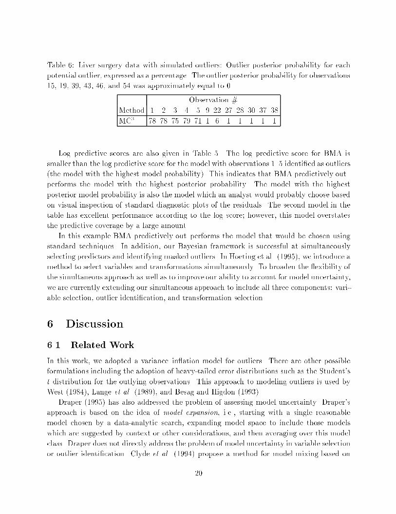
Table 6: Liver surgery data with simulated outliers: Outlier posterior probability for each
potential outlier, expressed as a percentage. The outlier posterior probability for observations
15, 19, 39, 43, 46, and 54 was approximately equal to 0.
Observation #
Method 1 2 3 4 5 9 22 27 28 30 37 38
MC3 78 78 75 79 71 1 6 1 1 1 1 1
Log predictive scores are also given in Table 5. The log predictive score for BMA is
smaller than the log predictive score for the model with observations 1{5 identi�ed as outliers
(the model with the highest model probability). This indicates that BMA predictively out{
performs the model with the highest posterior probability. The model with the highest
posterior model probability is also the model which an analyst would probably choose based
on visual inspection of standard diagnostic plots of the residuals. The second model in the
table has excellent performance according to the log score; however, this model overstates
the predictive coverage by a large amount.
In this example BMA predictively out{performs the model that would be chosen using
standard techniques. In addition, our Bayesian framework is successful at simultaneously
selecting predictors and identifying masked outliers. In Hoeting et al. (1995), we introduce a
method to select variables and transformations simultaneously. To broaden the exibility of
the simultaneous approach as well as to improve our ability to account for model uncertainty,
we are currently extending our simultaneous approach to include all three components: vari-
able selection, outlier identi�cation, and transformation selection.
6 Discussion
6.1 Related Work
In this work, we adopted a variance{in ation model for outliers. There are other possible
formulations including the adoption of heavy-tailed error distributions such as the Student's
t distribution for the outlying observations. This approach to modeling outliers is used by
West (1984), Lange et al. (1989), and Besag and Higdon (1993).
Draper (1995) has also addressed the problem of assessing model uncertainty. Draper's
approach is based on the idea of model expansion, i.e., starting with a single reasonable
model chosen by a data-analytic search, expanding model space to include those models
which are suggested by context or other considerations, and then averaging over this model
class. Draper does not directly address the problem of model uncertainty in variable selection
or outlier identi�cation. Clyde et al. (1994) propose a method for model mixing based on
20

a reexpression of the space of models in terms of an orthogonalization of the design matrix.
George and McCulloch (1993) developed the Stochastic Search Variable Selection (SSVS)
method which is similar in spirit to MC3. In a more recent paper (1994), they suggest an
extension of their approach to simultaneous variable selection and outlier identi�cation.
6.2 Conclusions
In this paper we introduced a Bayesian approach to simultaneous variable selection and out-
lier identi�cation. SVO overcomes the problem that the model you select depends upon the
order in which you consider variable selection and outlier identi�cation. We also introduced
a method for the identi�cation of multiple outliers which appears to be successful in the
identi�cation of masked outliers. Finally, we demonstrated that the model averaging via
MC3 improves predictive performance.
In addition to variable selection and outlier identi�cation, there is also uncertainty in-
volved in the choice of transformations in regression.
A Software for Implementing MC3
BMA is a set of S-PLUS functions which can be obtained free of charge via the World Wide
Web address http://lib.stat.cmu.edu/S/bma or by sending an e-mail message containing
the text \send BMA from S" to the Internet address [email protected].
The program MC3.REG performs Markov chain Monte Carlo model composition for
linear regression allowing for simultaneous variable selection and outlier identi�cation. The
set of programs fully implements the MC3 algorithm described in Section 5.2.
References
References
[1] Adams, J. L. (1991). A computer experiment to evaluate regression strategies, Proceed-ings of the American Statistical Association Section on Statistical Computing, 55{62.
[2] Atkinson, A. C. (1985). Plots, Transformations, and Regression, Clarendon Press: Ox-ford.
[3] Atkinson, A. C. (1986a). Masking unmasked, Biometrika, 73, 533{541.
[4] Atkinson, A.C. (1986b). Comments on \In uential Observations, High Leverage Points,and Outliers in Linear Regression," Statistical Science, 1, 397{402.
[5] Atkinson, A. C., Transformations unmasked (1988). Technometrics, 30, 311{318.
21

[6] Barnett V. and T. Lewis (1994). Outliers in Statistical Data, 3rd edition, Wiley: NewYork.
[7] Besag, J. E. and D.M. Higdon (1993). Bayesian inference for agricultural �eld experi-ments, Bull. Int. Statist. Inst., 55, 121 { 136.
[8] Blettner, M. and W. Sauerbrei (1993). In uence of Model-Building Strategies on theresults of a Case-Control Study, Statistics in Medicine, 12, 1325{1388.
[9] Bloom�eld, P. and W.L. Steiger (1983). Least Absolute Deviations: Theory, Applica-
tions, and Algorithms, Birkh�auser: Boston.
[10] Box, G.E.P. and G.C. Tiao (1968). A Bayesian approach to some outlier problems,Biometrika, 55, 119{129.
[11] Brownlee, K. A. (1965). Statistical Theory and Methodology in Science and Engineering,2nd edition, Wiley: New York.
[12] Chambers, R. L. and C.R. Heathcote (1981). On the estimation of slope and identi�ca-tion of outliers in linear regression, Biometrika, 68, 21{33.
[13] Chatterjee, S. and A.S. Hadi (1986). In uential observations, high leverage points, andoutliers in linear regression, Statistical Science, 1, 379{416.
[14] Clyde, M., H. DeSimone, and G. Parmigiani (1996). Prediction via OrthogonalizedModel Mixing. Journal of the American Statistical Association, to appear.
[15] Daniel, C. and F.S. Wood (1980). Fitting Equations to Data, Wiley: New York.
[16] Draper, D. (1995). Assessment and Propagation of Model Uncertainty (with discussion),Journal of the Royal Statistical Society B, 57, 45{97.
[17] Garthwaite, P.H. and J.M. Dickey (1992). Elicitation of prior distributions for variable-selection problems in regression, Annals of Statistics, 20(4), 1697{1719.
[18] Geisser, S. (1980). Discussion on Sampling and Bayes' inference in scienti�c modelingand robustness (by G. E. P. Box), Journal of the Royal Statistical Society A, 143,416{417.
[19] George, E.I. and R.E. McCulloch (1993). Variable selection via Gibbs sampling, Journalof the American Statistical Association, 88(423), 881{890.
[20] George, E. I. and R.E. McCulloch (1994). Fast Bayes Variable Selection, CSS TechnicalReport 94-01, University of Texas at Austin.
[21] Good, I.J. (1952). Rational Decisions, Journal of the Royal Statistical Society B, 14,107{114.
22

[22] Guttman, I., R. Dutter, and P.R. Freeman (1978). Care and handling of univariateoutliers in the general linear model to detect spuriousity, Technometrics, 20, 187{193.
[23] Hadi, A.S. (1990). A stepwise procedure for identifying multiple outliers in linear regres-sion, American Statistical Association Proceedings of the Statistical Computing Section,137{142.
[24] Hadi, A.S. (1992). A new measure of overall potential in uence in linear regression,Computational Statistics and Data Analysis, 14, 1{27.
[25] Hawkins, D.M. (1980). Identi�cation of Outliers, Chapman and Hall: London.
[26] Heiberger, R. and R.A. Becker (1991). Design of an S function for Robust RegressionUsing Iteratively Reweighted Least Squares, AT&T Statistics Research Report.
[27] Hettmansperger, T.P. and S.J. Sheather (1992). A cautionary note on the method ofleast median squares, The American Statistician, 46, 79{83.
[28] Hoaglin, D.C., F. Mosteller and J.W. Tukey (1983). editors, Understanding Robust and
Exploratory Data Analysis, Wiley: New York.
[29] Hoeting, J.A. (1994). Accounting for Model Uncertainty in linear regression. Ph.D. dis-sertation, University of Washington. (See http://www.stat.colostate.edu).
[30] Hoeting, J., A.E. Raftery, D. Madigan, (1995). Simultaneous Variable and Transforma-tion Selection in Linear Regression, Technical Report 9506, Department of Statistics,Colorado State University.
[31] Kadane, J. B., Dickey, J. M., Winkler, R. L., Smith, W. S. and Peters,S. C. (1980).Interactive elicitation of opinion for a normal linear model, Journal of the American
Statistical Association, 75, 845{854.
[32] Kass, R.E. and A.E. Raftery (1995). Bayes Factors, Journal of the American Statistical
Association, 90, 773{795.
[33] Kianifard, F. and W.H. Swallow (1989). Using recursive residuals, calculated onadaptively-ordered observations, to identify outliers in linear regression, Biometrics,45, 571{585.
[34] Lange, K.L., R.J.A. Little, and J.M.G. Taylor (1989). Robust statistical modeling usingthet-distribution, Journal of the American Statistical Association, 84, 881-896.
[35] Leamer, E. (1978). Speci�cation Searches: Ad Hoc Inference with Nonexperimental Data,Wiley: New York.
[36] Madigan, D. and Raftery, A. E. (1994). Model selection and accounting for model uncer-tainty in graphical models using Occam's Window, Journal of the American Statistical
Association, 89, 1535-1546.
23

[37] Madigan, D. and York, J. (1995). Bayesian graphical models for discrete data, Interna-tional Statistical Review, 63(1995) 215-232.
[38] Marasinghe, M. G. (1985). A multistage procedure for detecting several outliers in linearregression, Technometrics, 27, 395{399.
[39] Neter, J., Wasserman, W., and Kutner, M. (1990). Applied Linear Statistical Models,Irwin: Homewood, IL.
[40] Pettit, L. I. (1992). Bayes Factors for outlier models using the device of imaginaryobservations, Journal of the American Statistical Association, 87, 541{545.
[41] Raftery, A. E. (1993a). Approximate Bayes factors and accounting for model uncertaintyin generalized linear models, Technical Report 255, Department of Statistics, Universityof Washington.
[42] Raftery, A. E., Madigan, D., and Hoeting, J. (1994). Bayesian Model Averaging forLinear Regression Models Technical Report 9412, Department of Statistics, ColoradoState University. (See http://www.stat.colostate.edu).
[43] Regal, R. and Hook, E. B. (1991). The e�ects of model selection on con�dence intervalsfor the size of a closed population, Statistics in Medicine, 10, 717{721.
[44] Rousseeuw, P. J. (1984). Least median of squares regression. Journal of the American
Statistical Association, 79, 871{88.
[45] Rousseeuw, P. J. and Leroy, A. M. (1987). Robust Regression and Outlier Detection,Wiley: New York.
[46] Smith, A. F. M. and Roberts, G. O. (1993). Bayesian computation via Gibbs samplerand related Markov chain Monte Carlo methods, Journal of the Royal Statistics SocietyB, 55, 3{24.
[47] Taplin, R. and Raftery, A. E. (1994). Analysis of agricultural �eld trials in the presenceof outliers and fertility jumps, Biometrics, 50, 764-781.
[48] Verdinelli, I. and Wasserman, L. (1991). Bayesian analysis of outlier problems using theGibbs sampler, Statistics and Computing, 1, 105-117.
[49] Weisberg, S. (1985). Applied Linear Regression, Wiley: New York.
[50] West, M. (1984). Outlier Models and Prior Distributions in Bayesian Linear Regression,Journal of the Royal Statistics Society B, 46, 431{439.
24


