2. Motion relationships and torques

167

Application GuidelinesCalculation data

Tech

nica

lAn

nex

Service Phone Europe

+ 49 (0 ) 71 42 / 353-0 Service Phone North America + 1 – 2 6 9 / 6 3 7 7 9 9 9

2. Motion relationships and torques

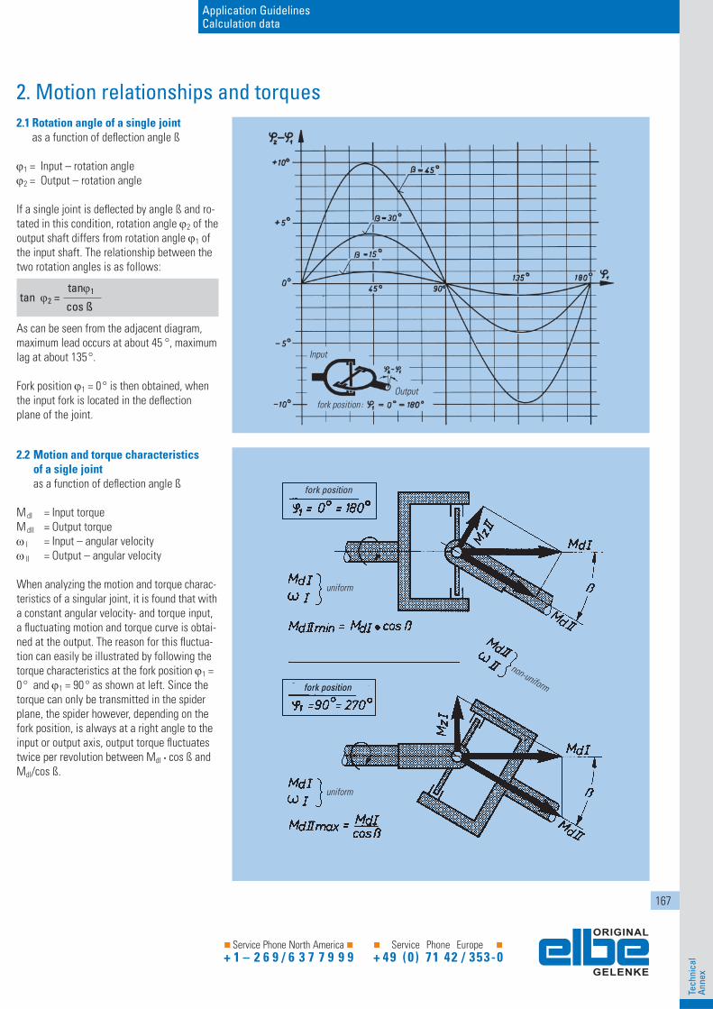
2.2 Motion and torque characteristics of a sigle joint as a function of defl ection angle ß

M dI = Input torqueM dII = Output torque I = Input – angular velocity Il = Output – angular velocity

When analyzing the motion and torque charac-teristics of a singular joint, it is found that with a constant angular velocity- and torque input, a fl uctuating motion and torque curve is obtai-ned at the output. The reason for this fl uctua-tion can easily be illustrated by following the torque characteristics at the fork position 1 = 0° and 1 = 90° as shown at left. Since the torque can only be transmitted in the spider plane, the spider however, depending on the fork position, is always at a right angle to the input or output axis, output torque fl uctuates twice per revolution between MdI · cos ß and MdI/cos ß.

2.1 Rotation angle of a single joint as a function of defl ection angle ß

1 = Input – rotation angle2 = Output – rotation angle

If a single joint is defl ected by angle ß and ro-tated in this condition, rotation angle 2 of the output shaft differs from rotation angle 1 of the input shaft. The relationship between the two rotation angles is as follows:

tan 2 = tan1

cos ß

As can be seen from the adjacent diagram, maximum lead occurs at about 45 °, maximum lag at about 135°.

Fork position 1 = 0° is then obtained, when the input fork is located in the defl ection plane of the joint.

Input

Outputfork position

uniform

uniform

non-uniform

fork position

fork position

168

Tech

nica

lAn

nex

Catalog Spare parts Drive-Shaft Calculation Installation and Maintenance www.elbe-group.com

MdII = cos ß1

MdI max cos ß2( )

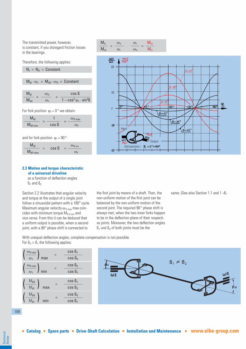
2.3 Motion and torque characteristic of a universal driveline as a function of defl ection angles ß1 and ß2

Section 2.2 illustrates that angular velocityand torque at the output of a single jointfollow a sinusoidal pattern with a 180° cycle. Maximum angular velocity II max max coin-cides with minimum torque Md II min andvice versa. From this it can be deduced that a uniform output is possible, when a second joint, with a 90° phase shift is connected to

the fi rst joint by means of a shaft. Then, the non-uniform motion of the fi rst joint can be balanced by the non-uniform motion of the second joint. The required 90° phase shift is always met, when the two inner forks happen to be in the defl ection plane of their respecti-ve joints. Moreover, the two defl ection angles ß1 und ß2 of both joints must be the

same. (See also Section 1.1 and 1 .4).

With unequal defl ection angles, complete compensation is not possible.For ß2 ß1 the following applies:

The transmitted power, however, is constant, if you disregard friction losses in the bearings.

Therefore, the following applies:

NI = NII = Constant

MdI · I = MdII · II = Constant

MdI =

II =

cos ß

MdII I 1 – cos2 1 · sin2ß

For fork position 1 = 0° we obtain:

MdI = 1

= II max

MdII min cos ß I

and for fork position 1 = 90°:

MdI =

cos ß

= II min

MdII max I

MdI =

II I

= MdII

MdII I II MdI

II min =

cos ß1

I max cos ß2( ) II min

= cos ß2

I min cos ß1( )

MdII = cos ß2

MdI min cos ß1( )

Antrieb

Antrieb

Gabelstellung

Input

Output

fork position

169


Tech

nica

lAn

nex



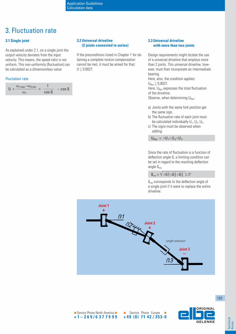
3. Fluctuation rate3.1 Single joint

As explained under 2.1, on a single joint the output velocity deviates from the input velocity. This means, the speed ratio is not uniform. This non-uniformity (fl uctuation) can be calculated as a dimensionless value:

Fluctation rate

U

=

2 max – 2 min =

1 – cos ß 1 cos ß

3.2 Universal driveline (2 joints connected in series)

If the preconditions listed in Chapter 1 for ob-taining a complete motion compensationcannot be met, it must be aimed for that:U 0,0027.

Joint 1+

Joint 2+

Joint 3–

Since the rate of fl uctuation is a function ofdefl ection angle ß, a limiting condition canbe set in regard to the resulting defl ectionangle ßres

ßres = ß 21 ß 2

2 ß 23 3°

ßres corresponds to the defl ection angle ofa single joint if it were to replace the entiredriveline.

3.3 Universal driveline with more than two joints

Design requirements might dictate the use of a universal driveline that employs more than 2 joints. This universal driveline, how-ever, must then incorporate an intermediate bearing.Here, also, the condition applies:URes 0,0027.Here, URes expresses the total fl uctuationof the driveline.Observe, when determining URes:

a) Joints with the same fork position get the same sign.b) The fl uctuation rate of each joint must be calculated individually U1, U2, U3.c) The signs must be observed when adding:

URes = U 1U 2 U 3

Length extension

170

Tech

nica

lAn

nex


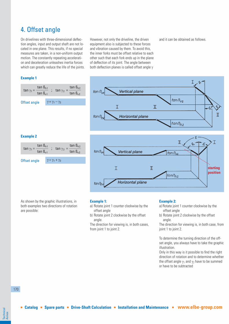
On drivelines with three-dimensional defl ec-tion angles, input and output shaft are not lo-cated in one plane. This results, if no special measures are taken, in a non-uniform output motion. The constantly repeating accelerati-on and deceleration unleashes inertia forces which can greatly reduce the life of the joints.

However, not only the driveline, the driven equipment also is subjected to these forces and vibration caused by them. To avoid this, the inner forks must be offset relative to eachother such that each fork ends up in the plane of defl ection of its joint. The angle between both defl ection planes is called offset angle

and it can be obtained as follows.

4. Offset angle

Example 1

tan 1

=

tan ßh1 ; tan 2

=

tan ßh2

tan ßv1 tan ßv2

Offset angle = 1 – 2

Example 2

tan 1

=

tan ßh1 ; tan 2

=

tan ßh2

tan ßv1 tan ßv2

Offset angle = 1 + 2

As shown by the graphic illustrations, inboth examples two directions of rotationare possible:

Example 1:a) Rotate joint 1 counter clockwise by the offset angleb) Rotate joint 2 clockwise by the offset angle.The direction for viewing is, in both cases, from joint 1 to joint 2.

Example 2:a) Rotate joint 1 counter clockwise by the offset angleb) Rotate joint 2 clockwise by the offset angle.The direction for viewing is, in both case, from joint 1 to joint 2.

To determine the turning direction of the off-set angle, you always have to take the graphic illustration.Only in this way is it possible to fi nd the right direction of rotation and to determine whether the offset angle 1 and 2 have to be summed or have to be subtracted

Vertical plane

Horizontal plane

Vertical plane

Horizontal plane

starting position

171


Tech

nica

lAn

nex



5.3 Caused by axial displacement forces

If a driveline with an adjustable spline is being changed in length while under torque, in both cases, Z- or W confi guration, addition bearing loads are introduced, resulting from the friction caused in the spline. The axial dis-

placement force Pa responsible for these bearing loads is calculated as follows:

dm is the spline pitch diameter, Ü the spline

overlap. Depending on confi guration and lubri-cation, the coeffi cient of friction for steel onsteel must be assumed to range from 0.11 to 0.15. Plastic coated splines have considerably better sliding characteristics. Here, the fric-tion value is approximately 0.08. Rilsan coated splines are available from size 0.109 up.

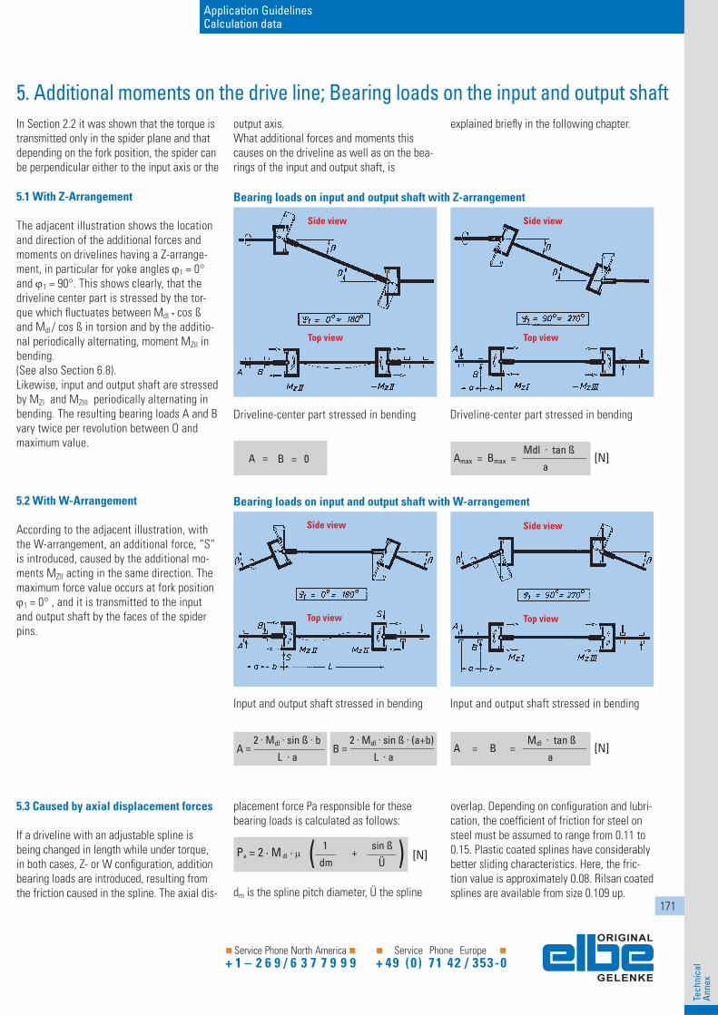
In Section 2.2 it was shown that the torque is transmitted only in the spider plane and that depending on the fork position, the spider can be perpendicular either to the input axis or the

output axis.What additional forces and moments this causes on the driveline as well as on the bea-rings of the input and output shaft, is

explained briefl y in the following chapter.

5. Additional moments on the drive line; Bearing loads on the input and output shaft

5.1 With Z-Arrangement

The adjacent illustration shows the location and direction of the additional forces and moments on drivelines having a Z-arrange-ment, in particular for yoke angles 1 = 0° and 1 = 90°. This shows clearly, that the driveline center part is stressed by the tor-que which fl uctuates between MdI · cos ß and MdI/ cos ß in torsion and by the additio-nal periodically alternating, moment MZII in bending. (See also Section 6.8).Likewise, input and output shaft are stressed by MZI and MZIII periodically alternating in bending. The resulting bearing loads A and B vary twice per revolution between O and maximum value.

5.2 With W-Arrangement

According to the adjacent illustration, with the W-arrangement, an additional force, “S“ is introduced, caused by the additional mo-ments MZII acting in the same direction. The maximum force value occurs at fork position1 = 0° , and it is transmitted to the input and output shaft by the faces of the spider pins.

Side view

Top view

Side view

Top view

Side view

Top view

Side view

Top view

Driveline-center part stressed in bending

A =

2 . Mdl . sin ß . b

L . aB

=

2 . Mdl . sin ß . (a+b)

L . a

Driveline-center part stressed in bending

A = B = Mdl . tan ß

a[N]

Amax = Bmax = Mdl . tan ß

a[N]

Input and output shaft stressed in bending Input and output shaft stressed in bending

A = B = 0

Bearing loads on input and output shaft with Z-arrangement

Bearing loads on input and output shaft with W-arrangement

Pa = 2 · M dI · 1

+ sin ß

dm Ü[N]( )

172

Tech

nica

lAn

nex


To size universal drivelines properly, various conditions and factors must be considered. In view of the multitude of possible applications, exact, generally valid rules cannot be

provided. The following information is there-fore used for the fi rst rough determination of size. In case of doubt, we will gladly compu-te the required joint sizes for you and, in this

context, we like to refer to the technical ques-tionnaires starting on page 189.

6. Fundamental data for sizing of universal drivelines

6.1 Torques

The max. permitted torques Mdmax stated for the individual drive-shaft sizes apply normally only for short-term peak loads.Mdnom: Nominal torque for pre-selection on the basis of the operating moment. Mdlim: Limit torque that may be transmitted temporarily from the universal-drive-joint at limited frequency without functional damage.

The respective permissible torque has to be cal-culated individually depending on the remaining operating data, such as shock loads, angle of de-fl ection, rotation,etc. (See item 6.2 and 6.3)

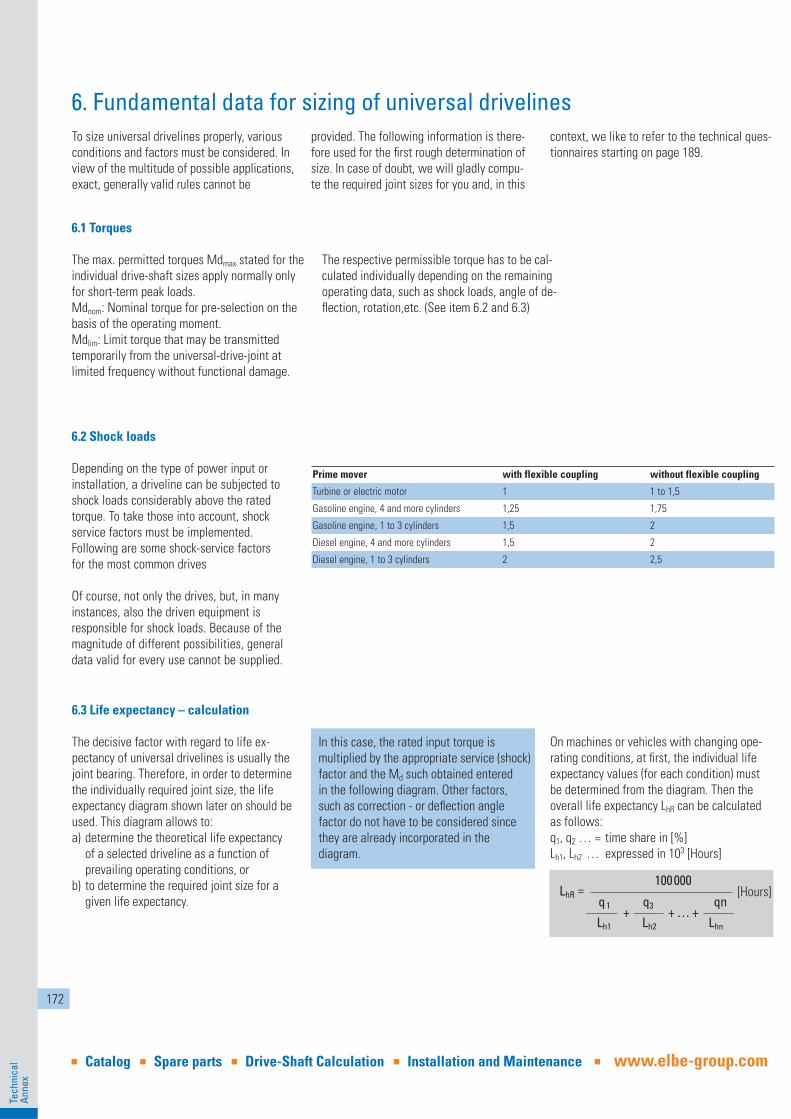
6.2 Shock loads

Depending on the type of power input or installation, a driveline can be subjected to shock loads considerably above the rated torque. To take those into account, shockservice factors must be implemented. Following are some shock-service factors for the most common drives

Of course, not only the drives, but, in many instances, also the driven equipment is responsible for shock loads. Because of the magnitude of different possibilities, general data valid for every use cannot be supplied.

6.3 Life expectancy – calculation

The decisive factor with regard to life ex-pectancy of universal drivelines is usually the joint bearing. Therefore, in order to determine the individually required joint size, the life expectancy diagram shown later on should be used. This diagram allows to:a) determine the theoretical life expectancy of a selected driveline as a function of prevailing operating conditions, orb) to determine the required joint size for a given life expectancy.

Prime mover with flexible coupling without flexible coupling

Turbine or electric motor 1 1 to 1,5

Gasoline engine, 4 and more cylinders 1,25 1,75

Gasoline engine, 1 to 3 cylinders 1,5 2

Diesel engine, 4 and more cylinders 1,5 2

Diesel engine, 1 to 3 cylinders 2 2,5

In this case, the rated input torque is multiplied by the appropriate service (shock) factor and the Md such obtained entered in the following diagram. Other factors, such as correction - or defl ection angle factor do not have to be considered since they are already incorporated in the diagram.

On machines or vehicles with changing ope-rating conditions, at fi rst, the individual life expectancy values (for each condition) must be determined from the diagram. Then the overall life expectancy LhR can be calculated as follows:q1, q2 … = time share in [%]Lh1, Lh2 … expressed in 103 [Hours]

LhR

=

100000

q 1 +

q3 + . . . +

qn

Lh1 Lh2 Lhn

[Hours]

173


Tech

nica

lAn

nex



6.4 Life expectancy-Diagram

In view of the multitude of applications, it is not possible to determine the suitability of a driveline by tests. Therefore, the selection andanalysis of the required joint size is done by calculations. These are based on the compu-tation of the dynamic load carrying capacity of full rotation needle - and roller bearings ac-cording to ISO recommendation R 281. The life expectancy diagrams shown in the catalogue are based on this recommendation and also on an equation formula especially suited for obtaining nominal life expectancy on universal joints. The thus obtained life expectancy lists the hours of operation that will be reached or exceeded by 90% of a larger number of equi-valent universal joint bearings.

There are also methods of obtaining the mo-difi ed life expectancy. In this case varying sur-vival probabilities, material quality and ope-rating conditions are taken into account. The present technical know how does not allow statements to be made about variations in life expectancy performance resulting from differ-ences in steel quality (grain, hardness, impu-rities). For this reason, no guidelines have been set in the International Standards.

All pertinent operating conditions, such as operating temperature, lubrication intervals, the type of grease used and its viscosity in operation, must also be considered. Since these factors vary from case to case, it is not possible to determine the modifi ed life

expectancy and accordingly, a life expectancy diagram valid for universal use.

The two following life expectancy diagramswill allow you to roughly determine the nomi-nal life expectancy.

If the defl ection angle is smaller than ß = 3°, ß = 3 should be used. Otherwise, the obtained result will be less accurate.

If it is necessary to determine the life expec-tancy accurately, kindly consult the ELBE Engineering Department.

174

Tech

nica

lAn

nex


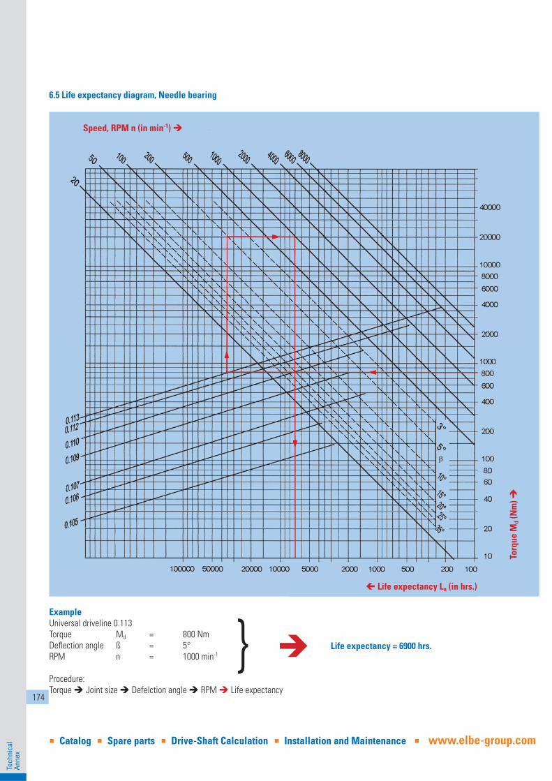
6.5 Life expectancy diagram, Needle bearing

Speed, RPM n (in min-1)

Torq

ue M

d (N

m)

Life expectancy Ln (in hrs.)

ExampleUniversal driveline 0.113Torque Md = 800 NmDefl ection angle ß = 5°RPM n = 1000 min-1

Procedure:Torque Joint size Defelction angle RPM Life expectancy

} Life expectancy = 6900 hrs.

175


Tech

nica

lAn

nex



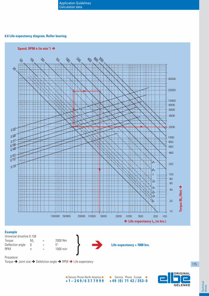
6.6 Life expectancy diagram, Roller bearing

ExampleUniversal driveline 0.158Torque Md = 2000 NmDefl ection angle ß = 5°RPM n = 1000 min-

Procedure:Torque Joint size Defelction angle RPM Life expectancy

} Life expectancy = 7000 hrs.

Speed, RPM n (in min-1)

Torq

ue M

d (N

m)

Life expectancy Ln (in hrs.)

176

Tech

nica

lAn

nex


6.8 Critical speeds

As shown in 5.1, the center part of the an-gled driveline, when transmitting torque, is stressed periodically in bending by additional moment MZII. This incites the center part to vibrate. If the frequency of this bending vibra-tion approaches the natural frequency of the driveline, maximum stress in all components, buckling of the shaft and development of noi-se will result.

To avoid this, long and fast running drivelines must be checked for critical bending vibration speeds. The critical, fi rst order bending vibra-tion speed of a driveline employing tubing can be roughly calculated as follows:

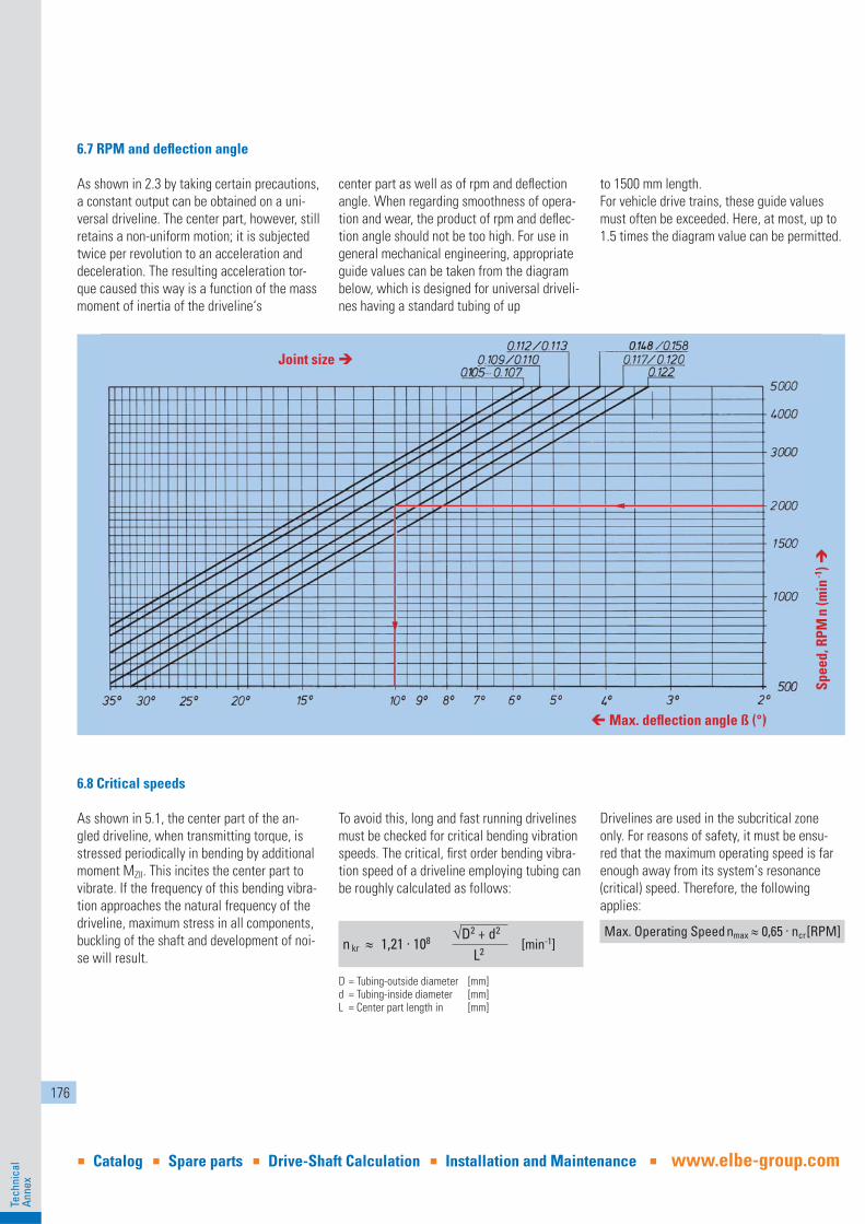
6.7 RPM and defl ection angle

As shown in 2.3 by taking certain precautions, a constant output can be obtained on a uni-versal driveline. The center part, however, still retains a non-uniform motion; it is subjected twice per revolution to an acceleration and deceleration. The resulting acceleration tor-que caused this way is a function of the mass moment of inertia of the driveline‘s

center part as well as of rpm and defl ection angle. When regarding smoothness of opera-tion and wear, the product of rpm and defl ec-tion angle should not be too high. For use in general mechanical engineering, appropriate guide values can be taken from the diagram below, which is designed for universal driveli-nes having a standard tubing of up

to 1500 mm length.For vehicle drive trains, these guide values must often be exceeded. Here, at most, up to 1.5 times the diagram value can be permitted.

Spee

d, R

PM n

(min

-1)

Joint size

Max. defl ection angle ß (°)

n kr 1,21 . 108

D2 + d2

[min-1] L2

D = Tubing-outside diameter [mm]d = Tubing-inside diameter [mm]L = Center part length in [mm]

Drivelines are used in the subcritical zone only. For reasons of safety, it must be ensu-red that the maximum operating speed is far enough away from its system‘s resonance (critical) speed. Therefore, the following applies:

Max. Operating Speed nmax 0,65 . ncr[RPM]

177


Tech

nica

lAn

nex



6.9 Larger tubing diameters

The critical bending vibration speed of a dri-veline is, as can be seen from the critical rpm formula, a function of tubing diameters and length of center part. By going to larger tubing diameters, the critical speed of a driveline can be increased. However, the diameter increase must remain within defi ned limits since a cer-tain relationship between tubing dimensions and joint size must be adhered to.

The dimension sheets of the different driveli-ne models list the possible tubing dimensions for each size. In all the cases where a single driveline is insuffi cient, multiple arrangements with intermediate bearings must be used.

It must be noted that larger tubing diameters are feasible only above a certain shaft length. The following minimum lengths can be used as an angle line.

Flange diameter [mm] Up to 65 75 to 100 120 to 180Min. length S [mm] 650 950 1250

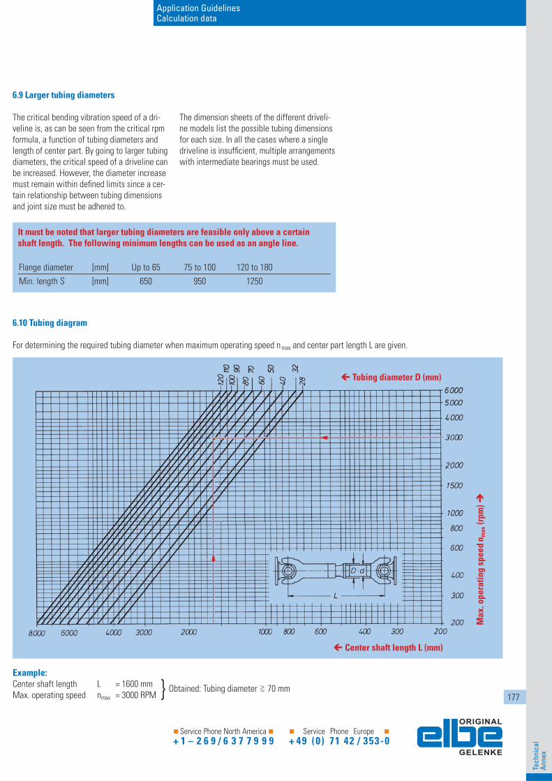
6.10 Tubing diagram

For determining the required tubing diameter when maximum operating speed n max and center part length L are given.

Max

. ope

ratin

g sp

eed

n max

(rpm

)

Tubing diameter D (mm)

Center shaft length L (mm)

Example:Center shaft length L = 1600 mmMax. operating speed nmax = 3000 RPM

Obtained: Tubing diameter 70 mm}

178

Tech

nica

lAn

nex


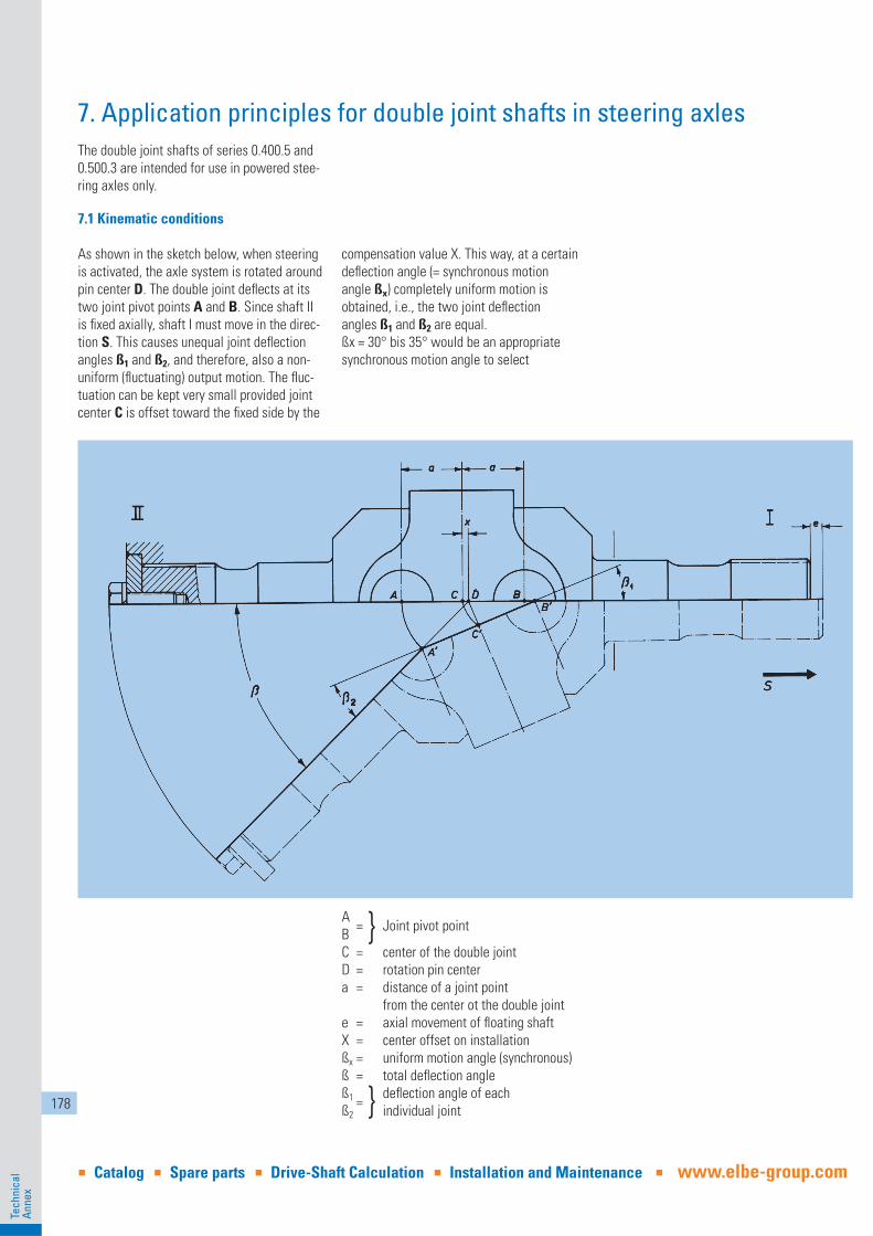
7. Application principles for double joint shafts in steering axlesThe double joint shafts of series 0.400.5 and 0.500.3 are intended for use in powered stee-ring axles only.

7.1 Kinematic conditions

As shown in the sketch below, when steering is activated, the axle system is rotated around pin center D. The double joint defl ects at its two joint pivot points A and B. Since shaft II is fi xed axially, shaft I must move in the direc-tion S. This causes unequal joint defl ection angles ß1 and ß2, and therefore, also a non-uniform (fl uctuating) output motion. The fl uc-tuation can be kept very small provided joint center C is offset toward the fi xed side by the

compensation value X. This way, at a certain defl ection angle (= synchronous motion angle ßx) completely uniform motion is obtained, i.e., the two joint defl ection angles ß1 and ß2 are equal.ßx = 30° bis 35° would be an appropriate synchronous motion angle to select

A = Joint pivot pointBC = center of the double jointD = rotation pin centera = distance of a joint point from the center ot the double jointe = axial movement of fl oating shaftX = center offset on installationßx = uniform motion angle (synchronous)ß = total defl ection angleß1 = defl ection angle of eachß2 individual joint

}

}

179


Tech

nica

lAn

nex



7.2 Center offset value x and max. slide movement e

The center offset X required for smooth outputcan be derived from distance a and synchro-nous motion angle ß:

Series 0.500, synchronous motion angle ßx = 32°

Calculated center offset value X for individual joint sizes:Series 0.400, synchronous motion angle ßx = 35°

7.3 Sizing of double joint shafts

Max. possible torque should be used for de-termining the required joint size. This could be the input torque, calculated from prime mo-ver output, gear ratio and power distribution, or also the tire slippage torque, derived from allowable axle loading, static tire radius and coeffi cient of friction. The lower of the two va-lues represents the maximum operating tor-que which should be used for determining the

proper joint size. The double joint shaft select-ed this way will have adequate life expectan-cy, since the time percentage of maximum loa-ding is usually low.

7.4 Loads on the shaft bearing

Double joint shafts, when not centered, must have a bearing support at both shaft halves right next to the joint with one shaft half fi xed axially and the other fl oating axially. When torque is being transmitted, additional forces occur which must be taken into account when sizing the bearings.

Joint size 0.408 0.409 0.411 0.412

Deflection angle ß° 50 50 50 50

x [mm] 1,5 1,7 2,0 2,2

Joint size 0.509 0.510 0.511 0.512 0.513 0.515 0.516 0.518

Deflection angle ß° 42 | 47 | 50 42 | 47 42 | 47 42 | 47 42 | 47 42 | 47 42 | 47

x [mm] 1,3 | 1,3 | 1,6 1,5 | 1,6 1,6 | 1,7 1,7 | 1,8 1,9 | 2,0 2,1 | 2,2 2,2 | 2,3

Sliding motion e at defl ection angle ß, and also as a function of distance a and uniform motion angle ßx, can be calculated as follows:

Series 0.500, uniform synchronous motion angle ßx = 32°

Max. slide motion e for the individual joint sizes:Series 0.400, synchronous motion angle ßx = 35°

Joint size 0.408 0.409 0.411 0.412

Deflection angle ß° 50 50 50 50

e [mm] 6,5 7,2 8,3 9,2

Joint size 0.509 0.510 0.511 0.512 0.513 0.515 0.516 0.518

Deflection angle ß° 42 | 47 | 50 42 | 47 42 | 47 42 | 47 42 | 47 42 | 47 42 | 47

e [mm] 4,5 | 6,0 | 7,9 5,2 | 6,9 5,8 | 7,8 6,1 | 8,1 6,7 | 9,0 7,3 | 9,7 7,8 | 10,5

X = – aa

cos ßx

2

( )ßx2e = 2 a

ß2

ß2

ß2

ßx2

cos– 1

sin2 + cos2 – sin2 · cos2

180

Tech

nica

lAn

nex


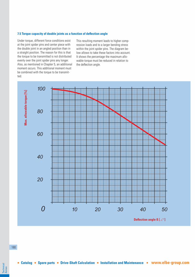
Under torque, different force conditions exist at the joint spider pins and center piece with the double joint in an angled position than in a straight position. The reason for this is that the torque to be transmitted is not distributed evenly over the joint spider pins any longer. Also, as mentioned in Chapter 5, an additional moment occurs. This additional moment must be combined with the torque to be transmit-ted.

This resulting moment leads to higher comp-ression loads and to a larger bending stress within the joint spider pins. The diagram be-low allows to take these factors into account. It shows the percentage the maximum allo-wable torque must be reduced in relation to the defl ection angle.

7.5 Torque capacity of double joints as a function of defl ection angle

Max

. allo

wab

le to

rque

[%]

Defl ection angle ß [ ]

181


Tech

nica

lAn

nex



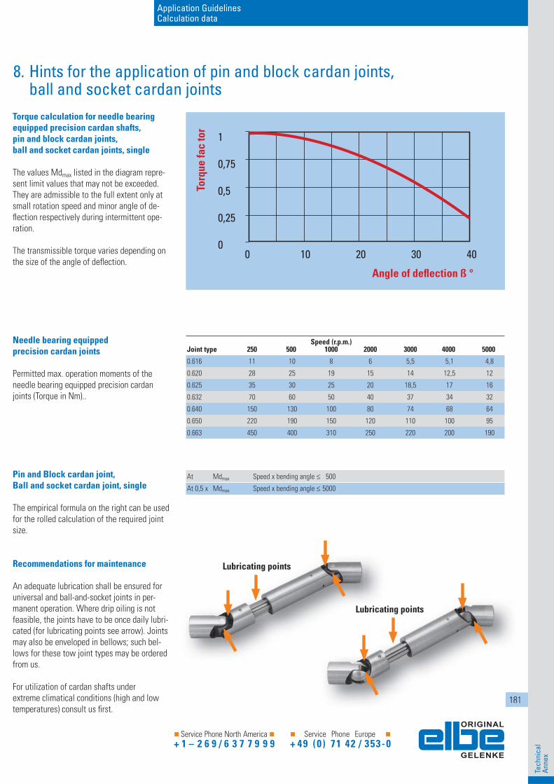
8. Hints for the application of pin and block cardan joints, ball and socket cardan jointsTorque calculation for needle bearing equipped precision cardan shafts, pin and block cardan joints, ball and socket cardan joints, single

The values Mdmax listed in the diagram repre-sent limit values that may not be exceeded. They are admissible to the full extent only at small rotation speed and minor angle of de-fl ection respectively during intermittent ope-ration.

The transmissible torque varies depending on the size of the angle of defl ection.

Needle bearing equipped precision cardan joints

Permitted max. operation moments of the needle bearing equipped precision cardan joints (Torque in Nm)..

Pin and Block cardan joint,Ball and socket cardan joint, single

The empirical formula on the right can be used for the rolled calculation of the required joint size.

Recommendations for maintenance

An adequate lubrication shall be ensured for universal and ball-and-socket joints in per-manent operation. Where drip oiling is not feasible, the joints have to be once daily lubri-cated (for lubricating points see arrow). Joints may also be enveloped in bellows; such bel-lows for these tow joint types may be ordered from us.

For utilization of cardan shafts under extreme climatical conditions (high and low temperatures) consult us fi rst.

Speed (r.p.m.)Joint type 250 500 1000 2000 3000 4000 5000

0.616 11 10 8 6 5,5 5,1 4,8

0.620 28 25 19 15 14 12,5 12

0.625 35 30 25 20 18,5 17 16

0.632 70 60 50 40 37 34 32

0.640 150 130 100 80 74 68 64

0.650 220 190 150 120 110 100 95

0.663 450 400 310 250 220 200 190

Torq

ue fa

c to

r

Angle of defl ection ß °

1

0,75

0,5

0,25

00 10 20 30 40

At Mdmax Speed x bending angle 500

At 0,5 x Mdmax Speed x bending angle 5000

Lubricating points

18

Lubricating points

Documents

2. Motion relationships and torques