Embed Size (px)
Citation preview

1
Acoustic and biological trends on coral reefs off Maui, Hawaii 1
Maxwell B. Kaplan1*, Marc O. Lammers2,3, Eden Zang2, T. Aran Mooney1 2
3
1Biology Department, Woods Hole Oceanographic Institution, Woods Hole, MA, 02543, USA 4
5
2Oceanwide Science Institute, Honolulu, HI, 96839 USA 6
7
3Hawaii Institute of Marine Biology, Kaneohe, HI, 96744, USA 8
9
*Corresponding author: [email protected] 10
11
Key words: Coral reefs, Soundscapes, Biodiversity, Soniferous 12

2
Abstract 13
Coral reefs are characterized by high biodiversity and evidence suggests that reef soundscapes 14
reflect local species assemblages. To investigate how sounds produced on a given reef relate to 15
abiotic and biotic parameters and how that relationship may change over time, an observational 16
study was conducted between September 2014 and January 2016 at seven Hawaiian reefs that 17
varied in coral cover, rugosity, and fish assemblages. The reefs were equipped with temperature 18
loggers and acoustic recording devices that recorded on a 10% duty cycle. Benthic and fish 19
visual survey data were collected four times over the course of the study. On average, reefs 20
ranged from 0 to 80% live coral cover, although changes between surveys were noted, in 21
particular during the major El Niño-related bleaching event of October 2015. Acoustic analyses 22
focused on two frequency bands (50–1200 Hz and 1.8–20.5 kHz) that corresponded to the 23
dominant spectral features of the major sound-producing taxa on these reefs, fish and snapping 24
shrimp, respectively. In the low-frequency band, the presence of humpback whales (December–25
May) was a major contributor to sound level, whereas in the high-frequency band sound level 26
closely tracked water temperature. On shorter timescales, the magnitude of the diel trend in 27
sound production was greater than that of the lunar trend, but both varied in strength among 28
reefs, which may reflect differences in the species assemblages present. Results indicated that the 29
magnitude of the diel trend was related to fish densities at low frequencies and coral cover at 30
high frequencies; however, the strength of these relationships varied by season. Thus, long-term 31
acoustic recordings capture the substantial acoustic variability present in coral-reef ecosystems 32
and provide insight into the presence and relative abundance of sound-producing organisms. 33
34
Introduction 35

3
Coral reefs vary in their species assemblages in space and time (Parravicini et al. 2013; 36
Williams et al. 2015) and identifying the drivers of this variability has long been a focus of the 37
ecological literature. Much effort has gone into characterizing links between biophysical 38
attributes of coral reefs and fish species assemblages. Parameters such as depth, substrate 39
complexity (rugosity), live coral cover, and coral species richness appear to be important 40
correlates with fish species richness and abundance (McCormick 1994; Friedlander et al. 2003; 41
Messmer et al. 2011; Komyakova et al. 2013). 42
Just as the biological composition of coral reefs changes over time, so too do the 43
associated ambient soundscapes (Staaterman et al. 2014; Kaplan et al. 2015; Nedelec et al. 44
2015). For example, in an approximately year-long study of two Caribbean reefs, sound levels 45
were found to vary on diel and lunar scales (Staaterman et al. 2014). However, the relationship to 46
species present was not well characterized, which limited understanding of the influence of 47
species assemblages on local soundscapes. Contemporaneous work sought to link visual survey 48
data to soundscape measurements and found a relationship between the strength of diel trends in 49
sound production to fish density and coral cover on Caribbean reefs (Kaplan et al. 2015). 50
However, that study was relatively short (four months) and was conducted using only three reefs 51
(Kaplan et al. 2015). While others have compared acoustic parameters to biophysical variables 52
such as coral cover, fish density, and sea state across several reefs (Nedelec et al. 2014; Bertucci 53
et al. 2016), this has often come with the trade-off of using relatively brief recordings that likely 54
overlook the appreciable variation in sound cues over longer timescales (Radford et al. 2008; 55
Staaterman et al. 2014; Kaplan et al. 2015). 56
Collectively, these studies present initial characterizations of some of the putative drivers 57
of this acoustic variability, such as water temperature and the biota present, suggesting a link 58

4
between reef species assemblages and the local soundscape. Individually, however, these studies 59
often do not adequately characterize the temporal or spatial variability that is likely present. For 60
example, the relevant factors influencing biological sound production may vary in importance 61
over multiple timescales and among communities of sound-producing organisms (Radford et al. 62
2008; Radford et al. 2014). Thus, data collected from several sites over relatively long timescales 63
are most likely to yield insight into the relationships between biodiversity and ambient 64
soundscapes. 65
Despite the limitations of the aforementioned studies, this growing body of work suggests 66
that monitoring the sounds produced by the diverse array of soniferous coral-reef organisms may 67
be a cost-effective and efficient means of assessing reef community assemblages and their 68
changes over time (Lammers et al. 2008; Radford et al. 2014). Acoustic observations could 69
supplement or reduce the need for frequent, traditional, diver-based visual surveys. However, to 70
develop the capability to infer species assemblages and ecological dynamics from acoustic data 71
(i.e., inverse prediction), it is first necessary to examine the relationship between biological 72
sounds on reefs and fundamental ecological parameters, such as fish species richness and 73
abundance and benthic cover. 74
In recent years, there has been interest in applying acoustic biodiversity metrics 75
developed for terrestrial ecosystems to marine soundscapes (e.g., Parks et al. 2014; Bertucci et 76
al. 2016; Staaterman et al. 2017); however, there has been little compelling evidence to suggest 77
that such metrics provide valuable information not available from more traditional measurements 78
like sound pressure level (Staaterman et al. 2017). For example, a recent effort attempted to 79
apply the acoustic complexity index (ACI) to recordings of coral reefs (Bertucci et al. 2016), but 80
its utility was not obvious. Higher ACI values were found in recordings of marine protected 81

5
areas (MPAs) compared to non-MPAs. However, there were no significant differences between 82
protected and unprotected areas in any visual survey parameter, suggesting that differences in 83
ACI values between protected and non-protected reefs were not reflective of the species 84
assemblages observed in the study (Bertucci et al. 2016). Furthermore, previous work has shown 85
that these indices may be predominately influenced by snapping shrimp activity, which is a 86
major component of coral-reef and temperate soundscapes (Kaplan et al. 2015). At present, more 87
traditional bioacoustic metrics such as sound pressure level (SPL) and the variability in sound 88
level in specific frequency bands over time are likely to be more robust and easier to comprehend 89
than indices such as the ACI. 90
In addition to biological sounds, anthropogenic noise can modify reef soundscapes in 91
significant ways (e.g., Kaplan and Mooney 2015). The extent of human activity can and does 92
vary among reefs because of differing degrees of remoteness, protection (e.g., areas closed to 93
vessels), and heterogeneous utilization rates. Recent work suggests that noise from small vessels 94
may increase the predation risk for some reef fish (Simpson et al. 2016). Accordingly, these 95
human-mediated elements could also influence biological sound production and species 96
assemblages on coral reefs. 97
To parameterize the factors that might influence sound production on reefs across space, 98
time and ecological gradients such as live coral cover and fish density, long-term assessment of a 99
range of geographically and ecologically disparate reefs is needed. This study measured 100
soundscapes and examined visually observable species assemblages at seven Hawaiian reefs that 101
varied in benthic cover and fish species assemblages over an approximately 16-month period. 102
Here, we present results from visual and acoustic surveys of these reefs and describe a new 103
method to quantitatively assess the magnitude of sound production on coral reefs. 104

6
105
Methods 106
Site selection 107
Reefs were selected for study on the west side of Maui, Hawaii, in September 2014. The sites 108
were chosen to be similar in depth but different in terms of benthic cover, fish species richness 109
and abundance, structural complexity, geographic location, and degree of protection. These 110
parameters were assessed in an ad hoc manner during the site selection period and confirmed ex 111
post using visual surveys described below. Because of an instrument malfunction, one reef was 112
ultimately excluded from the study, leaving six reefs and one sandy control site (MM17) for data 113
analysis (Fig. 1a; Table 1). Of these, one (Ahihi) was completely closed to vessel traffic, two 114
were Marine Life Conservation Districts closed to some forms of fishing (Honolua and 115
Molokini), and one was a Fishery Management Area closed to the fishing of herbivores 116
(Kahekili). 117
Visual surveys 118
Visual surveys were carried out at each study reef in September 2014, February/March 2015, 119
October 2015, and January 2016. Data were collected by the same two divers for the duration of 120
the study to ensure consistency among surveys, with each specializing in either fish or benthic 121
surveys. Fish sizing estimates were calibrated underwater using artificial fish models and inter-122
observer comparisons prior to data collection. Survey methods were modified from Kaplan et al. 123
(2015). Four benthic transects per reef were conducted using a 10-m sinking lead line that 124
followed the contours of the reef. Each transect started adjacent to the acoustic recorder moored 125
at that reef and fanned out in a radial pattern. At each 10-cm increment, benthic cover was 126
recorded as one of the following categories: live coral (identified to genus), macroalgae, turf 127

7
algae, sand, bare rock, dead coral, bleached coral, and other invertebrates. All benthic transects 128
were compiled for each survey using the following categories: live coral, bleached coral, 129
macroalgae, crustose coralline algae, turf algae, and “other” (e.g., bare rock, sand, dead coral, 130
other invertebrates). 131
To quantify structural complexity the straight-line distance of the lead line was measured 132
with a fiberglass tape, and rugosity was then calculated as the ratio of the length of the lead line 133
to the length of the straight-line distance. 134
Belt transect surveys for fish were carried out concurrently. These consisted of four 135
transects (30 m long by 2.5 m on either side of the transect). Start points adjacent to the acoustic 136
recorder were selected randomly. Each fish transect took approximately 10 min to complete. The 137
surveyor first swam rapidly along the transect line, recording larger mobile fishes transiting the 138
line, mid-water species, and any conspicuous, rare, or uncommon species. They then turned 139
around and returned along the transect line, slowly and carefully recording all other fishes with a 140
focus on cryptic species. Each observed fish was identified to species and categorized by size 141
(total length) in the following bins: A (0–10 cm), B (11–15 cm), C (16–20 cm), D (21–30 cm), E 142
(31–40 cm), and F (>40 cm). Fish survey data were combined across transects and summarized 143
by species and size classes. Species that have previously been identified as soniferous (Tricas 144
and Boyle 2014) were noted as such in the data set. 145
Acoustic data 146
Acoustic data were collected at each reef using ecological acoustic recorders (EARs; Lammers et 147
al. 2008) equipped with an SQ26-01 hydrophone (Sensor Technology Ltd., Collingwood, ON, 148
Canada) with a sensitivity of approximately -193.5 dBV re 1 µPa and configured with 47.5 dB of 149
gain. Recordings were collected at a sample rate of 50 kHz (25 kHz at Molokini) on a 10% duty 150

8
cycle (30 s/300 s). For all deployments, EARs were affixed to concrete blocks using hose clamps 151
and cable ties and placed in sand patches adjacent to or within a reef (Fig. 1b). Hydrophones 152
were approximately 6 inches above the bottom. All EARs, except at Molokini, were deployed in 153
September 2014, refurbished in February/March 2015 and July 2015, and recovered in January 154
2016. The Molokini EAR was involved in a separate study and was deployed and refurbished on 155
a different schedule (November 2013, June 2014, October 2014, February 2015, October 2015, 156
October 2016). 157
Analyses were carried out in MATLAB 9.1 (MathWorks, Natick, MA). Sound files were 158
corrected for hydrophone sensitivity and resampled to 44 kHz for improved computational 159
efficiency and to retain frequencies of interest (except for recordings from Molokini, which were 160
not resampled because of the lower sample rate). An initial review of the recordings indicated 161
that in some cases clipping was present as a result of high-amplitude shrimp snaps. Accordingly, 162
every 30 s sound file was split into 100 ms windows and every window that contained 163
normalized voltage readings of ±0.99, indicative of the presence of clipping, was automatically 164
excluded (Table 2). The entire file was discarded in cases where fewer than 150 windows (i.e., 165
15 s) were retained. All remaining windows of each retained sound file were individually 166
analyzed as follows. Root-mean-square SPL (dB re 1 µPa) was calculated in two frequency 167
bands—low (50–1200 Hz) and high (1800–20500 Hz; 2000–12000 Hz for Molokini)—using 168
four-pole Butterworth bandpass filters. These frequency bands were chosen to correspond with 169
the published frequency ranges of fish calls and snapping shrimp pulses, respectively (Au and 170
Banks 1998; Tricas and Boyle 2014). The intermediate frequencies (1200–1800 Hz) were not 171
assessed given the paucity of biological signals of interest in this range and to provide a spectral 172
buffer between the frequency bands analyzed. To obtain an average SPL value for each sound 173

9
file, the mean SPL of the first 150 windows was then computed (on the linear scale in Pascals). 174
While a narrower bandwidth at high frequencies was used for Molokini, this choice did not affect 175
results because no explicit comparisons of sound levels were made among reefs. 176
To ensure that these analyses focused on sounds of biological origin, vessel and other 177
extrinsic anthropogenic noise was identified and excised. This was done individually for each 178
reef by visually identifying and aurally confirming such sounds in long-term spectral average 179
plots produced in Triton version 1.91 (Scripps Whale Acoustics Lab, San Diego, CA). 180
Humpback whales (Megaptera novaengliae), present during the winter months 181
(approximately December–May), represented an undesired biological sound source, in particular 182
when making among-reef comparisons of low-frequency sound, where humpback whale song 183
overlaps with and can mask lower amplitude fish calls. Thus, low-frequency sound data were not 184
considered between 1 December and 30 April except in visualizations of daily average levels. 185
Comparisons between diel and lunar periodicity were made by constructing periodograms 186
of the SPL time series in both frequency bands. Linear interpolation to fill in missing data was 187
necessary to ensure a constant sampling rate of one recording per 5 min or 288 samples d–1. This 188
was done for all reefs; results from Kahekili, generally representative of all reefs, are presented 189
here. 190
Crepuscular periodicity was a distinct feature of these acoustic data. To quantify the 191
magnitude of those diel changes in sound level, the median sound level at each sampling time 192
(i.e., 288 times d–1) was computed by month for the low- and high-frequency bands. This yielded 193
monthly median curves of sound level by time of day in each frequency band. These curves were 194
normalized to a zero minimum sound level to facilitate comparisons among reefs irrespective of 195
background noise levels. Subsequently, the total area under the curve at dawn and dusk was 196

10
computed in MATLAB using the trapz function to quantify the strength of the diel trend. Dawn 197
was defined as 1 h before to 15 min after sunrise and dusk was defined as 15 min before to 1 h 198
after sunset. All other times were not considered. The timing of sunrise and sunset at each reef 199
was identified for each day of the deployment in MATLAB using the reef coordinates and the 200
suncycle tool. 201
Environmental parameters 202
Temperature data loggers (HOBO pendant models UA-001-64 and UA-002-64, Onset Computer 203
Corporation, Bourne, MA), sampling every 10 min, were deployed alongside EARs at all reefs 204
for the duration of the study, except for Molokini, where temperature data were only collected 205
from July 2015 until January 2016. Wind speeds were gathered from a nearby NOAA National 206
Ocean Service weather buoy (20.895°N, 156.469°W). Lunar illumination data were obtained 207
from the US Naval Observatory website (http://aa.usno.navy.mil/data/docs/MoonFraction.php). 208
Statistical analysis 209
To investigate whether there were differences in fish assemblage characteristics within and 210
among reefs, Bray–Curtis dissimilarity values were computed and visualized using non-metric 211
multidimensional scaling (MDS) routines implemented in MATLAB. Correlations between wind 212
speed and SPL were assessed using hourly averages for each variable. Correlations between 213
temperature and SPL were assessed using daily averages for each variable. 214
Only acoustic data collected within 30 d of the visual survey dates were used in 215
comparisons with visual surveys to limit potential impact of temporal changes in the biological 216
community of the reef over longer timescales. Accordingly, high-frequency correlations were 217
made at each of the four visual survey periods whereas low-frequency correlations were only 218
made for visual surveys conducted in September 2014 and October 2015, to avoid including any 219

11
acoustic data that contained humpback whale song (Au et al. 2000). All correlations were tested 220
for significance using linear regression models. 221
222
Results 223
Benthic cover varied among and within the study reefs (Fig. 2a). Live coral cover was 224
generally highest at Molokini and Olowalu and lowest (i.e., zero) at MM17, a sandy non-reef 225
control site. Honolua had the highest proportion of turf algae and Ahihi had the highest crustose 226
coralline algal cover. Within-reef cover was relatively consistent over time except during the 227
October 2015 survey, when an appreciable proportion of live coral was bleached at every reef, 228
except sand-dominated MM17. Reefs with highest live coral cover, such as Molokini and 229
Olowalu, also had the greatest proportion of bleaching. By January 2016, most of the bleaching 230
had diminished and recovery was observable at every bleached reef, although some, such as Red 231
Hill, suffered mortality. 232
Corals of the genus Porites dominated live coral cover at Ahihi, Kahekili, Olowalu, and 233
Red Hill, whereas corals of the genus Montipora were dominant at Molokini. At Honolua, live 234
cover was more evenly split between Porites and Montipora corals. Other observed genera 235
included Pocillopora, Pavona, and Fungia. 236
Fish survey results were less consistent, with both abundance and observed number of 237
species following different trends at each reef (Fig. 2b–c). For example, both individual 238
abundance and species richness appeared to decrease over time at Ahihi while staying relatively 239
constant at Kahekili and increasing and then decreasing at Red Hill. Nevertheless, there were 240
some consistent patterns. MM17 always had the lowest species richness and individual 241

12
abundance and Kahekili and Red Hill consistently demonstrated the highest abundance, whereas 242
the observed number of species appeared to be fairly stable at Kahekili, Molokini, and Red Hill. 243
The proportion of soniferous fish individuals and species varied among surveys and reefs 244
but in general was approximately half of the total. For fish up to 15 cm total length (i.e., small 245
fish), the most commonly observed soniferous species was the goldring bristletooth 246
(Ctenochaetus strigosus, Acanthuridae). At MM17, the most common small soniferous species 247
was the Hawaiian dascyllus (Dascyllus albisella, Pomacentridae) and at Molokini it was the 248
blacklip butterflyfish (Chaetodon kleinii, Chaetodontidae). There was more variation among 249
reefs, and within reefs among surveys, in terms of the most abundant large (>15 cm) soniferous 250
fishes. Representative families included Acanthuridae, Balistidae, Chaetodontidae, 251
Holocentridae, Labridae, Monacanthidae, Mullidae, Pomacentridae, Serranidae, and Zanclidae. 252
Small soniferous fish abundance and soniferous fish species richness appeared to 253
correlate positively but with high variability with live (unbleached) coral cover but no such 254
relationship was obvious for large soniferous fish abundance (Fig. 3). There was some variability 255
among reefs in the composition of soniferous fish assemblages (Fig. 3c); MM17 was a clear 256
outlier whereas other reefs were more similar to each other. When all fishes were considered 257
there was very little variation in fish assemblages among reefs or sampling periods (Fig. 3d). 258
Low-frequency SPL followed a strongly seasonal pattern at all sites except Ahihi, with 259
daily average SPL elevated by over 20 dB in winter because of singing humpback whales (Fig. 260
4). High-frequency SPL did not demonstrate such strong seasonality, and levels were more stable 261
over the course of the year. High-frequency levels appeared elevated at Ahihi by 2–3 dB after 262
instrument redeployment in July 2015 compared to other deployment periods. No such elevation 263
13
was apparent in low-frequency levels, which suggests that this shift could be a result of a change 264
in instrument orientation during the redeployment process. 265
There were weak positive relationships between wind speed and low-frequency SPL (Fig. 266
S1); however, there did not appear to be any relationship between wind speed and high-267
frequency SPL (Fig. S2) or between temperature and low-frequency SPL (Fig. 5a, Fig. S3) at any 268
reef. Correlations between temperature and high-frequency SPL (Fig. 5b, Fig. S4) were 269
significant at every reef except Olowalu, and positive at every reef except MM17, the sandy 270
control site, where the correlation was negative. 271
SPLs at Kahekili were generally representative of trends at other reefs and were 272
consequently used to compare diel and lunar periodicity. Median low-frequency SPL was 273
generally highest during new moon periods at all times of day, with levels decreasing from 274
quarter to full moon. Overall, levels were highest at dawn during the new moon and lowest at 275
dawn during the full moon, (Fig. 6a). Median levels did not vary substantially by time of day 276
during the quarter moon, with day and nighttime sound levels relatively consistent. 277
Conversely, levels were typically highest during the full moon at high frequencies (Fig. 278
6b). However, there appeared to be more variability overall, with new moon levels nearly as high 279
as full moon levels at dawn and with quarter moon levels highest at night. 280
Characteristic peaks in SPL at dawn and dusk were evident in both frequency bands (Fig. 281
7). After excluding times when humpback whales were present, the maximum SPL on a given 282
day at low frequencies was often located around the crepuscular periods and levels were 283
generally lower at night than during the day. At high frequencies, the greatest rate of change in 284
sound level was almost always found before dawn or after dusk, reflecting the strong link 285

14
between snapping shrimp activity and crepuscularity. Night levels were higher than daytime 286
levels at every reef. 287
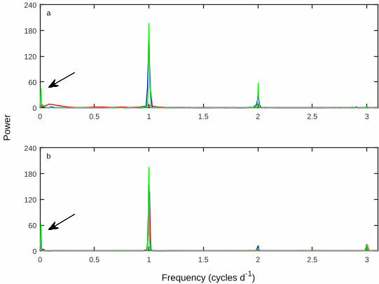
The magnitude of the diel trend appeared to be much greater than that of the lunar trend. 288
Indeed, at Kahekili, the reef with the strongest lunar trend, diel periodicity was approximately 289
four times stronger than lunar periodicity at both low and high frequencies (Fig. 8). The excess 290
strength of the diel trend was even greater for other reefs. 291
The strength of the diel trend in sound production on a given reef—defined here as the 292
area under the curve at dusk and dawn in each frequency band by month—was related to the 293
biological attributes of that reef (Fig. 9). At low frequencies, soniferous fish abundance was 294
positively correlated with the strength of the diel trend in October 2015 (Fig. 9c), but 295
relationships to coral cover and rugosity were not significant (Fig. 9a-b). At high frequencies, 296
positive correlations between coral cover and the strength of the diel trend were evident for all 297
survey periods except January 2016 (Fig. 9e). However, there appeared to be no relationships 298
between the strength of the diel trend at high frequencies and rugosity (Fig. 9d) or soniferous fish 299
abundance (Fig. 9f). 300
301
Discussion 302
The goal of this study was to better understand the drivers of biological sound production 303
on coral reefs and the extent to which acoustic records reflect fundamental ecological parameters 304
such as coral cover and reef fish biodiversity. Results from integrating the magnitude of the 305
crepuscular increase in biological sound production indicated that low-frequency sound levels, 306
driven by fish calling activity, were related to fish abundance. High-frequency levels, indicative 307
of snapping shrimp sounds, were related to coral cover. These data underscore the significance of 308

15
diel periodicity and further support the need to consider time of day when making recordings of 309
coral-reef soundscapes. 310
This study presents a new method of characterizing coral-reef soundscapes, using both 311
the patterns of biological activity (diel trends) and acoustic parameters directly related to the 312
frequencies of interest (sound pressure in the fish and snapping shrimp bands). In previous work, 313
the magnitude of the diel trend was computed by taking the difference between the dawn or dusk 314
peak in sound level and a low point at midnight (Kaplan et al. 2015). While that crude measure 315
also suggested links between biota and the soundscape, the approach was limited because of a 316
relatively low sample rate. Furthermore, by sampling only a maximum and a minimum for each 317
measurement, these results may have been more susceptible to influence by outliers. In the 318
present study, observations were made for 16 months on a 10% duty cycle that provided 319
recordings every 5 min. This long-term and fine-scale assessment of the magnitude of diel 320
periodicity allowed for the area under the curve to be integrated, offering a more robust measure 321
of crepuscular ecological trends. 322
Comparisons to physical parameters 323
Rugosity did not appear to relate to acoustic data in either frequency band. This is perhaps a 324
surprising result, given that other work has identified links between rugosity and fish density 325
(e.g., McCormick 1994), and it may have been anticipated that greater rugosity values would be 326
suggestive of more habitat for snapping shrimp and even fishes. While there was no linear 327
correlation, the strength of the low-frequency diel trend did peak at several reefs of mid-level 328
rugosity. These reefs also tended to have higher fish abundance. While speculative, this may 329
indicate that reefs whose rugosity is driven largely by coral cover and not rock formations (i.e., 330

16
reefs with intermediate rugosity) may be associated with higher fish abundance and greater diel 331
trend strengths. 332
Wind speed also did not appear to relate to acoustic data; however, such relationships 333
have been identified in other studies (e.g., Staaterman et al. 2014). This divergence could be 334
because wind speed data were obtained from a buoy in Kahului Harbor, near but not directly 335
adjacent to any of the recording sites. Alternatively, these reefs, many of which were close to 336
shore, may have been somewhat protected from the wind, which would suggest that soundscape 337
parameters were influenced by other factors. 338
Temperature did correlate significantly and positively with the high-frequency sound 339
levels of the snapping shrimp band, suggesting a relationship between snapping activity and local 340
temperature. The magnitude of this relationship varied among reefs, indicating that reef-specific 341
habitats may influence this relationship. This correlation between shrimp behavior and 342
temperature is consistent with other coral and oyster reef studies (e.g., Kaplan et al. 2015; 343
Bohnenstiehl et al. 2016); however, the causal link between temperature and snapping shrimp 344
activity has yet to be fully elucidated. Further work should investigate the mechanistic or 345
physiological drivers of this relationship. As seas warm, sound production rates may increase in 346
this high-frequency band. The negative correlation noted at MM17 could be a result of early 347
arrival of humpback whale song in the fall months (i.e., before the December cutoff after which 348
low-frequency recordings were not considered). 349
Comparisons of visual and acoustic data 350
Reefs were selected to cover the broadest possible gradient in benthic cover and fish density. 351
While reefs did vary appreciably in benthic cover, fish species assemblages proved to be more 352
similar among reefs than was originally desired (Fig. 3c–d) Furthermore, visually observed reef 353

17
fish species assemblages varied within reefs among survey periods, despite relatively frequent 354
observations (every 4–5 months). These changes may reflect community dynamics but might 355
also be a limitation of this method. Visual surveys are only snapshots of the fish community at a 356
particular point in time. These communities may vary by time of day, season, settlement, or in 357
stochastic ways not captured by the surveys (e.g., Sale et al. 1984; Galzin 1987; Syms and Jones 358
2000). More frequent observations would provide a more comprehensive estimation of the 359
community variability. Nevertheless, if timed correctly, visual surveys can reveal rare and 360
potentially important events such as coral bleaching or pulses of abnormally high fish 361
abundance, such as that at MM17 in September 2014, when abundance of pennant butterflyfish 362
(Heniochus diphreutes) was uncharacteristically high. However, it is not yet clear whether 363
acoustic records reveal such short-term changes. While acoustic data clearly identify temporal 364
cycles on diel, lunar, and seasonal scales, additional replications would be needed to determine 365
whether soundscape data have the resolution needed to identify transient ecological phenomena 366
such as bleaching events. 367
The changes over time reflected in these visual and acoustic data underscore how short-368
term observations (in both visual and acoustic data sets) may not generally be representative of 369
reef dynamics. Because there was no clear indication of how fast community changes took place, 370
care was taken to relate visual survey data to acoustic data only in months where the two datasets 371
overlapped. 372
Diel and lunar periodicity in SPL, which has been extensively described elsewhere 373
(Staaterman et al. 2014; Kaplan et al. 2015), was also evident here in both frequency bands at all 374
reefs. The exception was MM17, the sandy control site, where only limited and low-amplitude 375
variability was evident. Diel periodicity was notable, appeared to be much greater in magnitude 376

18
than lunar periodicity (Fig. 8), and may reflect the diversity of fish acoustic behaviors on these 377
reefs. 378
Sound levels in the low-frequency band were highest during the new moon periods and 379
lowest during the full moon. Larval fish settlement generally occurs during the new moon 380
(D'Alessandro et al. 2007) and is often lowest during the full moon, supporting the hypothesis 381
that sound may play a role as a settlement cue (e.g., Simpson et al. 2005). Less is known about 382
snapping shrimp behavior, which remains an area ripe for further investigation. 383
Notably, the strength of the diel trend provides a new means to assess coral-reef 384
soundscapes and the activity of the local biological community. The low-frequency fish-band 385
diel trend values tended to increase with soniferous fish abundance (Fig. 9), although these 386
correlations were variable and not always significant. This may be because an asymptote of 387
soniferous fish abundance was reached on these reefs. However, this variability is reflective of 388
reef environments which, as noted earlier, are not rigidly stable communities but areas in flux 389
(Sale et al. 1984; Meyer and Schultz 1985; Shulman 1985; Galzin 1987; Syms and Jones 2000). 390
High-frequency diel trend values increased with percentage coral cover, suggesting that snapping 391
shrimp activity may correlate with benthic cover. 392
In conclusion, the results presented here broadly characterize the soundscapes of these 393
study reefs. Overall, this study demonstrates that, despite the considerable variability in 394
biological sound production within and among reefs, the magnitude of the diel trend in sound 395
production was related at low frequencies to fish density and at high frequencies to coral cover. 396
Thus, while inverse prediction of species assemblages using the analysis techniques employed 397
here was not possible, acoustic recordings do provide a good indicator of community-level sound 398
production and how it changes over time. 399

19
400
Acknowledgements 401
Funding for this research was provided by the PADI Foundation, the WHOI Access To The Sea 402
initiative and Ocean Life Institute, and the National Science Foundation grant OCE-1536782. 403
We thank Lee James and Meagan Jones for generously providing vessel support. This research 404
benefited from helpful analysis advice from David Mann and Andy Solow and comments from 405
three anonymous reviewers. Alessandro Bocconcelli, Steve Faluotico, Merra Howe, Jim Partan, 406
Laela Sayigh, Russell Sparks, and Darla White provided engineering and technical assistance in 407
the field. This work was permitted by the Hawaii Department of Land and Natural Resources 408
(SAP 2015-29 and Special Use Permit 95132). 409
410
References 411
Au WWL, Banks K (1998) The acoustics of the snapping shrimp Synalpheus parneomeris in 412 Kaneohe Bay. J Acoust Soc Am 103:41–47 413
Au WW, Mobley J, Burgess WC, Lammers MO, Nachtigall PE (2000) Seasonal and diurnal 414 trends of chorusing humpback whales wintering in waters off western Maui. Mar Mam 415 Sci 16:530–544 416
Bertucci F, Parmentier E, Lecellier G, Hawkins AD, Lecchini D (2016) Acoustic indices provide 417 information on the status of coral reefs: an example from Moorea Island in the South 418 Pacific. Sci Rep 6:33326 419
Bohnenstiehl DR, Lillis A, Eggleston DB (2016) The curious acoustic behavior of estuarine 420 snapping shrimp: temporal patterns of snapping shrimp sound in sub-tidal oyster reef 421 habitat. PLoS One 11:e0143691 422
D'Alessandro E, Sponaugle S, Lee T (2007) Patterns and processes of larval fish supply to the 423 coral reefs of the upper Florida Keys. Mar Ecol Prog Ser 331:85–100 424
Friedlander AM, Brown EK, Jokiel PL, Smith WR, Rodgers KS (2003) Effects of habitat, wave 425 exposure, and marine protected area status on coral reef fish assemblages in the Hawaiian 426 archipelago. Coral Reefs 22:291–305 427
Galzin R (1987) Structure of fish communities of French Polynesian coral reefs. II. Temporal 428 scales. Mar Ecol Prog Ser 41:137–145 429
Kaplan MB, Mooney TA (2015) Ambient noise and temporal patterns of boat activity in the US 430 Virgin Islands National Park. Mar Pollut Bull 98:221–228 431
20
Kaplan MB, Mooney TA, Partan J, Solow AR (2015) Coral reef species assemblages are 432 associated with ambient soundscapes. Mar Ecol Prog Ser 533:93–107 433
Komyakova V, Munday PL, Jones GP (2013) Relative importance of coral cover, habitat 434 complexity and diversity in determining the structure of reef fish communities. PLoS One 435 8:e83178 436
Lammers MO, Brainard RE, Au WW, Mooney TA, Wong KB (2008) An ecological acoustic 437 recorder (EAR) for long-term monitoring of biological and anthropogenic sounds on 438 coral reefs and other marine habitats. J Acoust Soc Am 123:1720–1728 439
McCormick MI (1994) Comparison of field methods for measuring surface topography and their 440 associations with a tropical reef fish assemblage. Mar Ecol Prog Ser 112:87–96 441
Messmer V, Jones GP, Munday PL, Holbrook SJ, Schmitt RJ, Brooks A (2011) Habitat 442 biodiversity as a determinant of fish community structure on coral reefs. Ecology 443 92:2285–2298 444
Meyer JL, Schultz ET (1985) Migrating haemulid fishes as a source of nutrients and organic 445 matter on coral reefs. Limnol Oceanogr 30:146–156 446
Nedelec SL, Radford AN, Simpson SD, Nedelec B, Lecchini D, Mills SC (2014) Anthropogenic 447 noise playback impairs embryonic development and increases mortality in a marine 448 invertebrate. Sci Rep 4:5891 449
Nedelec SL, Simpson SD, Holderied M, Radford AN, Lecellier G, Radford C, Lecchini D (2015) 450 Soundscapes and living communities in coral reefs: temporal and spatial variation. Mar 451 Ecol Prog Ser 524:125–135 452
Parks SE, Miksis-Olds JL, Denes SL (2014) Assessing marine ecosystem acoustic diversity 453 across ocean basins. Ecol Inform 21:81–88 454
Parravicini V, Kulbicki M, Bellwood DR, Friedlander AM, Arias-Gonzalez JE, Chabanet P, 455 Floeter SR, Myers R, Vigliola L, D’Agata S, Mouillot D (2013) Global patterns and 456 predictors of tropical reef fish species richness. Ecography 36:1254–1262 457
Radford CA, Stanley JA, Jeffs AG (2014) Adjacent coral reef habitats produce different 458 underwater sound signatures. Mar Ecol Prog Ser 505:19–28 459
Radford CA, Jeffs AG, Tindle CT, Montgomery JC (2008) Temporal patterns in ambient noise 460 of biological origin from a shallow water temperate reef. Oecologia 156:921–929 461
Sale P, Doherty P, Eckert G, Douglas W, Ferrell D (1984) Large scale spatial and temporal 462 variation in recruitment to fish populations on coral reefs. Oecologia 64:191–198 463
Shulman MJ (1985) Recruitment of coral reef fishes: effects of distribution of predators and 464 shelter. Ecology 66:1056–1066 465
Simpson SD, Meekan M, Montgomery J, McCauley R, Jeffs A (2005) Homeward sound. 466 Science 308:221 467
Simpson SD, Radford AN, Nedelec SL, Ferrari MC, Chivers DP, McCormick MI, Meekan MG 468 (2016) Anthropogenic noise increases fish mortality by predation. Nat Commun 7:10544 469
Staaterman E, Paris CB, DeFerrari HA, Mann DA, Rice AN, D’Alessandro EK (2014) Celestial 470 patterns in marine soundscapes. Mar Ecol Prog Ser 508:17–32 471
Staaterman E, Ogburn MB, Altieri AH, Brandl SJ, Whippo R, Seemann J, Goodison M, Duffy 472 JE (2017) Bioacoustic measurements complement visual biodiversity surveys: 473 preliminary evidence from four shallow marine habitats. Mar Ecol Prog Ser 575:207–215 474
Syms C, Jones GP (2000) Disturbance, habitat structure, and the dynamics of a coral‐reef fish 475 community. Ecology 81:2714–2729 476
21
Tricas TC, Boyle KS (2014) Acoustic behaviors in Hawaiian coral reef fish communities. Mar 477 Ecol Prog Ser 511:1–16 478
Williams ID, Baum JK, Heenan A, Hanson KM, Nadon MO, Brainard RE (2015) Human, 479 oceanographic and habitat drivers of central and western Pacific coral reef fish 480 assemblages. PLoS One 10:e0120516 481
482
Figure captions 483
Fig. 1 a Map depicting the location of the seven study sites in Maui, Hawaii. b An ecological 484
acoustic recorder deployed at Olowalu 485
Fig. 2 Visual survey results by reef (ordered by low to high coral cover as recorded in the first 486
survey) and survey period (September 2014, February/March 2015, October 2015, January 487
2016). a Benthic cover, b abundance of soniferous and other fish, c fish species richness. Data on 488
sound-producing species were obtained from Tricas and Boyle (2014). CCA: crustose coralline 489
algae; TA: turf algae 490
Fig. 3 a Relationship between number of soniferous fish individuals (small: open circles; large: 491
filled circles) and live, unbleached coral cover. b Relationship between number of soniferous 492
fish species and live, unbleached coral cover. Non-metric multidimensional scaling (MDS) plots 493
of Bray–Curtis dissimilarity values for c soniferous and d all fishes. Results from all four visual 494
survey periods are included, and, for the MDS plots, are stratified by sampling period (circles: 495
September 2014; diamonds: February 2015; squares: October 2015; pentagons: January 2016) 496
Fig. 4 Daily average sound pressure level (SPL) in a low-frequency and b high-frequency bands 497
for the duration of the study at each reef 498
Fig. 5 Linear regression lines of daily average water temperature and sound pressure level (SPL) 499
at a low and b high frequencies across the study reefs (only significant correlations are shown). 500
Equations of the lines, evaluations of fit, and significance levels are in electronic supplementary 501
material Figs. S3, S4. 502

22
Fig. 6 Boxplots representing a low-frequency and b high-frequency sound pressure level (SPL) 503
at Kahekili during the new moon (black) first/last quarter (purple), and full moon (green) at four 504
times of day 505
Fig. 7 Median sound pressure level (SPL) (25–75 percentiles) at a low frequency and b high 506
frequency for each reef by hour of the day. Orange shading indicates dawn and blue shading 507
indicates dusk 508
Fig. 8 Fourier transforms depicting the magnitude of periodicity in sound pressure level (SPL) at 509
a low and b high frequencies for Kahekili. Colors represent individual deployment periods 510
Fig. 9 Strength of diel trend at a, b, c low frequency and d, e, f high frequency by month and reef 511
with associated rugosity (a, d), coral cover (bleached and unbleached) (b, e), and fish abundance 512
(c, f). Lines of best fit were plotted only when significant relationships were identified (grey 513
lines; see Table 3 for equations of the lines and evaluation of fit). Circles: September 2014; 514
diamonds: February 2015; squares: October 2015; pentagons: January 2016 515


MM17 Honolua Ahihi Kahekili Red Hill Olowalu Molokini0
50
100P
erce
nt c
over a
Live coral Bleached coral Macroalgae CCA TA Other
MM17 Honolua Ahihi Kahekili Red Hill Olowalu Molokini0
200
400
600
Num
ber
of fi
sh bSoniferous Other
MM17 Honolua Ahihi Kahekili Red Hill Olowalu Molokini
Reef
0
20
40
60
Obs
erve
d nu
mbe
rof
spe
cies
c

Live coral cover (%)
Dimension 1
-0.5 0 0.5 1-0.1
0
0.1
0.2
0.3d
-0.5 0 0.5 1-0.15
-0.1
-0.05
0
0.05
0.1
0.15
Dim
ensi
on 2
c
AHIHI HONOLUA KAHEKILI MM17 MOLOKINI OLOWALU RED HILL
0 20 40 60 80 1000
50
100
150
200
250
300
350
Num
ber
of s
onife
rous
fish
indi
vidu
als
a
0 20 40 60 80 1000
10
20
30
40
50
60
Num
ber
of s
onife
rous
spe
cies
b

10/14 01/15 04/15 07/15 10/15 01/1690
95
100
105
110
115
120
125S
PL rm
s 50-
1200
Hz
(dB
re
1 μ
Pa)
a
10/14 01/15 04/15 07/15 10/15 01/16
Date
105
110
115
120
125
SP
L rms 1
.8-2
0.5
kHz
(dB
re
1 μ
Pa)
b
AHIHIHONOLUAKAHEKILIMM17
MOLOKINIOLOWALURED HILL

Temperature (°C)
AHIHI HONOLUA KAHEKILI MM17 MOLOKINI RED HILL
22 24 26 28 30106
108
110
112
114
116
118
120
122
SP
L rms 1
.8-2
0.5
kHz
(dB
re
1 μ
Pa)
b
24 26 28 3092
93
94
95
96
97
98
99
100
101
102
SP
L rms 5
0-12
00 H
z (d
B r
e 1 μ
Pa)
a


Pow
er
Frequency (cycles d-1)
0 0.5 1 1.5 2 2.5 30
60
120
180
240a
0 0.5 1 1.5 2 2.5 30
60
120
180
240b

1 1.1 1.2 1.3 1.4 1.5
Rugosity
80
120
160
200
240
Low
-fre
quen
cy s
tren
gth
of d
iel t
rend
(dB
)
a
0 20 40 60 80 100
Coral cover (%)
80
120
160
200
240 b
0 100 200 300 400
Soniferous fish abundance (n)
80
120
160
200
240 c
1 1.1 1.2 1.3 1.4 1.5
Rugosity
50
100
150
200
250
Hig
h-fr
eque
ncy
stre
ngth
of d
iel t
rend
(dB
)
d
0 20 40 60 80 100
Coral cover (%)
50
100
150
200
250 e
0 100 200 300 400
Soniferous fish abundance (n)
50
100
150
200
250 f
AHIHI HONOLUA KAHEKILI MM17 MOLOKINI OLOWALU RED HILL