Embed Size (px)
Citation preview
5 © 2016 Cengage Learning®. May not be scanned, copied or duplicated, or posted to a publicly accessible website, in whole or in part.
2. MATLAB Basics
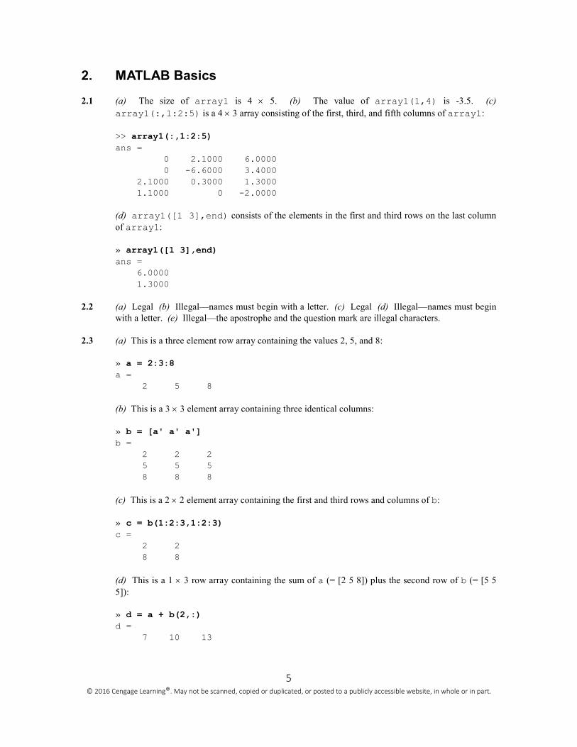
2.1 (a) The size of array1 is 4 × 5. (b) The value of array1(1,4) is -3.5. (c)
array1(:,1:2:5) is a 4 × 3 array consisting of the first, third, and fifth columns of array1:
>> array1(:,1:2:5)
ans =
0 2.1000 6.0000
0 -6.6000 3.4000
2.1000 0.3000 1.3000
1.1000 0 -2.0000
(d) array1([1 3],end) consists of the elements in the first and third rows on the last column
of array1:
» array1([1 3],end)
ans =
6.0000
1.3000
2.2 (a) Legal (b) Illegal—names must begin with a letter. (c) Legal (d) Illegal—names must begin
with a letter. (e) Illegal—the apostrophe and the question mark are illegal characters.
2.3 (a) This is a three element row array containing the values 2, 5, and 8:
» a = 2:3:8
a =
2 5 8
(b) This is a 3 × 3 element array containing three identical columns:
» b = [a' a' a']
b =
2 2 2
5 5 5
8 8 8
(c) This is a 2 × 2 element array containing the first and third rows and columns of b:
» c = b(1:2:3,1:2:3)
c =
2 2
8 8
(d) This is a 1 × 3 row array containing the sum of a (= [2 5 8]) plus the second row of b (= [5 5
5]):
» d = a + b(2,:)
d =
7 10 13
6 © 2016 Cengage Learning®. May not be scanned, copied or duplicated, or posted to a publicly accessible website, in whole or in part.
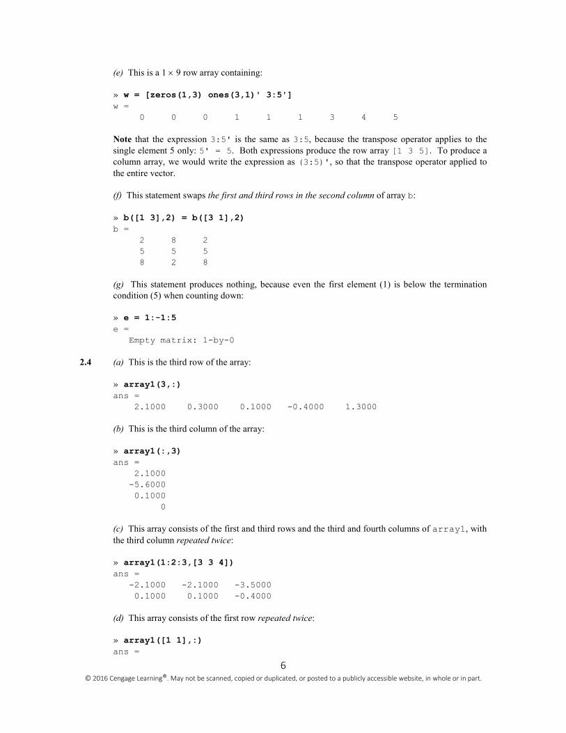
(e) This is a 1 × 9 row array containing:
» w = [zeros(1,3) ones(3,1)' 3:5']
w =
0 0 0 1 1 1 3 4 5
Note that the expression 3:5' is the same as 3:5, because the transpose operator applies to the
single element 5 only: 5' = 5. Both expressions produce the row array [1 3 5]. To produce a
column array, we would write the expression as (3:5)', so that the transpose operator applied to
the entire vector.
(f) This statement swaps the first and third rows in the second column of array b:
» b([1 3],2) = b([3 1],2)
b =
2 8 2
5 5 5
8 2 8
(g) This statement produces nothing, because even the first element (1) is below the termination
condition (5) when counting down:
» e = 1:-1:5
e =
Empty matrix: 1-by-0
2.4 (a) This is the third row of the array:
» array1(3,:)
ans =
2.1000 0.3000 0.1000 -0.4000 1.3000
(b) This is the third column of the array:
» array1(:,3)
ans =
2.1000
-5.6000
0.1000
0
(c) This array consists of the first and third rows and the third and fourth columns of array1, with
the third column repeated twice:
» array1(1:2:3,[3 3 4])
ans =
-2.1000 -2.1000 -3.5000
0.1000 0.1000 -0.4000
(d) This array consists of the first row repeated twice:
» array1([1 1],:)
ans =
7 © 2016 Cengage Learning®. May not be scanned, copied or duplicated, or posted to a publicly accessible website, in whole or in part.
1.1000 0 -2.1000 -3.5000 6.0000
1.1000 0 -2.1000 -3.5000 6.0000
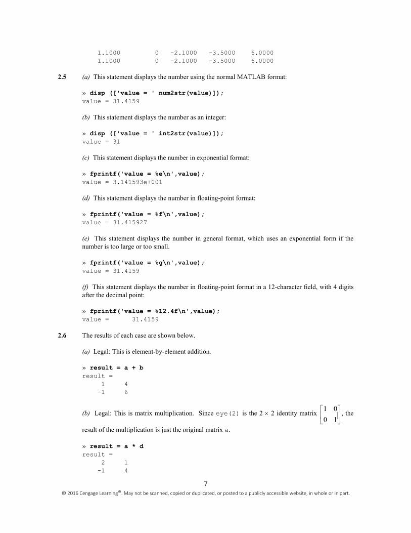
2.5 (a) This statement displays the number using the normal MATLAB format:
» disp (['value = ' num2str(value)]);
value = 31.4159
(b) This statement displays the number as an integer:
» disp (['value = ' int2str(value)]);
value = 31
(c) This statement displays the number in exponential format:
» fprintf('value = %e\n',value);
value = 3.141593e+001
(d) This statement displays the number in floating-point format:
» fprintf('value = %f\n',value);
value = 31.415927
(e) This statement displays the number in general format, which uses an exponential form if the
number is too large or too small.
» fprintf('value = %g\n',value);
value = 31.4159
(f) This statement displays the number in floating-point format in a 12-character field, with 4 digits
after the decimal point:
» fprintf('value = %12.4f\n',value);
value = 31.4159
2.6 The results of each case are shown below.
(a) Legal: This is element-by-element addition.
» result = a + b
result =
1 4
-1 6
(b) Legal: This is matrix multiplication. Since eye(2) is the 2 × 2 identity matrix 1 0
0 1
, the
result of the multiplication is just the original matrix a.
» result = a * d
result =
2 1
-1 4
8 © 2016 Cengage Learning®. May not be scanned, copied or duplicated, or posted to a publicly accessible website, in whole or in part.
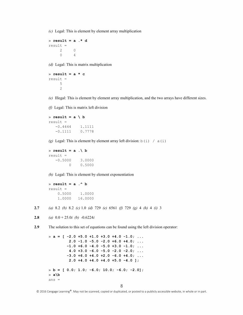
(c) Legal: This is element by element array multiplication
» result = a .* d
result =
2 0
0 4
(d) Legal: This is matrix multiplication
» result = a * c
result =
5
2
(e) Illegal: This is element by element array multiplication, and the two arrays have different sizes.
(f) Legal: This is matrix left division
» result = a \ b
result =
-0.4444 1.1111
-0.1111 0.7778
(g) Legal: This is element by element array left division: b(i) / a(i)
» result = a .\ b
result =
-0.5000 3.0000
0 0.5000
(h) Legal: This is element by element exponentiation
» result = a .^ b
result =
0.5000 1.0000
1.0000 16.0000
2.7 (a) 8.2 (b) 8.2 (c) 1.0 (d) 729 (e) 6561 (f) 729 (g) 4 (h) 4 (i) 3
2.8 (a) 0.0 + 25.0i (b) -0.6224i
2.9 The solution to this set of equations can be found using the left division operator:
» a = [ -2.0 +5.0 +1.0 +3.0 +4.0 -1.0; ...
2.0 -1.0 -5.0 -2.0 +6.0 +4.0; ...
-1.0 +6.0 -4.0 -5.0 +3.0 -1.0; ...
4.0 +3.0 -6.0 -5.0 -2.0 -2.0; ...
-3.0 +6.0 +4.0 +2.0 -6.0 +4.0; ...
2.0 +4.0 +4.0 +4.0 +5.0 -4.0 ];
» b = [ 0.0; 1.0; -6.0; 10.0; -6.0; -2.0];
» a\b
ans =
9 © 2016 Cengage Learning®. May not be scanned, copied or duplicated, or posted to a publicly accessible website, in whole or in part.
0.6626
-0.1326
-3.0137
2.8355
-1.0852
-0.8360
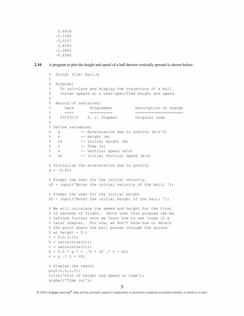
2.10 A program to plot the height and speed of a ball thrown vertically upward is shown below:
% Script file: ball.m
%
% Purpose:
% To calculate and display the trajectory of a ball
% thrown upward at a user-specified height and speed.
%
% Record of revisions:
% Date Programmer Description of change
% ==== ========== =====================
% 03/03/15 S. J. Chapman Original code
%
% Define variables:
% g -- Acceleration due to gravity (m/s^2)
% h -- Height (m)
% h0 -- Initial height (m)
% t -- Time (s)
% v -- Vertical Speed (m/s)
% v0 -- Initial Vertical Speed (m/s)
% Initialize the acceleration due to gravity
g = -9.81;
% Prompt the user for the initial velocity.
v0 = input('Enter the initial velocity of the ball: ');
% Prompt the user for the initial height
h0 = input('Enter the initial height of the ball: ');
% We will calculate the speed and height for the first
% 10 seconds of flight. (Note that this program can be
% refined further once we learn how to use loops in a
% later chapter. For now, we don't know how to detect
% the point where the ball passes through the ground
% at height = 0.)
t = 0:0.5:10;
h = zeros(size(t));
v = zeros(size(t));
h = 0.5 * g * t .^2 + v0 .* t + h0;
v = g .* t + v0;
% Display the result
plot(t,h,t,v);
title('Plot of height and speed vs time');
xlabel('Time (s)');
10 © 2016 Cengage Learning®. May not be scanned, copied or duplicated, or posted to a publicly accessible website, in whole or in part.
ylabel('Height (m) and Speed (m/s)');
legend('Height','Speed');
grid on;
When this program is executed, the results are:
» ball
Enter the initial velocity of the ball: 20
Enter the initial height of the ball: 10
2.11 A program to calculate the distance between two points in a Cartesian plane is shown below:
% Script file: dist2d.m
%
% Purpose:
% To calculate the distance between two points on a
% Cartesian plane.
%
% Record of revisions:
% Date Programmer Description of change
% ==== ========== =====================
% 03/03/15 S. J. Chapman Original code
%
% Define variables:
% dist -- Distance between points
% x1, y1 -- Point 1
% x2, y2 -- Point 2
11 © 2016 Cengage Learning®. May not be scanned, copied or duplicated, or posted to a publicly accessible website, in whole or in part.
% Prompt the user for the input points
x1 = input('Enter x1: ');
y1 = input('Enter y1: ');
x2 = input('Enter x2: ');
y2 = input('Enter y2: ');
% Calculate distance
dist = sqrt((x1-x2)^2 + (y1-y2)^2);
% Tell user
disp (['The distance is ' num2str(dist)]);
When this program is executed, the results are:
» dist2d
Enter x1: -3
Enter y1: 2
Enter x2: 6
Enter y2: -6
The distance is 10
2.12 A program to calculate the distance between two points in a Cartesian plane is shown below:
% Script file: dist3d.m
%
% Purpose:
% To calculate the distance between two points on a
% three-dimensional Cartesian plane.
%
% Record of revisions:
% Date Programmer Description of change
% ==== ========== =====================
% 03/03/15 S. J. Chapman Original code
%
% Define variables:
% dist -- Distance between points
% x1, y1, z1 -- Point 1
% x2, y2, z2 -- Point 2
% Prompt the user for the input points
x1 = input('Enter x1: ');
y1 = input('Enter y1: ');
z1 = input('Enter z1: ');
x2 = input('Enter x2: ');
y2 = input('Enter y2: ');
z2 = input('Enter z2: ');
% Calculate distance
dist = sqrt((x1-x2)^2 + (y1-y2)^2 + (z1-z2)^2);
% Tell user
disp (['The distance is ' num2str(dist)]);
12 © 2016 Cengage Learning®. May not be scanned, copied or duplicated, or posted to a publicly accessible website, in whole or in part.
When this program is executed, the results are:
» dist3d
Enter x1: -3
Enter y1: 2
Enter z1: 5
Enter x2: 3
Enter y2: -6
Enter z2: -5
The distance is 14.1421
2.13 A program to calculate power in dBm is shown below:
% Script file: decibel.m
%
% Purpose:
% To calculate the dBm corresponding to a user-supplied
% power in watts.
%
% Record of revisions:
% Date Programmer Description of change
% ==== ========== =====================
% 03/03/15 S. J. Chapman Original code
%
% Define variables:
% dBm -- Power in dBm
% pin -- Power in watts
% Prompt the user for the input power.
pin = input('Enter the power in watts: ');
% Calculate dBm
dBm = 10 * log10( pin / 1.0e-3 );
% Tell user
disp (['Power = ' num2str(dBm) ' dBm']);
When this program is executed, the results are:
» decibel
Enter the power in watts: 10
Power = 40 dBm » decibel
Enter the power in watts: 0.1
Power = 20 dBm
When this program is executed, the results are:
% Script file: db_plot.m
%
% Purpose:
% To plot power in watts vs power in dBm on a linear and
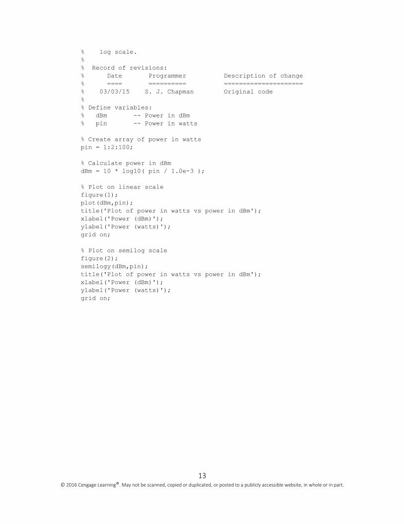
13 © 2016 Cengage Learning®. May not be scanned, copied or duplicated, or posted to a publicly accessible website, in whole or in part.
% log scale.
%
% Record of revisions:
% Date Programmer Description of change
% ==== ========== =====================
% 03/03/15 S. J. Chapman Original code
%
% Define variables:
% dBm -- Power in dBm
% pin -- Power in watts
% Create array of power in watts
pin = 1:2:100;
% Calculate power in dBm
dBm = 10 * log10( pin / 1.0e-3 );
% Plot on linear scale
figure(1);
plot(dBm,pin);
title('Plot of power in watts vs power in dBm');
xlabel('Power (dBm)');
ylabel('Power (watts)');
grid on;
% Plot on semilog scale
figure(2);
semilogy(dBm,pin);
title('Plot of power in watts vs power in dBm');
xlabel('Power (dBm)');
ylabel('Power (watts)');
grid on;
14 © 2016 Cengage Learning®. May not be scanned, copied or duplicated, or posted to a publicly accessible website, in whole or in part.
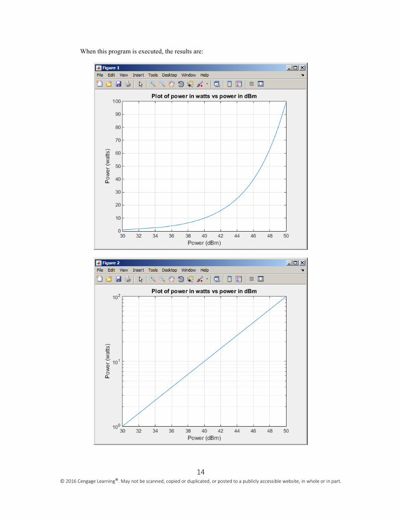
When this program is executed, the results are:
15 © 2016 Cengage Learning®. May not be scanned, copied or duplicated, or posted to a publicly accessible website, in whole or in part.
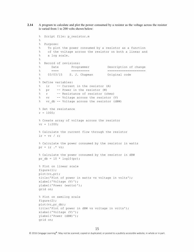
2.14 A program to calculate and plot the power consumed by a resistor as the voltage across the resistor
is varied from 1 to 200 volts shown below:
% Script file: p_resistor.m
%
% Purpose:
% To plot the power consumed by a resistor as a function
% of the voltage across the resistor on both a linear and
% a log scale.
%
% Record of revisions:
% Date Programmer Description of change
% ==== ========== =====================
% 03/03/15 S. J. Chapman Original code
%
% Define variables:
% ir -- Current in the resistor (A)
% pr -- Power in the resistor (W)
% r -- Resistance of resistor (ohms)
% vr -- Voltage across the resistor (V)
% vr_db -- Voltage across the resistor (dBW)
% Set the resistance
r = 1000;
% Create array of voltage across the resistor
vr = 1:200;
% Calculate the current flow through the resistor
ir = vr / r;
% Calculate the power consumed by the resistor in watts
pr = ir .* vr;
% Calculate the power consumed by the resistor in dBW
pr_db = 10 * log10(pr);
% Plot on linear scale
figure(1);
plot(vr,pr);
title('Plot of power in watts vs voltage in volts');
xlabel('Voltage (V)');
ylabel('Power (watts)');
grid on;
% Plot on semilog scale
figure(2);
plot(vr,pr_db);
title('Plot of power in dBW vs voltage in volts');
xlabel('Voltage (V)');
ylabel('Power (dBW)');
grid on;
16 © 2016 Cengage Learning®. May not be scanned, copied or duplicated, or posted to a publicly accessible website, in whole or in part.
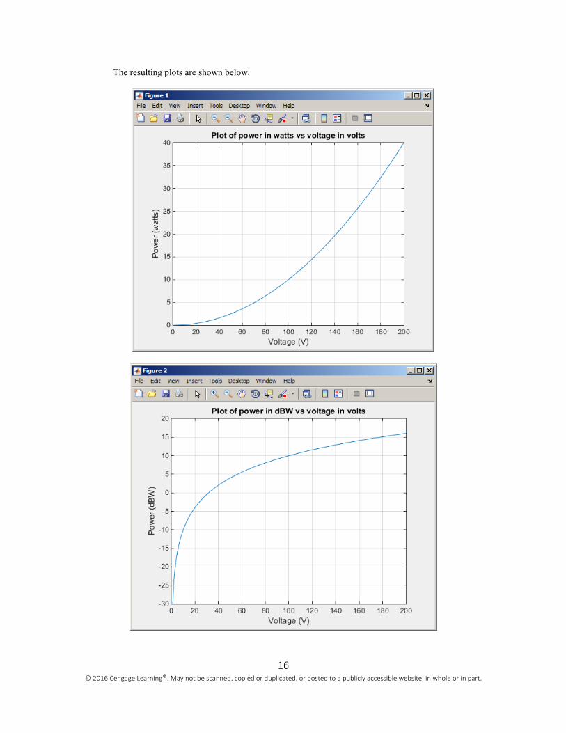
The resulting plots are shown below.
17 © 2016 Cengage Learning®. May not be scanned, copied or duplicated, or posted to a publicly accessible website, in whole or in part.
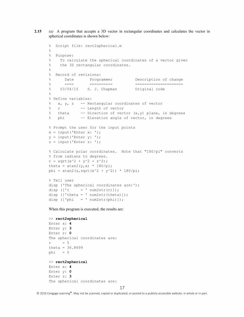
2.15 (a) A program that accepts a 3D vector in rectangular coordinates and calculates the vector in
spherical coordinates is shown below:
% Script file: rect2spherical.m
%
% Purpose:
% To calculate the spherical coordinates of a vector given
% the 3D rectangular coordinates.
%
% Record of revisions:
% Date Programmer Description of change
% ==== ========== =====================
% 03/04/15 S. J. Chapman Original code
%
% Define variables:
% x, y, z -- Rectangular coordinates of vector
% r -- Length of vector
% theta -- Direction of vector (x,y) plane, in degrees
% phi -- Elevation angle of vector, in degrees
% Prompt the user for the input points
x = input('Enter x: ');
y = input('Enter y: ');
z = input('Enter z: ');
% Calculate polar coordinates. Note that "180/pi" converts
% from radians to degrees.
r = sqrt(x^2 + y^2 + z^2);
theta = atan2(y,x) * 180/pi;
phi = atan2(z,sqrt(x^2 + y^2)) * 180/pi;
% Tell user
disp ('The spherical coordinates are:');
disp (['r = ' num2str(r)]);
disp (['theta = ' num2str(theta)]);
disp (['phi = ' num2str(phi)]);
When this program is executed, the results are:
>> rect2spherical
Enter x: 4
Enter y: 3
Enter z: 0
The spherical coordinates are:
r = 5
theta = 36.8699
phi = 0
>> rect2spherical
Enter x: 4
Enter y: 0
Enter z: 3
The spherical coordinates are:
18 © 2016 Cengage Learning®. May not be scanned, copied or duplicated, or posted to a publicly accessible website, in whole or in part.
r = 5
theta = 0
phi = 36.8699
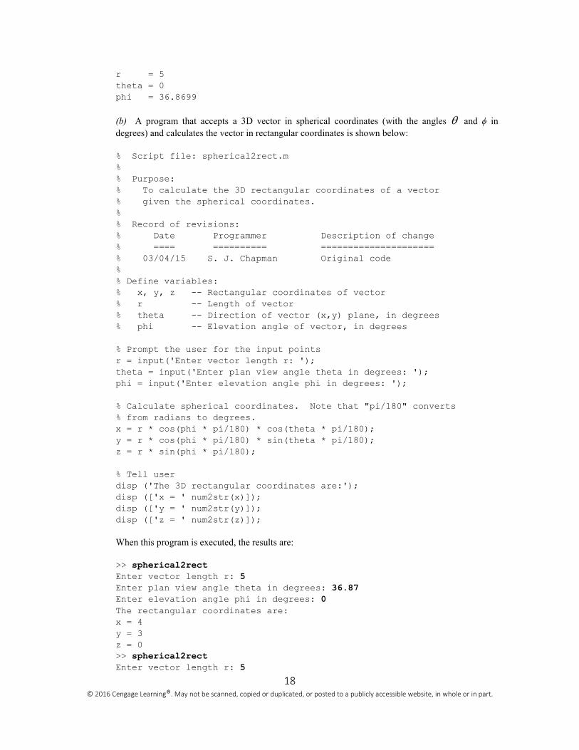
(b) A program that accepts a 3D vector in spherical coordinates (with the angles θ and ϕ in
degrees) and calculates the vector in rectangular coordinates is shown below:
% Script file: spherical2rect.m
%
% Purpose:
% To calculate the 3D rectangular coordinates of a vector
% given the spherical coordinates.
%
% Record of revisions:
% Date Programmer Description of change
% ==== ========== =====================
% 03/04/15 S. J. Chapman Original code
%
% Define variables:
% x, y, z -- Rectangular coordinates of vector
% r -- Length of vector
% theta -- Direction of vector (x,y) plane, in degrees
% phi -- Elevation angle of vector, in degrees
% Prompt the user for the input points
r = input('Enter vector length r: ');
theta = input('Enter plan view angle theta in degrees: ');
phi = input('Enter elevation angle phi in degrees: ');
% Calculate spherical coordinates. Note that "pi/180" converts
% from radians to degrees.
x = r * cos(phi * pi/180) * cos(theta * pi/180);
y = r * cos(phi * pi/180) * sin(theta * pi/180);
z = r * sin(phi * pi/180);
% Tell user
disp ('The 3D rectangular coordinates are:');
disp (['x = ' num2str(x)]);
disp (['y = ' num2str(y)]);
disp (['z = ' num2str(z)]);
When this program is executed, the results are:
>> spherical2rect
Enter vector length r: 5
Enter plan view angle theta in degrees: 36.87
Enter elevation angle phi in degrees: 0
The rectangular coordinates are:
x = 4
y = 3
z = 0 >> spherical2rect
Enter vector length r: 5
19 © 2016 Cengage Learning®. May not be scanned, copied or duplicated, or posted to a publicly accessible website, in whole or in part.
Enter plan view angle theta in degrees: 0
Enter elevation angle phi in degrees: 36.87
The rectangular coordinates are:
x = 4
y = 0
z = 3
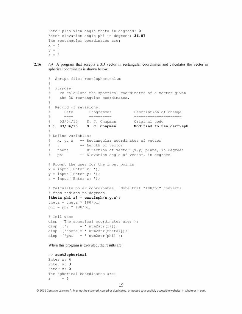
2.16 (a) A program that accepts a 3D vector in rectangular coordinates and calculates the vector in
spherical coordinates is shown below:
% Script file: rect2spherical.m
%
% Purpose:
% To calculate the spherical coordinates of a vector given
% the 3D rectangular coordinates.
%
% Record of revisions:
% Date Programmer Description of change
% ==== ========== =====================
% 03/04/15 S. J. Chapman Original code % 1. 03/04/15 S. J. Chapman Modified to use cart2sph
%
% Define variables:
% x, y, z -- Rectangular coordinates of vector
% r -- Length of vector
% theta -- Direction of vector (x,y) plane, in degrees
% phi -- Elevation angle of vector, in degrees
% Prompt the user for the input points
x = input('Enter x: ');
y = input('Enter y: ');
z = input('Enter z: ');
% Calculate polar coordinates. Note that "180/pi" converts
% from radians to degrees. [theta,phi,r] = cart2sph(x,y,z);
theta = theta * 180/pi;
phi = phi * 180/pi;
% Tell user
disp ('The spherical coordinates are:');
disp (['r = ' num2str(r)]);
disp (['theta = ' num2str(theta)]);
disp (['phi = ' num2str(phi)]);
When this program is executed, the results are:
>> rect2spherical
Enter x: 4
Enter y: 3
Enter z: 0
The spherical coordinates are:
r = 5
20 © 2016 Cengage Learning®. May not be scanned, copied or duplicated, or posted to a publicly accessible website, in whole or in part.
theta = 36.8699
phi = 0
>> rect2spherical
Enter x: 4
Enter y: 0
Enter z: 3
The spherical coordinates are:
r = 5
theta = 0
phi = 36.8699
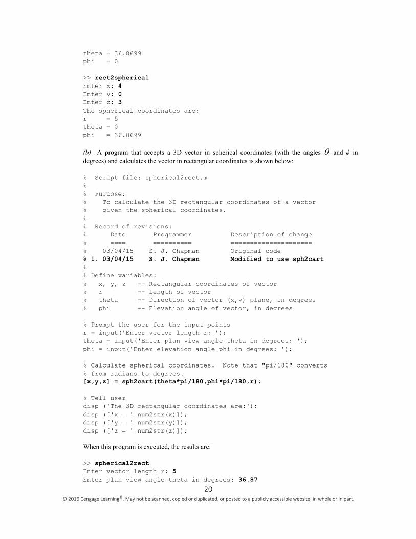
(b) A program that accepts a 3D vector in spherical coordinates (with the angles θ and ϕ in
degrees) and calculates the vector in rectangular coordinates is shown below:
% Script file: spherical2rect.m
%
% Purpose:
% To calculate the 3D rectangular coordinates of a vector
% given the spherical coordinates.
%
% Record of revisions:
% Date Programmer Description of change
% ==== ========== =====================
% 03/04/15 S. J. Chapman Original code % 1. 03/04/15 S. J. Chapman Modified to use sph2cart
%
% Define variables:
% x, y, z -- Rectangular coordinates of vector
% r -- Length of vector
% theta -- Direction of vector (x,y) plane, in degrees
% phi -- Elevation angle of vector, in degrees
% Prompt the user for the input points
r = input('Enter vector length r: ');
theta = input('Enter plan view angle theta in degrees: ');
phi = input('Enter elevation angle phi in degrees: ');
% Calculate spherical coordinates. Note that "pi/180" converts
% from radians to degrees. [x,y,z] = sph2cart(theta*pi/180,phi*pi/180,r);
% Tell user
disp ('The 3D rectangular coordinates are:');
disp (['x = ' num2str(x)]);
disp (['y = ' num2str(y)]);
disp (['z = ' num2str(z)]);
When this program is executed, the results are:
>> spherical2rect
Enter vector length r: 5
Enter plan view angle theta in degrees: 36.87
21 © 2016 Cengage Learning®. May not be scanned, copied or duplicated, or posted to a publicly accessible website, in whole or in part.
Enter elevation angle phi in degrees: 0
The rectangular coordinates are:
x = 4
y = 3
z = 0 >> spherical2rect
Enter vector length r: 5
Enter plan view angle theta in degrees: 0
Enter elevation angle phi in degrees: 36.87
The rectangular coordinates are:
x = 4
y = 0
z = 3
2.17 A program to calculate cosh(x) both from the definition and using the MATLAB intrinsic function is
shown below. Note that we are using fprintf to display the results, so that we can control the
number of digits displayed after the decimal point:
% Script file: cosh1.m
%
% Purpose:
% To calculate the hyperbolic cosine of x.
%
% Record of revisions:
% Date Programmer Description of change
% ==== ========== =====================
% 03/04/15 S. J. Chapman Original code
%
% Define variables:
% x -- Input value
% res1 -- cosh(x) from the definition
% res2 -- cosh(x) from the MATLAB function
% Prompt the user for the input power.
x = input('Enter x: ');
% Calculate cosh(x)
res1 = ( exp(x) + exp(-x) ) / 2;
res2 = cosh(x);
% Tell user
fprintf('Result from definition = %14.10f\n',res1);
fprintf('Result from function = %14.10f\n',res2);
When this program is executed, the results are:
» cosh1
Enter x: 3
Result from definition = 10.0676619958
Result from function = 10.0676619958
A program to plot cosh x is shown below:
22 © 2016 Cengage Learning®. May not be scanned, copied or duplicated, or posted to a publicly accessible website, in whole or in part.
% Script file: cosh_plot.m
%
% Purpose:
% To plot cosh x vs x.
%
% Record of revisions:
% Date Programmer Description of change
% ==== ========== =====================
% 03/04/15 S. J. Chapman Original code
%
% Define variables:
% x -- input values
% coshx -- cosh(x)
% Create array of power in input values
x = -3:0.1:3;
% Calculate cosh(x)
coshx = cosh(x);
% Plot on linear scale
plot(x,coshx);
title('Plot of cosh(x) vs x');
xlabel('x');
ylabel('cosh(x)');
grid on;
23 © 2016 Cengage Learning®. May not be scanned, copied or duplicated, or posted to a publicly accessible website, in whole or in part.
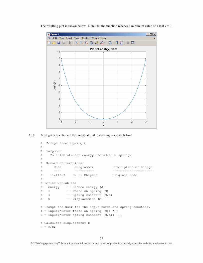
The resulting plot is shown below. Note that the function reaches a minimum value of 1.0 at x = 0.
2.18 A program to calculate the energy stored in a spring is shown below:
% Script file: spring.m
%
% Purpose:
% To calculate the energy stored in a spring.
%
% Record of revisions:
% Date Programmer Description of change
% ==== ========== =====================
% 11/14/07 S. J. Chapman Original code
%
% Define variables:
% energy -- Stored energy (J)
% f -- Force on spring (N)
% k -- Spring constant (N/m)
% x -- Displacement (m)
% Prompt the user for the input force and spring constant.
f = input('Enter force on spring (N): ');
k = input('Enter spring constant (N/m): ');
% Calculate displacement x
x = f/k;
24 © 2016 Cengage Learning®. May not be scanned, copied or duplicated, or posted to a publicly accessible website, in whole or in part.
% Calculate stored energy
energy = 0.5 * k * x^2;
% Tell user
fprintf('Displacement = %.3f meters\n',x);
fprintf('Stored energy = %.3f joules\n',energy);
When this program is executed, the results are as shown below. The second spring stores the most
energy.
» spring
Enter force on spring (N): 20
Enter spring constant (N/m): 200
Displacement = 0.100 meters
Stored energy = 1.000 joules » spring
Enter force on spring (N): 30
Enter spring constant (N/m): 250
Displacement = 0.120 meters
Stored energy = 1.800 joules » spring
Enter force on spring (N): 25
Enter spring constant (N/m): 300
Displacement = 0.083 meters
Stored energy = 1.042 joules » spring
Enter force on spring (N): 20
Enter spring constant (N/m): 800
Displacement = 0.050 meters
Stored energy = 0.500 joules
2.19 A program to calculate the resonant frequency of a radio is shown below:
% Script file: radio.m
%
% Purpose:
% To calculate the resonant frequency of a radio.
%
% Record of revisions:
% Date Programmer Description of change
% ==== ========== =====================
% 03/05/15 S. J. Chapman Original code
%
% Define variables:
% c -- Capacitance (F)
% freq -- Resonant frequency (Hz)
% l -- Inductance (H)
% Prompt the user for the input force and spring constant.
l = input('Enter inductance in henrys: ');
c = input('Enter capacitance in farads: ');
% Calculate resonant frequency
25 © 2016 Cengage Learning®. May not be scanned, copied or duplicated, or posted to a publicly accessible website, in whole or in part.
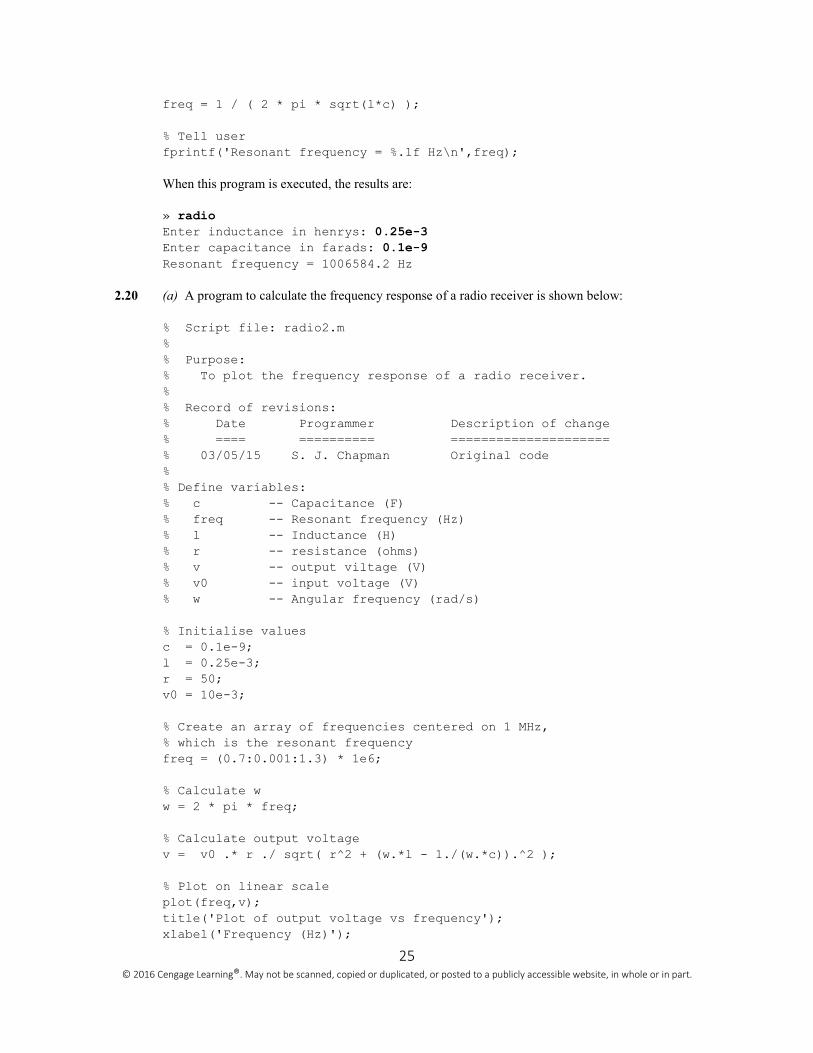
freq = 1 / ( 2 * pi * sqrt(l*c) );
% Tell user
fprintf('Resonant frequency = %.1f Hz\n',freq);
When this program is executed, the results are:
» radio
Enter inductance in henrys: 0.25e-3
Enter capacitance in farads: 0.1e-9
Resonant frequency = 1006584.2 Hz
2.20 (a) A program to calculate the frequency response of a radio receiver is shown below:
% Script file: radio2.m
%
% Purpose:
% To plot the frequency response of a radio receiver.
%
% Record of revisions:
% Date Programmer Description of change
% ==== ========== =====================
% 03/05/15 S. J. Chapman Original code
%
% Define variables:
% c -- Capacitance (F)
% freq -- Resonant frequency (Hz)
% l -- Inductance (H)
% r -- resistance (ohms)
% v -- output viltage (V)
% v0 -- input voltage (V)
% w -- Angular frequency (rad/s)
% Initialise values
c = 0.1e-9;
l = 0.25e-3;
r = 50;
v0 = 10e-3;
% Create an array of frequencies centered on 1 MHz,
% which is the resonant frequency
freq = (0.7:0.001:1.3) * 1e6;
% Calculate w
w = 2 * pi * freq;
% Calculate output voltage
v = v0 .* r ./ sqrt( r^2 + (w.*l - 1./(w.*c)).^2 );
% Plot on linear scale
plot(freq,v);
title('Plot of output voltage vs frequency');
xlabel('Frequency (Hz)');
26 © 2016 Cengage Learning®. May not be scanned, copied or duplicated, or posted to a publicly accessible website, in whole or in part.
ylabel('Voltage (V)');
grid on;
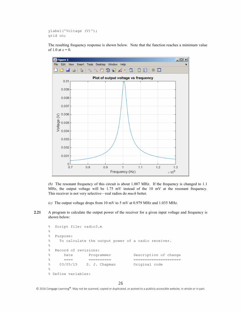
The resulting frequency response is shown below. Note that the function reaches a minimum value
of 1.0 at x = 0.
(b) The resonant frequency of this circuit is about 1.007 MHz. If the frequency is changed to 1.1
MHz, the output voltage will be 1.75 mV instead of the 10 mV at the resonant frequency.
This receiver is not very selective—real radios do much better.
(c) The output voltage drops from 10 mV to 5 mV at 0.979 MHz and 1.035 MHz.
2.21 A program to calculate the output power of the receiver for a given input voltage and frequency is
shown below:
% Script file: radio3.m
%
% Purpose:
% To calculate the output power of a radio receiver.
%
% Record of revisions:
% Date Programmer Description of change
% ==== ========== =====================
% 03/05/15 S. J. Chapman Original code
%
% Define variables:
27 © 2016 Cengage Learning®. May not be scanned, copied or duplicated, or posted to a publicly accessible website, in whole or in part.
% c -- Capacitance (F)
% freq -- Resonant frequency (Hz)
% l -- Inductance (H)
% r -- resistance (ohms)
% p -- output power (W)
% v -- output viltage (V)
% v0 -- input voltage (V)
% w -- Angular frequency (rad/s)
% Initialise values
c = 0.1e-9;
l = 0.25e-3;
r = 50;
% Get voltage and frequency
v0 = input('Enter voltage (V): ');
freq = input('Enter frequency (Hz): ');
% Calculate w
w = 2 * pi * freq;
% Calculate output voltage
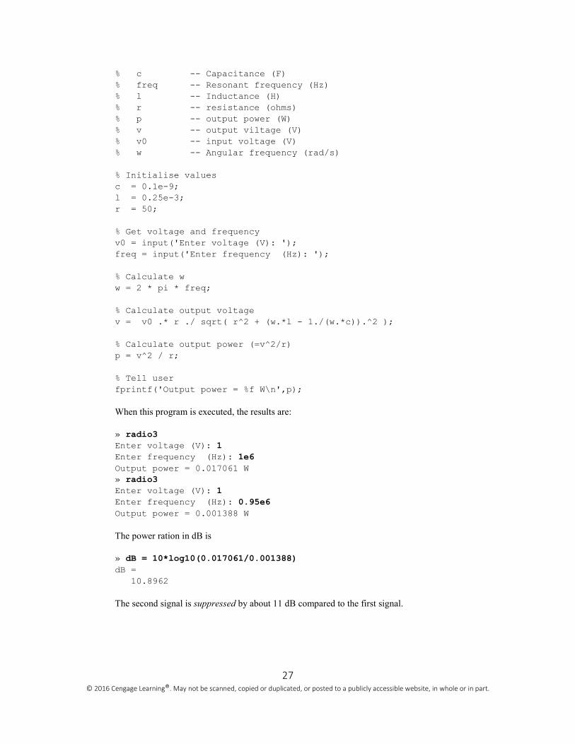
v = v0 .* r ./ sqrt( r^2 + (w.*l - 1./(w.*c)).^2 );
% Calculate output power (=v^2/r)
p = v^2 / r;
% Tell user
fprintf('Output power = %f W\n',p);
When this program is executed, the results are:
» radio3
Enter voltage (V): 1
Enter frequency (Hz): 1e6
Output power = 0.017061 W » radio3
Enter voltage (V): 1
Enter frequency (Hz): 0.95e6
Output power = 0.001388 W
The power ration in dB is
» dB = 10*log10(0.017061/0.001388)
dB =
10.8962
The second signal is suppressed by about 11 dB compared to the first signal.
28 © 2016 Cengage Learning®. May not be scanned, copied or duplicated, or posted to a publicly accessible website, in whole or in part.
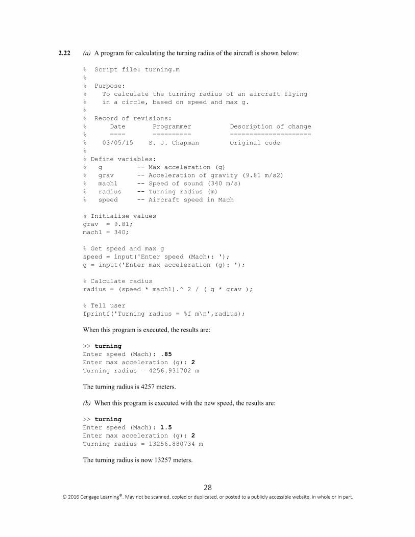
2.22 (a) A program for calculating the turning radius of the aircraft is shown below:
% Script file: turning.m
%
% Purpose:
% To calculate the turning radius of an aircraft flying
% in a circle, based on speed and max g.
%
% Record of revisions:
% Date Programmer Description of change
% ==== ========== =====================
% 03/05/15 S. J. Chapman Original code
%
% Define variables:
% g -- Max acceleration (g)
% grav -- Acceleration of gravity (9.81 m/s2)
% mach1 -- Speed of sound (340 m/s)
% radius -- Turning radius (m)
% speed -- Aircraft speed in Mach
% Initialise values
grav = 9.81;
mach1 = 340;
% Get speed and max g
speed = input('Enter speed (Mach): ');
g = input('Enter max acceleration (g): ');
% Calculate radius
radius = (speed * mach1).^ 2 / ( g * grav );
% Tell user
fprintf('Turning radius = %f m\n',radius);
When this program is executed, the results are:
>> turning
Enter speed (Mach): .85
Enter max acceleration (g): 2
Turning radius = 4256.931702 m
The turning radius is 4257 meters.
(b) When this program is executed with the new speed, the results are:
>> turning
Enter speed (Mach): 1.5
Enter max acceleration (g): 2
Turning radius = 13256.880734 m
The turning radius is now 13257 meters.

29 © 2016 Cengage Learning®. May not be scanned, copied or duplicated, or posted to a publicly accessible website, in whole or in part.
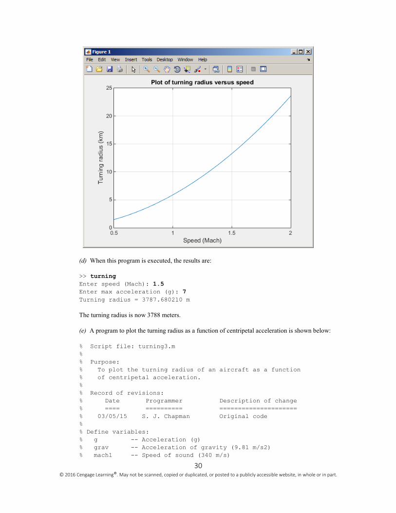
(c) A program to plot the turning radius as a function of speed for a constant max acceleration is
shown below:
% Script file: turning2.m
%
% Purpose:
% To plot the turning radius of an aircraft as a function
% of speed.
%
% Record of revisions:
% Date Programmer Description of change
% ==== ========== =====================
% 03/05/15 S. J. Chapman Original code
%
% Define variables:
% g -- Max acceleration (g)
% grav -- Acceleration of gravity (9.81 m/s2)
% mach1 -- Speed of sound (340 m/s)
% max_speed -- Maximum speed in Mach numbers
% min_speed -- Minimum speed in Mach numbers
% radius -- Turning radius (m)
% speed -- Aircraft speed in Mach
% Initialise values
grav = 9.81;
mach1 = 340;
% Get speed and max g
min_speed = input('Enter min speed (Mach): ');
max_speed = input('Enter min speed (Mach): ');
g = input('Enter max acceleration (g): ');
% Calculate range of speeds
speed = min_speed:(max_speed-min_speed)/20:max_speed;
% Calculate radius
radius = (speed * mach1).^ 2 / ( g * grav );
% Plot the turning radius versus speed
plot(speed,radius/1000);
title('Plot of turning radius versus speed');
xlabel('Speed (Mach)');
ylabel('Turning radius (km)');
grid on;
When this program is executed, the results are as shown below:
>> turning2
Enter min speed (Mach): 0.5
Enter min speed (Mach): 2.0
Enter max acceleration (g): 2
30 © 2016 Cengage Learning®. May not be scanned, copied or duplicated, or posted to a publicly accessible website, in whole or in part.
(d) When this program is executed, the results are:
>> turning
Enter speed (Mach): 1.5
Enter max acceleration (g): 7
Turning radius = 3787.680210 m
The turning radius is now 3788 meters.
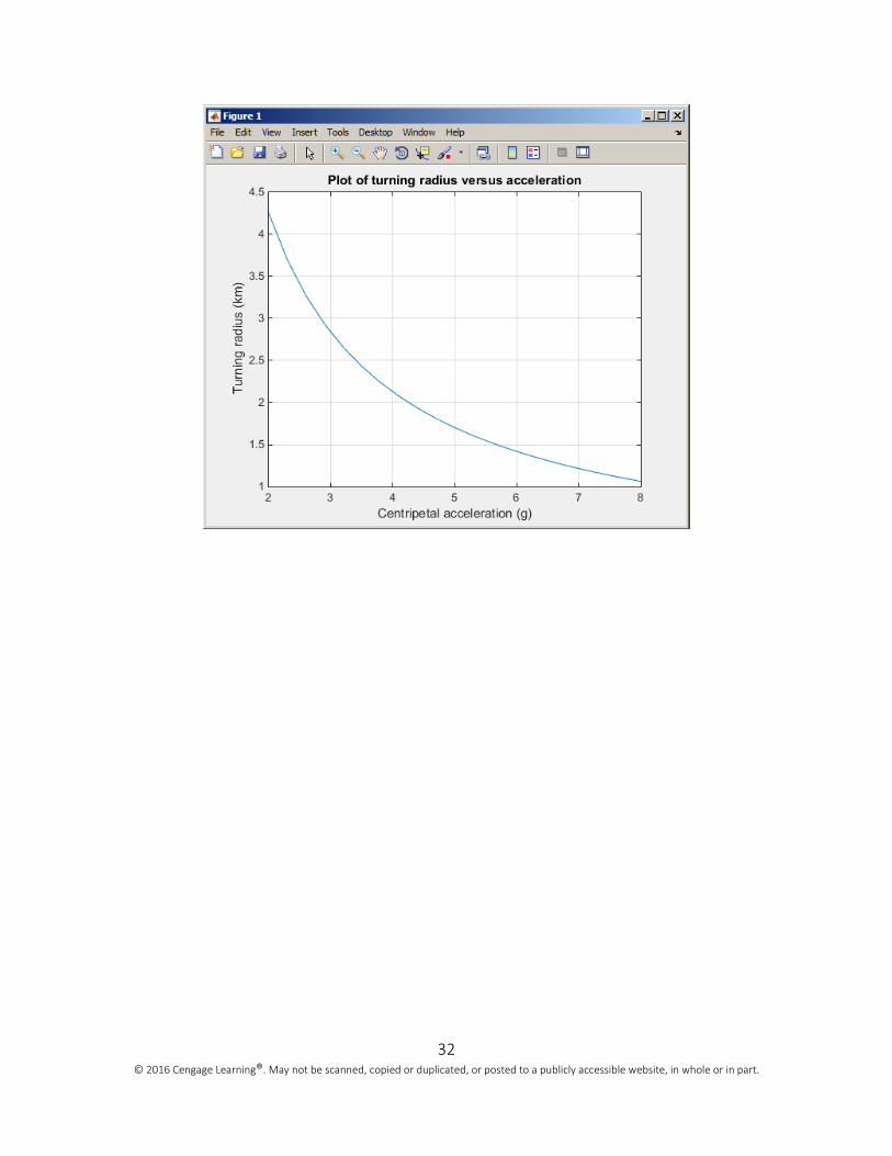
(e) A program to plot the turning radius as a function of centripetal acceleration is shown below:
% Script file: turning3.m
%
% Purpose:
% To plot the turning radius of an aircraft as a function
% of centripetal acceleration.
%
% Record of revisions:
% Date Programmer Description of change
% ==== ========== =====================
% 03/05/15 S. J. Chapman Original code
%
% Define variables:
% g -- Acceleration (g)
% grav -- Acceleration of gravity (9.81 m/s2)
% mach1 -- Speed of sound (340 m/s)
31 © 2016 Cengage Learning®. May not be scanned, copied or duplicated, or posted to a publicly accessible website, in whole or in part.
% max_g -- Maximum accleration in g's
% min_g -- Minimum accleration in g's
% radius -- Turning radius (m)
% speed -- Aircraft speed in Mach
% Initialise values
grav = 9.81;
mach1 = 340;
% Get speed and max g
speed = input('Enter speed (Mach): ');
min_g = input('Enter min acceleration (g): ');
max_g = input('Enter min acceleration (g): ');
% Calculate range of accelerations
g = min_g:(max_g-min_g)/20:max_g;
% Calculate radius
radius = (speed * mach1).^ 2 ./ ( g * grav );
% Plot the turning radius versus speed
plot(g,radius/1000);
title('Plot of turning radius versus acceleration');
xlabel('Centripetal acceleration (g)');
ylabel('Turning radius (km)');
grid on;
When this program is executed, the results are as shown below:
>> turning3
Enter speed (Mach): 0.85
Enter min acceleration (g): 2
Enter min acceleration (g): 8
32 © 2016 Cengage Learning®. May not be scanned, copied or duplicated, or posted to a publicly accessible website, in whole or in part.
1 © 2016 Cengage Learning Engineering. All Rights Reserved.
Chapter 2
MATLAB Basics
MATLAB Programming for Engineers, 5th edition Chapman
MATLAB Programming for Engineers, 5th edition Chapman
© 2016 Cengage Learning Engineering. All Rights Reserved. 2
Overview
∗ 2.1 Variables and Arrays
∗ 2.2 Creating and Initializing Variables in MATLAB
∗ 2.3 Multidimensional Arrays
∗ 2.4 Subarrays
∗ 2.5 Special Values
∗ 2.6 Displaying Output Data
∗ 2.7 Data Files
MATLAB Programming for Engineers, 5th edition Chapman
© 2016 Cengage Learning Engineering. All Rights Reserved. 3
Overview (continued)
∗ 2.8 Scalar and Array Operations
∗ 2.9 Hierarchy of Operations
2.10 Built-in MATLAB Functions
∗ 2.11 Introduction to Plotting
∗ 2.12 Examples (see text)
∗ 2.13 Debugging MATLAB Programs
∗ 2.14 Summary
MATLAB Programming for Engineers, 5th edition Chapman
© 2016 Cengage Learning Engineering. All Rights Reserved. 4
2.1 Variables and Arrays
∗ The fundamental unit of data in any MATLAB program is the array
∗ An array is a collection of data values organized into rows and columns and is known by a single name
∗ Arrays can be classified as either vectors or matrices
MATLAB Programming for Engineers, 5th edition Chapman
© 2016 Cengage Learning Engineering. All Rights Reserved. 5
More on Variables and Arrays
∗ Scalars are treated as arrays with only one row and one column
∗ The size of an array is given as # of rows by # of columns
∗ A MATLAB variable is a region of memory containing an array and is known by a user-specified name
MATLAB Programming for Engineers, 5th edition Chapman
© 2016 Cengage Learning Engineering. All Rights Reserved. 6
Introduction to Data Types
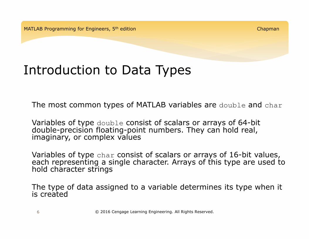
∗ The most common types of MATLAB variables are double and char
∗ Variables of type double consist of scalars or arrays of 64-bit double-precision floating-point numbers. They can hold real, imaginary, or complex values
∗ Variables of type char consist of scalars or arrays of 16-bit values, each representing a single character. Arrays of this type are used to hold character strings
∗ The type of data assigned to a variable determines its type when it is created
MATLAB Programming for Engineers, 5th edition Chapman
© 2016 Cengage Learning Engineering. All Rights Reserved. 7
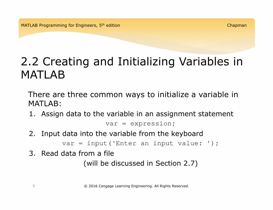
2.2 Creating and Initializing Variables in MATLAB
∗ There are three common ways to initialize a variable in MATLAB:
1. Assign data to the variable in an assignment statement
var = expression;
2. Input data into the variable from the keyboard
var = input(‘Enter an input value: ’);
3. Read data from a file
(will be discussed in Section 2.7)
MATLAB Programming for Engineers, 5th edition Chapman
© 2016 Cengage Learning Engineering. All Rights Reserved. 8
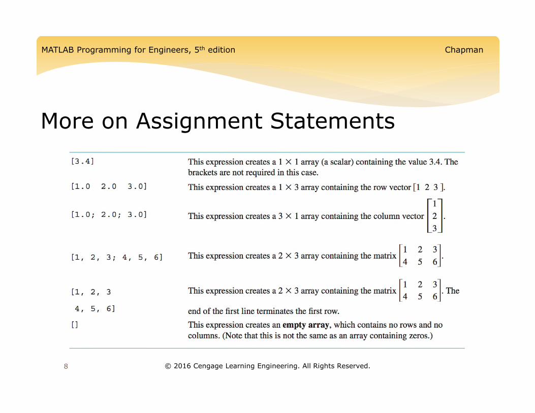
More on Assignment Statements
MATLAB Programming for Engineers, 5th edition Chapman
© 2016 Cengage Learning Engineering. All Rights Reserved. 9
Initializing with Shortcut Expressions
∗ The colon operator specifies a whole series of values by specifying the first value in the series, the stepping increment, and the last value in the series
∗ first:incr:last
∗ The transpose operator (denoted by an apostrophe) swaps the row and columns of any array to which it is applied
MATLAB Programming for Engineers, 5th edition Chapman
© 2016 Cengage Learning Engineering. All Rights Reserved. 10
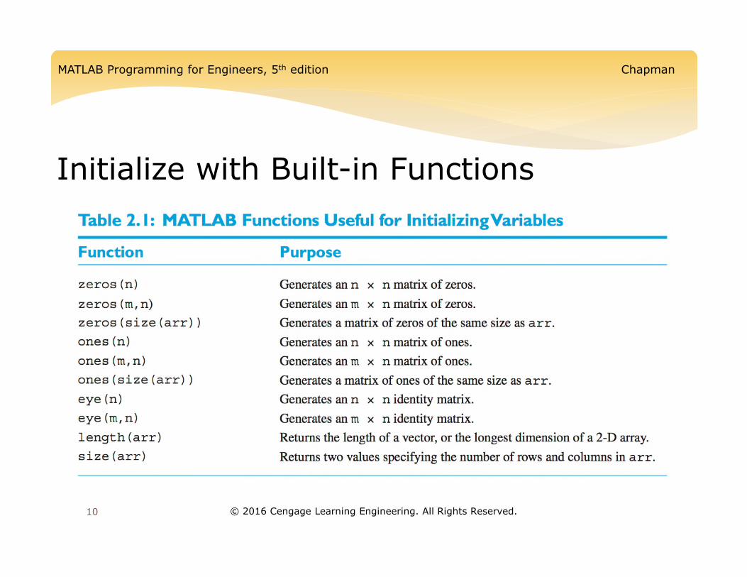
Initialize with Built-in Functions
MATLAB Programming for Engineers, 5th edition Chapman
© 2016 Cengage Learning Engineering. All Rights Reserved. 11
2.3 Multidimensional Arrays
∗ MATLAB allows us to create arrays with as many dimensions as needed for a particular problem.
∗ You access an element in an array using its indices:∗ a(1, 5) a(:, :, 1) a(5)
∗ MATLAB always allocates array elements in column major order, i.e., allocating the first column in memory, then the second, then the third, etc.
MATLAB Programming for Engineers, 5th edition Chapman
© 2016 Cengage Learning Engineering. All Rights Reserved. 12
2.4 Subarrays
∗ It is possible to select and use subsets of MATLAB arrays as though they were separate arrays
∗ To select a portion of an array, just include a list of all of the elements to be selected in the parentheses after the array name
∗ When used in an array subscript, the special function endreturns the highest value taken on by that subscript
arr3 = [1 2 3 4 5 6 7 8];arr3(5:end) = [5 6 7 8]
MATLAB Programming for Engineers, 5th edition Chapman
© 2016 Cengage Learning Engineering. All Rights Reserved. 13
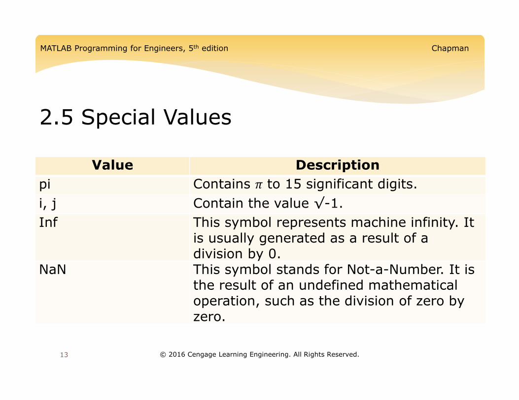
2.5 Special Values
Value Description
pi Contains π to 15 significant digits.
i, j Contain the value √-1.
Inf This symbol represents machine infinity. It is usually generated as a result of a division by 0.
NaN This symbol stands for Not-a-Number. It is the result of an undefined mathematical operation, such as the division of zero by zero.
MATLAB Programming for Engineers, 5th edition Chapman
© 2016 Cengage Learning Engineering. All Rights Reserved. 14
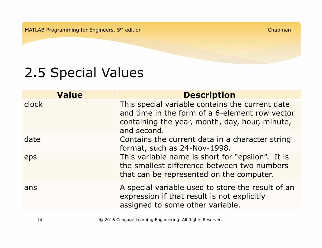
2.5 Special Values
Value Descriptionclock This special variable contains the current date
and time in the form of a 6-element row vector containing the year, month, day, hour, minute, and second.
date Contains the current data in a character string format, such as 24-Nov-1998.
eps This variable name is short for “epsilon”. It is the smallest difference between two numbers that can be represented on the computer.
ans A special variable used to store the result of an expression if that result is not explicitly assigned to some other variable.
MATLAB Programming for Engineers, 5th edition Chapman
© 2016 Cengage Learning Engineering. All Rights Reserved. 15
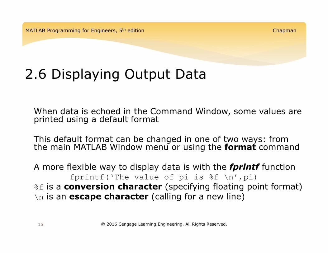
2.6 Displaying Output Data
∗ When data is echoed in the Command Window, some values are printed using a default format
∗ This default format can be changed in one of two ways: from the main MATLAB Window menu or using the format command
∗ A more flexible way to display data is with the fprintf functionfprintf(‘The value of pi is %f \n’,pi)
∗ %f is a conversion character (specifying floating point format)∗ \n is an escape character (calling for a new line)
MATLAB Programming for Engineers, 5th edition Chapman
© 2016 Cengage Learning Engineering. All Rights Reserved. 16
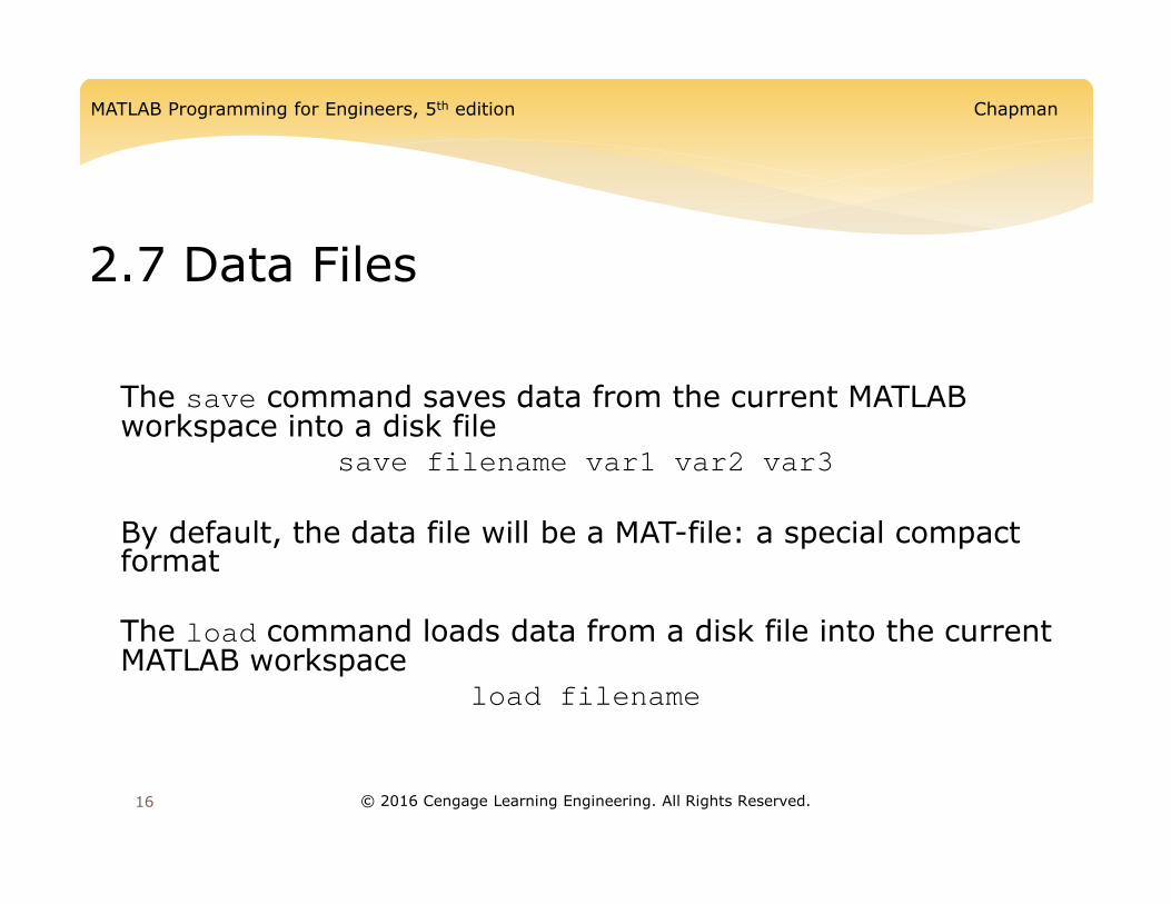
2.7 Data Files
∗ The save command saves data from the current MATLAB workspace into a disk file
save filename var1 var2 var3
∗ By default, the data file will be a MAT-file: a special compact format
∗ The load command loads data from a disk file into the current MATLAB workspace
load filename
MATLAB Programming for Engineers, 5th edition Chapman
© 2016 Cengage Learning Engineering. All Rights Reserved. 17
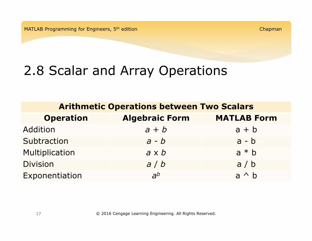
2.8 Scalar and Array Operations
Arithmetic Operations between Two Scalars
Operation Algebraic Form MATLAB Form
Addition a + b a + b
Subtraction a - b a - b
Multiplication a x b a * b
Division a / b a / b
Exponentiation ab a ^ b
MATLAB Programming for Engineers, 5th edition Chapman
© 2016 Cengage Learning Engineering. All Rights Reserved. 18
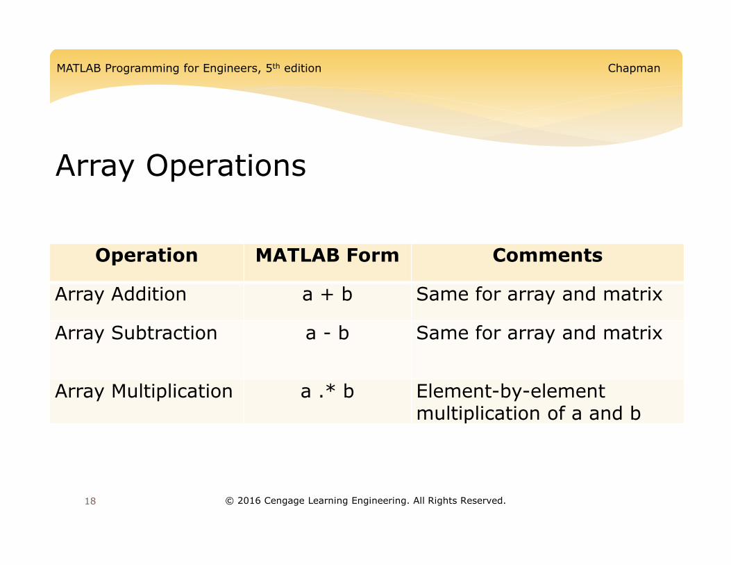
Array Operations
Operation MATLAB Form Comments
Array Addition a + b Same for array and matrix
Array Subtraction a - b Same for array and matrix
Array Multiplication a .* b Element-by-element multiplication of a and b
MATLAB Programming for Engineers, 5th edition Chapman
© 2016 Cengage Learning Engineering. All Rights Reserved. 19
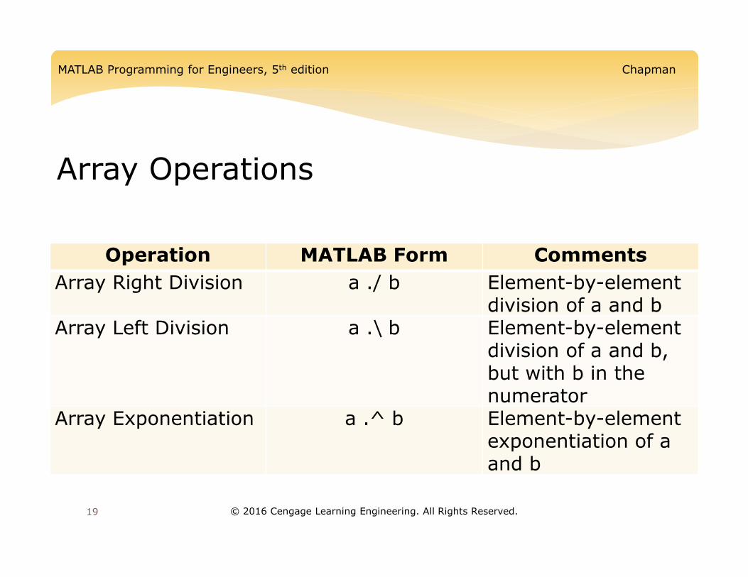
Array Operations
Operation MATLAB Form Comments
Array Right Division a ./ b Element-by-element division of a and b
Array Left Division a .\ b Element-by-element division of a and b, but with b in the numerator
Array Exponentiation a .^ b Element-by-element exponentiation of aand b
MATLAB Programming for Engineers, 5th edition Chapman
© 2016 Cengage Learning Engineering. All Rights Reserved. 20
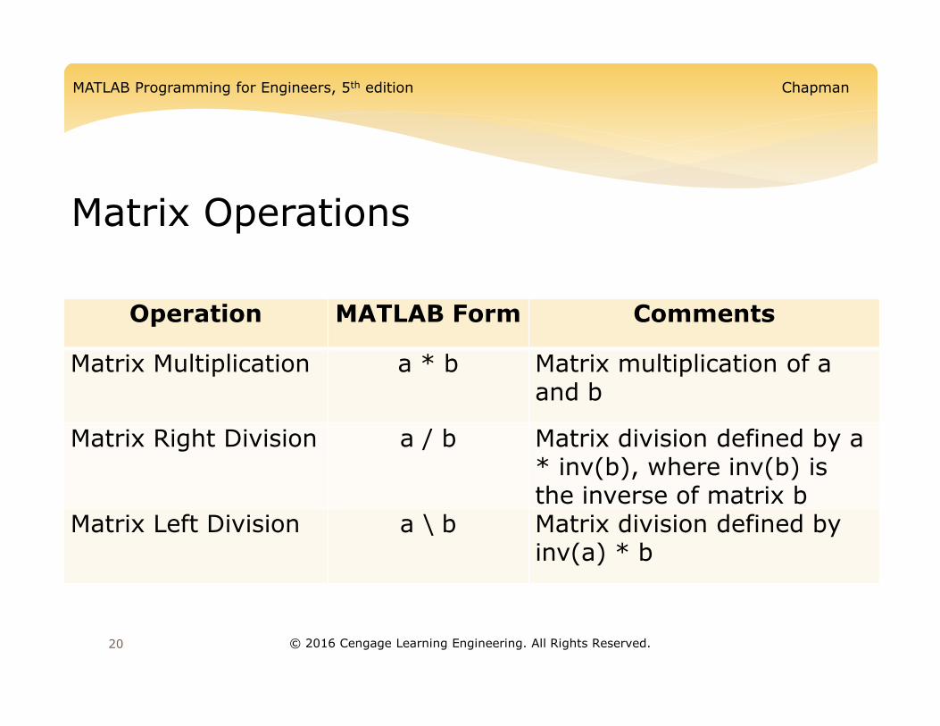
Matrix Operations
Operation MATLAB Form Comments
Matrix Multiplication a * b Matrix multiplication of aand b
Matrix Right Division a / b Matrix division defined by a * inv(b), where inv(b) is the inverse of matrix b
Matrix Left Division a \ b Matrix division defined by inv(a) * b
MATLAB Programming for Engineers, 5th edition Chapman
© 2016 Cengage Learning Engineering. All Rights Reserved. 21
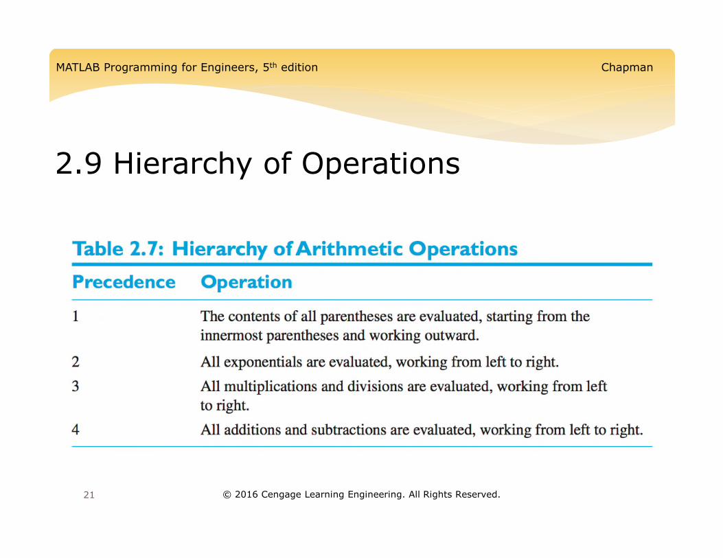
2.9 Hierarchy of Operations

MATLAB Programming for Engineers, 5th edition Chapman
© 2016 Cengage Learning Engineering. All Rights Reserved. 22
2.10 Built-in MATLAB Functions
∗ One of MATLAB’s greatest strengths is that it comes with an incredible variety of built-in functions ready for use
∗ Unlike mathematical functions, MATLAB functions can return more than one result to the calling program. For example,
[maxval, index] = max([1 –5 6 –3])
∗ Some functions, like sin and cos, can take an array of input values and calculate an array of output values on an element-by-element basis (refer to Table 2.8 in the text for a long list of common functions)
MATLAB Programming for Engineers, 5th edition Chapman
© 2016 Cengage Learning Engineering. All Rights Reserved. 23
2.11 Introduction to Plotting
∗ To plot a data set, just create two vectors containing the x and y values to be plotted, and use the plot function
x = 0:1:10;y = x.ˆ2 – 10.*x + 15;
plot(x,y)
∗ MATLAB allows a programmer to select the color of a line to be plotted, the style of the line to be plotted, and the type of marker to be used for data points on the line
plot(x,y,‘r--’)
MATLAB Programming for Engineers, 5th edition Chapman
© 2016 Cengage Learning Engineering. All Rights Reserved. 24
2.13 Debugging MATLAB Programs
∗ There are three types of errors found in MATLAB programs:
1. Syntax error – errors in the statement like spelling and punctuation
2. Run-time error – illegal mathematical operation attempted
3. Logical error – runs but produces wrong answer
MATLAB includes a special debugging tool called a symbolic debugger, which allows you to walk through the execution of your program one statement at a time and to examine the values of any variables at each step along the way
MATLAB Programming for Engineers, 5th edition Chapman
© 2016 Cengage Learning Engineering. All Rights Reserved. 25
2.14 Summary
∗ Introduced two data types (double and char), assignment statements, input/output statements, and data files
∗ Listed arithmetic operations for scalars, array operations, and matrix operations
∗ Quick look at built-in functions, plotting, and debugging