2 | LIMITS OF LEARNING

Dependencies: None.

Machine learning is a very general and useful framework,but it is not “magic” and will not always work. In order to betterunderstand when it will and when it will not work, it is useful toformalize the learning problem more. This will also help us developdebugging strategies for learning algorithms.

2.1 Data Generating Distributions

Our underlying assumption for the majority of this book is thatlearning problems are characterized by some unknown probabilitydistribution D over input/output pairs (x, y) ∈ X×Y . Suppose thatsomeone told you what D was. In particular, they gave you a Pythonfunction computeD that took two inputs, x and y, and returned theprobability of that x, y pair under D. If you had access to such a func-tion, classification becomes simple. We can define the Bayes optimalclassifier as the classifier that, for any test input x, simply returns they that maximizes computeD(x, y), or, more formally:

f (BO)(x) = arg maxy∈YD(x, y) (2.1)

This classifier is optimal in one specific sense: of all possible classifiers,it achieves the smallest zero/one error.

Theorem 1 (Bayes Optimal Classifier). The Bayes Optimal Classifierf (BO) achieves minimal zero/one error of any deterministic classifier.

This theorem assumes that you are comparing against deterministicclassifiers. You can actually prove a stronger result that f (BO) is opti-mal for randomized classifiers as well, but the proof is a bit messier.However, the intuition is the same: for a given x, f (BO) chooses thelabel with highest probability, thus minimizing the probability that itmakes an error.

Proof of Theorem 1. Consider some other classifier g that claims tobe better than f (BO). Then, there must be some x on which g(x) 6=

Learning Objectives:• Define “inductive bias” and recog-

nize the role of inductive bias inlearning.

• Illustrate how regularization tradesoff between underfitting and overfit-ting.

• Evaluate whether a use of test datais “cheating” or not.

Our lives sometimes depend on computers performing as pre-dicted. – Philip Emeagwali

20 a course in machine learning

f (BO)(x). Fix such an x. Now, the probability that f (BO) makes an erroron this particular x is 1− D(x, f (BO)(x)) and the probability that gmakes an error on this x is 1− D(x, g(x)). But f (BO) was chosen insuch a way to maximize D(x, f (BO)(x)), so this must be greater thanD(x, g(x)). Thus, the probability that f (BO) errs on this particular x issmaller than the probability that g errs on it. This applies to any x forwhich f (BO)(x) 6= g(x) and therefore f (BO) achieves smaller zero/oneerror than any g.

The Bayes error rate (or Bayes optimal error rate) is the errorrate of the Bayes optimal classifier. It is the best error rate you canever hope to achieve on this classification problem (under zero/oneloss). The take-home message is that if someone gave you access tothe data distribution, forming an optimal classifier would be trivial.Unfortunately, no one gave you this distribution, so we need to figureout ways of learning the mapping from x to y given only access to atraining set sampled from D, rather than D itself.

2.2 Inductive Bias: What We Know Before the Data Arrives

class A

clas

sB

Figure 2.1: Training data for a binaryclassification problem.

Figure 2.2: Test data for the sameclassification problem.

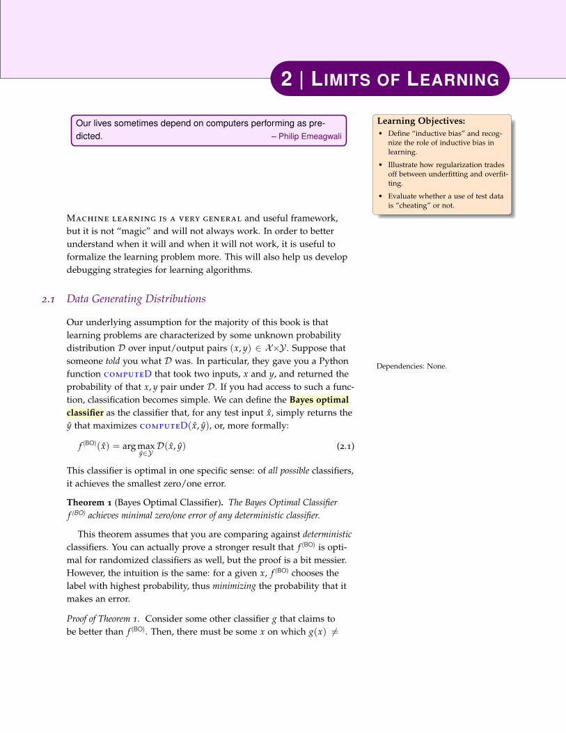
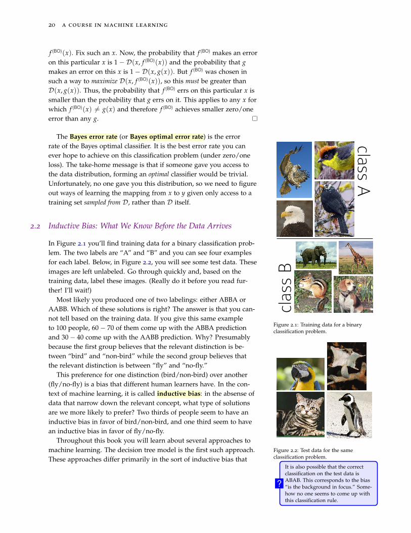
In Figure 2.1 you’ll find training data for a binary classification prob-lem. The two labels are “A” and “B” and you can see four examplesfor each label. Below, in Figure 2.2, you will see some test data. Theseimages are left unlabeled. Go through quickly and, based on thetraining data, label these images. (Really do it before you read fur-ther! I’ll wait!)

Most likely you produced one of two labelings: either ABBA orAABB. Which of these solutions is right? The answer is that you can-not tell based on the training data. If you give this same exampleto 100 people, 60− 70 of them come up with the ABBA predictionand 30− 40 come up with the AABB prediction. Why? Presumablybecause the first group believes that the relevant distinction is be-tween “bird” and “non-bird” while the second group believes thatthe relevant distinction is between “fly” and “no-fly.”

This preference for one distinction (bird/non-bird) over another(fly/no-fly) is a bias that different human learners have. In the con-text of machine learning, it is called inductive bias: in the absense ofdata that narrow down the relevant concept, what type of solutionsare we more likely to prefer? Two thirds of people seem to have aninductive bias in favor of bird/non-bird, and one third seem to havean inductive bias in favor of fly/no-fly.

It is also possible that the correctclassification on the test data isABAB. This corresponds to the bias“is the background in focus.” Some-how no one seems to come up withthis classification rule.

?

Throughout this book you will learn about several approaches tomachine learning. The decision tree model is the first such approach.These approaches differ primarily in the sort of inductive bias that

limits of learning 21

they exhibit.Consider a variant of the decision tree learning algorithm. In this

variant, we will not allow the trees to grow beyond some pre-definedmaximum depth, d. That is, once we have queried on d-many fea-tures, we cannot query on any more and must just make the bestguess we can at that point. This variant is called a shallow decisiontree.

The key question is: What is the inductive bias of shallow decisiontrees? Roughly, their bias is that decisions can be made by only look-ing at a small number of features. For instance, a shallow decisiontree would be very good at learning a function like “students onlylike AI courses.” It would be very bad at learning a function like “ifthis student has liked an odd number of their past courses, they willlike the next one; otherwise they will not.” This latter is the parityfunction, which requires you to inspect every feature to make a pre-diction. The inductive bias of a decision tree is that the sorts of thingswe want to learn to predict are more like the first example and lesslike the second example.

2.3 Not Everything is Learnable

Although machine learning works well—perhaps astonishinglywell—in many cases, it is important to keep in mind that it is notmagical. There are many reasons why a machine learning algorithmmight fail on some learning task.

There could be noise in the training data. Noise can occur bothat the feature level and at the label level. Some features might corre-spond to measurements taken by sensors. For instance, a robot mightuse a laser range finder to compute its distance to a wall. However,this sensor might fail and return an incorrect value. In a sentimentclassification problem, someone might have a typo in their review ofa course. These would lead to noise at the feature level. There mightalso be noise at the label level. A student might write a scathinglynegative review of a course, but then accidentally click the wrongbutton for the course rating.

The features available for learning might simply be insufficient.For example, in a medical context, you might wish to diagnosewhether a patient has cancer or not. You may be able to collect alarge amount of data about this patient, such as gene expressions,X-rays, family histories, etc. But, even knowing all of this informationexactly, it might still be impossible to judge for sure whether this pa-tient has cancer or not. As a more contrived example, you might tryto classify course reviews as positive or negative. But you may haveerred when downloading the data and only gotten the first five char-

22 a course in machine learning

acters of each review. If you had the rest of the features you mightbe able to do well. But with this limited feature set, there’s not muchyou can do.

Some examples may not have a single correct answer. You mightbe building a system for “safe web search,” which removes offen-sive web pages from search results. To build this system, you wouldcollect a set of web pages and ask people to classify them as “offen-sive” or not. However, what one person considers offensive might becompletely reasonable for another person. It is common to considerthis as a form of label noise. Nevertheless, since you, as the designerof the learning system, have some control over this problem, it issometimes helpful to isolate it as a source of difficulty.

Finally, learning might fail because the inductive bias of the learn-ing algorithm is too far away from the concept that is being learned.In the bird/non-bird data, you might think that if you had gottena few more training examples, you might have been able to tellwhether this was intended to be a bird/non-bird classification or afly/no-fly classification. However, no one I’ve talked to has ever comeup with the “background is in focus” classification. Even with manymore training points, this is such an unusual distinction that it maybe hard for anyone to figure out it. In this case, the inductive bias ofthe learner is simply too misaligned with the target classification tolearn.

Note that the inductive bias source of error is fundamentally dif-ferent than the other three sources of error. In the inductive bias case,it is the particular learning algorithm that you are using that cannotcope with the data. Maybe if you switched to a different learningalgorithm, you would be able to learn well. For instance, Neptuniansmight have evolved to care greatly about whether backgrounds arein focus, and for them this would be an easy classification to learn.For the other three sources of error, it is not an issue to do with theparticular learning algorithm. The error is a fundamental part of thelearning problem.

2.4 Underfitting and Overfitting

As with many problems, it is useful to think about the extreme casesof learning algorithms. In particular, the extreme cases of decisiontrees. In one extreme, the tree is “empty” and we do not ask anyquestions at all. We simply immediately make a prediction. In theother extreme, the tree is “full.” That is, every possible questionis asked along every branch. In the full tree, there may be leaveswith no associated training data. For these we must simply choosearbitrarily whether to say “yes” or “no.”

limits of learning 23

Consider the course recommendation data from Table 1. Sup-pose we were to build an “empty” decision tree on this data. Such adecision tree will make the same prediction regardless of its input,because it is not allowed to ask any questions about its input. Sincethere are more “likes” than “hates” in the training data (12 versus8), our empty decision tree will simply always predict “likes.” Thetraining error, ε, is 8/20 = 40%.

On the other hand, we could build a “full” decision tree. Sinceeach row in this data is unique, we can guarantee that any leaf in afull decision tree will have either 0 or 1 examples assigned to it (20of the leaves will have one example; the rest will have none). For theleaves corresponding to training points, the full decision tree willalways make the correct prediction. Given this, the training error, ε, is0/20 = 0%.

Of course our goal is not to build a model that gets 0% error onthe training data. This would be easy! Our goal is a model that willdo well on future, unseen data. How well might we expect these twomodels to do on future data? The “empty” tree is likely to do notmuch better and not much worse on future data. We might expectthat it would continue to get around 40% error.

Life is more complicated for the “full” decision tree. Certainlyif it is given a test example that is identical to one of the trainingexamples, it will do the right thing (assuming no noise). But foreverything else, it will only get about 50% error. This means thateven if every other test point happens to be identical to one of thetraining points, it would only get about 25% error. In practice, this isprobably optimistic, and maybe only one in every 10 examples wouldmatch a training example, yielding a 35% error. Convince yourself (either by proof

or by simulation) that even in thecase of imbalanced data – for in-stance data that is on average 80%positive and 20% negative – a pre-dictor that guesses randomly (50/50

positive/negative) will get about50% error.

?

So, in one case (empty tree) we’ve achieved about 40% error andin the other case (full tree) we’ve achieved 35% error. This is notvery promising! One would hope to do better! In fact, you mightnotice that if you simply queried on a single feature for this data, youwould be able to get very low training error, but wouldn’t be forcedto “guess” randomly.

Which feature is it, and what is it’straining error??

This example illustrates the key concepts of underfitting andoverfitting. Underfitting is when you had the opportunity to learnsomething but didn’t. A student who hasn’t studied much for an up-coming exam will be underfit to the exam, and consequently will notdo well. This is also what the empty tree does. Overfitting is whenyou pay too much attention to idiosyncracies of the training data,and aren’t able to generalize well. Often this means that your modelis fitting noise, rather than whatever it is supposed to fit. A studentwho memorizes answers to past exam questions without understand-ing them has overfit the training data. Like the full tree, this student

24 a course in machine learning

Consider some random event, like spins of a roulette wheel, cars driving through an intersection, theoutcome of an election, or pasta being appropriately al dente. We often want to make a conclusionabout the entire population (the pot of pasta) based on a much smaller sample (biting a couple piecesof pasta). The law of large numbers tells us that under mild conditions this is an okay thing to do.

Formally, suppose that v1, v2, . . . , vN are random variables (e.g., vn measures if the nth spaghetti isal dente). Assume that these random variables are independent (i.e., v2 and v3 are uncorrelated—they weren’t both taken from the same place in the pot) and identically distributed (they were alldrawn from the same population—pot—that we wish to measure). We can compute the sample av-erage v = 1

N ∑Nn=1 vn and under the strong law of large numbers, you can prove that v → E[v] as

N → ∞. Namely, the empirical sample average approaches the population average as the number ofsamples goes do infinity.

(Technical note: the notion of convergence here is almost sure convergence. In particular, the formal result isthat Pr

(limN→∞

1N ∑n vn = E[v]

)= 1. Or, in words, with probability one the sample average reaches the

population average.)

MATH REVIEW | LAW OF LARGE NUMBERS

Figure 2.3:

also will not do well on the exam. A model that is neither overfit norunderfit is the one that is expected to do best in the future.

2.5 Separation of Training and Test Data

Suppose that, after graduating, you get a job working for a companythat provides personalized recommendations for pottery. You go inand implement new algorithms based on what you learned in yourmachine learning class (you have learned the power of generaliza-tion!). All you need to do now is convince your boss that you havedone a good job and deserve a raise!

How can you convince your boss that your fancy learning algo-rithms are really working?

Based on what we’ve talked about already with underfitting andoverfitting, it is not enough to just tell your boss what your trainingerror is. Noise notwithstanding, it is easy to get a training error ofzero using a simple database query (or grep, if you prefer). Your bosswill not fall for that.

The easiest approach is to set aside some of your available data as“test data” and use this to evaluate the performance of your learningalgorithm. For instance, the pottery recommendation service that youwork for might have collected 1000 examples of pottery ratings. Youwill select 800 of these as training data and set aside the final 200

limits of learning 25

as test data. You will run your learning algorithms only on the 800training points. Only once you’re done will you apply your learnedmodel to the 200 test points, and report your test error on those 200points to your boss.

The hope in this process is that however well you do on the 200test points will be indicative of how well you are likely to do in thefuture. This is analogous to estimating support for a presidentialcandidate by asking a small (random!) sample of people for theiropinions. Statistics (specifically, concentration bounds of which the“Central limit theorem” is a famous example) tells us that if the sam-ple is large enough, it will be a good representative. The 80/20 splitis not magic: it’s simply fairly well established. Occasionally peopleuse a 90/10 split instead, especially if they have a lot of data. If you have more data at your dis-

posal, why might a 90/10 split bepreferable to an 80/20 split?

?The cardinal rule of machine learning is: never touch your testdata. Ever. If that’s not clear enough:

Never ever touch your test data!If there is only one thing you learn from this book, let it be that.

Do not look at your test data. Even once. Even a tiny peek. Onceyou do that, it is not test data any more. Yes, perhaps your algorithmhasn’t seen it. But you have. And you are likely a better learner thanyour learning algorithm. Consciously or otherwise, you might makedecisions based on whatever you might have seen. Once you look atthe test data, your model’s performance on it is no longer indicativeof it’s performance on future unseen data. This is simply becausefuture data is unseen, but your “test” data no longer is.

2.6 Models, Parameters and Hyperparameters

The general approach to machine learning, which captures many ex-isting learning algorithms, is the modeling approach. The idea is thatwe come up with some formal model of our data. For instance, wemight model the classification decision of a student/course pair as adecision tree. The choice of using a tree to represent this model is ourchoice. We also could have used an arithmetic circuit or a polynomialor some other function. The model tells us what sort of things we canlearn, and also tells us what our inductive bias is.

For most models, there will be associated parameters. These arethe things that we use the data to decide on. Parameters in a decisiontree include: the specific questions we asked, the order in which weasked them, and the classification decisions at the leaves. The job ofour decision tree learning algorithm DecisionTreeTrain is to takedata and figure out a good set of parameters.

26 a course in machine learning

Many learning algorithms will have additional knobs that you canadjust. In most cases, these knobs amount to tuning the inductivebias of the algorithm. In the case of the decision tree, an obviousknob that one can tune is the maximum depth of the decision tree.That is, we could modify the DecisionTreeTrain function so thatit stops recursing once it reaches some pre-defined maximum depth.By playing with this depth knob, we can adjust between underfitting(the empty tree, depth= 0) and overfitting (the full tree, depth= ∞). Go back to the DecisionTree-

Train algorithm and modify it sothat it takes a maximum depth pa-rameter. This should require addingtwo lines of code and modifyingthree others.

?Such a knob is called a hyperparameter. It is so called because it

is a parameter that controls other parameters of the model. The exactdefinition of hyperparameter is hard to pin down: it’s one of thosethings that are easier to identify than define. However, one of thekey identifiers for hyperparameters (and the main reason that theycause consternation) is that they cannot be naively adjusted using thetraining data.

In DecisionTreeTrain, as in most machine learning, the learn-ing algorithm is essentially trying to adjust the parameters of themodel so as to minimize training error. This suggests an idea forchoosing hyperparameters: choose them so that they minimize train-ing error.

What is wrong with this suggestion? Suppose that you were totreat “maximum depth” as a hyperparameter and tried to tune it onyour training data. To do this, maybe you simply build a collectionof decision trees, tree0, tree1, tree2, . . . , tree100, where treed is a treeof maximum depth d. We then computed the training error of eachof these trees and chose the “ideal” maximum depth as that whichminimizes training error? Which one would it pick?

The answer is that it would pick d = 100. Or, in general, it wouldpick d as large as possible. Why? Because choosing a bigger d willnever hurt on the training data. By making d larger, you are simplyencouraging overfitting. But by evaluating on the training data, over-fitting actually looks like a good idea!

An alternative idea would be to tune the maximum depth on testdata. This is promising because test data peformance is what wereally want to optimize, so tuning this knob on the test data seemslike a good idea. That is, it won’t accidentally reward overfitting. Ofcourse, it breaks our cardinal rule about test data: that you shouldnever touch your test data. So that idea is immediately off the table.

However, our “test data” wasn’t magic. We simply took our 1000examples, called 800 of them “training” data and called the other 200“test” data. So instead, let’s do the following. Let’s take our original1000 data points, and select 700 of them as training data. From theremainder, take 100 as development data1 and the remaining 200 1 Some people call this “validation

data” or “held-out data.”as test data. The job of the development data is to allow us to tune

limits of learning 27

hyperparameters. The general approach is as follows:

1. Split your data into 70% training data, 10% development data and20% test data.

2. For each possible setting of your hyperparameters:

(a) Train a model using that setting of hyperparameters on thetraining data.

(b) Compute this model’s error rate on the development data.

3. From the above collection of models, choose the one that achievedthe lowest error rate on development data.

4. Evaluate that model on the test data to estimate future test perfor-mance.

In step 3, you could either choosethe model (trained on the 70% train-ing data) that did the best on thedevelopment data. Or you couldchoose the hyperparameter settingsthat did best and retrain the modelon the 80% union of training anddevelopment data. Is either of theseoptions obviously better or worse?

?2.7 Real World Applications of Machine Learning

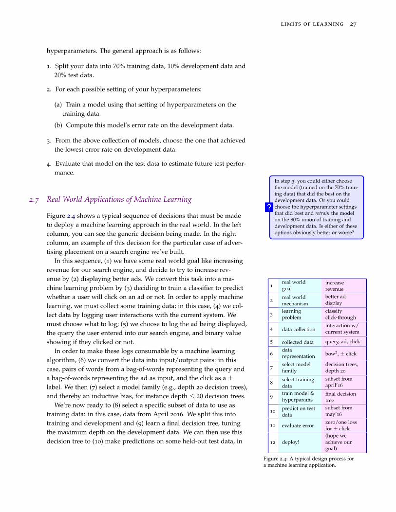
Figure 2.4 shows a typical sequence of decisions that must be madeto deploy a machine learning approach in the real world. In the leftcolumn, you can see the generic decision being made. In the rightcolumn, an example of this decision for the particular case of adver-tising placement on a search engine we’ve built.

In this sequence, (1) we have some real world goal like increasingrevenue for our search engine, and decide to try to increase rev-enue by (2) displaying better ads. We convert this task into a ma-chine learning problem by (3) deciding to train a classifier to predictwhether a user will click on an ad or not. In order to apply machinelearning, we must collect some training data; in this case, (4) we col-lect data by logging user interactions with the current system. Wemust choose what to log; (5) we choose to log the ad being displayed,the query the user entered into our search engine, and binary valueshowing if they clicked or not.

1

real worldgoal

increaserevenue

2real worldmechanism

better addisplay

3learningproblem

classifyclick-through

4 data collectioninteraction w/current system

5 collected data query, ad, click

6

datarepresentation bow2, ± click

7select modelfamily

decision trees,depth 20

8select trainingdata

subset fromapril’16

9train model &hyperparams

final decisiontree

10predict on testdata

subset frommay’16

11 evaluate errorzero/one lossfor ± click

12 deploy!(hope weachieve ourgoal)

Figure 2.4: A typical design process fora machine learning application.

In order to make these logs consumable by a machine learningalgorithm, (6) we convert the data into input/output pairs: in thiscase, pairs of words from a bag-of-words representing the query anda bag-of-words representing the ad as input, and the click as a ±label. We then (7) select a model family (e.g., depth 20 decision trees),and thereby an inductive bias, for instance depth ≤ 20 decision trees.

We’re now ready to (8) select a specific subset of data to use astraining data: in this case, data from April 2016. We split this intotraining and development and (9) learn a final decision tree, tuningthe maximum depth on the development data. We can then use thisdecision tree to (10) make predictions on some held-out test data, in

28 a course in machine learning

this case from the following month. We can (11) measure the overallquality of our predictor as zero/one loss (clasification error) on thistest data and finally (12) deploy our system.

The important thing about this sequence of steps is that in anyone, things can go wrong. That is, between any two rows of this table,we are necessarily accumulating some additional error against ouroriginal real world goal of increasing revenue. For example, in step 5,we decided on a representation that left out many possible variableswe could have logged, like time of day or season of year. By leavingout those variables, we set an explicit upper bound on how well ourlearned system can do.

It is often an effective strategy to run an oracle experiment. In anoracle experiment, we assume that everything below some line can besolved perfectly, and measure how much impact that will have on ahigher line. As an extreme example, before embarking on a machinelearning approach to the ad display problem, we should measuresomething like: if our classifier were perfect, how much more moneywould we make? If the number is not very high, perhaps there issome better for our time.

Finally, although this sequence is denoted linearly, the entire pro-cess is highly interactive in practice. A large part of “debugging”machine learning (covered more extensively in Chapter 5 involvestrying to figure out where in this sequence the biggest losses are andfixing that step. In general, it is often useful to build the stupidest thingthat could possibly work, then look at how well it’s doing, and decide ifand where to fix it.

2.8 Further Reading

TODO further reading