Embed Size (px)
Citation preview

2. Introduction to the Relational Model and SQL 2-1
Part 2: Introduction to theRelational Model and SQL
References:• Elmasri/Navathe: Fundamentals of Database Systems, 3rd Edition, 1999.
Section 7.1, “Relational Model Concepts”Section 8.2, “Basic Queries in SQL”
• Kemper/Eickler: Datenbanksysteme (in German), 3rd Edition, 1999.Section 3.1, “Definition des relationalen Modells” (“Definition of the Relational Model”)Section 4.6, “Einfache SQL-Anfragen” (“Simple SQL Queries”)
• Lipeck: Skript zur Vorlesung Datenbanksysteme (in German), Univ. Hannover, 1996.
• Sunderraman: Oracle Programming, A Primer. Addison-Wesley, 1999.
• Oracle8i SQL Reference, Rel. 2 (8.1.6), Oracle Corp., Dec. 1999, Part No. A76989-01.
• SQL*Plus: Quick Reference, Rel. 8.1.6, Oracle Corp., Oct. 1999, Part No. 75665-01.
• SQL*Plus: User’s Guide and Reference, Rel. 8.1.6, Oct. 1999, Part No. A75664-01.
• Codd: A relational model of data for large shared data banks. Communications of theACM, 13(6), 377–387, 1970.
• Boyce/Chamberlin: SEQUEL: A structured English query language. In ACM SIGMODConf. on the Management of Data, 1974.
• Astrahan et al: System R: A relational approach to database management. ACM Tran-sactions on Database Systems 1(2), 97–137, 1976.
Stefan Brass: Database Systems Universitat Halle, 2003

2. Introduction to the Relational Model and SQL 2-2
Objectives
After completing this chapter, you should be able to:
• explain the basic notions of the relational model:
table/relation, row/tuple, column/attribute,
column value/attribute value.
• explain the meaning of keys and foreign keys.
• write simple SQL queries (queries to one table).
• use Oracle SQL*Plus for evaluating queries.
Stefan Brass: Database Systems Universitat Halle, 2003

2. Introduction to the Relational Model and SQL 2-3
Overview
1. The Relational Model, Example Database
'
&
$
%2. Using SQL*Plus: First Demonstration
3. Simple SQL Queries
4. Historical Remarks
Stefan Brass: Database Systems Universitat Halle, 2003

2. Introduction to the Relational Model and SQL 2-4
The Relational Model (1)
• The relational model structures data in table form,
i.e. a relational DB is a set of named tables.
• A relational database schema defines:
� Names of tables in the database.
� The columns of each table, i.e. the column na-
mes and the data types of the column entries.The columns have a sequence (first column, second column, etc.).Each column can store only data of a particular type, e.g. strings,numbers of a certain length and precision, date values, etc.
� Integrity constraints.Integrity constraints are conditions that the data must satisfy.
Stefan Brass: Database Systems Universitat Halle, 2003

2. Introduction to the Relational Model and SQL 2-5
The Relational Model (2)
• For instance, Oracle comes with an example data-
base that consists of three tables:
� EMP: Information about employees.
� DEPT: Information about departments.
� SALGRADE: Information about salary ranges
for different levels/grades.
This table is not used in the following example queries.
• Depending on the version of the example database,
there might be further tables.
Stefan Brass: Database Systems Universitat Halle, 2003

2. Introduction to the Relational Model and SQL 2-6
The Relational Model (3)
• The Table DEPT has the following columns:
� DEPTNO: Department Number,
� DNAME: Department Name,
� LOC: Location.
DEPT
DEPTNO DNAME LOC
10 ACCOUNTING NEW YORK
20 RESEARCH DALLAS
30 SALES CHICAGO
40 OPERATIONS BOSTON
Stefan Brass: Database Systems Universitat Halle, 2003
2. Introduction to the Relational Model and SQL 2-7
The Relational Model (4)
The columns have the following data types:
• DEPTNO has the data type NUMERIC(2),
i.e. can be a two-digit integer from -99 to +99.
Obviously, one does not want negative department numbers.They can be excluded by means of constraints.
• DNAME has the type VARCHAR(14), i.e. is a character
string of variable length that consists of at most
14 characters.
• LOC has the type VARCHAR(13).
The data dictionary (system catalog) lists types NUMBER(2), VARCHAR2(14), andVARCHAR2(13). These are Oracle-specific names for the types listed above.
Stefan Brass: Database Systems Universitat Halle, 2003

2. Introduction to the Relational Model and SQL 2-8
The Relational Model (5)
• A relational database state (instance of a given
schema) defines for each table a set of rows.
• The example table “DEPT” has currently four rows.
• The relational model does not define any particular
order of the rows (e.g. which is first, second, etc.).
But rows can be sorted for output.
• Each row specifies values for the columns of the
table.
E.g. one row above has the value 10 for the column DEPTNO, the value’ACCOUNTING’ for DNAME, and ’NEW YORK’ for LOC.
Stefan Brass: Database Systems Universitat Halle, 2003

2. Introduction to the Relational Model and SQL 2-9
Summary (1)
R
Table NamePPPPPPPPPq
A1 · · · An
ColumnPPPPPPPPq
Column��������)
a1,1
...am,1
· · ·...
· · ·
a1,n
...am,n
Row -
Row -
�������)
TableEntry
(ColumnValue)
Stefan Brass: Database Systems Universitat Halle, 2003

2. Introduction to the Relational Model and SQL 2-10
Summary (2)
• A more theoretically oriented person would use the
following synonyms:
� Relation instead of table.
A table is formally a subset of the cartesian product of the domainsof the columns, and that is called a relation in mathematics. Car-tesian coordinates are (X, Y )-pairs of real numbers, i.e. elementsof IR × IR. The relation < can also be understood as a subset ofIR × IR (e.g. (1,2) is contained in the relation, and (2,1) is notcontained in the relation). However, database relations are alwaysfinite and they may have more than two columns.
� Tuple instead of row.
� Attribute instead of column.
Stefan Brass: Database Systems Universitat Halle, 2003

2. Introduction to the Relational Model and SQL 2-11
Summary (3)
• Old-style practical people might say
� record instead of row,
A table row (tuple) is basically the same as a record in Pascal ora structure in C: It has several named components. However, thestorage structure of a tuple in external memory (on the disk) isnot necessarily the same as that of a record in main memory.
� field instead of column,
� field value instead of table entry,
� file instead of table.
That should be avoided since it is confusing: Modern DBMS mightstore many tables in the same operating system file, and they mayalso split the same table over different files.
Stefan Brass: Database Systems Universitat Halle, 2003

2. Introduction to the Relational Model and SQL 2-12
Keys (1)
• The column DEPTNO is declared as a “key” of the
table DEPT.
• That means that a value for DEPTNO always uniquely
identifies a single row in the table.
• For instance, the table already contains a row with
DEPTNO = 10.
• If one tries to add another row with the same va-
lue 10 for DEPTNO, one gets an error message.
Stefan Brass: Database Systems Universitat Halle, 2003

2. Introduction to the Relational Model and SQL 2-13
Keys (2)
• Keys are an example of constraints: Conditions that
the table contents (DB state) must satisfy in addi-
tion to the basic structure given by the columns.
• Constraints are declared as part of the DB schema.
• More than one key can be declared for a table.
E.g., one could discuss whether DNAME should also be a key (in additionto DEPTNO already being a key). This would exclude the possibility thatthere can ever be two departments with the same name.
• Keys and other constraints are treated more fully
in Chapter 3.
Stefan Brass: Database Systems Universitat Halle, 2003
2. Introduction to the Relational Model and SQL 2-14
Another Example Table (1)
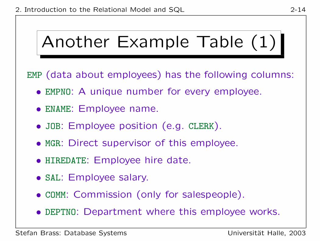
EMP (data about employees) has the following columns:
• EMPNO: A unique number for every employee.
• ENAME: Employee name.
• JOB: Employee position (e.g. CLERK).
• MGR: Direct supervisor of this employee.
• HIREDATE: Employee hire date.
• SAL: Employee salary.
• COMM: Commission (only for salespeople).
• DEPTNO: Department where this employee works.
Stefan Brass: Database Systems Universitat Halle, 2003

2. Introduction to the Relational Model and SQL 2-15
Another Example Table (2)
EMP
EMPNO ENAME JOB MGR HIREDATE SAL COMM DEPTNO
7369 SMITH CLERK 7902 17-DEC-80 800 20
7499 ALLEN SALESMAN 7698 20-FEB-81 1600 300 30
7521 WARD SALESMAN 7698 22-FEB-81 1250 500 30
7566 JONES MANAGER 7839 02-APR-81 2975 20
7654 MARTIN SALESMAN 7698 28-SEP-81 1250 1400 30
7698 BLAKE MANAGER 7839 01-MAY-81 2850 30
7782 CLARK MANAGER 7839 09-JUN-81 2450 10
7788 SCOTT ANALYST 7566 09-DEC-82 3000 20
7839 KING PRESIDENT 17-NOV-81 5000 10
7844 TURNER SALESMAN 7698 08-SEP-81 1500 0 30
7876 ADAMS CLERK 7788 12-JAN-83 1100 20
7900 JAMES CLERK 7698 03-DEC-81 950 30
7902 FORD ANALYST 7566 03-DEC-81 3000 20
7934 MILLER CLERK 7782 23-JAN-82 1300 10
Stefan Brass: Database Systems Universitat Halle, 2003

2. Introduction to the Relational Model and SQL 2-16
Foreign Keys (1)
• The relational model has no physical pointers.
• However, it has some kind of “logical pointer”.
• E.g., the column DEPTNO in the table EMP refers to
the table DEPT.
• Since DEPTNO is declared as a key in the table DEPT, a
department number uniquely identifies a single row
of DEPT.
• A value for DEPTNO can be seen as “logical address”
of a row in DEPT.
Stefan Brass: Database Systems Universitat Halle, 2003

2. Introduction to the Relational Model and SQL 2-17
Foreign Keys (2)
• By including a department number in EMP, each row
in EMP “points to” a row in DEPT.
• Of course, it is important that department numbers
in EMP also occur in DEPT.
• E.g. if EMP contains a row with DEPTNO = 70, this
would be a kind of “dangling pointer”.
Of course, the system does not crash as would be the case with physi-cal pointers: In SQL, rows are combined by comparing column values,and then this row would simply be ignored, because no matching rowin DEPT is found. But nevertheless, such a table entry is some kind oferror and should be excluded. This is the purpose of foreign keys.
Stefan Brass: Database Systems Universitat Halle, 2003

2. Introduction to the Relational Model and SQL 2-18
Foreign Keys (3)
• The relational model permits to declare DEPTNO as
a foreign key that references DEPT.
• Then a DBMS will refuse
� an insertion into EMP with a value for DEPTNO that
does not appear in DEPT,
� a deletion of a row in DEPT that is still referenced
by a row in EMP,
It might be possible to select that in this case all employees ofthe deleted department are recursively deleted, too.
� corresponding changes of DEPTNO values.
Stefan Brass: Database Systems Universitat Halle, 2003

2. Introduction to the Relational Model and SQL 2-19
Foreign Keys (4)
• The example table contains also a second foreign
key: The column MGR contains the employee number
of the employee’s direct supervisor.
• This shows that
� It is possible that a foreign key refers to another
row in the same table (or even the same row).
� The foreign key column and the referenced key
column can have different names.
Stefan Brass: Database Systems Universitat Halle, 2003

2. Introduction to the Relational Model and SQL 2-20
Null Values
• The relational model allows table entries to remain
empty (contain a “null value”).
• In the example table: Only salespeople have a com-
mission, the company president has no supervisor.
• In the schema declaration, one can specify for each
column whether it accepts null values or not.
• The null value is treated specially in comparisons.
See Chapter 5.
Stefan Brass: Database Systems Universitat Halle, 2003
2. Introduction to the Relational Model and SQL 2-21
Overview
1. The Relational Model, Example Database
2. Using SQL*Plus: First Demonstration
'
&
$
%3. Simple SQL Queries
4. Historical Remarks
Stefan Brass: Database Systems Universitat Halle, 2003

2. Introduction to the Relational Model and SQL 2-22
Oracle and SQL*Plus (1)
• SQL is the standard database language for relatio-
nal database management systems (RDBMSs).
Oracle supports SQL, as do all other modern RDBMS (e.g. DB2).The systems differ in many small details, see below.
• SQL*Plus is Oracle’s basic interface to the DBMS.
The DBMS itself (DB server) runs as a set of background processes,maybe on another machine in the network.
• E.g. C programs with embedded SQL also commu-
nicate with the Oracle server in SQL, but do not
use SQL*Plus.
Stefan Brass: Database Systems Universitat Halle, 2003

2. Introduction to the Relational Model and SQL 2-23
Oracle and SQL*Plus (2)
• The main task of SQL*Plus is
� to allow the user to enter SQL statements,
It provides some editing functions, e.g. to correct errors.
� send the query to the server, fetch the result,
� and print the output table.
It provides some control over output formatting.Simpler reports can be developed entirely in SQL*Plus.
• SQL*Plus also can process batch files (that contain
a sequence of commands). This is also supported
by a simple variable replacement mechanism.
Stefan Brass: Database Systems Universitat Halle, 2003

2. Introduction to the Relational Model and SQL 2-24
Basic Use of SQL*Plus (1)
• Under UNIX, enter the command “sqlplus”.
Environment variables must be set, especially ORACLE_HOME (e.g. to/oracle/OraHome1/), ORACLE_SID (database name, e.g. products), andpossibly ORACLE_BASE (e.g. to /oracle/OraHome1/), TWO_TASK (e.g. lxdb1),and of course PATH and possibly LD_LIBRARY_PATH. One can also setNLS_LANG to choose a language (e.g. GERMAN_GERMANY.WE8ISO8859P1).
• Under Windows, select SQL*Plus from the “Start”
Menu.
E.g. Start → Programme → Entwicklungsumgebungen → Oracle →Oracle-OraHome92 → Application Development → SQL Plus.
• SQL*Plus then asks for username and password.
Stefan Brass: Database Systems Universitat Halle, 2003

2. Introduction to the Relational Model and SQL 2-25
Basic Use of SQL*Plus (2)
• Many Oracle installations have a guest user “scott”
with password “tiger”.
For local databases, the “host string” field in the login box can usuallybe left empty. For a remote server, one must specify the server nameas defined e.g. in D:\software\Oracle9i\network\admin\tnsnames.ora.
Stefan Brass: Database Systems Universitat Halle, 2003

2. Introduction to the Relational Model and SQL 2-26
Basic Use of SQL*Plus (3)
• In Oracle, every user has his/her own DB schema.
• It is possible that two users have tables with the sa-
me name, but they are still distinct tables, because
they belong to different schemas.
Within an Oracle database, tables are identified by schema/user nameand table name. E.g. the table presidents of the user brass can bereferenced as “brass.presidents”. Of course, one can read or modifyit only if its owner (brass) has given the corresponding access rights.
• The example tables EMP, DEPT, etc. should already
be installed under the guest account scott.
Stefan Brass: Database Systems Universitat Halle, 2003

2. Introduction to the Relational Model and SQL 2-27
Basic Use of SQL*Plus (4)
• It is also possible to install a copy of the example
tables under one’s own account:
� Execute “demobld” from the UNIX or Windows
command prompt.It first tries to use a default user name (based on the OS account).If that does not work, an error message ist printed and the programasks for the correct Oracle user name and password.
� Or start SQL*Plus and enter:
“@D:\Software\Oracle9i\sqlplus\demo\demobld”The path depends on the installation. The file demobld.sql con-tains the SQL statements to create the tables and fill them withdata. The command “@x” executes the statements in x.sql.
Stefan Brass: Database Systems Universitat Halle, 2003

2. Introduction to the Relational Model and SQL 2-28
Basic Use of SQL*Plus (5)
• The SQL*Plus prompt is “SQL>”.
Or “2”, “3”, etc. for continuation lines.
• In SQL*Plus, SQL statements must end with “;”.
Alternative: “/” as the only contents of the next line.
• SQL statements can extend over several lines, and
SQL*Plus needs to know when the user is finished.
The “;” is not part of SQL. In DB2 and SQL server, the user mustinstead click on “execute” when the query is complete.
• SQL is not case sensitive (except in strings).
Stefan Brass: Database Systems Universitat Halle, 2003

2. Introduction to the Relational Model and SQL 2-29
Basic Use of SQL*Plus (6)
• To leave SQL*Plus, enter “exit” or “quit”.In contrast to SQL statements, such control commands need no semi-colon at the end. If they extend over multiple lines, each line (exceptthe last) must end with a hyphen “-”.
• The contents of a table can be listed with, e.g.:
SELECT * FROM EMP;
• The data dictionary table CAT (“catalog”) lists all
tables owned by the current user:
SELECT * FROM CAT;
• The columns of a table can be listed with, e.g.:
DESCRIBE EMP
Stefan Brass: Database Systems Universitat Halle, 2003

2. Introduction to the Relational Model and SQL 2-30
Basic Use of SQL*Plus (7)
Stefan Brass: Database Systems Universitat Halle, 2003

2. Introduction to the Relational Model and SQL 2-31
Basic Use of SQL*Plus (8)
UNIX> sqlplus. . . (Version and copyright information for SQL*Plus)
Enter user-name: scottEnter password: tiger (not visible)
. . . (Version information for the database server)
SQL> select * from dept;DEPTNO DNAME LOC
---------- -------------- -------------10 ACCOUNTING NEW YORK20 RESEARCH DALLAS30 SALES CHICAGO40 OPERATIONS BOSTON
Stefan Brass: Database Systems Universitat Halle, 2003

2. Introduction to the Relational Model and SQL 2-32
Basic Use of SQL*Plus (9)
• The last SQL command is still stored in a buffer.
It can be changed and re-executed.
E.g. in case of a syntax error.
• c/old/new (change) replaces the first occurrence of
“old” by “new”.
In the current line (line in which the error was detected).One can als write c/old/new/ or e.g. c!old!new.
• l (list) shows the contents of the buffer.
l3 shows only line 3 and makes it the current one.
• r (run) executes the contents of the buffer.
Stefan Brass: Database Systems Universitat Halle, 2003

2. Introduction to the Relational Model and SQL 2-33
Basic Use of SQL*Plus (10)
• edit writes the contents of the buffer to a file and
calls an editor.
The editor can be selected by the user, e.g. define _editor = vi. Thiscommand is only valid for the current session, but one can write itinto login.sql (in the current directory).
• It is also possible to write the SQL query into a
file, e.g. “x.sql”, and execute the file with @x.
E.g. you can keep an editor open in one window, write to the file,and execute the file in the other window, where you have SQL*Plusopen.
Stefan Brass: Database Systems Universitat Halle, 2003

2. Introduction to the Relational Model and SQL 2-34
Basic Use of SQL*Plus (11)
• It is important to clearly distinguish between
� SQL commands (queries, updates, etc.),
� SQL*Plus commands (e.g. exit, l, r, @x).
• SQL commands can extend over multiple lines and
must be closed with a “;” in SQL*Plus, whereas
SQL*Plus commands are single-line.
• If one accesses Oracle e.g. via Embedded SQL or
JDBC, the SQL*Plus extensions are not available.
Of course, they are also not available if one uses a different DBMS.
Stefan Brass: Database Systems Universitat Halle, 2003

2. Introduction to the Relational Model and SQL 2-35
Basic Use of SQL*Plus (12)
SQL> select *2 frm dept;
frm dept
ERROR at line 2:
ORA-00923: FROM keyword not found where expected
SQL> c/frm/from/2* from dept
SQL> r1 select *
2* from dept
Stefan Brass: Database Systems Universitat Halle, 2003

2. Introduction to the Relational Model and SQL 2-36
Basic Use of SQL*Plus (13)
• If the first keyword is misspelled, the command is
not stored in the buffer, and must be retyped.
Only SQL statements (recognized by first keyword) are stored in thebuffer, not SQL*Plus control commands.
• In SQL*Plus, the character “&” is used for marking
variables that are replaced by user input:
SQL> insert into DEPT
2 values (50, ’R&D’, ’Pittsburgh’);
Enter value for d:
Stefan Brass: Database Systems Universitat Halle, 2003

2. Introduction to the Relational Model and SQL 2-37
Basic Use of SQL*Plus (14)
• Oracle reports only one error in the SQL command.
There might be more errors.
The position which Oracle marks is not necessary the position wherethe error really is (no parser can do that). But it is also not necessarilythe first position where a parser could find an error.
• E.g. here quotes are missing around strings:
SQL> insert into DEPT values(60, WWW, Dallas);
insert into dept values(40, www, Dallas)
*ERROR at line 1:
ORA-00984: column not allowed here
Stefan Brass: Database Systems Universitat Halle, 2003

2. Introduction to the Relational Model and SQL 2-38
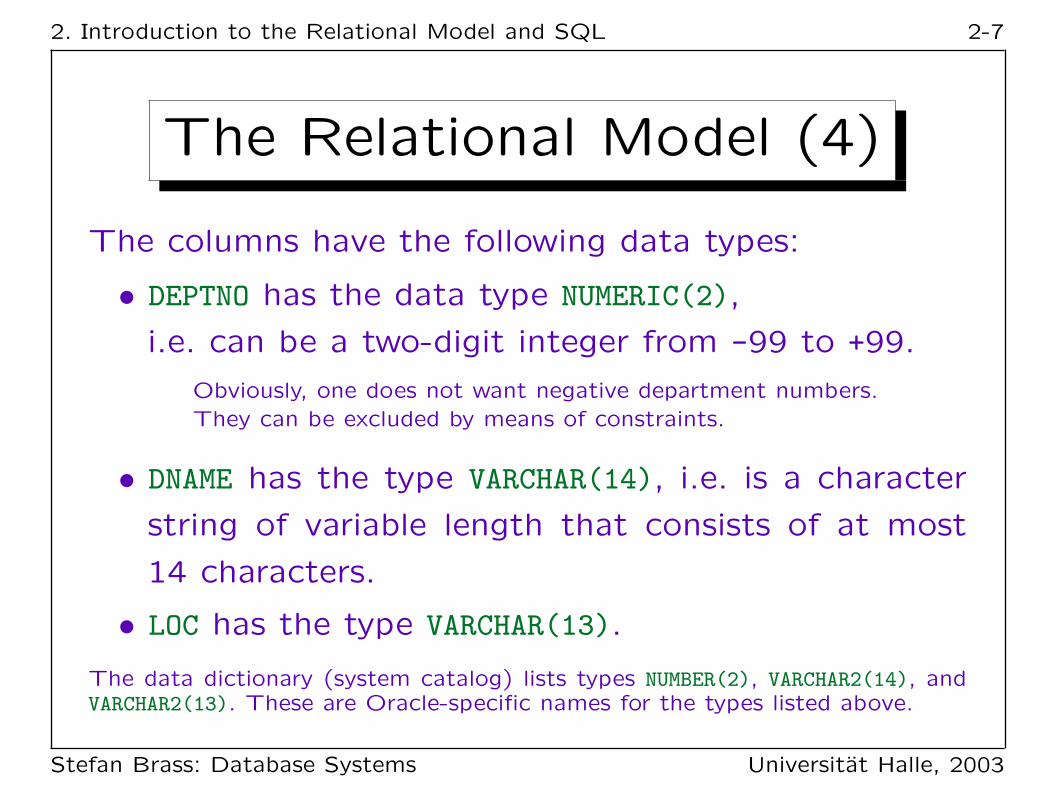
SQL*Plus Worksheet
• If one wants a bit more graphical interface, some
Oracle versions come with the SQL*Plus Works-
heet (part of the Oracle Enterprise Manager).
• The window is split into two parts:
� In the upper part one enters the query.
� In the lower part, the result is shown.
• The lightning button executes the query.
Stefan Brass: Database Systems Universitat Halle, 2003

2. Introduction to the Relational Model and SQL 2-39
Stefan Brass: Database Systems Universitat Halle, 2003

2. Introduction to the Relational Model and SQL 2-40
Overview
1. The Relational Model, Example Database
2. Using SQL*Plus: First Demonstration
3. Simple SQL Queries
'
&
$
%4. Historical Remarks
Stefan Brass: Database Systems Universitat Halle, 2003

2. Introduction to the Relational Model and SQL 2-41
Simple SQL Queries (1)
• Simple SQL queries have the structure
SELECT ... FROM ... WHERE ...
• After FROM list the table from which to extract data.
More than one table can be listed, see below.
• After WHERE specify conditions for the rows to be
selected.
The WHERE-clause can be missing, then all rows are selected.
• After SELECT define which columns to print.
“*” prints all columns.
Stefan Brass: Database Systems Universitat Halle, 2003

2. Introduction to the Relational Model and SQL 2-42
Simple SQL Queries (2)
• Show the entire department table:
SELECT * FROM DEPT
DEPTNO DNAME LOC
10 ACCOUNTING NEW YORK
20 RESEARCH DALLAS
30 SALES CHICAGO
40 OPERATIONS BOSTON
• Equivalent Solution:
SELECT DEPTNO, DNAME, LOC FROM DEPT
Stefan Brass: Database Systems Universitat Halle, 2003

2. Introduction to the Relational Model and SQL 2-43
Simple SQL Queries (3)
• SQL is not case-sensitive, except inside strings.All characters in an SQL command are turned into uppercase beforethey are processed (except inside quotes).To get a table or column name containing lower case letters, it mustbe enclosed in " (should be avoided).
• SQL is format-free (like Pascal, C, Java, etc.).Line breaks, spaces, and tabulator characters can be inserted betweenthe words (tokens) of an SQL command.
• Thus, the following query is the same as the pre-
vious one:select deptno, DName , loc
from dept
Stefan Brass: Database Systems Universitat Halle, 2003

2. Introduction to the Relational Model and SQL 2-44
Using Conditions (1)
• To get all data about the department in “DALLAS”:
SELECT * FROM DEPT WHERE LOC = ’DALLAS’
DEPTNO DNAME LOC
20 RESEARCH DALLAS
• String constants are marked by single quotes.
Double quotes are only used for delimited identifiers (column namescontaining lowercase characters etc.).
• Inside string constants, SQL is case-sensitive.
So the following will select 0 rows (empty result):
SELECT * FROM DEPT WHERE LOC = ’Dallas’
Stefan Brass: Database Systems Universitat Halle, 2003

2. Introduction to the Relational Model and SQL 2-45
Using Conditions (2)
• Print the name, job, and salary of all employees
who earn at least $2500:
SELECT ENAME, JOB, SAL
FROM EMP
WHERE SAL >= 2500
ENAME JOB SAL
JONES MANAGER 2975
BLAKE MANAGER 2850
SCOTT ANALYST 3000
KING PRESIDENT 5000
FORD ANALYST 3000
Stefan Brass: Database Systems Universitat Halle, 2003

2. Introduction to the Relational Model and SQL 2-46
Using Conditions (3)
• It is not necessary to output columns which are
used in the conditions.WHERE is evaluated before SELECT.
• E.g. print the employee number and name of all
managers:SELECT EMPNO, ENAME
FROM EMP
WHERE JOB = ’MANAGER’
EMPNO ENAME
7566 JONES
7698 BLAKE
7782 CLARK
Stefan Brass: Database Systems Universitat Halle, 2003

2. Introduction to the Relational Model and SQL 2-47
Pattern Matching (1)
• SQL also has an operator for “pattern matching”
of strings (allowing the use of “wildcards”).
• E.g. print number and name of all managers:SELECT EMPNO, ENAME
FROM EMP
WHERE JOB LIKE ’MANA%’
• “%” matches any sequence of arbitrary characters,
“_” matches any single character.
“%” corresponds to the “*” in the shell (command prompt),and “_” to “?”.
Stefan Brass: Database Systems Universitat Halle, 2003

2. Introduction to the Relational Model and SQL 2-48
Pattern Matching (2)
• LIKE must be used for pattern matching.
The equals sign only tests for literal equality.
Even if the comparison string contains “%” or “_”.
• E.g. the following is legal SQL, but will return the
empty result:
SELECT EMPNO, ENAME Wrong!FROM EMP
WHERE JOB = ’MANA%’
Stefan Brass: Database Systems Universitat Halle, 2003

2. Introduction to the Relational Model and SQL 2-49
Arithmetic Expressions
• SQL contains standard arithmetic expressions.
• E.g. print all employees who earn less than $15000
per year:SELECT ENAME
FROM EMP
WHERE SAL < 15000 / 12
ENAME
SMITH
ADAMS
JAMES
• The condition “SAL * 12 < 15000” is equivalent.
Stefan Brass: Database Systems Universitat Halle, 2003

2. Introduction to the Relational Model and SQL 2-50
Renaming Output Columns
• E.g. print the yearly salary of all managers:
SELECT ENAME, SAL * 12
FROM EMP
WHERE JOB = ’MANAGER’
ENAME SAL * 12
JONES 35700
BLAKE 34200
CLARK 29400
• To print the column heading “YEARLY_SALARY”:
SELECT ENAME, SAL * 12 YEARLY_SALARY ...
or SELECT ENAME, SAL * 12 AS YEARLY_SALARY ...
Stefan Brass: Database Systems Universitat Halle, 2003

2. Introduction to the Relational Model and SQL 2-51
Logical Connectives (1)
• AND, OR, NOT and parentheses “(”, “)” can be used
to construct more complicated conditions.
• E.g. print name and salary of all managers and the
president:SELECT ENAME, SAL
FROM EMP
WHERE JOB = ’MANAGER’ OR JOB = ’PRESIDENT’
• The query would not work with AND instead of OR.
The result would be empty (“0 rows selected”), since the JOB cannotbe “MANAGER” and “PRESIDENT” at the same time.
Stefan Brass: Database Systems Universitat Halle, 2003

2. Introduction to the Relational Model and SQL 2-52
Logical Connectives (2)
• The WHERE-condition is conceptionally evaluated for
every row of the table listed under FROM. If the result
is true, the SELECT-list is printed.
• An AND-condition is true if both parts are true,
an OR-condition is already true if one part is true:
C1 C2 C1 AND C2 C1 OR C2 NOT C1
False False False False TrueFalse True False True TrueTrue False False True FalseTrue True True True False
Stefan Brass: Database Systems Universitat Halle, 2003

2. Introduction to the Relational Model and SQL 2-53
Logical Connectives (3)
EMP
EMPNO ENAME JOB JOB=’MANAGER’ JOB=’PRESIDENT’
7369 SMITH CLERK False False
7499 ALLEN SALESMAN False False
7521 WARD SALESMAN False False
7566 JONES MANAGER True False
7654 MARTIN SALESMAN False False
7698 BLAKE MANAGER True False
7782 CLARK MANAGER True False
7788 SCOTT ANALYST False False
7839 KING PRESIDENT False True
7844 TURNER SALESMAN False False... ... ... ... ...
Stefan Brass: Database Systems Universitat Halle, 2003

2. Introduction to the Relational Model and SQL 2-54
Logical Connectives (4)
• Without parentheses, AND binds more strongly than
OR (and NOT binds even more strongly than AND).
• E.g. consider this query:SELECT ENAME, SAL Wrong!FROM EMP
WHERE JOB = ’MANAGER’ OR JOB = ’PRESIDENT’
AND SAL >= 3000
• The system will understand the condition as:
WHERE JOB = ’MANAGER’
OR (JOB = ’PRESIDENT’ AND SAL >= 3000)
Stefan Brass: Database Systems Universitat Halle, 2003

2. Introduction to the Relational Model and SQL 2-55
Removing Duplicates (1)
• Queries can produce duplicate rows.
• E.g. list all jobs:
SELECT JOB FROM EMP
• Since this query is processed by a loop over the em-
ployee table, in which the job of every employee is
printed, it will output the same job multiple times.
• Duplicate elimination can be requested by adding
the keyword DISTINCT after SELECT:
SELECT DISTINCT JOB FROM EMP
Stefan Brass: Database Systems Universitat Halle, 2003

2. Introduction to the Relational Model and SQL 2-56
Removing Duplicates (2)
• DISTINCT works on output rows, not single columns.
Specify it only once, even for multiple columns:
SELECT DISTINCT JOB, MGR
FROM EMP
• There is no way to print each job only once and
for every job the set of managers — that would be
a nested table (supported only in advanced NF2 or
object-relational DBMS).
In standard relational DBMS, each table entry is atomic. But outputformatting can give something similar. E.g. in SQL*Plus, it is possibleto suppress a column value if it is the same as in the preceding row.
Stefan Brass: Database Systems Universitat Halle, 2003

2. Introduction to the Relational Model and SQL 2-57
Sorting Output Rows (1)
• The sequence, in which the resulting rows are prin-
ted, is not predictable unless one requests sorting.
• E.g. print employee names and their salary, ordered
alphabetically by employee name:
SELECT ENAME, SAL
FROM EMP
ORDER BY ENAME
• The “ORDER BY” clause is purely cosmetic:
It does not change the query result in any way,
it only prints the result in a more readable fashion.
Stefan Brass: Database Systems Universitat Halle, 2003

2. Introduction to the Relational Model and SQL 2-58
Sorting Output Rows (2)
• One can also specify multiple sorting criteria.
Only useful if the main column for sorting contains duplicate values.
• E.g. print the employees who earn at least 2000
dollars, ordered by department number. For equal
department numbers, employees should be ordered
by descending salaries:
SELECT DEPTNO, ENAME, SAL
FROM EMP
WHERE SAL >= 2000
ORDER BY DEPTNO, SAL DESC
Stefan Brass: Database Systems Universitat Halle, 2003
2. Introduction to the Relational Model and SQL 2-59
Outlook: Joining Tables
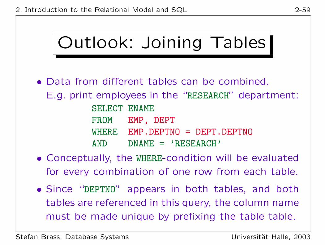
• Data from different tables can be combined.
E.g. print employees in the “RESEARCH” department:SELECT ENAME
FROM EMP, DEPT
WHERE EMP.DEPTNO = DEPT.DEPTNO
AND DNAME = ’RESEARCH’
• Conceptually, the WHERE-condition will be evaluated
for every combination of one row from each table.
• Since “DEPTNO” appears in both tables, and both
tables are referenced in this query, the column name
must be made unique by prefixing the table table.
Stefan Brass: Database Systems Universitat Halle, 2003

2. Introduction to the Relational Model and SQL 2-60
Exercises (1)
EMP
EMPNO ENAME JOB MGR HIREDATE SAL COMM DEPTNO
7369 SMITH CLERK 7902 17-DEC-80 800 20
7499 ALLEN SALESMAN 7698 20-FEB-81 1600 300 30
7521 WARD SALESMAN 7698 22-FEB-81 1250 500 30
7566 JONES MANAGER 7839 02-APR-81 2975 20
7654 MARTIN SALESMAN 7698 28-SEP-81 1250 1400 30
7698 BLAKE MANAGER 7839 01-MAY-81 2850 30
7782 CLARK MANAGER 7839 09-JUN-81 2450 10
7788 SCOTT ANALYST 7566 09-DEC-82 3000 20
7839 KING PRESIDENT 17-NOV-81 5000 10
7844 TURNER SALESMAN 7698 08-SEP-81 1500 0 30
7876 ADAMS CLERK 7788 12-JAN-83 1100 20
7900 JAMES CLERK 7698 03-DEC-81 950 30
7902 FORD ANALYST 7566 03-DEC-81 3000 20
7934 MILLER CLERK 7782 23-JAN-82 1300 10
Stefan Brass: Database Systems Universitat Halle, 2003

2. Introduction to the Relational Model and SQL 2-61
Exercises (2)
Please formulate the following queries in SQL:
• Who has employee number 7839 (King) as direct
supervisor?
• Who has a salary between $1000 and $2000? Print
name and salary and order the result by names.
“Between” is meant as including the two boundaries.
• Which employee names consist of exactly four cha-
racters?
Stefan Brass: Database Systems Universitat Halle, 2003
2. Introduction to the Relational Model and SQL 2-62
Exercises (3)
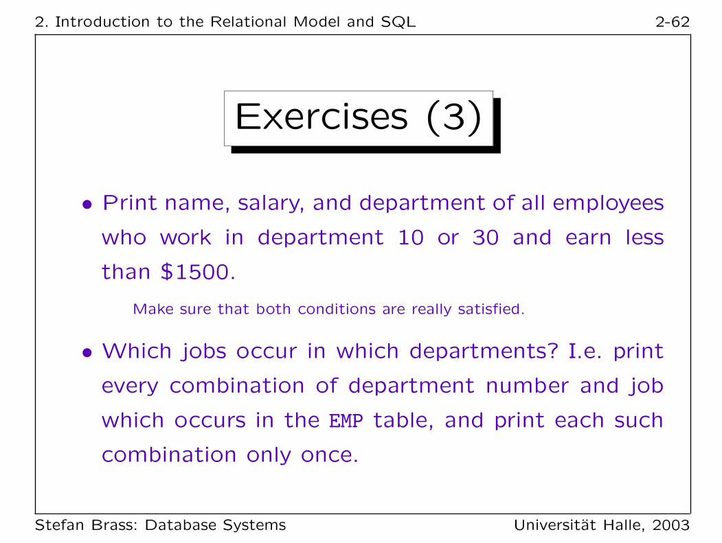
• Print name, salary, and department of all employees
who work in department 10 or 30 and earn less
than $1500.
Make sure that both conditions are really satisfied.
• Which jobs occur in which departments? I.e. print
every combination of department number and job
which occurs in the EMP table, and print each such
combination only once.
Stefan Brass: Database Systems Universitat Halle, 2003

2. Introduction to the Relational Model and SQL 2-63
Overview
1. The Relational Model, Example Database
2. Using SQL*Plus: First Demonstration
3. Simple SQL Queries
4. Historical Remarks
'
&
$
%
Stefan Brass: Database Systems Universitat Halle, 2003
2. Introduction to the Relational Model and SQL 2-64
Relational Model: History
• The relational model (RM) was proposed by
Edgar F. Codd (1970).It was the first data model that was theoretically defined prior toimplementation. Codd got the Turing Price in 1981.
• First Implementations (1976):
� System R (IBM)
� Ingres (Stonebraker, UC Berkeley).
• First commercial systems: Oracle (1979), Ingres
(1980?) and IBM SQL/DS (1981).
• Today “state of the art” in industry.
Stefan Brass: Database Systems Universitat Halle, 2003

2. Introduction to the Relational Model and SQL 2-65
Reasons for Success (1)
• Much simpler than earlier data models.
Only one concept: Finite relation (set of tuples).
• Easily understandable, even for non specialists:
Relations correspond to tables.
• Abstraction of known “files of records”.
• The relational model has set-oriented operations.
In earlier models, one had to navigate from one
record to the next.
Stefan Brass: Database Systems Universitat Halle, 2003

2. Introduction to the Relational Model and SQL 2-66
Reasons for Success (2)
• Declarative query language:
No need to think about efficient evaluation.
One only writes conditions for the required data. The DBMS con-tains a “query optimizer” that finds an efficient query evaluation plan(i.e. generates a good imperative program for evaluating the query).In earlier models, programmers had to think about the use of indexes(access paths) and many other details.
• The relational model has a solid theoretical foun-
dation. It is tightly connected to first-order logic.
Stefan Brass: Database Systems Universitat Halle, 2003

2. Introduction to the Relational Model and SQL 2-67
SQL
• Today, SQL is the only database language for re-
lational DBMSs (industry standard).
• SQL is used for:
� Interactive “ad-hoc” commands and
� application program development (embedded in-
to other languages like C, Java, HTML).
• SQL is based on a variant of first order logic called
tuple calculus.
But includes elements from relational algebra, too (e.g. UNION).It tries to be relatively near to natural language.
Stefan Brass: Database Systems Universitat Halle, 2003

2. Introduction to the Relational Model and SQL 2-68
History
• SEQUEL, an earlier version of SQL, was designed
by Chamberlin, Boyce et al. at IBM Research, San
Jose (1974).
SEQUEL stands for “Structured English Query Language”. Somepeople pronounce SQL this way. Others use “ess-cue-ell”. The namewas changed for legal reasons (SEQUEL was a registered trademark).Codd was also in San Jose when he invented the relational model.
• SQL was the language of System/R (1976/77).
System/R was a very influential research prototype.
• First commercial systems supporting SQL were
Oracle (1979) and IBM SQL/DS (1981).
Stefan Brass: Database Systems Universitat Halle, 2003

2. Introduction to the Relational Model and SQL 2-69
Standards
• First Standard 1986/87 (ANSI/ISO).
This was very late as there were already several SQL systems on themarket. The standard was the “smallest common denominator”. Itcontains only the common features of the existing implementations.
• Extension for foreign keys etc. in 1989 (SQL-89).
This version is called also SQL-1. All commercial implementationstoday support this standard, but each have significant extensions.
• Major Extension: SQL-2 or SQL-92 (1992).
Upward compatible to SQL-1. The standard defines three levels: “ent-ry”, “intermediate”, “full”. Oracle 8.0 and SQL Server 7.0 have onlyentry level conformance, but many extensions. SQL-92 is still theyardstick for RDBMSs.
Stefan Brass: Database Systems Universitat Halle, 2003

2. Introduction to the Relational Model and SQL 2-70
Future
• Current Standard: SQL-99.
SQL-99 is a preliminary version of the SQL-3 standard. Until 12/2000,the volumes 1–5 and 10 of the SQL-99 standard appeared. Theyhave together 2355 pages. The SQL-2 standard, which is not yetcompletely implemented, had only 587 pages.
• Some Features of SQL-3:
� User-defined data types, type constructors.
E.g. “LIST”, “SET”, “ROW” for structured attribute values.
� OO-Features (e.g. inheritance/subtables).
� Recursive queries.
� Triggers, Persistent Stored Modules.
Stefan Brass: Database Systems Universitat Halle, 2003