2. Introduction to BRILLOUIN spectroscopy · Scanning Brillouin microscopy Arch. Sci. Nat. Phys. Math. NS 46, Special volume 9 2. Introduction to BRILLOUIN spectroscopy BRILLOUIN

SCANNING BRILLOUIN MICROSCOPY Arch. Sci. Nat. Phys. Math. NS 46, volume spécial SCANNING BRILLOUIN MICROSCOPY Arch. Sci. Nat. Phys. Math. NS 46, volume spécialScanning Brillouin microscopy Arch. Sci. Nat. Phys. Math. NS 46, Special volume

9

2. Introduction to BRILLOUIN spectroscopy

BRILLOUIN spectroscopy is a well-established optical spectroscopic technique to

investigate mechanical as well as magnetic properties of matter (e.g. SANDERCOCK

1982, KRÜGER 1989, HILLEBRANDS 2005). The technique bases on the phenomenon

of inelastic laser light scattering, for which the incident photons are scattered by

thermally driven elementary excitations in matter, like sound waves (acoustic

phonons) or spin waves (magnons) (BRILLOUIN 1922, MANDELSTAM 1926, GROSS

1930, FABELINSKII 1968, CHU 1974, BERNE & PECORA 1976, DIL 1982). Note that

BRILLOUIN spectroscopy gives access to hypersonic waves and spin waves without

exciting them explicitly by transducers as necessary e.g. for ultrasonic pulse-echo

techniques. Since manifold introductory review articles and monographs on

BRILLOUIN scattering are available (FABELINSKII 1968, CHU 1974, BERNE & PECORA

1976, DIL 1982, SANDERCOCK 1982, KRÜGER 1989, HILLEBRANDS 2005) and since

the current article focuses on scanning BRILLOUIN microscopy, we give only a short

introduction to the theoretical background of BRILLOUIN scattering. In a first

reading, the sections marked with an asterisk* 2.1 (except figure 2.1 and the related

explications) and 2.4 can be skimmed over.

2.1. Scattering of laser light by thermally excited sound waves* The theory of inelastic scattering of visible light by thermally excited hypersonic

waves travelling through transparent matter will be recapitulated within a statistical

framework (CHU 1974, BERNE & PECORA 1976). Remember that indeed the

continuum of sound waves within condensed matter can be correlated to spatio-

temporal fluctuations of the mass density, or more generally, of the strain tensor

components (AULD 1973).

Consider a monochromatic laser beam that can be decomposed into planar waves,

incident on a dielectric sample. The electric part of each incident planar light wave

can be described as:

, (2.1)

Scanning Brillouin microscopy Arch. Sci. Nat. Phys. Math. NS 46, Special volume

8

2. Introduction to BRILLOUIN spectroscopy

BRILLOUIN spectroscopy is a well-established optical spectroscopic technique to

investigate mechanical as well as magnetic properties of matter (e.g. SANDERCOCK

1982, KRÜGER 1989, HILLEBRANDS 2005). The technique bases on the phenomenon

of inelastic laser light scattering, for which the incident photons are scattered by

thermally driven elementary excitations in matter, like sound waves (acoustic

phonons) or spin waves (magnons) (BRILLOUIN 1922, MANDELSTAM 1926, GROSS

1930, FABELINSKII 1968, CHU 1974, BERNE & PECORA 1976, DIL 1982). Note that

BRILLOUIN spectroscopy gives access to hypersonic waves and spin waves without

exciting them explicitly by transducers as necessary e.g. for ultrasonic pulse-echo

techniques. Since manifold introductory review articles and monographs on

BRILLOUIN scattering are available (FABELINSKII 1968, CHU 1974, BERNE & PECORA

1976, DIL 1982, SANDERCOCK 1982, KRÜGER 1989, HILLEBRANDS 2005) and since

the current article focuses on scanning BRILLOUIN microscopy, we give only a short

introduction to the theoretical background of BRILLOUIN scattering. In a first

reading, the sections marked with an asterisk* 2.1 (except figure 2.1 and the related

explications) and 2.4 can be skimmed over.

2.1. Scattering of laser light by thermally excited sound waves* The theory of inelastic scattering of visible light by thermally excited hypersonic

waves travelling through transparent matter will be recapitulated within a statistical

framework (CHU 1974, BERNE & PECORA 1976). Remember that indeed the

continuum of sound waves within condensed matter can be correlated to spatio-

temporal fluctuations of the mass density, or more generally, of the strain tensor

components (AULD 1973).

Consider a monochromatic laser beam that can be decomposed into planar

waves, incident on a dielectric sample. The electric part of each incident planar light

wave can be described as:

, (2.1)

11

SCANNING BRILLOUIN MICROSCOPY Arch. Sci. Nat. Phys. Math. NS 46, volume spécialScanning Brillouin microscopy Arch. Sci. Nat. Phys. Math. NS 46, Special volume

10

where denotes the wave vector in the medium, the position vector in the

sample’s coordinate system, the wave’s angular frequency, the electric field

amplitude and defines the direction of polarisation. For the sake of simplicity, we

assume that within anisotropic matter, the incident and scattered electromagnetic

waves represent eigenstates of the electromagnetic field. By this means we exclude

effects related to birefringence. The spatially and temporally fluctuating dielectric

properties of the sample are described by the dielectric tensor . If the

components of the dielectric tensor at optical frequencies fluctuate only spatially,

but not temporally, elastic light scattering can occur. In that case, the scattered

electromagnetic waves generally propagate along other directions than the incident

one while the energy is conserved: and , with denoting the

scattered wave vector. In the domain of materials science, typical candidates for

elastic light scattering processes are polycrystalline materials and nanocomposites

possessing optical heterogeneities in the 100 nanometer to micrometer range.

Inelastic light scattering occurs if the components of the dielectric tensor at optical

frequencies do not only fluctuate spatially, but also temporally. In this

context, two aspects need consideration: the spatially and temporally fluctuating

elementary excitations of the sample that couple to its optical properties and the

strength of this coupling. The spatio-temporal elementary excitations of the sample

can be divided into relaxational fluctuations, like fluctuations of the entropy, and

propagating fluctuations, like fluctuations of the mass density (BERNE & PECORA

1976). The corresponding modes are either diffusive or propagating ones. Sound

waves (also denoted as acoustic phonons) are generally induced by thermally

excited fluctuations of the strain tensor components, which degenerate in ideal

liquids to mass density fluctuations. The elasto-optical coupling between the strain

fluctuations and the optical fluctuations is described by the Pockels tensor (NYE

1972, VACHER & BOYER 1972). For most materials, the elasto-optical coupling for

shear strain is much weaker than that for longitudinal strain (NYE 1972, VACHER &

BOYER 1972).

The spatially and temporally fluctuating dielectric tensor at optical frequencies can

be described as:


9

where denotes the wave vector in the medium, the position vector in the

sample’s coordinate system, the wave’s angular frequency, the electric field

amplitude and defines the direction of polarisation. For the sake of simplicity, we

assume that within anisotropic matter, the incident and scattered electromagnetic

waves represent eigenstates of the electromagnetic field. By this means we exclude

effects related to birefringence. The spatially and temporally fluctuating dielectric

properties of the sample are described by the dielectric tensor . If the

components of the dielectric tensor at optical frequencies fluctuate only spatially,

but not temporally, elastic light scattering can occur. In that case, the scattered

electromagnetic waves generally propagate along other directions than the incident

one while the energy is conserved: and , with denoting the

scattered wave vector. In the domain of materials science, typical candidates for

elastic light scattering processes are polycrystalline materials and nanocomposites

possessing optical heterogeneities in the 100 nanometer to micrometer range.

Inelastic light scattering occurs if the components of the dielectric tensor at optical

frequencies do not only fluctuate spatially, but also temporally. In this

context, two aspects need consideration: the spatially and temporally fluctuating

elementary excitations of the sample that couple to its optical properties and the

strength of this coupling. The spatio-temporal elementary excitations of the sample

can be divided into relaxational fluctuations, like fluctuations of the entropy, and

propagating fluctuations, like fluctuations of the mass density (BERNE & PECORA

1976). The corresponding modes are either diffusive or propagating ones. Sound

waves (also denoted as acoustic phonons) are generally induced by thermally

excited fluctuations of the strain tensor components, which degenerate in ideal

liquids to mass density fluctuations. The elasto-optical coupling between the strain

fluctuations and the optical fluctuations is described by the Pockels tensor (NYE

1972, VACHER & BOYER 1972). For most materials, the elasto-optical coupling for

shear strain is much weaker than that for longitudinal strain (NYE 1972, VACHER &

BOYER 1972).

The spatially and temporally fluctuating dielectric tensor at optical

frequencies can be described as:

12


11

, (2.2)

with denoting the spatially and temporally averaged dielectric tensor and

the fluctuating part of the dielectric tensor. The transversely polarized

phonons are responsible for the off-diagonal entries of . The directions of

polarization of the incident planar light wave and of the chosen inelastically

scattered light wave yield the components according to:

. (2.3)

These dielectric fluctuations can be described by the spatio-temporal autocorrelation

function of , with V being the scattering volume and the considered time

interval:

(2.4)

The dynamic structure factor of the scattered light component travelling in

the -direction results from the spatio-temporal FOURIER transformation of the

autocorrelation function of :

, (2.5)

with

designating the acoustic phonon’s wave vector and

(with being the angular frequencies of the involved scattered

electric fields; see section 2.2) its angular frequency. The spectral power density

, which is closely related to the dynamic structure factor, is

experimentally accessible by BRILLOUIN spectroscopy. The factor depends on

the intensity of the incident light. As will be delineated below in a rough overview,

the BRILLOUIN lines of the spectral power density are intimately related to the

hypersonic properties of the sample, since these lines are due to dielectric

fluctuations induced by thermal fluctuations of the strain tensor components

(SOMMERFELD 1945, GRIMVALL 1986, LANDAU & LIFSHITZ 1991).

As described in KONDEPUDI & PRIGOGINE (1998), the thermally excited fluctuations

of the strain tensor components develop according to the same laws as macroscopic

deformations of small amplitude. Within the frame of linear response theory, the


10

, (2.2)

with denoting the spatially and temporally averaged dielectric tensor and

the fluctuating part of the dielectric tensor. The transversely polarized

phonons are responsible for the off-diagonal entries of . The directions of

polarization of the incident planar light wave and of the chosen inelastically

scattered light wave yield the components according to:

. (2.3)

These dielectric fluctuations can be described by the spatio-temporal autocorrelation

function of , with V being the scattering volume and the considered time

interval:

(2.4)

The dynamic structure factor of the scattered light component travelling in

the -direction results from the spatio-temporal FOURIER transformation of the

autocorrelation function of :

, (2.5)

with

designating the acoustic phonon’s wave vector and

(with being the angular frequencies of the involved scattered

electric fields; see section 2.2) its angular frequency. The spectral power density

, which is closely related to the dynamic structure factor, is

experimentally accessible by BRILLOUIN spectroscopy. The factor depends on

the intensity of the incident light. As will be delineated below in a rough overview,

the BRILLOUIN lines of the spectral power density are intimately related to the

hypersonic properties of the sample, since these lines are due to dielectric

fluctuations induced by thermal fluctuations of the strain tensor components

(SOMMERFELD 1945, GRIMVALL 1986, LANDAU & LIFSHITZ 1991).

As described in KONDEPUDI & PRIGOGINE (1998), the thermally excited

fluctuations of the strain tensor components develop according to the same laws as

macroscopic deformations of small amplitude. Within the frame of linear response

13


12

strain

can be related to the thermally excited fluctuating elastic force

density via the elastic susceptibility tensor , according to:

. (2.6)

Considering the storing and dissipative parts of the elastic interaction by the

symmetric forth rank tensors of the elastic moduli

and viscosities

(with k, l, m, n = 1, 2, 3), the strains evolve with time like

damped oscillators. The components of the inverse elastic susceptibilities

correspond to (LANDAU & LIFSHITZ 1991, KONDEPUDI & PRIGOGINE 1998):

, (2.7)

with denoting the mass density and the Kronecker symbol. The tensor

can be diagonalised in dependence of and , which results in:

(2.8)

with

(2.9)

where characterizes the polarization state of the sound wave and

denotes the effective elastic modulus for the given wave vector and polarization.

The three complex eigenfrequencies correspond to the

poles of equation (2.9) with:

(2.10)

and

. (2.11)

Here designates the acoustic damping and the

eigenfrequencies of the undamped sound waves for a given wave vector . The

related eigenvectors, i.e. the polarization vectors of the three sound waves, are

orthogonal to each other. For p=1, the mode is generally quasi-longitudinally

polarized: its polarization vector is almost collinear to the direction of propagation

(AULD 1973). Two quasi-transversely polarized modes are described by p=2 and

p=3. For elastically isotropic solids, all modes are purely longitudinally or


11

theory, the strain can be related to the thermally excited fluctuating elastic

force density via the elastic susceptibility tensor , according to:

. (2.6)

Considering the storing and dissipative parts of the elastic interaction by the

symmetric forth rank tensors of the elastic moduli

and viscosities

(with k, l, m, n = 1, 2, 3), the strains evolve with time like

damped oscillators. The components of the inverse elastic susceptibilities

correspond to (LANDAU & LIFSHITZ 1991, KONDEPUDI & PRIGOGINE 1998):

, (2.7)

with denoting the mass density and the Kronecker symbol. The tensor

can be diagonalised in dependence of and , which results in:

(2.8)

with

(2.9)

where characterizes the polarization state of the sound wave and

denotes the effective elastic modulus for the given wave vector and polarization.

The three complex eigenfrequencies correspond to the

poles of equation (2.9) with:

(2.10)

and

. (2.11)

Here designates the acoustic damping and the

eigenfrequencies of the undamped sound waves for a given wave vector . The

related eigenvectors, i.e. the polarization vectors of the three sound waves, are

orthogonal to each other. For p=1, the mode is generally quasi-longitudinally

polarized: its polarization vector is almost collinear to the direction of propagation

(AULD 1973). Two quasi-transversely polarized modes are described by p=2 and

p=3. For elastically isotropic solids, all modes are purely longitudinally or

14


13

transversely polarized, i.e. the propagation and polarization vectors are either

collinear or perpendicular (AULD 1973). Moreover, the two transversely polarized

modes are degenerated for isotropic solids. These shear modes do even not

propagate at all in ideal isotropic liquids, where the term ‘ideal’ implicates the

absence of viscoelastic behaviour. In contrast, if the acoustic modes couple to

molecular structural relaxations in a liquid, transversely polarized sound modes can

be detected at sufficiently high frequencies (CHU 1974, BERNE & PECORA 1976,

KRÜGER 1989).

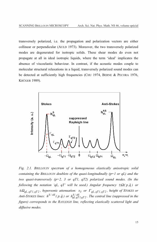
Fig. 2.1. BRILLOUIN spectrum of a homogeneous elastically anisotropic solid

containing the Brillouin doublets of the quasi-longitudinally (p=1 or qL) and the

two quasi-transversely (p=2, 3 or qT1, qT2) polarized sound modes. (In the

following the notation ‘qL, qT’ will be used.) Angular frequency or

, hypersonic attenuation: or , height of Stokes or

Anti-Stokes lines: or . The central line (suppressed in the

figure) corresponds to the RAYLEIGH line, reflecting elastically scattered light and

diffusive modes.


12

transversely polarized, i.e. the propagation and polarization vectors are either

collinear or perpendicular (AULD 1973). Moreover, the two transversely polarized

modes are degenerated for isotropic solids. These shear modes do even not

propagate at all in ideal isotropic liquids, where the term ‘ideal’ implicates the

absence of viscoelastic behaviour. In contrast, if the acoustic modes couple to

molecular structural relaxations in a liquid, transversely polarized sound modes can

be detected at sufficiently high frequencies (CHU 1974, BERNE & PECORA 1976,

KRÜGER 1989).

Fig. 2.1. BRILLOUIN spectrum of a homogeneous elastically anisotropic solid

containing the BRILLOUIN doublets of the quasi-longitudinally (p=1 or qL) and the

two quasi-transversely (p=2, 3 or qT1, qT2) polarized sound modes. (In the

following the notation ‘qL, qT’ will be used.) Angular frequency or

, hypersonic attenuation: or , height of STOKES or

Anti-STOKES lines: or . The central line (suppressed in the

figure) corresponds to the RAYLEIGH line, reflecting elastically scattered light and

diffusive modes.

15


14

In the classical limit, the fluctuation-dissipation theorem (KONDEPUDI & PRIGOGINE

1998) relates the polarization-independent dynamic structure factor to the

imaginary part of the susceptibility

by:

. (2.12)

Note that the opto-acoustic coupling is not part of the so-defined dynamic structure

factor, and therefore has to be accounted for by an appropriate prefactor.

In the present rough overview, the relationship between the experimentally

accessible spectral power density

and the elastic

susceptibilities, described by equation (2.12), permits us to sense that the angular

frequencies and attenuations

of the sound waves can be determined

from the measured BRILLOUIN spectrum. A typical BRILLOUIN spectrum for a

homogeneous anisotropic solid is given in figure 2.1. In the centre of the BRILLOUIN

spectrum appears the RAYLEIGH line, corresponding to the elastically scattered light

and the diffusive modes. The three BRILLOUIN doublets are positioned

symmetrically to the RAYLEIGH line on the horizontal angular frequency axis

. In order to calculate the intrinsic hypersonic attenuations the

instrumental broadening has to be deconvolved from the measured BRILLOUIN

spectrum. The angular frequency and attenuation correspond to the position and the

half width at half maximum of the BRILLOUIN lines, respectively. The statistical

error of the hypersonic angular frequency typically lies in the one-tenth of percent

regime, whereas that of the attenuation is larger by roughly a factor of 10. An

increasing half width at half maximum of the BRILLOUIN lines indicates a decreased

lifetime of the considered phonon mode . The here described lifetime of the

phonon (or temporal attenuation of a sound wave) and the spatial attenuation of a

sound wave known from ultrasonic investigations are related by the sound velocity.

For a very small temporal hypersonic attenuation, i.e. , the angular

frequency is not renormalized by the attenuation (see equation (2.11)). Several

16


15

mechanisms are known to contribute to the hypersonic attenuation, like structural

relaxation processes with their main relaxation frequencies in the GHz regime

(BERNE & PECORA 1976, KRÜGER 1989).

2.2. The kinematic approach

In the frame of a quantum-mechanical description, BRILLOUIN scattering results

from inelastic scattering of light photons by acoustic phonons. Applying the law of

conservation of energy to this scattering process allows one to relate the hypersonic

angular frequency of the phonons to the angular frequencies and of the

incident and scattered light, respectively, according to:

. (2.13)

The sign ‘+’ corresponds to the annihilation of phonons (Anti-STOKES scattering),

and the sign ‘-’ to the creation of phonons (STOKES scattering) (see figure 2.1 in

section 2.1). The energy transfer between an incident light photon and an acoustic

phonon equals to about of the photon’s energy. Since typical frequencies of

visible light are about , the angular frequencies of the involved acoustic

phonons are usually in the GHz regime. Similarly the law of conservation of

momentum relates the wave vector of the hypersonic wave to the wave vectors

and of the incident and scattered light according to:

. (2.14)

A schematic representation of this law is given in figure 2.2. Using the inner

scattering angle , the norm of the wave vector equals to:

. (2.15)

17


16

Due to the very small energy transfer between phonons and photons, is a

valid approximation leading to:

. (2.16)

If denotes the vacuum laser wavelength and n the sample’s refractive index, one

obtains:

. (2.17)

Note that in BRILLOUIN scattering the acoustic wave vector is selected by

adjusting the adequate scattering geometry, and that the phonon’s frequency is the

usually complex response. As elucidated in section 2.1, in general three acoustic

phonons, one quasi-longitudinally polarized and two quasi-transversely polarized

are determined for one selected wave vector in an elastically homogeneous solid

(AULD 1973).

Fig. 2.2. Schematic representation of momentum conservation during an inelastic

light scattering process. Sample represented in blue; , : incident/scattered

light wave vector within the sample; : wave vector of the acoustic phonon, and

: inner scattering angle.

For a typical vacuum laser wavelength of , the phonon wavelength

equals to some hundred nanometres and is hence of the same order of

magnitude as the laser wavelength. Thus, optical elastic scattering, like RAYLEIGH or

MIE scattering (BORN & WOLF 1999) in a heterogeneous sample is in most cases

accompanied by acoustic RAYLEIGH or MIE scattering (MORSE & INGARD 1968). For

18


17

sufficiently small hypersonic attenuation ( ), the phase velocity of the quasi-

longitudinally (qL) and quasi-transversely (qT) polarized acoustic modes depends

on the phonon wavelength and frequency f according to:

. (2.18)

Or, using equation (2.17):

. (2.19)

Knowing in addition the sample’s mass density, equation (2.19) allows the

calculation of the related elastic moduli (AULD 1973):

. (2.20)

2.3. Classical scattering geometries

Three common scattering geometries, defining the -vector involved in the

scattering process, are depicted in figure 2.3. In classical BRILLOUIN spectroscopy, a

typical scattering volume is about . The 90N scattering geometry, shown

in figure 2.3a, is a commonly used scattering geometry due to its easy alignment as

, where denotes the outer scattering angle (i.e. the angle between the

incident and scattered light beam outside the sample). Similarly easy to handle is the

backscattering geometry depicted in figure 2.3b, with . The

backscattering geometry is especially suitable in case of non-transparent samples as

the properties within the scattering volume can often still be probed close to the

sample’s surface. The major difference to the situation depicted in figure 2.3b is that

for a non-transparent sample the scattering volume is much more reduced in the x3-

direction (see also section 3.2). Note that in the backscattering geometry for

elastically isotropic samples only information about longitudinally polarized sound

waves can be gathered because of symmetry reasons (VACHER & BOYER 1972).

During the last years, the backscattering geometry has proven to be highly

promising for studying structural processes in dependence of time for transparent

19


18

materials (PHILIPP et al. 2009, 2011, SANCTUARY et al. 2010). Indeed, the large

scattering volume in the -direction allows for a comparatively high temporal

resolution as BRILLOUIN spectra can be recorded fast. Equations (2.17) and (2.18)

allow for calculating the phonon wavelengths and sound velocities for both

scattering geometries (using or , respectively). The related

values, both dependent on the sample’s refractive index, are indicated in table 2.1.

Fig. 2.3. Representation of (a) the 90N scattering geometry, (b) the backscattering

geometry, and (c) the scattering geometry (here: outer scattering angle

). Sample represented in blue, scattering volume in red. (1) laser beam

incident on the sample, (2) laser beam leaving the sample, (3) selected direction of

the inelastically scattered light emerging from the scattering volume. , :

incident and scattered wave vector, : wave vector of the acoustic phonon.

: sample coordinate system.

The scattering geometry, with being strictly between 0° and 90°, is

specifically adapted to many experimental challenges (e.g. KRÜGER et al. 1978a,

1981, 1986, KRÜGER 1989). It possesses the special attribute that the adjusted

phonon wave vector is independent of the sample’s refractive index n in case

of optically isotropic samples. Indeed, applying SNELL’s law to figure 2.3c allows

for expressing the inner scattering angle in dependence of the outer scattering

angle :

. (2.21)


17

materials (PHILIPP et al. 2009, 2011, SANCTUARY et al. 2010). Indeed, the large

scattering volume in the -direction allows for a comparatively high temporal

resolution as BRILLOUIN spectra can be recorded fast. Equations (2.17) and (2.18)

allow for calculating the phonon wavelengths and sound velocities for both

scattering geometries (using or , respectively). The related

values, both dependent on the sample’s refractive index, are indicated in table 2.1.

Fig. 2.3. Representation of (a) the 90N scattering geometry, (b) the backscattering

geometry, and (c) the scattering geometry (here: outer scattering angle

). Sample represented in blue, scattering volume in red. (1) laser beam

incident on the sample, (2) laser beam leaving the sample, (3) selected direction of

the inelastically scattered light emerging from the scattering volume. , :

incident and scattered wave vector, : wave vector of the acoustic phonon.

: sample coordinate system.

The scattering geometry, with being strictly between 0° and 90°, is

specifically adapted to many experimental challenges (e.g. KRÜGER et al. 1978a,

1981, 1986, KRÜGER 1989). It possesses the special attribute that the adjusted

phonon wave vector is independent of the sample’s refractive index n in case

of optically isotropic samples. Indeed, applying SNELL’s law to figure 2.3c allows

for expressing the inner scattering angle in dependence of the outer scattering

angle :

. (2.21)

20


19

Combining equations (2.19) and (2.21) then directly leads to the n-independent

sound velocity expression for the scattering geometry given in table 2.1.

Because of the usually small birefringence of anisotropic samples, the expressions

indicated in table 2.1 are also high quality approximations for the phonon wave

vector and the sound velocities of optically anisotropic samples, with absolute errors

being usually smaller than 0.1% (KRÜGER et al. 1986). Hence, this scattering

geometry is especially useful if high precision acoustic data are needed for samples

of unknown optical properties. For instance it is frequently employed for

temperature dependent measurements of samples with an unknown refractive index

evolution versus temperature (e.g. KRÜGER 1989, KRÜGER et al. 1990, 1994,

JIMÉNEZ RIOBÓO et al. 1990, PHILIPP et al. 2008). As thoroughly described in

chapter 3, this scattering geometry is often combined with angle-resolved

BRILLOUIN spectroscopy to precisely determine the elastic tensor properties of

anisotropic samples. Commonly, an outer scattering angle of is chosen

because of the easy alignment. The corresponding scattering geometry is called the

90A scattering geometry.

Table 2.1. Expressions for the phonon wavelength and the sound velocity

for different scattering geometries for optically isotropic samples.

Scattering

geometry

90N backscattering 90A

Phonon

wavelength

Sound velocity


19



















Scattering

geometry


Phonon

wavelength

Sound velocity


19



















Scattering

geometry


Phonon

wavelength

Sound velocity

21


20

2.4. Determination of elastic tensor components for

anisotropic matter*

Scanning acoustic microscopy applied to inhomogeneous and heterogeneous

anisotropic materials only makes sense if in addition to the spatial variations of

elastic properties accompanying local symmetry changes are recorded. Otherwise

both effects, i.e. spatial symmetry changes and inherent elastic modulus variations,

can hardly be discriminated. A purposeful experimental approach consists in the

combination of scanning BRILLOUIN microscopy with angle-resolved BRILLOUIN

spectroscopy. First a recapitulation of the determination of the elastic modulus

tensor is proposed before proceeding to this combined experimental technique in the

next section.

As shown in the previous sections, in BRILLOUIN spectroscopy the adjustment of the

scattering geometry permits to select a phonon wave vector with a desired

direction and norm. Angle-resolved BRILLOUIN spectroscopy allows a comparably

easy access to the elastic properties in a given scattering volume for many

differently oriented ’s within one plate-like sample (e.g. KRÜGER et al. 1985,

1986, 1990, 1994, 2001). Furthermore, in a homogeneous anisotropic material, this

technique yields for a given phonon wave vector at best three sound velocities

(AULD 1973). The term ‘at best’ means that the opto-acoustic coupling coefficients

must be so large that sufficiently intense phonon lines appear in the BRILLOUIN

spectrum. For a given the related phonon modes are orthogonally polarized, but

these polarizations are usually neither purely longitudinal nor purely transversal.

The evaluation of a BRILLOUIN spectrum does not immediately lead to the material-

describing elastic susceptibility, i.e. the fourth rank elastic modulus tensor.

For moderate or negligible acoustic losses this problem is solved by combining the

constituting CHRISTOFFEL equation (AULD 1973) with a statistically representative

dataset of measured sound velocities (KRÜGER et al. 1986, KRÜGER 1989).

The CHRISTOFFEL equation combines the measured with the components of

the elastic modulus matrix (VOIGT notation; AULD 1973):


19

2.4. Determination of elastic tensor components for

anisotropic matter*

Scanning acoustic microscopy applied to inhomogeneous and heterogeneous

anisotropic materials only makes sense if in addition to the spatial variations of

elastic properties accompanying local symmetry changes are recorded. Otherwise

both effects, i.e. spatial symmetry changes and inherent elastic modulus variations,

can hardly be discriminated. A purposeful experimental approach consists in the

combination of scanning BRILLOUIN microscopy with angle-resolved BRILLOUIN

spectroscopy. First a recapitulation of the determination of the elastic modulus

tensor is proposed before proceeding to this combined experimental technique in the

next section.

As shown in the previous sections, in BRILLOUIN spectroscopy the

adjustment of the scattering geometry permits to select a phonon wave vector

with a desired direction and norm. Angle-resolved BRILLOUIN spectroscopy allows a

comparably easy access to the elastic properties in a given scattering volume for

many differently oriented ’s within one plate-like sample (e.g. KRÜGER et al.

1985, 1986, 1990, 1994, 2001). Furthermore, in a homogeneous anisotropic

material, this technique yields for a given phonon wave vector at best three sound

velocities (AULD 1973). The term ‘at best’ means that the opto-acoustic coupling

coefficients must be so large that sufficiently intense phonon lines appear in the

BRILLOUIN spectrum. For a given the related phonon modes are orthogonally

polarized, but these polarizations are usually neither purely longitudinal nor purely

transversal. The evaluation of a BRILLOUIN spectrum does not immediately lead to

the material-describing elastic susceptibility, i.e. the fourth rank elastic modulus

tensor.

For moderate or negligible acoustic losses this problem is solved by

combining the constituting CHRISTOFFEL equation (AULD 1973) with a statistically

representative dataset of measured sound velocities (KRÜGER et al. 1986,

KRÜGER 1989). The CHRISTOFFEL equation combines the measured with the

components of the elastic modulus matrix (VOIGT notation; AULD

1973):

22


21

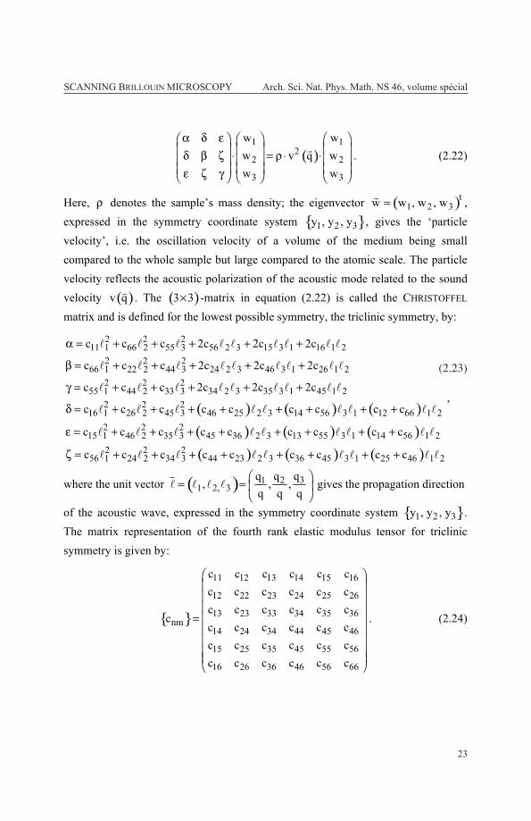
. (2.22)

Here, denotes the sample’s mass density; the eigenvector ,

expressed in the symmetry coordinate system , gives the ‘particle

velocity’, i.e. the oscillation velocity of a volume of the medium being small

compared to the whole sample but large compared to the atomic scale. The particle

velocity reflects the acoustic polarization of the acoustic mode related to the sound

velocity . The -matrix in equation (2.22) is called the CHRISTOFFEL

matrix and is defined for the lowest possible symmetry, the triclinic symmetry, by:

,

where the unit vector gives the propagation direction

of the acoustic wave, expressed in the symmetry coordinate system .

The matrix representation of the fourth rank elastic modulus tensor for triclinic

symmetry is given by:

. (2.24)

23

(2.23)


22

For cubic symmetry the CHRISTOFFEL matrix significantly simplifies and is

expressed as follows:

. (2.25)

The three-dimensional sound velocity polar diagram for crystals of cubic symmetry

is still a three-sheeted hypersuperface, similar to the lower symmetries (AULD 1973,

KRÜGER et al. 1986, KRÜGER 1989). This is in contrast to the degenerated optical

phase velocity surface for crystals of cubic symmetry.

Fig. 2.4. Differently oriented symmetry coordinate systems with

respect to the sample coordinate system . The blue face denotes a plane

parallel to the -plane.

The combination of the 90A scattering geometry with angle-resolved BRILLOUIN

spectroscopy is especially suited for determining the elastic tensor of low-symmetry

transparent anisotropic materials; a task which is hardly possible by other

experimental techniques (e.g. KRÜGER et al. 1990, 1994, 2001). A prerequisite for

this method is the availability of plate-like samples of the same material, each

having a differently oriented symmetry coordinate system with respect


21

For cubic symmetry the CHRISTOFFEL matrix significantly simplifies and is

expressed as follows:

. (2.25)

The three-dimensional sound velocity polar diagram for crystals of cubic symmetry

is still a three-sheeted hypersuperface, similar to the lower symmetries (AULD 1973,

KRÜGER et al. 1986, KRÜGER 1989). This is in contrast to the degenerated optical

phase velocity surface for crystals of cubic symmetry.

Fig. 2.4. Differently oriented symmetry coordinate systems with

respect to the sample coordinate system . The blue face denotes a plane

parallel to the -plane.

The combination of the 90A scattering geometry with angle-resolved

BRILLOUIN spectroscopy is especially suited for determining the elastic tensor of

low-symmetry transparent anisotropic materials; a task which is hardly possible by

other experimental techniques (e.g. KRÜGER et al. 1990, 1994, 2001). A prerequisite

for this method is the availability of plate-like samples of the same material, each

having a differently oriented symmetry coordinate system with respect

24


23

to the sample coordinate system (see figure 2.4). As elucidated in the

next chapter, rotating the sample plate around an axis being normal to the sample

plane and confining the phonon wave vector within this plane yields the acoustic

indicatrix of this sample cut (KRÜGER et al. 1985, 1986). The determination of the

acoustic indicatrices for a suitable choice of different crystal cuts provides a

representative set of elastic data sufficient to calculate, on the base of the

CHRISTOFFEL equation, the components of the elastic modulus tensor. This will be

exemplarily illustrated in chapter 4 for several crystalline materials.

25

Documents

2. Introduction to BRILLOUIN spectroscopy · Scanning Brillouin microscopy Arch. Sci. Nat. Phys. Math. NS 46, Special volume 9 2. Introduction to BRILLOUIN spectroscopy BRILLOUIN