15

2 Hertz Potentials

2.1 Introduction

A general feature of classical electrodynamics is the fact that anelectromagnetic field must be a solution of Maxwell's equations. Thereforemany theoretical considerations on the structure of Maxwell's equationsexist. The analysis of an electromagnetic field is often facilitated by the useof auxiliary functions known as potential functions (scalar, vectorial,tensorial) [1, p.23]. These are solutions of partial differential equations. Thepartial differential equations are such, that solving them for the potentialfunctions is equivalent to the more tedious task of solving Maxwell'sequations directly [2].

The most elegant approach to this is the field representation in terms ofGreen's tensors. However, this treatment has the fundamentaldisadvantage that tensor differential equations have to be solved. It is onlyfor special kinds of media that Green's tensors can be reduced to scalarGreen's functions [2].

It was shown by Hertz that an arbitrary electromagnetic field in a (sourcefree) homogeneous linear isotropic medium can be defined in terms of asingle vector potential

�

∏ [1, p.28]. The Hertz vector potential notation is anefficient mathematical formalism for solving electromagnetic problems. Aswill be shown, Hertz vector potential can be reduced to a set of two scalarpotentials, which are solutions of Helmholtz’s equations, for any orthogonalcurvilinear coordinate system. These solutions are independent only in thecase of an isotropic medium [2]. Note that at present the Hertz potentialnotation has been extended in order to take into account sources containedin the medium [1, pp. 30-32 & pp. 430-431]. However, this can not be donein a straightforward manner. The current and charge densities first need tobe expressed in terms of an electric polarization vector

�

P using the

formulas: �

�

J Pt

= ∂∂

and ρ = −∇ ⋅� �

P .

A lot of present day textbooks on the subject of electromagnetism relyheavily on the magnetic vector potential

�

A and the scalar potential φ , alsooften called the mixed potential method. The main advantage of thismethod is the fact that the two Helmholtz’s equations that result from it (onevectorial and one scalar), directly take into account any current or chargesources lying in the medium. This is in contrast with the Hertz vectorpotential method where, as has been explained in the previous paragraph,the scalar potentials are more closely connected to the field intensities

�

Eand

�

H.

16

The magnetic vector potential �

A and the scalar potential φ are related to

the Hertz vector potential as follows [1, pp. 28-29]: �

�

At

= ∏µε ∂∂

and

φ = −∇ ⋅∏� �

, provided that �

A is defined by � � �

B A= ∇ × and not � � �

H A= ∇ × .(The latter definition is more common in East European countries.)

The big strength of the Hertz vector potential method lies with the fact thatthere is no need to check whether the solutions of the two scalar partialdifferential equations are solutions of the posed problem. This is clearly notthe case with the mixed potential method [3, p. 679]. For problems situatedin source free media, this property of the Hertz vector potential method faroutweighs the advantages of any other method. This also explains why, inthis text, the Hertz vector potential method is preferred over the mixedpotential method.

In recent years, a lot of research effort went into the development ofpotential formulations for anisotropic, gyrotropic, chiral and spatiallyinhomogeneous media [2]. For a detailed discussion on scalar Hertzpotentials for bigyrotropic media see [4].

17

2.2 Hertz's Wave Equation for Source Free HomogeneousLinear Isotropic Media

Assuming ej tω time dependence, Hertz's wave equation for a source freehomogeneous linear isotropic medium, independent of the coordinatesystem, is [3, p. 729]∇ ∏+ ∏ =2 2 0

� �

k (1)where ( )∇ ≡ ∇ ∇ ⋅ − ∇ × ∇ ×2 �

� �

�

� �

�

v v v (�

v is any vector) [1, p. 25], [3, p. 95]

and ( )k j j j2 2= − + = −ωµ σ ωε εµω ωµσ .(k is the complex wave number of the surrounding medium.)

Hertz's wave equation for source free homogeneous linear isotropic media(1) has two types of independent solutions:

�

∏ e and �

∏m .

These result in independent sets of E-type waves( )

� � �

H j e= + ∇ × ∏σ ωε , (2a)

( )� � � � �

E k e e= ∏ +∇ ∇ ⋅∏2 , (2b)

and H-type waves, respectively [3, p. 729]� � �

E j m= − ∇ × ∏ωµ , (3a)

( )� � � � �

H k m m= ∏ +∇ ∇ ⋅∏2 . (3b)

Note that throughout this text, permittivity ε will be treated as a complex quantity with twodistinct loss contributions [5]

ε ε ε σω

= ′ − ′′ −j j

where − ′′jε is the loss contribution due to molecular relaxation

and − j σω

is the conduction loss contribution. (The conductivity σ is measured at DC.)

However, in practice it is not always possible to make this distinction. This is often the casewith metals and good dielectrics. In those cases all losses can be treated as though beingentirely due to conduction or molecular relaxation, respectively.

Above relations follow from

( )� � � � � �

∇ × = + = ′ − ′′ +H j D J j j E Eω ω ε ε σ .

The loss tangent of a dielectric medium is defined by

tanδ ωε σωε

≡ ′′ +′

.

Permeability µ has only one loss contribution due to hysteresis: µ µ µ= ′ − ′′j .

18

2.3 Hertz's Wave Equation in Orthogonal CurvilinearCoordinate Systems with Two Arbitrary Scale Factors

Consider a right-hand orthogonal curvilinear coordinate system withcurvilinear coordinates ( )u u u1 2 3, , . Scale factor h1 equals one and scalefactors h2 and h3 can be chosen arbitrary.

(A detailed explanation of what curvilinear coordinates and scale factors are, can be foundin [1, pp. 38-59] and [6, pp. 124-130], together with definitions of gradient, divergence, curland Laplacian for such coordinate systems.)

Hertz's vector wave equation for source free homogeneous linear isotropicmedia (1) can be reduced to a scalar wave equation [3, pp. 729-730] bymaking use of the definitions given in [1, pp. 49-50]

∂∂

∂∂

∂∂

∂∂

∂∂

2

12

2 3 2

3

2 2 2 3 3

2

3 3

21 1 0∏ + ∏

+

∏

+ ∏ =

u h h uhh u h h u

hh u

k (4)

with ( )�

�

∏ = ∏ u u u e1 2 3 1, , . (5)�

e1 is in the unit vector in the u1-direction.

The field components of the E-type waves are obtained by introducing (5)into (2a+b)

E kue

e1

22

12= ∏ +∏∂∂

; H1 0= ,

Eh u u

e2

2

2

1 2

1=∏∂

∂ ∂;

( )H

jh u

e2

3 3

=+ ∏σ ωε ∂

∂, (6)

Eh u u

e3

3

2

1 3

1=∏∂

∂ ∂;

( )H

jh u

e3

2 2

= −+ ∏σ ωε ∂

∂.

The field components of the H-type waves are obtained by introducing (5)into (3a+b)

H kum

m1

22

12= ∏ +∏∂∂

; E1 0= ,

Hh u u

m2

2

2

1 2

1=∏∂

∂ ∂; E j

h um

23 3

= −∏ωµ ∂∂

, (7)

Hh u u

m3

3

2

1 3

1=∏∂

∂ ∂; E j

h um

32 2

=∏ωµ ∂∂

.

As can be seen from (7) and (8), E-type waves have no H-component in theu1-direction, whereas H-type waves have no E-component in that direction.By choosing appropriate values for h2 and h3, expressions for the fieldcomponents in Cartesian, cylindrical (including parabolic and elliptic) andeven spherical coordinate systems can be obtained.The more general case with three arbitrary scale factors gives rise to aninsoluble set of interdependent equations [1, pp. 50-51].

19

2.4 Hertz's Wave Equation in a Cartesian Coordinate System

The three scale factors h1, h2 and h3 all equal one in a right-hand Cartesiancoordinate system ( )u u u1 2 3, , . Hence, Hertz's vector wave equation (4)simplifies to∂∂

∂∂

∂∂

2

12

2

22

2

32

2 0∏ + ∏ + ∏ + ∏ =u u u

k (8)

with ( )�

�

∏ = ∏ u u u e1 2 3 1, , . (9)�

e1 is the unit vector in the u1-direction.

Therefore, the field components of the E-type waves are

E kue

e1

22

12= ∏ +∏∂∂

; H1 0= ,

Eu u

e2

2

1 2

=∏∂

∂ ∂; ( )H j

ue

23

= +∏

σ ωε∂∂

, (10)

Eu u

e3

2

1 3

=∏∂

∂ ∂; ( )H j

ue

32

= − +∏

σ ωε∂∂

.

The field components of the H-type waves are

H kum

m1

22

12= ∏ +∏∂∂

; E1 0= ,

Hu u

m2

2

1 2

=∏∂

∂ ∂; E j

um

23

= −∏

ωµ∂∂

, (11)

Hu u

m3

2

1 3

=∏∂

∂ ∂; E j

um

32

=∏

ωµ∂∂

.

20

2.5 Hertz's Wave Equation for a 2D-Uniform Guiding Structure

Propagation along a guiding structure occurs in one direction only. In thistext, the x-axis is chosen to be parallel with the propagation direction.Therefore, the waves along a uniform guiding structure have only an

( )e j t xxω β− -dependence in that direction. This means that Hertz vectorpotentials for two-dimensional uniform guiding structures are of the form[3, p. 800]

( )�

�

∏ = −F y z e ej xx, β1

where �

e1 can be either in the x-, y- or z-direction

and phase constant β β βγ

x x xxjj

= ′ − ′′ = .

The propagation of electromagnetic waves is usually characterized in terms of thepropagation constant γ α β= + j , where α is called the attenuation constant.

The formulation for β used in this text, is consistent with the expression for γ , namely( )γ β β β β β α= ′ − ′′ = ′′ + ′ ⇒ ′′ ≡j j j .

There exist a large number of 2D-uniform guiding structures, some of the best knownexamples are: the parallel wire line, coaxial cable, waveguide, strip line, microstrip line, slotline and the coplanar line.

Since ∂∂

β2

22∏ = − ∏

x x , Hertz's scalar wave equation (8) becomes

∂∂

∂∂

2

2

2

22 0∏ + ∏ + ∏ =

y zs (12)

where s k jx x2 2 2 2 2= − = − −β εµω ωµσ β . (13)

Solutions to (12) can readily be found by separation of the variables.Namely, let ( ) ( )∏ = −Y y Z z e j xxβ . (14)

Substituting (14) into (12) and dividing by (14) gives1 1 0

2

2

2

22

Yd Ydy Z

d Zdz

s+ + = .

Since the last term in the above equation is independent of both y and z,the first two terms need to be this as well.Therefore,1 2

22

Yd Ydy

sy= − ; 1 2

22

Zd Zdz

sz= − and s s sy z2 2 2+ = . (15)

21

The first two equations in (15) are linear homogeneous second orderdifferential equationsd Ydy

s Yy

2

22 0+ = ; d Z

dzs Zz

2

22 0+ = .

Hence, suitable Hertz potential solutions for two-dimensional uniformguiding structures are of the form [6, p. 105]

[ ] [ ]∏ = + ⋅ + ⋅+ − + − −c e c e c e c e ejs y js y js z js z j xy y z z x1 2 3 4

β , or equally,

( ) ( )[ ] ( ) ( )[ ]∏ = + ⋅ + ⋅ −c s y c s y c s z c s z ey y z zj xx

5 6 7 8cos sin cos sin β .

22

2.6 Hertz's Wave Equation in a Circular Cylindrical CoordinateSystem

In a cylindrical coordinate system, the scale factors are generally differentfrom one, except for the scale factor associated with the symmetry axis,usually called the z-axis. In order to apply expression (4), the scale factor h1should equal one. Therefore, let u z1 = .

The special case of a right-hand circular cylindrical coordinate system( )r z, ,φ gives u z1 = ; u r2 = and u3 = φ . (16)

The differential line element d� in a circular cylindrical coordinate system( )r z, ,φ is [7]

d dr r d dz� = + +2 2 2 2φ .

The scale factors are hence [6, p. 124]

hz1 1= =∂∂� ; h

r2 1= =∂∂� and h r3 = =∂

∂φ� . (17)

Substitute (16) and (17) into (4) to get∂∂

∂∂

∂∂

∂∂φ

∂∂φ

221 1 1 0∏ + ∏

+ ∏

+ ∏ =

z r rr

r r rk (18)

with ( )�

�

∏ = ∏ z r ez, ,φ . (19)

Propagation in cylindrical symmetric transmission lines occurs in onedirection only, which is usually along the z-axis. This means that theexpression for the Hertz vector potentials simplifies to

( )�

�

∏ = −F r e ej zz

z,φ β .

Since ∂∂

β2

2∏ = − ∏z z , Hertz’s scalar wave equation (18) becomes

1 1 1 02

r rr

r r rs∂

∂∂∂

∂∂φ

∂∂φ

∏

+ ∏

+ ∏ = (20)

where s k jz z2 2 2 2 2= − = − −β εµω ωµσ β . (21)

Solutions to (20) can readily be found by separation of the variables.Namely, let ( ) ( )∏ = −R r e j zzΦ φ β . (22)

Substituting (22) into (20) and dividing by (22) results in [3, p. 739]1 1 1 1 1 02

R rddr

r dRdr r

dd r

dd

s

+

+ =

ΦΦ

φ φ. (23)

23

Multiplying (23) by r2 givesrR

ddr

r dRdr

dd

s r

+ + =1 0

2

22 2

ΦΦφ

. (24)

Equation (24) can be separated using a separation constant n into1 2

22

ΦΦd

dn

φ= − , (25)

rR

ddr

r dRdr

s r nr

+ =2 2 2 (26)

where s s kr z2 2 2 2= = − β .

Equation (25) is a linear homogeneous second order differential equationdd

n2

22 0Φ Φ

φ+ = .

Solutions for Φ are of the form [6, p. 105]Φ = ++ −c e c ejn jn

1 2φ φ , or equally, (27a)( ) ( )Φ = +c n c n3 4cos sinφ φ . (27b)

Rewriting equation (26) results in an expression which can be recognizedas Bessel’s equation of order n [6, p. 106]rR

ddr

r dRdr

s r nr

+ − =2 2 2 0

⇒ + ⋅

+ − =r

Rr d R

drdRdr

s r nr

2

22 2 21 0

( )⇒ + + − =r d Rdr

r dRdr

s r n Rr2

2

22 2 2 0 (28)

with n ≥ 0 .

Solutions to Bessel’s equation of order n (28) are of the form [6, p. 106],[8, pp. 97-88]

( ) ( )R c J s r c Y s rn r n r= +5 6 , or equally, (29a)

( ) ( )R c H s r c H s rn r n r= +71

82( ) ( ) . (29b)

These solutions are linearly independent only if n is a positive integer.

At this point, Hertz’s scalar wave equation for circular cylindrical coordinatesystems (20) is solved. It suffices to substitute any form of (27) and (29)into (22) to obtain the Hertz potential solutions.

24

Substituting (16) and (22) into (6) gives the field components of the E-typewaves expressed in terms of a Hertz potential [3, p.740]E sz r e= ∏2 ; Hz = 0 ,

E jrr z

e= −∏

β∂∂

; ( )

Hj

rre=

+ ∏σ ωε ∂∂φ

, (30)

E jrz e

φβ ∂

∂φ= −

∏ ; ( )H jr

eφ σ ωε

∂∂

= − +∏ .

Likewise, substitute (16) and (22) into (7) to obtain the field components ofthe H-type wavesH sz r m= ∏2 ; Ez = 0,

H jrr z

m= −∏

β∂∂

; E jrr

m= −∏ωµ ∂∂φ

, (31)

H jrz m

φβ ∂

∂φ= −

∏ ; E jr

mφ ωµ

∂∂

=∏ .

25

2.7 Conclusions

Chapter 2 gave a review of Hertz potential theory. The convenience ofexpressing source free electromagnetic fields in terms of Hertz potentialswas clearly demonstrated. The theory is kept as general as possible,making it useful as a reference while solving many other electromagneticproblems.

2.8 References

[1] J. A. Stratton, Electromagnetic Theory, McGraw-Hill, 1941[2] W. Weiglhofer, "Scalarisation of Maxwell's equations in general

inhomogeneous bianisotropic media," IEE Proceedings, Vol. 134, Pt. H,No. 4, August 1987, pp. 357-360

[3] K. Simonyi, Theoretische Elektrotechnik, Johann Ambrosius Barth, 10.Auflage, 1993, (in German)

[4] W. Weiglhofer and W. Papousek, “Skalare Hertzsche Potentiale füranisotrope Medien,” Archiv für Elektronik und Übertragungstechnik, Vol.39, No. 6, Nov.-Dec. 1985, pp. 343-346, (in German)

[5] R. E. Collin, Foundations for Microwave Engineering, McGraw-Hill, 2nd

Ed., 1992, p. 26[6] M. R. Spiegel, Mathematical Handbook of Formulas and Tables,

Schaum’s Outline Series, McGraw-Hill, 1968[7] Joseph A. Edminister, Electromagnetics, Schaum’s Outline Series,

McGraw-Hill, 2nd Ed., 1993, p. 5[8] R. E. Collin, Field Theory of Guided Waves, IEEE Press, 2nd Ed., 1991

26

3 Plane Surface Waves along Plane Layers of Isotropic Media

3.1 Definition

A plane surface wave is defined as a plane wave that propagates along aplane interface of two different media without radiation [1, p.5].Note that radiation in this context is construed as being energy convertedfrom the surface wave field to some other field form.

Plane surface waves are inhomogeneous waves because the field is notconstant along surfaces of constant phase. In fact, in the case of a surfacewave the field decays exponentially over the wavefront with increase ofdistance from the surface.

There are E-type and H-type surface waves. The field of an E-type planesurface wave is depicted in Figure 3.1. For an H-type wave the E- and H-fields are interchanged and one of the fields is reversed in sign. Explicitequations for the fields of plane surface waves along various structures willbe derived rigorously later in this chapter.

x

zy

Figure 3.1: The field of an E-type plane surface wave

�

E

�

H

Medium 2

Medium 1

27

3.2 Plane Surface Waves and the Brewster Angle Phenomenon

There are many ways to explain the mechanism of surface waves. In themid-fifties Barlow et al. introduced the concept of surface impedance forthis purpose [1, pp. 15-17], [2], which will be explained in a later section.Earlier work by Zenneck (1907) associated plane surface waves with theBrewster angle phenomenon [1, pp. 29-33], [3, p. 697-701]. For this reasonplane surface waves are sometimes also called Zenneck waves. Due to themany prevailing misconceptions, the relation between plane surface wavesand the Brewster angle will receive some further attention here.

The Brewster angle is the angle of incidence at which a plane wave incidenton a plane material interface is totally transmitted (i.e. without reflection)from one medium, called medium 2 here, into another medium, calledmedium 1. Both media are assumed to be half spaces. In lossless media,the Brewster angle phenomenon only occurs for perpendicular and parallelpolarized incident plane waves. (The terms “perpendicular” and “parallel”refer to the orientation of the electric field intensity vector

�

Ei of the incidentplane wave with respect to the plane of incidence.) The Brewster angle isdifferent for the two types of polarization. From Fresnel’s equations [4], itcan be shown that the Brewster angle for perpendicular polarized incidentplane waves is

θ

ε µε µ

µµ

B a⊥ =−

−

sin1

1

1 2

2 1

2

1

2 and

θ

ε µε µ

εε

B a// sin=−

−

1

1

2 1

1 2

2

1

2

for parallel polarized incident plane waves.

Above equations result in a complex value for the Brewster angle:– if, for perpendicular polarization, µ µ2 1> ,– or if, for parallel polarization, ε ε2 1> ,– or if at least one of the two media has losses.

The physical meaning of a complex angle of incidence is an inhomogeneous planewave (which in fact very much resembles a surface wave) incident at that angle [1,p. 30], [3, p. 717], [5]. When the Brewster angle is complex, the angle for whichthe magnitude of the reflection coefficient is a minimum, is called the pseudo-Brewster angle [1, p. 31]. The Brewster angle is also sometimes called thepolarizing angle since a wave with both perpendicular and parallel componentsand which is incident at the Brewster angle will produce a reflected wave with onlya perpendicular or parallel component [6, p. 617]. To summarize, the onlyconnection between surface waves and the Brewster angle lies in the fact that theinhomogeneous wave required by a complex Brewster angle resembles a surfacewave.

28

3.3 Plane Surface Waves, Total Reflection and Leaky Waves

An idea of what the different fields along a material interface may look like,can be obtained by employing ray-optics theory once again. The existenceof propagating plane surface waves along a coated perfectly conductingplane, for example, can be explained with the help of the total reflectionphenomenon as shown in Figure 3.2.

yx

z

Figure 3.2: A ray-optics explanation for the propagation of plane surfacewaves along a coated perfectly conducting plane

Total reflection only occurs when a wave from medium 1 impinges uponmedium 2 at an angle of incidence θ1i equal to or exceeding the criticalangle θc and then only if medium 1 is more “dense” than medium 2 (k1>k2).

An expression for the critical angle as a function of k1 and k2 can beobtained as follows. The relation between the angles of reflection andrefraction is given by Snell’s law ( ) ( )k kt i2 2 1 1⋅ = ⋅sin sinθ θ

( ) ( )⇒ =sin sinθ θ21

21t i

kk

.

There will be no refracted wave if ( )sin θ2t is greater than one or

equivalently, if ( ) ( )sin sinθ θ12

1i c

kk

> = .

Hence, θc a kk

=

sin 2

1

.

σ = +∞

θ θ1i c>

θ 2t

k k1 2>

k 2

Medium 1

Medium 2

29

As suggested in Figure 3.2, total reflection can be accompanied by asurface wave propagating in medium 1, parallel with the material interface.What is not shown, is the fact that a surface wave field most of the timesalso extends into medium 2. This will be proven in the next section. Notethat a surface wave can exist along a coated perfectly conducting planeonly if the coating (medium 1) is more dense than the upper half space(medium 2) (k1>k2). If this is not the case or if the angle of incidence θ1i issmaller than the critical angle θc , part of the wave in medium 1 will betransmitted into medium 2 with each partial reflection. Therefore, the fieldwill quickly attenuate in the x-direction. The resulting inhomogeneous planewave is called a leaky wave and propagates away from the interface (Fig.3.3b).

Figure 3.3: (a) A surface wave, (b) a leaky wave (Medium 2 is assumed tobe loss free in this figure.)

Note that �

α 2 is perpendicular to �

β2 only if medium 2 is loss free(Im(k2) = 0). This will be shown now.

( ) ( )k k k j jx z x x z z22

22

22

2 22

2 22= + = − + −β α β α

( ) ( )⇒ = + − + − +k jx z x z x x z z22

22

22

22

22

2 2 2 22β β α α α β α β .Only and only if Im(k2) = 0 ⇒ + =α β α β2 2 2 2 0x x z z

⇒ ⋅ = ⇒ ⊥�

�

�

�

α β α β2 2 2 20 .

For the sake of simplicity, �

α 2 will always be drawn for the case wheremedium 2 is loss free, i.e. perpendicular to

�

β2 . However, the theorydeveloped in this text equally applies for lossy upper media.

Leaky waves violate the radiation condition since they only may exist ifpower is delivered to medium 1 from outside, in a direction towards thematerial interface with medium 2. This can be achieved by replacing theperfectly conducting plane in Figure 3.2 by the outer wall of a slottedwaveguide. It also important to know that a leaky wave can not be exitedby a plane wave incident from medium 2. In such a case, the result will be astanding wave in medium 2.

�

α 2

�

α 2

�

β 2

�

β 2

x

z

(b)(a)Equiphase Planes

Equiamplitude Planes

Medium 2

Medium 1 Medium 1

Medium 2

30

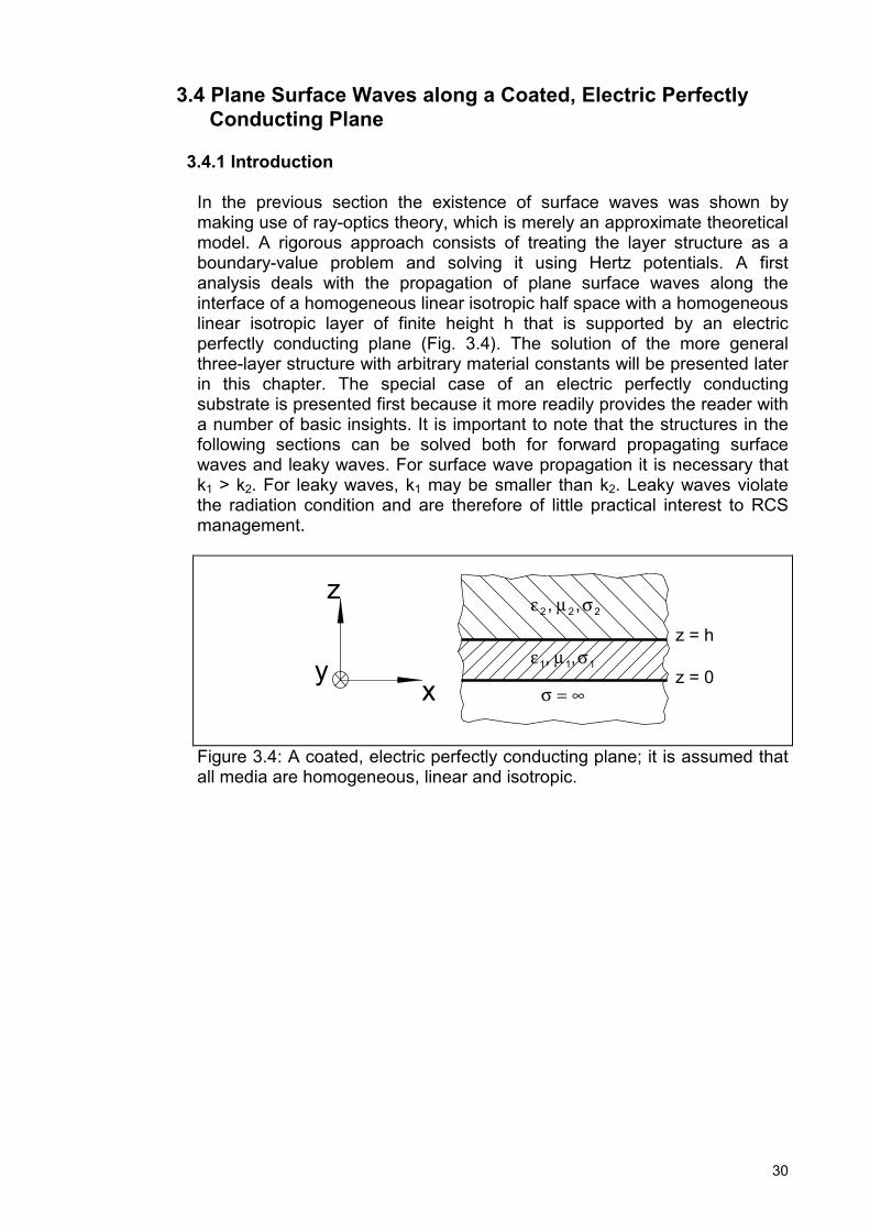
3.4 Plane Surface Waves along a Coated, Electric PerfectlyConducting Plane

3.4.1 Introduction

In the previous section the existence of surface waves was shown bymaking use of ray-optics theory, which is merely an approximate theoreticalmodel. A rigorous approach consists of treating the layer structure as aboundary-value problem and solving it using Hertz potentials. A firstanalysis deals with the propagation of plane surface waves along theinterface of a homogeneous linear isotropic half space with a homogeneouslinear isotropic layer of finite height h that is supported by an electricperfectly conducting plane (Fig. 3.4). The solution of the more generalthree-layer structure with arbitrary material constants will be presented laterin this chapter. The special case of an electric perfectly conductingsubstrate is presented first because it more readily provides the reader witha number of basic insights. It is important to note that the structures in thefollowing sections can be solved both for forward propagating surfacewaves and leaky waves. For surface wave propagation it is necessary thatk1 > k2. For leaky waves, k1 may be smaller than k2. Leaky waves violatethe radiation condition and are therefore of little practical interest to RCSmanagement.

yx

z

Figure 3.4: A coated, electric perfectly conducting plane; it is assumed thatall media are homogeneous, linear and isotropic.

ε µ σ2 2 2, ,

ε µ σ1 1 1, ,

σ = ∞z = 0

z = h

31

It is obvious that the Cartesian coordinate system (Section 2.4) is bestsuited for the analysis of plane waves. Assuming plane wave propagation inthe x-direction, the structure of Figure 3.4 can be treated as a special caseof a 2D-uniform guiding structure (see Section 2.5). Here however, none ofthe field components can have a y-dependence due to the fact that bothmedia are infinite in the y-direction. Hence, the Hertz vector potential

�

∏ willhave no y-dependence. Note that a field vector can still have componentsin the y-direction. For reasons that will be explained later,

�

∏ needs to bechosen in the z-direction.

A general expression for a Hertz vector potential having above-mentionedproperties is

( )�

�

∏ = ∏ −z e ej xz

xβ . (1)

In order to be able to apply (2.10) and (2.11), the relation between thecurvilinear coordinates and the Cartesian coordinates must be as followsu z1 = ; u x2 = and u y3 = .

32

Substituting (1) into (2.10) results in general expressions for the fieldcomponents of E-type waves within a medium

E kzz e

e= ∏ +∏2

2

2

∂∂

; Hz = 0 ,

E jzx x

e= −∏

β∂

∂; ( )H j

yxe= +

∏=σ ωε

∂∂

0 , (2)

Ez yy

e=∏

=∂∂ ∂

2

0 ; ( )H j jy x e= + ∏β σ ωε .

From (2) it can be seen that E-type plane surface waves are:1) longitudinal section magnetic (LSM) waves; the magnetic field intensity

�

H has no component in the direction normal to the material interface( )Hz = 0 and

2) transversal magnetic (TM) waves; the magnetic field intensity �

H has nocomponent in the propagation direction ( )Hx = 0 .

Substituting (1) into (2.11) leads to general expressions for the fieldcomponents of H-type waves within a medium

H kzz m

m= ∏ +∏2

2

2

∂∂

; Ez = 0,

H jzx x

m= −∏

β∂

∂; E j

yxm= −

∏=ωµ

∂∂

0 , (3)

Hz yy

m=∏

=∂∂ ∂

2

0 ; Ey x m= ∏β ωµ .

It can be concluded from (3) that H-type plane surface waves are:1) longitudinal section electric (LSE) waves; the electric field intensity

�

Ehas no component in the direction normal to the material interface( )Ez = 0 and

2) transversal electric (TE) waves; the electric field intensity �

E has nocomponent in the propagation direction ( )Ex = 0 .

33

3.4.2 E-Type Plane Surface Waves along a Coated, Electric PerfectlyConducting Plane

A suitable Hertz function for medium 1 that satisfies the boundary conditionE at zx = =0 0is ( )∏ = −

1 1 1A s z ezj xxcos β . (4)

The factor ( )cos s zz1 may be interpreted as a standing wave in the z-direction.

Introducing (4) into (2) results in( ) ( )E A k s s z ez z z

j xx1 1 1

21

21= − −cos β , (5a)

( )E j A s s z ex x z zj xx

1 1 1 1= −β βsin , (5b)Ey1 = 0 , (5c)Hz1 0= , (5d)Hx1 0= , (5e)

( ) ( )H j j A s z ey x zj xx

1 1 1 1 1= + −β σ ωε βcos . (5f)

Recalling (2.13)s k s kz x z x1

212 2

1 12 2= − ⇒ = + −β β . (6)

It is only for a matter of convenience that sz1 is chosen to equal the positivesquare root. Choosing the negative square root would have no effect on theresults.

A suitable Hertz function for medium 2 that satisfies the boundary condition� � �

E H when z= = → +∞0is ( )∏ = − − −

2 22A e ejs z h j xz xβ . (7)

The factor ( )e js z hz− −2 may be interpreted as a wave propagating in thepositive z-direction with phase constant s s jsz z z2 2 2= ′ − ′′ . Contrary to (6), thesign of sz2 is of importance here because sz2 belongs to the argument of anexponential function and therefore determines whether the solutions will beforward propagating surface waves or leaky waves. For surface waves,

′′ > ⇒ <s sz z2 20 0Im( ) , which corresponds to a decaying field in the positivez-direction. If on the other hand Im( )sz2 0> , the wave is a leaky wave. Inthat case the radiation condition is violated because the field in medium 2increases exponentially away from the interface.

34

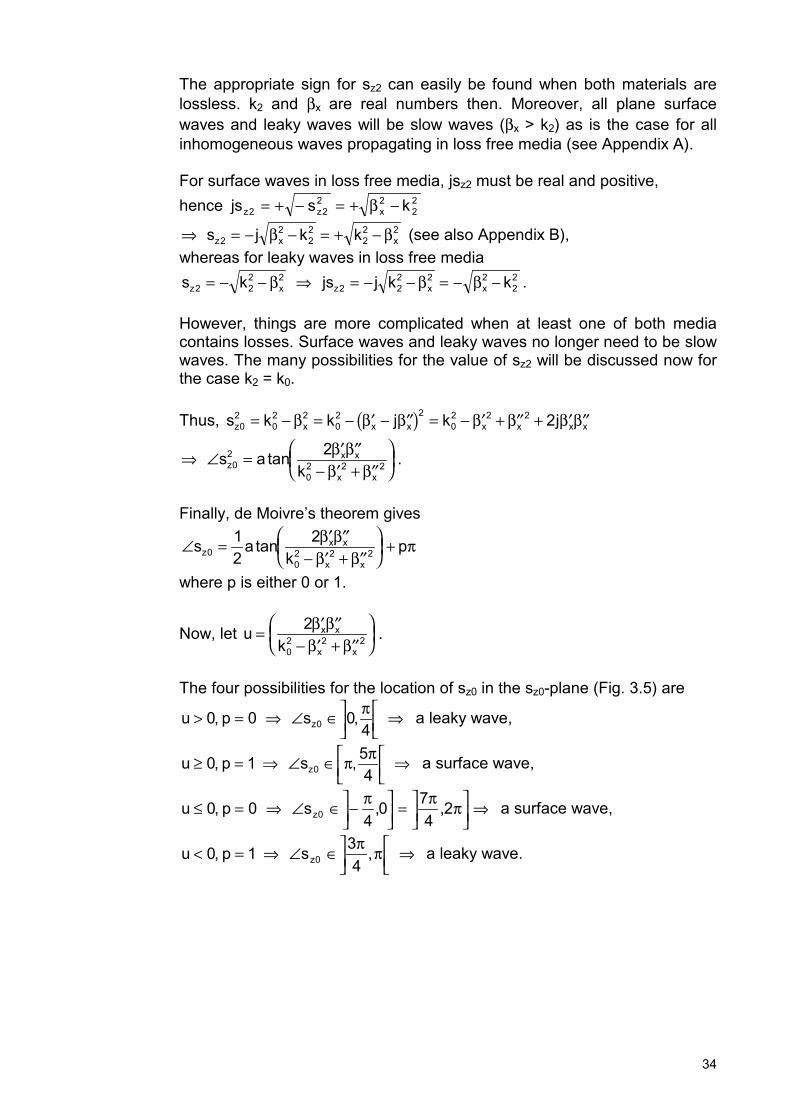
The appropriate sign for sz2 can easily be found when both materials arelossless. k2 and βx are real numbers then. Moreover, all plane surfacewaves and leaky waves will be slow waves (βx > k2) as is the case for allinhomogeneous waves propagating in loss free media (see Appendix A).

For surface waves in loss free media, jsz2 must be real and positive,hence js s kz z x2 2

2 222= + − = + −β

⇒ = − − = + −s j k kz x x22

22

22 2β β (see also Appendix B),

whereas for leaky waves in loss free medias k js j k kz x z x x2 2

2 22 2

2 2 222= − − ⇒ = − − = − −β β β .

However, things are more complicated when at least one of both mediacontains losses. Surface waves and leaky waves no longer need to be slowwaves. The many possibilities for the value of sz2 will be discussed now forthe case k2 = k0.

Thus, ( )s k k j k jz x x x x x x x02

02 2

02 2

02 2 2 2= − = − ′ − ′′ = − ′ + ′′ + ′ ′′β β β β β β β

⇒ ∠ = ′ ′′− ′ + ′′

s a

kzx x

x x0

2

02 2 2

2tan β ββ β

.

Finally, de Moivre’s theorem gives

∠ = ′ ′′− ′ + ′′

+s a

kpz

x x

x x0

02 2 2

12

2tan β ββ β

π

where p is either 0 or 1.

Now, let uk

x x

x x

= ′ ′′− ′ + ′′

202 2 2

β ββ β

.

The four possibilities for the location of sz0 in the sz0-plane (Fig. 3.5) are

u p sz> = ⇒ ∠ ∈

⇒0 0 040, , π a leaky wave,

u p sz≥ = ⇒ ∠ ∈

⇒0 1 540, ,π π a surface wave,

u p sz≤ = ⇒ ∠ ∈ −

=

⇒0 04

0 74

20, , ,π π π a surface wave,

u p sz< = ⇒ ∠ ∈

⇒0 1 340, ,π π a leaky wave.

35

Figure 3.5: The complex sz0-plane

Slow surface waves with moderate losses will most often fall into the thirdcategory. Equation (8a) gives rise to surface wave solutions as long asu k kx x x x≤ ⇔ − ′ + ′′ ≤ ⇔ ′′ ≤ − ′0 00

2 2 2 202 2β β β β

where k andx x0, ′ ′′β β are all positive real numbers.Even surface wave absorbers will almost always meet this requirement.This is shown by the numerical examples presented later in this chapter.However, to remain as general as possible, surface wave solutions are onlyobtained by letting ( )Re jsz2 0≥ or

( )js sign k kz x x22

22 2

22= −

−Re β β . (8a)

To obtain leaky wave solutions, let

( )js sign k kz x x22

22 2

22= − −

−Re β β . (8b)

Introducing (7) into (2) leads to( ) ( )E A k s e ez z

js z h j xz x2 2 2

22

2 2= − − − − β , (9a)( )E A s e ex x z

js z h j xz x2 2 2

2= − − − −β β , (9b)Ey2 0= , (9c)Hz2 0= , (9d)Hx2 0= , (9e)

( ) ( )H j j A e ey xjs z h j xz x

2 2 2 22= + − − −β σ ωε β . (9f)

∠sz0

sz0

Re(sz0)

Im(sz0)

SurfaceWaves

LeakyWaves

36

The tangential components of both �

E and �

H are continuous across theinterface of two media and thereforeE E at z hx x1 2= =

( )⇒ =A s s h jA sz z z1 1 1 2 2sin , (10)

as well as H H at z hy y1 2= =

( ) ( ) ( )⇒ + = +σ ωε σ ωε1 1 1 1 2 2 2j A s h j Azcos . (11)

Note that (10) and (11) would have resulted in a set of contradictoryequations, if

�

∏m e, were chosen in any direction other than the z-direction.

Dividing (10) by (11) yields

( )sj

s h jsj

zz

z1

1 11

2

2 2σ ωε σ ωε+=

+tan . (12)

Substituting (6) and (8a) into (12) results in the following expression for E-type surface waves

( ) ( )kj

h ksign k k

jx

x

x x12 2

1 112 2

222 2

22

2 2

−+

− =−

−

+β

σ ωεβ

β β

σ ωεtan

Re. (13)

This equation is transcendental and can therefore only be solvednumerically for β x . It is called a dispersion equation because it expressesthe nonlinear frequency dependence of β x . Both equation (12) and (13) areexpressions for the transverse resonance condition which requires thesame value for the longitudinal wave impedance looking straight down tothe interface (z = h) (14) as for the longitudinal wave impedance lookingstraight up [7, p. 12-6]. Hence, there will be no reflection in the equivalenttransmission line of the layer structure (Fig. 3.7).

Looking straight down from medium 2 to the interface, the longitudinalsurface impedance is (for a definition see Section 5.3.2)

Z EH

E z hH z h

jsj

j jsjs

t

x

y

z z�

�= − = − ==

= −+

=−

2

2

2

2 2

2

2 2

( )( ) σ ωε ωε σ

. (14)

The minus sign in (14) originates from the fact that the Poynting vector� � �

S E Hx y= ×2 2 is in the positive z-direction, whereas Zs� is the surfaceimpedance at the interface, looking in the negative z-direction.

The value of the transversal surface impedance is undefined.

37

3.4.3 H-Type Plane Surface Waves along a Coated, Electric PerfectlyConducting Plane

A suitable Hertz function for medium 1 that satisfies the boundary conditionE at zy = =0 0is ( )∏ = −

1 1 1A s z ezj xxsin β . (15)

The factor ( )sin s zz1 may be interpreted as a standing wave in the z-direction.

Introducing (15) into (3) results in( ) ( )H A k s s z ez z z

j xx1 1 1

21

21= − −sin β , (16a)

( )H j A s s z ex x z zj xx

1 1 1 1= − −β βcos , (16b)Hy1 0= , (16c)Ez1 0= , (16d)Ex1 0= , (16e)

( )E A s z ey x zj xx

1 1 1 1= −β ωµ βsin . (16f)

Recalling (2.13)s k s kz x z x1

212 2

1 12 2= − ⇒ = + −β β . (17)

It is only for a matter of convenience that sz1 is chosen to equal the positivesquare root. Choosing the negative square root would have no effect on theresults.

A suitable Hertz function for medium 2 that satisfies the boundary condition� � �

E H when z= = → +∞0is ( )∏ = − − −

2 22A e ejs z h j xz xβ . (18)

For sz2, the same reasoning applies as in the previous section.Hence, surface wave solutions are obtained by letting Re( )jsz2 0≥ or

( )js sign k kz x x22

22 2

22= −

−Re β β . (19a)

To obtain leaky wave solutions, let

( )js sign k kz x x22

22 2

22= − −

−Re β β . (19b)

Introducing (18) into (3) leads to( ) ( )H A k s e ez z

js z h j xz x2 2 2

22

2 2= − − − − β , (20a)( )H A s e ex x z

js z h j xz x2 2 2

2= − − − −β β , (20b)Hy2 0= , (20c)Ez2 0= , (20d)Ex2 0= , (20e)

( )E A e ey xjs z h j xz x

2 2 22= − − −β ωµ β . (20f)

38

The tangential components of both �

E and �

H are continuous across theinterface of two media and thereforeH H at z hx x1 2= =

( )⇒ = −A s s h jA sz z z1 1 1 2 2cos , (21)

as well as E E at z hy y1 2= =

( )⇒ =µ µ1 1 1 2 2A s h Azsin . (22)

Note that (22) and (21) would have resulted in a set of contradictoryequations, if

�

∏ were chosen in any direction other than the z-direction.

Dividing (22) by (21) and multiplying both sides by jω yields

( )js

s h jjsz

zz

ωµ ωµ1

11

2

2

tan = − . (23)

Substituting (17) and (19a) into (23) results in the following expression forH-type surface waves

( ) ( )jk

h k j

sign k kxx

x x

ωµβ

β ωµ

β β1

12 2 1

2 2 2

222 2

22−

− = −−

−tan

Re. (24)

This dispersion equation is transcendental and can therefore only be solvednumerically for β x . Both equation (23) and (24) are expressions for thetransverse resonance condition which requires the same value for thetransversal wave impedance looking straight down to the interface (z = h)(25) as for the transversal wave impedance looking straight up [7, p. 12-6].Hence, there will be no reflection in the equivalent transmission line of thelayer (Fig. 3.7).

Looking straight down from medium 2 to the interface, the transversalsurface impedance is (for a definition see Section 5.3.2)

Z EH

E z hH z h s

jjsst

t y

x z z

= ===

= − = −�

2

2

2

2

2

2

( )( )

ωµ ωµ . (25)

In (25), the Poynting vector � � �

S E Hy x= ×2 2 is in the negative z-direction, thesame direction used for determining Zst . Hence, no change in sign isneeded as in (14).

The value of the longitudinal surface impedance is undefined.

39

3.4.4 High-Frequency Solution for E-Type and H-Type Plane SurfaceWaves along a Coated, Electric Perfectly Conducting Plane

The transcendental equations (12) and (23) will now be solved in the limitcase when the frequency f → +∞ . The characteristics of a surface waveare primarily determined by the quantities β x and jsz2, the phase constantin the propagation direction and the decay in the direction perpendicular tothe material interface, respectively.

Applying (2.13) twice gives the relation between sz2 and sz1

s s k k k kz1 z x x2

22

12 2

22 2

12

22− = − − + = −β β

⇒ = − +s k k sz1 z2

12

22

22 . (27)

sz1h appears as the argument of a tangent function in the dispersionequation of both E-type as H-type surface waves. A tangent function takeson every positive value in the interval [0,π/2[ and every negative value in]π/2,π]. Consequently, the first root of dispersion equation (12), whichcorresponds to the fundamental E-type mode, occurs at 0 21< <s hz π /⇒ < <0 21s hz π / . Similarly, the first root of dispersion equation (23),which corresponds to the fundamental H-type mode, occurs atπ π/ 2 1< <s hz ⇒ < <π π/ ( ) /2 1h s hz . So for both wave types, sz1 willalways have a finite value.

By contrast, k k12

22− will become infinite if f → +∞ because

( )k k r r r r12

22

1 1 2 2 0 02− = −ε µ ε µ ε µ ω .

Knowing the behaviour of sz1 and k k12

22− for f → +∞ , equation (27) must

result in s jsz z22

2→ −∞ ⇒ → +∞ for f → +∞ . This means that the surfacewave field will not extend outside the coating layer for extremely highfrequencies. Optical dielectric waveguides work on this principle.

Also, s kz12

12<< for f → +∞ , because, as was shown before, sz1 remains

bounded for very high frequencies.Hence, ( )β x f z f f

k s k212

12

12

→+∞ →+∞ →+∞≡ − = . (28)

Thus at extremely high frequencies a surface wave behaves as ainhomogeneous plane wave propagating entirely in medium 1. In general,the wave will remain inhomogeneous because sz1 does not have to be zeroin (5b) and (16b).