Embed Size (px)
Citation preview
2 Forecasting logistics requirements
2.1 Introduction2.2 Qualitative methods2.3 Quantitative methods2.4 Data preprocessing2.5 Choice of the forecasting method2.6 Advanced forecasting method2.7 Accuracy measure and forecasting monitoring2.8 Interval forecasts2.9 Case study: Forecasting methods at Adriatica Accumulatori
2.10 Case study: Sales forecasting at Orlea2.11 Questions and problems
G. Ghiani, G. Laporte, R. Musmanno Introduction to Logistics System Management © John Wiley & Sons, Ltd 1 / 33
2 Forecasting logistics requirements Data preprocessing
Introduction
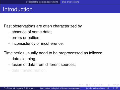
Past observations are often characterized by- absence of some data;- errors or outliers;- inconsistency or incoherence.
Time series usually need to be preprocessed as follows:- data cleaning;- fusion of data from different sources;- data transformation.
G. Ghiani, G. Laporte, R. Musmanno Introduction to Logistics System Management © John Wiley & Sons, Ltd 2 / 33
2 Forecasting logistics requirements Data preprocessing
Introduction
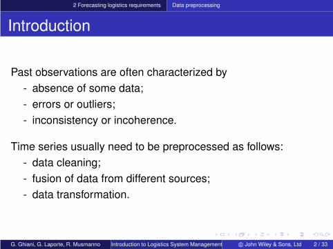
Past observations are often characterized by- absence of some data;- errors or outliers;- inconsistency or incoherence.
Time series usually need to be preprocessed as follows:- data cleaning;- fusion of data from different sources;- data transformation.
G. Ghiani, G. Laporte, R. Musmanno Introduction to Logistics System Management © John Wiley & Sons, Ltd 2 / 33

2 Forecasting logistics requirements Data preprocessing
Introduction
Past observations are often characterized by- absence of some data;- errors or outliers;- inconsistency or incoherence.
Time series usually need to be preprocessed as follows:- data cleaning;- fusion of data from different sources;- data transformation.
G. Ghiani, G. Laporte, R. Musmanno Introduction to Logistics System Management © John Wiley & Sons, Ltd 2 / 33
2 Forecasting logistics requirements Data preprocessing
Insertion of missing data (1/3)
Simplest case:
a missing observation can be replaced with the average of theprevious and subsequent observations.
G. Ghiani, G. Laporte, R. Musmanno Introduction to Logistics System Management © John Wiley & Sons, Ltd 3 / 33
2 Forecasting logistics requirements Data preprocessing
Insertion of missing data (2/3)
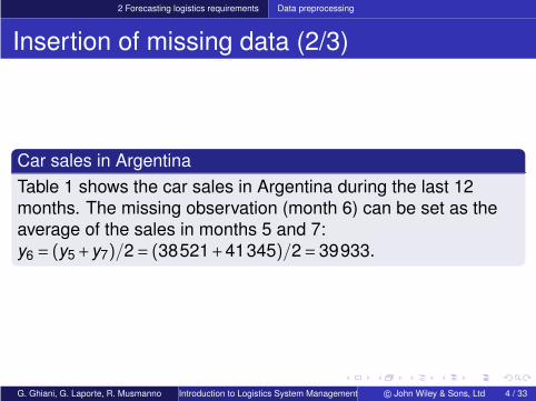
Car sales in ArgentinaTable 1 shows the car sales in Argentina during the last 12months. The missing observation (month 6) can be set as theaverage of the sales in months 5 and 7:y6 = (y5+y7)/2= (38521+41345)/2= 39933.
G. Ghiani, G. Laporte, R. Musmanno Introduction to Logistics System Management © John Wiley & Sons, Ltd 4 / 33
2 Forecasting logistics requirements Data preprocessing
Insertion of missing data (3/3)
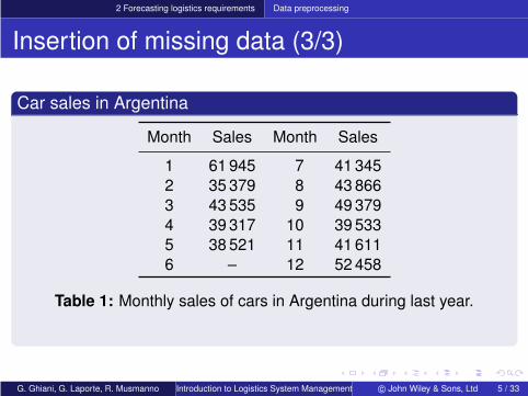
Car sales in Argentina
Month Sales Month Sales
1 61 945 7 41 3452 35 379 8 43 8663 43 535 9 49 3794 39 317 10 39 5335 38 521 11 41 6116 – 12 52 458
Table 1: Monthly sales of cars in Argentina during last year.
G. Ghiani, G. Laporte, R. Musmanno Introduction to Logistics System Management © John Wiley & Sons, Ltd 5 / 33
2 Forecasting logistics requirements Data preprocessing
Outliers
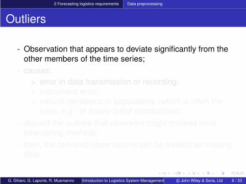
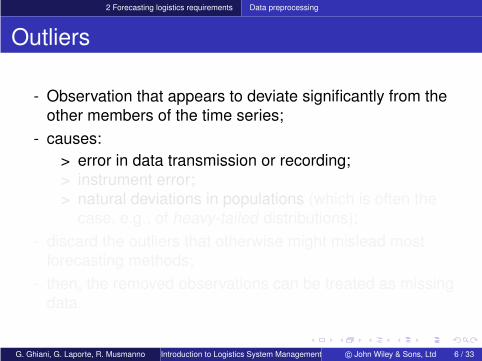
- Observation that appears to deviate significantly from theother members of the time series;
- causes:> error in data transmission or recording;> instrument error;> natural deviations in populations (which is often the
case, e.g., of heavy-tailed distributions);- discard the outliers that otherwise might mislead most
forecasting methods;- then, the removed observations can be treated as missing
data.
G. Ghiani, G. Laporte, R. Musmanno Introduction to Logistics System Management © John Wiley & Sons, Ltd 6 / 33
2 Forecasting logistics requirements Data preprocessing
Outliers
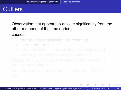
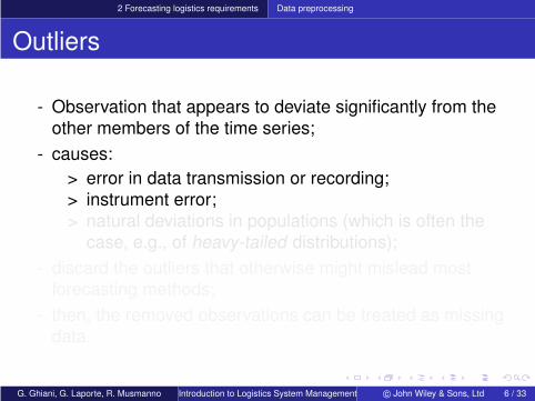
- Observation that appears to deviate significantly from theother members of the time series;
- causes:> error in data transmission or recording;> instrument error;> natural deviations in populations (which is often the
case, e.g., of heavy-tailed distributions);- discard the outliers that otherwise might mislead most
forecasting methods;- then, the removed observations can be treated as missing
data.
G. Ghiani, G. Laporte, R. Musmanno Introduction to Logistics System Management © John Wiley & Sons, Ltd 6 / 33
2 Forecasting logistics requirements Data preprocessing
Outliers
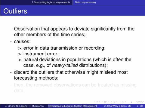
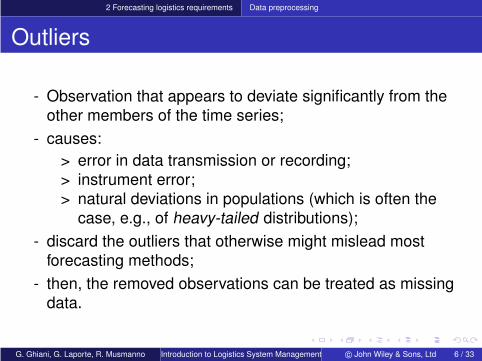
- Observation that appears to deviate significantly from theother members of the time series;
- causes:> error in data transmission or recording;> instrument error;> natural deviations in populations (which is often the
case, e.g., of heavy-tailed distributions);- discard the outliers that otherwise might mislead most
forecasting methods;- then, the removed observations can be treated as missing
data.
G. Ghiani, G. Laporte, R. Musmanno Introduction to Logistics System Management © John Wiley & Sons, Ltd 6 / 33

2 Forecasting logistics requirements Data preprocessing
Outliers
- Observation that appears to deviate significantly from theother members of the time series;
- causes:> error in data transmission or recording;> instrument error;> natural deviations in populations (which is often the
case, e.g., of heavy-tailed distributions);- discard the outliers that otherwise might mislead most
forecasting methods;- then, the removed observations can be treated as missing
data.
G. Ghiani, G. Laporte, R. Musmanno Introduction to Logistics System Management © John Wiley & Sons, Ltd 6 / 33
2 Forecasting logistics requirements Data preprocessing
Detection of outliers (1/3)
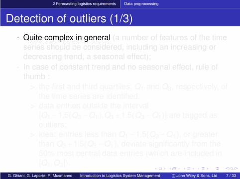
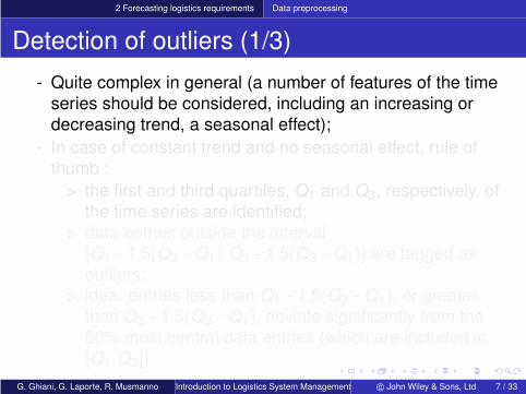
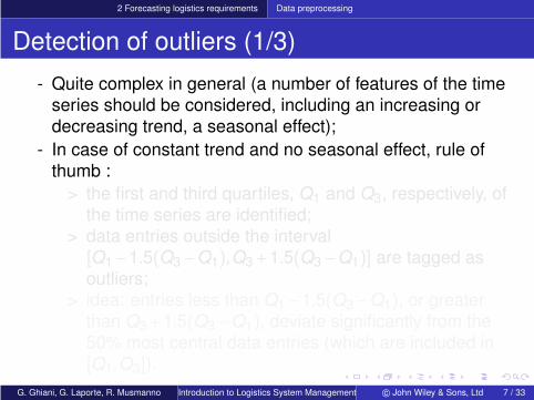
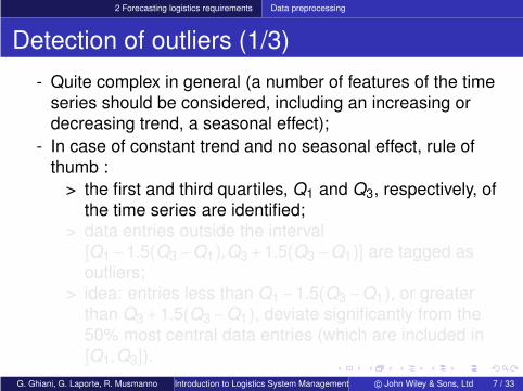
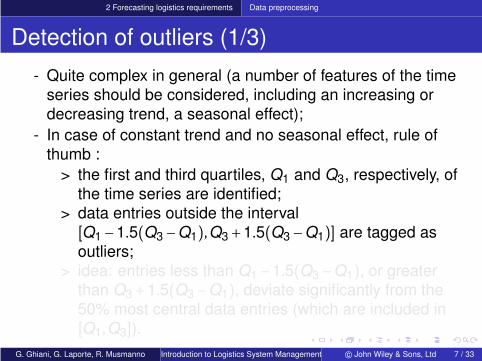
- Quite complex in general (a number of features of the timeseries should be considered, including an increasing ordecreasing trend, a seasonal effect);
- In case of constant trend and no seasonal effect, rule ofthumb :
> the first and third quartiles, Q1 and Q3, respectively, ofthe time series are identified;
> data entries outside the interval[Q1−1.5(Q3−Q1),Q3+1.5(Q3−Q1)] are tagged asoutliers;
> idea: entries less than Q1−1.5(Q3−Q1), or greaterthan Q3+1.5(Q3−Q1), deviate significantly from the50% most central data entries (which are included in[Q1,Q3]).
G. Ghiani, G. Laporte, R. Musmanno Introduction to Logistics System Management © John Wiley & Sons, Ltd 7 / 33
2 Forecasting logistics requirements Data preprocessing
Detection of outliers (1/3)
- Quite complex in general (a number of features of the timeseries should be considered, including an increasing ordecreasing trend, a seasonal effect);
- In case of constant trend and no seasonal effect, rule ofthumb :
> the first and third quartiles, Q1 and Q3, respectively, ofthe time series are identified;
> data entries outside the interval[Q1−1.5(Q3−Q1),Q3+1.5(Q3−Q1)] are tagged asoutliers;
> idea: entries less than Q1−1.5(Q3−Q1), or greaterthan Q3+1.5(Q3−Q1), deviate significantly from the50% most central data entries (which are included in[Q1,Q3]).
G. Ghiani, G. Laporte, R. Musmanno Introduction to Logistics System Management © John Wiley & Sons, Ltd 7 / 33

2 Forecasting logistics requirements Data preprocessing
Detection of outliers (2/3)
ElleshopElleshop distributes electrical appliances in Austria. Table 2reports its sales of TV sets in the province of Klagenfurt duringthe last 12 months. Since the trend is constant and there are nocyclical effects, we can apply the rule of thumb described in thissection. The first and third quartiles of the time series are,respectively, Q1 = 866.25, Q3 = 977.50. Consequently, theinterval [Q1−1.5(Q3−Q1),Q3+1.5(Q3−Q1)] is[699.375,1144.375]. This indicates that the observation relatedto month 8 is an outlier. The value y8 is therefore eliminated andreplaced by 825, the average of the sales volumes in months 7and 9.
G. Ghiani, G. Laporte, R. Musmanno Introduction to Logistics System Management © John Wiley & Sons, Ltd 8 / 33

2 Forecasting logistics requirements Data preprocessing
Detection of outliers (3/3)
Elleshop
Period Sales Period Sales
1 975 7 7702 1025 8 2003 895 9 8804 1055 10 8705 925 11 9156 985 12 855
Table 2: Number of TV sets delivered during the last 12 months byElleshop.
G. Ghiani, G. Laporte, R. Musmanno Introduction to Logistics System Management © John Wiley & Sons, Ltd 9 / 33

2 Forecasting logistics requirements Data preprocessing
Data aggregation (1/8)
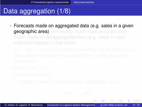
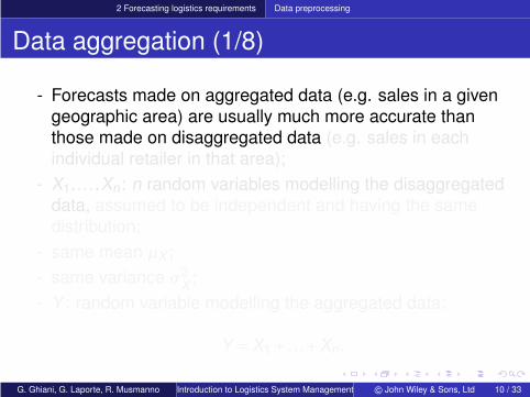
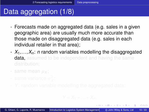
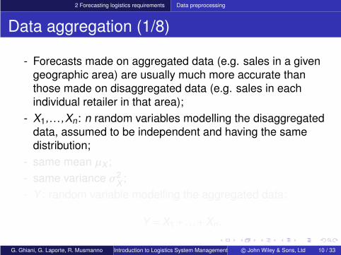
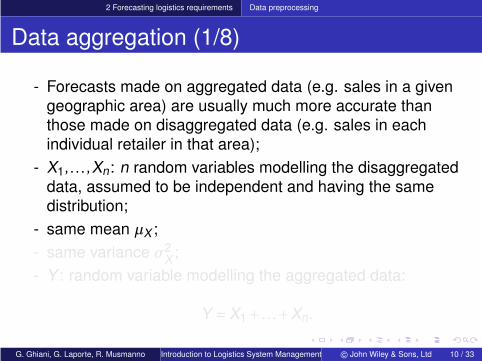
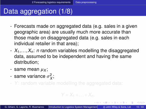
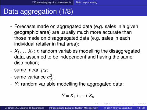
- Forecasts made on aggregated data (e.g. sales in a givengeographic area) are usually much more accurate thanthose made on disaggregated data (e.g. sales in eachindividual retailer in that area);
- X1, . . . ,Xn: n random variables modelling the disaggregateddata, assumed to be independent and having the samedistribution;
- same mean µX ;- same variance σ
2X ;
- Y : random variable modelling the aggregated data:
Y =X1+ . . .+Xn.
G. Ghiani, G. Laporte, R. Musmanno Introduction to Logistics System Management © John Wiley & Sons, Ltd 10 / 33
2 Forecasting logistics requirements Data preprocessing
Data aggregation (1/8)
- Forecasts made on aggregated data (e.g. sales in a givengeographic area) are usually much more accurate thanthose made on disaggregated data (e.g. sales in eachindividual retailer in that area);
- X1, . . . ,Xn: n random variables modelling the disaggregateddata, assumed to be independent and having the samedistribution;
- same mean µX ;- same variance σ
2X ;
- Y : random variable modelling the aggregated data:
Y =X1+ . . .+Xn.
G. Ghiani, G. Laporte, R. Musmanno Introduction to Logistics System Management © John Wiley & Sons, Ltd 10 / 33
2 Forecasting logistics requirements Data preprocessing
Data aggregation (2/8)
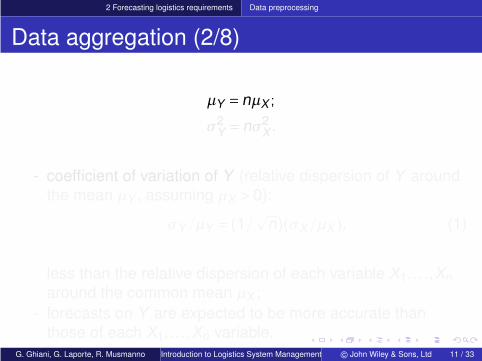
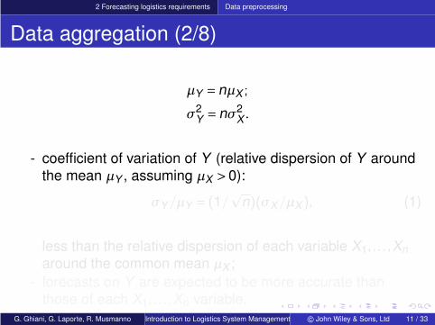
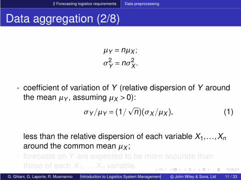
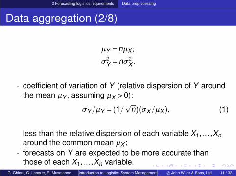
µY = nµX ;
σ2Y = nσ2
X .
- coefficient of variation of Y (relative dispersion of Y aroundthe mean µY , assuming µX > 0):
σY/µY = (1/p
n)(σX/µX ), (1)
less than the relative dispersion of each variable X1, . . . ,Xnaround the common mean µX ;
- forecasts on Y are expected to be more accurate thanthose of each X1, . . . ,Xn variable.
G. Ghiani, G. Laporte, R. Musmanno Introduction to Logistics System Management © John Wiley & Sons, Ltd 11 / 33

2 Forecasting logistics requirements Data preprocessing
Data aggregation (2/8)
µY = nµX ;
σ2Y = nσ2
X .
- coefficient of variation of Y (relative dispersion of Y aroundthe mean µY , assuming µX > 0):
σY/µY = (1/p
n)(σX/µX ), (1)
less than the relative dispersion of each variable X1, . . . ,Xnaround the common mean µX ;
- forecasts on Y are expected to be more accurate thanthose of each X1, . . . ,Xn variable.
G. Ghiani, G. Laporte, R. Musmanno Introduction to Logistics System Management © John Wiley & Sons, Ltd 11 / 33
2 Forecasting logistics requirements Data preprocessing
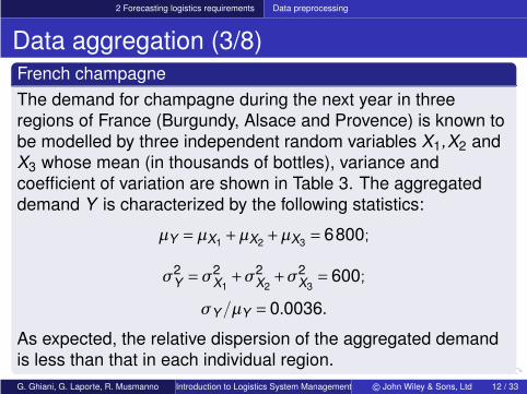
Data aggregation (3/8)French champagneThe demand for champagne during the next year in threeregions of France (Burgundy, Alsace and Provence) is known tobe modelled by three independent random variables X1,X2 andX3 whose mean (in thousands of bottles), variance andcoefficient of variation are shown in Table 3. The aggregateddemand Y is characterized by the following statistics:
µY =µX1 +µX2 +µX3 = 6800;
σ2Y =σ
2X1
+σ2X2
+σ2X3
= 600;
σY/µY = 0.0036.
As expected, the relative dispersion of the aggregated demandis less than that in each individual region.G. Ghiani, G. Laporte, R. Musmanno Introduction to Logistics System Management © John Wiley & Sons, Ltd 12 / 33
2 Forecasting logistics requirements Data preprocessing
Data aggregation (4/8)
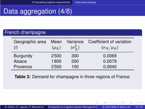
French champagne
Geographic area Mean Variance Coefficient of variation(i) (µXi ) (σ2
Xi) (σXi/µXi )
Burgundy 2500 300 0.0069Alsace 1800 200 0.0079Provence 2500 100 0.0040
Table 3: Demand for champagne in three regions of France.
G. Ghiani, G. Laporte, R. Musmanno Introduction to Logistics System Management © John Wiley & Sons, Ltd 13 / 33

2 Forecasting logistics requirements Data preprocessing
Data aggregation (5/8)
- Important when dealing with sporadic time series since thepresence of zero values in the time series could causeerrors most forecasting methods;
- available data grouped by product type, by differentgeographic areas or by time periods.
G. Ghiani, G. Laporte, R. Musmanno Introduction to Logistics System Management © John Wiley & Sons, Ltd 14 / 33

2 Forecasting logistics requirements Data preprocessing
Data aggregation (6/8)
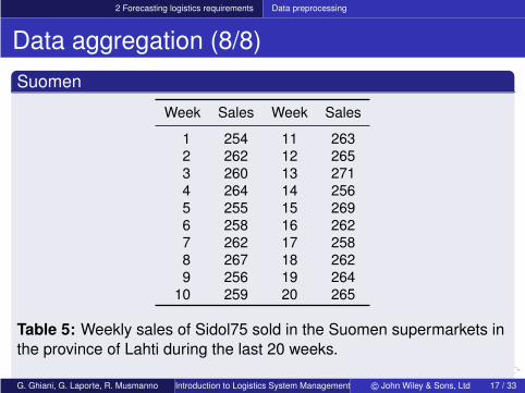
SuomenThe daily sales of Sidol75 aluminum-polishing packages in eachindividual supermarket of the Suomen chain in Lahti province,Finland, are lumpy (see e.g. the past week time series for asample supermarket shown in Table 4). In order to carry out anaccurate forecast, the sales manager decided to group the salesdata of all supermarkets in the province of Lahti and to considerweekly sales figures instead of the daily data. The resulting timeseries is shown in Table 5. Based on these data, the demand forSidol75 in the Lahti province for the following week wasestimated at 264 packages.
G. Ghiani, G. Laporte, R. Musmanno Introduction to Logistics System Management © John Wiley & Sons, Ltd 15 / 33

2 Forecasting logistics requirements Data preprocessing
Data aggregation (7/8)
Suomen
Day Sales
1 42 03 04 35 86 77 0
Table 4: Daily sales of Sidol75 in a sample Suomen supermarket inthe province of Lahti.
G. Ghiani, G. Laporte, R. Musmanno Introduction to Logistics System Management © John Wiley & Sons, Ltd 16 / 33
2 Forecasting logistics requirements Data preprocessing
Data aggregation (8/8)Suomen
Week Sales Week Sales
1 254 11 2632 262 12 2653 260 13 2714 264 14 2565 255 15 2696 258 16 2627 262 17 2588 267 18 2629 256 19 264
10 259 20 265
Table 5: Weekly sales of Sidol75 sold in the Suomen supermarkets inthe province of Lahti during the last 20 weeks.
G. Ghiani, G. Laporte, R. Musmanno Introduction to Logistics System Management © John Wiley & Sons, Ltd 17 / 33

2 Forecasting logistics requirements Data preprocessing
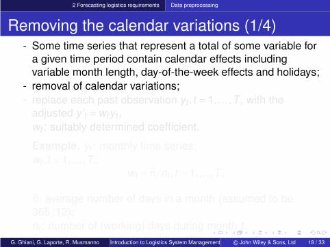
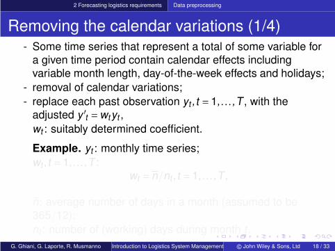
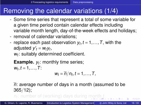
Removing the calendar variations (1/4)- Some time series that represent a total of some variable for
a given time period contain calendar effects includingvariable month length, day-of-the-week effects and holidays;
- removal of calendar variations;- replace each past observation yt , t = 1, . . . ,T , with the
adjusted y ′t =wtyt ,
wt : suitably determined coefficient.
Example. yt : monthly time series;wt , t = 1, . . . ,T :
wt = n/nt , t = 1, . . . ,T ,
n: average number of days in a month (assumed to be365/12);nt : number of (working) days during month t .
G. Ghiani, G. Laporte, R. Musmanno Introduction to Logistics System Management © John Wiley & Sons, Ltd 18 / 33
2 Forecasting logistics requirements Data preprocessing
Removing the calendar variations (1/4)- Some time series that represent a total of some variable for
a given time period contain calendar effects includingvariable month length, day-of-the-week effects and holidays;
- removal of calendar variations;- replace each past observation yt , t = 1, . . . ,T , with the
adjusted y ′t =wtyt ,
wt : suitably determined coefficient.
Example. yt : monthly time series;wt , t = 1, . . . ,T :
wt = n/nt , t = 1, . . . ,T ,
n: average number of days in a month (assumed to be365/12);nt : number of (working) days during month t .
G. Ghiani, G. Laporte, R. Musmanno Introduction to Logistics System Management © John Wiley & Sons, Ltd 18 / 33
2 Forecasting logistics requirements Data preprocessing
Removing the calendar variations (2/4)
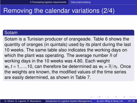
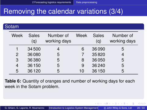
SotamSotam is a Tunisian producer of orangeade. Table 6 shows thequantity of oranges (in quintals) used by its plant during the last10 weeks. The same table also indicates the working days onwhich the plant was operating. The average number n ofworking days in the 10 weeks was 4.80. Each weightwt , t = 1, . . . ,10, can therefore be determined as wt = n/nt . Oncethe weights are known, the modified values of the time seriesare easily determined, as shown in Table 7.
G. Ghiani, G. Laporte, R. Musmanno Introduction to Logistics System Management © John Wiley & Sons, Ltd 19 / 33
2 Forecasting logistics requirements Data preprocessing
Removing the calendar variations (3/4)
Sotam
Week Sales Number of Week Sales Number of(q) working days (q) working days
1 34 500 4 6 36 090 52 36 080 5 7 35 820 43 36 380 5 8 36 050 54 36 150 5 9 36 240 55 36 120 5 10 36 150 5
Table 6: Quantity of oranges and number of working days for eachweek in the Sotam problem.
G. Ghiani, G. Laporte, R. Musmanno Introduction to Logistics System Management © John Wiley & Sons, Ltd 20 / 33

2 Forecasting logistics requirements Data preprocessing
Removing the calendar variations (4/4)
Sotam
t wt y ′t t wt y ′
t
1 1.20 41 400.00 6 0.96 34 646.402 0.96 34 636.80 7 1.20 42 984.003 0.96 34 924.80 8 0.96 34 608.004 0.96 34 704.00 9 0.96 34 790.405 0.96 34 675.20 10 0.96 34 704.00
Table 7: Modified time series of the Sotam problem obtained byremoving calendar variations.
G. Ghiani, G. Laporte, R. Musmanno Introduction to Logistics System Management © John Wiley & Sons, Ltd 21 / 33
2 Forecasting logistics requirements Data preprocessing
Deflating monetary time series (1/5)
- Inflation: significant component of apparent growth in anymonetary time series;
- monetary time series: observations measured in euros,dollars or any other currency (e.g. the sales of a finishedproduct or the prices of a raw material);
- by adjusting for inflation, real variations over time can beidentified;
- rk : average rate of inflation in time period k .
G. Ghiani, G. Laporte, R. Musmanno Introduction to Logistics System Management © John Wiley & Sons, Ltd 22 / 33
2 Forecasting logistics requirements Data preprocessing
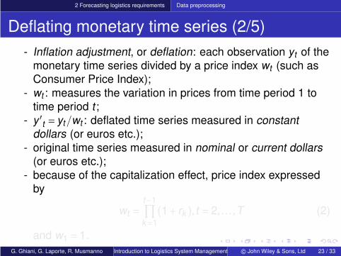
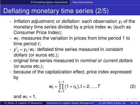
Deflating monetary time series (2/5)- Inflation adjustment, or deflation: each observation yt of the
monetary time series divided by a price index wt (such asConsumer Price Index);
- wt : measures the variation in prices from time period 1 totime period t ;
- y ′t = yt/wt : deflated time series measured in constant
dollars (or euros etc.);- original time series measured in nominal or current dollars
(or euros etc.);- because of the capitalization effect, price index expressed
by
wt =t−1∏
k=1(1+ rk ), t = 2, . . . ,T (2)
and w1 = 1.G. Ghiani, G. Laporte, R. Musmanno Introduction to Logistics System Management © John Wiley & Sons, Ltd 23 / 33

2 Forecasting logistics requirements Data preprocessing
Deflating monetary time series (2/5)- Inflation adjustment, or deflation: each observation yt of the
monetary time series divided by a price index wt (such asConsumer Price Index);
- wt : measures the variation in prices from time period 1 totime period t ;
- y ′t = yt/wt : deflated time series measured in constant
dollars (or euros etc.);- original time series measured in nominal or current dollars
(or euros etc.);- because of the capitalization effect, price index expressed
by
wt =t−1∏
k=1(1+ rk ), t = 2, . . . ,T (2)
and w1 = 1.G. Ghiani, G. Laporte, R. Musmanno Introduction to Logistics System Management © John Wiley & Sons, Ltd 23 / 33

2 Forecasting logistics requirements Data preprocessing
Deflating monetary time series (3/5)
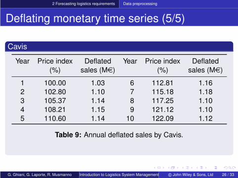
CavisCavis is a wine-making company that sells its products almostexclusively in France. The annual sales during the last 10 yearsare reported in Table 8. The same table also shows the annualrate of inflation recorded in the time period. The deflated data,obtained through (2), are reported in Table 9.
G. Ghiani, G. Laporte, R. Musmanno Introduction to Logistics System Management © John Wiley & Sons, Ltd 24 / 33

2 Forecasting logistics requirements Data preprocessing
Deflating monetary time series (4/5)
Cavis
Year Inflation Sales Year Inflation Salesrate (%) (Me) rate (%) (Me)
1 2.80 1.03 6 2.10 1.312 2.50 1.13 7 1.80 1.363 2.70 1.20 8 3.30 1.294 2.20 1.24 9 0.80 1.335 2.00 1.26 10 1.50 1.37
Table 8: Annual Cavis sales and the corresponding annual inflationrates.
G. Ghiani, G. Laporte, R. Musmanno Introduction to Logistics System Management © John Wiley & Sons, Ltd 25 / 33
2 Forecasting logistics requirements Data preprocessing
Deflating monetary time series (5/5)
Cavis
Year Price index Deflated Year Price index Deflated(%) sales (Me) (%) sales (Me)
1 100.00 1.03 6 112.81 1.162 102.80 1.10 7 115.18 1.183 105.37 1.14 8 117.25 1.104 108.21 1.15 9 121.12 1.105 110.60 1.14 10 122.09 1.12
Table 9: Annual deflated sales by Cavis.
G. Ghiani, G. Laporte, R. Musmanno Introduction to Logistics System Management © John Wiley & Sons, Ltd 26 / 33
2 Forecasting logistics requirements Data preprocessing
Adjusting for population variations (1/4)
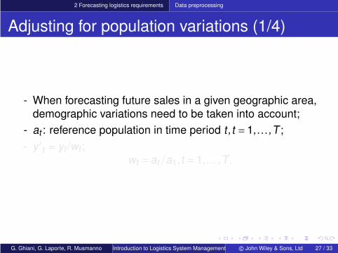
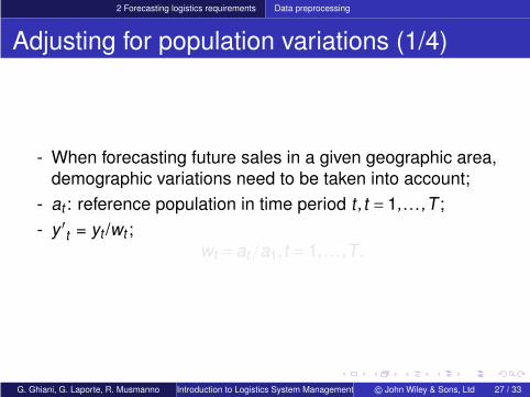
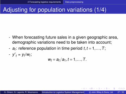
- When forecasting future sales in a given geographic area,demographic variations need to be taken into account;
- at : reference population in time period t , t = 1, . . . ,T ;- y ′
t = yt /wt ;wt = at/a1, t = 1, . . . ,T .
G. Ghiani, G. Laporte, R. Musmanno Introduction to Logistics System Management © John Wiley & Sons, Ltd 27 / 33
2 Forecasting logistics requirements Data preprocessing
Adjusting for population variations (1/4)
- When forecasting future sales in a given geographic area,demographic variations need to be taken into account;
- at : reference population in time period t , t = 1, . . . ,T ;- y ′
t = yt /wt ;wt = at/a1, t = 1, . . . ,T .
G. Ghiani, G. Laporte, R. Musmanno Introduction to Logistics System Management © John Wiley & Sons, Ltd 27 / 33
2 Forecasting logistics requirements Data preprocessing
Adjusting for population variations (2/4)
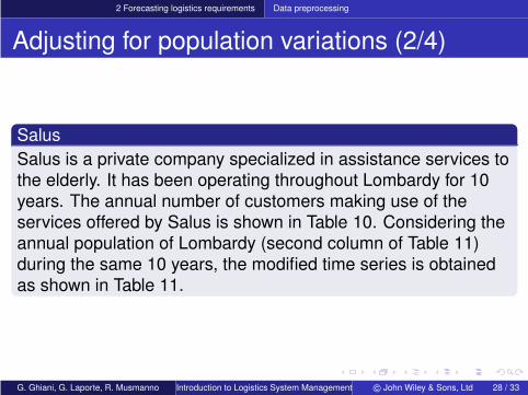
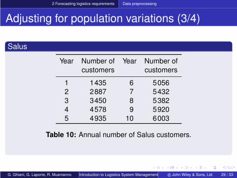
SalusSalus is a private company specialized in assistance services tothe elderly. It has been operating throughout Lombardy for 10years. The annual number of customers making use of theservices offered by Salus is shown in Table 10. Considering theannual population of Lombardy (second column of Table 11)during the same 10 years, the modified time series is obtainedas shown in Table 11.
G. Ghiani, G. Laporte, R. Musmanno Introduction to Logistics System Management © John Wiley & Sons, Ltd 28 / 33
2 Forecasting logistics requirements Data preprocessing
Adjusting for population variations (3/4)
Salus
Year Number of Year Number ofcustomers customers
1 1435 6 50562 2887 7 54323 3450 8 53824 4578 9 59205 4935 10 6003
Table 10: Annual number of Salus customers.
G. Ghiani, G. Laporte, R. Musmanno Introduction to Logistics System Management © John Wiley & Sons, Ltd 29 / 33
2 Forecasting logistics requirements Data preprocessing
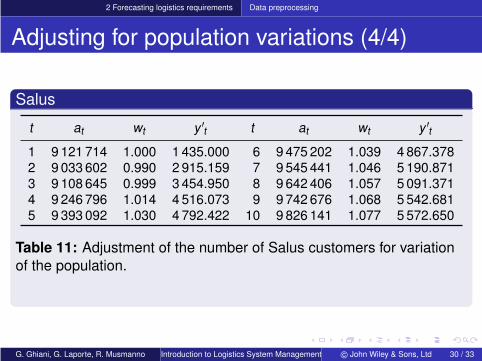
Adjusting for population variations (4/4)
Salus
t at wt y ′t t at wt y ′
t
1 9 121 714 1.000 1 435.000 6 9 475 202 1.039 4 867.3782 9 033 602 0.990 2 915.159 7 9 545 441 1.046 5 190.8713 9 108 645 0.999 3 454.950 8 9 642 406 1.057 5 091.3714 9 246 796 1.014 4 516.073 9 9 742 676 1.068 5 542.6815 9 393 092 1.030 4 792.422 10 9 826 141 1.077 5 572.650
Table 11: Adjustment of the number of Salus customers for variationof the population.
G. Ghiani, G. Laporte, R. Musmanno Introduction to Logistics System Management © John Wiley & Sons, Ltd 30 / 33
2 Forecasting logistics requirements Data preprocessing
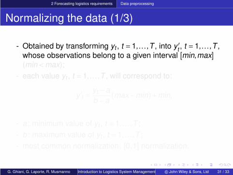
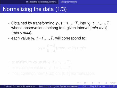
Normalizing the data (1/3)
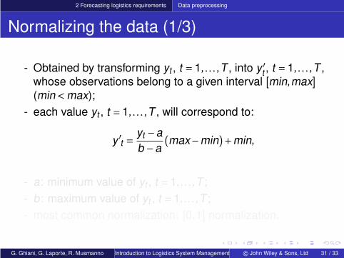
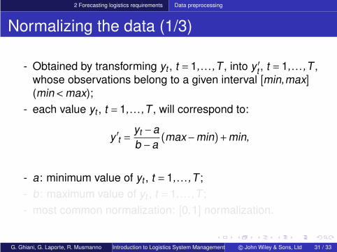
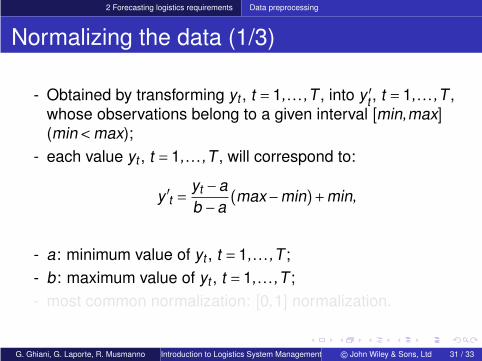
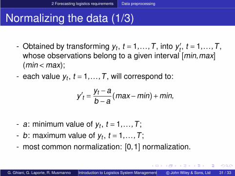
- Obtained by transforming yt , t = 1, . . . ,T , into y ′t , t = 1, . . . ,T ,
whose observations belong to a given interval [min,max](min<max);
- each value yt , t = 1, . . . ,T , will correspond to:
y ′t =
yt −ab −a
(max−min)+min,
- a: minimum value of yt , t = 1, . . . ,T ;- b: maximum value of yt , t = 1, . . . ,T ;- most common normalization: [0,1] normalization.
G. Ghiani, G. Laporte, R. Musmanno Introduction to Logistics System Management © John Wiley & Sons, Ltd 31 / 33

2 Forecasting logistics requirements Data preprocessing
Normalizing the data (1/3)
- Obtained by transforming yt , t = 1, . . . ,T , into y ′t , t = 1, . . . ,T ,
whose observations belong to a given interval [min,max](min<max);
- each value yt , t = 1, . . . ,T , will correspond to:
y ′t =
yt −ab −a
(max−min)+min,
- a: minimum value of yt , t = 1, . . . ,T ;- b: maximum value of yt , t = 1, . . . ,T ;- most common normalization: [0,1] normalization.
G. Ghiani, G. Laporte, R. Musmanno Introduction to Logistics System Management © John Wiley & Sons, Ltd 31 / 33

2 Forecasting logistics requirements Data preprocessing
Normalizing the data (2/3)
ExampleThe time series of Sotam shown in Table 7 (third and sixthcolumns), when normalized in the interval [2000,4000], willresult in Table 12.
G. Ghiani, G. Laporte, R. Musmanno Introduction to Logistics System Management © John Wiley & Sons, Ltd 32 / 33

2 Forecasting logistics requirements Data preprocessing
Normalizing the data (3/3)
Example
t y ′t t y ′
t
1 3 621.78 6 2 009.172 2 006.88 7 4 000.003 2 075.64 8 2 000.004 2 022.92 9 2 043.555 2 016.05 10 2 022.92
Table 12: Sotam time series normalized in interval [2000,4000].
G. Ghiani, G. Laporte, R. Musmanno Introduction to Logistics System Management © John Wiley & Sons, Ltd 33 / 33