2-D tomography of volcanic CO from scanning hard target ...€¦ · 2-D tomography of volcanic CO 2 from scanning hard target differential absorption LIDAR: The case of Solfatara,

The University of Manchester Research

2-D tomography of volcanic CO2 from scanning hard targetdifferential absorption LIDARDOI:10.5194/amt-2016-166

Document VersionFinal published version

Link to publication record in Manchester Research Explorer

Citation for published version (APA):Queisser, M., Granieri, D., & Burton, M. (2016). 2-D tomography of volcanic CO2 from scanning hard targetdifferential absorption LIDAR: The case of Solfatara, Campi Flegrei. Atmospheric Measurement Techniques.https://doi.org/10.5194/amt-2016-166

Published in:Atmospheric Measurement Techniques

Citing this paperPlease note that where the full-text provided on Manchester Research Explorer is the Author Accepted Manuscriptor Proof version this may differ from the final Published version. If citing, it is advised that you check and use thepublisher's definitive version.

General rightsCopyright and moral rights for the publications made accessible in the Research Explorer are retained by theauthors and/or other copyright owners and it is a condition of accessing publications that users recognise andabide by the legal requirements associated with these rights.

Takedown policyIf you believe that this document breaches copyright please refer to the University of Manchester’s TakedownProcedures [http://man.ac.uk/04Y6Bo] or contact [email protected] providingrelevant details, so we can investigate your claim.

Download date:15. Jun. 2020

https://doi.org/10.5194/amt-2016-166

https://www.research.manchester.ac.uk/portal/en/publications/2d-tomography-of-volcanic-co2-from-scanning-hard-target-differential-absorption-lidar(475c5668-3552-4bc0-a3f9-36c9b54442a8).html

/portal/mike.burton.html



https://doi.org/10.5194/amt-2016-166

1

2-D tomography of volcanic CO2 from scanning hard target

differential absorption LIDAR: The case of Solfatara, Campi Flegrei

(Italy)

Manuel Queiβer1, Domenico Granieri2, Mike Burton1

1School of Earth, Atmospheric and Environmental Sciences, University of Manchester, Oxford Road, Manchester M13 9PL, 5

UK 2Istituto Nazionale di Geofisica e Vulcanologia (INGV), Sezione di Pisa, 50126 Pisa, Italy

Correspondence to: Manuel Queiβer ([email protected]), Tel.: +44(0)161 2750778, Fax.: +44(0)161 306

9361

10

Abstract. Solfatara is part of the active volcanic zone of Campi Flegrei (Italy), a densely populated urban area where ground

uplift and increasing ground temperature are observed, connected with rising rates of CO2 emission. A major pathway of CO2

release at Campi Flegrei is diffuse soil degassing, and therefore quantifying diffuse CO2 emission rates is of vital interest.

Conventional in-situ probing of soil gas emissions with accumulation chambers is accurate over a small footprint but requires

significant time and effort to cover large areas. An alternative approach is differential absorption LIDAR, which allows for a 15

fast and spatially integrated measurement. Here, a portable hard-target differential absorption LIDAR has been used to acquire

horizontal 1-D profiles of CO2 concentration at the Solfatara crater. To capture the non-isotropic nature of the diffuse degassing

activity, a 2-D tomographic map of the CO2 distribution has been inverted from the 1-D profiles. The acquisition was performed

from a single half space only, which increases the non-linearity of the inverse problem. Nonetheless, the result is in agreement

with independent measurements and furthermore confirms an area of anomalous CO2 degassing along the eastern edge as well 20

as the center of the Solfatara crater. The method has important implications for measurements of degassing features that can

only be accessed from limited angles, such as airborne sensing of volcanic plumes. CO2 fluxes retrieved from the 2-D map are

comparable, but modestly higher than emission rates from previous studies, perhaps reflecting a more integrated measurement.

1 Introduction 25

Subaerial volcanoes emit a variety of gaseous species, dominated by water vapor and CO2, and aerosols. Originating from

exsolution processes that may take place deep in the crust due to the low solubility of CO2 in magmas, volcanic CO2 is a

powerful tracer for magmatic recharge and ascent processes (Burton et al., 2013; Frezzotti et al., 2014; Chiodini et al., 2015;

La Spina et al., 2015). Measuring volcanic CO2 emission rates is therefore also a feasible pathway towards improved

forecasting of volcanic activity, such as seismicity or eruptions (Petrazzuoli et al., 1999; Carapezza et al. 2004; Aiuppa et al., 30

Atmos. Meas. Tech. Discuss., doi:10.5194/amt-2016-166, 2016Manuscript under review for journal Atmos. Meas. Tech.Published: 8 August 2016c© Author(s) 2016. CC-BY 3.0 License.

2

2011). Unfortunately, magmatic CO2 is not only released actively via vents such as the volcano mouth, but also diffusively via

soil or flank degassing (Baubron et al., 1991; Hards, 2005; Chiodini et al., 2007). In addition, in most cases the volcanic CO2

signal is modest compared with ambient concentrations (Burton et al., 2013) and quickly diluted into the atmosphere. A

common approach to determine the magmatic CO2 flux is based on a gridded sampling of the CO2 distribution in the volcanic

plume itself (Gerlach et al., 1997; Lewicki et al., 2005; Diaz et al., 2010; Lee et al., 2016) from which 2-D CO2 concentration 5

maps are retrieved by secondary data processing, such as statistical methods (Lewicki et al., 2005; McGee et al., 2008) and

dispersion modeling (Aiuppa et al., 2013; Granieri et al., 2014). Integrating the CO2 concentrations over the cross sectional

plume area and multiplying the result with the transport speed perpendicular to the cross section yields CO2 fluxes. The in situ

method has two drawbacks. Firstly, it may be dangerous to perform in situ measurements from within the volcanic plume (e.g.

due to toxic gases or low visibility near the crater mouth). Secondly, in situ methods allow for a very accurate estimation of 10

CO2 concentration, but only in the vicinity of the measurement point, potentially missing significant contributions from in

between the measurement points.

Remote sensing techniques (see Platt et al., 2015 for overview of state-of-the-art), notably active remote sensing

platforms, including differential absorption LIDAR (DIAL) and spectrometers (Menzies and Chahine, 1974; Weibring et al.,

1998; Koch et al., 2004; Kameyama et al., 2009) acquire columns of range resolved (Sakaizawa et al., 2009; Aiuppa et al., 15

2015) or column averaged (Amediek et al., 2008; Kameyama et al., 2009) CO2 concentrations. They provide a powerful tool

to overcome the aforementioned drawbacks of in situ measurement techniques by offering a faster, safer and comprehensive

acquisition (spatial coverage yields inclusive CO2 concentration profiles). Moreover, there is no need for receivers or

retroreflectors at the opposite end of the measurement column, which increases not only flexibility and timeliness of the

acquisition, but is crucial for some measurements, including airborne or spaceborne acquisitions. 20

Active remote sensing platforms based on hard target DIAL (topographic target DIAL) can use continuous wave

lasers. This allows for high signal return and compact, rugged and portable instruments, which is desirable for platform

independent measurement of atmospheric CO2, be it ground based or air-borne (Sakaizawa et al., 2013; Queißer et al., 2015a).

Yet, the drawback compared with “traditional”, pulsed DIAL is that no range resolved CO2 concentrations are measured, but

column densities (in m-2) or, as in this work, path length concentration products (called “path amount” hereafter, in ppm.m). 25

By scanning across the emission feature one obtains 1-D profiles of path amounts. Using these profiles to determine CO2

fluxes is straightforward only for gas plumes for which a homogeneous cross section can be assumed (Galle et al., 2010).

However, particularly diffuse degassing activities are often not associated with homogeneous, but an unknown CO2

distribution within the scanned plume cross section. Therefore, the assumption of homogenous CO2 distribution may lead to

under or overestimated CO2 fluxes when probed from different directions, since path amounts are measured, which represent 30

path averaged CO2 concentrations. It would be very desirable, and this was the main motivation of this work, to have a 2-D

map that at least contains the geometry of the anomalous CO2 release, let aside precise CO2 mixing ratios. This would allow

to geometrically correct the fluxes derived from CO2 path amounts delivered by hard target DIAL systems. Provided the 2-D

map contains correct CO2 mixing ratios, the CO2 flux can be conveniently obtained by simple integration over the 2-D map.


3

Note that tomographic reconstructions of volcanic gas plumes have already been performed, however, for SO2 and using

passive remote sensing techniques (Kazahaya et al., 2008; Wright et al., 2008; Johansson et al., 2009).

The study was focusing on a zone of diffuse degassing of magmatic CO2 within the Solfatara crater (Italy) reported

previously (e.g. Bagnato et al., 2014). Solfatara is a fumarolic field and part of the active volcanic area of Campi Flegrei (CF,

Fig. 1). CF is a nested caldera, resulting from two large collapses, the last one ~15 ka ago (Scarpati et al., 1993). CF is in direct 5

vicinity to the metropolis of Naples and thus a direct threat to millions of residents. Thanks to its accessibility and strong CO2

degassing Solfatara provides almost a model like volcano, a natural laboratory, to test new sensing approaches. On the other

hand, it is part of one of the most dangerous volcanic zones in the world, showing ground uplift coupled with seismic activity

with magma degassing likely having a significant role in triggering unrest (Chiodini at al., 2010). Solfatara therefore merits

particular monitoring efforts and any new results on observables, may they stem from well-tried or new methods, are of direct 10

importance to understand the fate of this active volcanic system.

2 Methods

2.1 Measuring 1-D profiles of CO2 path amounts

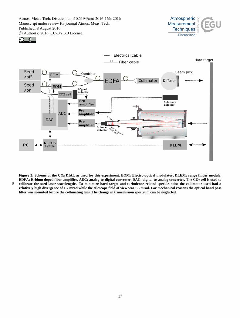
The CO2DIAL (Fig. 2) is an active remote sensing platform based on the differential absorption LIDAR principle (Koch et al.,

2004; Amediek et al., 2008). It is a further development of the portable instrument described in Queißer et al. (2015a, 2015b). 15

By taking the ratio of the optical powers associated with the received signals for the wavelengths coinciding with an absorption

line of CO2 and the wavelength at the line edge, and , respectively, one arrives at

2 ∫ 𝑑𝑟∆𝜎(𝑟)𝑁𝐶𝑂2(𝑟)

𝑅

0= − ln (

𝑃(𝜆𝑂𝑁)𝑃(𝜆𝑂𝐹𝐹)𝑟𝑒𝑓

𝑃(𝜆𝑂𝐹𝐹)𝑃(𝜆𝑂𝑁)𝑟𝑒𝑓), (1)

≡ ∆𝜏

where 𝑁𝐶𝑂2 is the CO2 number density, 𝑅 is the range, i.e. the distance between the instrument and the hard target, ∆𝜎 is the 20

difference between the molecular absorption cross sections of CO2 associated with 𝜆𝑂𝑁 and 𝜆𝑂𝐹𝐹 , 𝑃(𝜆) is the received

(“science”) and 𝑃(𝜆) 𝑟𝑒𝑓 the transmitted optical power (“reference”). The latter is measured as a reference to normalize

fluctuations of the transmitted power. The normalized optical power in Eq. (1) is referred to as grand ratio (GR),

𝐺𝑅 =𝑃(𝜆𝑂𝑁)𝑃(𝜆𝑂𝐹𝐹)𝑟𝑒𝑓

𝑃(𝜆𝑂𝐹𝐹)𝑃(𝜆𝑂𝑁)𝑟𝑒𝑓 (2)

∆𝜏 is the differential optical depth. The two distributed feedback (DFB) fiber seed lasers emit at 𝜆𝑂𝑁=1572.992 nm and 𝜆𝑂𝐹𝐹= 25

1573.173 nm (Rothman et al., 2013). To be able to easily reject background noise (such as solar background) lock-in detection

is used. Consequently, both seed laser beams (for 𝜆𝑂𝑁 and 𝜆𝑂𝐹𝐹) are amplitude modulated using two LiNbO3 electro-optical

modulators (EOM) at slightly different sine tones near 5 kHz and simultaneously amplified by an Erbium doped fiber amplifier

(EDFA) before being transmitted. The transmitted optical power can be adjusted between ~80 mW and a maximum of 1.5 W.

A glass wedge scatters a fraction of the transmitted light into an integrating sphere where the reference detector is mounted. 30

ON OFF


4

The transmitted light is diffusively backscattered by a hard target, which can be any surface located up to ~2000 m away from

the instrument, and is received by a 200 mm diameter Schmidt-Cassegrain Telescope with a focal length of 1950 mm. Typically

the received optical power is a couple of nW at a bandwidth integrated noise of ~1 pW (root mean squared noise equivalent

power). The analog to digital converter (ADC) operates at 250 kSamples s-1 and has a resolution of 16-bit. The integration

time per scan angle was set to 4000 EOM modulation periods, which corresponds to data chunks of length 784 ms (integration 5

time) for both science and reference channel. Each of these four chunks of data is demodulated using a digital lock-in routine

following Dobler et al. (2013). After the lock-in operation one arrives at four DC signals, associated with the optical powers

𝑃(𝜆𝑂𝑁), 𝑃(𝜆𝑂𝐹𝐹), 𝑃(𝜆𝑂𝑁)𝑟𝑒𝑓 and 𝑃(𝜆𝑂𝐹𝐹)𝑟𝑒𝑓. ∆𝜏 is calculated using the right hand side of Eq. (1), after taking the mean of

each of the four signals. To account for the instrumental offset of ∆𝜏, prior to scanning the volcanic plume, values of ∆𝜏 were

acquired for different 𝑅 in the ambient atmosphere. The points were used to fit a calibration curve. The ordinate at R=0 gave 10

the instrumental offset. The calibration curve was also used to convert the measured in-plume ∆𝜏 to CO2 path amounts 𝑋𝐶𝑂2

𝑐𝑜𝑙

(in ppm.m). Column averaged CO2 mixing ratios 𝑋𝐶𝑂2 ,𝑎𝑣 (in ppm) were obtained by dividing path amounts by 𝑅. The range

was measured by an onboard range finder (DLEM, Jenoptik, Germany), based on a 1550 nm LIDAR with pulse energy of 500

µJ and accuracy <1 m. By pivoting the receiver/transmitter unit using a step motor values for 𝑋𝐶𝑂2

𝑐𝑜𝑙 (or 𝑋𝐶𝑂2,𝑎𝑣) per heading

were attained, and hence 1-D profiles. 15

The precision of the column averaged CO2 mixing ratio was evaluated as

(∆ 𝑋𝐶𝑂2,𝑎𝑣

𝑋𝐶𝑂2,𝑎𝑣)

2

= SNR−2 + (𝜎𝑅

⟨𝑅⟩)

2

+ 𝛿𝑆𝑝𝑒𝑐𝑘𝑙𝑒2, (3)

with the signal-to-noise-ratio (SNR)

𝑆𝑁𝑅 = [𝜎𝐺𝑅

⟨𝐺𝑅⟩

1

ln (⟨𝐺𝑅⟩)]

−1

, (4)

where ⟨𝐺𝑅⟩ and 𝜎𝐺𝑅 are the mean and standard deviation of the grand ratio, respectively. They were estimated from time series 20

acquired at fixed angles in between the scans at CF. The SNR accounts for all noise sources occurring during acquisition,

including instrumental noise, non-stationary baseline drift, solar background noise, atmospheric noise (mostly air turbulence)

and perturbation by aerosol scattering (e.g. condensed water vapor). The second term depicts the relative range uncertainty

(standard deviation of ranges 𝜎𝑅 over mean of ranges ⟨𝑅⟩) which is typically ~1 m. The relative uncertainty due to hard target

speckle was estimated as (MacKerrow et al., 1997) 25

𝛿𝑆𝑝𝑒𝑐𝑘𝑙𝑒 =1.22𝜆𝑂𝐹𝐹𝑅

𝐷𝜉, (5)

where 𝐷 is the spot diameter on the hard target (in m) and 𝜉 is the dimension of the telescope field of view (in m) on the hard

target.


5

2.2 Reconstructing a 2-D CO2 concentration map

Ranges and their respective heading angles (i.e. range vectors, referred to as rays in the following) from the scans were

converted to absolute Cartesian coordinates (𝑥, 𝑦). The goal is to obtain CO2 mixing ratios (𝑋𝐶𝑂2, in ppm) at a given point

(𝑥, 𝑦). Due to the finite spatial resolution of every measurement system this will always be an average mixing ratio within a

confined space, in this case a 2-D grid cell. The region of interest (area bounding the scans) was divided into grid cells with 5

length ∆𝑥 (in 𝑥 direction) and ∆𝑦 (in 𝑦 direction). 𝑋𝐶𝑂2 were inferred from the measured 𝑋𝐶𝑂2

𝑐𝑜𝑙

using an inverse technique

following Pedone et al. (2014). Thereby one uses the fact that the CO2 path amount is associated with the product of a range

segment and a uniform CO2 mixing ratio 𝑋𝐶𝑂2 along that range segment. For a given ray and for 𝑛 grid cells traversed by the

ray this can be written as

∑ 𝑟𝑖𝑋𝐶𝑂2,𝑖𝑛𝑖=1 = 𝑋𝐶𝑂2

𝑐𝑜𝑙 , (6) 10

where 𝑟𝑖 depicts the length of the ray segment in grid cell 𝑖 (∑ 𝑟𝑖𝑛𝑖=1 = 𝑅). 𝑋𝐶𝑂2,𝑖 is the (unknown) CO2 mixing ratio within grid

cell 𝑖 (in ppm). Including all rays, one arrives at a system of linear equations, which can be written as

𝐿𝑐 = 𝑎, (7)

where 𝐿 is a 𝑚 × 𝑛 matrix, called geometry matrix, containing all 𝑚 rays for all 𝑛 grid cells, 𝑐 is a 𝑛 × 1 matrix containing

the uniform 𝑋𝐶𝑂2 per grid cell and is the desired quantity to be inverted. 𝑎 is a 𝑚 × 1 matrix containing the measured 15

(observed) 𝑋𝐶𝑂2

𝑐𝑜𝑙 for each ray. For simplicity, 𝑛𝑥 = 𝑛𝑦 , where 𝑛𝑥, 𝑛𝑦 are the number of grid cells in 𝑥- and 𝑦-direction,

respectively. Thus, 𝑛 = 𝑛𝑥2.

To invert Eq. (7) for 𝑐 a least square solver, the MATLAB LSQR routine, was used. The algorithm iteratively seeks

values for 𝑐, which minimize the misfit ‖𝑎 − 𝐿𝑐‖. Therefore, 𝑐 represents a model with a maximized likelihood of explaining

the observed data 𝑎. By reshaping 𝑐 into the measurement 2-D grid a 2-D map was obtained. 20

2.3 CO2 flux retrieval

From the inverted 2-D map of 𝑋𝐶𝑂2 the CO2 flux was computed as

𝜙𝐶𝑂2= 10−6 𝑢𝑁𝑎𝑖𝑟

𝑀𝐶𝑂2

𝑁𝐴∬ 𝑑𝑥𝑑𝑦 𝑋𝐶𝑂2,𝑝𝑙(𝑥, 𝑦)

𝑝𝑙𝑢𝑚𝑒 (8)

where 𝑋𝐶𝑂2,𝑝𝑙 are the inverted, background corrected CO2 mixing ratios computed as 25

𝑋𝐶𝑂2,𝑝𝑙(𝑥, 𝑦) = 𝑋𝐶𝑂2(𝑥, 𝑦) − 𝑋𝐶𝑂2,𝑏𝑔, (9)

where 𝑋𝐶𝑂2,𝑏𝑔 = 380 ppm is the background CO2 mixing ratio at Solfatara measured in situ. 𝑢 is the magnitude of the

component of the plume transport speed perpendicular to the scanned cross section (in m s-1), 𝑁𝑎𝑖𝑟 is the number density of air

(in m-3), computed using meteorological data (pressure, temperature, humidity) acquired by a portable meteorological station

close to the instrument. 𝑀𝐶𝑂2 is the molar mass of CO2 (in kg mol-1) and 𝑁𝐴 is Avogadro’s constant (in mol-1). 30


6

The plume transport speed was evaluated from digital video footage acquired during the measurement, employing a

video analysis program (Tracker from Open Source Physics). Condensed water vapor aerosol emitted by various vents in the

region of interest was assumed to propagate with the same velocity as the volcanic CO2. At a given video frame a pixel was

fixed and the calibrated propagated distance (in pixels) was measured as the video proceeded. Since the frame rate of the video

was known (30 frames per second), the speed by which the tracked point and hence a parcel of gas was transported could be 5

estimated.

The relative error of the CO2 flux was estimated as

(∆𝜙𝐶𝑂2

𝜙𝐶𝑂2

)2

= (∆𝑢

𝑢)

2

+ (∬ 𝑑𝑥𝑑𝑦 ∆𝑋𝐶𝑂2,𝑝𝑙(𝑥,𝑦)𝑝𝑙𝑢𝑚𝑒

∬ 𝑑𝑥𝑑𝑦 𝑋𝐶𝑂2,𝑝𝑙(𝑥,𝑦)𝑝𝑙𝑢𝑚𝑒

)

2

,

(10)

where ∆𝑋𝐶𝑂2 ,𝑝𝑙 is the absolute error of the CO2 mixing ratio at a given point within the integrated area and ∆𝑢 is the absolute

uncertainty of the plume speed. 10

3 Results

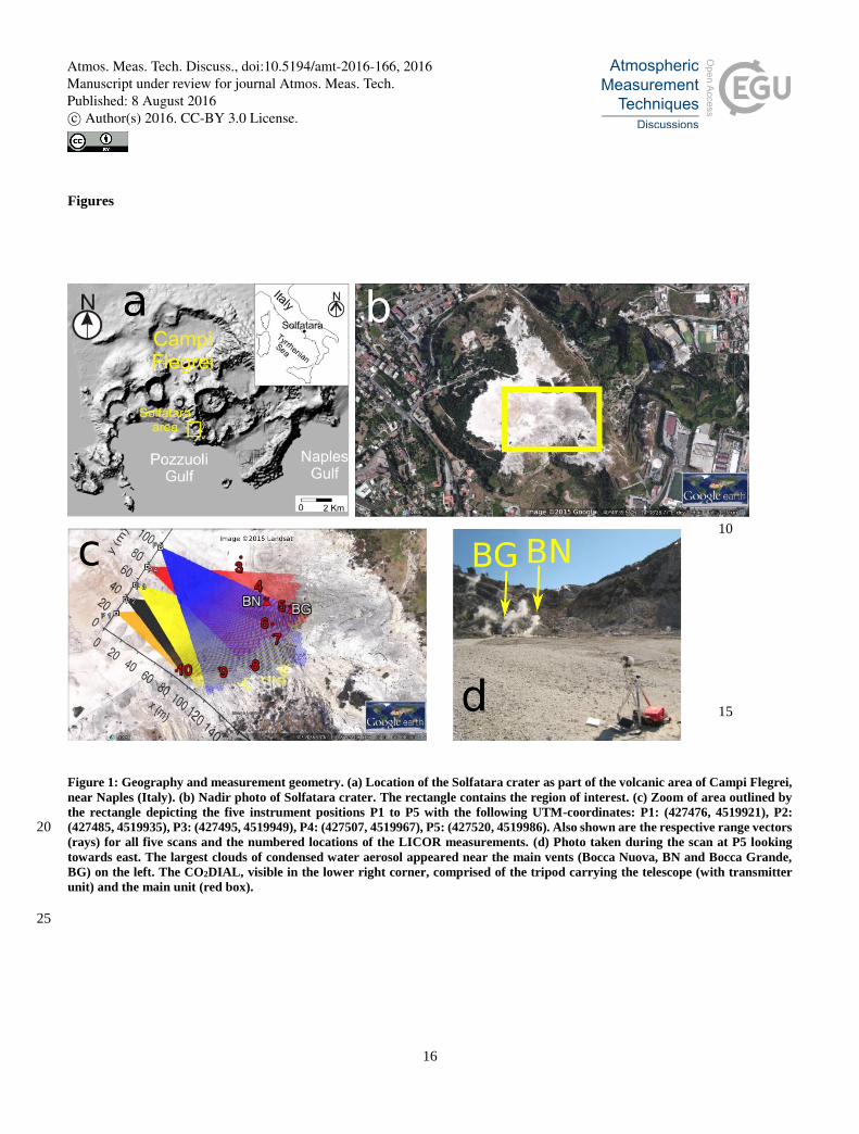
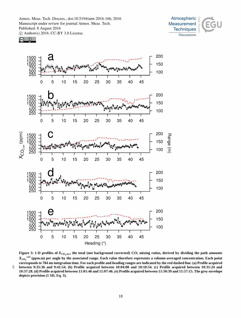
The experiment took place on 4 March 2016 inside the crater of Solfatara (Fig. 1) and was focusing on the diffuse CO2 release

alongside the Solfatara crater edge, located south of the main vents Bocca Nuova (BN) and Bocca Grande (BG), although they

were included in the scans. Elevated CO2 mixing ratios, up to 1500 ppm at places, could be affirmed by means of in situ 15

measurements using a LICOR CO2 analyzer with 4% accuracy. The LICOR analyzer was measuring at the same height as the

propagation height of the laser beam (ca. 2 m above ground). Due to logistical constraints the in situ measurements could only

be measured the day before the experiment. Five scans were performed between 9:35 and 11:57 LT (duration 142 min) from

five different locations with a total of 𝑚 = 627 beam paths (rays), which are shown along with the respective five instrument

locations in Fig 1c. It is assumed that during the complete acquisition the CO2 distribution did not change (“frozen plume”). 20

For each scan and for each heading differential optical depths ∆𝜏 have been retrieved and converted into 𝑋𝐶𝑂2

𝑐𝑜𝑙 (and 𝑋𝐶𝑂2,𝑎𝑣),

as detailed in the method section. The resulting 1-D concentration profiles are shown in Fig. 3. Numerous wiggles indicate

vigorous degassing activity, suggesting diffuse degassing or CO2 advected by local wind eddies. In addition, there are

symmetric features, such as around 26° in Fig. 3a, which appeared in scans carried out prior to the experiment and the day

before, thus suggesting vented degassing activity. The angular scanning velocity was 2.1 mrad s-1, associated with an angular 25

resolution of 1.65 mrad, which corresponds to a lateral resolution of around 24 cm between points in Fig. 3.

To invert for 𝑋𝐶𝑂2, ranges and headings were converted to Cartesian coordinates. The coordinate system was chosen

such that the instrument positions of all five scans were located on the y-axis (Fig. 1c). It proved to be useful to plot the

measured data, i.e. 𝑋𝐶𝑂2,𝑎𝑣 against their associated coordinates. The result (Fig. 4) is a semi-quantitative map indicating where

high CO2 concentrations are likely to be expected. This image therefore provides valuable a-priori information for the 30

inversion.


7

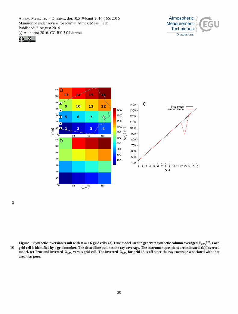
The LSQR algorithm was tested using a synthetic realistic scenario. Synthetic data 𝑋𝐶𝑂2

𝑐𝑜𝑙 were generated from a

true model comprising of known 𝑋𝐶𝑂2 at each grid point using the real geometry matrix 𝐿 , which contained the actual

instrument positions and measured ranges. 𝑋𝐶𝑂2 of the true model were starting at 380 ppm at grid 1 and increasing by 60 ppm

per increase in grid number (Fig. 5a). By running the inversion with varying number of grid cells the viable number of grid

cells was found to be between 𝑛 = 4 up to 36 without considerable loss of capability to recover the true 𝑋𝐶𝑂2 (Fig. 5b). 5

For 𝑛 > 36 the inverted 𝑋𝐶𝑂2 oscillated, that is, they were over and under shooting the true 𝑋𝐶𝑂2

.

For the real data, however, already for 𝑛 > 16 the inversion yielded unreasonable high 𝑋𝐶𝑂2, indicating an

oscillation. The inverse problem is over determined since 𝑚 ≫ 𝑛, i.e. the number of beam paths traversing most of the grid

cells is much higher than any practical number of grid cells usable for the inversion. Increasing the number of grid cells would

reduce the number of rays traversing a given grid cell, but the problem would become highly non-linear. Generally, a viable 10

strategy to tackle non-linearity in situations like that is a gradual introduction of non-linearity, such as by splitting up the

inversion into sub-steps, using a starting model close enough to the true solution at each step (Queißer et al., 2012). With each

increase in sub-step, the starting model contains more small-scale information. This approach was tested in the real data

inversion. Starting with 𝑛 = 4 grid cells, the inversion result was interpolated, smoothed and used as the starting model for the

inversion with (𝑛𝑥 + 1)2 grid cells. At 𝑛 = 25 the location of the peak 𝑋𝐶𝑂2were in strong disagreement with the LICOR data, 15

indicating that the inversion was trapped in a local minimum. A similar outcome was obtained by reducing the number of rays

used for the inversion (using every 2nd up to every 10th ray).

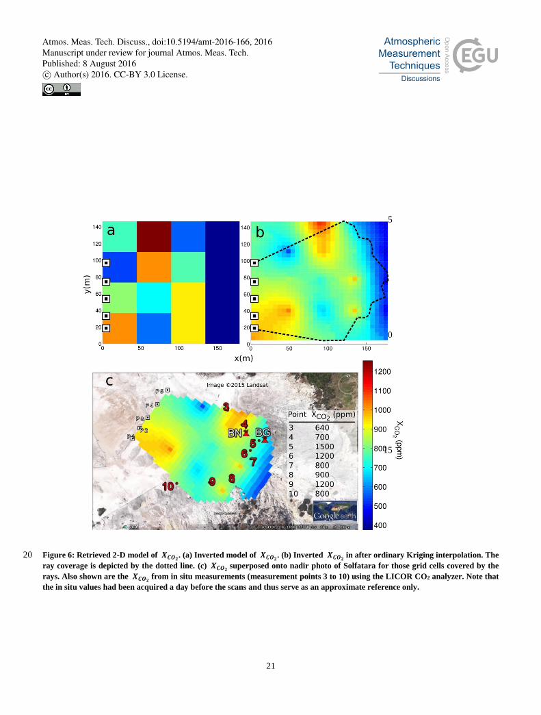
That left 𝑛 = 16 the maximum feasible number of grid cells for a robust inversion. The resulting grid length was

∆𝑥 = 38 m and ∆𝑦 = 33 m. As for the synthetic tests, a constant 𝑋𝐶𝑂2, the mean of the raw data (Fig. 4), was used as a starting

model. The inversion result is shown in Fig. 6a. To increase spatial resolution the inverted model was interpolated onto a grid 20

with grid spacing ∆𝑥/8 and ∆𝑦/8 using ordinary Kriging interpolation (Oliver, 1996). The result is shown in Fig. 6b.

Overlaying the 2-D map of CO2 mixing ratios with the map of Solfatara reveals a zone of increased anomalous CO2 degassing

activity along the southeastern edge of Solfatara, which is in reasonable agreement with in situ data from the LICOR CO2

analyzer (Fig. 6c).

The resulting 2-D map of CO2 mixing ratios was used to compute the CO2 flux. Since zones with poor ray coverage 25

were prone to inversion artifacts (see Fig. 4c) zones without ray coverage were excluded from integration. The plume transport

speed was estimated to be 1.1 ± 0.2 m s-1. The plume speed uncertainty was retrieved from the standard deviation of various

plume speeds retrieved from different tracks carried out across the plume. To estimate the flux uncertainty (Eq. 10), a constant

∆𝑋𝐶𝑂2,𝑝𝑙 = max (∆𝑋𝐶𝑂2,𝑎𝑣) was considered (maximum error of all five scans). Using Eq. (8) the resulting CO2 flux was

computed as 12.8 ± 3.3 kg s-1 (± 1 SD) or 1106 ± 288 tons day-1.

30


8

4 Discussion

The retrieved 2-D map (Fig. 6c) indicates an elongated zone of intense anomalous degassing along the eastern edge of the

Solfatara crater. Encouragingly, this is a persistent feature in different inversions performed with different number of grid cells

and beam paths (and thus degree of non-linearity) and underpins that it is real. Previous measurements sampling the Solfatara

area with accumulation chambers yielded an increased anomalous CO2 degassing activity in the corresponding area too 5

(Granieri et al., 2010; Tassi et al., 2013; Bagnato et al., 2014). The retrieved elongated zone of anomalous CO2 degassing

likely encompasses at least two major vents (Fig. 6c). The locations of the peaks in CO2 mixing ratio in Fig. 6c fairly agree

with the 1-D input data. For instance, the peak near the center of the crater corresponds to the peak near 26° in the first scan in

Fig. 3a. The second scan (Fig. 3b) indicates a rather abrupt decrease in 𝑋𝐶𝑂2,𝑎𝑣 at 28°, in line with the edge of the zone of

elevated CO2 concentrations at the crater center (Fig. 6c). This central degassing feature is coherent with results of recent 10

campaigns (Granieri et al., 2010; Tassi et al., 2013; Bagnato et al., 2014). The symmetric increase in 𝑋𝐶𝑂2,𝑎𝑣 near 9° in Fig.

3d corresponds to the position of the local peak in 𝑋𝐶𝑂2between in situ points 7 and 8 in Fig. 6c. Provided sufficient ray

coverage and angle diversity, which is the case for the zones away from the edges of the 2-D map, disagreement between the

peaks in the 1-D data (Fig. 3) and those in the 2-D map (Fig. 6) are likely due to physical fluctuations in CO2 concentration.

The plume was assumed to be “frozen”, but the measurement duration of 142 min was certainly larger than the time scale of 15

alterations in the dispersion pattern of the plume. During acquisition one could visually identify at least 5 small vents emitting

water vapor and therefore most likely also CO2. Though not recovered due to the limited spatial resolution of the inversion

this advocates that there are in fact separate vents south of the main vents, near the edge of the Solfatara crater.

Retrieved 𝑋𝐶𝑂2 peak near 1300 ppm (2 m above ground), in line with the in situ LICOR data, although not spatially

matching them in places. Again, this can be explained by the fact that the in situ values were acquired the day before so that 20

local wind and thus dispersion patterns were different. Nevertheless, both the LICOR in situ data and the inversion result

indicate high 𝑋𝐶𝑂2 near the main vents and along the crater edge. Near the main vents highest CO2 mixing ratios in the 2-D

map are located ca. 20 m west of BN. In fact, the whole zone of high 𝑋𝐶𝑂2 is shifted 20 m northwest from where one would

expect it. Since the predominant wind direction at the time of acquisition was around 300°, to first order one would expect the

CO2 to disperse rather towards southeast, along the crater edge. The main vent area was at the edge of the scanned area. Note 25

that the relative inversion residual ‖𝑎 − 𝐿𝑐‖/‖𝑎‖ was 0.18, which means on average 18% of 𝑋𝐶𝑂2

𝑐𝑜𝑙 are unexplained by the

model in Fig. 6a. This mismatch is therefore likely due to poor ray coverage and angle diversity for the zone containing the

main vents, since the acquisition focused on the zone south of the main vents. Possibly, but less likely, CO2 was advected

slightly towards west due to dispersive mechanism related to local wind eddies decoupled from the main wind direction. These

dispersive mechanisms take place in any case and make a distinction between CO2 from the main vents and the surrounding 30

diffuse degassing challenging. For that reason, in future acquisitions at that site the region of interest shall be scanned from

instrument positions aligned along a half circle around the zone rather than using a “flat” scan geometry as chosen here.


9

For a comparison, CO2 fluxes were computed directly from the 1-D profiles, that is, similar to Eq. (8) but using path

amounts, ignoring any heterogeneity in the CO2 distribution. The average flux of all five scans (1055 ± 389 tons/day) is in

good agreement with the result obtained from the 2-D map (1106 ± 288 tons/day).. Note that disagreement with the flux result

from the 2-D map may partly be due to the frozen plume assumption, since this assumption is better fulfilled for the acquisition

of a single 1-D profile, which takes much less time. Future scans shall thus be acquired with higher scan velocity or from 5

further away.

Yet, both the CO2 flux from the 2-D map and from the 1-D profiles are higher than fluxes previously estimated. To

our knowledge, all former studies except one (Pedone et al., 2014) inferred 𝑋𝐶𝑂2 and hence CO2 fluxes from a grid of point

measurements, which may have missed degassing activity in between the measurement points and so tended to yield lower

flux values. Spatially comprehensive sounding by Pedone et al. (2014) resulted in a CO2 flux of only ~300 tons/day in early 10

2013, however, it focused on the area around the Solfatara main vents, that is, 8000 m2. In this study the area considered for

flux computation was over 21000 m2. The average degassing rate at Solfatara has been increasing by ~9% each year over the

past 10 years or so (Chiodini et al., 2010; d’Auria, 2015). Extrapolating the 300 tons/day would yield a flux of 390 tons/day

in early 2016. Integrating CO2 mixing ratios of the area around the main vents only (bounded to the south by in situ point 6,

Fig. 6c) yields a flux of 399 ± 104 tons/day of CO2, in excellent agreement with the extrapolated flux. However, as mentioned 15

before, CO2 from the main vents mixes with surrounding volcanic CO2 and furthermore the scans focused on the area south of

the main vents (poor ray coverage at BN and BG). So this value should be interpreted with care. It deems to be reasonable to

exclude the zone of high anomalous degassing in the north of the 2-D map, which leads to a flux of 675 ± 175 tons/day,

representing any degassing activity (vented and diffuse) within the investigated area, excluding the main vent area (BN and

BG). This magnitude equals roughly 45% of the total CO2 flux of the DDS (diffuse degassing structure) reported by Granieri 20

et al. (2003), 13 years prior to this study.

All five scans were performed one-sided, i.e. from a single half space, as often the case in geophysical tomography

problems (e.g. Hobro et al., 2003). This is not ideal for any inversion technique as it makes the inverse problem highly non-

linear with a non-unique solution, meaning that many models may explain the observed data equally well. However, for

Solfatara there is an abundance of hard data available, which extremely facilitated the rejection of unlikely models. This case 25

therefore enabled to demonstrate that one may obtain useful tomographic results from one-sided scanning of a degassing

feature. The inverted model is missing small-scale features, since to linearize the inversion the grid spacing had to be rather

coarse. Yet, given the fair agreement with the hard data, the inverted 2-D model (Fig. 6c) is quantitatively sound and outlines

the geometry of the diffuse degassing probed at Solfatara. Future measurements of this type at Solfatara are envisaged,

including a more systematic study, using a wider variety of viewing angles, which will allow a more quantitative picture as to 30

which extent this method is useful for one-sided tomography of highly non-isotropic volcanic CO2 plumes. In particular, we

expect an enlarged angle diversity to increase the maximum number of grids usable for stable inversion, boosting 2-D

resolution. The outcome indicates this method to be particularly useful for future measurement campaigns using hard target

DIAL to scan volcanic plumes from an aircraft or similar acquisition geometries sensing other types of gas emission.


10

5 Conclusions

As magmatic CO2 degassing rates are tracers for the dynamics and chemistry of the magma plumbing system beneath Campi

Flegrei and at volcanic areas in general, a comprehensive quantification of magmatic CO2 degassing strength is of interest for

volcanology and of vital importance for civil protection. 5

Scanning hard target DIAL measurements have been performed at Solfatara crater (Campi Flegrei, Italy), which

allowed an inclusive measurement of CO2 amounts in the form of 1-D profiles of CO2 path amounts. From the 1-D profiles a

2-D map of CO2 mixing ratios has been reconstructed outlining the main CO2 distribution. Such a map is useful to

geometrically correct the CO2 flux obtained from 1-D concentration profiles for heterogeneous CO2 distribution. Since it was

in line with in situ hard data, the 2-D map was directly used to retrieve the CO2 flux, which is compatible with previous results. 10

The 1-D profiles have been acquired from a single half space, which indicates this tomography method to be beneficial for

scanning strongly non-isotropic CO2 distributions, such as diffuse emissions, that can be viewed from limited angles only. To

fully assess the potential of this method, future acquisitions should involve different scanning geometries, potentially allowing

for an enhanced resolution of the 2-D map and thus more accurate gas flux estimation.

15

Acknowledgments

The research leading to these results has received funding from the European Research Council under the European Union’s

Seventh Framework Programme (FP/2007-2013)/ERC Grant Agreement n. 279802. Our gratitude goes to Rosario Avino and

Antonio Carandente (INGV Osservatorio Vesuviano), who sampled the in situ CO2 mixing ratios. We thank Grant Allen

(NASA Goddard) and Luca Fiorani (ENEA) for sharing extremely valuable experiences in LIDAR development with us. 20

References

Aiuppa, A., Burton, M., Allard, P., Caltabiano, T., Giudice, G., Gurrieri, S., Liuzzo, M., Salerno, G.: First observational

evidence for the CO2-driven origin of Stromboli’s major explosions, Solid Earth, 2, 135-142, 2011. 25


11

Aiuppa, A., Tamburello, G., Di Napoli, R., Cardellini, C., Chiodini, G., Giudice, G., Grassa, F., and Pedone, M.: First

observations of the fumarolic gas output from a restless caldera: Implications for the current period of unrest (2005–2013) at

Campi Flegrei, Geochem. Geophys. Geosyst., 14, 4153-4169, 2013.

Aiuppa, A., Fiorani, L., Santoro, S., Parracino, S., Nuvoli, M., Chiodini, G., Minopoli, C., and Tamburello, G.: New ground-5

based lidar enables volcanic CO2 flux measurements, Sci. Rep., 5, 13614; doi: 10.1038/srep13614, 2015.

Amediek, A., Fix, A., Wirth, M., and Ehret, G.: Development of an OPO system at 1.57 µm for integrated path DIAL

measurement of atmospheric carbon dioxide, Appl. Phys. B, 92, 295-302, 2008.

10

d’Auria, L.: Update sullo stato dei Campi Flegrei, INGV, Sezione di Napoli, Report, available at

ftp://ftp.ingv.it/pro/web_ingv/Convegno_Struttura%20_Vulcani/presentazioni/15_D'auria_CampiFlegrei/dauria_cf.pdf,

accessed in May 2016, 2015.

Bagnato, E., Barra, M., Cardellini, C., Chiodini, G., Parello, F., and Sprovieri, M.: First combined flux chamber survey of 15

mercury and CO2 emissions from soil diffuse degassing at Solfatara of Pozzuoli crater, Campi Flegrei (Italy): Mapping and

quantification of gas release, J. Volcanol. Geotherm. Res., 289, 26-40 2014.

Baubron, J. C., Allard, P., Sabroux, J. C., Tedesco, D., Toutain, J.P.: Soil gas emanations as precursory indicators of

volcanic eruptions, J. Geol. Soc. London 148, 571-576, 1991. 20

Burton, M. R., Sawyer, G. M., and Granieri, D.: Deep carbon emissions from Volcanoes, Rev. Mineral. Geochem., 75, 323-

354, 2013.

Carapezza, M. L., Inguaggiato, S., Brusca, L., and Longo, M.: Geochemical precursors of the activity of an open-conduit 25

volcano: The Stromboli 2002-2003 eruptive events, Geophys. Res. Lett., 31, L07620, 2004.

Chiodini, G., Baldini, A., Barberi, F., Carapezza, M. L., Cardellini, C., Frondini, F., Granieri, D., and Ranaldi, M.: Carbon

dioxide degassing at Latera caldera (Italy): Evidence of geothermal reservoir and evaluation of its potential energy, J. Geophys.

Res., 112, B12204, 2007. 30

Chiodini, G., Caliro, S., Cardellini, C., Granieri, D., Avino, R., Baldini, A., Donnini, M., and C. Minopoli.: Long-term

variations of the Campi Flegrei, Italy, volcanic system as revealed by the monitoring of hydrothermal activity, J. Geophys.

Res., 115, B03205, doi:10.1029/2008JB006258, 2010.


12

Chiodini, G., Pappalardo, L., Aiuppa, A., and Caliro, S.: The geological CO2 degassing history of a long-lived caldera,

Geology, 43, 767-770, 2015.

Diaz, J. A., Pieri, D., Arkin, C. R., Gore, E., Griffin, T. P., Fladeland, M., Bland, G., Soto, C., Madrigal, Y., Castillo, D., Rojas, 5

E., and Achi, S.: Utilization of in situ airborne MS-based instrumentation for the study of gaseous emissions at active

volcanoes, Int. J. Mass Spectrom., 295, 105-112, 2010.

Dobler, J. T., Harrison, F. W., Browell, E. V., Lin, B., McGregor, D., Kooi, S., Choi, Y., and Ismail, S.: Atmospheric CO2

column measurements with an airborne intensity-modulated continuous-wave 1.57-micron fiber laser lidar, Appl. Optics, 52, 10

2874-2894, 2013.

Frezzotti, M.-L. and Touret, J. L. R.: CO2, carbonate-rich melts, and brines in the mantle, Geosci. Front., 5, 697-710, 2014.

Galle, B., Johansson, M., Rivera, C., Zhang, Y., Kihlman, M., Kern, C., Lehmann. T., Platt, U., Arellano, and S., Hidalgo, S.: 15

Network for Observation of Volcanic and Atmospheric Change (NOVAC)-A global network for volcanic gas monitoring:

Network layout and instrument description, J. Geophys. Res., 115, D05304, doi:10.1029/2009JD011823, 2010.

Gerlach, T. M., Delgado, H., McGee, K. A., Doukas, M. P., Venegas, J. J., Cárdenas, L.: Application of the LI-COR CO2

analyzer to volcanic plumes: A case study, volcán Popocatépetl, Mexico, June 7 and 10, 1995, J. Geophys. Res., 102, 8005-20

8019, 1997.

Granieri, D., Chiodini, G., Marzocchi, W., and Avino, R.: Continuous monitoring of CO2 soil diffuse degassing at Phlegraean

Fields (Italy): influence of environmental and volcanic parameters, Earth Planet. Sci. Lett., 212, 167-179, 2003.

25

Granieri, D., Avino, R., Chiodini, G.: Carbon dioxide diffuse emission from the soil: ten years of observations at Vesuvio

and Campi Flegrei (Pozzuoli), and linkages with volcanic activity, Bull. Volcanol., 72, 103–118, doi:10.1007/s00445-009-

0304-8, 2010.

Granieri, D., Carapezza, M. L., Barberi, F., Ranaldi, M., Ricci, T., and L. Tarchini.: Atmospheric dispersion of natural carbon 30

dioxide emissions on Vulcano Island, Italy, J. Geophys. Res. Solid Earth, 119, doi:10.1002/2013JB010688, 2014.

Hards, V. L.: Volcanic contributions to the global carbon cycle, British Geological Survey Occasional Report No. 10, 26pp.,

2005.


13

Hobro, J. W. D., Singh, S. C., and Minshull, T. A.: Three-dimensional tomographic inversion of combined reflection and

refraction seismic traveltime data, Geophys. J. Int., 152, 79-93, 2003.

Johansson, M., Galle, B., Rivera, B., and Zhang, Y.: Tomographic reconstruction of gas plumes using scanning DOAS, Bull. 5

Volcanol., 71, 1169-1178, 2009.

Kameyama, S., Imaki, M., Hirano, Y., Ueno, S., Kawakami, S., Sakaizawa, D., and Nakajima, M.: Development of 1.6 μm

continuous-wave modulation hard-target differential absorption lidar system for CO2 sensing, Opt. Lett., 34, 1513-1515, 2009.

10

Kazahaya, R., Mori, T., Kazahaya, K., and Hirabayashi, J.: Computed tomography reconstruction of SO2concentration

distribution in the volcanic plume of Miyakejima, Japan, by airborne traverse technique using three UV spectrometers,

Geophys. Res. Lett., 35, L13816, 2008.

Koch, G. J, Barnes, B. W., Petros, M., Beyon, J. Y., Amzajerdian, F., Yu, J., Davis, R. E, Ismail, S., Vay, S., Kavaya, M. J, 15

and Singh, U. N.: Coherent differential absorption lidar measurements of CO2, Appl. Optics, 43, 5092-5099, 2004.

La Spina, G., Burton, M., and de Vitturi, M.: Temperature evolution during magma ascent in basaltic effusive eruptions: A

numerical application to Stromboli volcano, Earth Planet. Sci. Lett., 426, 89-100, 2015.

20

Lee, H, Muirhead, J. D, Fischer, T. P, Ebinger, C. J, Kattenhorn, S. A, Sharp, Z. D., and Kianji, G.: Massive and prolonged

deep carbon emissions associated with continental rifting, Nature Geosci., 9, 145-149, 2016.

Lewicki, J. L., Bergfeld, D., Cardellini, C., Chiodini, G., Granieri, D., Varley, N., Werner, C.: Comparative soil CO2 flux

measurements and geostatistical estimation methods on Masaya volcano, Nicaragua, Bull. Volcanol., 68, 76-90, 2005. 25

McGee, K. A., Doukas, M. P., McGimsey, R. G., Neal, C. A., and Wessels, R. L.: Atmospheric contribution of gas emissions

from Augustine volcano, Alaska during the 2006 eruption, Geophys. Res. Lett., 35, L03306, doi:10.1029/2007GL032301,

2008.

30

MacKerrow, E. P, Schmitt, M. J., and Thompson, D. C.: Effect of speckle on lidar pulse-pair ratio statistics, Appl. Optics, 36,

8650-8669, 1997.


14

Menzies, R. T. and Chahine, M. T.: Remote Atmospheric Sensing with an Airborne Laser Absorption Spectrometer, Appl.

Opt., 13, 2840-2849, 1974.

Oliver, M. A.: Kriging: a method of estimation for environmental and rare disease data, Geo. Soc., London, Special

Publications, 113, 245-254, doi: 10.1144/GSL.SP.1996.113.01.21, 1996. 5

Pedone, M., Aiuppa, A., Giudice, G., Grassa, F., Cardellini, C., Chiodini, G., and Valenza, M.: Volcanic CO2 flux measurement

at Campi Flegrei by Tunable Diode Laser absorption Spectroscopy, Bull. Volc., 76, doi: 10.1007/s00445-014-0812-z, 2014.

Platt, U., Lübke, P., Kuhn, J., Bobrowski, N., Prata, F., Burton, M., Kern, C.: Quantitative imaging of volcanic plumes -Results, 10

needs, and future trends, J. Volcanol. Geotherm. Res., 300, 7-21, 2015.

Petrazzuoli, S. M., Troise, C., Pingue, F., and DeNatale, G.: The mechanisms of Campi Flegrei unrests as related to plastic

behaviour of the caldera borders, Ann. Geofis., 42, 529-544, 1999.

15

Queißer, M. and Singh, S. C.: Full Waveform Inversion for time lapse quantitative monitoring of CO2 storage, Geophys.

Prosp., 61, 537-555, 2012.

Queißer, M., Burton, M., and Fiorani, L.: Differential absorption lidar for volcanic CO2 sensing tested in an unstable

atmosphere, Opt. Express, 23, 6634-6644, 2015a. 20

Queißer, M , Granieri, D., Burton, M., La Spina, A., Salerno, G., Avino, R., and Fiorani, L.: Intercomparing CO2 amounts

from dispersion modeling, 1.6 µm differential absorption lidar and open path FTIR at a natural CO2 release at Caldara di

Manziana, Italy, Atmos. Meas. Tech. Discuss., 8, 4325-4345, 2015b.

25

Rothman, L. S., Gordon, I. E., Babikov, Y., Barbe, A., Benner, D. C., Bernath, P. F., Birk, M, Bizzocchi, L., Boudon, V.,

Brown, L. R., Campargue, A., Chanc, K., Coudert, L., Devi, V. M., Drouin, B. J., Fayt, A., Flaud, J.-M., Gamache, R. R.,

Harrison, J., Hartmann, J.-M., Hill, C., Hodges, J. T., Jacquemart, D., Jolly, A., Lamouroux, J., LeRoy, R. J., Li, G., Long, D.,

Mackie, C. J., Massie, S. T., Mikhailenko, S., Müller, H. S. P., Naumenko, O. V., Nikitin, A. V., Orphal, J., Perevalov, V.,

Perrin, A., Polovtseva, E. R., Richard, C., Smith, M. A. H., Starikova, E., Sung, K., Tashkun, S., Tennyson, J., Toon, G. C., 30

Tyuterev, V. G., Auwera, J. V., and Wagner, G.: The HITRAN 2012 Molecular Spectroscopic Database, J. Quant. Spectrosc.

Ra., 130, 4-50, 2013.


15

Sakaizawa, D., Nagasawa, C., Nagai, T., Abo, M., Shibata, Y., Nakazato, M.,and Sakai, T.: Development of a 1.6 μm

differential absorption lidar with a quasi-phase-matching optical parametric oscillator and photon-counting detector for the

vertical CO2 profile, Appl. Optics, 48, 748-757, 2009.

Sakaizawa, D., Kawakami, S., Nakajiama, M., Tanaka, T., Morino, I., and Uchino, O.: An airborne amplitude modulated 1.57 5

µm differential laser absorption spectrometer: simultaneous measurement of partial column-averaged dry air mixing ratio of

CO2 and target range, Atmos. Meas. Tech., 6, 387-396, 2013.

Scarpati, C., Cole, P., and Perrotta, A.: The Neapolitan Yellow Tuff- A large volume multiphase eruption from Campi Flegrei,

Southern Italy, Bull. Volcanol., 55, 343-356, 1993. 10

Tassi, F, Nisi, B., Cardellini, C., Capecchiacci, F., Donnini, M., Vaselli, O., Avino, R., and Chiodini, G.: Diffuse soil

emission of hydrothermal gases (CO2, CH4 and C6H6) at the Solfatara crater (Phlegraean Fields, southern Italy), Appl.

Geochem., 35, 142-153, 2013.

15

Weibring, P., Edner, H., Svanberg, S., Cecchi, G., Pantani, L., Ferrara, R., Caltabiano, T.: Monitoring of volcanic sulphur

dioxide emissions using differential absorption lidar (DIAL), differential optical absorption spectroscopy (DOAS), and

correlation spectroscopy (COSPEC), Appl. Phys. B, 67, 419-426, 1998.

Wright, T. E., Burton, M. R., Pyle, D. M, and Caltabiano, T.: Scanning tomography of SO2 distribution in a volcanic gas plume, 20

Geophys. Res. Lett., 35, L17811, doi: 10.1029/2008GL034640, 2008.

25

30


16

Figures

5

10

15

Figure 1: Geography and measurement geometry. (a) Location of the Solfatara crater as part of the volcanic area of Campi Flegrei,

near Naples (Italy). (b) Nadir photo of Solfatara crater. The rectangle contains the region of interest. (c) Zoom of area outlined by

the rectangle depicting the five instrument positions P1 to P5 with the following UTM-coordinates: P1: (427476, 4519921), P2:

(427485, 4519935), P3: (427495, 4519949), P4: (427507, 4519967), P5: (427520, 4519986). Also shown are the respective range vectors 20 (rays) for all five scans and the numbered locations of the LICOR measurements. (d) Photo taken during the scan at P5 looking

towards east. The largest clouds of condensed water aerosol appeared near the main vents (Bocca Nuova, BN and Bocca Grande,

BG) on the left. The CO2DIAL, visible in the lower right corner, comprised of the tripod carrying the telescope (with transmitter

unit) and the main unit (red box).

25


17

Figure 2: Scheme of the CO2 DIAL as used for this experiment. EOM: Electro-optical modulator, DLEM: range finder module,

EDFA: Erbium doped fiber amplifier. ADC: analog-to-digital converter, DAC: digital-to-analog converter. The CO2 cell is used to

calibrate the seed laser wavelengths. To minimize hard target and turbulence related speckle noise the collimator used had a 5 relatively high divergence of 1.7 mrad while the telescope field of view was 1.5 mrad. For mechanical reasons the optical band pass

filter was mounted before the collimating lens. The change in transmission spectrum can be neglected.


18

Figure 3: 1-D profiles of 𝑿𝑪𝑶𝟐,𝒂𝒗, the total (not background corrected) CO2 mixing ratios, derived by dividing the path amounts

𝑿𝑪𝑶𝟐

𝒄𝒐𝒍 (ppm.m) per angle by the associated range. Each value therefore represents a column-averaged concentration. Each point

corresponds to 784 ms integration time. For each profile and heading ranges are indicated by the red dashed line. (a) Profile acquired

between 9:35:36 and 9:41:54. (b) Profile acquired between 10:04:08 and 10:10:54. (c) Profile acquired between 10:31:24 and 5 10:37:28. (d) Profile acquired between 11:01:46 and 11:07:46. (e) Profile acquired between 11:50:39 and 11:57:15. The grey envelope

depicts precision (1 SD, Eq. 3).


19

5

10

15

Figure 4: Contour plot of 𝑿𝑪𝑶𝟐,𝒂𝒗 (𝑿𝑪𝑶𝟐

𝒄𝒐𝒍 divided by the range) for all 627 beam paths. Also shown are the instrument positions

(squares on y-axis) starting with P1 at 𝒚 =20 m. The data has been regridded on a regular grid of 90×90 points using natural

interpolation. One would expect high anomalous CO2 mixing ratios near the main vents (BN, BG near 𝒙 =120 m, 𝒚 =140 m) and 20 the southern part of the area. Low anomalous CO2 mixing ratios are to be expected in the northwestern part. Note that due to the

abundance of data some data points were masking each other. They were thus averaged, leading to a maximum mixing ratio lower

than actually observed (e.g. in Fig. 3b).

25


20

5

Figure 5: Synthetic inversion result with 𝒏 = 𝟏𝟔 grid cells. (a) True model used to generate synthetic column averaged 𝑿𝑪𝑶𝟐

𝒄𝒐𝒍. Each

grid cell is identified by a grid number. The dotted line outlines the ray coverage. The instrument positions are indicated. (b) Inverted 10 model. (c) True and inverted 𝑿𝑪𝑶𝟐

versus grid cell. The inverted 𝑿𝑪𝑶𝟐 for grid 13 is off since the ray coverage associated with that

area was poor.


21

5

10

15

Figure 6: Retrieved 2-D model of 𝑿𝑪𝑶𝟐. (a) Inverted model of 𝑿𝑪𝑶𝟐

. (b) Inverted 𝑿𝑪𝑶𝟐 in after ordinary Kriging interpolation. The 20

ray coverage is depicted by the dotted line. (c) 𝑿𝑪𝑶𝟐 superposed onto nadir photo of Solfatara for those grid cells covered by the

rays. Also shown are the 𝑿𝑪𝑶𝟐 from in situ measurements (measurement points 3 to 10) using the LICOR CO2 analyzer. Note that

the in situ values had been acquired a day before the scans and thus serve as an approximate reference only.


Documents

2-D tomography of volcanic CO from scanning hard target ...€¦ · 2-D tomography of volcanic CO 2 from scanning hard target differential absorption LIDAR: The case of Solfatara,