Transp Porous MedDOI 10.1007/s11242-010-9582-z

Effects of CO2 Compressibility on CO2 Storagein Deep Saline Aquifers

Victor Vilarrasa · Diogo Bolster · Marco Dentz ·Sebastia Olivella · Jesus Carrera

Received: 3 August 2009 / Accepted: 5 April 2010© Springer Science+Business Media B.V. 2010

Abstract The injection of supercritical CO2 in deep saline aquifers leads to the formationof a CO2 plume that tends to float above the formation brine. As pressure builds up, CO2

properties, i.e. density and viscosity, can vary significantly. Current analytical solutions donot account for CO2 compressibility. In this article, we investigate numerically and analyti-cally the effect of this variability on the position of the interface between the CO2-rich phaseand the formation brine. We introduce a correction to account for CO2 compressibility (den-sity variations) and viscosity variations in current analytical solutions. We find that the errorin the interface position caused by neglecting CO2 compressibility is relatively small whenviscous forces dominate. However, it can become significant when gravity forces dominate,which is likely to occur at late times of injection.

Keywords Two phase flow · CO2 density · Analytical solution · Interface · Gravity forces

Nomenclaturecr Rock compressibilitycα Compressibility of fluid α (α = c, w)d Aquifer thicknessErel Relative error of the interface positiong Gravityhw Hydraulic head of waterk Intrinsic permeabilitykrα α-Phase relative permeability (α = c, w)N Gravity number

V. Vilarrasa · M. Dentz · J. CarreraInstitute of Environmental Assessment and Water Research, GHS, IDAEA, CSIC, Barcelona, Spain

V. Vilarrasa (B) · D. Bolster · S. OlivellaDepartment of Geotechnical Engineering and Geosciences, Technical University of Catalonia (UPC),Barcelona, Spaine-mail: victor.vilarrasa@upc.edu

123

V. Vilarrasa et al.

Pt0 Fluid pressure at the top of the aquifer prior to injectionPDT Fluid pressure for Dentz and Tartakovsky (2009a) approachPDT Vertically averaged fluid pressure for Dentz and Tartakovsky (2009a) approachPN Vertically averaged fluid pressure for Nordbotten et al. (2005) approachP0 Vertically averaged fluid pressure prior to injectionPα Fluid pressure of α-phase (α = c, w)Qm CO2 mass flow rateQ0 CO2 volumetric flow rateqα Volumetric flux of α-phase (α = c, w)R Radius of influenceRc CO2 plume radius at the top of the aquifer for compressible CO2

Ri CO2 plume radius at the top of the aquifer for incompressible CO2

r Radial distancer0 CO2 plume radius at the top of the aquiferrb CO2 plume radius at the base of the aquiferrc Characteristic lengthrw Injection well radiusSs Specific storage coefficientSrw Residual saturation of the formation brineSα Saturation of α-phase (α = c, w)t Timez Vertical coordinatez0 Depth of the top of the aquiferzb Depth of the base of the aquiferV CO2 plume volumeα Phase index, c CO2 and w brineβ CO2 compressibilityεv Volumetric strainγcw A dimensionless parameter that measures the relative importance of viscous

and gravity forcesλα Mobility of α-phase (α = c, w)μα Viscosity of α-phase (α = c, w)ρ0 CO2 density at the reference pressure Pt0ρ1 Constant for the CO2 densityρc Mean CO2 densityρcDT

Mean CO2 density for Dentz and Tartakovsky (2009a) approachρcN

Mean CO2 density for Nordbotten et al. (2005) approachρα Density of α-phase (α = c, w)σ ′ Effective stressφ Porosityζ Interface position from the bottom of the aquifer

1 Introduction

Carbon dioxide (CO2) sequestration in deep geological formations is considered a prom-ising mitigation solution for reducing greenhouse gas emissions to the atmosphere.Although this technology is relatively new, wide experience is available in the field ofmultiphase fluid injection [e.g. the injection of CO2 for enhanced oil recovery (Lake 1989;

123

CO2 Compressibility Effects

Cantucci et al. 2009), production and storage of natural gas in aquifers (Dake 1978; Katz andLee 1990), gravity currents (Huppert and Woods 1995; Lyle et al. 2005) and disposal of liquidwaste (Tsang et al. 2008)]. Various types of geological formations can be considered for CO2

sequestration. These include unminable coal seams, depleted oil and gas reservoirs and deepsaline aquifers. The latter have received particular attention due to their high CO2 storagecapacity (Bachu and Adams 2003). Viable saline aquifers are typically at depths greater than800 m. Pressure and temperature conditions in such aquifers ensure that the density of CO2

is relatively high (Hitchon et al. 1999).Several sources of uncertainty associated with multiphase flows exist at these depths.

These include those often encountered in other subsurface flows such as the impact of heter-ogeneity of geological media, e.g. (Neuweiller et al. 2003; Bolster et al. 2009b), variabilityand lack of knowledge of multiphase flow parameters (e.g. van Genuchten and Brooks–Coreymodels). Beyond these difficulties, the properties of supercritical CO2, such as density andviscosity, can vary substantially (Garcia 2003; Garcia and Pruess 2003; Bachu 2003) makingthe assumption of incompressibility questionable.

Two analytical solutions have been proposed for the position of the interface between theCO2-rich phase and the formation brine: the Nordbotten et al. (2005) solution and the Dentzand Tartakovsky (2009a) solution. Both assume an abrupt interface between phases. Bothsolutions neglect CO2 dissolution into the brine, so the effect of convective cells (Ennis-Kingand Paterson 2005; Hidalgo and Carrera 2009; Riaz et al. 2006) on the front propagation is nottaken into account. Each phase has constant density and viscosity. The shape of the solutionby Nordbotten et al. (2005) depends on the viscosity of both CO2 and brine, while the onederived by Dentz and Tartakovsky (2009a) depends on both the density and viscosity dif-ferences between the two phases. The validity of these sharp interface solutions has beendiscussed in, e.g., Dentz and Tartakovsky (2009a); Lu et al. (2009); Dentz and Tartakovsky(2009b).

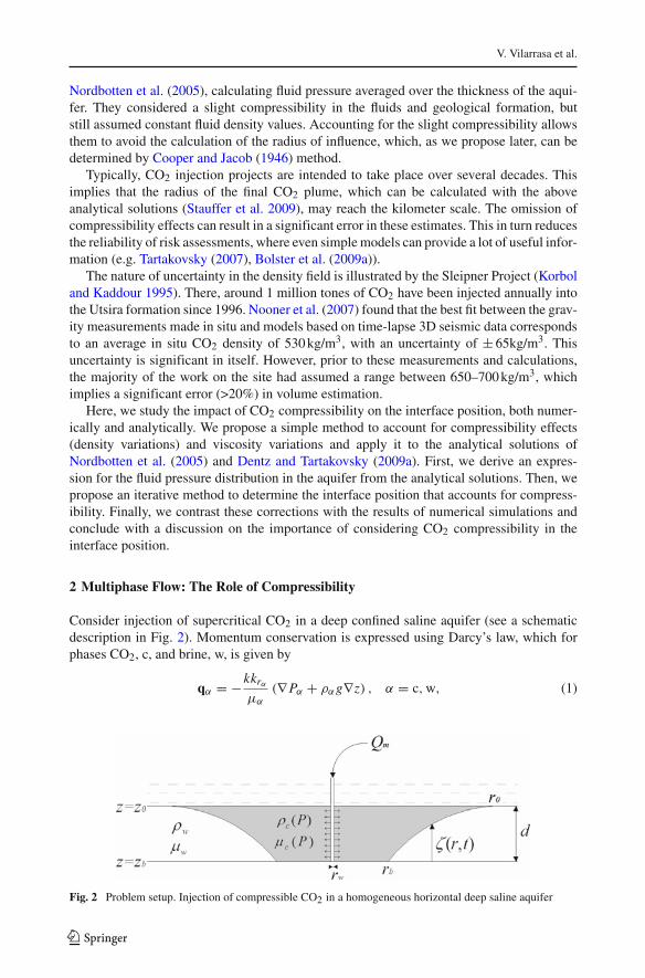
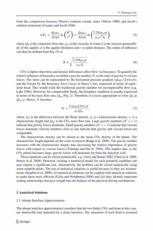
The injection of CO2 causes an increase in fluid pressure, and displaces the formationbrine laterally. This brine can migrate out of the aquifer if the aquifer is open, causing sali-nization of other formations such as fresh water aquifers. In contrast, if the aquifer has verylow-permeability boundaries, the storage capacity will be related exclusively to rock andfluid compressibility (Zhou et al. 2008). In the latter case, fluid pressure will increase dra-matically and this can lead to geomechanical damage of the caprock (Rutqvist et al. 2007).Additionally, this pressure buildup during injection gives rise to a wide range of CO2 densityvalues within the CO2 plume (Fig. 1). As density changes are directly related to changes involume, the interface position will be affected by compressibility. However, neither of thecurrent analytical solutions for the interface location acknowledge changes in CO2 density.

The evolution of fluid pressure during CO2 injection has been studied by several authors,e.g. (Saripalli and McGrail 2002; Mathias et al. 2008). Mathias et al. (2008) followed

715

700

685670 655 640

Fig. 1 CO2 density (kg/m3) within the CO2 plume resulting from a numerical simulation that acknowledgesCO2 compressibility

123

V. Vilarrasa et al.

Nordbotten et al. (2005), calculating fluid pressure averaged over the thickness of the aqui-fer. They considered a slight compressibility in the fluids and geological formation, butstill assumed constant fluid density values. Accounting for the slight compressibility allowsthem to avoid the calculation of the radius of influence, which, as we propose later, can bedetermined by Cooper and Jacob (1946) method.

Typically, CO2 injection projects are intended to take place over several decades. Thisimplies that the radius of the final CO2 plume, which can be calculated with the aboveanalytical solutions (Stauffer et al. 2009), may reach the kilometer scale. The omission ofcompressibility effects can result in a significant error in these estimates. This in turn reducesthe reliability of risk assessments, where even simple models can provide a lot of useful infor-mation (e.g. Tartakovsky (2007), Bolster et al. (2009a)).

The nature of uncertainty in the density field is illustrated by the Sleipner Project (Korboland Kaddour 1995). There, around 1 million tones of CO2 have been injected annually intothe Utsira formation since 1996. Nooner et al. (2007) found that the best fit between the grav-ity measurements made in situ and models based on time-lapse 3D seismic data correspondsto an average in situ CO2 density of 530 kg/m3, with an uncertainty of ± 65kg/m3. Thisuncertainty is significant in itself. However, prior to these measurements and calculations,the majority of the work on the site had assumed a range between 650–700 kg/m3, whichimplies a significant error (>20%) in volume estimation.

Here, we study the impact of CO2 compressibility on the interface position, both numer-ically and analytically. We propose a simple method to account for compressibility effects(density variations) and viscosity variations and apply it to the analytical solutions ofNordbotten et al. (2005) and Dentz and Tartakovsky (2009a). First, we derive an expres-sion for the fluid pressure distribution in the aquifer from the analytical solutions. Then, wepropose an iterative method to determine the interface position that accounts for compress-ibility. Finally, we contrast these corrections with the results of numerical simulations andconclude with a discussion on the importance of considering CO2 compressibility in theinterface position.

2 Multiphase Flow: The Role of Compressibility

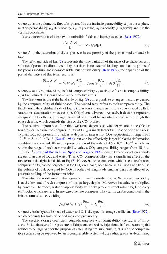
Consider injection of supercritical CO2 in a deep confined saline aquifer (see a schematicdescription in Fig. 2). Momentum conservation is expressed using Darcy’s law, which forphases CO2, c, and brine, w, is given by

qα = −kkrα

μα

(∇ Pα + ραg∇z) , α = c, w, (1)

Fig. 2 Problem setup. Injection of compressible CO2 in a homogeneous horizontal deep saline aquifer

123

CO2 Compressibility Effects

where qα is the volumetric flux of α-phase, k is the intrinsic permeability, krα is the α-phaserelative permeability, μα its viscosity, Pα its pressure, ρα its density, g is gravity and z is thevertical coordinate.

Mass conservation of these two immiscible fluids can be expressed as (Bear 1972),

∂(ρα Sαφ)

∂t= −∇ · (ραqα) , (2)

where Sα is the saturation of the α-phase, φ is the porosity of the porous medium and t istime.

The left-hand side of Eq. (2) represents the time variation of the mass of α-phase per unitvolume of porous medium. Assuming that there is no external loading, and that the grains ofthe porous medium are incompressible, but not stationary (Bear 1972), the expansion of thepartial derivative of this term results in

∂(ρα Sαφ)

∂t= Sαφραcα

∂ Pα

∂t+ ρα Sαcr

∂ Pα

∂t+ ραφ

∂Sα

∂t. (3)

where cα = (1/ρα)(dρα/dPα) is fluid compressibility, cr = dεv/dσ ′ is rock compressibility,εv is the volumetric strain and σ ′ is the effective stress.

The first term in the right-hand side of Eq. (3) corresponds to changes in storage causedby the compressibility of fluid phases. The second term refers to rock compressibility. Thethird term in the right-hand side of Eq. (3) represents changes in the mass of α caused by fluidsaturation–desaturation processes (i.e. CO2 plume advance). As such, it does not representcompressibility effects, although its actual value will be sensitive to pressure through thephase density, which controls the size of the CO2 plume.

The relative importance of the first two terms depends on whether we are in the CO2 orbrine zones, because the compressibility of CO2 is much larger than that of brine and rock.Typical rock compressibility values at depths of interest for CO2 sequestration range from10−11 to 5 × 10−9 Pa−1 (Neuzil 1986), but can be effectively larger if plastic deformationconditions are reached. Water compressibility is of the order of 4.5×10−10 Pa−1, which lieswithin the range of rock compressibility values. CO2 compressibility ranges from 10−9 to10−8 Pa−1 (Law and Bachu 1996; Span and Wagner 1996), one to two orders of magnitudegreater than that of rock and water. Thus, CO2 compressibility has a significant effect on thefirst term in the right-hand side of Eq. (3). However, the second term, which accounts for rockcompressibility, can be neglected in the CO2-rich zone, both because it is small and becausethe volume of rock occupied by CO2 is orders of magnitude smaller than that affected bypressure buildup of the formation brine.

The situation is different in the region occupied by resident water. Water compressibilityis at the low end of rock compressibilities at large depths. Moreover, its value is multipliedby porosity. Therefore, water compressibility will only play a relevant role in high porositystiff rocks, which are rare. In any case, the two compressibility terms can be combined in thebrine saturated zone, yielding

ρwg (φcw + cr)∂hw

∂t= Ss

∂hw

∂t, (4)

where hw is the hydraulic head of water, and Ss is the specific storage coefficient (Bear 1972),which accounts for both brine and rock compressibility.

The specific storage coefficient controls, together with permeability, the radius of influ-ence, R (i.e. the size of the pressure buildup cone caused by injection). In fact, assuming theaquifer to be large and for the purpose of calculating pressure buildup, this infinite compress-ible system can be replaced by an incompressible system whose radius grows as determined

123

V. Vilarrasa et al.

from the comparison between Thiem’s solution (steady state) (Thiem 1906) and Jacob’ssolution (transient) (Cooper and Jacob 1946)

�Pw = Q0μw

4πkdln

(R2

r2

)= Q0μw

4πkdln

(2.25kρwgt

μwr2Ss

), (5)

where Q0 is the volumetric flow rate, μw is the viscosity of water, k is the intrinsic permeabil-ity of the aquifer, d is the aquifer thickness and r is radial distance. The radius of influencecan then be defined from Eq. (5) as

R =√

2.25kρwgt

μwSs. (6)

CO2 is lighter than brine and density differences affect flow via buoyancy. To quantify therelative influence of buoyancy we define a gravity number, N , as the ratio of gravity to viscousforces. The latter can be represented by the horizontal pressure gradient (Q0μ/(2πkrd)),and the former by the buoyancy force (�ρg) in Darcy’s law, expressed in terms of equiv-alent head. This would yield the traditional gravity number for incompressible flow (e.g.Lake 1989). However, for compressible fluids, the boundary condition is usually expressedin terms of the mass flow rate, Qm (Fig. 2). Therefore, it is more appropriate to write Q0 asQm/ρ. Hence, N becomes

N = k�ρgρ̄c2πrcd

μc Qm, (7)

where �ρ is the difference between the fluids density, ρ̄c is a characteristic density, rc is acharacteristic length and Qm is the CO2 mass flow rate. Large gravity numbers (N >> 1)indicate that gravity forces dominate. Small gravity numbers (N << 1) indicate that viscousforces dominate. Gravity numbers close to one indicate that gravity and viscous forces arecomparable.

The characteristic density can be chosen as the mean CO2 density of the plume. Thecharacteristic length depends on the scale of interest (Kopp et al. 2009). The gravity numberincreases with the characteristic length, thus increasing the relative importance of gravityforces with respect to viscous forces (Tchelepi and Orr Jr. 1994). This implies that, as theCO2 plume becomes large, gravity forces will dominate far from the injection well.

These equations can be solved numerically, e.g. (Aziz and Settari 2002; Chen et al. 2006;Pruess et al. 2004). However, creating a numerical model for each potential candidate sitemay require a significant cost. Alternatively, the problem can be solved analytically usingsome simplifications. The use of analytical solutions is useful because (i) they are instanta-neous (Stauffer et al. 2009), (ii) numerical solutions can be coupled with analytical solutionsto make them more efficient (Celia and Nordbotten 2009) and (iii) they identify importantscaling relationships that give insight into the balance of the physical driving mechanisms.

3 Analytical Solutions

3.1 Abrupt Interface Approximation

The abrupt interface approximation considers that the two fluids, CO2 and brine in this case,are immiscible and separated by a sharp interface. The saturation of each fluid is assumed

123

CO2 Compressibility Effects

constant in each fluid region and capillary effects are usually neglected. Neglecting com-pressibility and considering a quasi-steady (successive steady-states) description of movingfronts in Eq. (2) yields that the volumetric flux defined in (1) is divergence free. In addition,if the Dupuit assumption is adopted in a horizontal radial aquifer and Sα is set to 1, i.e. theα-phase relative permeability equals 1, the following equation can be derived (Bear 1972)

1

r

∂

∂r

[ζ

Q0 − 2πr�ρg(k/μc) (d − ζ ) ∂ζ/∂r

ζ + (d − ζ ) μw/μc

]+ 2πφ

∂ζ

∂t= 0, (8)

where ζ is the distance from the base of the aquifer to the interface position and Q0 isthe volumetric flow rate. To account for a residual saturation of the formation brine, Srw ,behind the CO2 front, one should replace μc by μc/k

′rc

in Eq. (8) and below, where k′rc

is theCO2 relative permeability evaluated at the residual brine saturation Srw . Equation (8) can beexpressed in dimensionless form using

rD = r

rc, ζD = ζ

d, tD = t

tc, M = krw/μw

krc/μc, N , (9)

where M is the mobility ratio, N is the gravity number defined in Eq. (7), tc is the characteristictime and the subscript D denotes a dimensionless variable, which yields

1

rD

∂

∂rD

[ζD

1 − rD N (d/rc) (1 − ζD) ∂ζD/∂rD

ζD + (1 − ζD) /M

]+ ∂ζD

∂tD= 0. (10)

Equation (10) shows that the problem depends on two parameters, N and M . The mobilityratio will have values around 0.1 for CO2 sequestration, which will lead to the formation of athin layer of CO2 along the top of the aquifer (Hesse et al. 2007, 2008; Juanes et al. 2009). Onthe other hand, the gravity number can vary over several orders of magnitude, depending onthe aquifer permeability and the injection rate. Thus, the gravity number is the key parametergoverning the interface position.

The analytical solutions of Nordbotten et al. (2005) and Dentz and Tartakovsky (2009a)to determine the interface position of the CO2 plume when injecting supercritical CO2 in adeep saline aquifer start from this approximation.

3.2 Nordbotten et al. (2005) Approach

To find the interface position, Nordbotten et al. (2005) solve Eq. (8) neglecting the gravityterm and approximating the transient system response to injection into an infinite aquiferby a solution to the steady-state problem with a moving outer boundary whose locationincreases in proportion to

√t in a radial geometry, i.e. the radius of influence defined in

(6). In addition, they impose (i) volume balance, (ii) gravity override (CO2 plume travelspreferentially along the top) and (iii) they minimize energy at the well. The fluid pressureapplies over the entire thickness of the aquifer and fluid properties are vertically averaged.The vertically averaged properties are defined as a linear weighting between the propertiesof the two phases. Nordbotten et al. (2005) write their solution as a function of the mobility,λα , defined as the ratio of relative permeability to viscosity, λα = krα /μα . For the case of anabrupt interface where both sides of the interface are fully saturated with the correspondingphase, the relative permeability is 1 and λ becomes the inverse of the viscosity of each phase.These viscosities are assumed constant.

123

V. Vilarrasa et al.

Under these assumptions, Nordbotten et al. (2005) obtain the interface position as,

ζN (r, t) = d

[1 − μc

μw − μc

(√μwV (t)

μcφπdr2 − 1

)], (11)

where V (t) = Q0 · t is the CO2 volume assuming a constant CO2 density.Integrating the flow equation and assuming vertically integrated properties of the fluid

over the entire thickness of the formation, Nordbotten et al. (2005) provide the followingexpression for fluid pressure buildup

PN(r, t) − P0 = Q0μw

2πk

R∫r

dr

r[(

μw−μcμc

)(d − ζ(r)) + d

] , (12)

where PN is the vertically averaged pressure, P0 is the vertically averaged initial pressureprior to injection, Q0 is the volumetric CO2 injection flow rate, k is the intrinsic permeabilityof the aquifer, r is the radial distance and R is the radius of influence.

3.3 Dentz and Tartakovsky (2009a) Approach

Dentz and Tartakovsky (2009a) also consider an abrupt interface approximation. Theyinclude buoyancy effects, and the densities and viscosities of each phase are assumed con-stant.

They combine Darcy’s law with the Dupuit assumption in radial coordinates. Imposingfluid pressure continuity at the interface they obtain

ζDT (r, t) = dγcw ln

[r

rb(t)

], (13)

where rb is the radius of the interface at the base of the aquifer, and γcw is a dimensionlessparameter that measures the relative importance of viscous and gravity forces

γcw = Q0

2πkd2g

�μ

�ρ, (14)

where �μ = μw − μc is the difference between fluid viscosities and �ρ = ρw − ρc is thedifference between fluid densities.

The interface radius at the base of the aquifer is obtained from volume balance as

rb (t) =√

2Q0t

πφdγcw

[exp

(2

γcw

)− 1

]−1

. (15)

Note that the fluid viscosity contrast is treated differently in the two approaches (i.e. mobil-ity ratio and viscosity difference). The mobility ratio is particularly relevant in multiphaseflow when the two phases coexist. However, when one phase displaces the other, the viscositydifference governs the process (see Eq. (14) in Dentz and Tartakovsky (2009a) solution). Anexception to this is the case when fluid properties are integrated vertically (Nordbotten et al.2005), which can be thought of as a coexistence of phases.

123

CO2 Compressibility Effects

4 Compressibility Correction

Let us assume that we have an initial estimation of the mean CO2 density and viscosity.With this we can calculate the interface position using either analytical solutions (11) or (13).Furthermore, the fluid pressure can be calculated from Darcy’s law. Then, the density canbe determined within the plume assuming that it is solely a function of pressure. Integratingthe CO2 density within the plume and dividing it by the volume of the plume, we obtain themean CO2 density

ρc = 1

V

d∫0

r(ζ )∫0

2πφrρc(Pc)drdz, (16)

where V is the volume occupied by the CO2 plume and r(ζ ) is the distance from the well tothe interface position from either Nordbotten et al. (2005) or Dentz and Tartakovsky (2009a).

Note here that we do not specify a priori a particular relationship between density andpressure. We only specify that density is solely a function of pressure. CO2 density alsodepends on temperature (Garcia 2003). However, we neglect thermal effects within the aqui-fer, and take the mean temperature of the aquifer as representative of the system. This assump-tion is commonly used in CO2 injection simulations (e.g. Law and Bachu (1996); Pruess andGarcia (2002)) and may be considered valid if CO2 does not expand rapidly. If this happens,CO2 will experience strong cooling due to the Joule–Thomson effect.

The relationship between pressure and density in Eq. (16) is in general non-linear. More-over, pressure varies in space. Notice that the dependence is two-way: CO2 density dependsexplicitly on fluid pressure, but fluid pressure also depends on density, because density con-trols the plume volume, and thus the fluid pressure through the volume of water that needs tobe displaced. Therefore, an iterative scheme is needed to solve this non-linear problem. Asdensity varies moderately with pressure, a Picard algorithm should converge, provided thatthe initial approximation is not too far from the solution.

The formulation of this iterative approach requires an expression for the spatial variabilityof fluid pressure for each of the two analytical solutions. In the approach of Nordbotten et al.(2005), we obtain an expression for the vertically averaged pressure by introducing (11) into(12) and integrating. The expression for pressure depends on the region: close to the injectionwell, all fluid is CO2; far away, all fluid is saline water; in between the two phases coexistwith an abrupt interface between them,

r > r0; PN (r, t) = P0 + Q0μw

2πkdln

(R

r

),

rb ≤ r ≤ r0; PN (r, t) = P0 + Q0μw

2πkd

[ln

(R

r0

)+

√μcφπd

μwV (t)(r0 − r)

],

r < rb; PN (r, t) = P0 + Q0μw

2πkd

[ln

(R

r0

)+

√μcφπd

μwV (t)(r0 − rb) + μc

μwln

(rb

r

)],

(17)

where r0 is the radial distance where the interface intersects the top of the aquifer, rb is theradial distance where the interface intersects the bottom of the aquifer, P0 = Pt0 + ρwgd/2is the vertically averaged fluid pressure prior to injection, and Pt0 is the initial pressure at thetop of the aquifer. Mathias et al. (2008) come to a similar expression for fluid pressure, but

123

V. Vilarrasa et al.

they consider a slight compressibility in the fluids and rock instead of a radius of influence.The vertically averaged fluid pressure varies with the logarithm of the distance to the well inthe regions where a single phase is present (CO2 or brine). However, it varies linearly in theregion where both phases coexist.

Fluid pressure can be obtained from the Dentz and Tartakovsky (2009a) approach byintegrating (1), assuming hydrostatic pressure (Dupuit approximation) in the aquifer, andtaking the interface position given by (13), which yields

r > r(ζDT); PDT (r, z, t) = Pt0 + ρwg(d − z) + Q0μw

2πkdln

(R

r

),

r ≤ r(ζDT); PDT (r, z, t) = Pt0 + ρwg(d − z) + Q0

2πkd

×(

μw ln

(R

rb

)+ μc ln

(rb

r

)− (μw − μc)

z

dγcw

). (18)

Equation (18) can be averaged over the entire thickness of the aquifer to obtain an aver-aged pressure, which will be used to compare the two approaches. This averaged pressure isgiven by

r > r0; PDT (r, t) = P0 + Q0μw

2πkdln

(R

r

),

rb ≤ r ≤ r0; PDT (r, t) = P0 + Q0

2πkd

[μw

[ln

(R

rb

)+ γcw ln

(r

rb

)ln

(rb

r

)]

+μc ln(rb

r

) [1 − γcw ln

(r

rb

)]

− μw − μc

2γcw

[1 − γ 2

cw

(ln

(r

rb

))2]]

,

r < rb; PDT (r, t) = P0 + Q0

2πkd

[μw ln

(R

rb

)+ μc ln

(rb

r

)− μw − μc

2γcw

]. (19)

Thus, the vertically averaged fluid pressure is defined in three regions in both approaches byEqs. (17) and (19). Unsurprisingly, the two approaches have the same solution in the regionswhere only one phase exists. Differences appear in the region where CO2 and the formationbrine coexist. In the Nordbotten et al. (2005) approach, the vertically averaged pressure varieslinearly with distance to the well. However, in Dentz and Tartakovsky (2009a), it changeslogarithmically with distance to the well. As a result, the approach of Dentz and Tartakovsky(2009a) predicts higher fluid pressure values in this zone.

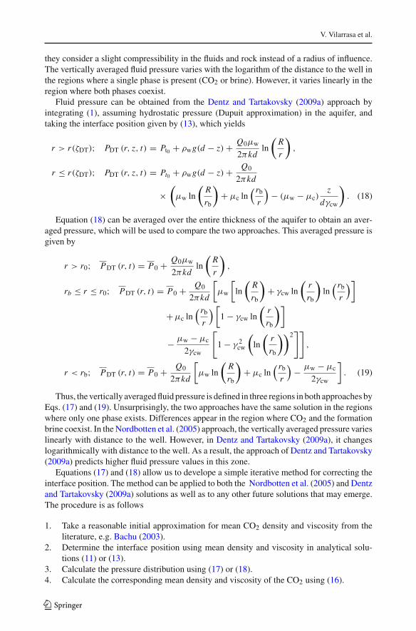
Equations (17) and (18) allow us to develope a simple iterative method for correcting theinterface position. The method can be applied to both the Nordbotten et al. (2005) and Dentzand Tartakovsky (2009a) solutions as well as to any other future solutions that may emerge.The procedure is as follows

1. Take a reasonable initial approximation for mean CO2 density and viscosity from theliterature, e.g. Bachu (2003).

2. Determine the interface position using mean density and viscosity in analytical solu-tions (11) or (13).

3. Calculate the pressure distribution using (17) or (18).4. Calculate the corresponding mean density and viscosity of the CO2 using (16).

123

CO2 Compressibility Effects

5. Repeat steps 2–4 until the solution converges to within some prespecified tolerance.Two different convergence criteria can be chosen: (i) changes in the interface position,or (ii) changes in the mean CO2 density.

The method is relatively easy to implement and can be programmed in a spreadsheet orany code of choice. The method converges rapidly, within a few iterations (typically less than5) in all test cases. A calculation spreadsheet can be downloaded from GHS (2009).

5 Application

5.1 Injection Scenarios

To illustrate the relevance of CO2 compressibility effects, we consider three injection scenar-ios: (i) a regime in which viscous forces dominate gravity forces, (ii) one where both forceshave a similar influence and (iii) a case where gravity forces dominate.

CO2 thermodynamic properties have been widely investigated, e.g. (Sovova and Prochazka1993; Span and Wagner 1996; Garcia 2003). The thermodynamic properties given by Spanand Wagner (1996) are almost identical to the International Union of Pure and AppliedChemistry (IUPAC) (Angus et al. 1976) data sets over the P − T range of CO2 sequestrationinterest (McPherson et al. 2008). However, the algorithm given by Span and Wagner (1996)for evaluating CO2 properties has a very high computational cost. For the sake of simplicityand illustrative purposes, we assume a linear relationship between CO2 density and pressure,given as

ρc = ρ0 + ρ1β(Pc − Pt0), (20)

where ρ0 and ρ1 are constants for the CO2 density, β is the CO2 compressibility, Pc is CO2

pressure and Pt0 is the reference pressure for ρ0. ρ0, ρ1 and β are obtained from data tablesin Span and Wagner (1996). Appendix A contains the expressions for the mean CO2 densityusing this linear approximation in (20) for both approaches.

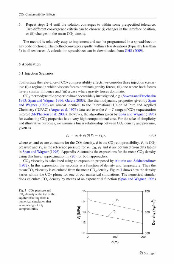
CO2 viscosity is calculated using an expression proposed by Altunin and Sakhabetdinov(1972). In this expression, the viscosity is a function of density and temperature. Thus themean CO2 viscosity is calculated from the mean CO2 density. Figure 3 shows how the densityvaries within the CO2 plume for one of our numerical simulations. The numerical simula-tions calculate CO2 density by means of an exponential function (Span and Wagner 1996)

Fig. 3 CO2 pressure andCO2 density at the top of theaquifer resulting from anumerical simulation thatacknowledges CO2compressibility

11

12

13

14

15

0 500 1000

r (m)

P c (

MP

a)

500

600

700

Den

sity

(kg

/m3)

Pc

c

123

V. Vilarrasa et al.

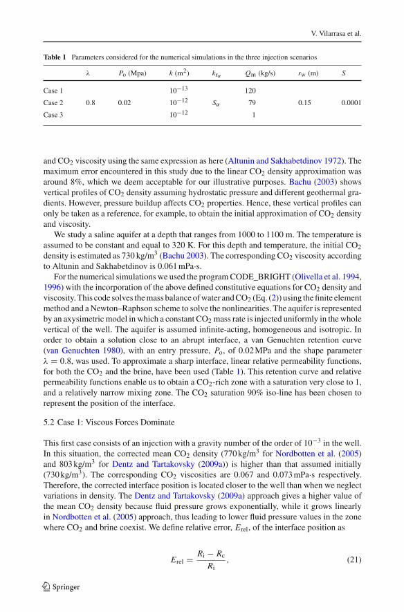
Table 1 Parameters considered for the numerical simulations in the three injection scenarios

λ Po (Mpa) k (m2) krα Qm (kg/s) rw (m) S

Case 1 10−13 120

Case 2 0.8 0.02 10−12 Sα 79 0.15 0.0001

Case 3 10−12 1

and CO2 viscosity using the same expression as here (Altunin and Sakhabetdinov 1972). Themaximum error encountered in this study due to the linear CO2 density approximation wasaround 8%, which we deem acceptable for our illustrative purposes. Bachu (2003) showsvertical profiles of CO2 density assuming hydrostatic pressure and different geothermal gra-dients. However, pressure buildup affects CO2 properties. Hence, these vertical profiles canonly be taken as a reference, for example, to obtain the initial approximation of CO2 densityand viscosity.

We study a saline aquifer at a depth that ranges from 1000 to 1100 m. The temperature isassumed to be constant and equal to 320 K. For this depth and temperature, the initial CO2

density is estimated as 730 kg/m3 (Bachu 2003). The corresponding CO2 viscosity accordingto Altunin and Sakhabetdinov is 0.061 mPa·s.

For the numerical simulations we used the program CODE_BRIGHT (Olivella et al. 1994,1996) with the incorporation of the above defined constitutive equations for CO2 density andviscosity. This code solves the mass balance of water and CO2 (Eq. (2)) using the finite elementmethod and a Newton–Raphson scheme to solve the nonlinearities. The aquifer is representedby an axysimetric model in which a constant CO2 mass rate is injected uniformly in the wholevertical of the well. The aquifer is assumed infinite-acting, homogeneous and isotropic. Inorder to obtain a solution close to an abrupt interface, a van Genuchten retention curve(van Genuchten 1980), with an entry pressure, Po, of 0.02 MPa and the shape parameterλ = 0.8, was used. To approximate a sharp interface, linear relative permeability functions,for both the CO2 and the brine, have been used (Table 1). This retention curve and relativepermeability functions enable us to obtain a CO2-rich zone with a saturation very close to 1,and a relatively narrow mixing zone. The CO2 saturation 90% iso-line has been chosen torepresent the position of the interface.

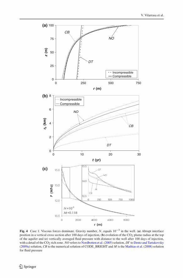
5.2 Case 1: Viscous Forces Dominate

This first case consists of an injection with a gravity number of the order of 10−3 in the well.In this situation, the corrected mean CO2 density (770 kg/m3 for Nordbotten et al. (2005)and 803 kg/m3 for Dentz and Tartakovsky (2009a)) is higher than that assumed initially(730 kg/m3). The corresponding CO2 viscosities are 0.067 and 0.073 mPa·s respectively.Therefore, the corrected interface position is located closer to the well than when we neglectvariations in density. The Dentz and Tartakovsky (2009a) approach gives a higher value ofthe mean CO2 density because fluid pressure grows exponentially, while it grows linearlyin Nordbotten et al. (2005) approach, thus leading to lower fluid pressure values in the zonewhere CO2 and brine coexist. We define relative error, Erel, of the interface position as

Erel = Ri − Rc

Ri, (21)

123

CO2 Compressibility Effects

where Ri is the radius of the CO2 plume at the top of the aquifer for incompressible CO2 andRc is the radius of the CO2 plume at the top of the aquifer for compressible CO2.

Differences between the compressible and incompressible solutions are shown in Fig. 4.For the Dentz and Tartakovsky (2009a) solution, the relative error increases slightly fromthe base to the top of the aquifer, presenting a maximum relative error of 6% at the top ofthe aquifer. For the Nordbotten et al. (2005) solution the interface tilts, with the base of theinterface located just 2% further from the well than its initial position, but the top positioned7% closer to the well. The difference in shape between the two analytical solutions resultsin a CO2 plume that extends further along the top of the aquifer for Nordbotten et al. (2005)solution than Dentz and Tartakovsky (2009a) over time (Fig. 4b). A similar behavior can beseen in the numerical simulations (Fig. 4a). In this case, the interface given by the numericalsimulation compares favourably with that of Nordbotten et al. (2005).

Figure 4c displays a comparison between the vertically averaged fluid pressure given byboth approaches. The fluid pressure given by Mathias et al. (2008) is almost identical tothat obtained in Nordbotten et al. (2005) approach (Eq. (17)). This is because Mathias et al.(2008) assumed the Nordbotten et al. (2005) solution for the interface position and that thehypothesis made therein are valid. The minor difference in fluid pressure between these twoexpressions comes from considering a slight fluid and rock compressibility beyond the plume(recall Section 2). Thus, both expressions can be considered equivalent for the vertically aver-aged fluid pressure. Fluid pressure obtained from the numerical simulation is smaller thanthe other profiles inside the CO2 plume region. This may reflect the larger energy dissipationproduced by analytical solutions as a result of the Dupuit assumption.

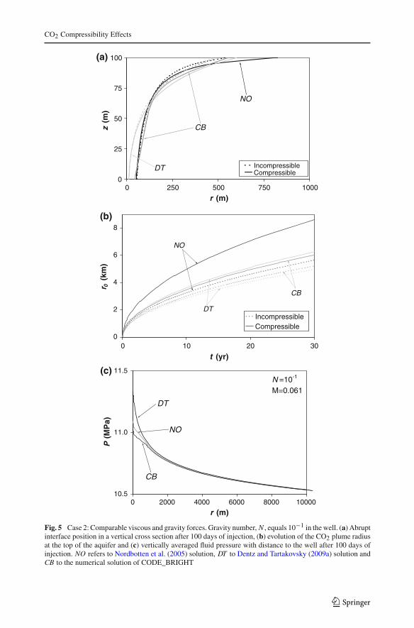
5.3 Case 2: Comparable Gravity and Viscous Forces

Here, the gravity number at the well is in the order of 10−1 (Note that the gravity numberincreases to 1 if we take a characteristic length only 1.5 m away from the injection well.In fact, it keeps increasing further away from the well, where gravity forces will eventuallydominate (recall Section 2)). The density variations between the initial guess of 730kg/m3 andthe corrected value can be large. The density reduces to 512 kg/m3 (viscosity of 0.037 mPa·s)for Nordbotten et al. (2005) and to 493 kg/m3 (viscosity of 0.036 mPa·s) for Dentz andTartakovsky (2009a). This means that the error associated with neglecting CO2 compress-ibility can become very large and should be reflected in the interface position (Fig. 5a). Forthe Dentz and Tartakovsky (2009a) solution including compressibility leads to a 26% error atthe top of the aquifer. This relative error reaches 53% in the Nordbotten et al. (2005) solution.Over a 30 year injection this could represent a potential error of 3 km in the interface positionestimation (Fig. 5b). Here, the numerical simulations also show the importance of consid-ering CO2 compressibility. The interface position from the simulations is similar to that ofNordbotten et al. (2005) in the lower half of the aquifer, where viscous forces may dominate,but it is similar to that of Dentz and Tartakovsky (2009a) in the upper part of the aquifer,where buoyancy begins to dominate.

This dominant buoyancy flow may be significant when considering risks associated withpotential leakage from the aquifer (Nordbotten et al. 2009) or mechanical damage of thecaprock (Vilarrasa et al. 2010), where the extent and pressure distribution of the CO2 on thetop of the aquifer plays a dominant role.

Unlike the previous case, the mean CO2 density of Dentz and Tartakovsky (2009a)approach is lower than that of Nordbotten et al. (2005). This is because Nordbotten et al.(2005) consider the vertically averaged fluid pressure (Fig. 5c). When gravity forces play an

123

V. Vilarrasa et al.

0

25

50

75

100(a)

(b)

(c)

0 250 500 750

r (m)

z (

m)

IncompressibleCompressible

DT

NO

CB

0

2

4

6

8

0 10 20 30

t (yr)

r 0(k

m)

IncompressibleCompressible

DT

NO

CB

Fig. 4 Case 1: Viscous forces dominate. Gravity number, N , equals 10−3 in the well. (a) Abrupt interfaceposition in a vertical cross section after 100 days of injection, (b) evolution of the CO2 plume radius at the topof the aquifer and (c) vertically averaged fluid pressure with distance to the well after 100 days of injection,with a detail of the CO2 rich zone. NO refers to Nordbotten et al. (2005) solution, DT to Dentz and Tartakovsky(2009a) solution, CB to the numerical solution of CODE_BRIGHT and M is the Mathias et al. (2008) solutionfor fluid pressure

123

CO2 Compressibility Effects

0

25

50

75

100

0 250 500 750 1000

r (m)

z (

m)

IncompressibleCompressible

NO

CB

DT

(a)

0

2

4

6

8

0 10 20 30

t (yr)

r 0(k

m)

IncompressibleCompressible

DT

NO

CB

10.5

11.0

11.5

0 2000 4000 6000 8000 10000

r (m)

P (

MP

a)

DT

NO

CB

(c)

(b)

N =10-1

M=0.061

Fig. 5 Case 2: Comparable viscous and gravity forces. Gravity number, N , equals 10−1 in the well. (a) Abruptinterface position in a vertical cross section after 100 days of injection, (b) evolution of the CO2 plume radiusat the top of the aquifer and (c) vertically averaged fluid pressure with distance to the well after 100 days ofinjection. NO refers to Nordbotten et al. (2005) solution, DT to Dentz and Tartakovsky (2009a) solution andCB to the numerical solution of CODE_BRIGHT

123

V. Vilarrasa et al.

important role, the CO2 plume largely extends at the top of the aquifer. CO2 pressure at thetop of the aquifer is lower than the vertically averaged fluid pressure, which considers CO2

and the formation brine. Thus, the mean CO2 density is overestimated when it is calculatedfrom vertically averaged fluid pressure values.

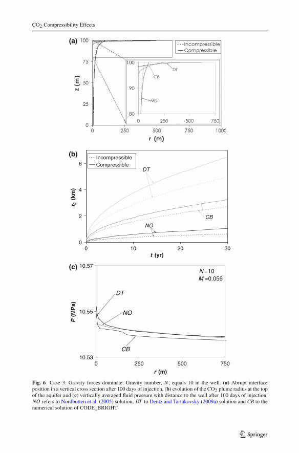
5.4 Case 3: Gravity Forces Dominate

In this case, the gravity number is close to 10 at the well. Density deviations from our ini-tial guess can be very large here. The mean density drops to 479 kg/m3 for Nordbottenet al. (2005) and to 449 kg/m3 for Dentz and Tartakovsky (2009a) solutions, which corre-spond to CO2 viscosities of 0.035 and 0.032 mPa·s respectively. This means that the interfaceposition at the top of the aquifer will extend much further than when not considering CO2

compressibility. The Dentz and Tartakovsky (2009a) solution clearly reflects buoyancy andthe CO2 advances through a very thin layer at the top of the aquifer (Fig. 6a). In contrast,the Nordbotten et al. (2005) interface cannot represent this strong buoyancy effect becausethis solution does not account for gravitational forces. The relative error of the interfaceposition at the top of the aquifer is of 30% for Dentz and Tartakovsky (2009a) solution, andof 64% for Nordbotten et al. (2005). In this case, the numerical simulation compares morefavourably with the Dentz and Tartakovsky (2009a) solution.

The vertically averaged pressure from Dentz and Tartakovsky (2009a) is similar to that ofthe numerical simulation because gravity forces dominate (Fig. 6c). In this case, Nordbottenet al. (2005) predict a very small pressure buildup, which reflects their linear variation withdistance. In addition, the zone with only CO2, where fluid pressure grows logarithmically, isvery limited.

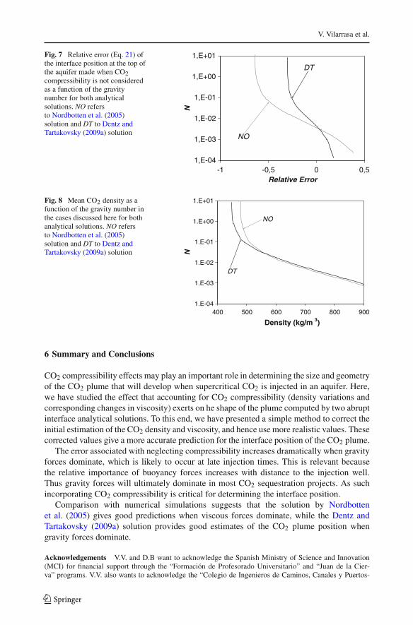
Finally, we consider the influence of the gravity number on CO2 compressibility effects.Figure 7 displays the relative error (Eq. 21) of the interface position at the top of the aqui-fer as a function of the gravity number, computed at the injection well. Negative relativeerrors mean that the interface position extends further when considering CO2 compress-ibility. Both analytical solutions, i.e. Nordbotten et al. (2005) and Dentz and Tartakovsky(2009a), present a similar behaviour, but Nordbotten et al. (2005) has a bigger error. Thisis mainly because they vertically average fluid pressure, which leads to unrealistic CO2

properties in the zone where both CO2 and brine exist. For gravity numbers greater than 1,the mean CO2 density tends to a constant value because fluid pressure buildup in the wellis very small. For this reason, the relative error remains constant for this range of gravitynumbers. However, the absolute relative error decreases until the mean CO2 density equalsthat of the initial approximation for gravity numbers lower than 1. The closer the initialCO2 density approximation is to the actual density, the smaller is the error in the interfaceposition.

Figure 8 displays the mean CO2 density as a function of the gravity number computed inthe well for the cases discussed here. Differences arise between the two analytical approaches.The most relevant difference occurs at high gravity numbers. For gravity numbers greaterthan 5 × 10−2, Nordbotten et al. (2005) yield a higher CO2 density because fluid pressureis averaged over the whole vertical. Thus, fluid pressure in the zone where CO2 and brineexist is overestimated, resulting in higher CO2 density values. For gravity numbers lowerthan 5 × 10−2, CO2 density given by Dentz and Tartakovsky (2009a) is slightly higher thanthat of Nordbotten et al. (2005) because the former predicts higher fluid pressure values inthe CO2-rich zone, as explained previously. However, both approaches present similar meanCO2 density values for low gravity numbers.

123

CO2 Compressibility Effects

0

2

4

6

(a)

(b)

(c)

0 10 20 30t (yr)

r 0(k

m)

IncompressibleCompressible

DT

NO

CB

10.53

10.55

10.57

0 250 500 750

r (m)

P (

MP

a)

DT

NO

CB

N =10M =0.056

Fig. 6 Case 3: Gravity forces dominate. Gravity number, N , equals 10 in the well. (a) Abrupt interfaceposition in a vertical cross section after 100 days of injection, (b) evolution of the CO2 plume radius at the topof the aquifer and (c) vertically averaged fluid pressure with distance to the well after 100 days of injection.NO refers to Nordbotten et al. (2005) solution, DT to Dentz and Tartakovsky (2009a) solution and CB to thenumerical solution of CODE_BRIGHT

123

V. Vilarrasa et al.

Fig. 7 Relative error (Eq. 21) ofthe interface position at the top ofthe aquifer made when CO2compressibility is not consideredas a function of the gravitynumber for both analyticalsolutions. NO refersto Nordbotten et al. (2005)solution and DT to Dentz andTartakovsky (2009a) solution

1,E-04

1,E-03

1,E-02

1,E-01

1,E+00

1,E+01

-1 -0,5 0 0,5Relative Error

N

NO

DT

Fig. 8 Mean CO2 density as afunction of the gravity number inthe cases discussed here for bothanalytical solutions. NO refersto Nordbotten et al. (2005)solution and DT to Dentz andTartakovsky (2009a) solution

1.E-04

1.E-03

1.E-02

1.E-01

1.E+00

1.E+01

400 500 600 700 800 900

Density (kg/m 3)

N

DT

NO

6 Summary and Conclusions

CO2 compressibility effects may play an important role in determining the size and geometryof the CO2 plume that will develop when supercritical CO2 is injected in an aquifer. Here,we have studied the effect that accounting for CO2 compressibility (density variations andcorresponding changes in viscosity) exerts on he shape of the plume computed by two abruptinterface analytical solutions. To this end, we have presented a simple method to correct theinitial estimation of the CO2 density and viscosity, and hence use more realistic values. Thesecorrected values give a more accurate prediction for the interface position of the CO2 plume.

The error associated with neglecting compressibility increases dramatically when gravityforces dominate, which is likely to occur at late injection times. This is relevant becausethe relative importance of buoyancy forces increases with distance to the injection well.Thus gravity forces will ultimately dominate in most CO2 sequestration projects. As suchincorporating CO2 compressibility is critical for determining the interface position.

Comparison with numerical simulations suggests that the solution by Nordbottenet al. (2005) gives good predictions when viscous forces dominate, while the Dentz andTartakovsky (2009a) solution provides good estimates of the CO2 plume position whengravity forces dominate.

Acknowledgements V.V. and D.B want to acknowledge the Spanish Ministry of Science and Innovation(MCI) for financial support through the “Formación de Profesorado Universitario” and “Juan de la Cier-va” programs. V.V. also wants to acknowledge the “Colegio de Ingenieros de Caminos, Canales y Puertos-

123

CO2 Compressibility Effects

Catalunya” for their financial support. Additionally, we would like to acknowledge the ’CIUDEN’ project(Ref.: 030102080014), the ’PSE’ project (Ref.: PSE-120000-2008-6), the ’COLINER’ project and the ’MUS-TANG’ project (from the European Community’s Seventh Framework Programme FP7/2007-2013 under grantagreement no. 227286) for their financial support.

7 Appendix A

Here, the mean CO2 density defined in (16) is calculated using the linear approximation ofCO2 density with respect to pressure presented in (20) for both approaches, i.e. Nordbottenet al. (2005) and Dentz and Tartakovsky (2009a).

With the Nordbotten et al. (2005) approach, the mean CO2 density is calculated by intro-ducing (11) and (17) into (16), which leads to

ρcN= 2πφ

V

{ρ0

d

2r0rb + ρ1β

[r0rb

4ρwgd2 + Q0μw

2πk

[r0rb

(1

2ln

(R

r0

)+ 1

3

)

−r2b

6

(1 − 1

2

μc

μw

)]]}. (22)

Similarly, introducing (13) and (18) into (16), and integrating, yields the expression for themean CO2 density for the Dentz and Tartakovsky (2009a) approach,

ρcDT= 2πφ

V

{(e(2/γcw) − 1

) r2b

4dγcw

[ρ0 + ρ1β

(dγcw

2ρwg

+ Q0

2πkd

(μw ln

(R

rb

)+ μw + μc

2

))]

−r2b

4d2γcwρ1βρwg − e(2/γcw) r2

b

4dρ1β

Q0

2πkdμw

}. (23)

References

Altunin, V.V., Sakhabetdinov, M.A. Viscosity of liquid and gaseous carbon dioxide at temperatures 220-1300 Kand pressure up to 1200 bar. Teploenergetika, 8, 85–89 (1972)

Angus, A., Armstrong, B., Reuck, K.M. (eds.): International thermodynamics tables of the fluid state. Carbondioxide. International Union of Pure and Applied Chemistry. Pergamon Press, Oxford (1976)

Aziz, K., Settari, A. (eds.): Petroleum Reservoir Simulation. 2nd edn. Blitzprint Ltd., Calgary (2002)Bachu, S.: Screening and ranking of sedimentary basins for sequestration of CO2 in geological media in

response to climate change. Environ. Geol. 44, 277–289 (2003)Bachu, S., Adams, J.J.: Sequestration of CO2 in geological media in response to climate change: capacity of

deep saline aquifers to sequester CO2 in solution. Energy Convers. Manag. 44, 3151–3175 (2003)Bear, J. (ed.): Dynamics of Fluids in Porous Media. Elsevier, New York (1972)Bolster, D., Barahona, M., Dentz, M., Fernandez Garcia, D., Sanchez-Vila, X., Trichero, P., Volhondo, C.,

Tartakovsky, D.M. : Probabilistic risk assessment applied to contamination scenarios in porous media.Water Resour. Res. 45, w06413. (2009a) doi:10.1029/2008wR007551

Bolster, D., Dentz, M., Carrera, J.: Effective two phase flow in heterogeneous media under temporal pressurefluctuations. Water Resour. Res. 45, W05408 (2009b). doi:10.1029/2008WR007460

Cantucci, B., Montegrossi, G., Vaselli, O., Tassi, F., Quattrocchi, F., Perkins, E.H.: Geochemical model-ing of CO2 storage in deep reservoirs: the Weyburn Project (Canada) case study. Chem. Geol. 265,181–197 (2009)

Celia, M.A., Nordbotten, J.M.: Practical modeling approaches for geological storage of carbon dioxide. GroundWater 47(5), 627–638 (2009)

123

V. Vilarrasa et al.

Chen, Z., Huan, G., Ma, Y. (eds.): Computational methods for multiphase flows in porous media. SIAM,Philadelphia (2006)

Cooper, H.H., Jacob, C.E.: A generalized graphical method for evaluating formation constants and summa-rizing well field history. Am. Geophys. Union Trans. 27, 526–534 (1946)

Dake, L.P. (ed.): Fundamentals of Reservoir Engineering. Elsevier, Oxford (1978)Dentz, M., Tartakovsky, D.M.: Abrupt-interface solution for carbon dioxide injection into porous media. Trans.

Porous Media 79, 15–27 (2009a)Dentz, M., Tartakovsky, D.M.: Response to “Comments on abrupt-interface solution for carbon dioxide

injection into porous media by Dentz and Tartakovsky (2008)” by Lu et al. Trans. Porous Media 79,39–41 (2009b)

Ennis-King, J., Paterson, L.: The role of convective mixing in the long-term storage of carbon dioxide in deepsaline formations. J. Soc. Pet. Eng. 10(3), 349–356 (2005)

Garcia, J.E.: Fluid Dynamics of Carbon Dioxide Disposal into Saline Aquifers. PhD thesis, University ofCalifornia, Berkeley (2003)

Garcia, J.E., Pruess, K.: Flow Instabilities during injection of CO2 into saline aquifers. Proceedings ToughSymposium 2003, LBNL, Berkeley (2003)

GHS: Spreadsheet with CO2 compressibility correction. http://www.h2ogeo.upc.es/publicaciones/2009/Transport%20in%20porous%20media/Effects%20of%20CO2%20Compressibility%20on%20CO2%20Storage%20in%20Deep%20Saline%20Aquifers.xls (2009)

Hesse, M.A., Tchelepi, H.A., Cantwell, B.J., Orr, F.M. Jr.: Gravity currents in horizontal porous layers: Tran-sition from early to late self-similarity. J. Fluid Mech. 577, 363–383 (2007)

Hesse, M.A., Tchelepi, H.A., Orr, F.M. Jr.: Gravity currents with residual trapping. J. Fluid Mech. 611,35–60 (2008)

Hidalgo, J.J., Carrera, J.: Effect of dispersion on the onset of convection during CO2 sequestration. J. FluidMech. 640, 443–454 (2009)

Hitchon, B., Gunter, W.D., Gentzis, T., Bailey, R.T.: Sedimentary basins and greenhouse gases: a serendipitousassociation. Energy Convers. Manag. 40, 825–843 (1999)

Huppert, H.E., Woods, A.W.: Gravity-driven flows in porous media. J. Fluid Mech. 292, 55–69 (1995)Juanes, R., MacMinn, C.W., Szulczewski, M.L.: The footprint of the CO2 plume during carbon dioxide

storage in saline aquifers: storage efficiency for capillary trapping at the basin scale. Trans. PorousMedia. doi:10.1007/s11242-009-9420-3 (2009)

Katz, D.L., Lee, R.L. (eds.): Natural Gas Engineering. McGraw-Hill, New York (1990)Kopp, A., Class, H., Helmig, R.: Investigation on CO2 storage capacity in saline aquifers Part 1. Dimensional

analysis of flow processes and reservoir characteristics. J. Greenh. Gas Control 3, 263–276 (2009)Korbol, R., Kaddour, A.: Sleipner vest CO2 disposal—injection of removed CO2 into the Utsira

formation. Energy Convers. Manag. 36(6–9), 509–512 (1995)Lake, L.W. (ed.): Enhanced Oil Recovery. Prentice-Hall, Englewood Cliffs, New Jercey (1989)Law, D.H.S., Bachu, S.: Hydrogeological and numerical analysis of CO2 disposal in deep aquifers in the

Alberta sedimentary basin. Energy Convers. Manag. 37(6-8), 1167–1174 (1996)Lu, C., Lee, S.-Y., Han, W.S., McPherson, B.J., Lichtner, P.C.: Comments on “abrupt-interface solution for

carbon dioxide injection into porous media” by M. Dentz and D. Tartakovsky. Trans. Porous Media 79,29–37 (2009)

Lyle, S., Huppert, H.E., Hallworth, M., Bickle, M., Chadwick, A.: Axisymmetric gravity currents in a porousmedium. J Fluid Mech. 543, 293–302 (2005)

Mathias, S.A., Hardisty, P.E., Trudell, M.R., Zimmerman, R.W.: Approximate solutions for pressure buildupduring CO2 injection in brine aquifers. Trans. Porous Media. doi:10.1007/s11242-008-9316-7 (2008)

McPherson, B.J.O.L., Han, W.S., Cole, B.S.: Two equations of state assembled for basic analysis of multiphaseCO2 flow and in deep sedimentary basin conditions. Comput. Geosci. 34, 427–444 (2008)

Neuweiller, I., Attinger, S., Kinzelbach, W., King, P.: Large scale mixing for immiscible displacement inheterogenous porous media. Trans. Porous Media 51, 287–314 (2003)

Neuzil, C.E.: Groundwater flow in low-permeability environments. Water Resour. Res. 22(8),1163–1195 (1986)

Nooner, S.L., Eiken, O., Hermanrud, C., Sasagawa, G.S., Stenvold, T., Zumberge, M.A.: Constraints onthe in situ density of CO2 within the Utsira formation from time-lapse seafloor gravity measurements.J. Greenh. Gas Control 1, 198–214 (2007)

Nordbotten, J.M., Celia, M.A., Bachu, S.: Injection and storage of CO2 in deep saline aquifers: analyticalsolution for CO2 plume evolution during injection. Trans. Porous Media 58, 339–360 (2005)

Nordbotten, J.M., Kavetski, D., Celia, M.A., Bachu, S.: A semi-analytical model estimating leakage associatedwith CO2 storage in large-scale multi-layered geological systems with multiple leaky wells. Environ.Sci. Technol. 43(3), 743–749 (2009). doi:10.1021/es801135v

123

CO2 Compressibility Effects

Olivella, S., Carrera, J., Gens, A., Alonso, E.E.: Non-isothermal multiphase flow of brine and gas throughsaline media. Trans. Porous Media 15, 271–293 (1994)

Olivella, S., Gens, A., Carrera, J., Alonso, E.E.: Numerical formulation for a simulator (CODE_BRIGHT) forthe coupled analysis of saline media. Eng. Comput. 13, 87–112 (1996)

Pruess, K., Garcia, J.: Multiphase flow dynamics during CO2 disposal into saline aquifers. Environ.Geol. 42, 282–295 (2002)

Pruess, K., Garcia, J., Kovscek, T., Oldenburg, C., Rutqvist, J., Steelfel, C., Xu, T.: Code intercomparison buildsconfidence in numerical simulation models for geologic disposal of CO2. Energy 29, 1431–1444 (2004)

Riaz, A., Hesse, M., Tchelepi, H., Orr, F.M. Jr.: Onset of convection in a gravitationally unstable diffusiveboundary layer in porous media. J. Fluid Mech. 548, 87–111 (2006)

Rutqvist, J., Birkholzer, J., Cappa, F., Tsang, C.-F.: Estimating maximum sustainable geological seques-tration of CO2 using coupled fluid flow and geomechanical fault-slip analysis. Energy Convers.Manag. 48, 1798–1807 (2007)

Saripalli, P., McGrail, P.: Semi-analytical approaches to modeling deep well injection of CO2 for geologicalsequestration. Energy Convers. Manag. 43, 185–198 (2002)

Sovova, H., Prochazka, J.: Calculations of compressed carbon dioxide viscosities. Ind. Eng. Chem.Res. 32(12), 3162–3169 (1993)

Span, R., Wagner, W.: A new equation of state for carbon dioxide covering the fluid region from the triple-pointto 1100 K at pressures up to 88 MPa. J. Phys. Chem. Ref. Data 25(6), 1509–1596 (1996)

Stauffer, P.H., Viswanathan, H.S., Pawar, R.J., Guthrie, G.D.: A system model for geologic sequestration ofcarbon dioxide. Environ. Sci. Technol. 43(3), 565–570 (2009)

Tartakovsky, D.M. : Probabilistic risk analysis in subsurface hydrology. Geophys. Res. Lett. 34, L05 404 (2007)Tchelepi, H.A., Orr, F.M. Jr.: Interaction of viscous fingering, permeability inhomogeneity and gravity seg-

regation in three dimensions. SPE Symposium on Reservoir Simulation, New Orleans, pp. 266–271,(1994)

Thiem, G. (ed.): Hydrologische Methode. Leipzig, Gebhardt (1906)Tsang, C.-F., Birkholzer, J., Rutqvist, J.: A comparative review of hydrologic issues involved in geologic

storage of CO2 and injection disposal of liquid waste. Environ. Geol. 54, 1723–1737 (2008)van Genuchten, M.T.: A closed-form equation for predicting the hydraulic conductivity of unsaturated

soils. Soil. Sci. Soc. Am. J. 44, 892–898 (1980)Vilarrasa, V., Bolster, D., Olivella, S., Carrera, J.: Coupled hydromechanical modelling of CO2 sequestration

in deep saline aquifers. Int. J. Greenh. Gas Control (submitted) (2010)Zhou, Q., Birkholzer, J., Tsang, C.-F., Rutqvist, J.: A method for quick assessment of CO2 storage capacity

in closed and semi-closed saline formations. J. Greenh. Gas Control 2, 626–639 (2008)

123