Embed Size (px)
Citation preview

1
GENDER STEREOTYPES IN DELIBERATION AND TEAM DECISIONS1
Katherine Coffman2
Clio Bryant Flikkema3
Olga Shurchkov4
Harvard Business School Wellesley College
First Draft: November 2018
Current Draft: December 2019
Abstract: We explore how groups deliberate and decide on ideas in a laboratory experiment with
free-form communication. We find that gender stereotypes play a significant role in which group
members are rewarded for their ideas when gender is known: conditional on the quality of their
ideas, individuals are less likely to be rewarded by the group in gender incongruent domains (i.e.
male-typed domains for women or female-typed domains for men). This is partly due to
discrimination, and partly due to differences in self-promotion. The conversation data reveal
great similarity across men’s and women’s communication styles, but point to significant biases
in how these styles are perceived.
Key Words: gender differences, stereotypes, leadership, teams, economic experiments
JEL Classifications: C90, J16, J71
1 We thank Manuela Collis, Kyra Frye, and Marema Gaye for excellent research assistance. We also wish to thank
Kristin Butcher, Lucas Coffman, Michael Luca, Corinne Low, Deepak Maholtra, G. Kartini Shastry, and the
participants of the work-in-progress seminar at the University of Massachusetts Amherst and the Wellesley College
Economics Research Seminar for helpful comments. Coffman gratefully acknowledges financial support from
Harvard Business School, and Flikkema and Shurchkov gratefully acknowledge financial support from Wellesley
College Faculty Awards. All remaining errors are our own. 2 Corresponding author. Negotiations, Organizations, & Markets Unit, Harvard Business School, Soldiers Field
Boston, MA, USA, [email protected] 3 Graduated from Wellesley College in 2017, currently in the private sector; [email protected] 4 Corresponding author. Department of Economics, Wellesley College, 106 Central St., Wellesley, MA, USA,

2
I. INTRODUCTION
Across a variety of careers, professional success requires an ability to voice and advocate for ideas
in team decision-making. In this paper, we explore gender differences in the ways in which men
and women communicate in team decision-making problems. We ask whether there are differences
in the propensity of men and women to self-promote themselves and their ideas in these contexts,
and whether they are equally likely to be recognized and rewarded for their ideas.
Although today women make up more than half of the US labor force and earn almost 60%
of advanced degrees, they are not represented proportionally at the highest levels of many
professions (Catalyst 2018). The gender gap in representation as well as earnings is particularly
large in professions dominated by men and perceived to be stereotypically male-oriented, such as
finance (Bertrand et al 2010, Goldin et al 2017) and STEM (Michelmore and Sassler 2016). A
large body of research has investigated how differences in preferences and beliefs contribute to
these gaps (see Niederle 2016 and Shurchkov and Eckel 2018 for surveys).
One strand of work has focused on differences in willingness to contribute ideas in group
settings. Coffman (2014) documents that women are less willing to contribute ideas in
stereotypically male-typed domains, and Bordalo et al (2018) and Chen and Houser (2017) find
that these effects are stronger in mixed-gender groups where gender is known. Similarly, Born et
al (2018) find that women are less willing to be the leader in a group decision-making task,
particularly when the team is majority male. There is also evidence that women are less likely to
receive credit for their contributions. Sarsons (2017) finds that female economists who co-author
with men receive less credit for joint work in terms of tenure probability, and Isaksson (2018) finds
that women claim less credit for team’s successes in a controlled laboratory experiment.
This literature suggests that gender stereotypes may play an important role in
understanding how teams discuss, decide on, and reward ideas. We build on this prior work by
designing a controlled laboratory experiment that utilizes free form chat among group members.
In this way, we take an important step toward studying real world environments of interest, where
“speaking up” and advocating for oneself happens in natural language. In our environment, teams
brainstorm answers to questions that vary according to the gender perception of the topic involved
(the perceived “maleness” of the question). Our first contribution is methodological: the novel
“Family Feud” type task allows for greater subjectivity in the “correctness” of different ideas.
Furthermore, unlike the tasks used in previous studies where there is only one correct answer, our

3
task admits multiple possible answers, some better than others. This creates a setting where ideas
can be contributed, discussed, and debated by teams via free-form chat. Thus, the contribution of
ideas, in our setting, much more closely mirrors real-life decision-making environments as
compared to the more structured experimental paradigms of Coffman (2014), Bordalo et al (2018),
and Chen and Houser (2017).
We are interested both in self-stereotyping, i.e. the ways in which individuals choose to
voice (or not voice) their ideas, and discrimination, i.e. how those ideas and decisions are perceived
by others. Our experimental setting allows us to observe both channels. While the first topic, self-
stereotyping, has been covered in some past work (for instance, by Coffman (2014), the second is
a novel question to be studied within this cleanly controlled setting. To measure discrimination,
we compare behavior across two free form chat treatments that vary whether gender is revealed to
fellow group members. Differences in how contributions are valued and rewarded across these two
treatments would suggest an important role for discrimination. That is, we can ask whether
women’s ideas are more or less valued when they are anonymously contributed.
After groups discuss their ideas via chat, each member provides an incentivized ranking of
everyone in the group, indicating who they would most (and least) like to submit an answer on
behalf of the group. Individuals who are selected to answer on behalf of the group have the
responsibility of aggregating the group discussion into a single group answer that determines each
member’s pay. These selected leaders are also rewarded with additional compensation. Our focus
is on how men and women self-promote (i.e. how they rank themselves) and how they are
evaluated by others.
We find that even though there are no gender differences in individual ability to answer
the Family Feud questions, gender stereotypes play a significant role in which individuals are
rewarded in the known-gender treatment. We observe some self-stereotyping behavior. In the
known-gender treatment, individuals are more likely to self-promote in gender congruent
categories (more female-typed categories for women; more male-typed categories for men). There
is also discrimination when gender is known. Individuals rely on the “maleness” of the question
in determining their rankings, giving more favorable rankings to men (women) as the maleness of
the domain increases (decreases), even conditional on the quality of their contributions. Thus,
significant gender gaps in the individuals that are recognized emerge in the known-gender

4
treatment, both due to self-stereotyping and discrimination. In comparison, there are no gender
gaps in the unknown-gender treatments.
We use control treatments to try to understand the drivers of these gender gaps. In
particular, we ask how much of the gap is driven by the ability of participants to communicate in
natural language. In our control treatments, we remove the opportunity for participants to chat.
Instead, the experimental paradigm restricts participants to “communicate” in a structured, stylized
way. In our most restrictive control treatment, participants simply are forced to volunteer their idea
to the group by submitting an answer that will be viewed by others. This entirely removes the
possibility of self-stereotyping. In a less restrictive control treatment, participants both submit an
answer and indicate how confident they are in that answer. This allows us to ask whether
differences in self-expressed confidence are a driving force in the gender gaps we observe. For
instance, with forced contribution but endogenous voicing of confidence, will women’s ideas be
selected less often, even absent communication? Interestingly, when we restrict communication in
these control treatments, gender gaps are eliminated even when gender is known. Thus, an
important contribution of our work is to show that natural language communication seems to
exacerbate gender gaps and reliance on gender stereotypes, and to begin to unpack why.
We analyze the conversation data to provide further insights into the team decision-making
process. This novel component of our analysis allows us to ask exactly how men and women
advocate for and decide on ideas in these team environments, and identify where (if anywhere)
key gender differences emerge. Third-party external evaluators read chat transcripts and provide
their assessments of each group member across a variety of dimensions. They do so blinded to the
gender of the participants. Interestingly, and perhaps contrary to widely-held beliefs, we find no
significant gender differences in the way in which men and women communicate. That is, when
blind to gender, our external evaluators rate men and women highly similarly across each
dimension, including assertiveness and warmth. Despite this, we find a powerful role for gender
stereotypes in the raters’ perceptions: evaluators of conversations believe that a warm participant
is significantly more likely to be female, and that a negative or critical participant is significantly
more likely to be male. Male raters also believe that members who they judged as competent are
significantly less likely to be female.
Our final step is to use the external analysis of the chat data to predict outcomes in the
group decision-making task. That is, we can ask what features of a participant (i.e., her

5
assertiveness, her warmth, etc., as rated by the coders) make her more or less likely to be chosen
as a group representative by the other members of her group, and whether this varies by gender.
In particular, is assertiveness or warmth a good predictor of being a good team leader, and if so,
do groups recognize this and rank those members highly? Do they do so to a similar degree for
men and women, or do gender stereotypes distort these decisions? For instance, men may be more
likely than women to be recognized by the group for assertiveness -- a trait that is stereotypically
and normatively associated with men.
We explore the returns to warmth, competency/assertiveness, and negativity in our group
decision-making task. Assertiveness and warmth are both associated with being a good team leader
(i.e., an individual who is well-able to identify and submit a high-scoring answer for the group).
But, while groups are quite successful at rewarding assertiveness in their choosing of group leaders
(both among men and women), they are much less successful at rewarding warmth. Even though
warmth is a strong predictor of being a good group representative, warmer participants are less
likely to be promoted to group representative. This is particularly true for warm women.
Our results are consistent with a growing literature showing the importance of stereotypes
for economic outcomes. For example, Shurchkov (2012), Dreber et al. (2014), and Grosse et al.
(2014) show that gender gaps in willingness to compete become substantially smaller and
insignificant in the context of a more female-typed task as compared to a stereotypically male-
typed task used by Niederle and Vesterlund (2007). Similarly, Hernandez-Arenaz (2018) finds that
men who perceive a task as more male-oriented have more optimistic self-assessments of ability
and are more likely to enter a high-paying tournament. Previous studies have also shown that
female decision-makers are more likely to act in a gender-congruent way when their gender would
be observable to subsequent evaluators (Shurchkov and van Geen 2019). Public observability in
the presence of gender stereotypes has also been shown to significantly decrease women’s
willingness to lead (Alan et al 2017, Born et al 2019), willingness to compete (Buser et al 2017),
and to express ambition (Bursztyn et al. 2017). Our work adds to this literature, highlighting that
the willingness to self-promote also depends upon the observability of gender.
The remainder of the paper is organized as follows. Section II describes the design of the
laboratory experiment. Section III discusses the laboratory data and the results. Section IV
overviews the analysis of conversation data. Section V concludes and suggests directions for
further research.
6
II. THE EXPERIMENT
II.A. THE TASK
Participants in our experiment play multiple rounds of a Family Feud style task.5 Family Feud is
a popular gameshow in which teams attempt to guess how respondents in a survey answered
different questions. To our knowledge our study is the first to use a modified Family Feud game
in an economic experiment. The task was chosen to mirror many of the real-world properties of
group decision problems. In this task, there are many good answers to most questions. Some
answers are better than others, but there is room for disagreement. This feature mimics the real-
world properties of brainstorming that, to our knowledge, has yet to be considered in real-effort
task experiments. The points that are ultimately earned depend upon the answers given by others,
so there is a high degree of subjectivity (but, helpful for our purposes, there is still a clear scoring
system). Individuals could play this game independently, but there is room to learn from and debate
with others.
Our version of Family Feud works as follows. Individuals are shown a question, and the
goal is to guess an answer to the question that would be frequently given by others. Specifically,
the Family Feud questions we source have been previously shown to a 100-person survey panel,
who each gave answers to the question. These panel answers generate the scoring system for the
game. The number of points a given answer is worth is equal to the number of survey respondents
who gave that particular answer. Thus, players in our experiment should aim to provide answers
that were popular among the survey respondents, and hence are worth more points. Consider the
example below which we presented to subjects in the instructions for practice.
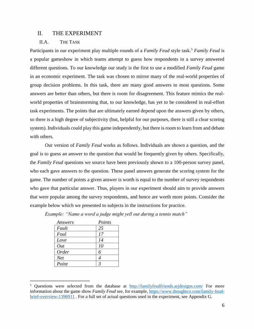
Example: “Name a word a judge might yell out during a tennis match”
5 Questions were selected from the database at http://familyfeudfriends.arjdesigns.com/ For more
information about the game show Family Feud see, for example, https://www.thoughtco.com/family-feud-
brief-overview-1396911 . For a full set of actual questions used in the experiment, see Appendix G.
Answers Points
Fault 25
Foul 17
Love 14
Out 10
Order 6
Net 4
Point 3
7
Here, “fault” receives the most points because 25 out of 100 surveyed individuals stated
this as their answer to the given question. However, “foul” or “love” are still valuable answers, as
they yield some points, albeit less than the top answer. Only answers that receive two or more
survey responses count for points. Note that, for scoring purposes, it does not matter how many
participants in our experiment gave a particular answer; the points were simply based upon these
100-person survey panels constructed by Family Feud. Our participants were informed of this
scoring system, so that they understood that “best” answers were those most popular on the survey
and not necessarily those which they felt were the most correct or the most inventive.6
In summer of 2017, we conducted a pilot on Amazon Mechanical Turk (AMT) to determine
the most appropriate Family Feud questions for the purposes of our study (see details and a
complete set of questions in Appendix G). The goal was to determine common answers to each
question (so that we could program our experiment to accept common variants of each answer),
and to understand the gender stereotype associated with each question. Within the pilot, each AMT
participant provided several answers to a subset of questions drawn from 20 different Family Feud
questions. And, they provided their perception of the gender stereotype for each question,
indicating for each question on a -1 to 1 scale whether they believed men or women would be
better at answering that particular question. Using this data, we selected 8 questions: four
perceived as female-typed and four perceived as male-typed. We use these 8 questions in our main
experiment, randomly assigning one to each round of the experiment at the session level. The
extent to which a question is perceived to carry a male-typed stereotype, as perceived by these
AMT pilot participants, informs one of our main variables in the subsequent analysis. We refer to
this as the “maleness” index, which ranges from -0.57 (the average slider scale rating of the most
female-typed question) to 0.51 (the average slider scale rating of the most male-typed question).
We are interested in how behavior responds to the extent to which a given question is gender
congruent: more male-typed for men, or more female-typed for women. Thus, we will predict
outcomes from the “gender stereotype” of a question: for men, this is exactly the maleness index
of the question, and for women, it is the maleness index re-signed (-1*maleness). This allows us
6 Subjects were also cautioned to check the spelling of their submissions, since misspelled answers could
similarly result in a score of zero points. In practice, we coded the experimental program to accept common
misspellings and common variants of each possible answer. These were sourced through an online pilot.
But, we still wanted to caution participants that we could not guarantee that misspellings would be
recognized.

8
to ask, for any individual, how behavior changes as the question becomes more or less gender
congruent. The set of questions we used is provided in Appendix G.
II.B. EXPERIMENTAL DESIGN
In our experiment, participants play repeated rounds of the Family Feud game, each time in a new
group with stranger matching. Each session of the experiment consisted of two parts, each
containing four rounds of interactions, using one of eight Family Feud questions. In each round,
participants were randomly re-matched in groups of three, using stranger matching. All interaction
took place via private computer terminals.
Our primary treatment variation is whether or not gender information is made available to
participants. In the unknown-gender treatment (UG), participants were identified in each round by
a randomly-generated ID number. In the known-gender treatment (KG), we revealed gender to
participants. We did this in two ways. First, we had group members provide their first name at the
beginning of the treatment. They were encouraged to use their real name, but participants were
able to select any name they wished.7 This name was then used throughout the part to identify
them to their fellow group members during their computer interactions. Second, we did a verbal
roll call, in which groups were announced out loud, and each member of the group was called by
their provided name and asked to respond “here”. In this way, the rest of their group members
were likely to identify their gender, even if their name was ambiguous (as in Bordalo et al 2018).
Note that because the laboratory was equipped with partitions and participants remained seated at
their private terminals, participants were unlikely to view their fellow group members during this
process. Thus, while they learn their group member’s name and hear their voice, they do not see
what they look like.8
In addition to the gender reveal treatments, we varied the extent to which group members could
communicate with one another. In addition to our main chat treatments, where subjects freely
communicated via computerized chat, we have two control treatments aimed at understanding the
7 91% of participants report in the post-experiment questionnaire that they used their real name. We use
this indicator as a control variable in our specifications. 8 One might ask whether participants were likely to know other individuals in their session. We ask
participants in the post-survey questionnaire whether they recognized anyone in their sessions; 85% of
participants report they did not recognize anyone in their session. We then asked, if they did recognize
someone, whether that knowledge changed any of their decisions: 92% of participants report that it did not.

9
mechanisms at work. The control treatments parallel the chat treatments, but eliminate the
opportunity to chat. In the answer only control treatment, we simply display the answers submitted
in the pre-group stage during the group stage. In the answer plus confidence treatment, we display
both the answers submitted and the self-confidence rating from the pre-group stage during the
group stage (more detail on these treatments is provided after our main analysis, in Section III.B).
In each session, subjects participated in exactly two treatments, one in each part. In every case,
one of these treatments was a Known Gender (KG) treatment and the other was an Unknown
Gender (UG) treatment, and at most one was a chat treatment. Figure 1 summarizes the way in
which subjects were randomized into treatments.
Figure 1: Randomization into Experimental Treatments (KG = Known Gender; UG = Unknown
Gender)
Figure 2 summarizes the stages and the flow of the experiment. Each round began with a
“pre-group” stage where participants had 15 seconds to view the question and 30 seconds to submit
an individual answer. After submitting the answer, subjects were asked: “On a scale of 1-10, please
indicate how confident you feel about your ability to submit a high-scoring answer to this specific
question.” This gives us a pre-group measure of individual ability and individual confidence.
Next, subjects entered the “group” stage where they could chat over the computer interface
for 60 seconds with each other. This gave groups a chance to volunteer, debate, and discuss
KG
CHAT
KG
CONTROLUG
CHAT
UG
CONTROL
PART ONE
• Four rounds of play
• Stranger re-matching each
round within part
• Unique Family Feud question
each round
KG
CHAT
KG
CONTROL
UG
CONTROL
UG
CONTROL
UG
CHATKG
CONTROL
PART TWO
• Four rounds of play
• Stranger re-matching each
round within part
• Unique Family Feud question
each round
START

10
different answers. At the end of the chat, participants view a chat transcript. Chat entries are
identified either by names (known-gender) or by ID number (unknown-gender).
Participants then ranked each member of their group, including themselves, from 1 – 3,
where 1 indicated the person they would most want to answer on behalf of the group, i.e. be “the
group representative.” Within each group, we randomly chose one participant whose ranking
would then determine the actual group representative (random dictatorship). We used that
randomly-selected participant’s ranking to probabilistically select a group representative: the
person they ranked first had a 60% chance of being the group representative; the person they
ranked second had a 30% chance; the person they ranked third had a 10% chance. In this way, we
incentivize each group member to provide a complete ranking of the entire group, as any
participant could be chosen to determine the group representative, and their full ranking is relevant
for this determination. Alongside this ranking, each group member also provided a subjective
“confidence” of each group member’s ability to provide a high scoring answer to that question
(again on a 1 – 10 scale).
The “group representative” is important, both because he or she determines which answer
will be submitted on behalf of the group, aggregating the group’s discussion into a single,
collective outcome, and also because he or she will receive a material incentive for being selected
to serve in this capacity – a bonus of $2. In this way, being chosen as the group representative
carries responsibility and increased compensation, reflecting realistic incentives to being
recognized for one’s contributions and to being promoted to positions of leadership.
Finally, there was a “post-group” stage where subjects again submitted individual answers
to the same Family Feud question. Subjects knew that, if they were selected as the “group
representative,” this would be the answer submitted on their behalf. This also allows us to
document how individual answers were influenced by the group discussion, and to provide the
counterfactual of how each individual would have performed if they had been chosen as the group
representative.

11
Figure 2: Stages of the Experiment
II.C. INCENTIVES AND LOGISTICS
One round was randomly selected for payment at the end of the experiment. Participants were paid
based upon one of three submissions in that round: there was a 10% chance they were paid for
their individual answer in pre-group stage, an 80% chance they were paid for the group answer
given by the selected representative, and a 10% chance they were paid for their individual answer
in the post-group stage. In addition, the person selected as the “group representative” received a
bonus payment of $2, providing a material incentive to be chosen.
One pilot session (data excluded from analysis) and 19 sessions of the experiment were
conducted at the Computer Lab for Experimental Research (CLER) at Harvard Business School
(HBS) between September 2017—May 2018. In total, we have 297 participants, each of whom
participated in two treatments. In our primary analysis, we focus on our main chat treatments: 207
subjects participated in our main chat treatments, 105 in the Known Gender version and 102 in the
Unknown Gender version.
GROUP ASSIGNMENT
• Roll call with voices performed in KG
PRE-GROUP STAGE
• Provide initial answer to Family Feud
question
• Provide initial self-confidence
CHAT GROUP STAGE
• Chat with group members
for 60 seconds
• Other members identified by
name in KG
POST-GROUP STAGE
• Provide (updated) answer to Family
Feud question
• Rank group members from 1 – 3
• Provide confidence in each group
member
ANSWER ONLY GROUP
STAGE
• View other group members’
initial answers
• Other members identified by
name in KG
ANSWER AND CONF. GROUP
STAGE
• View other group members’ initial
answers and self-confidence
• Other members identified by name
in KG
OR OR

12
Notes: Each subject was assigned to a known gender treatment in one part of the experiment, and an unknown
gender treatment in the other part of the experiment. The total number of unique subjects is 297.
After signing the informed consent form, participants were seated at individual computer
terminals. Subjects received written, oral, and on-screen instructions programmed using the
standard zTree software package (Fischbacher 2007). Participants were encouraged to ask
questions in private if they did not understand these instructions, but communication between
subjects was disallowed other than when instructed. Subjects only received the instructions
relevant to the immediate part of the experiment (Part 1 or 2). At the end of the experiment, subjects
were informed about their performance and payment and filled out a post-experiment
questionnaire with demographic questions (instructions and questionnaire are available in the
online Appendices H1 and H2). Each session of the experiment lasted approximately one hour.
Subjects were paid in cash and in private by the experimenters. Mean payment across all sessions,
including the show-up fee, was equal to $26.48.
III. RESULTS
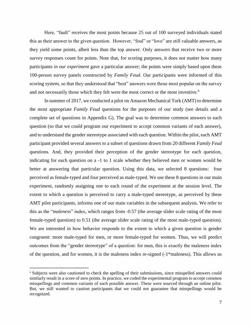
Table 1 below provides summary statistics. On average, we find no statistically significant
differences in any of the demographic characteristics by gender, other than that our male subjects
are significantly more likely to identify as Hispanic (12%) than our female subjects (4.7%).
Men and women do not significantly differ in average performance: in the pre-group stage,
men earn 14.1 points and women earn 13.1 points (t-test p-value of 0.37). However, men earn
$2.21 more than women in the chat treatments (t-test p-value of 0.09). We confirm balance on
demographics across the chat and the control treatments (and recall that all subjects participate in
our known gender and unknown gender treatments). In order to improve precision of our estimates,
we control for individual characteristics in our main analysis.
Known Gender Unknown Gender Total Subjects
Main condition: chat via computer 105 102 207
Control: answer + confidence observable 87 87 174
Control: only answer observable 105 108 213
Total subjects 297 297 594
13
Table 1: Comparison of Demographic Characteristics and Experimental Variables
by Gender in the Chat Treatment
Notes: GPA averages are based on 95 responding males and 103 responding females. Columns 4 and 5 report p-
values. Two-sample tests of proportions for dummy variables produce similar results. Significance levels: *10 percent,
**5 percent, ***1 percent.
Male Female
Absolute
Difference t-test
Mann-Whitney
U test
Demographics
Age (Years) 24.58 24.42 0.16 0.859 0.968
Never Married (%) 85.0% 89.7% 0.05 0.308 0.307
White (%) 36.0% 36.4% 0.00 0.947 0.947
Black (%) 14.0% 18.7% 0.05 0.365 0.364
Asian (%) 39.0% 40.2% 0.01 0.862 0.862
Hispanic (%) 12.0% 4.7% 0.073* 0.055 0.056
Native English (%) 79.0% 77.6% 0.01 0.804 0.804
Born in US (%) 57.0% 57.9% 0.01 0.891 0.891
US Citizen (%) 64.0% 65.4% 0.01 0.832 0.831
Income > $65,000 (%) 52.0% 46.7% 0.05 0.451 0.450
Currently a Student (%) 99.0% 97.2% 0.02 0.349 0.347
Undergraduate (%) 52.0% 45.8% 0.06 0.375 0.373
Primary Field of Study:
Arts & Humanities 12.0% 12.1% 0.00 0.974 0.974
Social Sciences & Business 37.0% 29.0% 0.08 0.221 0.220
Natural Sciences & Engineering 33.0% 41.1% 0.08 0.229 0.228
Other Major 18.0% 17.8% 0.00 0.964 0.964
Used Real Name (%) 93.0% 88.8% 0.04 0.296 0.295
GPA (Points) 3.51 3.47 0.04 0.440 0.736
Final Payment ($) 27.81 25.60 2.212* 0.087 0.092
Number of obs. 100 107
Experimental Variables
Points in Pre-Group Stage 14.06 13.14 0.92 0.368 0.486
Confidence in Pre-Group Stage 7.73 7.59 0.14 0.351 0.080
Total Probability Chosen 32.98 33.66 0.68 0.425 0.359
Points in Post-Group Stage 18.04 17.99 0.05 0.960 0.913
Number of obs. 400 428

14
III. A. PROBABILITY OF BEING CHOSEN AS GROUP REPRESENTATIVE
We start by considering our main outcome of interest: what is the probability that a given
individual is chosen as the group representative? Recall that following the group chat, each
member of the group is asked to provide a ranking of the three group members, self-included. The
first ranked member is assigned a 60% chance of being chosen as group representative, the second
ranked member is assigned a 30% chance of being chosen as a group representative, and the last
ranked member is assigned a 10% chance of being chosen as a group representative. To construct
the probability that a given member is chosen as a group representative, we look at the rankings
provided by her two other group members, and her own, and compute her probability of being
chosen given these rankings. In the tables below, this variable is presented on a 0 – 100 scale.
In Table 2, Columns 1 and 2, we use a linear probability model to predict the probability
that a given member is chosen as group representative, splitting the analysis by treatment (KG and
UG).9 We are interested in the likelihood of being chosen conditional on an individual’s baseline
ability – i.e. her ability to provide a high-scoring answer prior to the group stage. That is, given
two similarly talented individuals ex ante, do differences emerge in how likely they are to be
chosen after the group stage? We proxy for baseline ability by controlling for the quality of
individual pre-group answer (points her pre-group answer would earn), the quality of her
individual pre-group answer relative to the mean quality of individual pre-group answers in her
group (i.e. the difference between points that would be earned by her given answer less average
points for individual pre-group answers in her group), and the quality of the individual answer
relative to the best pre-group answer in her group (i.e. the difference between points that would be
earned by her given answer less points for highest-scoring individual pre-group answer in her
group). We also control for part and round fixed effects, as well as demographic characteristics,
and we cluster standard errors at the group level.
9 Ordered probit specifications deliver similar results.

15
Table 2: The Determinants of the Probability of Being Chosen as the Group
Representative in the Post-Group Stage
Notes: Coefficients obtained using a linear probability model. Sample is restricted to chat
treatment data only. Dependent variable mean is 33.33. All specifications include fixed
effects for round and part; demographic controls for age, student status, race, English
language proficiency, income, use of real name, dummy for whether the US is the country of
citizenship and birth; and controls for performance distribution that include difference from
maximum group score and difference from average group score. Note that in the Chat
treatment, unlike the other two treatments, the pre-group answers of other group members
were not displayed to participants. Robust standard errors clustered at the group level in
parentheses. Significance levels: *10 percent, **5 percent, ***1 percent.
Our main question is whether gender stereotypes predict probability of being chosen,
conditional on baseline ability. To get at this, we regress the probability of being chosen on a
measure of the gender congruence of the question. For men in the sample, this is the “maleness”
variable; for women, we reverse the sign on maleness. This variable, which we call the Gender
Stereotype of the Question, tells us whether gender stereotypes – the extent to which the question
is gender congruent for a given individual – predict the likelihood of being selected. As the
question becomes more male-typed (female-typed), are men (women) more likely to be chosen?
We also test for whether there are gender differences, unconditional on the gender stereotype of
the question, by including a dummy for being female. If women are simply less likely to be chosen
overall, independent of the gender-type of the domain, we predict a significant, negative
coefficient on female, and a coefficient of zero on the gender stereotype term. If, on the other hand,
gender stereotypes, not simply gender, are the driving force, we expect a positive coefficient on
the gender stereotype of the question.
Sample KG UG KG UG
(1) (2) (3) (4)
Female -0.0115 1.779 -0.00530 1.715
(1.362) (1.312) (1.371) (1.291)
Gender Stereotype of Question 3.578** -1.095 3.673** -1.072
(1.787) (2.001) (1.799) (1.999)
Own Gender Share in Group 2.698 1.069
(1.700) (1.637)
Points in Pre-Group Stage 0.00366 -0.00561 0.0103 -0.00240
(0.0553) (0.0687) (0.0555) (0.0696)
R-squared 0.111 0.128 0.116 0.129
Observations (clusters) 420 (105) 408 (102) 420 (105) 408 (102)

16
Columns 1 and 2 present our results, showing that when gender is known, gender
stereotypes do predict the likelihood of being chosen as the group representative. Column 1 shows
that in the known gender treatment, the gender stereotype of the question predicts the probability
of being chosen. We estimate that moving from one end of the “maleness” scale (the most extreme
male-typed value of 1) to the other (the most extreme female-typed value of -1), would increase
the chances that a given female was selected by approximately 7pp, while decreasing the chances
that a given male was selected by the same 7pp. There is no evidence for a similar pattern in the
unknown gender treatment (Column 2). In Columns 3 and 4, we ask whether this result depends
upon the gender composition of the group. We ask for a given individual, how her probability of
being chosen changes as the share of her own gender among the other two group members varies
(for example, for a woman this varies from 0/2 women to 2/2 women). This allows us to gauge
whether being in the majority (a woman among other women, or a man among other men) impacts
decisions. Overall, we estimate that being in the majority seems to directionally increase the
chances of being chosen, but the effect is not significant in either treatment.
With these results in mind, we now turn to understanding what underlies these findings.
Our first step is to decompose the probability of being chosen into two parts: how an individual
rank’s herself, and how others rank that individual. Separating these two forces can speak to how
much of the impact of gender stereotypes is operating through self-stereotyping (as demonstrated
through gender differences in self-rankings) versus discrimination (a gender gap in how
individuals are ranked by others).
III. B. MECHANISMS
III. B.1. THE TWO SOURCES OF RANKING
Recall that the probability of being chosen is shaped by two distinct factors: the ranking an
individual receives from others and the participant’s self-ranking (her propensity to self-promote).
Tables 3 and 4 decompose these two channels.

17
Table 3: The Determinants of Probability of Favorable Ranking by Others in the
Post-Group Stage
Notes: Coefficients obtained using a linear probability model. Sample is restricted to chat
treatment data only. Dependent variable mean is 26.67 in KG and 25.36 in UG. All
specifications include fixed effects for round and part; demographic controls for age, student
status, race, English language proficiency, income, use of real name, dummy for whether the
US is the country of citizenship and birth, and ranker gender; and controls for performance
distribution that include difference from maximum group score and difference from average
group score. Note that in the Chat treatment, unlike the other two treatments, the pre-group
answers of other group members were not displayed to participants. Robust standard errors
clustered at the group level in parentheses. Significance levels: *10 percent, **5 percent, ***1
percent.
First, we consider the ranking by others in Table 3. We parallel the analysis of Table 2,
controlling again for baseline ability, but this time predicting the probability of being chosen only
according to the rankings of the two other group members. Column 1 considers the KG treatment
and shows that the gender stereotyping observed in Table 2 is driven, at least in part, by rankings
by others. As the question becomes more gender congruent, individuals are more likely to be
chosen by others. Notably, this is only true in the KG treatment. When we turn our attention to the
UG treatment in Column 2, we see no role for gender stereotypes in predicting rankings by others.
This suggests that discrimination is a prime channel: when group members know gender, they rank
others more in line with gender stereotypes (conditional on the quality of answers provided). In
Columns 3 and 4, we include the variable for female share among other group members. Female
share has no significant impact on ranking by others.
We now turn our attention to self-rankings. We start by simply noting that the modal action
for participants is to rank themselves first – with participants giving themselves the top ranking in
Sample KG UG KG UG
(1) (2) (3) (4)
Female 0.730 2.099 0.731 2.065
(1.395) (1.385) (1.396) (1.386)
Gender Stereotype of Question 4.489** -0.470 4.521** -0.458
(2.068) (2.113) (2.072) (2.114)
Own Gender Share in Group 0.874 0.567
(1.762) (1.460)
Points in Pre-Group Stage -0.123*** -0.0450 -0.121*** -0.0433
(0.0443) (0.0623) (0.0446) (0.0624)
R-squared 0.068 0.068 0.068 0.069
Observations (clusters) 840 (140) 816 (136) 840 (140) 816 (136)

18
68% of interactions. They rank themselves second in another 19% of interactions, and last in only
12% of interactions. This behavior could be driven by overconfidence – with participants believing
they have a greater chance of submitting a high-scoring answer than the other group members, or
by financial incentives – with participants responding to the bonus payment associated with being
the chosen representative.
Table 4: The Determinants of Probability of Favorable Ranking by Self in the Post-
Group Stage
Notes: Coefficients obtained using a linear probability model. Sample is restricted to chat
treatment data only. Dependent variable mean is 46.67 in KG and 49.26 in UG. All
specifications include fixed effects for round and part; demographic controls for age, student
status, race, English language proficiency, income, use of real name, dummy for whether
the US is the country of citizenship and birth; and controls for performance distribution that
include difference from maximum group score and difference from average group score.
Robust standard errors clustered at the group level in parentheses. Significance levels: *10
percent, **5 percent, ***1 percent.
The analysis in Table 4 parallels Table 2, but this time predicting the probability of being
chosen only according to self-ranking, again on a 0 – 100 scale. Columns 1 and 2 suggest that
overall, men and women self-promote to a similar extent, both in the KG and UG treatments. And,
contrary to what we see saw in the rankings by others, gender stereotypes do not seem to be a
central factor. Thus, the reliance on stereotypes documented in Table 2 for the KG treatment seems
mostly due to the differences in how individuals are ranked by others, not in how they rank
themselves. This is an interesting finding, and at odds with previous work in this area (for instance,
Coffman (2014), Chen and Houser (2017), or Bordalo et al (2019). One important explanation
Sample KG UG KG UG
(1) (2) (3) (4)
Female -1.469 1.150 -1.455 1.026
(2.104) (2.211) (2.113) (2.188)
Gender Stereotype of Question 1.677 -2.355 1.896 -2.308
(2.592) (2.778) (2.572) (2.765)
Own Gender Share in Group 6.276** 2.090
(2.613) (2.655)
Points in Pre-Group Stage 0.256*** 0.0715 0.272*** 0.0778
(0.0966) (0.121) (0.0960) (0.121)
R-squared 0.105 0.099 0.118 0.101
Observations (clusters) 420 (105) 408 (102) 420 (105) 408 (102)

19
could be the role for incentives. In each of these previous papers, group member incentives were
entirely aligned: there were no bonus payments associated with being the person who submitted
the answer for the group. In our framework, there is a clear and non-trivial financial reward for
being the person chosen to submit. It is possible that this financial incentive is enough to overcome
the impact of self-stereotyping. A second important factor could be the role for deliberation. In our
framework, again contrary to past studies, groups have a chance to hear from each other before
selecting who answers for the group. It might be the case that after having the chance to discuss,
and to take into account other’s answers, there is less of a role for self-stereotyping, in part because
individuals in more gender incongruent domains can incorporate the information and ideas from
others in forming their final answer.
Column 3, however, reveals another interesting pattern. While overall men and women
seem to self-promote to a similar extent in the KG treatment, these decisions are highly sensitive
to group composition. Individuals are less likely to self-promote when they are the minority group
member. That is, as the share of women in the group increases, men are significantly less likely to
rank themselves favorably. Women, on the other hand, self-promote more often as the share of
other women increases. As we might expect (since group composition is only known in the KG
treatment), this is only true when gender is known, as shown by the null effects in Column 4 for
the UG treatment.
These results suggest that both rankings by others and self-ranking contribute to the gender
differences we observe in the probability of being chosen. The reliance on gender stereotypes in
selecting who answers for the group seems to operate primarily through rankings by others, with
individuals being more likely to be selected for gender congruent questions when gender is known.
While self-rankings do not show this same adherence to gender stereotypes, they are sensitive to
the gender composition of the group, with individuals being more likely to self-promote when they
are part of the majority. We summarize our results as follows.
Result 1: When gender is known, individuals are more likely to be chosen as the question becomes
more gender congruent (more male-typed for men; more female-typed for women). This is driven
by rankings by others: gender stereotypes predict how individuals are ranked by others.

20
Result 2: When gender is known, individuals are directionally more likely to be chosen as group
representative when they are among the majority in their group. This is driven by self-rankings:
individuals self-promote significantly less often when they are the minority group member than
when they are in the majority.
In the next section of the paper, we further unpack the drivers of these results. We try to
understand what it is about the known gender environment that produces gender gaps. In particular,
we zoom in on the role of self-confidence, and the expression of self-confidence through free form
chat.
III. B.2. THE IMPORTANCE OF SELF-CONFIDENCE
In this section, we ask whether, despite having similar ability, there are gender differences in self-
confidence about ability, and whether these differences have predictive power for the probability
of being chosen. This could operate through multiple channels. Self-confidence could impact self-
rankings, with less confident individuals giving themselves lower rankings. Alternatively, self-
confidence could impact rankings by others, with less confident individuals expressing their ideas
in a way that compromises their chances of being chosen.
On average, men and women express similar levels of confidence in their ability to provide
a high-scoring answer, with men reporting a confidence of 7.7 on average and women reporting a
confidence of 7.6 (recall this is a 1 – 10 scale, t-test p-value of 0.35 and Mann-Whitney U test p-
value of 0.08). Table 5 explores whether gender stereotypes predict self-confidence, splitting the
analysis by treatment and using a linear regression framework with the same set of controls as our
previous analysis.
In the Known Gender treatment, we estimate that self-confidence is a function of gender
stereotypes, with individuals growing significantly more confident in gender congruent questions.
In this treatment, we do not estimate a gender difference in self-confidence for gender-neutral
questions (as indicated by the zero coefficient on the female dummy). In the Unknown Gender
treatment, we see no predictive power of gender stereotypes. Columns 3 and 4 indicate that self-
confidence is not responsive to the gender composition of the group.

21
Table 5: The Determinants of Confidence in the Pre-Group Stage
Notes: Sample is restricted to chat treatment data only. Dependent variable mean is 7.46 in
KG and 7.85 in UG. All specifications include fixed effects for round and part and
demographic controls for age, student status, race, English language proficiency, income, use
of real name, and dummy for whether the US is the country of citizenship and birth. Robust
standard errors clustered at the individual level in parentheses. Significance levels: *10 percent, **5 percent, ***1 percent.
We next ask whether the inclusion of pre-group confidence as an explanatory variable
partially accounts for our previous findings in Tables 2-4. Table 6 reports the results. On average,
confidence in the pre-group stage significantly impacts the total probability of being chosen in
both treatments (Columns 1 and 2). The effect is driven by self-ranking probability (Columns 5
and 6), rather than by others’ ranking (Columns 3 and 4). Individuals who self-report more
confidence in their ability in the initial stage rate themselves more favorably ex post. This
correlation is arguably unsurprising. However, they are not rated more favorably by others. This
shows that individuals who report more self-confidence ex ante are not more effectively
convincing others of their worthiness of being chosen during the group interaction.
Sample KG UG KG UG
(1) (2) (3) (4)
Female -0.0689 -0.409 -0.0682 -0.434
(0.286) (0.263) (0.287) (0.263)
Gender Stereotype of Question 0.616** -0.147 0.621** -0.136
(0.258) (0.260) (0.259) (0.259)
Own Gender Share in Group 0.138 0.387
(0.304) (0.278)
Points in Pre-Group Stage 0.0188*** 0.0215*** 0.0187*** 0.0214***
(0.00697) (0.00689) (0.00697) (0.00678)
R-squared 0.094 0.152 0.095 0.156
Observations (clusters) 420 (105) 408 (102) 420 (105) 408 (102)

22
Table 6: The Effect of Confidence on the Probability of Favorable Ranking in the Post-Group
Stage
Notes: Coefficients obtained using a linear probability model. Sample is restricted to chat treatment data only.
All specifications include fixed effects for round and part; demographic controls for age, student status, race,
English language proficiency, income, use of real name, dummy for whether the US is the country of
citizenship and birth; and controls for performance distribution that include difference from maximum group
score and difference from average group score. Control for ranker gender is included in Columns 3-4. Robust
standard errors clustered at the group level in parentheses. Significance levels: *10 percent, **5 percent, ***1
percent.
Despite its predictive power for being chosen as the group representative, self-confidence
does not explain the gender differences we observe. Even conditional on self-reported confidence,
we see that gender stereotypes are predictive of how individuals are rated by others in the known
gender treatment. Similarly, self-rankings are sensitive to the gender composition of the group,
even conditional on self-reported confidence.
Result 3: Differences in initial self-confidence do not explain why individuals are more likely to
be selected for more gender congruent questions.
Outcome
Sample KG UG KG UG KG UG
(1) (2) (3) (4) (5) (6)
Female 0.0465 2.021 0.754 2.181 -1.346 1.711
(1.357) (1.302) (1.396) (1.382) (2.093) (2.157)
Gender Stereotype of Question 3.148* -0.887 4.286** -0.387 0.797 -1.893
(1.789) (2.003) (2.087) (2.099) (2.497) (2.743)
Own Gender Share in Group 2.574 0.750 0.819 0.446 6.017** 1.374
(1.669) (1.639) (1.769) (1.478) (2.547) (2.592)
Points in Pre-Group Stage -0.0113 -0.0267 -0.130*** -0.0525 0.226** 0.0234
(0.0574) (0.0702) (0.0465) (0.0655) (0.0920) (0.118)
Confidence in Pre-Group Stage 0.844** 0.748** 0.380 0.283 1.769*** 1.677***
(0.353) (0.287) (0.330) (0.345) (0.605) (0.477)
R-squared 0.135 0.143 0.070 0.069 0.152 0.134
Dep. Var Mean 33.33 33.33 26.67 25.36 46.67 49.26
Observations (clusters) 420 (105) 408 (102) 840 (140) 816 (136) 420 (105) 408 (102)
Total Probability Self-RankingOthers' Ranking

23
III. B.3. THE IMPORTANCE OF FREE-FORM INTERACTION
We have seen that knowing gender seems to be a necessary condition for generating gender
differences. When gender is unknown, gender stereotypes do not factor into self or other rankings.
In this section, we ask whether the opportunity to interact is also a necessary condition for
generating differences. In particular, we ask whether we would see similar patterns of
representative selection if groups were not allowed to chat freely.
We design two control treatments to investigate this question. In each of these treatments,
we eliminate the opportunity to chat, but keep all other aspects of the design the same. In the
Answer Only treatment, we replace the group chat with an opportunity to view each of the other
group member’s pre-group stage individual answers. This allows us to ask whether, just seeing
individuals’ answers, provided with no justifications, expressed confidence, or advocacy, would
be enough to generate gender differences. In the Answer + Confidence treatment, we transmit both
the pre-group stage answers and the self-reported confidence of each group member. This allows
us to ask whether answers, combined with a structured report of self-confidence, is enough to
generate gender differences. In Appendix D, we re-run our main tests on each of these control
groups.
What we find is that neither Answers + Confidence nor Answers Only generates the gender
differences we see in the Chat treatment. If individuals just view each other’s answers, gender
stereotypes do not predict who is chosen as the group representative, even when gender is known.
It is not the case that, after seeing just the individual answers contributed, that women are selected
less often as representatives for male-typed questions. Similarly, even if individuals have a chance
to view answers and self-reported confidence, gender stereotypes are still not predictive of who is
selected as the group representative. This suggests that there are features of the interaction itself
that must drive our results. With this in mind, we turn our attention to better understanding those
interactions.
IV. ANALYSIS OF CONVERSATION DATA
Our experiment produced 276 natural language conversations between groups – a rich dataset that
can yield new insights into the ways in which men and women communicate, advocate, and decide
in groups.

24
IV.A. GENDER DIFFERENCES IN OBJECTIVE CHAT CHARACTERISTICS
We begin with an overview of the trends in our conversation data. In particular, we code five
objective variables: (1) number of engagements, measured as the number of times a participant
enters anything into the chat interface; (2) volume of text, measured as the total number of
characters typed in a given chat by a participant; (3) intensity of engagement, calculated as the
number of characters divided by the number of engagements; (4) share of other members
convinced to submit an individual’s own pre-group stage answer, which takes on the values of 0
(did not convince anyone else), ½ (convinced 1 other group member), or 2/2 (convinced both other
group members); and finally (5) an indicator for whether a given participant switched their answer
in the post-group stage from their original pre-group submission.
Subjects used the 60 second chat period to engage in lively and meaningful discussion. In
no circumstances did we observe instances of abusive language, and in over 90 percent of the
interactions, the chat submission was relevant to answering the question at hand (other than to start
the interaction with a greeting). On average, subjects typed in 6 statements into the chat interface
during a given conversation (i.e., average number of engagements was 6). Only 1 observation had
no engagements, and the maximum number of engagements was 18 (see Appendix E1 for the
distribution). Based on simple t-tests or Mann-Whitney U tests, we find that men and women do
not differ significantly in the number of engagements, volume of text they produce, or the intensity
of a given engagement, either on average or by treatment (see online Appendix E1).
Despite these similarities, in the known gender treatment, men are able to convince more
teammates (41 percent) to adopt their initial answer, while women are only able to convince 34
percent (though the gap is not significant; t-test p-value of 0.145). The directional gap is reversed
in the unknown gender treatment, where women are able to convince 37 percent of others in the
group, while men convince 28 percent (t-test p-value of 0.138). Finally, close to 50 percent of all
subjects change their mind after the group discussion (switched from their initial answer to a new
answer), but there are no significant gender differences in the probability of switching away from
the pre-group stage answer in either treatment.
Table 7 asks how these factors impact the probability of being chosen as the group
representative. We focus on the total probability of being chosen, the aggregation of both self-
ranking and ranking by others, separately for the KG and UG treatments. Analysis split by self and
other is available in Appendix C.

25
Table 7: The Effect of Chat Variables on the Probability of Favorable Ranking in the
Post-Group Stage
Notes: Coefficients obtained using a linear probability model. Sample is restricted
to chat treatment data only. All specifications include fixed effects for round and
part; demographic controls for age, student status, race, English language
proficiency, income, use of real name, dummy for whether the US is the country
of citizenship and birth; and controls for performance distribution that include
difference from maximum group score and difference from average group score.
Robust standard errors clustered at the group level in parentheses. Significance
levels: *10 percent, **5 percent, ***1 percent.
There are three important factors in predicting a favorable ranking in both treatments. First
is the number of times a participant enters a statement into the chat interface (the level of
engagement). More engaged participants are chosen more often as group representatives. Second
is the ability to convince others to adopt one’s initial answer. Note that these regressions condition
on pre-group answer quality, so the fact that convincing others positively predicts being chosen is
not simply picking up on some individuals having better pre-group answers. Third, individuals
who switch from their initial answer to a new answer in the post-group stage are significantly less
likely to be chosen in both treatments.
Table C1 in Appendix C explores the heterogeneity of these effects by gender. We interact
each of these factors of interest with gender to ask whether they are similarly predictive for men
Sample KG UG
(1) (2)
Engagements 0.346* 0.407**
(0.177) (0.199)
Intensity of Engagement 0.0175 0.120**
(0.0657) (0.0605)
Share of Others Convinced 8.412*** 8.094***
(1.710) (1.632)
Switched Answer -7.444*** -5.011***
(1.506) (1.414)
Female 0.828 0.816
(1.180) (1.203)
Points in Pre-Group Stage -0.210*** -0.201***
(0.0517) (0.0732)
R-squared 0.327 0.300
Observations (clusters) 420 (105) 408 (102)
Total Probability of Favorable Ranking

26
and women and whether each of these factors becomes more predictive for more gender congruent
questions. Overall, we see no large differences. It is clear that engagements, the share of others
convinced, and not switching from your original pre-group answer positively predict being chosen
as the group representative. The extent to which these matter does not seem to vary much by gender
or by gender stereotype.
IV.B. METHODOLOGY TO MEASURE SUBJECTIVE CHAT CHARACTERISTICS
Of course, these objective measures can only tell us so much about what happens during the group
chats. We are also interested in exploring more about how these individuals communicate, and
how those communications are perceived by others. To give us more subjective data about these
conversations, we hired external coders to analyze the data. We recruited 1000 Amazon
Mechanical Turk (AMT) workers to read the conversations and provide impressions of the
conversations.10 We are interested in the AMT raters’ perceptions of which of the members made
particularly effective contributions to the group, and in how the different group members may have
varied in their communication style.
Each AMT participant read three randomly-selected transcripts. Importantly, within each
conversation, members were labeled simply as Member 1, 2, or 3. That is, we blind AMT
participants to gender. The design was such that each participant saw no more than one
conversation for each of the eight Family Feud questions used in the study, so as to reduce across-
conversation comparisons. Instructions, which can be found in the online appendix, give detailed
information about how these conversations were randomized and how the conversations were
presented to participants.
For each conversation shown to the participant, she was asked a series of questions about
each member of the conversation, both communication-style focused and performance focused
(see Appendix for instructions). We placed the questions about each member on a separate page,
to reduce confusion and to avoid too many questions on a single page. Each page contained the
10 Workers on AMT have been shown to exhibit similar behavioral patterns and pay attention to the
instructions to the same extent as traditional subjects (Paolacci et al. 2010; Germine et al. 2012). Rand
(2012) reviews replication studies that indicate that AMT data are reliable. We used randomly placed
attention checking questions in order to ensure full attention. The final dataset contains valid responses of
985 AMT raters.

27
full transcript for the participant’s reference. Following the warmth-competence literature (Fiske
et al 2007), we asked participants to evaluate members on three dimensions of warmth (warm,
tolerant, good-natured) and competence (competent, intelligent, confident). We also asked about
how assertive and passive the member was, whether they were supportive or critical of others, and
how stubborn they seemed. These 11 personality traits were presented in one block for each
member, in an order randomized at the individual level.
We also asked AMT participants performance-oriented questions: to what extent each
group member contributed to group success, did a good job voicing their ideas, advocated to be
chosen by the group, impeded the group’s success, advocated for their preferred answer, and had
their ideas listened to by the group. These were again organized into one block and randomized at
the individual level.
The 5-point scale ranged from “not at all” to “extremely” for all questions. At the end of
each conversation question set, the AMT participants had to choose which of the three members
they would vote as the “MVP (most valuable player)” of the group. Finally, after the third (last)
conversation question set, the AMT participants were asked to guess the gender of each of the
three group members who participated in that chat. Note that we only asked this question once
and at the very end of the survey, in order to not give away that our research question concerns
gender differences. The main part of the survey was followed by a brief demographic
questionnaire.
Because these are subjective views, we cannot incentivize participants according to the
truth (i.e. we cannot induce a participant to report honestly about how assertive a participant as
given that there is no objective benchmark). So, to increase concentration and motivate
participants, we provide incentives instead through matching. Following participation, we matched
each participant with another participant who faced one of the same chat transcripts. We then
randomly selected one of the questions about that chat and compared the answers. If both
participants gave the same answer to that question, the participant received an extra $1.50 in bonus
payment, in addition to the $2 participation fee. In this way, we discourage participants from
clicking randomly through the survey.
With 17 scale questions about each member, we have a wealth of data on perceptions of
each individual. In order to categorize questions into broader explanatory factors that are
orthogonal to one another, we performed a principal component decomposition. Importantly, while

28
we of course chose the 17 questions that were asked about each participant in each conversation,
this principal component analysis aggregates this data in a way that is independent of our judgment.
The analysis looks at all of the data collected and organizes it into three orthogonal explanatory
factors. Factor 1 loads heavily on competency, confidence, and assertiveness – aligning closely
with the competence dimension identified by Fiske et al (2007); Factor 2 on warmth, good-
naturedness, being supportive of others, and tolerance – aligning with the warmth dimension
identified by Fiske et al (2007); and Factor 3 on the more negative traits of stubbornness, being
critical of others, and impeding success. In the analysis below, we use these three independently-
identified factors, coded as z-scores (see Appendix E.2 for details).
IVC. GENDER STEREOTYPES IN CHAT DATA
Our main question of interest is whether men and women vary in their communication styles, as
rated by our coders. That is, if we consider our three main dimensions of interest -- competence,
warmth, and negativity – are there gender differences in these dimensions? In Table 8, we show
that men and women are rated as identically competent, warm, and negative based upon their
conversation contributions. That is, when blind to gender, coders perceive men and women as
exactly the same on average on all three dimensions. Note that these results are unchanged if we
consider only the known gender treatment (or unknown gender treatment).
Table 8: Relationship between Gender and the Level of Personality Trait Factor
Notes: Fixed effects include question, round, part, and treatment (gender known or unknown). Robust standard
errors clustered at the subject level in parentheses. Significance levels: *10 percent, **5 percent, ***1 percent.
Depedent Variable Factor 1 ("Competence") Factor 2 ("Warmth") Factor 3 ("Negativity")
(1) (2) (3)
Female 0.00257 0.00417 -0.00803
(0.0554) (0.0426) (0.0338)
Gender Stereotype of Question 0.0553 -0.0504 -0.0428
(0.0583) (0.0499) (0.0428)
Fixed Effects YES YES YES
Observations (clusters) 1,656 (207) 1,656 (207) 1,656 (207)
R-squared 0.028 0.047 0.070

29
We also include the extent to which the question is gender congruent as an explanatory
variable. This allows us to ask whether individuals behave more competently, more warmly, or
more negatively in more gender congruent categories (again, when coders are blind to gender).
Again, we see no significant differences. That is, individuals appear to communicate quite
similarly across more gender congruent questions.
Recall that we ask our coders to guess the gender of the members of the conversations.
Thus, we can ask what predicts the probability that a coder believes that a member is female. Table
9 reports the estimates from an OLS regression that predicts the likelihood that an AMT rater
guessed a given participant was female from their evaluation of that member in terms of the three
conversation factors we identified – Competence, Warmth, and Negativity. Importantly, these
estimates are not causal: we cannot rule out that an unmeasured factor or conversation feature leads
the coder to both evaluate the member in a particular way and guess that he or she is female. These
estimates simply tell us which factors are correlated with a coder believing someone is female.
Table 9: The Effect of Personality Trait Factors on the Prediction that a Participant is Female
Notes: Rater demographics include gender, education, race, and whether the rater attended high school in the US.
Robust standard errors clustered at the rater level in parentheses. Significance levels: *10 percent, **5 percent, ***1
percent.
Column 1 shows that members viewed as warm (coded in Factor 2) by the rater are more
likely to be believed to be female, while members viewed as negative (coded in Factor 3) are more
likely to be believed to be male. Thus, while there are no actual differences in how men and women
SampleAll
Male
Raters
Female
Raters
Male-Typed
Questions
Female-Typed
Questions
(1) (2) (3) (4) (5)
Factor 1 ("Competence") -0.016 -0.047*** 0.017 -0.0306** -0.00578
(0.010) (0.014) (0.013) (0.0143) (0.0131)
Factor 2 ("Warmth") 0.059*** 0.054*** 0.069*** 0.0591*** 0.0616***
(0.009) (0.012) (0.013) (0.0128) (0.0119)
Factor 3 ("Negativity") -0.051*** -0.0433*** -0.063*** -0.0545*** -0.0430***
(0.009) (0.011) (0.014) (0.0130) (0.0122)
Rater Was Female 0.084*** 0.0634** 0.106***
(0.016) (0.0246) (0.0216)
Demographic Controls YES YES YES YES YES
Dependent Var. Mean: 0.425 0.384 0.472 0.390 0.454
Observations (clusters) 2,961 (984) 1,584 (526) 1,377 (459) 1,350 (449) 1,611 (537)
R-squared 0.039 0.039 0.043 0.044 0.042

30
seem to communicate in these settings (at least as perceived by our coders), the coders hold strong
stereotypes about the behavior that is more typical of men or women. Being warm is strongly
associated with being perceived as female; being critical is strongly associated with being
perceived as male. Given the inaccuracy of these stereotypes, it is perhaps not surprising that the
raters are on average quite bad at correctly guessing gender: less than 45% of women are correctly
identified as women.
We can also disaggregate the analysis by rater gender (Columns 2 and 3). Here, we see that
these stereotypes regarding warmth and negativity are exhibited by both male and female raters.
Interestingly, we see that for male raters, viewing a member as competent is associated with a
significantly lower probability that the rater believes that member is female. That is, male raters
(falsely) associate being more competent with being male. This is not true for female raters.
Finally, in Columns 4 and 5, we split the data by the associated gender stereotype of the
question. What we see is that warm participants are similarly likely to be perceived as female in
both male and female-typed domains. More negative participants are similarly likely to be
perceived as male in both male and female-typed domains. However, the extent to which coders
associate competence with being female depends on the gender stereotype. More competent
participants are viewed as less likely to be female, but only in male-typed domains. No such
stereotyping occurs in female-typed domains.
Summing up the evidence on gender stereotypes, we see that raters provide nearly identical
ratings of men and women in our data on competence, warmth, and negativity. Yet, when asked
to guess gender, the same coders incorrectly believe that those individuals that they rated as
warmer or less negative are more likely to be women. Male coders also associate competence less
with being female; competence is also less associated with being female when the domain is male-
typed.
We now turn our attention to how these subjective qualities of conversations inform the
selection of group representatives. The group does best by selecting the individual who will submit
the highest scoring answer in the post-group stage. In our data, we observe the post-group stage
answer from each individual in the group, allowing us to evaluate who would be the best choice
within each group. In this section, we use this valuable data to address two questions: first, which
chat factors predict talent as a group representative? and, second, which chat factors do groups
actually seem to rely on in selecting their group representative?

31
To address the first question, we regress the quality of each individual’s post-group stage
answer – the answer they would submit for the group if chosen as the representative – on the
average factor ratings provided for that person in that conversation by our external coders,
including our standard set of demographic controls and fixed effects. Note that here we omit pre-
group stage ability measures, due to their correlation with the competence dimension.11 Table 10
presents the results.
We observe that directionally, all three factors are positively predictive of submitting a
higher scoring answer. The strongest factor is warmth: warmer participants are significantly better
group representatives (p<0.01). Competence is also a significant predictor (p<0.05); the effect size
is roughly a third smaller.12 Column 2 shows that the extent to which these factors are predictive
of being a good group representative are very similar for men and women. Similarly, Column 3
shows that the extent to which these factors are predictive of being a good group representative do
not vary with how gender congruent the question is. Overall, our results suggest that, if groups
are attempting to maximize group earnings, they should be selecting group representatives who
are competent, and even more importantly warm – independent of gender, or the gender stereotype
of the question.
11 See Appendix Table F1, for specifications that include pre-group stage ability measures. 12 Note that controls for distribution of pre-group performance absorb the positive effects of competence
and warmth on post-group performance. This can likely be explained by the correlation between ability, as
measured by the individual answer in pre-group stage and competence See Appendix Table F1.

32
Table 10: The Effect of Personality Trait Factors on Post-Group Performance
Notes: Sample restricted to chat data treatments only. Demographic controls include
ranker gender and rankee’s age, student status, race, English language proficiency,
income, use of real name, and dummy for whether the US is the country of citizenship
and birth. Fixed effects include round, part, and question, as well as treatment (KG).
Robust standard errors clustered at the rater level in parentheses. Significance levels: *10 percent, **5 percent, ***1 percent.
With this in mind, we return to the rankings provided by the group members and ask how
the three factors of competence, warmth, and negativity predict how members were ranked in the
experiment. That is, consistent with Table 10, do groups do a good job of selecting warm,
competent group representatives? We explore this in Table 11, predicting a participant’s ranking
from her other group members from her average rating on each factor for that conversation. We
Sample
(1) (2) (3)
Factor 1 ("Competence") 1.994** 1.877* 2.083**
(0.838) (1.128) (0.853)
Factor 2 ("Warmth") 3.199*** 3.475** 3.244***
(1.113) (1.727) (1.113)
Factor 3 ("Negativity") 1.457 2.613 1.596
(1.437) (1.953) (1.431)
Female 0.396 0.374 0.346
(0.909) (0.911) (0.949)
Female x Factor 1 0.274
(1.621)
Female x Factor 2 -0.459
(2.209)
Female x Factor 3 -2.331
(2.754)
Gender Stereotype of Question 0.732
(1.461)
Stereotype x Factor 1 1.671
(2.589)
Stereotype x Factor 2 -1.104
(3.079)
Stereotype x Factor 3 1.626
(3.502)
Dependent Var. Mean: 18.01 18.01 18.01
Observations (clusters) 1656 (207) 1656 (207) 1656 (207)
R-squared 0.149 0.150 0.151
All Chat Treatments

33
include the same set of controls as in our main analysis (i.e. the structure of Table 3) to keep the
analysis as parallel as possible. First we note that competence is strongly predictive of receiving a
favorable ranking from others. This is true in both the KG and UG treatments (Columns 1 and 4).
Thus, groups seem to reward competence. However, they do not reward warmth. In fact, warmth
has a negative average impact on ranking in the KG treatment (Column 1), and an insignificant
average effect in the UG treatment (Column 4).
Table 11: The Effect of Chat Behavior Factors on Ranking by Others in Post-Group Stage
Notes: Sample is restricted to chat treatment data only. All specifications include fixed effects for round and part;
demographic controls for age, student status, race, English language proficiency, income, use of real name, dummy
for whether the US is the country of citizenship and birth; ranker gender and controls for performance distribution
that include difference from maximum group score and difference from average group score. Robust standard
errors clustered at the group level in parentheses. Significance levels: *10 percent, **5 percent, ***1 percent.
Sample
(1) (2) (3) (4) (5) (6)
Factor 1 ("Competence") 7.587*** 7.623*** 7.376*** 7.995*** 5.924*** 7.620***
(1.232) (1.556) (1.247) (1.075) (1.468) (1.088)
Factor 2 ("Warmth") -3.527*** -0.879 -3.391*** 0.215 -0.979 0.258
(1.188) (2.132) (1.179) (1.241) (1.786) (1.274)
Factor 3 ("Negativity") -1.945 0.114 -1.954 -2.029 -1.617 -1.969
(1.611) (2.635) (1.628) (1.385) (2.077) (1.367)
Female 0.681 0.867 0.458 2.328* 2.374* 2.435*
(1.346) (1.355) (1.338) (1.244) (1.244) (1.290)
Female x Factor 1 0.301 3.766**
(2.058) (1.786)
Female x Factor 2 -4.740* 1.887
(2.772) (2.379)
Female x Factor 3 -3.422 -0.690
(3.675) (2.981)
Gender Stereotype of Question 2.963 -0.279
(2.051) (2.024)
Stereotype x Factor 1 -1.172 -5.145*
(3.096) (2.867)
Stereotype x Factor 2 0.523 7.536**
(4.111) (3.624)
Stereotype x Factor 3 -2.964 2.031
(5.523) (4.775)
Points in Pre-Group Stage -0.167*** -0.168*** -0.168*** -0.138** -0.136** -0.138**
(0.0489) (0.0496) (0.0516) (0.0637) (0.0637) (0.0635)
R-squared 0.123 0.126 0.128 0.145 0.150 0.154
Observations (clusters) 840 (140) 840 (140) 840 (140) 817 (136) 817 (136) 817 (136)
Probability of Favorable Ranking by Others
KG UG

34
Interestingly, Column 2 reveals that only women in the KG treatment are penalized by
others for warmth. On the other hand, men in the KG treatment (Column 2) and men and women
in the UG treatment (Column 5) receive no such penalty. These results are robust to the inclusion
of controls for distribution of pre-group performance. Furthermore, controlling for our outcome
measure of Table 10 – actual talent as the group representative, i.e. post-group stage individual
performance – does not affect the results in Table 11 and, importantly, has a negligible effect on
the probability of being chosen (both in significance and magnitude, see Appendix Table F2). This
suggests that groups are not particularly capable of selecting good group representatives.
In sum, groups seem to be getting it wrong in a predictable way. The data tell us that
warmth – which loads on being warm, good-natured, tolerant, and supportive of others – is strongly
associated with being a high scoring group representative. While we can only speculate, it may be
that these members are particularly adept at listening to all the answers, and are open to new,
potentially better ideas. But, groups are, if anything, less likely to select warm individuals as
representatives. This is particularly true of warm female members in the known gender treatment.
The competence dimension, which loads on competency, confidence, and assertiveness, on the
other hand, is relied upon very strongly by groups.
Result 4: Groups strongly reward competence, confidence, and assertiveness in selecting group
representatives. Groups do not reward warmth.
V. DISCUSSION
Our paper explores the ways in which gender stereotypes shape group decision-making. In our
novel framework, we allow for free-form chat across group members, providing additional insights
into how gender stereotypes operate. We find that individuals are less likely to be rewarded for
their ideas in gender incongruent domains when gender is known, despite having equal ability and
communicating in a similar style. This is partly due to discrimination by fellow group members,
and partly due to differences in the propensity to self-promote (particularly when they are in the
minority).
The chat data reveal that men and women have very similar styles and contributions to the
group on average, as viewed by our blind-to-gender coders. And yet, our coders demonstrate a
clear bias in their assessment of member gender, incorrectly believing that warm members are

35
more likely to be female, while more negative members are more likely to be men. Male coders
also view more competent members as more likely to be male. Interestingly, while warmth is
strongly associated with being a good group representative, groups do not seem to recognize this:
warm members are less likely to be selected as group representatives. This suggests that
stereotypes about communication styles are pervasive, and may shape the expectations for
behavior in group decision-making contexts.
In many ways, our environment comes closer to “real world” settings than past
experimental work in this space, allowing for free form communication in a subjective decision-
making problem. The fact that we find distortions in contribution and recognition in this
environment raises important questions about how these forces might fuel gender differences in
workplace outcomes. Our work suggests a need for structuring group decision-making in a way
that assures the most talented members both volunteer and are recognized for their contributions,
despite gender stereotypes.

36
REFERENCES
Alan S., Ertac S., Kubilay E., Loranth, G. 2017. “Understanding Gender Differences in
Leadership.” Working paper.
Born, A., Ranehill, E., Sandberg, A. 2018. “A Man’s World? – The Impact of a Male Dominated
Environment on Female Leadership,” University of Gothenburg Working Paper in
Economics No. 744.
Bertrand M, Goldin C, Katz LF. 2010. “Dynamics of the Gender Gap for Young Professionals in
the Financial and Corporate Sectors,” American Economic Journal: Applied Economics, 2
(3): 228-255.
Bordalo, P., Coffman, K. B., Gennaioli N., Schleifer, A. 2018. “Beliefs about Gender,” American
Economic Review, forthcoming.
Bursztyn, L, Fujiwara T, Pallais A. 2017. “‘Acting Wife’: Marriage Market Incentives and Labor
Market Investments,” American Economic Review, 107 (11): 3288-3319.
Catalyst. 2018. “Knowledge Center: Women in S&P 500 Companies,” http://www.catalyst.org.
Chen, J., and Houser, D. 2017. “Gender Composition, Stereotype and the Contribution of Ideas,”
GMU Working Paper in Economics No. 17-26.
Coffman, K. B. 2014. “Evidence on Self-stereotyping and the Contribution of Ideas,” The
Quarterly Journal of Economics, 129(4): 1625–1660.
Dreber, A., von Essen, E., Ranehill, E. 2014. “Gender and Competition in Adolescence: Task
Matters,” Experimental Economics 17 (1): 154–72.
Grosse, N. D., Riener, G., Dertwinkel-Kalt, M. 2014. “Explaining Gender Differences in
Competitiveness: Testing a Theory on Gender-Task Stereotypes,” Mimeo, 1–35.
Germine, L., Nakayama, K., Duchaine, B. C., Chabris, C. F., Chatterjee, G., Wilmer, J. B. 2012.
“Is the Web as Good as the Lab? Comparable Performance from Web and Lab in
Cognitive/Perceptual Experiments,” Psychonomic Bulletin & Review, 19: 847–857.
Goldin, C., Kerr, S. P., Olivetti, C., Barth, E. 2017. “The Expanding Gender Earnings Gap:
Evidence from the LEHD-2000 Census,” American Economic Review: Papers and
Proceedings, 107 (5): 110-114.
Hernandez-Arenaz, I. 2018. “Stereotypes and Tournament Self-Selection: A Theoretical and
Experimental Approach,” University of the Balearic Islands Working Paper.

37
Isaksson, S. 2018. “It Takes Two; Gender Differences in Group Work,” Working paper.
Michelmore, K., Sassler, S. 2016. “Explaining the Gender Wage Gap in STEM: Does Field Sex
Composition Matter?” RSF: The Russell Sage Foundation Journal of the Social Sciences,
2(4): 194–215.
Niederle, M., Vesterlund, L. 2007. “Do Women Shy Away from Competition? Do Men Compete
Too Much?” The Quarterly Journal of Economics 122 (3): 1067–1101.
Niederle, M. 2016. “Gender,” in The Handbook of Experimental Economics 2, Kagel John, Roth
Alvin E., eds. (Princeton, NJ: Princeton University Press, 2016).
Paolacci, G., Chandler, J., Ipeirotis P. G. 2010. “Running Experiments on Amazon Mechanical
Turk,” Judgement and Decision Making, 5: 411–419.
Rand D.G. 2012. “The Promise of Mechanical Turk: How Online Labor Markets Can Help
Theorists Run Behavioral Experiments,” Journal of Theoretical Biology, 299: 172–179.
Sarsons, H. 2017. “Recognition for Group Work: Gender Differences in Academia,” American
Economic Review: Papers and Proceedings, 107 (5): 141-145.
Shurchkov, O. 2012. “Under Pressure: Gender Differences in Output Quality and Quantity under
Competition and Time Constraints,” Journal of the European Economic Association 10
(5): 1189–1213.
Shurchkov, O., Eckel C. C. 2018. “Gender Differences in Behavioral Traits and Labor Market
Outcomes,” in The Oxford Handbook of Women and the Economy, Averett Susan L., Argys
Laura M., Hoffman Saul D., eds. (Oxford, UK: Oxford University Press, 2018).
Shurchkov, O., van Geen, A. 2019. “Why Female Decision‐Makers Shy Away from Promoting
Competition,” Kyklos, 72 (2): 297-331.